The Dapor-Liegener model of Loop Quantum Cosmology: A dynamical analysis

Abstract

The Dapor-Liegener model of Loop Quantum Cosmology (LQC), which depicts an emergent universe from a de Sitter regime in the contracting phase is studied from the mathematical viewpoint of dynamical systems and compared with the standard model of LQC. Dealing with perturbations, on the contrary to standard LQC where at early times all the scales are inside the Hubble radius, we show that it is impossible to implement the matter bounce scenario due to the fact that an emergent de Sitter regime in the contracting phase implies that all the scales are outside of the Hubble radius in a past epoch.

I Introduction

In a recent paper dl (see also dl2 ), applying Thiemann’s procedure for the regularization of the the full Hamiltonian in Loop Quantum Gravity (LQG), Dapor and Liegener have obtained a new effective Hamiltonian for Loop Quantum Cosmology (LQC) which agrees, at the leading order, with the previous one obtained some years ago in ma , but differs from the usual effective Hamiltonian of LQC singh ; singh1 ; singh2 ; singh08 ; singh09 ; as . The difference between both approaches lies in the fact that for an spatially flat and homogeneous universe, the Euclidean and the Lorentz terms of the full Hamiltonian are proportional to each other and in LQC it is usual to write the Lorentz term as the Euclidean one and quantize their combination as . However, this treatment is impossible in the full LQG theory, where the Lorentz term has to be quantized in a different way from of the Euclidean one dl1 , obtaining a completely different effective Hamiltonian.

This new effective Hamiltonian constraint leads, contrarily to standard LQC, to a non-symmetric bouncing background emerging from a de Sitter regime in the contracting phase and ending in the expanding one by matching with General Relativity (GR) dl2 . And, although this model has already been studied in great detail in several papers dl ; singh18 ; agullo , we believe that an analysis from the viewpoint of dynamical systems could simplify the reasoning and help to better understand it.

In fact, working in the plane $(H,\rho)$ where $H$ denotes the Hubble parameter and $\rho$ the energy density of the universe, where the standard model in LQC has the universe crossing and ellipse in clockwise direction, we show that the Dapor-Liegener model has a more complicated behavior presenting two separate asymmetric branches: In the physical one, and always dealing with a non phantom field or fluid filling the universe, the universe emerges from a de Sitter regime evolving, in the contracting phase, to the bounce, where after entering in the expanding phase it evolves asymtotically into a flat expanding universe obeying GR. In the non-physical one one has, at very early times, a flat contracting universe obeying GR and evolving to the bounce, to enter in the expanding phase where it transits to end up in a de Sitter regime. This second branch is not physical, in spite of the low value of the energy density of the universe, due to the high value of the Hubble parameter in this last stage, which is in disagreement with its very low current value.

Once we have studied the dynamics of the model we deal with perturbations, arguing that due to the fact that the universe emerges from a de Sitter regime in the contracting phase, and thus at early times all the scales are outside the Hubble radius, it is impossible for this new approach of LQC to provide either a matter or matter-ekpyrotic bouncing scenario as the ones given by standard LQC, where at the beginning all the scales are inside of the Hubble radius we ; ha14a ; cw ; wilson0 .

The paper is organized as follows: In Section II we review the dynamics of the standard LQC background. Section III is devoted to the analysis of the new approach of LQC obtaining the corresponding modified Friedmann equation and the dynamical equations. Finally, in the last Section we briefly discuss some features of cosmological perturbations in this new scenario using the so-called dressed effective metric approach agullo1 .

The units used throughout the paper are $\hbar=c=1$, and ${8\pi G}=1$.

II Dynamics in standard LQC

We start reviewing the dynamics in standard LQC where the full effective Hamiltonian is given by as ; singh ; singh1 ; singh2 ; singh08 ; singh09

$${\mathcal{H}}_{LQC}={\mathcal{V}}\rho-3{\mathcal{V}}\frac{\sin^{2}(\beta\lambda)}{\gamma^{2}\lambda^{2}},$$ (1)

where $\rho$ is the energy density of the universe, $\gamma\cong 0.2375$ is the Immirzi parameter whose numerical value is obtained comparing the Bekenstein-Hawking formula with the black hole entropy calculated in LQG meissner , although an updated derivation perez shows that the Immirzi parameter is no longer fixed, but only bounded in the LQC setting, by this formula. The parameter $\lambda\equiv\sqrt{\frac{\sqrt{3}}{2}\gamma}$ is the square root of the area gap -the square root of the minimum eigenvalue of the area operator- in LQG (see section II E of as where the authors use an heuristic correspondence between the kinematic states of LQC and those of LQG to conclude that the parameter $\lambda$ is the square root of the minimum eigenvalue of the area operator of LQG), although there are some modified theories leading to the same Friedmann and Raychauduri equations as in standard LQC, where $\lambda$ is a free parameter which has to be determined from observational data. For example, teleparallel LQC saridakis ; haro13 , theories including in the Einstein-Hilbert action a convenient non-linear term of the form $f({\mathcal{R}})$, where ${\mathcal{R}}$ is some scalar such that in the Friedmann-Lemaître-Robertson-Walker (FLRW) spacetime becomes proportional to the Hubble parameter or its square helling ; ds09 ; ha17 or else using a modified version of mimetic gravity hap ; Norbert ; mukhanov1 ; langlois . Finally, ${\mathcal{V}}=a^{3}$ is the volume (to simplify the volume of the cubic fiducial cell has taken to be equal to $1$) and $\beta$ is its conjugate momentum, which classically satisfies $\beta=\gamma H$ acs , being $H$ the Hubble parameter, although and whose Poisson bracket is given by $\{\beta,{\mathcal{V}}\}=\frac{\gamma}{2}$.

The Hamiltonian constraint ${\mathcal{H}}_{LQC}=0$, leads to the following expression of the energy density

$$\rho=3\frac{\sin^{2}(\beta\lambda)}{\gamma^{2}\lambda^{2}},$$ (2)

and the Hamilton equation $\dot{{\mathcal{V}}}=\{{\mathcal{V}},{\mathcal{H}}_{LQC}\}=-\frac{\gamma}{2}\frac{\partial{\mathcal{H}}_{LQC}}{\partial\beta}$ leads to the following expression for the Hubble parameter

$$H=\frac{\sin(2\beta\lambda)}{2\gamma\lambda}.$$ (3)

A simple combination of equations (2) and (3) leads to the holonomy corrected Friedmann equation in standard LQC singh06 ; svv06 ; sst06

$$H^{2}=\frac{\rho}{3}\left(1-\frac{\rho}{\rho_{c}}\right),$$ (4)

where $\rho_{c}=\frac{3}{\gamma^{2}\lambda^{2}}\cong 252$ is the so-called critical energy density in standard LQC singh08 . From this modified Friedmann equation one can see that at low energy densities ($\rho\ll\rho_{c}$) one recovers GR, because this equation becomes the standard Friedmann equation $H^{2}=\frac{\rho}{3}$ which depicts a parabola in the plane $(H,\rho)$. This two curves which at low energy densities coincide, are very different at high energy densities. Effectively, the parabola of GR is unbounded allowing the formation of singularities such as the Big Bang or the Big Rip where the energy density diverges. However, in standard LQC, this kind of singularities are forbidden due to the fact that the ellipse depicted by the Friedmann equation in standard LQC (see FIG. $1$) is a closed bounded curve bho ; aho .

To find the dynamical equation, we have to take into account that holonomy corrections only affect the gravitational sector, for this reason the energy density satisfy the conservation equation $\dot{\rho}=-3H(\rho+P)$, where $P$ is the pressure. Then, taking the derivative of (4) and using the conservation equation one can easily find the Raychauduri equation in standard LQC singh09

$$\dot{H}=-\frac{1}{2}(\rho+P)\left(1-\frac{2\rho}{\rho_{c}}\right).$$ (5)

Note that from the conservation equation one can see that for a fluid or field with effective Equation of State (EoS) parameter $w_{eff}=\frac{P}{\rho}>-1$, that is, for a non-phantom fluid or field, the movement accros the ellipse is clockwise, as has been shown in FIG. $1$.

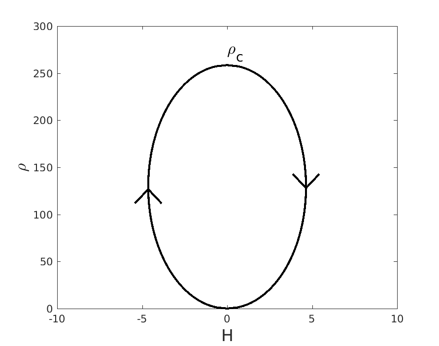
Figure 1: Ellipse depicted by the Friedmann equation in standard LQC, and its dynamics for a non-phantom fluid or field.

Once we have obtained the dynamical equations, we can consider two different cases:

1. A universe filled by a barotropic fluid with EoS $P=P(\rho)$. In this case, the unique background is obtained solving the first order differential equation $\dot{\rho}=-3H_{\pm}(\rho)[\rho+P(\rho)],$ where $H_{+}(\rho)=\sqrt{\frac{\rho}{3}\left(1-\frac{\rho}{\rho_{c}}\right)}$ is the value of the Hubble parameter in the expanding phase and $H_{-}(\rho)=-\sqrt{\frac{\rho}{3}\left(1-\frac{\rho}{\rho_{c}}\right)}$ is its value in the contracting one. In general, this equation has to be solved numerically, but in the particular case of an constant effective EoS parameter $w_{eff}$ one obtains the following analytic solution we :

   $$a=\left(\frac{3}{4}\rho_{c}(1+w_{eff})^{2}t^{2}+1\right)^{\frac{1}{3(1+w_{eff})}},$$

   $$\quad H=\frac{\rho_{c}(1+w_{eff})t}{2a^{3(1+w_{eff})}},\quad\rho=\frac{\rho_{c}}{a^{3(1+w_{eff})}}.$$ (6)

2. A universe filled by an scalar field $\phi$ minimally coupled with gravity. In this case the energy density is $\rho=\frac{\dot{\phi}^{2}}{2}+V(\phi)$, and the conservation equation reads

   $$\ddot{\phi}+3H_{\pm}(\phi,\dot{\phi})\dot{\phi}+V_{\phi}=0,$$ (7)

   where once again $H_{\pm}(\phi,\dot{\phi})=\pm\sqrt{\frac{\rho}{3}\left(1-\frac{\rho}{\rho_{c}}\right)}$.

   The difference with the case of a barotropic fluid is that now we have a second order differential equation, meaning that one has infinitely many backgrounds. Moreover, one could also obtain a potential having a background which is the same as the one provided by a barotropic fluid with constant EoS parameter mielczarek ; haa

   $$V=2\rho_{c}\frac{(1-w_{eff})e^{-\sqrt{3(1+w_{eff})}\phi}}{(1+e^{-\sqrt{3(1+w_{eff})}\phi})^{2}}.$$ (8)

Effectively, inserting this potential in (7) one gets the analytic solution

$${\phi}=\frac{2}{\sqrt{3(1+w_{eff})}}\ln\left(\sqrt{\frac{3}{4}\rho_{c}(1+w_{eff})^{2}}t\right.$$

$$\left.+\sqrt{\frac{3}{4}\rho_{c}(1+w_{eff})^{2}t^{2}+1}\right),$$ (9)

which leads to the background (1). The dynamics provided by the potential (8), i.e., the other non-analytic solutions, was recently studied with great detail in aah ; haa , showing that in the case $|w_{eff}|<1$ all the backgrounds depict a universe with a constant effective EoS parameter equal to $w_{eff}$ at early and late times. On the contrary, when $w_{eff}>1$, the potential (8) becomes ekpyrotic, the backgrounds depict an universe bouncing twice and after the second bounce it enters, in the expanding phase, in a kination regime (its effective EoS parameter is equal to $1$).

III Dynamics in the Dapor-Liegener model of LQC

In the Dapor-Liegener (DL) model the full effective Hamiltonian is given by dl ; ma ; dl2 ; singh18 ; agullo

$${\mathcal{H}}_{DL}={\mathcal{V}}\rho-3{\mathcal{V}}\frac{\sin^{2}(\beta\lambda)}{\gamma^{2}\lambda^{2}}\left(1-(\gamma^{2}+1)\sin^{2}(\beta\lambda)\right),$$ (10)

and the Hamiltonian constraint leads to the following expression of the energy density of the universe

$$\rho=3\frac{\sin^{2}(\beta\lambda)}{\gamma^{2}\lambda^{2}}\left(1-(\gamma^{2}+1)\sin^{2}(\beta\lambda)\right).$$ (11)

In this model, the Hamilton equation $\dot{{\mathcal{V}}}=\{{\mathcal{V}},{\mathcal{H}}_{DL}\}=-\frac{\gamma}{2}\frac{\partial{\mathcal{H}}_{DL}}{\partial\beta}$ leads to the following value of the Hubble parameter

$$H=\frac{\sin(2\beta\lambda)}{2\gamma\lambda}\left(1-2(\gamma^{2}+1)\sin^{2}(\beta\lambda)\right).$$ (12)

Introducing the notation $\sin^{2}(\beta\lambda)\equiv x$, the equation (12) has the form ${\rho}=\rho_{c}f(x)$, where $f$ is a function defined in $[0,1]$ as $f(x)=x-(\gamma^{2}+1)x^{2}$. This function is positive in the interval $[0,\frac{1}{\gamma^{2}+1}]$, and reaches its maximum at $x=\frac{1}{2(\gamma^{2}+1)}$, meaning that the minimum value of the energy density is $0$ and its maximum value is $\rho_{max}=\frac{\rho_{c}}{4(\gamma^{2}+1)}$.

Using this variable $x\in[0,\frac{1}{\gamma^{2}+1}]$ the equation (12) could be written as

$$H^{2}=\frac{x(1-x)\rho_{c}}{3}\left(1-2(\gamma^{2}+1)x\right)^{2},$$ (13)

which in the interval $[0,\frac{1}{\gamma^{2}+1}]$ vanishes when $x=0$, $x=1$ and $x=\frac{1}{2(\gamma^{2}+1)}$ i.e., when $\rho=0$ and $\rho=\rho_{max}$. Note also that, when the energy density vanishes at $x=\frac{1}{\gamma^{2}+1}$, the square of the Hubble parameter does not vanish as in standard LQC. In this theory its value is $\tilde{H}^{2}=\frac{4\gamma^{2}\rho_{max}}{3{\gamma^{2}+1}}$.

After this brief discussion one can conclude that the variable $\beta$ belongs in the interval $[-\beta_{i},\beta_{i}]$ where $\beta_{i}\equiv\frac{1}{\lambda}\arcsin\left(\frac{1}{\sqrt{\gamma^{2}+1}}\right)$. The equations (12) and (11) depict a curve in the plane $(H,\rho)$ whose first branch is obtained when $\beta$ belongs in the interval $[0,\beta_{i}]$ and the second one when the variable belongs in $[-\beta_{i},0]$ (see FIG. $2$).

To find the dynamics we perform the temporal derivative of the energy density (11) obtaining:

$$\dot{\rho}=\frac{6}{\gamma}H\dot{\beta},$$ (14)

and once again taking into account that holonomy corrections only affect the matter sector, the conservation equation will be $\dot{\rho}=-3H(\rho+P)$, and one finally gets the equation

$$\dot{\beta}=-\frac{\gamma}{2}(1+w_{eff})\rho,$$ (15)

where once again $w_{eff}=\frac{P}{\rho}$ denotes the effective EoS parameter.

Since the derivative of $\beta$ is zero when the energy density vanishes, the dynamical system has three fixed points at $\beta=\pm\beta_{i}$ and $\beta=0$, or in the plane $(H,\rho)$, at $(\pm\sqrt{\tilde{H}^{2}},0)$ and $(0,0)$. Therefore, for a non-phantom fluid or field, i.e., when $w_{eff}>-1$, there are two different dynamics:

1. Branch 1 (blue curve in FIG. $2$): The variable $\beta$ moves from $\beta_{i}$ to $0$, or in the plane $(H,\rho)$ the universe emerges in a de Sitter regime moving in the contracting phase from $(-\sqrt{\tilde{H}^{2}},0)$ to $(0,\rho_{max})$, where it bounces to enter in the expanding phase, and finally at late times it ends at $(0,0)$ where GR applies, because when $\beta\cong 0$ the equations (12) and (11) become $H\cong\frac{\beta}{\gamma}$ and $\rho\cong 3\frac{\beta^{2}}{\gamma^{2}}$, thus combining them one gets the standard Friedmann equation $H^{2}\cong\frac{\rho}{3}$, that is, one recovers GR at low energy densities.

2. Branch 2 (red curve in FIG. $2$): The variable $\beta$ moves from $0$ to $-\beta_{i}$, or in the plane $(H,\rho)$ the universe starts when GR is valid, moving in the contracting phase from $(0,0)$ to $(0,\rho_{max})$, where the universe bounces entering in the expanding phase, and finally ending in a de Sitter regime at $(+\sqrt{\tilde{H}^{2}},0)$. Obviously, the dynamics in this second branch is not viable because the universe ends in a de Sitter phase with such a large value of the Hubble parameter.

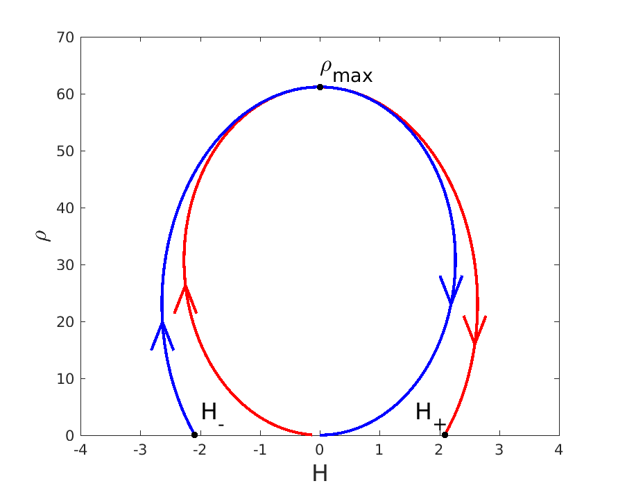
Figure 2: Curve depicted by the Friedmann equation in the Dapor-Liegener model of LQC, and its dynamics for either a non-phantom fluid or field. Blue: branch with $\beta>0$. Red: branch with $\beta<0$.

To obtain explicitly the dynamics one has to solve the equation (15). In the case of a barotropic fluid with EoS $P=P(\rho)$ one has to solve the equation

$$\dot{\beta}=-\frac{\gamma}{2}(\rho+P(\rho)),$$ (16)

with $\rho$ given by equation (11). This is a one dimensional first order differential equation in the variable $\beta$ which, once it is solved, one has to insert in equations (11) and (12) to obtain the dynamics. In the particular case of a constant effective EoS parameter, the equation (16) can be integrated analytically obtaining an implicit equation of the form $F(\sin(\beta\lambda))=t$ but, unfortunately, there is no analytic expression of the inverse of $F$. Therefore, it is impossible to reach a simple expression such as (1) obtained in standard LQC, only numerical calculations can be performed to obtain the dynamics.

When the universe is filled by an scalar field minimally coupled with gravity the problem is more involved because in this case, equation (15) reads

$$\dot{\beta}=-\frac{\gamma}{2}\dot{\phi}^{2},$$ (17)

and it is impossible to express $\dot{\phi}^{2}$ as a function of $\beta$. So, one has to work as in standard LQC, and consider the conservation equation (7), but with another expression of $H_{\pm}(\phi,\dot{\phi})$. To find it, one has to isolate $\sin^{2}(\beta\lambda)$ in (11) and insert it in (12). After some algebra one has

$$H^{2}_{\pm}(\rho)=\frac{\rho}{3(\gamma^{2}+1)}\left(1-\frac{\rho}{\rho_{max}}\right)\times$$

$$\left[1+\frac{2\gamma^{2}}{1\pm\sqrt{1-\frac{\rho}{\rho_{max}}}}\right],$$ (18)

and since at low energy densities $\rho\ll\rho_{max}$ one has $H^{2}_{+}(\rho)\cong\frac{\rho}{3}$ and $H^{2}_{-}(\rho)\cong\tilde{H}^{2}$, the dynamics in the first branch (the physical one) will be given by the equation

$$\ddot{\phi}+3H_{\pm}(\phi,\dot{\phi})\dot{\phi}+V_{\phi}=0,$$ (19)

where we now denote by $H_{+}(\phi,\dot{\phi})$ the value of the Hubble parameter in the expanding phase and $H_{-}(\phi,\dot{\phi})$ in the contracting one, and we have $H_{\pm}(\phi,\dot{\phi})=\pm\sqrt{H^{2}_{\pm}(\rho)}$, with $\rho=\frac{\dot{\phi}^{2}}{2}+V(\phi)$. One can see that equation (19), which as in GR or standard LQC provides infinitely many different backgrounds because it is a second order differential equation, can only be solved numerically.

Another way, the one used in agullo , to find numerically backgrounds is to consider the system

$$\left\{\begin{array}[]{ccc}\dot{\beta}&=&-\frac{\gamma}{2}\psi^{2}\\ \dot{\phi}&=&\psi\\ \dot{\psi}&=&-3H(\beta){\psi}-V_{\phi},\end{array}\right.$$ (23)

where $H(\beta)$ is given by (12). To solve the system one needs three initial conditions, which for simplicity one could take at the bounce, $(\beta_{B},\phi_{B},{\psi}_{B})$. As we have already showed, in the first branch, at the bounce one has $\beta_{B}=\frac{1}{\lambda}\arcsin\left(\frac{1}{\sqrt{2(\gamma^{2}+1)}}\right)$, then one only has to choose a value of $\phi_{B}$ satisfying $V(\phi_{B})\leq\rho_{max}$, because, at the bounce, $\psi_{B}$ is determined by the constraint $\frac{{\psi}_{B}^{2}}{2}+V(\phi_{B})=\rho_{max}$.

Finally, we want to stress that the background provided by the Dapor-Leigener model does not seem easy to be mimicked using modified or mimetic gravity as has been done for the standard model in LQC helling ; Norbert ; langlois , due to the complicated form exhibited by the solution curve to the Friedmann equation (III) in the plane $(H,\rho)$ (see FIG. $2$).

IV Perturbations

There are two different ways to understand a bouncing scenario (see B ; nb08 ; patrick0 ; patrick ; odintsov0 for a review of bouncing cosmologies). One of them is to see it as an implementation of inflation, where the big bang singularity is replaced by a bounce but the inflationary regime exists in the expanding phase bgt ; bgt1 ; barrau ; sloan . The other viewpoint is radically different: a bouncing cosmology, named matter or matter-ekpyrotic bouncing scenario, is an alternative to the inflationary paradigm, and thus, the inflationary phase is removed brandenberger ; brandenberger1 ; brandenberger2 in this scenario.

In the first path, an inflationary potential is used and the observable scales leave the Hubble radius during the inflationary regime as in standard inflation but, unlike in inflation, the modes corresponding to those scales are not expected to be in the so-called adiabatic or, sometimes, Bunch-Davies vacuum (see for instance the section $6.2$ of riotto ), due to their previous evolution in the contracting phase and across the bounce agullo . On the contrary, in the second point of view the modes corresponding to the observable scales, which leave the Hubble radius at very early times in the contracting phase, are in the adiabatic vacuum we ; wilson0 ; cw ; ha14a ; saridakis ; ha17 ; lw , due to the duality between the de Sitter regime in the expanding phase and a matter domination in the contracting phase wands . In fact, to obtain a nearly flat power spectrum in this approach, one has to choose a potential which at early times leads to a quasi-matter domination regime in the contracting era eho .

In standard LQC, both points of view have been implemented with success. The first one has been extensively studied in bgt ; bgt1 ; agullo1 ; agullo2 ; agullo3 , and the second one in we ; wilson0 ; cw ; haa ; eho ; lw ; ha14a ; ha17 studying the matter and the matter-ekpyrotic bounce scenario, and partially showing its viability confronting the theoretical values of spectral quantities such as the spectral index, its running or the ratio of tensor to scalar perturbations with their corresponding observational values.

However, as we will immediately show, in this new version of LQC it is impossible to implement the second viewpoint. Effectively, in LQC there are two ways to deal with perturbations, the deformed algebra approach grain ; vidotto ; lisenfors ; grain1 and the dressed effective metric approach agullo1 ; agullo2 ; agullo3 . Both approaches are performed in the Hamiltonian framework instead of the Lagrangian one, so covariance is not immediately manifest and it is replaced by the invariance under gauge transformations generated by the Hamiltonian constraint $H[N]$ and diffeomorphism constraints $D[N^{a}]$, where $N$ is the smeared lapse function and $N^{a}$ is the smeared shift vector, which satisfy the classical algebra of constraints:

$$\{D[N_{1}^{a}],D[N_{2}^{a}]\}=D[{\mathcal{L}}_{N_{1}}N_{2}^{a}],$$ (24)

$$\{H[N],D[M^{a}]\}=-H[{\mathcal{L}}_{M}N],$$ (25)

$$\{H[N_{1}],H[N_{2}]\}=D[q^{ab}(N_{1}\nabla_{a}N_{2}-N_{2}\nabla_{a}N_{1})].$$ (26)

Then, general covariance in canonical theories is implemented in a more subtle way than in Lagrangian theories. And dealing with the quantization of canonical theories of gravity, two assumption are imposed in order to maintain the covariance (see for instance bojowald0 ; bojowald1 ; bojowald2 ):

1. The algebra of constraints has to be closed

2. The algebra of constraints has to be a well defined classical limit, and in the limit it has to coincide with the classical one: equations (24), (25) and (26).

In the deformed algebra approach applied to standard LQC, the Asthekar connection is replaced by hand by suitable sinusoidal functions grain , and the anomalies, which appear after the replacement, are removed introducing some counter-terms. The obtained algebra of constrains differs from the classical case in the constraint

$$\{H[N_{1}],H[N_{2}]\}=\Omega D[q^{ab}(N_{1}\nabla_{a}N_{2}-N_{2}\nabla_{a}N_{1})],$$ (27)

where $\Omega=1-\frac{2\rho}{\rho_{c}}$. Thus, in the classical limit $\rho_{c}\rightarrow\infty\Longleftrightarrow\gamma\rightarrow 0$, one recovers the classical expression, what means that the deformed algebra approach satisfy both assumptions, and consequently this approach maintains covariance.

On the contrary, in the dressed effective metric approach where the Mukhanov-Sasaki is the same as in GR, but the metric background is replaced by an effective one which differs from the classical one. In fact, the metric background is replaced by the one provided by LQC, what does not seem to preserve the covariance.

On the other hand, there are covariant theories, performed from a Lagrangian formulation, which leads to the same background as standard LQC hap ; hae18 , but the perturbation equations are completely different of those of LQC, this is a point that deserves future investigation because is not clear at all why this equations differs from the ones of the deformed algebra approach which, as we have already seen, is also covariant.

Dealing with the Dapor-Liegener model of LQC, due to the difficult form of the corresponding Friedmann equation (eq. (III)), so far the perturbation equations are not obtained either in the deformed algebra approach or in any covariant Lagrangian formulation. For this reason, although it not seems covariant, to deal with the perturbed equations in the DP model of LQC, at the present time, one has to use the dressed effective metric approach. However, as we will immediately see, the chosen perturbative approach will not affect our claim about the impossibility to implement the matter bounce scenario in the DP model of LQC, because in this scenario the observable modes must leave the Hubble radius at very low energy density where holonomy corrections become negligible, and thus, during this period, the perturbative equations become the same as in GR.

Thus, studying scalar perturbations in this last approach, the Mukhanov-Sasaki (M-S) equation will be in conformal time agullo3

$$v_{k}^{\prime\prime}+\left(k^{2}+\mathfrak{U}-\frac{a^{\prime\prime}}{a}\right)v_{k}=0,$$ (28)

where the potential $\mathfrak{U}$ is given by

$$\mathfrak{U}=\left(V\frac{3\dot{\phi}^{2}}{\rho}-2V_{\phi}\sqrt{\frac{3\dot{\phi}^{2}}{\rho}}+V_{\phi\phi}\right)a^{2}.$$ (29)

Dealing, for instance, with a quartic chaotic potential $V=\lambda\phi^{4}$, at very early times, i.e., when $\rho\cong 0$, and thus with $\phi\cong 0$ and $\dot{\phi}\cong 0$, one will have $\mathfrak{U}\cong 12\lambda\phi^{2}a^{2}$.

Remark IV.1

The backgrounds provided by power law potentials $V=\lambda\phi^{2n}$, which has been reproduced numerically for the particular case of a quadratic potencial (see for instance singh18 ), are not difficult to understand in LQC. At very early times, since the energy density is zero, the field is at the bottom of the potential starting to oscillate to gaing energy because it is in the contracting phase (recall the conservation equation $\dot{\rho}=-3H\dot{\phi}^{2}$). In fact, in the Dapor-Liegener model, contrary to standard LQC, due to the high value of the Hubble parameter in the de Sitter regime, it only needs few oscillations to leave the minimum of the potencial and start to climb up the potential to reach the maximum of energy density and enter the expanding phase, where it rolls down the potential to finish oscillating once again at the bottom of the potential.

On the other hand, recalling that we only consider the first branch because, as we have already discussed, is the only physically viable, at early times the universe is in a de Sitter regime in the contracting phase, meaning that the scale factor evolves as $a(t)=\tilde{a}e^{tH_{-}}$, and clearly, $\lim_{t\rightarrow-\infty}a(t)=\infty$. The conformal time is given by

$$\tau=\int\frac{1}{a(t)}dt\quad\Longrightarrow\quad\tau=\frac{-1}{aH_{-}},$$ (30)

and thus, $\lim_{t\rightarrow-\infty}\tau=0$, which is completely different to what happens with a de Sitter regime in the expanding phase, because in this case if one denotes by $H_{S}>0$ the value of the Hubble parameter, one has $\tau=\frac{-1}{aH_{S}}$, and thus, $\lim_{t\rightarrow-\infty}\tau=-\infty$.

This difference, affects directly the M-S equation, which in the dressed effective metric approach or any other approach, at early times, has the same approximate form as in GR

$$v_{k}^{\prime\prime}+\left(k^{2}-\frac{2}{\tau^{2}}\right)v_{k}=0,$$ (31)

because $\mathfrak{U}\sim\frac{\phi^{2}}{\tau^{2}}\ll\frac{2}{\tau^{2}}$ ($\phi\cong 0$ at very early times) and in standard inflation the M-S equation is riotto

$$v_{k}^{\prime\prime}+\left(k^{2}-\frac{z^{\prime\prime}}{z}\right)v_{k}=0,$$ (32)

where $z=\frac{a\dot{\phi}}{H}=\sqrt{2\epsilon}a$, being $\epsilon$ the main slow roll parameter.

Remark IV.2

The same result is obtained for the quadratic potential $V=\frac{1}{2}m^{2}\phi^{2}$, because in this case, at very early times, one has $\mathfrak{U}\cong m^{2}a^{2}$ with $m^{2}\sim 10^{-11}$. Effectively, in inflation the power spectrum of scalar perturbations is given by basset

$${\mathcal{P}}\cong\frac{H_{*}^{2}}{8\pi^{2}\epsilon_{*}}\sim 2\times 10^{-9},$$ (33)

where the star means that the quantities are evaluated when the pivot scale leaves the Hubble radius. Since for the quadratic potential the slow roll parameters satisfy $\epsilon_{*}=\eta_{*}=\frac{2}{\phi^{2}_{*}}$, and the spectral index is given by $n_{s}-1=-6\epsilon_{*}+2\eta_{*}$ basset one gets

$$m^{2}\sim 3\pi^{2}(1-n_{s})^{2}\times 10^{-9}\cong 4\times 10^{-11},$$ (34)

were, as usual, we have taken $n_{s}=0.96$ (see for instance planck ; planck1 ).

Then, in the contracting phase, as we have already shown, in the DL model of LQC the conformal time starts at $\tau=0$ and then increases, which means that at the beginning all the modes are outside of the Hubble radius and they enter into it, which is the contrary to what happens in a de Sitter regime in the expanding phase, where at the beginning the conformal time is $-\infty$, and thus, the modes leave the Hubble radius.

For this reason it is impossible to implement the matter o matter-ekpyrotic bouncing scenario in the physical branch of the new LQC model, because it is needed that the observable scales leave the Hubble radius at very early times. Moreover, there is a more conceptual problem in order to define the vacuum modes. Effectively, the general solution of (31) is a combination of Hankel functions

$$v_{k}(\tau)=-\sqrt{\frac{\pi\tau}{4}}\left(C_{1}(k)H_{{3}/{2}}^{(1)}(k\tau)+C_{2}(k)H_{{3}/{2}}^{(2)}(k\tau)\right)=$$

$$C_{1}(k)\frac{e^{ik\tau}}{\sqrt{2k}}\left(1+\frac{i}{k\tau}\right)+C_{2}(k)\frac{e^{-ik\tau}}{\sqrt{2k}}\left(1-\frac{i}{k\tau}\right).$$ (35)

Therefore, when the de Sitter regime is in the expanding phase, and all the modes are inside the Hubble radius, the general solution of (31) is approximately equal to

$$v_{k}(\tau)=C_{1}(k)\frac{e^{ik\tau}}{\sqrt{2k}}+C_{2}(k)\frac{e^{-ik\tau}}{\sqrt{2k}},$$ (36)

and one can choose the vacuum mode taking $C_{1}(k)=0$ and $C_{2}(k)=1$ as in the Minkowskian spacetime, because the modes well inside the Hubble radius do not feel gravity. On the contrary, when the de Sitter regime is in the contracting phase, at very early times, all the modes are outside the Hubble radius, and the approximate form of the general solution of (31) is

$$v_{k}(\tau)=\left(C_{1}(k)-C_{2}(k)\right)\frac{1}{\sqrt{2k}}\frac{i}{k\tau},$$ (37)

and, from our viewpoint, it not clear at all how to choose the coefficients $C_{1}(k)$ and $C_{2}(k)$. Of course, the more natural choice seems the same as in a de Sitter regime in the expanding phase, as has been argued in agullo , but without the same justification as in inflation because at very early times all modes are outside the Hubble radius feeling gravity.

To end this Section, we will calculate the range of values of the pivot scale $k_{*}$ in co-moving coordinates. The relation with its physical value at time $t$, namely $k_{phys}(t)$ is given by $k_{*}=a(t)k_{phys}(t)$. The physical value, at the present time, used by the Planck’s team is $k_{phys}(t_{0})=10^{2}H_{0}$ planck1 , where the sub-index $0$ means present time. Then, denoting the beginning of the radiation era and the equilibrium matter-radiation by the sub-index $R$ and $eq$. We will have

$$k_{*}=10^{2}H_{0}a_{0}=10^{2}H_{0}\frac{T_{eq}}{T_{0}}a_{eq},$$ (38)

where $T_{0}$ and $T_{eq}$ are the corresponding CMB radiation temperatures, and where we have also used that the evolution is adiabatic (the entropy is conserved) after equilibrium. We now use that during the radiation epoch one has $\left(\frac{a_{R}}{a_{eq}}\right)^{4}=\frac{\rho_{eq}}{\rho_{R}}$, and the formulas rehagen

$$\rho_{eq}\cong\frac{\pi^{2}}{15}g_{eq}T_{eq}^{4},\qquad\rho_{R}\cong\frac{\pi^{2}}{30}g_{R}T_{R}^{4},$$ (39)

where $g_{eq}\cong 3.36$ and $g_{R}$ depends on the reheating temperature. Then, we have

$$k_{*}=10^{2}\frac{H_{0}}{T_{0}}\left(\frac{g_{R}}{2g_{eq}}\right)^{1/4}T_{R}a_{R}.$$ (40)

Now, dealing with an inflationary power law potential $V=\lambda\phi^{2n}$, where the universe is reheated via particle production due to the oscillations of the inflaton field linde . After inflation, the universe evolves, up to reheating, in a regime with constant effective EoS parameter given by $w_{eff}\cong\frac{n-1}{n+1}$ turner ; ford . For the sake of simplicity, we consider a quadratic potencial, so after reheating the universe evolves as matter dominated universe. Then, denoting by $end$ the end of the slow-roll period one will have $\left(\frac{a_{end}}{a_{R}}\right)^{3}=\frac{\rho_{R}}{\rho_{end}}$, and thus

$$k_{*}=10^{2}\frac{\left(\frac{15}{\pi^{2}}\right)^{1/3}}{(2g_{eq})^{1/4}(2g_{R})^{1/12}}\frac{H_{0}}{T_{0}}\left(\frac{\rho_{end}}{T_{R}}\right)^{1/3}a_{end}$$

$$\cong\frac{70}{(2g_{R})^{1/12}}\frac{H_{0}}{T_{0}}\left(\frac{\rho_{end}}{T_{R}}\right)^{1/3}a_{end}.$$ (41)

Let $N_{B}$ be the number of e-folds from the bounce to the end of the slow-roll phase. Then, taking the scale factor equal to $1$ at the bounce - we can do it because we are dealing with geometries with spatially flat sections- we obtain the formula

$$k_{*}=\frac{70}{(2g_{R})^{1/12}}\frac{H_{0}}{T_{0}}\left(\frac{\rho_{end}}{T_{R}}\right)^{1/3}e^{N_{B}}.$$ (42)

In this formula, $\rho_{end}$ and $N_{B}$ are calculated from the background. Effectively, inflation ends when the slow roll parameter $\epsilon=\frac{1}{2}\left(\frac{V_{\phi}}{V}\right)^{2}$ is equal to $1$. In the case of a quadratic potential this means that $\phi_{end}^{2}=2$. So, given a background $\phi(t)$, from $\phi_{end}^{2}=2$ one calculates $t_{end}$ and thus, all the quantities at that time.

Choosing as in agullo the background with initial condition at the bounce $\phi_{B}=1.2\times\sqrt{8\pi}\cong 6$, one obtains $N_{B}\cong 74$. Moreover, for this kind of potentials inflation ends when $H_{end}\cong 10^{-6}$ pv . Then, using the present values of the Hubble parameter and temperature $H_{0}\cong 1.46\times 10^{-42}$ GeV and $T_{0}\cong 2.34\times 10^{-13}$ GeV one gets

$$k_{*}\cong\frac{80}{g_{R}^{1/12}T_{R}^{1/3}}\cong\frac{80}{T_{R}^{1/3}},$$ (43)

because $g_{R}=107$ for $T_{R}\geq 175$ GeV, $g_{R}=90$ for $200\mbox{ MeV}\leq T_{R}\leq 175\mbox{ GeV}$, and $g_{R}=11$ for $1\mbox{ MeV}\leq T_{R}\leq 200$ MeV rehagen .

Finally, for reheating temperatures consistent with the bounds coming from nucleosynthesis, i.e., in the range between $1$ MeV and $10^{9}$ GeV, or in our units, for $10^{-21}\leq T_{R}\leq 10^{-9}$, what constraints the pivot scale to be in the range

$$8\times 10^{4}\leq k_{*}\leq 8\times 10^{8}.$$ (44)

V Conclusions

We have studied in a simple way, but with great detail, the dynamics of the standar and the recent model of LQC proposed by Dapor-Liegener model, showing that, contrarily to the standard model where the observable modes leave the Hubble radius at very early times, it is impossible to implement an alternative to the inflationary paradigm as the matter or matter-bounce scenario due to the fact that the universe emerges, in the contracting phase, from a de Sitter regime, meaning that at early times the physical scales, intead of leaving the Hubble radius, they enters into it. Therefore, one has to understand the DL model of LQC as an implementation of inflation, which solves the initial singularity problem, but where an slow-roll regime is needed to generate the primordial perturbations.

References

- (1) A. Dapor and K. Liegener, Cosmological Effective Hamiltonian from full Loop Quantum Gravity Dynamics, (2017) [arXiv:1706.09833].
- (2) M. Assanioussi, A. Dapor, K. Liegener and T. Pawlowski, Emergent de Sitter epoch of the quantum Cosmos, (1018) [arXiv:1801.00768].
- (3) J. Yang, Y. Ding, and Y. Ma, Alternative quantization of the Hamiltonian in loop quantum cosmology II: Including the Lorentz term, Phys. Lett. B682, 1 (2009) [arXiv:0904.4379].
- (4) A. Ashtekar, T. Pawlowski and P. Singh, Quantum Nature of the Big Bang, Phys. Rev. Lett. 96 141301, (2006) [arXiv:0602086].
- (5) A. Ashtekar, T. Pawlowski and P. Singh, Quantum Nature of the Big Bang: Improved dynamics, Phys. Rev. D74, 084003 (2006) [arXiv:0607039].
- (6) A. Corichi and P. Singh, Is loop quantization in cosmology unique?, Phys.Rev. D78 024034, (2008) [arXiv:0805.0136].
- (7) P. Singh, Transcending Big Bang in Loop Quantum Cosmology: Recent Advances, J. Phys. Conf. Ser. 140, 012005 (2008) [arXiv:0901.1301].
- (8) P. Singh, Are loop quantum cosmos never singular?, Class. Quant. Grav. 26, 125005 (2009) [arXiv:0901.2750].
- (9) A. Ashtekar and P. Singh, Loop Quantum Cosmology: A Status Report, Class. Quant. Grav. 28, 213001 (2011) [arXiv:1108.0893].
- (10) A. Dapor and K. Liegener, Cosmological Coherent State Expectation Values in LQG I. Isotropic Kinematics, (2017) [arXiv:1710.04015].
- (11) B-F Li, P. Singh and A. Wang, Towards Cosmological Dynamics from Loop Quantum Gravity, Phys. Rev. D 97, 084029 (2018) [arXiv:1801.07313].
- (12) I. Agullo, Primordial power spectrum from the Dapor-Liegener model of loop quantum cosmology (2018) [arXiv:1805.11356].
- (13) E. Wilson-Ewing, The Matter Bounce Scenario in Loop Quantum Cosmology, JCAP 1303, 026 (2013) [arXiv:1211.6269].
- (14) J. Haro and J. Amorós, Viability of the matter bounce scenario in gravity and Loop Quantum Cosmology for general potentials, JCAP 1412, 031 (2014) [arXiv:1406.0369].
- (15) Y.-F. Cai and E. Wilson-Ewing, Non-singular bounce scenarios in loop quantum cosmology and the effective field description, JCAP 03, 026 (2014) [arXiv:1402.3009].
- (16) E. Wilson-Ewing, Ekpyrotic loop quantum cosmology , JCAP 1308, 015 (2013) [arXiv:1306.6582].
- (17) I. Agullo, A. Ashtekar and W. Nelson, A Quantum Gravity Extension of the Inflationary Scenario, Phys. Rev. Lett. 109, 251301 (2012) [arXiv:1209.1609].
- (18) K. A. Meissner, Black hole entropy in Loop Quantum Gravity, Class. Quant. Grav. 21, 5245 (2004) [arXiv:0407052].
- (19) A. Ghosh and A. Perez, Black hole entropy and isolated horizons thermodynamics, PRL 107, 241301 (2011) [arXiv:1107.1320].
- (20) Y-F. Cai, S-H. Chen, J. B. Dent, S. Dutta and E. N. Saridakis, Matter Bounce Cosmology with the Gravity, Class. Quantum Grav. 28, 215011 (2011) [arXiv:1104.4349].
- (21) J. Haro, Cosmological perturbations in teleparallel Loop Quantum Cosmology, JCAP11, 068 (2013) [arXiv:1309.0352].
- (22) R. C. Helling, Higher curvature counter terms cause the bounce in loop cosmology, (2009) [arXiv:0912.3011].
- (23) G. Date and S. Sengupta, Effective Actions from Loop Quantum Cosmology: Correspondence with Higher Curvature Gravity, Class. Quant. Grav. 26, 105002 (2009) [arXiv:0811.4023].
- (24) J. de Haro and J. Amorós, Bouncing cosmologies via modified gravity in the ADM formalism: Application to Loop Quantum Cosmology, (2017) [arXiv:1712.08399].
- (25) J. de Haro, L. Aresté Saló and S. Pan, Mimetic Loop Quantum Cosmology, (2018) [arXiv:1803.09653].
- (26) N. Bodendorfer, A. Schäfer and J. Schliemann, On the canonical structure of general relativity with a limiting curvature and its relation to loop quantum gravity, Phys. Rev. D 97, 084057 (2018) [arXiv:1703.10670].
- (27) A. H. Chamseddine and V. Mukhanov, Resolving Cosmological Singularities, JCAP 1703, 009 (2017) [arXiv:1612.05860].
- (28) D. Langlois, H. Liu, K. Noui and E. Wilson-Ewing, Effective loop quantum cosmology as a higher-derivative scalar-tensor theory, Class. Quant. Grav. 34, 225004 (2017) [arXiv:1703.10812].
- (29) A. Ashtekar, A. Corichi and P. Singh, Robustness of key features of loop quantum cosmology, Phys.Rev. D 77, 024046 (2008) [arXiv:0710.3565].
- (30) P. Singh, Loop cosmological dynamics and dualities with Randall-Sundrum braneworlds, Phys. Rev. D73, 063508 (2006) [arXiv:0603043].
- (31) P. Singh, K. Vandersloot and G. Vereshchagin, Non-singular bouncing universes in loopquantum cosmology, Phys. Rev. D74, 043510 (2006) [arXiv:0606032].
- (32) M. Sami, P. Singh and S. Tsujikawa, Avoidance of future singularities in loop quantum cosmology, Phys. Rev. D74, 043514 (2006) [arXiv:0605113].
- (33) K. Bamba, J. de Haro and S. D. Odintsov, Future singularities and Teleparallelism in Loop Quantum Cosmology, JCAP 02, 008 (2013) [arXiv:1211.2968].
- (34) J. Amorós, J. de Haro and S. D. Odintsov, Bouncing Loop Quantum Cosmology from gravity, Physical Review D 87, 104037 (2013) [arXiv:1305.2344].
- (35) J. Mielczarek, Multi-fluid potential in the loop cosmology, Phys. Lett. B675, 273 (2009) [arXiv:0809.2469].
- (36) J. Haro, J. Amorós and L. Aresté Saló, The matter-ekpyrotic bounce scenario in Loop Quantum Cosmology, JCAP 09, 002 (2017) [arXiv:1703.03710].
- (37) L. Aresté Saló, Jaume Amorós and J. de Haro Qualitative study in Loop Quantum Cosmology, Class. Quant. Grav. 34, 235001 (2017) [arXiv:1612.05480].
- (38) R. H. Brandenberger, Introduction to Early Universe Cosmology, PoS ICFI 2010, 001 (2010), [arXiv:1103.2271].
- (39) M. Novello and S. E. P. Bergliaffa, Bouncing Cosmologies, Phys. Rept. 463, 127 (2008) [arXiv:0802.1634].
- (40) R. Brandenberger and P. Peter, Bouncing Cosmologies: Progress and Problems , (2016) [arXiv:1603.05834].
- (41) D. Battefeld and P. Peter, A Critical Review of Classical Bouncing Cosmologies , Phys. Rep. 12, 004 (2014) [arXiv:1406.2790].
- (42) S. Nojiri, S.D. Odintsov and V.K. Oikonomou, Modified Gravity Theories on a Nutshell: Inflation, Bounce and Late-time Evolution , Phys.Rept. 692, 1 (2017) [arXiv:1705.11098].
- (43) M. Bojowald, G. Calcagni and S. Tsujikawa, Observational constraints on loop quantum cosmology Phys. Rev. Lett. 107, 211302 (2011) [arXiv:1101.5391].
- (44) M. Bojowald, G. Calcagni and S. Tsujikawa, Observational test of inflation in loop quantum cosmology JCAP 11, 046 (2011) [arXiv:1107.1540].
- (45) A. Barrau, Inflation and Loop Quantum Cosmology, (2011) [arXiv:1011.5516].
- (46) A. Ashtekar and D. Sloan, Loop quantum cosmology and slow roll inflation, Phys. Lett. B694, 108 (2010) [arXiv:0912.4093].
- (47) R. H. Brandenberger The Matter Bounce Alternative to Inflationary Cosmology, (2012) [arXiv:1206.4196]
- (48) R. H. Brandenberger Unconventional Cosmology, (2012) [arXiv:1203.6698].
- (49) R. H. Brandenberger Alternatives to Cosmological Inflation, (2009) [arXiv:0902.4731].
- (50) A. Riotto, Inflation and the Theory of Cosmological Perturbations, (2002) [arXiv:0210162].
- (51) J-L. Lehners and E. Wilson-Ewing, Running of the scalar spectral index in bouncing cosmologies, JCAP 10, 038 (2015) [arXiv:1507.08112]
- (52) D. Wands, Duality Invariance of Cosmological Perturbation Spectra, Phys. Rev. D 60, 023507 (1999 ) [arXiv:9809062].
- (53) E. Elizalde, J. Haro and S. D. Odintsov, Quasi-matter domination parameters in bouncing cosmologies, Phys. Rev. D 91, 063522 (2015) [arXiv:1411.3475].
- (54) I. Agullo, A. Ashtekar and W. Nelson, An Extension of the Quantum Theory of Cosmological Perturbations to the Planck Era, Phys. Rev. D87, 043507 (2013) [arXiv:1211.1354].
- (55) I. Agullo, A. Ashtekar and W. Nelson, The pre-inflationary dynamics of loop quantum cosmology: Confronting quantum gravity with observations Class. Quant. Grav. 30, 085014 (2013) [arXiv:1302.0254].
- (56) T. Cailleteau, A. Barrau, F. Vidotto and J. Grain, Consistency of holonomy-corrected scalar, vector and tensor perturbations in Loop Quantum Cosmology Phys. Rev. D86, 087301 (2012) [arXiv: 1206.6736].
- (57) T. Cailleteau, J. Mielczarek, A. Barrau and J. Grain, Anomaly-free scalar perturbations with holonomy corrections in loop quantum cosmology, Class. Quant. Grav. 29, 095010 (2012) [arXiv:1111.3535].
- (58) L. Linsefors, T. Cailleteau, A. Barrau and Julien Grain, Primordial tensor power spectrum in holonomy corrected Omega-LQC, Phys.Rev. D87, 107503 (2013) [arXiv:1212.2852].
- (59) A. Barrau, M. Bojowald, G. Calcagni, J. Grain and M. Kagan, Anomaly-free cosmological perturbations in effective canonical quantum gravity, JCAP 05, 051 (2015) [arXiv:1404.1018].
- (60) M. Bojowald, S. Brahma and J. D. Reyes, Covariance in models of loop quantum gravity: Spherical symmetry, Phys. Rev. D 92, 045043 (2015) [arXiv:1507.00329]
- (61) M. Bojowald, S. Brahma, U. Buyukcam and F. D’Ambrosio, Hypersurface-deformation algebroids and effective space-time models, Phys. Rev. D 94, 104032 (2016) [arXiv:1610.08355].
- (62) M. Bojowald, S. Brahma, and D. Yeom, Effective line elements and black-hole models in canonical (loop) quantum gravity, (2018) [arXiv:1803.01119].
- (63) J. de Haro, L. Aresté Saló and E. Elizalde, Cosmological perturbations in a class of fully covariant modified theories: Application to models with the same background as standard LQC, EPJC 78, 712 (2018) [arXiv:1806.07196].
- (64) B.A. Bassett, S. Tsujikawa and D. Wands, Inflation Dynamics and Reheating, Rev. Mod. Phys. 78 , 537 (2006) [arXiv:0507632].
- (65) P.A.R. Ade et al. [Planck Collaboration], Planck 2013 results. XXII. Constraints on inflation, Astron. Astrophys. 571, A22 (2014) [arXiv:1303.5082].
- (66) P.A.R. Ade et al., A Joint Analysis of BICEP2/Keck Array and Planck Data, Phys. Rev. Lett. 114, 101301 (2015) [arXiv:1502.00612].
- (67) T. Rehagen and G. B. Gelmini, Low reheating temperatures in monomial and binomial inflationary potentials, JCAP 06, 039 (2015) [arXiv:1504.03768].
- (68) L. Kofman, A. Linde and A. Starobinsky, Towards the Theory of Reheating After Inflation, Phys. Rev. D56, 3258 (1997) [arXiv:9704452].
- (69) M.S. Turner, Coherent scalar-field oscillations in an expanding universe, Phys. Rev. D 28, 1243 (1983).
- (70) L. H. Ford, Gravitational particle creation and inflation, Phys. Rev. D 35, 2955 (1987).
- (71) P. J. E. Peebles and A. Vilenkin, Quintessential inflation, Phys. Rev. D 59, 063505 (1999) [arXiv:9810509].