Neighborhood equivalence for multibranched surfaces in 3-manifolds

Abstract.

A multibranched surface is a 2-dimensional polyhedron without vertices. We introduce moves for multibranched surfaces embedded in a 3-manifold, which connect any two multibranched surfaces with the same regular neighborhoods in finitely many steps.

Introduction

In [16], Suzuki defined the notion of neighborhood equivalence for pairs of polyhedra $P\subset M$. Two pairs of polyhedra $P\subset M$ and $P^{\prime}\subset M^{\prime}$ are said to be neighborhood equivalent if there exists an orientation preserving homeomorphism of $M$ to $M^{\prime}$ which takes $N(P)$ to $N(P^{\prime})$. It was shown by Makino-Suzuki [9] that two spatial graphs (i.e. graphs embedded in 3-manifolds) $\Gamma$ and $\Gamma^{\prime}$ are neighborhood equivalent if and only if $\Gamma^{\prime}$ is obtained from $\Gamma$ by a finite sequence of edge-contractions and vertex-expansions. This shows that an equivalence class of handlebodies embedded in a 3-manifold can be identified with that of spatial graphs modulo edge-contractions and vertex-expansions. In the present paper, we show an analogous result on the neighborhood equivalence for multibranched surfaces.

A 2-dimensional polyhedron $X$ is said to be a multibranched surface if each point $x$ of $X$ has a regular neighborhood homeomorphic to $C_{d_{x}}\times[0,1]$, where $C_{d_{x}}$ is the cone over $d_{x}$ points. The set $B$ of points with $d_{x}\geq 3$ is a disjoint union of circles, called branch loci, and $B$ separates $X$ into (genuine) surfaces, called regions. In this paper, we always assume that $X$ does not have disk regions. This object naturally arises both in the the study of essential surfaces in the exterior of links, e.g. [4], and that of tricontinuous or poly-continuous patterns in material science(see the final paragraph of this section).

Let $X$ be a multibranched surface embedded in a 3-manifold $M$. If there exists an annulus region $A$ of $X$ connecting two different branched loci, we obtain a new multibranched surface $X^{\prime}$ with the same regular neighborhood as $X$ by shrinking $A$ into the core circle (provided $A$ satisfies a certain condition determined by the combinatorial structure of $X$. See Section 1 for the details.) We call this operation the IX-move along $A$. The IX-move along a Möbius band region can be defined as well in a similar way. The condition that actually enable us to perform the IX-move along a given annulus or Möbius band region can be described explicitly in terms the combinatorial structure of $X$. An inverse operation of the IX-move is called an XI-move. By the construction, it is clear that any two multibranched surfaces in $M$ connected by a sequence of IX- and XI-moves have the same regular neighborhood. Our main theorem below claims that these moves are already sufficient to connect any two multibranched surfaces with the same regular neighborhood.

Theorem (Theorem 1).

Let $X,X^{\prime}$ be multibranched surfaces in an orientable $3$-manifold $M$, and let $N,N^{\prime}$ be their regular neighborhoods respectively. If $N$ is isotopic to $N^{\prime}$ in $M$, then $X$ is transformed into $X^{\prime}$ by a finite sequence of IX-moves, XI-moves and isotopies.

When $d_{x}$ in the definition of a multibranched surface $X$ is at most 3 for each $x\in X$, $X$ is called a tribranched surface. The set of tribranched surfaces in a given 3-manifold $M$ is “generic”, that is, it forms an open and dense subset in the space of all multibranched surfaces in a suitable sense. For a tribranched surface, an IX-move followed by an XI-move is called an IH-move. Clearly, an IH-move transforms a tribranched surface into another tribranched surface. We prove the above theorem showing that IH-moves are sufficient to connect any two tribranched surfaces in $M$ with the same regular neighborhood (Theorem 2).

On finite calculi for certain “generic” subspaces of 3-manifolds, the following facts are well-known.

1. (Luo [8], Ishii [7]) Two trivalent graphs embedded in a 3-manifold has isotopic neighborhoods if and only if they are connected by a sequence of IH-moves (for spatial trivalent graphs) and isotopy. (This is a version of [9] for trivalent spatial graphs.)

2. (Matveev [12], Piergallini [13]) Two simple polyhedra embedded in a 3-manifold has isotopic neighborhoods if and only if they are connected by a sequence of $2\leftrightarrow 3$ moves, $0\leftrightarrow 2$ moves moves and isotopy.

Our Theorem 2 can be regarded as a 2-dimensional analogue of (1). The set of tribranched surfaces forms a subclass of the set of simple polyhedra studied in (2). Theorem 2 can also be regarded as a study of moves closed in that subset.

In Section 3 we discuss an application to study of tricontinuous or poly-continuous patterns. Sructures called bicontinuous or tricontinuous (more generally poly-continuous) patterns appear, for example, in block copolymer materials. Tangled networks (labyrinths) in $\mathbb{R}^{3}$ are used in the study of poly-continuous structures in [6, 5]. In this paper we will focus our attention to poly-continuous patterns defined by triply periodic multibranched surfaces in $\mathbb{R}^{3}$. We will give a relation of such poly-continuous patterns associated to a given tangled network (Theorem 3).

1. Multibranched surfaces and their moves

Let $X$ be a multibranched surface with brach loci $B=B_{1}\cup\cdots\cup B_{m}$ and regions $S=S_{1}\cup\cdots\cup S_{n}$, where $S$ is a (possibly disconnected or/and non-orientable) compact surface without disk components such that each component $S_{j}$ ($j=1,\ldots,n$) has a non-empty boundary. Each point $x$ in $\partial S$ is identified with a point $f(x)$ in $B$ by a covering map $f:\partial S\to B$, where $f|_{f^{-1}(B_{i})}:f^{-1}(B_{i})\to B_{i}$ is a $d_{i}$-fold covering ($d_{i}>2$). Note that $f^{-1}(B_{i})$ might be disconnected. We call $d_{i}$ the degree of $B_{i}$. We say that $B_{i}$ is tribranched or a tribranch locus if $d_{i}=3$. For each component $C$ of $\partial S$, the wrapping number of $C$ is $w_{C}$ if $f|_{C}$ is a $w_{C}$-fold covering for the branch locus $f(C)$. Suppose $X$ is embedded in an orientable $3$-manifold $M$. By [11], then for each branch locus $B_{i}$ of $X$, the wrapping number of all component of $f^{-1}(B_{i})$ is a divisor of $d_{i}$. We call the divisor $w_{i}$ the wrapping number of $B_{i}$. We say a branch locus $B_{i}$ is normal (resp. pure) if $w_{i}=1$ (resp. $d_{i}=w_{i}$). Note that if $B_{i}$ is normal (resp. pure), then $f^{-1}(B_{i})$ consists of $d_{i}$ components (resp. one component) of $\partial S$. For each annulus region $A$ of $X$, exactly one of the following (1)–(4) holds:

• $\partial A$ consists of two normal branch loci,

• $\partial A$ consists of an normal branch locus and an unnormal branch locus,

• $\partial A$ consists of two unnormal branch loci, or

• $\partial A$ consists of one branch locus.

In the cases of (1), (2), (3), (4), the annulus region $A$ is called a normal annulus region, quasi-normal annulus region, unnormal annulus region, closing annulus region, respectively. We say a Möbius-band region is normal if the boundary is an normal branch locus. We say that a branch locus is non-spreadable if it is normal and tribranched, or pure, otherwise we say that it is spreadable. We say that a region is maximally spread if each boundary component is non-spreadable. Let $A$ be an normal or quasi-normal annulus region of $X$, or an normal Möbius-band region of $X$. A $($$2$-dimensional$)$ IX-move along $A$ is an operation shrinking $A$ into the core circle. By this move, two branch loci become one spreadable branch locus if $A$ is an normal or quasi-normal annulus region, and one normal branch locus becomes one unnormal and non-pure (spreadable) branch locus if $A$ is an normal Möbius-band region. A $($$2$-dimensional$)$ XI-move at a spreadable branch locus is a reverse operation of an IX-move. See Figure 1.

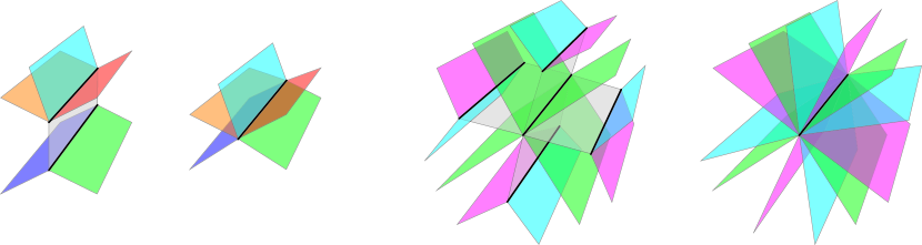
Figure 1. IX-moves and XI-moves: an IX-move along an normal annulus region and an XI-move at an normal branch locus (left), an IX-move along a quasi-normal annulus region and an XI-move at an unnormal branch locus (right).

By an XI-move, a new normal or quasi-normal annulus region, or a new normal Möbius band region arises. An IX-move is uniquely determined up to isotopy for a given normal or quasi-normal annulus region, or a given normal Möbius band region. An XI-move, however, is not uniquely determined for an spreadable branch locus. Note that a branch locus admits an XI-move if and only if it is spreadable. Suppose the region $A$ above is maximally spread. Note that each component (branch locus) of $\partial A$ does not admit XI-moves. Perform the IX-move along $A$. Then the resulting new branch locus admits exactly two XI-moves. One is the reverse operation of the IX-move. A $($$2$-dimensional$)$ IH-move along $A$ is a composition of the IX-move along $A$ and the other XI-move at the new branch locus, see Figure 2.

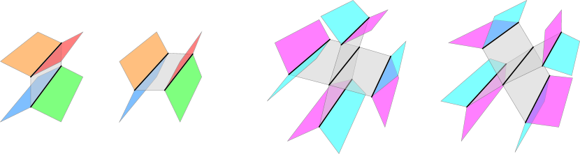
Figure 2. IH-moves: IH-moves along normal maximally spread annulus (or Möbius band) regions (left), IH-moves along quasi-normal maximally spread annulus regions (right).

These moves invariant regular neighborhoods of the mutibranched surfaces up to isotopy. The following is our main theorem, which implies that the converse is also true.

Theorem 1.

Let $X,X^{\prime}$ be multibranched surfaces in an orientable $3$-manifold $M$, and let $N,N^{\prime}$ be their regular neighborhoods respectively. If $N$ is isotopic to $N^{\prime}$ in $M$, then $X$ is transformed into $X^{\prime}$ by a finite sequence of IX-moves, XI-moves and isotopies.

2. Proof of Theorem 1

To prove Theorem 1 we may assume that $N=N^{\prime}$, namely $X^{\prime}$ is in $N$ so that $N$ is also a regular neighborhood of $X^{\prime}$. The characteristic annulus system $\mathcal{A}_{X}$ $($resp. $\mathcal{A}_{X^{\prime}})$ with respect to $X$ (resp. $X^{\prime}$) is the system of mutually disjoint annuli properly embedded in $N$ consisting of $\widehat{C}\times[-1,1]$ for each component $C$ of $\partial S$, where $\widehat{C}$ is in Int($S$) and parallel to $C$ in $S$. The system $\mathcal{A}_{X}$ splits $N$ into pieces $N_{i}$ ($i=1,\ldots,m+n$), where $N_{i}$ is a regular neighborhoods of a branch locus $B_{i}$ of $X$ for $i\in\{1,\ldots,m\}$, and $N_{m+j}$ is homeomorphic to $S_{j}\times[-1,1]$ or $S_{j}\tilde{\times}[-1,1]$ according to whether $S_{j}$ is orientable or not for $j\in\{1,\ldots,n\}$. In other words, $N$ is obtained by attaching $\bigcup_{1\leq j\leq n}N_{m+j}$ to the union $\bigcup_{1\leq i\leq m}N_{i}$ of the solid tori along $\partial S\times[-1,1]$.

An IX-move along a region $A$ of a multibranched surface $X$ in $N$ corresponds to an operation removing one or two annuli $\partial A\times[-1,1]$ from $\mathcal{A}_{X}$ according to whether $A$ is a (normal) Möbius-band region or a (normal/quasi-normal) annulus region. On the other hand, an IX-move in $N$ corresponds to an operation adding two parallel annuli in a solid torus $N_{i}$ ($i\in\{1,\ldots,m\}$) to $\mathcal{A}_{X}$. Note that each spreadable branch locus of $X$ admits an XI-move. By applying XI-moves to $X$ (resp. $X^{\prime}$) maximally, we get a multibranched surface with the non-spreadable branch loci. We call such a multibranched surface a maximally spread surface. Theorem 1 then follows from Theorem 2 below.

Theorem 2.

Let $X$ and $X^{\prime}$ be maximally spread surfaces in $N$ such that $N$ is a regular neighborhood of each of $X$ and $X^{\prime}$. Then $X$ is transformed into $X^{\prime}$ by a finite sequence of IH-moves and isotopies.

Let $\mathcal{A}_{X}$ and $\mathcal{A}_{X^{\prime}}$ be the characteristic annulus system with respect to $X$ and $X^{\prime}$, respectively. We assume that the annuli of $\mathcal{A}_{X}$ and $\mathcal{A}_{X^{\prime}}$ intersect transversely and minimally up to isotopy. If $(\bigcup_{A\in\mathcal{A}_{X}}A)\cap(\bigcup_{A^{\prime}\in\mathcal{A}_{X^{\prime}}}A^{\prime})=\emptyset$, then $X$ and $X^{\prime}$ are isotopic in $N$ since $\mathcal{A}_{X}$ coincides with $\mathcal{A}_{X^{\prime}}$ up to isotopy. Hence we suppose that $(\bigcup_{A\in\mathcal{A}_{X}}A)\cap(\bigcup_{A^{\prime}\in\mathcal{A}_{X^{\prime}}}A^{\prime})\neq\emptyset$.

Claim 1.

Any component $\alpha$ of the intersection between $A\in\mathcal{A}_{X}$ and $A^{\prime}\in\mathcal{A}_{X^{\prime}}$ is an loop and essential in each of $A$ and $A^{\prime}$.

Proof.

First, suppose that $\alpha$ is a loop and inessential in $A$ or $A^{\prime}$, say in $A^{\prime}$. We may assume that $\alpha$ is innermost in $A^{\prime}$. Then the disk $D^{\prime}$ in $A^{\prime}$ bounded by $\alpha$ is in some piece $N_{i}$ ($i\in\{1,\ldots,m+n\}$). Since the core of $A$ is not null-homologous in $N_{i}$, $\alpha$ is also inessential in $A$. Thus $\alpha$ can be removed by isotopy in $N$, which is a contradiction. Next, suppose that $\alpha$ is an arc and inessential in $A$ or $A^{\prime}$, say in $A^{\prime}$. We may assume that $\alpha$ is an outermost arc in $A^{\prime}$. The disk $D^{\prime}$ cut off from $A^{\prime}$ by $\alpha$ is in some piece $N_{i}$ ($i\in\{1,\ldots,m+n\}$). Then $\alpha$ is also inessential in $A$, and so can be removed by isotopy in $N$, a contradiction. Finally, suppose that $\alpha$ is an arc and essential in each of $A$ and $A^{\prime}$. Let $D^{\prime}$ be the component of $A^{\prime}$ cut off by $A\in\mathcal{A}$ such that $\alpha\subset\partial D$ and $D^{\prime}$ lies in some solid torus $N_{i}$ ($i\in\{1,\ldots,m\}$). $\partial D^{\prime}$ intersects $A\in\mathcal{A}$ in two essential arcs in $A^{\prime}$. This implies the degree $d_{i}$ of $B_{i}$ is $2$, that is a contradiction. ∎

By Claim 1, each component of $(\bigcup_{A\in\mathcal{A}_{X}}A)\cap(\bigcup_{A^{\prime}\in\mathcal{A}_{X^{\prime}}}A^{\prime})$ is a loop essential both in $\bigcup_{A\in\mathcal{A}_{X}}A$ and $\bigcup_{A^{\prime}\in\mathcal{A}_{X^{\prime}}}A^{\prime}$. For such systems $\mathcal{A},\mathcal{A^{\prime}}$ of annuli in $N$, we denote by $I(\mathcal{A},\mathcal{A^{\prime}})$ the number of components of the intersection $(\bigcup_{A\in\mathcal{A}}A)\cap(\bigcup_{A^{\prime}\in\mathcal{A^{\prime}}}A^{\prime})$, and by $End(\mathcal{A^{\prime}}|\mathcal{A})$ the set of outermost annuli cut off from annuli in $\mathcal{A^{\prime}}$ along loop intersections. Put $E(\mathcal{A^{\prime}}|\mathcal{A}):=|End(\mathcal{A^{\prime}}|\mathcal{A})|$. We will prove Theorem 2 by induction on the complexity $(E(\mathcal{A}_{X^{\prime}}|\mathcal{A}_{X}),I(\mathcal{A}_{X^{\prime}},\mathcal{A}_{X}))$ in the lexicographic order. Each annulus of $\mathcal{A}_{X^{\prime}}$ having nonempty intersection with annuli of $\mathcal{A}_{X}$ contains exact two elements of $End(\mathcal{A_{A^{\prime}}}|\mathcal{A}_{X})$, so $E(\mathcal{A}_{X^{\prime}}|\mathcal{A}_{X})$ is twice the number of such annuli of $\mathcal{A}_{X^{\prime}}$. We may assume that any annuli of $\mathcal{A}_{X^{\prime}}$ without intersection have been moved into $\bigcup_{j}N_{m+j}$. Take an element $E$ of $End(\mathcal{A}_{X^{\prime}}|\mathcal{A}_{X})$, say, $E\subset A^{\prime}_{1}\in\mathcal{A}_{X^{\prime}}$, $E\cap(\bigcup_{A\in\mathcal{A}_{X}}A)=\partial E\cap A_{1}=\alpha$, and $\beta=\partial E-\alpha$. For $i\in\{1,\ldots,m\}$, we say that the solid torus $N_{i}$ is normal or pure if $B_{i}$ is so.

Claim 2.

$E$ is in an normal solid torus, say $N_{1}$.

Proof.

Suppose that $E$ is in $N_{m+j}$ ($j\in\{1,\ldots,n\}$). Recall that $N_{m+j}$ is homeomorphic to $S_{j}\times[-1,1]$ or $S_{j}\tilde{\times}[-1,1]$. Since $\alpha$ is in $\partial S_{j}\times[-1,1]$ or $S_{j}\tilde{\times}[-1,1]$ and $\beta$ is in $S_{j}\times\{-1,1\}$ or $S_{j}\tilde{\times}\{-1,1\}$, the intersection $\alpha$ can be removed by isotopy in $N$. This is a contradiction. Thus $E$ is in some solid torus, say $N_{1}$. The union $\alpha\cup\beta$ is a $(2d_{1},2e_{1})$-torus link in $\partial N_{1}$, where $d_{1}$ and $e_{1}$ are relative prime integers. The annulus $E$ bounded by $\alpha\cup\beta$ is boundary-parallel in $N_{1}$. If $\partial N_{1}$ contains no annulus of $\mathcal{A}_{X}$ other than the annulus containing $\alpha$, the intersection $\alpha$ can be removed by isotopy in $N$. This is again a contradiction. Hence $\partial N_{1}$ contains more than two annuli of $\mathcal{A}_{X}$. This implies that $N_{1}$ is not pure, thus it is normal. ∎

Let $A_{2},A_{3}$ be the annuli of $\mathcal{A}_{X}$ lying in $\partial N_{1}$ other than $A_{1}$. See Figure 3.

Figure 3. The normal solid torus $N_{1}$.

Claim 3.

$I(\mathcal{A}_{X^{\prime}},\{A_{1}\})>I(\mathcal{A}_{X^{\prime}},\{A_{2}\})+I(\mathcal{A}_{X^{\prime}},\{A_{3}\})$.

Proof.

Let $\tilde{A}_{1},\tilde{A}_{2},\tilde{A}_{3}$ be components of the closure of $\partial N_{1}-(A_{1}\cup A_{2}\cup A_{3})$ such that $\tilde{A}_{i}$ and $A_{i}$ are disjoint for each $i\in\{1,2,3\}$. Let $b_{jk}$ (resp. $b_{jj}$) be the number of (annulus) components of $(\bigcup_{A^{\prime}\in\mathcal{A}_{X^{\prime}}}A^{\prime})\cap N_{1}$ whose boundary lies in $A_{j}\cup A_{k}$ for $j\neq k$ (resp. $A_{j}\cup\tilde{A}_{j}$ for each $j\in\{1,2,3\}$). Then $I(\mathcal{A}_{X^{\prime}},\{A_{j}\})=\sum_{k}b_{jk}$ for each $j\in\{1,2,3\}$. The annulus $E$ with boundaries $\alpha\in A_{1}$, $\beta\in\tilde{A}_{1}$ is counted in $b_{11}$, and so $b_{11}>0$. Any annulus component of $(\bigcup_{A^{\prime}\in\mathcal{A}_{X^{\prime}}}A^{\prime})\cap N_{1}$ other than $E$ has to be contained in one of the two components of $N_{1}-E$, otherwise intersects $E$. Thus we have $b_{22}=b_{33}=b_{23}=0$. Further, we have $I(\mathcal{A}_{X^{\prime}},\{A_{1}\})=b_{11}+b_{12}+b_{13}=b_{11}+I(\mathcal{A}_{X^{\prime}},\{A_{2}\})+I(\mathcal{A}_{X^{\prime}},\{A_{3}\})>I(\mathcal{A}_{X^{\prime}},\{A_{2}\})+I(\mathcal{A}_{X^{\prime}},\{A_{3}\})$. ∎

We may assume that $A_{1}\subset N_{1}\cap N_{m+1}$. Recall that the piece $N_{m+1}$ corresponds to the region $S_{1}$, which is an normal Möbius band region, normal annulus region, quasi-normal annulus region or closing annulus region. Here we know $S_{1}$ is neither an unnormal Möbius band region nor an unnormal annulus region since $B_{1}$ is normal by Claim 2.

Claim 4.

$S_{1}$ is not a closing annulus region.

Proof.

Suppose that $S_{1}$ is a closing annulus region. It means that $N_{1}\cap N_{m+1}=A_{1}\cup A_{2}$ or $A_{1}\cup A_{3}$, say, $A_{1}\cup A_{2}$. Two boundary components of each annulus component of $(\bigcup_{A^{\prime}\in\mathcal{A}_{X^{\prime}}}A^{\prime})\cap N_{m+1}$ must lie $A_{1}$ and $A_{2}$, respectively. Then $I(\mathcal{A}_{X^{\prime}},\{A_{1}\})=I(\mathcal{A}_{X^{\prime}},\{A_{2}\})$, that contradicts Claim 3. ∎

If $S_{1}$ is an normal Möbius band region, let $N_{12}$ be the solid torus $N_{1}\cup N_{m+1}$. If $S_{1}$ is an annulus region, by Claim 4, $\partial S_{1}$ has one branch locus other than $B_{1}$, say, $B_{2}$, so let $N_{12}$ be the solid torus $N_{1}\cup N_{m+1}\cup N_{2}$, and put $A_{4}:=N_{2}\cap N_{m+1}$, which is an annulus of $\mathcal{A}_{X}$. Consider the maximally spread surface $X^{(1)}$ obtained from $X$ by an IH-move along $S_{1}$. If $S_{1}$ is an normal Möbius band region, the characteristic annulus system $\mathcal{A}_{X^{(1)}}$ with respect to $X^{(1)}$ is obtained from $\mathcal{A}_{X}$ by replacing $A_{1}$ with an annulus $A_{1}^{(1)}$ in $N_{12}$ disjoint from any annuli of $\mathcal{A}_{X}-\{A_{1}\}$. See Figure 4.

Figure 4. The IH-move along $S_{1}$ when $S_{1}$ is an normal Möbius-band region.

If, on the other hand, $S_{1}$ is an normal or quasi-normal annulus region, the characteristic annulus system $\mathcal{A}_{X^{(1)}}$ with respect to $X^{(1)}$ is obtained from $\mathcal{A}_{X}$ by replacing $\{A_{1},A_{4}\}$ with parallel annuli $\{A_{1}^{(1)},A_{4}^{(1)}\}$ in $N_{12}$ disjoint from any annuli of $\mathcal{A}_{X}-\{A_{1},A_{4}\}$. See Figure 4.

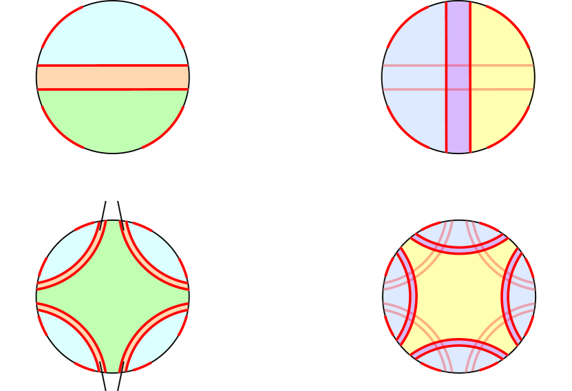
Figure 5. The IH-move along $S_{1}$ when $S_{1}$ is an normal or quasi-normal annulus region.

Let $E^{*}$ be the component of $A^{\prime}_{1}\cap N_{12}$ which contains the annulus $E$ and $\gamma=\partial E^{*}-\beta$. Then exactly one of the following holds:

:

Case $1$: $E^{*}=A^{\prime}_{1}$, see Figure 6.

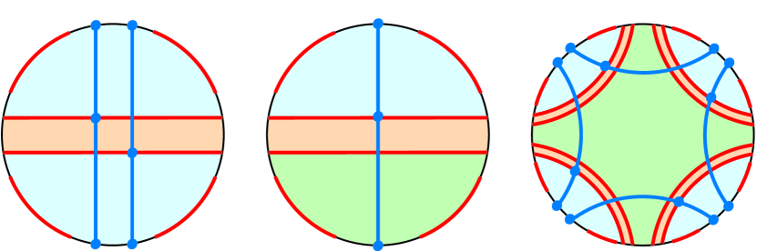
Figure 6. The annulus $E^{*}$ in Case 1 when $S_{1}$ is (i) an normal Möbius-band region; (ii) an normal annulus region; (iii) a quasi-normal annulus region.

:

Case $2$: $E^{*}\neq A^{\prime}_{1}$ and $S_{1}$ is an normal Möbius-band region or a quasi-normal annulus region, see Figure 7.

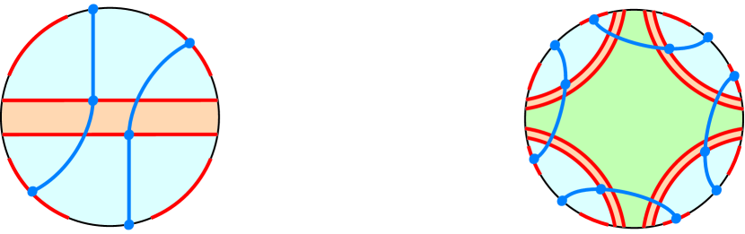
Figure 7. The annulus $E^{*}$ in Case 2 when $S_{1}$ is (i) an normal Möbius-band region; (ii) an annulus region.

:

Case $3$: $E^{*}\neq A^{\prime}_{1}$ and $S_{1}$ is an normal annulus region, see Figure 8.

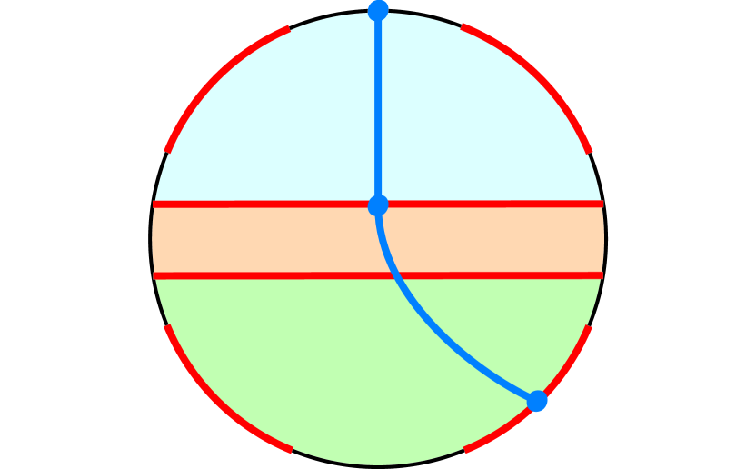
Figure 8. The annulus $E^{*}$ in Case 3.

Claim 5.

In Case $1$, we have $E(\mathcal{A}_{X^{\prime}}|\mathcal{A}_{X^{(1)}})<E(\mathcal{A}_{X^{\prime}}|\mathcal{A}_{X})$.

Proof.

The annuli $A_{1}^{(1)}$ (and $A_{4}^{(1)}$ as well if $S_{1}$ is an annulus region) are isotopic to $E^{*}=A^{\prime}_{1}$ in $N$. Then $End(\mathcal{A}_{X^{\prime}}|\mathcal{A}_{X^{(1)}})\subset End(\mathcal{A}_{X^{\prime}}|\mathcal{A}_{X})$ and $E\in End(\mathcal{A}_{X^{\prime}}|\mathcal{A}_{X})-End(\mathcal{A}_{X^{\prime}}|\mathcal{A}_{X^{(1)}})$. Hence $E(\mathcal{A}_{X^{\prime}}|\mathcal{A}_{X^{(1)}})<E(\mathcal{A}_{X^{\prime}}|\mathcal{A}_{X})$. ∎

For Case $2$, since $A_{2}$ and $A_{3}$ are the only annuli of $\mathcal{A}_{X}$ lying in $\partial N_{12}$, the loop $\gamma$ lies in $A_{2}$ or $A_{3}$, say, $A_{2}$.

Claim 6.

In Case $2$, we have $E(\mathcal{A}_{X^{\prime}}|\mathcal{A}_{X^{(1)}})\leq E(\mathcal{A}_{X^{\prime}}|\mathcal{A}_{X})$, $I(\mathcal{A}_{X^{\prime}},\{A_{1}^{(1)}\})<I(\mathcal{A}_{X^{\prime}},\{A_{2}\})$ and $I(\mathcal{A}_{X^{\prime}},\mathcal{A}_{X^{(1)}})<I(\mathcal{A}_{X^{\prime}},\mathcal{A}_{X})$ in Case $2$.

Proof.

The annulus $A_{2}$ is divided into two annuli by $\gamma$. One of the annuli, denoted by $F$, makes the annulus $E^{*}\cup F$ isotopic to $A_{1}^{(1)}$ in $N$. Then each annulus of $\mathcal{A}_{X^{\prime}}$ that intersects annuli of $\mathcal{A}_{X^{(1)}}$ must intersect annuli of $\mathcal{A}_{X}$. This implies that $E(\mathcal{A}_{X^{\prime}}|\mathcal{A}_{X^{(1)}})\leq E(\mathcal{A}_{X^{\prime}}|\mathcal{A}_{X})$. Since $F$ is contained in $A_{2}$, $I(\mathcal{A}_{X^{\prime}},\{A_{1}^{(1)}\})<I(\mathcal{A}_{X^{\prime}},\{A_{2}\})$. By Claim 3, we have $I(\mathcal{A}_{X^{\prime}},\{A_{1}^{(1)}\})<I(\mathcal{A}_{X^{\prime}},\{A_{1}\})$. If $S_{1}$ is an annulus region, $I(\mathcal{A}_{X^{\prime}},\{A_{4}^{(1)}\})<I(\mathcal{A}_{X^{\prime}},\{A_{4}\})$ since the two annuli $A_{1}$ and $A_{4}$ (resp. $A_{1}^{(1)}$ and $A_{4}^{(1)}$) are parallel. Hence we have $I(\mathcal{A}_{X^{\prime}},\mathcal{A}_{X^{(1)}})<I(\mathcal{A}_{X^{\prime}},\mathcal{A}_{X})$. ∎

For Case $3$, let $A_{5},A_{6}$ be the annuli of $\mathcal{A}_{X}$ lying in $\partial N_{2}$ other than $A_{4}$ so that $\gamma\subset A_{5}$. By the same argument in the proof of Claim 6, we have the following.

Claim 7.

In Case $3$, we have $E(\mathcal{A}_{X^{\prime}}|\mathcal{A}_{X^{(1)}})\leq E(\mathcal{A}_{X^{\prime}}|\mathcal{A}_{X})$ and $I(\mathcal{A}_{X^{\prime}},\{A_{1}^{(1)}\})=I(\mathcal{A}_{X^{\prime}},\{A_{4}^{(1)}\})<I(\mathcal{A}_{X^{\prime}},\{A_{5}\})$.

Claim 8.

The complexity $I(\mathcal{A}_{X^{\prime}},\mathcal{A}_{X})$ decreases after a finite sequence of IH-moves for $\mathcal{A}_{X^{\prime}}$.

Proof.

By Claims 5 and 6, the complexity $I(\mathcal{A}_{X^{\prime}},\mathcal{A}_{X})$ decreases after performing the IH-move along $S_{1}$, so we are done. The complexity $I(\mathcal{A}_{X^{\prime}},\mathcal{A}_{X})$ may increase after the IH-move along $S_{1}$ in Case $3$. By the same argument as in Luo [8], however, we conclude that the complexity $(E(\mathcal{A}_{X^{\prime}}|\mathcal{A}_{X}),I(\mathcal{A}_{X^{\prime}},\mathcal{A}_{X}))$ is reduced after a finite number of IH-moves as follows. The annulus $E^{*}$ in Case $3$ as well as in Case $2$ is an element of $End(\mathcal{A}_{X^{\prime}}|\mathcal{A}_{X^{(1)}})$. We repeat the same argument using the annulus $E^{*}$ among annuli of $End(\mathcal{A}_{X^{\prime}}|\mathcal{A}_{X^{(1)}})$. If Case $1$ occurs for $E^{*}$, the complexity decreases, so we are done. Therefore, it remains to show that after repeating the same process (IH-moves) finitely many times, we finally get an outer most annulus of Case $1$. To prove this, let us exam the change in the $n$-tuple $(a_{1},\dots,a_{n})$ of non-negative integers

$$a_{j}=\left\{\begin{array}[]{ll}\frac{1}{2}I(\mathcal{A}_{X^{\prime}},\mathcal{A}_{S_{j}})&\mbox{if $S_{j}$ is an annulus region},\\ I(\mathcal{A}_{X^{\prime}},\mathcal{A}_{S_{j}})&\mbox{otherwise},\end{array}\right.$$

where $\mathcal{A}_{S_{j}}$ is the set of all annuli lying in $\partial N_{m+j}$. By Claims 6 and 7, at the first step (i.e. the IH-move along $S_{1}$), we replace one coordinate of the $n$-tuple $(a_{1},\dots,a_{n})$, say $a_{i_{0}}$, by $a_{i_{0}}^{(1)}$, where $0\leq a_{i_{0}}^{(1)}\leq a_{i_{1}}-1$ for some $i_{1}\neq i_{0}$. Let the new $n$-tuple thus obtained be $(a_{1}^{(1)},\dots,a_{n}^{(1)})$. Now we replace $a_{i_{1}}^{(1)}$ by $a_{i_{1}}^{(2)}$, where $0\leq a_{i_{1}}^{(2)}\leq a_{i_{2}}^{(1)}-1$ for some $i_{2}\neq i_{1}$. Suppose in the $k$-th step we obtain the $n$-tuple $(a_{1}^{(k)},\dots,a_{n}^{(k)})$, where $0\leq a_{i_{k-1}}^{(k)}\leq a_{i_{k}}^{(k-1)}-1$. Noting that $a_{i_{k}}^{(k-1)}=a_{i_{k}}^{(k)}$, we have

$$\sum_{i=1}^{n}a_{i}^{(k)} = \sum_{i=1}^{n}a_{i}^{(k-1)}-a_{i_{k-1}}^{(k-1)}+a_{i_{k}}^{(k)}$$

$$\leq \sum_{i=1}^{n}a_{i}^{(k-1)}-a_{i_{k-1}}^{(k-1)}+a_{i_{k}}^{(k-1)}-1$$

$$= \sum_{i=1}^{n}a_{i}^{(k-1)}-a_{i_{k-1}}^{(k-1)}+a_{i_{k}}^{(k)}-1.$$

By the construction, it holds $0\leq a_{i}^{(k)}\leq\max\{a_{1},\ldots,a_{n}\}-1$ for all $k$ and $i$. Thus from the above inequality, it follows that

$$\sum_{i=1}^{n}a_{i}^{(k)} \leq \sum_{i=1}^{n}a_{i}^{(k-1)}-a_{i_{k-1}}^{(k-1)}+a_{i_{k}}^{(k)}-1$$

$$\leq \sum_{i=1}^{n}a_{i}^{(k-2)}-a_{i_{k-2}}^{(k-2)}+a_{i_{k}}^{(k)}-2$$

$$\leq \cdots$$

$$\leq \sum_{i=1}^{n}a_{i}-a_{i_{0}}+a_{i_{k}}^{(k)}-k$$

$$\leq \sum_{i=1}^{n}a_{i}+\max\{a_{1},\ldots,a_{n}\}-k-1.$$

Hence after at most $(\sum_{i=1}^{n}a_{i}+\max\{a_{1},\ldots,a_{n}\})$ steps, the $n$-tuple becomes the zero vector $(0,\ldots,0)$. This implies that the complexity decreases after performing a finite sequence of IH-moves. ∎

Claim 8 completes the induction step and hence the proof of Theorem 2.

3. Poly-continuous patterns and networks

One background of this study is constructing a mathematical model of structures made by diblock or triblock copolymers.

Diblock copolymers produces spherical, cylindrical, lamellar and bicontinuous structures. See [10] for example. Typical examples of bicontinuous structures are Gyroid, D-surface and P-surface[14]. Mathematical model of such structures are triply periodic non-compact surfaces $F$ embedded in $\mathbb{R}^{3}$ which divide $\mathbb{R}^{3}$ into two possibly disconnected submanifolds $V_{1}$ and $V_{2}$ such that $V_{1}\cap V_{2}=\partial V_{1}\cap\partial V_{2}=F$. A subset of $\mathbb{R}^{3}$ is called triply periodic if it is invariant by the standard $\mathbb{Z}^{3}$ action on $\mathbb{R}^{3}$. We call such a surface a bicontinuous pattern [6].

We will consider the case where $V_{1}$ and $V_{2}$ are open neighborhood of networks. Here a network means an infinite graph embedded in $\mathbb{R}^{3}$. See, for example, [6, 5]. In this case the bicontinuous pattern is uniquely determined by networks up to isotopy. We say such a bicontinuous pattern is associated to a network.

On the other hand, for example triblock-arm star-shaped molecules yields a tricontinuous structure [1]. One mathematical model of such tricontinuous (resp. poly-continuous) structures is a triply periodic non-compact multibranched surface (or more generally polyhedron) dividing $\mathbb{R}^{3}$ into 3 (resp. several) possibly disconnected non-compact submanifolds $V_{1}$, $V_{2}$ and $V_{3}$ (resp. $V_{1},\cdots,V_{k}$). We assume that each $V_{i}$ is the open neighborhood of three (resp. several) networks in $\mathbb{R}^{3}$. We call such a multibranched surface a tricontinuous pattern (resp. poly-continuous pattern)[6, 5, 15].

The relation between poly-continuous patterns and networks is not obvious in this case. Two different poly-continuous patterns are associated to one network and vice versa. Here we will give a necessary and sufficient condition for poly-cotinuous patterns to give the same network.

By considering the quotient space of the standard $\mathbb{Z}^{3}$ action, we obtain a graph in the 3-dimensional torus $T^{3}$ as the quotient space of the triply periodic network and a compact multibranched surface in $T^{3}$ as the quotient space of the triply periodic poly-continuous pattern.

IX-moves and XI-moves for triply periodic poly-continuous patterns in $\mathbb{R}^{3}$ are lifts of IX-moves and XI-moves of the corresponding multibranched surfaces in $T^{3}$, By applying Theorem 1, two multibranched surfaces in $T^{3}$ corresponding to two poly-continuous pattern of a given triply periodic network can be related by a finite sequence of IX-moves, XI-moves and isotopies.

Theorem 3.

Let $X$ and $X^{\prime}$ be triply periodic poly-continuous patterns in $\mathbb{R}^{3}$ associated to a triply periodic network of multiple components. Suppose that $X$ and $X^{\prime}$ have no disk region. Then $X$ can be transformed into $X^{\prime}$ by a finite sequence of $IX$-moves, $XI$-moves and isotopies.

By applying [9], two networks corresponding to one triply periodic poly-continuous pattern can be related by a finite sequence of lifts of edge-contractions and vertex-expansions of quotient graphs in $T^{3}$.

Study of tricontinuous patterns using decomposition of $T^{3}$ with a multibranched surface will be discussed in the forthcoming papers [17].

4. A short remark on minors of multibranched surfaces

As an analogy of graph minor (e.g. [2]), Matsuzaki and the third author introduced the notion of minor of multibranched surfaces and studied intrinsic properties of multibranched surfaces ([11]). However, in that paper, the authors took into consideration only IX-moves along normal annulus regions. Based on Theorem 1, it is more natural to define the minor of multibranched surfaces as follows. In this section, we allow the degree $d_{i}$ of a branch locus $B_{i}$ to be $1$ or $2$ as well, and we assume that a multibranched surface is regular (i.e. for each branch locus $B_{i}$, the wrapping number of all components of $f^{-1}(B_{i})$ is a divisor of the degree $d_{i}$ of $B_{i}$.

We consider regular multibranched surfaces modulo homeomorphism. Let $X$ and $Y$ be regular multibranched surfaces. We write $X\overset{\mathrm{r}}{<}Y$ if $X$ is obtained by removing a region of $Y$. We write $X\overset{\mathrm{c}}{<}Y$ if $X$ is obtained by contracting an normal annulus region, a quasi-normal annulus region or an normal Möbius-band region of $Y$. If $X\overset{\mathrm{r}}{<}Y$ or $X\overset{\mathrm{c}}{<}Y$, we write $X<Y$.

We denote by $\mathcal{M}$ the set of all regular multibranched surfaces (modulo homeomorphism). We define an equivalence relation $\sim$ on $\mathcal{M}$ as follows: if $X<Y$ and $Y<X$, then $X\sim Y$. An element of the quotient set $\mathcal{M}/\sim$ is called a multibranched surface class (or a multibranched surface for simplicity). We define a partial order $\prec$ on $\mathcal{M}/\sim$ as follows. Let $X$, $Y\in\mathcal{M}$. We denote $[X]\prec[Y]$ if there exists a finite sequence $X_{0},X_{1},\ldots,X_{n-1},X_{n}$ of multibranched surfaces such that $X_{0}\sim X$, $X_{n}\sim Y$ and $X_{0}<X_{1}<\cdots<X_{n-1}<X_{n}$.

A multibranched surface (class) $[X]$ is called a minor of a multibranched surface (class) $[Y]$ if $[X]\prec[Y]$. In particular, $[X]$ is called a proper minor of $[Y]$ if $[X]\prec[Y]$ and $[Y]\not=[X]$. A subset $\mathcal{P}$ of $\mathcal{M}/\sim$ is said to be minor closed if for every multibranched surface $[X]\in\mathcal{P}$, every minor of $[X]$ belongs to $\mathcal{P}$. For a minor closed set $\mathcal{P}$, we define the obstruction set $\Omega(\mathcal{P})$ as follows:

$$\Omega(\mathcal{P})=\left\{[X]\in\mathcal{M}/\sim\mid[X]\not\in\mathcal{P},\mbox{ Every proper minor of }[X]\mbox{ belongs to }\mathcal{P}.\right\}$$

With respect to the above notion, the results stated in [11] still hold. For example, the set of multibranched surfaces embeddable into $S^{3}$, denoted by $\mathcal{P}{S^{3}}$, is minor closed ([11, Proposition 5.7]), and for a multibranched surface $X$ in Fig. 11 of [11] or equivalently $X=X_{g}(p_{1},p_{2},\ldots,p_{n})$ in [4], if $p={\rm gcd}\{p_{1},p_{2},\ldots,p_{n}\}$ is not $1$, then $X\in\Omega(\mathcal{P}S^{3})$. As the philosophy of graph minor theory, the obstruction set for the embeddability into a 3-manifold reflects the properties of the 3-manifold. Finally, we propose the next problem which can be regarded as a 2-dimensional version of Kuratowski’s and Wagner’s theorems.

Problem 1.

Characterize the obstruction set $\Omega(\mathcal{P}S^{3})$.

It is known that the following multibranched surfaces belong to $\Omega(\mathcal{P}S^{3})$.

• non-orientable closed surfaces.

• $X_{1}$ in [3, Theorem 3.2], where $|ad_{e_{1}}(l_{1})|\geq 2$.

• $X_{2}$ in [3, Theorem 3.3].

• $X_{3}$ in [3, Theorem 3.7].

• $X$ in [11, Example 5.8] or [4], where $p={\rm gcd}\{p_{1},p_{2},\ldots,p_{n}\}\neq 1$.

• $X$ in [11, Example 5.9].

References

• [1] de Campo, L., Castle T., Hyde S. T., Optimal packings of three-arm star polyphiles: from tricontinuous to quasi-uniformly striped bicontinuous forms, Interface Focus 7 (2017) 20160130. http://dx.doi.org/10.1098/rsfs.2016.0130
• [2] R. Diestel, Graph Theory, Graduate Texts in Mathematics, Springer-Verlag, New York, 2000.
• [3] K. Eto, S. Matsuzaki, M. Ozawa, An obstruction to embedding 2-dimensional complexes into the 3-sphere, Topology and its Appl. 198 (2016) 117–125.
• [4] Eudave-Muõz, M., Ozawa, M., Characterization of 3-punctured spheres in non-hyperbolic link exteriors, arXiv:1805.12523.
• [5] Hyde S. T., de Campo. L., Oguey C., Tricontinuous mesophases of balanced three-arm ‘star polyphiles’, Soft Matter, 5, 2782-2794, (2009).
• [6] Hyde S. T., Ramsden, S., Polycontinuous morphologies and interwoven helical networks, Europhys. Lett., 50 (2), pp. 135-141 (2000).
• [7] Ishii, A., Moves and invariants for knotted handlebodies, Algebr. Geom. Topol. 8 (2008), no. 3, 1403–1418.
• [8] Luo, F., On Heegaard diagrams, Math. Res. Lett. 4 (1997), no. 2–3, 365–373.
• [9] Makino, K., Suzuki, S., Notes on neighborhood congruence of spatial graphs, Gakujutu Kenkyu, School of Education, Waseda Univ. Ser. Math., 43 (1995), 15–20.
• [10] Matsen, M. W., Effect of Architecture on the Phase Behavior of AB-Type Block Copolymer Melts, Macromolecules 45 (4), (2012), 2161-2165. DOI: 10.1021/ma202782s
• [11] Matsuzaki, S., Ozawa, M., Genera and minors of multibranched surfaces, Topology and its Appl. 230 (2017), 621–638.
• [12] Matveev, S. V., Transformations of special spines and the Zeeman conjecture, Math. USSR-Izv. 31 (1988), no. 2, 423–434.
• [13] Piergallini, R., Standard moves for standard polyhedra and spines, Rend. Circ. Mat. Palermo (2) Suppl. No. 18 (1988), 391–414.
• [14] Squires, A. M., Templer, R. H., Seddon J. M., Woenkhaus, J., Winter, R., Narayanan, T., Finet, S., Kinetics and mechanism of the interconversion of inverse bicontinuous cubic mesophases, Phys. Rev. E 72, (2005) 011502.
• [15] Schröder-Turk, G. E., de Campo, L., Evans, M. E., Saba, M., Kapfer, S., Varslot T., Grosse-Brauckmann, K., Ramsden, S., Hyde S., Polycontinuous geometries for inverse lipid phases with more than two aqueous network domains, Faraday Discuss. 161, 215-247 10.1039/C2FD20112G (2012)
• [16] Suzuki, S., On linear graphs in $3$-sphere, Osaka J. Math. 7 1970, 375–396.
• [17] In preparation.