Abstract

The concept of observability of linear systems initiated with Kalman in the mid 1950s. Roughly a decade later, the observability of nonlinear systems appeared. By such definitions a system is either observable or not. Continuous measures of observability for linear systems were proposed in the 1970s and two decades ago were adapted to deal with nonlinear dynamical systems. Related topics developed either independently or as a consequence of these. Observability has been recognized as an important feature to study complex networks, but as for dynamical systems in the beginning the focus has been on determining conditions for a network to be observable. In this relatively new field previous and new results on observability merge either producing new terminology or using terms, with well established meaning in other fields, to refer to new concepts. Motivated by the fact that twenty years have passed since some of these concepts were introduced in the field of nonlinear dynamics, in this paper (i) various aspects of observability will be reviewed, and (ii) it will be discussed in which ways networks could be ranked in terms of observability. The aim is to make a clear distinction between concepts and to understand what does each one contribute to the analysis and monitoring of networks. Some of the main ideas are illustrated with simulations.

1 Introduction

One of the many concepts used to analyze dynamical systems and networks is observability. The genesis of this can be traced back to mid 20th century. It is interesting to see that depending on the research area observability has been painted with different colors. In control theory, the cradle of this concept [Kalman, 1960], observability is related to the ability of reconstructing the state of the system from a limited set of measured variables in finite time. A somewhat relaxed version of this definition of observability and which is applicable to networks is known as structural observability and can be assessed with graph [Lin, 1974]. These concepts have a main aspect in common: both classify the system as either being observable or not. In this paper the term structural observability  will be used to refer to such a feature. In the case of networks such concepts could, in principle, be used to decide how many nodes should be measured in order to render the network observable.

There is a different approach to observability, which evolved from the traditional one, that has a different aim. Even if a system is observable, it might be advantageous, especially from a numerical point of view, to measure specific variables. Instead of a crisp classification in terms of observability, this concept permits distinguishing between more and less observable scenarios [Friedland, 1975, Aguirre, 1995]. We shall refer to this as dynamical observability. Two decades ago, some of these concepts were adapted to rank variables of nonlinear dynamical systems based on observability [Letellier et al., 1998] and from there appeared other related approaches that will be briefly reviewed in this work.

In the context of networks, the concepts of observability and its dual – controllability – have been recognized as relevant tools for analysis and design [Liu et al., 2013, Whalen et al., 2015, Su et al., 2017, Leitold et al., 2017, Haber et al, 2017]. In this respect, two aspects stand out. First, the classical procedures to determine if a system is observable face some serious practical and numerical difficulties when applied to larger systems. Indeed, it seems that in the case of high-dimensional network, most often the observability is only investigated from its topology (described by the adjacency matrix): this will be referred to as topological observability  in this paper. As it will be shown, in a network in which oscillators are connected according to an adjacency matrix, investigating its connectivity of the corresponding graph is not sufficient in general to assess the observability of the network. Second, to determine a minimum number of sensor nodes for which a network is observable is a valuable piece of information. But to be able to choose from alternative configurations seems to be an important step forward that still has to be accomplished.

As it will be argued in this paper, the classical way of classifying systems as being observable or not, cannot really help much in solving the mentioned challenge as recently pointed out [Leitold et al., 2017, Haber et al, 2017, Letellier et al., 2018]. In order to do so, alternative scenarios in which observability is guaranteed must be compared in order to decide which is more favorable. In other words, as it happened for dynamical systems, also for networks there should be a change in paradigm from structural to dynamical observability.

The benefits and need for this has already been pointed out in the literature. For instance, it has been acknowledged that to choose variables that convey good observability of the dynamics enables estimating the state of a network of neuron models using Kalman-related methods [Sedigh-Sarvestani et al., 2012, Schiff, 2012]. In a recent study about controllability and observability of network topologies built with neuron models, it has been found that “it is necessary to take the node dynamics into consideration when selecting the best driver (sensor) node to modulate (observe) the whole network activity” [Su et al., 2017, Sec. III-A]. The reader should notice the need to pick good  observables or to choose the best  sensor nodes. This type of challenge can be met conceptually using dynamical observability. Of course, the numerical challenge of determining such a property for a large network is of paramount importance and, at the moment, seems unsolved in general.

In view of all this, one of the aims of this paper is to review some concepts and procedures concerning observability in the context of nonlinear dynamics. It will be useful to see that observability can be classified into different types. Hopefully this classification will clarify the main differences which could help to answer some of the recent remarks that appeared in the literature. Also, the application of such concepts to networks will be discussed. Even if from a numerical point of view, some procedures are not feasible in the context of large networks, there is much to be gained in conceptual terms. In particular, numerical examples will be provided for showing that dynamical observability is not necessarily related to the network dynamics and that the apparent flow of information can be a purely dynamical effect.

1.1 Terminology and organization

This paper shall refer to dynamical networks as the interconnection of dynamical systems of order greater than one. Such dynamical systems will sometimes be called oscillators and compose the node dynamics of the dynamical network. The interconnection of such nodes is according to a certain topology which is described by the adjacency matrix of the network. Graphs can be defined for: i) the node dynamics, which sometimes are referred to as fluence graphs; ii) the topology, and for iii) the full dynamical network (combining the node dynamics and the network topology).

This paper is organized as follows. Section 2 reviews a number of concepts that underline the rest of the paper concerning observability, especially as they emerged from the field of dynamical systems. The counterpart, in the context of network topologies, is provided in Section 3. Different types or aspects of observability are then summarized in Section 4. Section 5 discusses the relevance of the aforementioned concepts in the case of nonlinear dynamical networks. That section also includes some simulation results. The main points are summarized in Section 6, where Table 1 is provided as a “road map” of this paper.

2 Observability of Dynamical Systems

The objective of this section is to give a brief historical background in order to set the remainder of the paper into context. The main ideas in this section will be illustrated with the paradigmatic Rössler system.

2.1 Either observable or not

The concepts of observability and controllability for linear systems are due to Rudolf Kalman [Kalman, 1960]. Consider the linear system

$$\left\{\begin{array}[]{lcl}\dot{\mbox{\boldmath$x$}}&=&A\mbox{\boldmath$x$}+B\mbox{\boldmath$u$}\\ \mbox{\boldmath$s$}&=&C\mbox{\boldmath$x$},\end{array}\right.$$ (1)

where $\mbox{\boldmath$x$}\in\mbox{\bbfnt R}^{n}$ is the state vector, $\mbox{\boldmath$s$}\in\mbox{\bbfnt R}^{p}$ is the measurement vector, $\mbox{\boldmath$u$}\in\mbox{\bbfnt R}^{r}$ is the input vector and $(A,\,B,\,C)$ are constant matrices known respectively as the dynamics matrix, the input or control matrix and the output or measurement matrix. The system (1) is said to be observable at time $t_{f}$ if the initial state $\mbox{\boldmath$x$}(0)$ can be uniquely determined from knowledge of a finite time history of the output $s(\tau)$, $0\leq\tau\leq t_{f}$ [Chen, 1999] and the input $u(\tau)$ whenever it exists.

One way of testing whether the system (1) is observable is to define the observability matrix:

$${\cal O}=\left[\begin{array}[]{ccccc}C&CA&CA^{2}&\ldots&CA^{n-1}\end{array}\right]^{\scriptscriptstyle\rm T}.$$ (3)

The system (1) is therefore observable if matrix ${\cal O}$ is full rank, that is if its rank $\rho[{\cal O}]=n$. This is known as Kalman’s rank condition for observability and according to it a pair $[A,C]$ is either observable or not.

The concepts of controllability and observability were extended to nonlinear systems in the 1970s, e.g. [Hermann and Krener, 1977]. Consider a nonlinear system

$$\left\{\begin{array}[]{l}\dot{\mbox{\boldmath$x$}}=\mbox{f}(\mbox{\boldmath$x$})\\ s(t)=h(\mbox{\boldmath$x$}),\end{array}\right.$$ (4)

with $\mbox{f}\,:\mbox{\bbfnt R}^{n}\rightarrow\mbox{\bbfnt R}^{n}$ and, for simplicity $s(t)\in\mbox{\bbfnt R}$, that is $h\,:\mbox{\bbfnt R}^{n}\rightarrow\mbox{\bbfnt R}$. Differentiating $s(t)$ yields

$$\dot{s}(t)=\frac{\rm d}{{\rm d}t}h(\mbox{\boldmath$x$})=\frac{\partial h}{\partial\mbox{\boldmath$x$}}\dot{\mbox{\boldmath$x$}}=\frac{\partial h}{\partial\mbox{\boldmath$x$}}\mbox{f}(\mbox{\boldmath$x$})={\cal L}_{f}h(\mbox{\boldmath$x$}).$$ (5)

${\cal L}_{f}h(\mbox{\boldmath$x$})$ is the Lie derivative of $h$ along the vector field f. Hence the time derivatives of $s$ can be written in terms of Lie derivatives as $s^{(j)}={\cal L}^{j}_{f}h(\mbox{\boldmath$x$})$. The $j$th-order Lie derivative is given by

$${\cal L}^{j}_{f}h(\mbox{\boldmath$x$})=\frac{\partial{\cal L}^{j-1}_{f}h(\mbox{\boldmath$x$})}{\partial\mbox{\boldmath$x$}}\cdot\mbox{f}(\mbox{\boldmath$x$})$$ (6)

where ${\cal L}^{0}_{f}h(\mbox{\boldmath$x$})=h(\mbox{\boldmath$x$})$. The observability matrix can be written as

$${\cal O}_{s}(\mbox{\boldmath$x$})=\left[\begin{array}[]{ccc}\displaystyle\frac{\partial{\cal L}^{0}_{f}h(\mbox{\boldmath$x$})}{\partial\mbox{\boldmath$x$}}&\ldots&\displaystyle\frac{\partial{\cal L}^{n-1}_{f}h(\mbox{\boldmath$x$})}{\partial\mbox{\boldmath$x$}}\end{array}\right]^{\scriptscriptstyle\rm T}$$ (7)

where the index $s$ has been used to emphasize that ${\cal O}_{s}(\mbox{\boldmath$x$})$ refers to the system observed from $s(t)$.

The pair $[\mbox{f},h(\mbox{\boldmath$x$})]$ in (4) is said to be observable if $\rho[{\cal O}_{s}(\mbox{\boldmath$x$})]=n,~{}\forall\mbox{\boldmath$x$}\in\mathbb{R}^{n}$, which is the counterpart of Kalman’s rank condition for linear systems – see [Hermann and Krener, 1977] for details. If $[\mbox{f},\,h(\mbox{\boldmath$x$})]$ is observable, any two initial conditions $\mbox{\boldmath$x$}_{0_{1}}$ and $\mbox{\boldmath$x$}_{0_{2}}$ are distinguishable with respect to the measured time series $s(t),~{}t\geq 0$. That is, if the system is observable, it is possible to trace back every single initial condition given only the measured time series $s(t),~{}t\geq 0$, or still, $h(\mbox{\boldmath$x$}_{0_{1}})|_{t\geq 0}\neq h(\mbox{\boldmath$x$}_{0_{2}})|_{t\geq 0}$ if $\mbox{\boldmath$x$}_{0_{1}}\neq\mbox{\boldmath$x$}_{0_{2}}$.

Since observability is determined by a rank criterion in both cases, linear and nonlinear systems are classified either as observable or not.

An interesting step in the field was to recognize that the observability matrix in (7) is in fact the Jacobian matrix of the map

$$\Phi_{s}\,:\mbox{\bbfnt R}^{n}(\mbox{x})\mapsto\mbox{\bbfnt R}^{n}(s(t),s^{(1)},...,s^{(n-1)}),\,$$

between the original and the $n$-dimensional differential embedding spaces [Letellier et al., 2005]. If $\Phi_{s}$ is invertible (injective), it is possible to reconstruct the state from $s(t)$. The condition for invertibility of $\Phi_{s}$ at $\mbox{x}_{0}$ is

$$\rho\left[\left.\displaystyle\frac{\partial\Phi_{s}}{\partial\mbox{x}}\right|_{\mbox{x}=\mbox{x}_{0}}\right]=n.$$ (8)

Hence, the system is locally observable if condition (8) holds, that is, if $\Phi_{s}$ is locally invertible. If $\Phi_{s}$ is constant and invertible, then there is a global diffeomorphism and the pair $[\mbox{f},h]$ is fully observable. When the reconstructed space is $n$-dimensional, and thus $\frac{\partial\Phi_{s}}{\partial\mbox{x}}$ is a $n\times n$ matrix, it may be also useful to express condition (8) as [Letellier and Aguirre, 2002]

$$\mbox{Det }\frac{\partial\Phi_{s}}{\partial\mbox{x}}\neq 0\,.$$ (9)

Remark 2.1

If the dimension of the reconstructed space is allowed to increase using

$$\Phi_{s}\,:\mbox{\bbfnt R}^{n}(\mbox{x})\mapsto\mbox{\bbfnt R}^{d}(s(t),s^{(1)},...,s^{(d-1)})\,,$$

with $d>n$, often, singularities that $\Phi_{s}$ may have will vanish and, then $\Phi_{s}$ gradually becomes full rank. Takens’ theorem [Takens, 1981] establishes sufficient conditions on $d$ such that $\Phi_{s}$, for a generic measuring function $s(t)=h(\mbox{x})$, defines an embedding between the attractor in the original space and the one in the reconstructed space. Multivariate embeddings and some relations between observability theory and Takens’ theorem have been discussed in [Aguirre and Letellier, 2005]. Increasing the dimension $d$ in order to remove the singularities seems to have serious limitations when networks are considered [Sendiña-Nadal et al., 2018].

Example 2.1

Consider the R ssler system [Rössler, 1976]

$$\left\{\begin{array}[]{lll}\dot{x}&=-y-z\\ \dot{y}&=x+ay\\ \dot{z}&=b+z(x-c),\\ \end{array}\right.$$ (10)

where $(a,b,c)$ are parameters. If $s=y$, then the observability matrix is given by

$$\frac{\partial\Phi_{y}^{3}}{\partial\mbox{\boldmath$x$}}={\cal O}_{y}(\mbox{\boldmath$x$})=\left[\begin{array}[]{ccc}0&1&0\\ 1&a&0\\ a&a^{2}-1&-1\end{array}\right],$$ (11)

where $\Phi_{y}^{3}\,:\mbox{\bbfnt R}^{3}(\mbox{x})\mapsto\mbox{\bbfnt R}^{3}(y(t),y^{(1)},y^{(2)})$ and ${\cal O}_{y}(\mbox{\boldmath$x$})$ is constant and nonsingular. Consequently the R ssler system is observable from the $y$-variable at any point of the phase space. $\triangle$

2.2 Ranking observable pairs

Bernard Friedland suggested computing a conditioning number of a symmetric matrix obtained from the linear  observability or controllability matrices as a way of getting a continuous function of the parameters instead of a binary (either observable or not) classification [Friedland, 1975]. For the case of observability, Friedland defined the coefficient

$$\delta=\frac{\mid\lambda_{\rm min}[{\cal O}^{\scriptscriptstyle\rm T}{\cal O}]\mid}{\mid\lambda_{\rm max}[{\cal O}^{\scriptscriptstyle\rm T}{\cal O}]\mid},$$ (12)

where $\lambda_{\rm max}[{\cal O}^{\scriptscriptstyle\rm T}{\cal O}]$ indicates the maximum eigenvalue of ${\cal O}^{\scriptscriptstyle\rm T}{\cal O}$ (likewise for $\lambda_{\rm min}$). Hence even for full row rank observability matrices, the observability coefficient $0\leq\delta<1$ could be small, indicating “poor observability”. For a nonobservable pair $[A,C]$, $\delta=0$. The following remarks are in order.

Remark 2.2

The ranking is usually of interest for observable  pairs. To make this point clear, it will be addressed in the context of single-output linear systems, for which $\mbox{\boldmath$c$}\in\mbox{\bbfnt R}^{n}$ and the output is given by $\mbox{\boldmath$s$}=\mbox{\boldmath$c$}^{\scriptscriptstyle\rm T}\mbox{\boldmath$x$}$. Hence we refer to the observability of the pair $[A,\mbox{\boldmath$c$}^{\scriptscriptstyle\rm T}]$. Suppose two pairs $[A,\mbox{\boldmath$c$}_{1}^{\scriptscriptstyle\rm T}]$ and $[A,\mbox{\boldmath$c$}_{2}^{\scriptscriptstyle\rm T}]$ have observability matrices (see Eq. 3) ${\cal O}_{1}$ and ${\cal O}_{2}$, respectively, such that $\rho[{\cal O}_{1}]=\rho[{\cal O}_{2}]=n$, therefore both systems are fully observable. Nevertheless, using (12) it is found that $0<\delta_{1}<\delta_{2}$. In such a situation it is said that pair $[A,\mbox{\boldmath$c$}_{1}^{\scriptscriptstyle\rm T}]$ is less observable than pair $[A,\mbox{\boldmath$c$}_{2}^{\scriptscriptstyle\rm T}]$ or, alternatively, $s_{1}\vartriangleright s_{2}$ meaning that $s_{1}=\mbox{\boldmath$c$}_{1}^{\scriptscriptstyle\rm T}\mbox{\boldmath$x$}$ (see Eq. 1) provides better observability of the dynamics in $A$ than $s_{2}=\mbox{\boldmath$c$}_{2}^{\scriptscriptstyle\rm T}\mbox{\boldmath$x$}$.

Remark 2.3

A similar result can be stated for nonlinear systems $(\mbox{f},\,h_{1})$ and $(\mbox{f},\,h_{2})$.

Remark 2.4

Hence, observability coefficients $\delta$ can be used to rank two pairs with $\Phi_{s_{1}}$ and $\Phi_{s_{2}}$, which are constant and invertible. This means that even if there are global diffeomorphisms, one situation could be preferable to the other in a practical setting such as modeling, state estimation, experiment and equipment design, and so on. If the reconstructed space is $n$-dimensional, this can be directly assessed by the expression of Det $\frac{\partial\Phi_{s}}{\partial\mbox{x}}$ which can be nonzero but very small in the case of a poor observable.

An example of Remark 2.4 is provided by the theory of linear systems for which it is know that similarity transformations of coordinates do not change the rank of the observability or controllability matrices [Chen, 1999]. However, it was shown that $\delta$ in (12) and the counterpart index for controllability are  sensitive to similarity transformations [Aguirre, 1995], hence which variable is recorded does matter in practice, even for an observable system.

Following the ideas in [Friedland, 1975, Aguirre, 1995], the concept of ranking observable systems was adapted to nonlinear dynamical systems [Letellier et al., 1998, Letellier and Aguirre, 2002]. In particular (12) was extended to:

$$\delta_{s}(\mbox{x})=\frac{\mid\lambda_{\rm min}[{\cal O}_{s}^{T}{\cal O}_{s},\mbox{x}(t)]\mid}{\mid\lambda_{\rm max}[{\cal O}_{s}^{T}{\cal O}_{s},\mbox{x}(t)]\mid}.$$ (13)

The observability matrix ${\cal O}_{s}(\mbox{\boldmath$x$})$ was originally evaluated using (3) with the Jacobian matrix D$\mbox{f}(\mbox{\boldmath$x$})$ in place of the dynamics matrix $A$. In subsequent works, the observability matrix in Eq. (7) was evaluated along a trajectory $\mbox{\boldmath$x$}(t),~{}t_{0}<t<T$ and index (13) averaged along $\mbox{\boldmath$x$}(t)$, that is

$$\delta_{s}=\frac{1}{T}\int_{0}^{T}\delta_{s}({\mbox{x}(\tau)){\rm d}\tau},$$ (14)

where $T$ is the final time considered and $t_{0}>0$ is chosen to avoid the effect of transients. Matrix $[{\cal O}_{s}^{\scriptscriptstyle\rm T}{\cal O}_{s},\mbox{x}(t)]$ has been called distortion matrix  in [Casdagli et al., 1991].

Example 2.2

For the Rössler system (10), the observability matrix from the $z$ variable is

$$\frac{\partial\Phi_{z}^{3}}{\partial\mbox{\boldmath$x$}}={\cal O}_{z}(\mbox{x})=\left[\begin{array}[]{ccc}0&0&1\\ z&0&x-c\\ b+2z(x-c)&-z&(x-c)^{2}-y-2z\end{array}\right],$$ (15)

which is not constant. Besides, because Det(${\cal O}_{z})=-z^{2}$ vanishes for $z=0$ this system cannot be “seen” from the $z$-variable in the space $(z,\,\dot{z},\,\ddot{z})$ when the original system is at $\mbox{\boldmath$x$}=[x,\,y,\,0]^{\scriptscriptstyle\rm T}$ which is an order-two singular set (the so-called singular observability manifold, [Frunzete et al., 2012]). Consequently, the observability matrix ${\cal O}_{z}(\mbox{x})$ is rank deficient on the singular plane $z=0$ and approximately rank deficient close to that plane. Using (11), ${\cal O}_{x}(\mbox{\boldmath$x$})$ (not shown) and (15) in (13) and computing (14) the following values were found [Letellier et al., 2005]: $\delta_{x}=0.022$, $\delta_{y}=0.133$ and $\delta_{z}=0.006$, hence the variables of the Rössler system can be ranked according to observability as $y\vartriangleright x\vartriangleright z$, which reflects the good observability properties conveyed by $y$ and the difficulties of using $z$ to observe the system. $\triangle$

2.3 Singularities and lack of observability

As illustrated in Example 2.2, singularities in the observability matrix indicate that the map between the original state space and the considered reconstructed space is not globally invertible. In other words, there are “blind regions” where the system cannot be seen from a particular $d$-dimensional reconstructed space. As it will be illustrated in Example 2.3, increasing $d$ may eliminate singularities in the observability matrix but it should be noted that this is only the case for observable systems. For nonobservable pairs, increasing $d$ will not avoid singularities. This can be interpreted as a lack of genericity in the measurement function in terms of Takens’ theorem.

It will be convenient to distinguish between “local” and “global” singularities. A constant rank-deficient observability matrix will be said to have a global singularity because it is always rank-deficient, regardless of where the system is in state space. This is always the case for nonobservable linear systems. On the other hand, the observability matrix of a nonlinear system may become rank-deficient at certain regions of state space. For instance, ${\cal O}_{z}(\mbox{x})$ in (15) becomes rank-deficient at $z=0$. The existence of local singularities is a consequence of nonlinearity.

A system with a global singularity in its observability matrix is nonobservable. This cannot be said of a system with an observability matrix with a local singularity. In this case, it is usually more convenient to rank the variables based on the singularities that appear in the corresponding observability matrices related to the $n$-dimensional space reconstructed using each variable. From a practical point of view, the time spent by a trajectory close to a local singularity will have a direct effect on the observability. This has been used in [Frunzete et al., 2012] to quantify observability.

Hence, observability can be affected by: i) the choice of coordinates of the reconstructed space, and ii) the existence of singularities and the way in which the trajectory relates to them. The first case can happen in linear systems as illustrated in [Aguirre, 1995] or nonlinear systems; the second case only happens in nonlinear systems.

Example 2.3

If the R ssler attractor is reconstructed in $(z,z^{(1)},z^{(2)},z^{(3)})$, where $z^{(i)}$ is the $i$th derivative of $z$, the corresponding map is [Aguirre and Letellier, 2005]

$$\Phi_{z}^{4}=\left|\begin{array}[]{l}z\\ \dot{z}=b+z(x-c)\\ \ddot{z}=-(y+z)z+(x-c)[b+z(x-c)]\\[2.84544pt] \stackrel{{\scriptstyle...}}{{z}}=b(c^{2}+x^{2})-2b(cx+y)-(3b+c^{3})z\\ \hskip 28.45274pt+[3(c^{2}-y-cx)-1+x^{2}]xz+(3c-a)yz+4(c-x)z^{2}\,,\end{array}\right.$$ (21)

where the superscript 4 in $\Phi_{z}^{4}$ indicates the dimension of the reconstructed space. Therefore, the observability matrix for $z=0$ (which in Example 2.2 has been shown to be rank deficient on the singular plane in the 3D reconstructed space) becomes

$$\left.\frac{\partial\Phi_{z}^{4}}{\partial\mbox{\boldmath$x$}}\right|_{z=0}=\left[\begin{array}[]{ccc}x-0&0&1\\[5.69046pt] 0&0&x-c\\[5.69046pt] b&0&-y+(x-c)^{2}\\[5.69046pt] 2b(x\!-\!c)&-2b&-3b-x-ay+(x-c)[-3y+(x-c)^{2}]\end{array}\right],$$ (26)

which is a full column rank matrix. As predicted by Takens’ theorem, increasing the dimension of the reconstructed space removes singularity problems in the Jacobian matrix of the coordinate transformation $\Phi_{s}$.

This example shows that there is an embedding from $\mbox{\bbfnt R}^{3}(x,y,z)$ to $\mbox{\bbfnt R}^{4}(z,z^{(1)},z^{(2)},z^{(3)})$ and that the system is observable from such a reconstructed space. Alternatively, it can be said that there is a global diffeomorphism from the attractor  in $\mbox{\bbfnt R}^{3}(x,y,z)$ to the one in $\mbox{\bbfnt R}^{4}(z,z^{(1)},z^{(2)},z^{(3)})$ – both attractors have the same dimension. Nonetheless, this was attained at the expense of increasing the dimension of the reconstructed space. This was not required for the $y$ variable. Hence it is seen that $y$ provides a more favourable situation than $z$ and this ranking is quantified by the observability coefficients. $\triangle$

2.4 Graphical approaches

Convenient ways of assessing and interpreting observability can be developed using graphical techniques. In [Letellier and Aguirre, 2005] a procedure was put forward. It consists of representing the variables of a single  dynamical system and the corresponding relationship by means of a graph that resembles an inference diagram. In such a diagram, linear and nonlinear dependencies are indicated by continuous and dashed arrows, respectively, as shown in the next example.

Example 2.4

As a simple example, consider the R ssler system (10). The first equation tells us that variables $y$ and $z$ act linearly on $x$. Thus, two arrows coming from vertices $y$ and $z$ will reach vertex $x$ with a solid line. The second equation can be interpreted likewise. The third equation indicates that there is a constant and that variables $x$ and $z$ act nonlinearly on $z$. Thus there is a dashed arrow from vertex $x$ to vertex $z$ and another one from vertex $z$ to itself. The latter arrow represents the action of the variable on its own derivatives. When the system is fully observable from a variable, the corresponding variable is encircled. The whole graph is shown in Fig. 1a. The solid arrow pointing to $z$ represents the constant $b$ in the third equation.

Figure 1: (a) Graph of the interaction between the variables for the R ssler system. A solid (dashed) arrow represents a (non) linear coupling. (b) Unfolded schematic view of the variables reached when the first and the second derivative are computed. For the sake of observability, it is more detrimental when a dashed arrow connects the measured variable to the first derivative, than when it connects the first derivative to the second. Hence, $x$ conveys better observability than $z$.

From the graph in Figure 1a, an unfolded scheme is built by graphically visiting the vertices starting from the measured variable $s(t)$, and moving against the arrow directions one moves one step for each additional dimension in the reconstructed space.

Figure 1b shows the case for a 3D differential reconstructed space $(s(t),s^{(1)},s^{(2)})$, where $s=h(\mbox{\boldmath$x$})$ is the recorded variable. Whenever the three variables $(x,\,y,\,z)$ are connected horizontally by solid arrows there is a global diffeomorphism and the observability is complete. Hence in Figure 1b it is seen that only for $s=y$ there is a global diffeomorphism between the original state space and $(y,\,\dot{y},\,\ddot{y})$. At the other extreme, notice that there are dashed lines in the first stage of this diagram – moving from left to right – when the measured variable is $z$. Measuring variable $x$ is somewhere in between, hence $y\vartriangleright x\vartriangleright z$. $\triangle$

Although this procedure does not result in numerical indices, it falls into the category of ranking observable systems. This is an important point because, as it will be seen later in Sec. 3, there are other graphical procedures that follow the either observable or not  framework.

2.5 Symbolic Observability

As discussed in Sec. 2.3, one of the aspects that greatly influence observability in nonlinear systems are the singularities that appear in the observability matrix. Because at a singularity the determinant of the $n\times n$ observability matrix will become null, the underlying motivation in symbolic observability is that the more complicated the determinant Det[$\mathcal{\tilde{O}}_{s}$] of the symbolic observability matrix, the less observable the system is. A first approach to symbolic observability was described in [Letellier and Aguirre, 2009], where only polynomial elements were used.

However the analytical computation of Det[$\mathcal{\tilde{O}}_{s}$] can be a nearly impossible task for a five-dimensional rational system. Nevertheless the complexity of Det[$\mathcal{\tilde{O}}_{s}$] can be assessed simply by counting the number of linear, nonlinear and rational terms in it, without paying attention to its exact form and this will suffice to quantify observability [Bianco-Martinez et al., 2015].

The main steps for computing symbolic observability indices are: i) obtain the symbolic Jacobian matrix $\mathcal{\tilde{J}}$ from the classical Jacobian matrix by replacing linear, nonlinear and rational elements, respectively with 1, $\bar{1}$, and $\bar{\bar{1}}$; ii) build the symbolic observability matrix $\mathcal{\tilde{O}}_{s}$ as detailed in [Bianco-Martinez et al., 2015], iii) compute the symbolic expression for Det[$\mathcal{\tilde{O}}_{s}$] and count the number of symbolic terms in such an expression, iv) finally, the symbolic observability coefficient is obtained as

$$\begin{array}[]{rl}\eta_{s^{n}}=&\displaystyle\frac{N_{1}}{N_{1}+N_{\bar{1}}+N_{\bar{\bar{1}}}}+\frac{N_{\bar{1}}}{\left(\displaystyle\mbox{max}(N_{1},1)+N_{\bar{1}}+N_{\bar{\bar{1}}}\right)^{2}}\\[11.38092pt] &\displaystyle+\frac{N_{\bar{\bar{1}}}}{\left(\displaystyle\mbox{max}(N_{1},1)+N_{\bar{1}}+N_{\bar{\bar{1}}}\right)^{3}},\end{array}$$ (27)

where $N_{1}$, $N_{\bar{1}}$ and $N_{\bar{\bar{1}}}$ are the numbers of symbolic terms 1, $\bar{1}$ and $\bar{\bar{1}}$, respectively.

Example 2.5

For the Rössler system (10), the Jacobian and symbolic Jacobian matrices are

$${\rm D}\mbox{f}=\left[\begin{array}[]{ccc}0&-1&-1\\ 1&a&0\\ z&0&(x-c)\end{array}\right]\mbox{ and }{\cal\tilde{J}}=\left[\begin{array}[]{ccc}0&1&1\\ 1&1&0\\ \bar{1}&0&\bar{1}\end{array}\right]\,,$$ (28)

respectively. Notice that ${\cal\tilde{J}}$ can be obtained from ${\rm D}\mbox{f}$  by inspection. If variable $x$ is measured, the respective observability matrix is given by [Bianco-Martinez et al., 2015]:

$${\cal\tilde{O}}_{x}=\left[\begin{array}[]{ccc}1&0&0\\ 0&1&1\\ \bar{1}&1&\bar{1}\end{array}\right],$$ (29)

for which the symbolic determinant is Det[$\mathcal{\tilde{O}}_{x}]=1\otimes(1\otimes\bar{1}-1\otimes 1)$. In that expression there are four $1$s, and one $\bar{1}$, hence $N_{1}=4$, $N_{\bar{1}}=1$ and $N_{\bar{\bar{1}}}=0$. Using these values in (27) yields $\eta_{x^{3}}=0.84$. In a similar way the other symbolic coefficients can be readily obtained [Bianco-Martinez et al., 2015]: $\eta_{y^{3}}=1$ and $\eta_{z^{3}}=0.56$, where the exponent indicates the dimension of the reconstruction space (see Example 2.3). Therefore the variables can be ranked as before $y\vartriangleright x\vartriangleright z$. $\triangle$

All the types of observability discussed so far are defined based on the system equations. In experimental situations, these equations are rarely known. An indirect way of accessing observability from data will be briefly mentioned in what follows.

2.6 Data-based Observability

Motivated by the fact that in practice the system equations are not always available, an alternative procedure for assessing observability was proposed in [Aguirre and Letellier, 2011]. However, observability is, by definition, related to the equations of the vector field or related to the map, in the case of discrete-time systems. Hence estimating coefficients from data is only an indirect way of assessing observability from some of its signatures  found in a reconstructed space, as explained next.

The rationale behind the method in [Aguirre and Letellier, 2011] is that in the reconstructed space of a system with poor observability conveyed by a recorded time series, trajectories are either pleated or squeezed. Such features result in a more complex local  structure in the reconstructed space. On the other hand, in the space reconstructed using good observables, very often, trajectories are unfolded comfortably and that translates into a more simple local structure of such a space. The SVDO (singular value decomposition observability) coefficients hence quantify, using the singular value decomposition (SVD) of a trajectory matrix, the local complexity of the reconstructed space. Simpler structures are associated to better observability whereas more complex local structures are related to poorer observability.

A key point to be noticed here is that SVDO cannot quantify observability per se, which by definition would require the vector field equations, but rather are indicators of the average local complexity  of a reconstructed space, which often – but not always – correlates with observability. This remark seems to be general. Therefore by data-based observability  we refer to the indirect  quantification of observability without the use of the system equations.

3 Graphical Approaches for Assessing Observability

This section is devoted to graph-theoretic approaches for assessing observability of dynamical systems. When a network is considered, there are three levels of description: i) the node dynamics, commonly made of a dynamical system (oscillator), ii) the topology of the network, described by the corresponding adjacency matrix, and iii) the full network combining the node dynamics with the network topology. Each level can be represented by a specific graph providing different assessment of the network observability as it will be addressed in Sec. 5. Given the importance of graphs, this section reviews some results concerning the quantification of observability from such a representation. Some examples will be taken using simple dynamical systems (oscillators).

3.1 Lin’s method

In a seminal paper, Lin developed the concept of structural controllability [Lin, 1974] which was later extended to that of structural observability in [Chang and Shachter, 1992]. Such concepts have been defined for linear systems as (1). In words, a linear dynamical pair $[A,C]$ is structurally observable if there exists a “perturbed” pair $[A_{1},C_{1}]$ of the same dimension with the same structure which is completely observable. $[A,C]$ and $[A_{1},C_{1}]$ are of the same structure if for every fixed zero entry of $[A,C]$ the corresponding entry of the pair $[A_{1},C_{1}]$ is also a fixed zero and vice-versa [Chang and Shachter, 1992]. Also, $[A_{1},C_{1}]$ is a perturbed pair of $[A,C]$ in the sense that there exists an $\epsilon>0$ such that $||A-A_{1}||<\epsilon$ and $\parallel C-C_{1}\parallel<\epsilon$. For instance, consider the pair

$$A=\left[\begin{array}[]{cc}A_{11}&0\\ A_{21}&A_{22}\end{array}\right],~{}C=\left[\begin{array}[]{cc}C_{1}&0\end{array}\right],$$ (33)

where the nonzero entries can assume any values. Clearly, the observability matrix (3) will be rank deficient regardless of the values of $A_{ij}$ and of $C_{1}$. Notice that for each values given to $A_{ij}$ and of $C_{1}$ the resulting pair will be of the same structure, and still nonobservable. Hence the pair (33) is (structurally) nonobservable. This concept of structural observability (the same applies to controllability) is closely related to the determination of observability by inspection from a system represented in Jordan canonical form, where what matters is the location of zero and non zero elements in the pair $[A,C]$ [Chen, 1999].

A very interesting analysis proposed by Lin was the drawing of a graph for the pair $[A,\mbox{\boldmath$b$}]$. Suppose the said pair is

$$A=\left[\begin{array}[]{ccc}a_{11}&a_{12}&0\\ a_{21}&a_{22}&0\\ a_{31}&a_{32}&a_{33}\end{array}\right],~{}\mbox{\boldmath$b$}=\left[\begin{array}[]{c}0\\ 0\\ b_{3}\end{array}\right],$$ (40)

in which the only fixed values are the zeros and the remaining entries can take any values. In order to build the graph, pair $[A,\mbox{\boldmath$b$}]$ is rewritten as

$$\begin{array}[]{ccccc}v_{1}{}&v_{2}{}&v_{3}{}&\vdots&v_{4}\end{array}$$ (42)

$$[A\,\vdots\,\mbox{\boldmath$b$}]=\left[\begin{array}[]{ccccc}a_{11}&a_{12}&0&\vdots&0\\ a_{21}&a_{22}&0&\vdots&0\\ a_{31}&a_{32}&a_{33}&\vdots&b_{3}\end{array}\right]~{}\begin{array}[]{c}\rightarrow v_{1}\\ \rightarrow v_{2}\\ \rightarrow v_{3}.\end{array}$$ (49)

Each column of $[A\,\vdots\,\mbox{\boldmath$b$}]$ labeled $\{v_{1},\,v_{2},\,v_{3},\,v_{4}\}$ defines a vertex, (see Fig. 2). In the sequel, the oriented edges must be determined. To this end, for each origin vertex (column), the location of the nonzero elements indicate to which vertex the edge points to. Hence the nonzero element in the fourth column, row three (element $b_{3}$) indicates that there is an oriented edge from $v_{4}$ to $v_{3}$. This must be done for all the columns of $[A\,\vdots\,\mbox{\boldmath$b$}]$. The result is shown in Figure 2, where the values of the entries in $[A\,\vdots\,\mbox{\boldmath$b$}]$ are shown as weights. In the sequel, Lin showed that the graph of an uncontrollable pair $[A,\mbox{\boldmath$b$}]$ has non-accessible  nodes as in Figure 2. Hence the contribution of his work is to define structural controllability in terms of necessary (but not sufficient) graph properties.

Figure 2: Graph of pair $[A,\mbox{\boldmath$b$}]$. In this graph vertices $v_{1}$ and $v_{2}$ are non-accessible  from the input vertex $v_{4}$ and, consequently, the pair is non structurally controllable.

An extension of Lin’s procedure to build a graph and determine if it is structurally controllable for the case of observability can be easily accomplished by means of the duality theorem  [Chen, 1999]. Hence, the pair $[A,\mbox{\boldmath$c$}^{\scriptscriptstyle\rm T}]$ (see Remark 2.2) is structurally observable iff its dual $[A^{\scriptscriptstyle\rm T},\,\mbox{\boldmath$c$}]$ is structurally controllable. When matrix $A$ is transposed, the arrows of the edges should point in the reverse direction.

Example 3.1

In this example it is shown how the Rössler system (10) can be represented using a graph such that a procedure akin to Lin’s can be followed. Notice that Lin’s results were developed neither for observability nor for dynamical networks, but rather he showed how to represent a single linear system  as a graph and then described Kalman’s rank condition in terms of graph properties. Hence his starting point is the dynamic matrix $A$ and the input vector $b$. The controllability of the Rössler system can be investigated using the Jacobian matrix Df of (10) and an input vector $b$:

$$\begin{array}[]{ccccccc}\hskip 17.07182ptx&~{}y{}&~{}~{}z&\hskip 5.69046ptb_{x}&\!\!\vdots&\!b_{y}\!&\!b_{z}\end{array}$$ (51)

$$[{\rm D}\mbox{f}~{}\vdots\,\mbox{\boldmath$b$}]=\left[\begin{array}[]{ccccccc}0&-1&-1&1&\vdots&0&0\\ 1&a&0&0&\vdots&1&0\\ z&0&x-c&0&\vdots&0&1\\ \end{array}\right]~{}\begin{array}[]{c}\rightarrow x\\[5.69046pt] \rightarrow y\\[5.69046pt] \rightarrow z\end{array}$$ (58)

Figure 3a shows the graph of pair $[{\rm D}\mbox{f},[0\,0\,1]^{\scriptscriptstyle\rm T}]$. Vertices $x$ and $y$ are both accessible from vertex $b_{z}$: the Rössler system is structurally controllable when the system is driven from the $b_{z}$ vertex. When the control is applied to variable $y$, vertex $x$ is accessible but vertex $z$ will not be accessible if the dashed link vanishes ($z=0$): the pair $[{\rm D}\mbox{f},[0\,1\,0]^{\scriptscriptstyle\rm T}]$ is therefore not structurally controllable for $z=0$. A similar result is obtained for the pair $[{\rm D}\mbox{f},[1\,0\,0]^{\scriptscriptstyle\rm T}]$.

(a) Graph of $[{\rm D}\mbox{f},\mbox{\boldmath$b$}_{z}]$	(b) Graph of $[({\rm D}\mbox{f})^{\scriptscriptstyle\rm T},\mbox{\boldmath$c$}_{z}]$	(c) Graph of $[{\rm D}\mbox{f},\mbox{\boldmath$c$}_{z}^{\scriptscriptstyle\rm T}]$

Figure 3: (a) Graph of the pair $[{\rm D}\mbox{f},\mbox{\boldmath$b$}_{z}]$ where $\mbox{\boldmath$b$}_{z}=[0~{}0~{}1]^{\scriptscriptstyle\rm T}$ is the input vector. (b) Graph of $[({\rm D}\mbox{f})^{\scriptscriptstyle\rm T},\mbox{\boldmath$c$}_{z}]$, the dual of (a), where $\mbox{\boldmath$c$}_{z}^{\scriptscriptstyle\rm T}=[0\,0\,1]$ is the input vector. (c) Graph of $[{\rm D}\mbox{f},\mbox{\boldmath$c$}_{z}]$ used with the “dual interpretation”. Dashed lines indicate non constant connections due to nonlinearities. Notice the similarity with the graph in Figure 1a.

In order to investigate the observability using Lin’s result, we have to use the transposed Jacobian matrix (D$\mbox{f})^{\scriptscriptstyle\rm T}$ of (10) and the vector $c$. This is called the dual system of $[{\rm D}\mbox{f},\mbox{\boldmath$b$}]$ when $\mbox{\boldmath$c$}=\mbox{\boldmath$b$}$. The graph in Figure 3b, when $z$ is measured, $\mbox{\boldmath$c$}_{z}^{\scriptscriptstyle\rm T}=[0\,0\,1]$ can be obtained as before using:

$$\begin{array}[]{cccccc}\hskip 28.45274pt~{}x&~{}~{}y{}&~{}z&\hskip 8.5359pt\vdots&c_{z}\end{array}$$ (60)

$$[({\rm D}\mbox{f})^{\scriptscriptstyle\rm T}~{}\vdots\,\mbox{\boldmath$c$}_{z}]=\left[\begin{array}[]{cccccccc}0&1&z&\vdots&0\\ -1&a&0&\vdots&0\\ -1&0&x-c&\vdots&1\\ \end{array}\right]~{}\begin{array}[]{c}\rightarrow x\\[5.12128pt] \rightarrow y\\[5.12128pt] \rightarrow z\end{array}$$ (67)

It should be noticed that at $z=0$ the connection from vertex $z$ to vertex $x$ vanishes and both $x$ and $y$ become non-accessible vertices (Fig. 3b). Hence at $z=0$ the pair $[({\rm D}\mbox{f})^{\scriptscriptstyle\rm T},\mbox{\boldmath$c$}]$ is noncontrollable. From the duality theorem, this implies that the pair $[{\rm D}\mbox{f},\mbox{\boldmath$c$}^{\scriptscriptstyle\rm T}]$ is not observable at $z=0$, as seen before in Example 2.2.

We can reach a similar conclusion from the graph shown in Fig. 3a but drawing an output vector $c$ (Fig. 3c) and using a “dual interpretation” for the edges. Thus, an edge from vertex $v_{i}$ to vertex $v_{j}$ means that $v_{j}$ receives information from $v_{i}$. Figure 3c illustrates the case when $z$ is measured, hence an output edge  $c_{z}$ is drawn. Because the flow of information from $x$ – and consequently from $y$ – is cut when $z=0$, the pair $[{\rm D}\mbox{f},\,[0\,0\,1]]$ is structurally nonobservable. If we proceed in this way, it is found that the pair $[{\rm D}\mbox{f},\,[0\,1\,0]]$ is structurally observable. This is in agreement with the fact there exists a global diffeomorphism between the original state space and $(y,\dot{y},\ddot{y})$ [Letellier et al., 2005]. $\triangle$

From the discussion above, it is clear that structural observability is unable to distinguish, given an observable  system, situations with different observability features. For instance, for $0<z\ll 1$ the edge linking $z$ to $x$ in Figure 3 has not yet vanished and the system remains structurally observable as well as for another system for which such a link has a constant weight. Hence this way of addressing the observability of a graph is overcome by other definitions of observability.

It is important to notice that as a consequence of nonlinearity there will be non constant elements in the matrix $[({\rm D}\mbox{f})^{\scriptscriptstyle\rm T}\,\vdots\,\mbox{\boldmath$c$}]$ and therefore there will be dashed connections (that can vanish) in the graph. Hence procedures to investigate observability that treat constant and variable connections alike ignore the effect of nonlinearity which is one of the main causes of singularities which, in turn, greatly affect the observability of a system, as discussed in Sec. 2.3.

3.2 Liu and coworkers’ method: sensor sets

A more recent procedure has been put forward by Liu and coworkers who have addressed the problem of determining the minimum number of sensor nodes needed to reconstruct the state [Liu et al., 2013]. The suggested graphical approach is claimed to provide a necessary and sufficient sensor set to render the system observable.

First, an inference diagram is built, this is a graph. The graph is decomposed in strongly connected components (SCC) which are the largest subgraphs in which there is a directed path from every vertex to any other vertex. If an SCC does not have any incoming edges, it has been called a root SCC [Liu et al., 2013]. Observability of the whole system is said to be achieved if at least one vertex of each root SCC is measured.

Example 3.2

We start with the graph shown in Figure 1a which corresponds to the Rössler system (10) but without distinguishing between full and dashed lines. Notice that it is possible to start at any vertex (node or variable) and reach all other vertices following the arrows. Hence, the whole graph is an SCC. Because there is no incoming edge, this is also a root SCC. Hence in order to guarantee observability it suffices to measure any of its variables. However, if the dashed line vanishes, the $z$ variable will no longer be part of the SCC (see Figure 4b) and should not be measured. $\triangle$

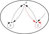
(a) Graph with all links	(b) Graph with only linear links

Figure 4: Graphs of the Rössler system. The root SCC (drawn as a thick circle) contains the three variables when the method considers all connections constant (a) and only variables $x$ and $y$ when nonlinearities are removed for building the graph (b).

Example 3.2 shows that this method, as acknowledged by the authors [Liu et al., 2013, p. 2464] is unable to indicate that measuring the $y$ variable from the Rössler system is preferrable to, say, measuring $z$. On the other hand, it was shown that this graphical approach underestimates the number of variables which must be necessarily measured [Haber et al, 2017, Letellier et al., 2018]. An improved version of this graphical approach was recently proposed [Letellier et al., 2018b], showing that nonlinear interactions should be removed for determining the root SCCs and that such graph only provides necessary but not sufficient conditions on the measurements for ensuring structural observability.

3.3 Ranking observable graphs

Lin’s method for structural observability in Sec. 3.1 was developed for linear systems for which the weights in the corresponding graph are constant. In determining non-accessible vertices only the presence or absence of edges is of concern. Therefore the method either classifies the graph as observable or not.

A more challenging situation is furnished by the pair $[A,\,\tilde{C}]$ with $A$ given in (33) and $\tilde{C}=[C_{1}~{}C_{2}]$, as follows. If $C_{2}\neq 0$ the pair stands a chance of being observable. Let us assume that it is observable, that is, the observability matrix (3) computed with the pair $[A,\tilde{C}]$ is full rank, hence the pair is structurally observable for the reasons given above. Structural observability will be lost only if $C_{2}=0$, and even for extremely small values of $C_{2}$, the pair will be structurally observable. Hence such type of observability will not distinguish among a whole range of pairs that can be either far or arbitrarily close to the condition $C_{2}=0$. A possible way out in this very simple example is to compute the condition number (12) for the observability matrices of $[A,\tilde{C}]$ for the different measuring situations that result in different $\tilde{C}$s. Ill-conditioned observability matrices will indicate unfavorable situations in terms of observability.

As for the method by Liu and coworkers for sensor set selection, the lack of discriminatory power pointed out in Example 3.2 is due to disregarding the differences in the type of edges, that is, the method treats full and dashed arrows alike. In order to rank the variables, features of the links should be taken into account, such as the weight of a link: small constant weights and variable weights will give rise to poorly observed regions in the graph.

It is interesting to notice that as it happened in the development of the theory of observability for dynamical systems, the first results classified graphs either as being observable or not. It seems that it would be desirable to see the development of procedures to rank graphs in terms of observability.

3.4 Symbolic observability of topologies

Provided that the symbolic Jacobian matrix ${\cal J}$ can be written for a graph then, in principle, symbolic observability coefficients can be computed. For relatively simple systems, to obtain ${\cal J}$ is straightforward, as the following example shows.

Example 3.3

We again consider the graph shown in Figure 1a. In a typical graph, there would be no distinction between full and dashed lines, as for the methods of Lin and of Liu and coworkers. Calling ${\cal J}^{0}$ a symbolic Jacobian matrix that does not  take into account the nonlinear connections, and ${\cal\tilde{J}}$ the standard symbolic Jacobian matrix [Bianco-Martinez et al., 2015], from system (10) we get

$${\cal J}^{0}=\left[\begin{array}[]{ccc}0&1&1\\ 1&1&0\\ 1&0&1\end{array}\right]\mbox{ and }{\cal\tilde{J}}=\left[\begin{array}[]{ccc}0&1&1\\ 1&1&0\\ \bar{1}&0&\bar{1}\end{array}\right].$$ (68)

Notice that ${\cal\tilde{J}}$ is the same as obtained in (28). Hence proceeding as in Example 2.5 the same symbolic observability coefficients obtained from the system equations are found using ${\cal\tilde{J}}$, that is, from the graph. If ${\cal J}^{0}$ is used instead, the result reached at is that any of the variables provide the same level of observability. This shows why the method by Liu and co-workers is unable to provide guidance of which sensor vertex to use within the root SCC which here (Figure 4a) contains the three variables. In the spirit of symbolic coefficients, the modified approach [Letellier et al., 2018b] does not take into account the nonlinear (dashed) edges (Figure 4b). $\triangle$

It is conceivable that for graphs of even moderate sizes, it might not be simple to build analytical observability matrix and even less to compute the determinant of the symbolic observability matrix. A software like Maple fails to compute the observability matrix of a 5D rational system [Letellier et al., 2018]. A similar difficulty is shared by all other methods that require the analysis of an observability matrix. Symbolic approaches are therefore an alternative to overcome this difficulty.

4 Types of Observability

The aim of this section is to recognize differences among types of observability in what concerns definitions and aims, as reviewed in sections 2 and 3. Also, interesting links between definitions will be pointed out and some extensions to networks will be proposed. The types of observability will be mentioned roughly in the same chronological order as they appear in the literature. The main results are summarized in Table 1.

4.1 Structural Observability

The adjective structural  was used by [Lin, 1974] to indicate cases in which controllability was robust against perturbations of unknown or uncertain parameters. Here we use structural  in a somewhat wider, but closely related, sense. All definitions of observability that classify a system in either observable or not will be included in the class of structural observability. The justification for this is that in such cases, observability only depends on the internal structure (presence and nature of coupling terms) of the system variables. Hence, in this sense, Kalman’s definition of observability and the nonlinear counterpart [Hermann and Krener, 1977] belong to this class although such are sometimes referred to as being definitions of complete  or full  observability. Other terms such as exact  and mathematical  controllability/observability have been used recently [Wang et al., 2017].

A slightly different aim has been pursued in [Liu et al., 2013] where a minimum set of sensor vertices is sought in order to render a graph observable. Nonetheless, the procedure either indicates situations in which the graph is or is not observable.

In spite of the varied terminology, there is one aspect common to all such procedures: the outcome is a classification of a system according to which it is either observable or not. In view of this, we classify all such procedures under the heading of structural observability. This is the case for the methods reviewed in sections 2.1, 3.1 and 3.2.

4.2 Dynamical Observability

In contrast to structural observability, we shall refer to dynamical observability  whenever there is a continuous quantification of our ability to estimate the state of a system from a finite set of data. In dynamical observability the key issue is to somehow quantify and distinguish those cases in which a system is close to becoming non observable from those in which it is far from that condition. This is done computing observability coefficients that measure how far from singularity, on average along a trajectory in state space, is the observability matrix, see discussion in sections 2.2 and 2.3. Therefore, an important aspect of this class of observability is that it only makes sense for systems that are  observable. Of course if a system is not observable, by definition the corresponding dynamical observability coefficient is zero. Hence dynamical observability helps us to rank observable  pairs $[\mbox{f},\,h_{i}(\mbox{\boldmath$x$})]$ for a given vector field f.

A similar situation in terms of controllability of linear complex networks has been reported, namely the situation in which a network is controllable however, in practice, control is very difficult to attain [Wang et al., 2017]. As argued by Cowan and coworkers: “more important than issues of structural controllability are the questions of whether a system is almost uncontrollable” [Cowan et al., 2012]. This is the typical situation in which a dynamical  rather than a structural  assessment of controllability or observability is called for. Dynamical observability was investigated in the context of three-node networks of Fitzhugh-Nagumo oscillators in [Whalen et al., 2015].

In assessing this type of observability, there are two challenges to be faced. First is how to quantify how far the system is, at a certain point, from the location in space where observability is lost, that is, where observability matrix becomes rank deficient. Second, how to average this result in order to have a single “global” indication of observability. In Sec. 2.2 these challenges were met by computing the condition number (13), and taking an average along a trajectory (14) which can be interpreted as a spatial average in state space. If the trajectory happens to be chaotic, then the average covers a wider region than in the case of a periodic trajectory.

Other ways of facing the first challenge would be to use the determinant of the observability matrix or its singular values. The fraction of time that the trajectory spends within a neighborhood of the singularity manifold has been used to assess dynamical observability [Frunzete et al., 2012].

The coefficients that quantify dynamical observability have only relative interpretation. For instance, in the case of the Rössler system for $(a,\,b,\,c)=(0.398,\,2,\,4)$ the coefficients are ordered thus $\delta_{y}>\delta_{x}>\delta_{z}$ therefore the $y$ variable conveys better observability of the system than variable $x$ which, in turn, is preferrable to $z$. Unfortunately, the coefficients for dynamical observability as defined by the condition number (13), are not comparable in general among different systems. This shortcoming is overcome by the coefficients for symbolic observability, as discussed in Sec. 2.5.

4.3 Symbolic Observability

Symbolic observability  shares some features of the previous types of observability and includes characteristics of its own. On the one hand, as with structural observability, symbolic observability does not depend on parameter values but only on the nonlinear couplings within the system variables. On the other hand, as with dynamical observability, symbolic observability is capable of ranking observable pairs.

Central to the definition of symbolic observability is the complexity of the singularities that appear in the symbolic observability matrix. Some advantages compared to the other definitions are the fact that it is more amenable to be computed for larger systems with more complicated dynamics [Bianco-Martinez et al., 2015], it provides “normalized” results in the range $[0;1]$ that permit comparing different systems in terms of observability. Related to this, it has been argued that systems with a symbolic observability coefficient greater than 0.75 have good overal observability properties [Sendiña-Nadal et al., 2016].

These symbolic coefficients are very promising for assessing the observability of systems and networks that are larger than the ones analyzed with the dynamical observability coefficients [Letellier et al., 2018].

5 Observability of Dynamical Networks: Numerical Results

A dynamical network is a set of dynamical systems – oscillators – interconnected according to the network topology which is described by the corresponding adjacency matrix. The aim is to discuss, in the context of a simple example where the node dynamics is linear, some of the aspects seen so far.

Here we will consider a network whose topology is described by the adjacency matrix

$$A_{\rm adj}=\left[\begin{array}[]{ccc}0&a_{12}&0\\ a_{21}&0&a_{23}\\ 0&a_{32}&0\end{array}\right],$$ (72)

and for which at each node there is a three-dimensional dynamical system

$$S_{i}:\left\{\begin{array}[]{l}\dot{x}_{i}=-y_{i}\\ \dot{y}_{i}=x_{i}\\ \dot{z}_{i}=\alpha x_{i}-z_{i}\,.\end{array}\right.$$ (73)

Nodes are coupled via one of their variables ($x_{i}$, $y_{i}$ or $z_{i}$). In this network, the term $a_{32}$ may vanish, for instance due to a nonlinearity. In what follows, we adopt the convention that the element $a_{ij}$ of the adjacency matrix $A_{\rm adj}$ corresponds to an edge from vertex $j$ to vertex $i$ [Newman, 2010, Sec. 6.2]. If the other convention were adopted, we would have to use $A_{\rm adj}^{\scriptscriptstyle\rm T}$ in place of matrix $A$ or the Jacobian matrix.

Consequently, following Newman’s convention, controllability can be investigated by considering the pair $[A_{\rm adj},\,\mbox{\boldmath$b$}]$ where the input vector is $\mbox{\boldmath$b$}=[0~{}0~{}1]^{\scriptscriptstyle\rm T}$, indicating the situation in which only system $S_{3}$ receives the driving signal (Figure 5). As long as $a_{32}\neq 0$ the network is structurally topologically  controllable since each node can be reached from vertex $v_{3}$ (Figure 5a). The topological  observability of the network can be analyzed using the dual pair $[A_{\rm adj}^{\scriptscriptstyle\rm T},\mbox{\boldmath$c$}]$ where the output vector is $\mbox{\boldmath$c$}=[0~{}0~{}1]^{\scriptscriptstyle\rm T}$, indicating the situation in which only one or more variables from system $S_{3}$ can be measured (Figure 5b). As long as $a_{32}\neq 0$ the network is structurally topologically observable. A similar conclusion can be drawn directly from the graph shown Figure 5a but reversing the edge from vertex $v_{3}$: as long as $a_{32}\neq 0$, information from nodes $S_{1}$ and $S_{2}$ can flow up to the measurements (vertex $v_{3}$) and, consequently, the network is structurally topologically observable.

(a) Graph of the pair $[A_{\rm adj},\mbox{b}_{3}]$	(b) Graph of the pair $[A_{\rm adj}^{\scriptscriptstyle\rm T},\mbox{c}_{3}]$

Figure 5: (a) Graph of the network whose topology is described by the adjacency matrix (72) with a single driving node $S_{3}$, and (b) the corresponding dual graph. If $a_{32}$ vanishes in (b), nodes $S_{1}$ and $S_{2}$ become non-accessible and the dual network is no longer structurally controllable, meaning that the pair $[A_{\rm adj},\mbox{c}_{3}^{\scriptscriptstyle\rm T}]$ is no longer structurally observable from $S_{3}$ if $a_{32}$ vanishes.

Using symbolic observability and treating the adjacency matrix $A_{\rm adj}$ as a Jacobian matrix, it is readily found that the network in Figure 5a is not topologically observable from $S_{2}$ ($\eta_{2}^{3}=0$), it is fully topologically observable from $S_{1}$ ($\eta_{1}^{3}=1$) and is poorly topologically observable from $S_{3}$ ($\eta_{3}^{3}=0.56$). The lack of observability from $S_{2}$, which can be readily confirmed from linear system theory, is not obvious, as this node receives information from the other two nodes. This result seems to be in line with the discussion presented in [Leitold et al., 2017].

Nevertheless, when considering the observability of a dynamical network as shown in Figure 5a with nodal dynamics (e.g. as given in Eq. 73), it must be realized that the topological observability only provides a partial answer. In order to ensure structural observability of the full network from, say, $v_{3}$, not only every node of the dual pair $[A_{\rm adj}^{\scriptscriptstyle\rm T},[0~{}0~{}1]^{\scriptscriptstyle\rm T}]$ (Figure 5b) that must be accessible by acting on $v_{3}$ but also every vertex of the graph describing the full network as shown in Figure 6a. Consequently the result strongly depends on the observability conveyed by the variable used in measuring the sensor node and  the one used for coupling the nodes.

Since (73) is linear, it is straightforward to verify that the pair $[D\mbox{f}_{3},\mbox{\boldmath$c$}_{3}^{\scriptscriptstyle\rm T}]$ is structurally observable only if the measured variable is $z_{3}$ (that is, $\mbox{\boldmath$c$}_{3}^{\scriptscriptstyle\rm T}=[0~{}0~{}1]$) and $\alpha\neq 0$. The pair $[D\mbox{f}_{3},\,\mbox{\boldmath$c$}_{3}^{\scriptscriptstyle\rm T}]$ is not structurally observable when $\mbox{\boldmath$c$}_{3}^{\scriptscriptstyle\rm T}=[1~{}0~{}0]$ or $\mbox{\boldmath$c$}_{3}^{\scriptscriptstyle\rm T}=[0~{}1~{}0]$. Therefore, although the network is structurally topologically  observable from $S_{3}$ ($a_{32}\neq 0$), it is only structurally observable if variable $z_{3}$ is recorded at $S_{3}$. In addition, if $\alpha=0$, the network is not  structurally observable even for $a_{32}\neq 0$. Indeed as shown by the unfolded graph of the network in Figure 6a, the node dynamics, $S_{3}$, is structurally observable when variable $z_{3}$ is measured ($\eta_{z_{3}^{3}}=1$, Det $\frac{\partial\Phi}{\partial\mbox{x}}=-\alpha^{2}$ where $\Phi\,:(x_{3},y_{3},z_{3})\mapsto(z_{3},\dot{z}_{3},\ddot{z}_{3})$) and is not observable when $x_{3}$ or $y_{3}$ ($\eta_{x_{3}^{3}}=\eta_{y_{3}^{3}}=0$) are measured.

When the nodes of the full network are coupled by variable $z$ there is a directed path from every vertex to vertex $z_{3}$ if $\alpha\neq 0$. To see that the network observability also depends on the coupling consider when coupling is accomplished via variable $x$ (or similarly via variable $y$). The unfolded graph drawn in Figure 6b shows that the resulting network will only be structurally observable if $z_{1}$, $z_{2}$ and $z_{3}$ are simultaneously recorded, even for $\alpha\neq 0$ and $a_{32}\neq 0$.

(a) Coupled via variable $z$		(b) Coupled via variable $x$

Figure 6: Graph of the full network in Figure 5a. The details of the node dynamics are included. If $z_{3}$ is measured, and $\alpha=0$ the network is not structurally observable regardless of the value of $a_{32}$.

The previous examples helps to understand why Gates and Rocha have argued that to represent nodes as variables lacks intrinsic dynamics and that there is often a discrepancy between results related to controllability that take into account only the graph structure [Gates and Rocha, 2016].

To summarize, in investigating the observability of a dynamical network, not only the topology but also the local dynamics of sensor nodes and the coupling variables must be taken into account. For the sake of clarity, when a full network is investigated, these three ingredients must be considered: i) nodes connected according to an adjacency matrix (a graph), ii) the coupling and iii) the node dynamics.

Structural topological observability of the full network (Figure 6) whose topology is described by $A_{\rm adj}$ (Figure 5a) will only detect when observability is completely lost and is insensitive to a gradual reduction in observability due to the decrease of $a_{32}$ or in $\alpha$. Here the simple procedure discussed in [Aguirre, 1995] will suffice to provide an indication of the gradual reduction in topological observability using (12) applied to the adjacency matrix $A_{\rm adj}$ from Eq. (72) if the dynamics are linear and, using (14) if nonlinear. Dynamical observability of the toplogy of the network, disregarding the node dynamics, is shown in Figure 7a whereas the dynamical observability of uncoupled node dynamics is shown in Figure 7b. These plots resemble the overall shape of the plots presented in Ref. [Whalen et al., 2015, see their Fig. 5] where for small coupling the observability coefficient is very low; it increases with the coupling up to a maximum, and then gradually falls as the coupling is further increased.

For the full network in Figure 6a, that is, when three systems (73) are coupled by their variable $z$ according to the adjacency matrix (72) and when variable $z_{3}$ is measured the observability coefficients are shown in Figure 7c. Slices of this plot retains some features of the two previous ones. However, when the nodes are coupled through variable $x$ accordind to the same  adjacency matrix, the observability is practically lost as illustrated in Figure 7d, where the values in the plot are all close to zero within machine accuracy. This shows that a joint anlysis is required, that is, not only node dynamics and how the nodes are connected must be used, but also the coupling variables must be taken into account.

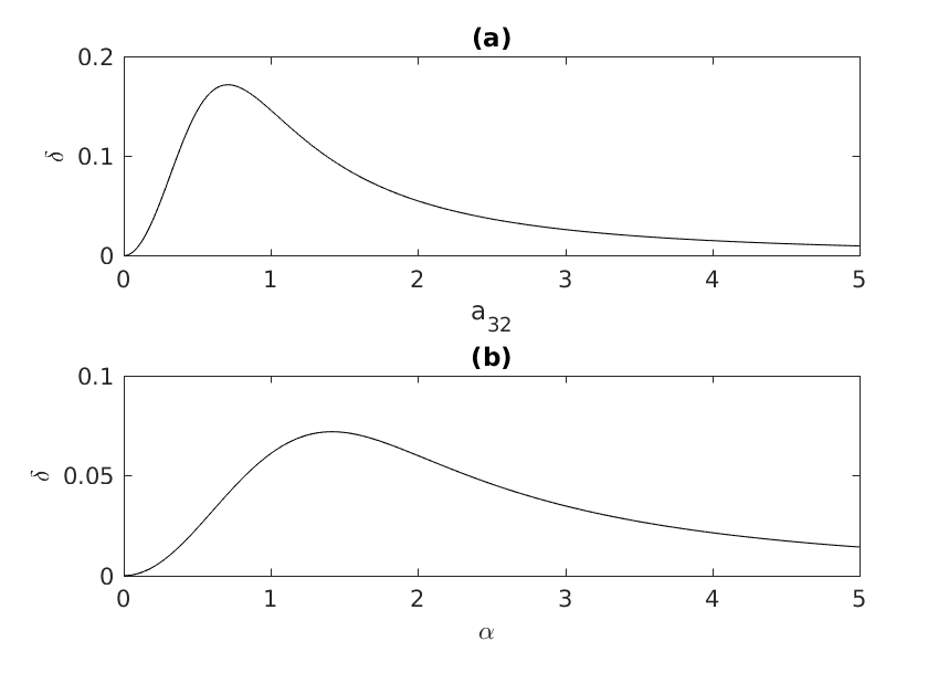
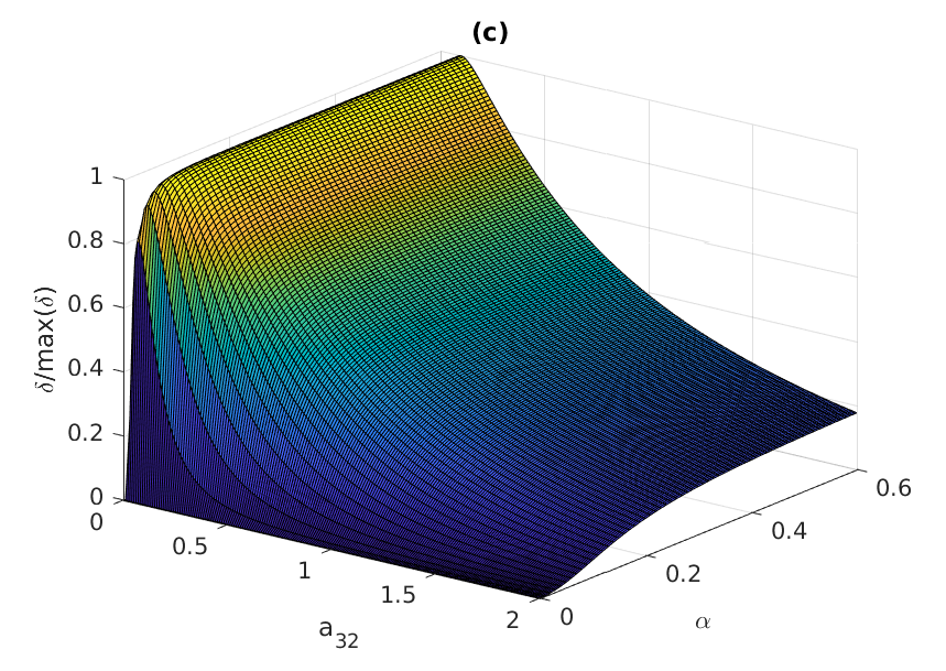
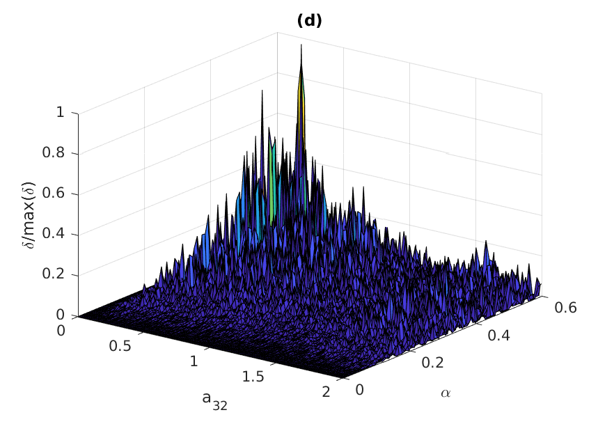
Figure 7: Observability coefficient (12) computed (a) for the network topology shown in Figure 5a, (b) for the node dynamics in (73). Mathematically, the node dynamics becomes not structurally observable from $z_{3}$ only for $\alpha=0$, and the network becomes structurally not topologically observable from the sensor node $S_{3}$ only for $a_{32}=0$. Normalized observability coefficients (c) for the full network coupled using $z$ (Fig. 6a), and (d) coupled using $x$ (Fig. 6b).

This result only provides a partial answer. A more acurate analysis can be performed using Det$\frac{\partial\Phi_{s}}{\partial\mbox{x}}$. First we set $a_{12}=a_{21}=0$ to treat a two node network $\{S_{2},S_{3}\}$ with measurements in node $S_{3}$, either $x_{3}$, $y_{3}$ or $z_{3}$. We were able to get a full rank $6\times 6$ observability matrix with $\Phi_{x_{3}y_{3}z_{3}^{4}}$, $\Phi_{x_{3}^{2}z_{3}^{4}}$ or $\Phi_{y_{3}^{2}z_{3}^{4}}$ for which the determinants were equal to $\pm a_{32}^{3}\alpha^{2}$. The full network becomes structurally non observable when $\alpha_{32}$ or $\alpha$ is equal to zero as already found. Therefore, the network is observable from $S_{3}$ if we measure $z_{3}$ plus, at least, another variable from that node.

This simple example shows that investigating a dynamical network by only analyzing the network observability from the adjacency matrix can lead to wrong results because the topological observability is only correct in the extreme case where the nodes are not only coupled but also observed by the variable providing the best observability. If the network is structurally topologically observable, then the network observability depends on the variable with which node dynamics are coupled and observed. Consequently, topological observability must be at least associated with an analysis of the observability of the node dynamics (the isolated system acting at each node) and it must be checked whether the coupling conveys the information up to the measured variable.

6 Conclusions

Two decades have past since it was argued that a procedure borrowed from the theory of observability of linear systems could be adapted to explain why global modeling algorithms performed differently using different recorded variables [Letellier et al., 1998]. This paper has aimed at providing a general view of how some concepts related to observability have developed in the realm of nonlinear dynamics and to point out some important differences among the approaches. In order to make distinctions clearer, some different types of observability measures were proposed. Also, the use of the discussed techniques in the field of dynamical networks has been discussed briefly. An overview is provided in Table 1.

An important point to realize is that whereas the definition of observability aims to classify a system as being observable or not, a more interesting challenge is to be able to rank variables of observable systems  in terms of the potential performance each would have in certain practical situations. The first problem has been connected to structural observability, whereas the second one to dynamical and symbolic observability. These concepts can be readily applied to dynamical systems or to dynamical networks and their three levels of description, namely: node dynamics, topology and the full network.

However, as for the observability of dynamical networks, some limitations of graph-based procedures have been pointed out. It has been argued that the observability of a dynamical network depends on three ingredients: i) the topology described by the adjacency matrix – called topological observability in this paper–; ii) the variable used for coupling nodes and iii) the observability of node dynamics. It was shown that the topological observability of a network — only based on the adjacency matrix — can provide spurious assessment of the observability of the full network in certain cases. In the case of dynamical networks, which are composed of oscillators at the nodes interconnected according to a topology, topological observability does not seem adequate to accurately characterize a network dynamics.

Table 1: Summary of types of observability and systems. Yes/No refers to practical applicability of numerical procedures discussed in the paper. The “Node dynamics” corresponds to low-dimensional dynamical systems interconnected according to a “Topology” to form a dynamical “Network”.

Type of	Task	Node dynamics	Topology	Networks
Observability		Sec. 2	Sec. 3	Sec. 5
Structural	observable vs.	Yes	Yes	Yes
Sec. 4.1	nonobservable	Sec. 2.1	Sec. 3.1–3.2
	classification
Symbolic	Ranking variables	Yes	Yes	Yes
Sec. 4.3		Sec. 2.5	Sec. 3.4
Dynamical	Ranking variables	Yes	Only for small	No
Sec. 4.2		Sec. 2.2–2.4	dimension Sec. 3.3

References

- [Aguirre, 1995] Aguirre, L. A. (1995). Controllability and observability of linear systems: some noninvariant aspects. IEEE Transactions on Education, 38:33–39.
- [Aguirre and Letellier, 2005] Aguirre, L. A. and Letellier, C. (2005). Observability of multivariable differential embeddings. J. Phys. A: Math. Gen., 38:6311–6326.
- [Aguirre and Letellier, 2011] Aguirre, L. A. and Letellier, C. (2011). Investigating observability properties from data in nonlinear dynamics. Physical Review E, 83(066209).
- [Bianco-Martinez et al., 2015] Bianco-Martinez, E., Baptista, M. S., and Letellier, C. (2015). Symbolic computations of nonlinear observability. Physical Review E, 91(062912).
- [Casdagli et al., 1991] Casdagli, M., Eubank, S., Farmer, J. D., and Gibson, J. (1991). State space reconstruction in the presence of noise. Physica D, 51:52–98.
- [Chang and Shachter, 1992] Chang, B. Y. and Shachter, R. D. (1992). Structural controllability and observability in influence diagrams. In Proceedings of the 8th Conference on Uncertainty in Artificial Intelligence, Standford University, July, pages 25–32.
- [Chen, 1999] Chen, C. T. (1999). Linear System Theory and Design. Oxford University Press, Oxford.
- [Cowan et al., 2012] Cowan, N. J., Chastain, E. J., Vilhena, D. A., Freudenberg, J. S., and Bergstrom, C. T. (2012). Nodal dynamics, not degree distributions, determine the structural controllability of complex networks. PLoS ONE, 7(6):e38398.
- [Friedland, 1975] Friedland, B. (1975). Controllability index based on conditioning number. Journal of Dynamic Systems, Measurement, and Control, 97(4):444–445.
- [Frunzete et al., 2012] Frunzete, M., Barbot, J. P., and Letellier, C. (2012). Influence of the singular manifold of nonobservable states in reconstructing chaotic attractors. Phys. Rev. E, 86(2):026205.
- [Gates and Rocha, 2016] Gates, A. J. and Rocha, L. M. (2016). Control of complex networks requires both structure and dynamics. Sci. Rep., 6(24456).
- [Haber et al, 2017] Haber, A. and Molnar, F. and Motter, A. E. (2017), State observation and sensor selection for nonlinear networks. IEEE Transactions on Control of Network Systems , DOI: 10.1109/TCNS.2017.2728201.
- [Hermann and Krener, 1977] Hermann, R. and Krener, A. J. (1977). Nonlinear controllability and observability. IEEE Trans. Automat. Contr., 22(5):728–740.
- [Kalman, 1960] Kalman, R. E. (1960). On the general theory of control systems. In Proc. First IFAC Congress Automatic Control, pages 481–492, London. Butterworths.
- [Leitold et al., 2017] Leitold, D., Vathy-Fogarassy, A., and Abonyi, J. (2017). Controllability and observability in complex networks – the effect of connection types. Scientific Reports, 7(151).
- [Letellier, 2006] Letellier, C. (2006). The Shannon entropy: recurrence plots versus symbolic dynamics. Phys. Rev. Lett., 96:254102.
- [Letellier and Aguirre, 2002] Letellier, C. and Aguirre, L. A. (2002). Investigating nonlinear dynamics from time series: the influence of symmetries and the choice of observables. Chaos, 12(3):549–558.
- [Letellier and Aguirre, 2005] Letellier, C. and Aguirre, L. A. (2005). A graphical interpretation of observability in terms of feedback circuits. Physical Review E, 72(056202).
- [Letellier and Aguirre, 2009] Letellier, C. and Aguirre, L. A. (2009). Symbolic observability coefficients for univariate and multivariate analysis. Physical Review E, 79(066210).
- [Letellier et al., 2005] Letellier, C., Aguirre, L. A., and Maquet, J. (2005). Relation between observability and differential embeddings for nonlinear dynamics. Physical Review E, 71(066213).
- [Letellier et al., 1998] Letellier, C., Maquet, J., Le Sceller, L., Gouesbet, G., and Aguirre, L. A. (1998). On the non-equivalence of observables in phase-space reconstructions from recorded time series. J. of Phys. A, 31:7913–7927.
- [Letellier et al., 2018] Letellier, C., Sendiña Nadal, I., Bianco-Martinez, E., and Baptista, M. S. (2018). A symbolic network-based nonlinear theory for dynamical systems observability. Scientific Report, 8, 3785.
- [Letellier et al., 2018b] Letellier, C., Sendiña Nadal, I., and Aguirre, L. A. (2018). A nonlinear graph-based theory for dynamical network observability. arXiv:1803.00851v2 [nlin.CD]
- [Lin, 1974] Lin, C.-T. (1974). Structural controllability. IEEE Transactions on Automatic Control, 19(3):201–208.
- [Liu et al., 2013] Liu, Y. Y., Slotine, J. J., and Barabási, A. L. (2013). Observability of complex systems. Proceedings of the National Academy of Sciences of the United States of America, 110(7):2460–2465.
- [Newman, 2010] Newman, M. E. J. (2010). Networks: An Introduction. Oxford University Press, Oxford.
- [Rössler, 1976] Rössler, O. E. (1976). An equation for continuous chaos. Phys. Lett., 57A(5):397–398.
- [Schiff, 2012] Schiff, S. J. (2012). Neural Control Engineering. The MIT Press, Cambridge, Massachusetts.
- [Sedigh-Sarvestani et al., 2012] Sedigh-Sarvestani, M., Schiff, S. J., and Gluckman, B. J. (2012). Reconstructing mammalian sleep dynamics with data assimilation. PLoS Comput Biol, 8(11):e1002788.
- [Sendiña-Nadal et al., 2016] Sendiña-Nadal, I., Boccaletti, S., and Letellier, C. (2016). Observability coefficients for predicting the class of synchronizability from the algebraic structure of the local oscillators. Phys. Rev. E, 94 (042205).
- [Sendiña-Nadal et al., 2018] Sendiña-Nadal, I., Aguirre, L. A., and Letellier, C. (2018). Selecting the variables to measure in networks and the related structural, symbolic and topological observabilities. In preparation.
- [Su et al., 2017] Su, F., Wang, J., Li, H., Deng, B., Yu, H., and Liu, C. (2017). Analysis and application of neuronal network controllability and observability. Chaos, 27(023103).
- [Takens, 1981] Takens, F. (1981), Detecting strange attractors in turbulence. Lecture Notes in Mathematics, 898: 366-381.
- [Wang et al., 2017] Wang, L.-Z., Chen, Y.-Z., Wang, W.-X., and Lai, Y.-C. (2017). Physical controllability of complex networks. Scientific Reports, 7: 40198.
- [Whalen et al., 2015] Whalen, A. J., Brennan, S. N., Sauer, T. D., and Schiff, S. J. (2015). Observability and controllability of nonlinear networks: The role of symmetry. Phys. Rev. X, 5: 011005.