Emotion Representation Mapping for Automatic Lexicon Construction (Mostly) Performs on Human Level

Abstract

Emotion Representation Mapping (ERM) has the goal to convert existing emotion ratings from one representation format into another one, e.g., mapping Valence-Arousal-Dominance annotations for words or sentences into Ekman’s Basic Emotions and vice versa. ERM can thus not only be considered as an alternative to Word Emotion Induction (WEI) techniques for automatic emotion lexicon construction but may also help mitigate problems that come from the proliferation of emotion representation formats in recent years. We propose a new neural network approach to ERM that not only outperforms the previous state-of-the-art. Equally important, we present a refined evaluation methodology and gather strong evidence that our model yields results which are (almost) as reliable as human annotations, even in cross-lingual settings. Based on these results we generate new emotion ratings for 13 typologically diverse languages and claim that they have near-gold quality, at least.

1 Introduction

From its inception, researchers in the field of sentiment analysis aimed at predicting the affective state that is typically associated with a given word based on a list of linguistic features, a problem referred to as word emotion induction (WEI) [Hatzivassiloglou and McKeown, 1997, Turney and Littman, 2003]. Early research activities have focused on semantic polarity (the positiveness or negativeness of a feeling) for quite a long time. But more recently this focus on binary representations has been replaced by more expressive emotion representation formats such as Basic Emotions or Valence-Arousal-Dominance. In the meantime, WEI has become an active area of research, regularly featured in shared tasks [Rosenthal et al., 2015, Yu et al., 2016b]. Based on these achievements, WEI techniques have become a natural methodological choice for the automatic construction of emotion lexicons [Köper and Schulte im Walde, 2016, Shaikh et al., 2016].

Yet, only very recently, a radically different approach to automatic emotion lexicon construction has been proposed. Instead of relying on linguistic features (such as similarity with seed words or word embeddings), the goal of emotion representation mapping (ERM) is to derive new emotional word ratings in one format based on known ratings of the same words in another format [Buechel and Hahn, 2017a]. For example, ERM could use empirically gathered ratings for Basic Emotions and convert them into a Valence-Arousal-Dominance representation scheme, with greater precision than currently achievable by WEI algorithms. As a much appreciated side effect, one of the promises of ERM is to make otherwise incompatible resources (lexicons or annotated corpora, as well as tools) compatible, and incomparable systems comparable. Thus, this approach has the potential to mitigate some of the negative effects that arise from not having a community-wide standard for emotion annotation and representation [Calvo and Mac Kim, 2013, Buechel and Hahn, 2018a].

We here want to contribute to this endeavor by providing a large-scale evaluation of previously proposed ERM approaches for four typologically diverse languages and report evidence that ERM clearly outperforms current state-of-the-art WEI algorithms. Furthermore, we present our own deep learning model which performs even better against all competitors. Most importantly, however, we propose a new methodology for comparing the reliability of ERM against human annotation reliability, a major shortcoming of previous work. As a result, we find that our proposed model performs competitive to a reasonably large group of human raters, even in cross-lingual settings. Based on this evidence, we automatically construct emotion lexicons for 13 languages and claim that they have (near) gold quality. These lexicons as well as our experimental code base and results are publically available.

2 Related Work

Psychological Models of Emotion.

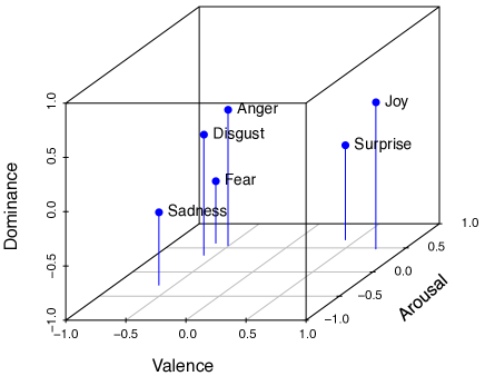
Figure 1: Affective space spanned by the Valence-Arousal-Dominance (VAD) model, together with the position of six Basic Emotions. Adapted from ?).

Models of emotion typically fall into two main groups, namely discrete (or categorical) and dimensional ones [Stevenson et al., 2007, Calvo and Mac Kim, 2013]. Discrete models are built around particular sets of emotional categories deemed fundamental and universal. ?), for instance, identifies six Basic Emotions (Joy, Anger, Sadness, Fear, Disgust and Surprise). In contrast, dimensional models consider emotions to be composed out of several influencing factors (mainly two or three). These are often referred to as Valence (corresponding to the concept of polarity), Arousal (a calm–excited scale), and Dominance (perceived degree of control over a (social) situation)—the VAD model. The last dimension, Dominance, is quite often omitted, thus constituting the VA model. For convenience, both will be jointly referred to as VA(D). An illustration of VAD and its relationship to Basic Emotions is given in Figure 1.

Lexical Data Sets.

In contradistinction to NLP where many different representation formats for emotions are being used, lexical resources originating from psychology labs almost exclusively subscribe either to VA(D) or Basic Emotions models (typically omitting Surprise; the BE5 format). Over the years, a considerable number of resources built on these premises have emerged from psychological research for various languages. In more detail, these lexical ratings have been gathered via questionnaire studies by collecting individual ratings from a large number of subjects for each lexical item under consideration (typically between 20 to 30 individual ratings per item). These individual assessments are then averaged to yield aggregated scores on which we base our experiments. The emotion values we deal with must thus be understood as an average emotional reaction when presenting a lexical stimulus to a group of human judges.

Abbrev.	VA(D)	BE5	Dom?	Overlap
en_1	?)	?)	✓	1,028
en_2	?)	?)	✓	1,027
es_1	?)	?)	✓	1,012
es_2	?)	?)	✓	875
es_3	?)	?)	✗	10,491
de_1	?)	?)	✗	1,958
pl_1	?)	?)	✗	2,902
pl_2	?)	?)	✓	1,272

Table 1: Data sets used in our experiments; with abbreviation (including language code according to ISO 639-1), the bibliographic sources of the VA(D) and BE5 ratings, information on whether Dominance is included and the number of overlapping entries.

In this paper, we restrict ourselves to the VA(D) and BE5 format. Following the conventions of the emotion lexicons used in our experiments (Table 1), each VA(D) dimension receives a value from the interval $[1,9]$ where ‘1’ means “most negative/calm/submissive”, ‘9’ means “most positive/excited/dominant” and ‘5’ means “neutral”. Conversely, values for BE5 categories range in the interval $[1,5]$ where ‘1’ means “absence” and ‘5’ means “most extreme” expression of the respective emotion. Consequently, the VA(D) and BE5 formats are conceptually different from one another insofar as VA(D) dimensions are bi-polar, whereas BE5 categories are uni-polar.

Word Emotion Induction.

Automatically constructing such word-level emotion data sets has been a focus of NLP-based sentiment analysis studies from the beginning. In fact, the problem to automatically predict polarity or emotion scores for a given word based on some linguistic features—often referred to as Word Emotion Induction (WEI)—is already dealt with in the seminal work of ?). At first, the features taken into account were typically derived from co-occurrence or terminology-based similarity with a small set of seed word with known emotional scores [Turney and Littman, 2003, Esuli and Sebastiani, 2005]. Nowadays, these features are almost completely replaced by word embeddings, i.e., dense, low-dimensional vector representations of words that are trained on large volumes of raw text in an unsupervised manner. Word2Vec [Mikolov et al., 2013], GloVe [Pennington et al., 2014] and FastText [Bojanowski et al., 2017] are among today’s most popular algorithms for generating embeddings.

WEI algorithms constitute a natural baseline for ERM because, first, they produce the same output (emotion ratings for words according to some emotion representation format), yet their predictions are based on expressively weaker features (word embeddings instead of emotion ratings for the same word but in another format), thus constituting a harder task. Second, they form the currently prevailing paradigm for the automatic construction of emotion lexicons [Köper and Schulte im Walde, 2016, Shaikh et al., 2016], a problem for which ERM offers a promising alternative.

Emotion Representation Mapping.

Word	V	A	D	J	A	S	F	D
sunshine	8.1	5.3	5.4	4.3	1.2	1.3	1.3	1.2
terrorism	1.6	7.4	2.7	1.1	3.0	3.4	4.1	2.5
orgasm	8.0	7.2	5.8	4.3	1.3	1.3	1.4	1.2

Table 2: Three lexical items and their emotion values in VAD (second column group) and BE5 (third column group) format. VAD scores are taken from ?), BE5 scores were automatically derived (see Section 4.4).

In contrast to WEI, ERM is based on the condition that the pairs of data sets in Table 1 are complementary in the sense that, when combining these lexicons, a subset of their entries are then encoded in both emotion formats, i.e., VA(D) and BE5. This condition is illustrated for three lexical items in Table 2.

Although such complementary data sets have been available for quite some time, ERM has only recently been introduced to NLP by ?) in order to compare a newly proposed VAD-based prediction system against previously established results on Basic Emotion gold standards. In a follow-up study, ?) devised EmoBank, a VAD-annotated corpus which, in part, also bears BE5 ratings on the sentence level. They found that both kinds of annotation were highly predictive for each other using a $k$-Nearest-Neighbor approach. In later studies, they examined the potential of ERM as a substitute for manual annotation of lexical items, also in cross-lingual settings [Buechel and Hahn, 2017a, Buechel and Hahn, 2018a]. Although their evaluation was limited in expressiveness, they already found evidence that ERM may be comparable to human performance in terms of the quality of the resulting ratings.

Similar work has, to the best of our knowledge, only been done in the psychology domain. However, related work from this area does not target the goal of predictive modeling [Stevenson et al., 2007, Pinheiro et al., 2017]. In both contributions, linear regression models were fitted to predict VAD dimensions given BE5 categories and vice versa. Yet, this was mainly done to inspect the respective slope-coefficients as an indicator of the relationship of dimensions and categories. Thus, the overall goodness of the fit was not in the center of interest and was not even reported by ?).

3 Methods

Let $L\coloneqq\{w_{1},w_{2},...,w_{n}\}$ be a set of words. Let $s$,$t$ denote two distinct emotion representation formats such that both $emo^{s}(w_{i})\in\mathbb{R}^{|s|}$ and $emo^{t}(w_{i})\in\mathbb{R}^{|t|}$ describe the emotion vector associated with $w_{i}$ relative to $s$ and $t$, respectively, where $|s|$, $|t|$ denote the number of variables which each format employs (e.g., 3 for VAD and 5 for BE5). The task we address in this paper is to predict the target emotion ratings $T\coloneqq\{emo^{t}(w_{i})|\;w_{i}\in L\}$ given the set $L$ and the corresponding source emotion ratings $S\coloneqq\{emo^{s}(w_{i})|\;w_{i}\in L\}$. Performance will be measured as Pearson correlation $r$ between the predicted values and human gold ratings (one $r$-value per element of the target representation). In general, the Pearson correlation between two data series $X:=x_{1},x_{2},...,x_{n}$ and $Y:=y_{1},y_{2},...,y_{n}$ takes values between $+1$ (perfect positive correlation) and $-1$ (perfect negative correlation) and is computed as

$$r_{xy}\coloneqq\frac{\sum_{i=1}^{n}(x_{i}-\bar{x})(y_{i}-\bar{y})}{\sqrt{\sum_{i=1}^{n}(x_{i}-\bar{x})^{2}}\;\sqrt{\sum_{i=1}^{n}(y_{i}-\bar{y})^{2}}}$$ (1)

where $\bar{x}$ and $\bar{y}$ denote the mean values for $X$ and $Y$, respectively.

3.1 Reference Methods

The first method against which we will compare our proposed model is linear regression (LR) as used by ?) in their early study. LR predicts an emotion value in the target representation $t$ as the affine transformation

$$emo_{\text{LR}}^{t}(w_{i})\coloneqq W\;emo^{s}(w_{i})+b$$ (2)

where $W$ is a $|t|\times|s|$ matrix and $b$ is a $|t|\times 1$ vector. The model parameters are fitted using ordinary least squares. In contrast, ?) proposed the use of k-Nearest-Neighbor Regression (KNN) for ERM. This simple supervised approach predicts the target value as

$$emo^{t}_{\text{KNN}}(w_{i})\coloneqq\frac{1}{k}\sum_{{w_{i}}^{\prime}\in\text{NEAREST}(w_{i},k,S)}emo^{t}({w_{i}}^{\prime})$$ (3)

where NEAREST yields the $k$ nearest neighbors of $w_{i}$ in the training set (determined by the Euclidean distance between the source representations of two words). The $k$ parameter was fixed to $20$ based on a pilot study. We used the scikit-learn.org implementation for both LR and KNN.

3.2 Proposed Model: A Multi-Task Feed-Forward Neural Network for ERM

Despite the fact that the above set-ups already perform quite well for ERM (see Section 4), both LR and KNN are rather basic types of models lacking deeper sophistication. As a consequence, we here propose the use of Feed-Forward Neural Networks (FFNNs) for ERM which have been shown to be capable of approximating arbitrary functions, in theory at least [Hornik, 1991]. In general, an FFNN consists of an input layer with activation $a^{(0)}\coloneqq emo^{s}(w_{i})\in\mathbb{R}^{|s|}$ followed by multiple hidden layers with activation $a^{(l+1)}\coloneqq\sigma(W^{(l+1)}a^{(l)}+b^{(l+1)})$ where $W^{(l+1)}$ and $b^{(l+1)}$ are the weights and biases for layer $l+1$ and $\sigma$ is a nonlinear activation function. Since the emotion formats under scrutiny capture affective states as real-valued vectors, the activation on the output layer $a^{out}$ (where $out$ is the number of non-input layers in the network) is computed as the affine transformation

$$emo^{t}_{\text{FFNN}}(w_{i})\coloneqq a^{(out)}\coloneqq W^{(out)}a^{(out-1)}+b^{(out)}$$ (4)

Consequently, our model differs from the other approaches presented in this section by sharing model parameters (weights and biases of the hidden layers) across the different dimensions/categories of the target format with only the last layer having parameters which are uniquely associated to one of the outputs (see Equation 4). This can be considered as a mild form of multi-task learning [Caruana, 1997], a machine learning technique which has been shown to strongly decrease the risk of overfitting [Baxter, 1997] and also speeds up computation by greatly decreasing the number of tunable parameters compared to training individual layers for each affective dimension/category.

The remaining specifications of our model are as follows. We train two-hidden layer FFNNs (both with 128 units), ReLU activation, $.2$ dropout on the hidden layers (none on the input layer) and Mean-Squared-Error loss. Each model was trained for $10,000$ iterations (well beyond convergence, independently of the size of the training set) using the Adam optimizer [Kingma and Ba, 2015]. Keras.io was used for implementation.

3.3 Baseline: Word Emotion Induction

As a natural baseline for ERM, we will use a recent state-of-the-art method for word emotion induction (WEI) by ?). They propose Feed-Forward Neural Networks (similar to our proposed model for ERM) in combination with a boosting algorithm. The authors used FFNNs with a single hidden layer of $100$ units and ReLU activation. The boosting algorithm AdaBoost.R2 [Drucker, 1997] was used to train the ensemble (one per target variable). We implemented this approach with scikit-learn using exactly the same settings as in the original publication. As for the word embeddings this method needs as input, we used the pre-trained FastText embeddings that Facebook Research makes available for a wide range of languages trained on the respective Wikipedias. This way, we hope to achieve a particularly high level of comparability across languages because, for each of them, embeddings are trained on data from the same domain and of a similar order of magnitude.

3.4 Comparison to Human Reliability

Since common metrics for Inter-Annotator Agreement (IAA), such as Cohen’s Kappa, are not applicable for real-valued emotion scores [Carletta, 1996], we will now discuss how to compare our own results against human assessments in order to put their reliability on a safe ground.

One possible point of comparison that has been used in previous work [Buechel and Hahn, 2017a, Buechel and Hahn, 2018a] is inter-study reliability (ISR), i.e., the correlation between the ratings of common words in different data sets. However, this procedure comes with a number of downsides. First, the number of pairs of data sets with substantially overlapping entries is rather small since researchers focus mainly on acquiring ratings for novel words instead of gathering annotations anew for ones already covered. Thus, employing ISR comparison with human performance is only possible on few data sets. In particular, we are not aware of any pair of data sets with significantly overlapping BE5 ratings. Second, ISR is sensitive to differences in acquisition methodologies (e.g., alternative sets of instructions or rating scales) and may thus vary substantially between different pairs of data sets.

As an alternative, these shortcomings lead us to propose split-half reliability (SHR) as a new basis for our comparison. SHR is computed by splitting all individual ratings for each of the items into two groups. These individual ratings are then averaged for both groups and the Pearson correlation between the group averages is computed. The whole processes is repeated (typically 100 times) with random splits before averaging the results from each iteration [Mohammad and Bravo-Marquez, 2017]. Thus, an important difference between SHR and ISR is that the former is computed on a single data set whereas the latter requires two different data sets with overlapping items. On the other hand, ISR can be computed on the final ratings alone, whereas SHR requires knowledge of the judgments of the individual raters. Most often, these individual ratings are not distributed. Yet, luckily, SHR values are commonly reported when publishing emotion lexicons (see below).

Still, both SHR and ISR—as well as other popular approaches to reliability estimation for numerical emotion scores, e.g., the leave-one-out approach presented by ?)—are heavily influenced by the number of participants of a study. For SHR, this is intuitively clear because with enough subjects, both groups should yield reliable estimates of the true population mean ratings, leading to very high correlation values between the groups. As a result, by splitting the number of raters into two groups for the SHR estimate, this technique will on average produce lower correlation values than if the study was repeated with the full number of participants and correlation between the first and second study had been computed (test-retest reliability). To counterbalance this effect, when reporting SHR values, authors often turn to Spearman-Brown adjustment (SBA; ?)), a technique which estimates the reliability $r^{*}$ of a study if the number of subjects was increased by the factor $k$:

$$r^{*}\coloneqq\frac{k\;r}{1+(k-1)\;r}$$ (5)

were $r$ is the empirically measured SHR and $k$ is set to $2$ for the use case discussed above (virtually doubling the number participants).

Since some authors of the data sets in Table 1 apply SBA while others do not, the reported SHR values must be normalized to guarantee a consistent evaluation. Going one step further, we can even apply SBA to normalize the reported values with respect to the number of participants in a given study, thus establishing an even more consistent ground for evaluation.

	Val	Aro	Dom	Joy	Ang	Sad	Fea	Dsg
en_1	—	—	—	—	—	—	—	—
en_2	.914	.689	.770	—	—	—	—	—
es_1	—	—	—	.915	.889	.915	.889	.864
es_2	.839	.730	.730	.915	.915	.915	.889	.889
es_3	.880	.750	—	.754	.786	.818	.802	.739
de_1	—	—	—	—	—	—	—	—
pl_1	.928	.630	—	.884	.802	.821	.821	.802
pl_2	.935	.679	.725	.884	.802	.821	.821	.802

Table 3: Normalized split-half reliabilities for VAD and BE5 for the data sets used in our experiments. “—” indicates that reliability has not been reported.

We chose the normalized number of participants to be 20, i.e., the adjusted scores (reported in Table 3) estimate the empirical SHR values, if the given study was conducted with 20 participants (the average correlation between two randomly assigned groups of 10 raters). Normalization was conducted by applying Equation (5) to the reported values with $k:=N^{*}/N$, if SBA was not already applied, or $k:=N^{*}/(2\times N)$, if SBA was already applied to the reported values; $N$ being the actual number of participants and $N^{*}:=20$ being the normalized number of participants.

It is important to note that the decision for $N^{*}=20$ is necessarily arbitrary, to some degree, with higher SHR estimates arising from higher values of $N^{*}$. However, 20 raters are often used in psychological studies [Warriner et al., 2013, Stadthagen-Gonzalez et al., 2017b], while being way higher than the number of raters typically used in NLP for emotion annotation, both for the word and sentence level [Yu et al., 2016a, Strapparava and Mihalcea, 2007]. Thus, we argue that this choice constitutes a rather challenging line of comparison for our system.

Since model performance will be measured in terms of Pearson correlation (see above), the performance figures achieved on the gold data can be compared with the adjusted SHR (also based on correlation). We can interpret cases where the former outperforms the latter as the model agreeing more with the gold data than two random groups of ten annotators would agree with each other. Thus, for these cases we say our model achieves super-human performance, as it cannot be expected that a well-conducted annotation study leads to more reliable results.

4 Results

4.1 Ablation Experiments on Affective Dimensions and Categories

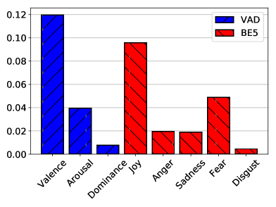
Figure 2: Relative importance of the affective variables of VAD and BE5 for predicting the alternative format, respectively; measured in drop of Pearson $r$ when using all variables vs. omitting the one under scrutiny.

Previous work has limited itself to data sets comprising all three VAD dimensions with the implicit belief that Dominance provides valuable affective information which is important for ERM. However, since only about half of the data sets developed in psychology labs (and even less provided by NLP groups) actually do comprise Dominance, this decision massively decreases the amount of data sets at hand. To resolve this dilemma, the following experiment aims at quantifying the relative importance of the different affective variables of the VAD and the BE5 format.

Our set-up works as follows: For each data set from Table 1 that includes the Dominance dimension, we trained one LR model (Section 3.1) to map VAD to BE5 and another one to map BE5 to VAD (‘dim2cat’ and ‘cat2dim’ for short) applying 10-fold cross-validation. The resulting performance measurements were averaged over all data sets.

We then repeated this procedure once for each VAD dimension (when mapping dim2cat) and each BE5 category (when mapping cat2dim), omitting one of the dimensions/categories from the source representation in every iteration, thus constituting a kind of ablation experiment. Next, for each of the “incomplete” models, we computed the difference between its performance and the performance of the “complete” model (not lacking any of the variables). Now, we can use this loss of performance as an estimate of the relative importance of the respective left-out dimension or category. The results of this experiment are depicted in Figure 2.

As can be seen, regarding VAD, Valence is by far the most important dimension with a performance drop of .12 when ablating it. In turn, Arousal, the second-best dimension only increases performance by .04, whereas Dominance contributes to less than .01 of the performance. Similarly, for Basic Emotions, Joy is the most important category, although BE5 seems to distribute the affective information more equally across its variables (with the exception of Disgust which contributes far less than .01 to the performance).

Since our data suggest that Dominance plays only a minor role within the VAD framework, we will not limit our further experiments to data sets including this dimension—as it was done in previous work (Section 2)—but rather include the large variety of bi-representational data sets which leave it out (see Table 1).

4.2 Monolingual Representation Mapping

	cat2dim				dim2cat
	WEI	LR	KNN	FFNN	WEI	LR	KNN	FFNN
en_1	.685	.841	.840	.853**	.818	.844	.868	.877***
en_2	.741	.827	.828	.843***	.821	.829	.852	.858***
es_1	.709	.856	.855	.869***	.775	.804	.849	.853***
es_2	.600	.823	.828	.844***	.797	.863	.882	.889***
es_3	.713	.799	.796	.804***	.743	.776	.820	.826***
de_1	.758	.819	.827	.837**	.701	.669	.698	.712***
pl_1	.681	.858	.870	.875**	.707	.844	.848	.855***
pl_2	.619	.803	.814	.825**	.697	.820	.834	.839**
Avg.	.688	.828	.832	.844***	.757	.806	.831	.839***

(a) Results of the monolingual experiment for the WEI baseline, two reference methods (LR and KNN) as well as our FFNN model in Pearson $r$. Best result per data set and emotion format in bold, second best result underlined; significant difference (paired two-tailed $t$-test) over the second best system marked with “*”, “**”, or “***” for $p<.05$, $.01$, or $.001$, respectively.

	Val	Aro	Dom	Joy	Ang	Sad	Fea	Dsg
en_1	.969	.741	.848	.962	.876	.871	.873	.805
en_2	.964	.704	.861	.942	.868	.821	.860	.799
es_1	.974	.771	.863	.957	.854	.833	.869	.752
es_2	.986	.828	.720	.977	.913	.867	.878	.807
es_3	.915	.692	—	.846	.839	.857	.842	.744
de_1	.929	.745	—	.894	.778	.644	.785	.461
pl_1	.963	.787	—	.946	.872	.826	.805	.826
pl_2	.947	.768	.760	.935	.844	.805	.790	.819
Avg.	.956	.754	.810	.932	.855	.816	.838	.752

(b) Results of the monolingual experiment per affective dimension in Pearson $r$. Color indicates outperforming human SHR (blue), being outperformed (red) or SHR not being reported (white; “—” meaning that the respective variable is not included).

Table 4: Results of the monolingual experiment.

In this experiment, we compared the performance of the WEI baseline, the LR- and KNN-based reference methods for ERM and our newly proposed FFNN model. For each of these methods and data sets in Table 1, we trained one model to map cat2dim and another one to map dim2cat (for the ERM methods) or to predict VA(D) ratings and BE5 ratings based on word embeddings for the WEI baseline. The whole process was conducted using 10-fold cross-validation where we used identical train/test splits for all methods. The results of this experiment are displayed in Table 4(a), only showing the average values over VA(D) and BE5, respectively, but allowing for an easy comparison between the different approaches.

As can be seen, all of the ERM approaches (LR, KNN, FFNN) perform more than 10%-points better than the state of the art in word emotion induction (WEI) for VAD prediction and at least about 5%-points better for BE5 predictions (on average over all data sets and affective variables). This finding already strongly suggests that ERM is the superior approach for automatic lexicon creation, given that the required data are available. This might be especially useful in situations where, say, large VAD but only small BE5 lexicons are available for a given language (see Section 4.4). Regarding the ordering of the ERM approaches, KNN outperforms LR in almost all cases. The advantage is more pronounced for mapping dim2cat (2.5%-points difference on average) than cat2dim (.4%-points difference). On top of that, our proposed FFNN model outperforms KNN by a 1.2%-point margin for cat2dim and a .8%-point margin for dim2cat (again as average over all data sets) performing best on each single data set. Regarding the 16 cases of Table 4(a) (8 data sets times two mapping directions), the performance gain of FFNN compared to the respective second best system is statistically significant in all but 2 cases. The differences between the individual ERM approaches might appear quite small, yet become a lot more meaningful considering the proximity to human annotation capabilities as discussed in the following paragraphs.

Table 4(b) displays the performance figures of the FFNN model relative to each affective variable. As can be seen, among VAD, Valence is the easiest dimension to predict ($r=.956$ on average over all data sets) whereas for Arousal the performance is worst . Similarly, for BE5, Joy obtains the best values ($r=.932$) and Disgust is the hardest to predict. Interestingly, the overall ordering of performance within the two formats is consistent with the ordering of human reliability (see Table 3).

Comparing our system performance against human SHR (based on 20 participants per study; see Section 3.4), again our approach seems to be highly reliable (color coding of Table 4(b)). In particular, ERM using the FFNN model outperforms SHR in over half of the applicable cases (25 of 38). For mapping cat2dim it surpasses human reliability in all but 2 cases whereas when mapping dim2cat the reported SHR is surpassed in over half of the cases (14 out of 25).

This result, astonishing as it might appear, is yet consistent with findings from previous work which, in turn, were based on ISR (not on SHR) data [Buechel and Hahn, 2017a, Buechel and Hahn, 2018a]. We conclude that in the monolingual set-up, ERM using the FFNN model substantially outperforms current capacities in word emotion induction and is even more reliable than a medium sized human rating study. Thus these automatically produced ratings should be cautiously attributed gold standard quality.

4.3 Crosslingual Representation Mapping

	Val	Aro	Joy	Ang	Sad	Fea	Dsg
en_1	.966	.683	.955	.858	.838	.817	.781
en_2	.956	.642	.934	.855	.810	.791	.800
es_1	.973	.692	.951	.786	.802	.782	.682
es_2	.985	.735	.974	.881	.860	.835	.787
es_3	.908	.548	.839	.821	.850	.807	.728
de_1	.927	.708	.889	.767	.618	.760	.458
pl_1	.957	.666	.937	.848	.784	.745	.801
pl_2	.938	.720	.932	.816	.785	.751	.809
Avg.	.951	.674	.926	.829	.793	.786	.731

Table 5: Results of crosslingual experiment in Pearson $r$. Color indicates outperforming human SHR (blue), being outperformed (red) or SHR not being reported (white).

In the crosslingual set-up, we make use of the fact that our model does not rely on any language-specific information, since the categories/dimensions describe supposedly universal affective states rather than linguistic entities. Thus, models trained on one language could, in theory, be applied to another one without any need for adaptation. This capability comes in handy when only data sets according to one emotion format exist for a given language. In such cases we could still train our model on data available for other languages and use it to produce new ratings for the language in focus. This section aims at estimating the performance of lexicons derived in this manner.

For each of the data sets in Table 1, we trained FFNN models to map cat2dim and dim2cat, respectively. We trained on each gold lexicon that did not cover the language of the data set under scrutiny (e.g., for testing on en_1, the models were trained on all Spanish, Polish and German data sets, but not on en_2). Since this set-up leads to fixed train and test sets, we did not perform cross-validation. For comparability between data sets, the Dominance dimension was excluded for this experiment.

Overall, the results remained astonishingly stable compared to the monolingual set-up, with performance figures for Valence and Joy dropping by less than 1%-point on average over all data sets (see Table 5). Also, Anger, Sadness, Fear and Disgust only suffer a moderate decrease of about 5%-points at most—only the performance of Arousal decreased more than that.

A possible explanation for these strong results is the marked increase in the amount of training data that comes along with training on the majority of the available data (independent of language). This circumstance seems to counterbalance much of the negative effects that may arise in this crosslingual applications.

In comparison to SHR, the ERM approach still turns out to work quite well. Regarding VA, we outperform human reliability in 8 of 10 cases. Concerning BE5, SHR was beaten in about half of the cases (11 of 25). We conclude that, although the capability of our mapping approach suffers a bit in the crosslingual set-up, it still produces very accurate predictions and can thus be attested near gold quality, at least.

4.4 Automatic Lexicon Construction for Diverse Languages

Mth	Lng	Format	Source	#Words
m	en	BE5	?)	12,884
m	es	VAD	?)	10,489
m	de	BE5	?)	944
m	pl	BE5	?)	3,633
c	it	BE5	?)	1,121
c	pt	BE5	?)	1,034
c	nl	BE5	?)	4,299
c	id	BE5	?)	1,487
c	zh	BE5	?); ?)	3,797
c	fr	BE5	?)	1,031
c	gr	BE5	?)	1,034
c	fn	BE5	?)	210
c	sv	BE5	?)	99

Table 6: Overview of automatically constructed emotion lexicons; mapping methodology (monolingual or crosslingual), language (codes according to ISO 639-1), target emotion format, source lexicon of the mapping process and number of previously unknown ratings (excluding those present in other lexicons).

After the positive evaluation of the FFNN model for ERM, the last bit of our contributions is to apply the created models to a wide variety of data sets which so far bear emotion ratings for one format only (either VA(D) or BE5). Based on the experiments reported so far, we claim that these have gold quality (for the monolingual approach, Section 4.2) or near-gold quality (for the crosslingual approach, Section 4.3).

For the monolingual approach, we train our model on the data set on which we achieved the highest performance in Section 4.2 for the respective language (assuming this hints at particularly “clean” data). In contrast, in the crosslingual set-up, training data are acquired by concatenating all the available data sets from Table 1 (consequently ignoring Dominance for compatibility).

Table 6 lists the emotion lexicons constructed in this manner together with their most important characteristics. The number of new ratings ranges from almost 13,000 (for English) and 10,500 (for Spanish), over several thousands (for Dutch, Chinese and Polish, ) and around 1,500–1,000 (for Indonesian, Italian, Portuguese, Greek, French and German) to 200–100 (for Finnish and Swedish). For illustration, Table 2 displays three entries of the English BE5 lexicon, the largest one we constructed.

5 Conclusion

In this paper, we addressed the relatively new task of emotion representation mapping. It aims at transforming emotion ratings for lexical units from one emotion representation format into another one, e.g., mapping from Valence-Arousal-Dominance representations to Basic Emotion ones. Based on a large-scale evaluation we gathered solid empirical evidence that the proposed neural network model consistently outperforms the previous state-of-the-art performance figures in both word emotion induction and emotion representation mapping. Hence, the approach we propose currently constitutes the best-performing method for automatic emotion lexicon creation.

We also proposed a novel methodology for comparison against human rating capabilities based on normalized split-half reliability scores. For the first time, this allows for a large-scale evaluation against human performance. Our experimental data suggest that our models perform competitive relative to human assessments, even in cross-lingual applications, thus producing (near) gold quality data. We take this as a strong hint towards the reliability of the methods we propose.

Finally, we used these models to produce new emotion lexicons for 13 typologically diverse languages which are publicly available along with our code and experimental data (see Footnote 1).

References

- [Baxter, 1997] Jonathan Baxter. 1997. A Bayesian/information theoretic model of learning to learn via multiple task sampling. Machine Learning, 28(1):7–39.
- [Bojanowski et al., 2017] Piotr Bojanowski, Edouard Grave, Armand Joulin, and Tomas Mikolov. 2017. Enriching word vectors with subword information. Transactions of the Association for Computational Linguistics, 5:135–146.
- [Bradley and Lang, 1999] Margaret M. Bradley and Peter J. Lang. 1999. Affective Norms for English Words (Anew): Stimuli, instruction manual and affective ratings. Technical Report C-1, The Center for Research in Psychophysiology, University of Florida, Gainesville, Florida, USA.
- [Briesemeister et al., 2011] Benny B. Briesemeister, Lars Kuchinke, and Arthur M. Jacobs. 2011. Discrete Emotion Norms for Nouns: Berlin Affective Word List (Denn–Bawl). Behavior Research Methods, 43(2):441.
- [Buechel and Hahn, 2016] Sven Buechel and Udo Hahn. 2016. Emotion analysis as a regression problem: Dimensional models and their implications on emotion representation and metrical evaluation. In ECAI 2016 — Proceedings of the 22nd European Conference on Artificial Intelligence. Including Prestigious Applications of Artificial Intelligence (PAIS 2016), volume 285 of Frontiers in Artificial Intelligence and Applications, pages 1114–1122, The Hague, The Netherlands, August 29 – September 2, 2016.
- [Buechel and Hahn, 2017a] Sven Buechel and Udo Hahn. 2017a. A flexible mapping scheme for discrete and dimensional emotion representations: Evidence from textual stimuli. In CogSci 2017 — Proceedings of the 39th Annual Meeting of the Cognitive Science Society, pages 180–185, London, UK, July 26–29, 2017.
- [Buechel and Hahn, 2017b] Sven Buechel and Udo Hahn. 2017b. EmoBank: Studying the impact of annotation perspective and representation format on dimensional emotion analysis. In EACL 2017 — Proceedings of the 15th Conference of the European Chapter of the Association for Computational Linguistics, volume 2, short papers, pages 578–585, Valencia, Spain, April 3–7, 2017.
- [Buechel and Hahn, 2018a] Sven Buechel and Udo Hahn. 2018a. Representation mapping: A novel approach to generate high-quality multi-lingual emotion lexicons. In LREC 2018 — Proceedings of the 11th International Conference on Language Resources and Evaluation, pages 184–191, Miyazaki, Japan, May 7–12, 2018.
- [Buechel and Hahn, 2018b] Sven Buechel and Udo Hahn. 2018b. Word emotion induction for multiple languages as a deep multi-task learning problem. In NAACL-HLT 2018 — Proceedings of the 2018 Conference of the North American Chapter of the Association for Computational Linguistics: Human Language Technologies, volume 1, long papers, pages 1907–1918, New Orleans, Louisiana, USA, June 1–6, 2018.
- [Calvo and Mac Kim, 2013] Rafael A. Calvo and Sunghwan Mac Kim. 2013. Emotions in text: Dimensional and categorical models. Computational Intelligence, 29(3):527–543.
- [Carletta, 1996] Jean C. Carletta. 1996. Assessing agreement on classification tasks: The Kappa statistic. Computational Linguistics, 22(2):249–254.
- [Caruana, 1997] Rich Caruana. 1997. Multitask learning. Machine Learning, 28(1):41–75.
- [Davidson and Innes-Ker, 2014] Per Davidson and Åse Innes-Ker. 2014. Valence and arousal norms for Swedish affective words. Technical Report Volume 14, No. 2, Lund University, Lund, Sweden.
- [Drucker, 1997] Harris Drucker. 1997. Improving regressors using boosting techniques. In ICML 1997 — Proceedings of the 14th International Conference on Machine Learning, pages 107–115, Nashville, Tennessee, USA, July 8–12, 1997.
- [Du and Zhang, 2016] Steven Du and Xi Zhang. 2016. Aicyber’s system for IALP 2016 Shared Task: Character-enhanced word vectors and boosted neural networks. In IALP 2016 — Proceedings of the 2016 International Conference on Asian Language Processing, pages 161–163, Tainan, Taiwan, November 21–23, 2016.
- [Eilola and Havelka, 2010] Tiina M. Eilola and Jelena Havelka. 2010. Affective norms for 210 British English and Finnish nouns. Behavior Research Methods, 42(1):134–140.
- [Ekman, 1992] Paul Ekman. 1992. An argument for basic emotions. Cognition & Emotion, 6(3-4):169–200.
- [Esuli and Sebastiani, 2005] Andrea Esuli and Fabrizio Sebastiani. 2005. Determining the semantic orientation of terms through gloss classification. In CIKM 2005 — Proceedings of the 14th ACM International Conference on Information and Knowledge Management, pages 617–624, Bremen, Germany, October 31 – November 05, 2005.
- [Ferré et al., 2017] Pilar Ferré, Marc Guasch, Natalia Martínez-García, Isabel Fraga, and José Antonio Hinojosa. 2017. Moved by words: Affective ratings for a set of 2,266 Spanish words in five discrete emotion categories. Behavior Research Methods, 49(3):1082–1094.
- [Hatzivassiloglou and McKeown, 1997] Vasileios Hatzivassiloglou and Kathleen R. McKeown. 1997. Predicting the semantic orientation of adjectives. In ACL-EACL 1997 — Proceedings of the 35th Annual Meeting of the Association for Computational Linguistics & 8th Conference of the European Chapter of the Association for Computational Linguistics, pages 174–181, Madrid, Spain, July 7–12, 1997.
- [Hinojosa et al., 2016a] José Antonio Hinojosa, Natalia Martínez-García, Cristina Villalba-García, Uxia Fernández-Folgueiras, Alberto Sánchez-Carmona, Miguel Angel Pozo, and Pedro R. Montoro. 2016a. Affective norms of 875 Spanish words for five discrete emotional categories and two emotional dimensions. Behavior Research Methods, 48(1):272–284.
- [Hinojosa et al., 2016b] José Antonio Hinojosa, Irene Rincón-Pérez, M. Verónica Romero-Ferreiro, Natalia Martínez-García, Cristina Villalba-García, Pedro R. Montoro, and Miguel Angel Pozo. 2016b. The Madrid Affective Database for Spanish (Mads): Ratings of dominance, familiarity, subjective age of acquisition and sensory experience. PLoS One, 11(5):e0155866.
- [Hornik, 1991] Kurt Hornik. 1991. Approximation capabilities of multilayer feedforward networks. Neural Networks, 4(2):251 – 257.
- [Imbir, 2016] Kamil K. Imbir. 2016. Affective Norms for 4900 Polish Words Reload (ANPW_R): Assessments for valence, arousal, dominance, origin, significance, concreteness, imageability and, age of acquisition. Frontiers in Psychology, 7:#1081.
- [Kingma and Ba, 2015] Diederik Kingma and Jimmy Ba. 2015. Adam: A method for stochastic optimization. In ICLR 2015 — Proceedings of the 3rd International Conference on Learning Representations, pages 1–15, San Diego, California, USA, May 7–9, 2015.
- [Köper and Schulte im Walde, 2016] Maximilian Köper and Sabine Schulte im Walde. 2016. Automatically generated affective norms of abstractness, arousal, imageability and valence for 350,000 German lemmas. In LREC 2016 — Proceedings of the 10th International Conference on Language Resources and Evaluation, pages 2595–2598, Portorož, Slovenia, May 23–28, 2016.
- [Mikolov et al., 2013] Tomas Mikolov, Ilya Sutskever, Kai Chen, Gregory S. Corrado, and Jeffrey Dean. 2013. Distributed representations of words and phrases and their compositionality. In NIPS 2013 — Proceedings of the 27th Annual Conference on Neural Information Processing Systems, pages 3111–3119, Lake Tahoe, Nevada, USA, December 5–10, 2013.
- [Mohammad and Bravo-Marquez, 2017] Saif M. Mohammad and Felipe Bravo-Marquez. 2017. Emotion intensities in tweets. In *SEM 2017 — Proceedings of the 6th Joint Conference on Lexical and Computational Semantics, pages 65–77, Vancouver, British Columbia, Canada, August 3–4, 2017.
- [Monnier and Syssau, 2014] Catherine Monnier and Arielle Syssau. 2014. Affective norms for French words (Fan). Behavior Research Methods, 46(4):1128–1137.
- [Montefinese et al., 2014] Maria Montefinese, Ettore Ambrosini, Beth Fairfield, and Nicola Mammarella. 2014. The adaptation of the Affective Norms for English Words (Anew) for Italian. Behavior Research Methods, 46(3):887–903.
- [Moors et al., 2013] Agnes Moors, Jan De Houwer, Dirk Hermans, Sabine Wanmaker, Kevin van Schie, Anne-Laura Van Harmelen, Maarten De Schryver, Jeffrey De Winne, and Marc Brysbært. 2013. Norms of valence, arousal, dominance, and age of acquisition for 4,300 Dutch words. Behavior Research Methods, 45(1):169–177.
- [Palogiannidi et al., 2016] Elisavet Palogiannidi, Polychronis Koutsakis, Elias Iosif, and Alexandros Potamianos. 2016. Affective lexicon creation for the Greek language. In LREC 2016 — Proceedings of the 10th International Conference on Language Resources and Evaluation, pages 2867–2872, Portorož, Slovenia, 23–28 May 2016.
- [Pennington et al., 2014] Jeffrey Pennington, Richard Socher, and Christopher Manning. 2014. GloVe: Global vectors for word representation. In EMNLP 2014 — Proceedings of the 2014 Conference on Empirical Methods in Natural Language Processing, pages 1532–1543, Doha, Qatar, October 25–29, 2014.
- [Pinheiro et al., 2017] Ana P. Pinheiro, Marcelo Dias, João Pedrosa, and Ana P. Soares. 2017. Minho Affective Sentences (Mas): Probing the roles of sex, mood, and empathy in affective ratings of verbal stimuli. Behavior Research Methods, 49(2):698–716.
- [Redondo et al., 2007] Jaime Redondo, Isabel Fraga, Isabel Padrón, and Montserrat Comesaña. 2007. The Spanish adaptation of Anew (Affective Norms for English Words). Behavior Research Methods, 39(3):600–605.
- [Riegel et al., 2015] Monika Riegel, Małgorzata Wierzba, Marek Wypych, Łukasz Żurawski, Katarzyna Jednoróg, Anna Grabowska, and Artur Marchewka. 2015. Nencki Affective Word List (Nawl): The cultural adaptation of the Berlin Affective Word List–Reloaded (Bawl–R) for Polish. Behavior Research Methods, 47(4):1222–1236.
- [Rosenthal et al., 2015] Sara Rosenthal, Preslav I. Nakov, Svetlana Kiritchenko, Saif M. Mohammad, Alan Ritter, and Veselin Stoyanov. 2015. SemEval 2015 Task 10: Sentiment analysis in Twitter. In SemEval 2015 — Proceedings of the 9th International Workshop on Semantic Evaluation @ NAACL-HLT 2015, pages 451–463, Denver, Colorado, USA, June 4–5, 2015.
- [Shaikh et al., 2016] Samira Shaikh, Kit Cho, Tomek Strzalkowski, Laurie Feldman, John Lien, Ting Liu, and George Aaron Broadwell. 2016. ANEW+: Automatic expansion and validation of affective norms of words lexicons in multiple languages. In LREC 2016 — Proceedings of the 10th International Conference on Language Resources and Evaluation, pages 1127–1132, Portorož, Slovenia, 23–28 May 2016.
- [Sianipar et al., 2016] Agnes Sianipar, Pieter van Groenestijn, and Ton Dijkstra. 2016. Affective meaning, concreteness, and subjective frequency norms for Indonesian words. Frontiers in Psychology, 7:#1907.
- [Soares et al., 2012] Ana Paula Soares, Montserrat Comesaña, Ana P. Pinheiro, Alberto Simões, and Carla Sofia Frade. 2012. The adaptation of the Affective Norms for English Words (Anew) for European Portuguese. Behavior Research Methods, 44(1):256–269.
- [Srivastava et al., 2014] Nitish Srivastava, Geoffrey E. Hinton, Alex Krizhevsky, Ilya Sutskever, and Ruslan Salakhutdinov. 2014. Dropout: A simple way to prevent neural networks from overfitting. Journal of Machine Learning Research, 15:1929–1958.
- [Stadthagen-González et al., 2017a] Hans Stadthagen-González, Pilar Ferré, Miguel A. Pérez-Sánchez, Constance Imbault, and José Antonio Hinojosa. 2017a. Norms for 10,491 Spanish words for five discrete emotions: Happiness, disgust, anger, fear, and sadness. Behavior Research Methods. Available: https://doi.org/10.3758/s13428-017-0962-y.
- [Stadthagen-Gonzalez et al., 2017b] Hans Stadthagen-Gonzalez, Constance Imbault, Miguel A. Pérez-Sánchez, and Marc Brysbært. 2017b. Norms of valence and arousal for 14,031 Spanish words. Behavior Research Methods, 49(1):111–123.
- [Stevenson et al., 2007] Ryan A. Stevenson, Joseph A. Mikels, and Thomas W. James. 2007. Characterization of the Affective Norms for English Words by discrete emotional categories. Behavior Research Methods, 39(4):1020–1024.
- [Strapparava and Mihalcea, 2007] Carlo Strapparava and Rada Mihalcea. 2007. SemEval 2007 Task 14: Affective text. In SemEval 2007 — Proceedings of the 4th International Workshop on Semantic Evaluations @ ACL 2007, pages 70–74, Prague, Czech Republic, June 23–24, 2007.
- [Turney and Littman, 2003] Peter D. Turney and Michael L. Littman. 2003. Measuring praise and criticism: Inference of semantic orientation from association. ACM Transactions on Information Systems, 21(4):315–346.
- [Võ et al., 2009] Melissa L. H. Võ, Markus Conrad, Lars Kuchinke, Karolina Urton, Markus J. Hofmann, and Arthur M. Jacobs. 2009. The Berlin Affective Word List Reloaded (Bawl–R). Behavior Research Methods, 41(2):534–538.
- [Vet et al., 2017] Henrica C. W. de Vet, Lidwine B. Mokkink, David G. Mosmuller, and Caroline B. Terwee. 2017. Spearman-Brown prophecy formula and Cronbach’s alpha: Different faces of reliability and opportunities for new applications. Journal of Clinical Epidemiology, 85:45–49.
- [Warriner et al., 2013] Amy Beth Warriner, Victor Kuperman, and Marc Brysbært. 2013. Norms of valence, arousal, and dominance for 13,915 English lemmas. Behavior Research Methods, 45(4):1191–1207.
- [Wierzba et al., 2015] Małgorzata Wierzba, Monika Riegel, Marek Wypych, Katarzyna Jednoróg, Paweł Turnau, Anna Grabowska, and Artur Marchewka. 2015. Basic emotions in the Nencki Affective Word List (Nawl BE): New method of classifying emotional stimuli. PLoS One, 10(7):e0132305.
- [Yao et al., 2017] Zhao Yao, Jia Wu, Yanyan Zhang, and Zhenhong Wang. 2017. Norms of valence, arousal, concreteness, familiarity, imageability, and context availability for 1,100 Chinese words. Behavior Research Methods, 49(4):1374–1385.
- [Yu et al., 2016a] Liang-Chih Yu, Lung-Hao Lee, Shuai Hao, Jin Wang, Yunchao He, Jun Hu, K. Robert Lai, and Xuejie Zhang. 2016a. Building Chinese affective resources in valence-arousal dimensions. In NAACL-HLT 2016 — Proceedings of the 2016 Conference of the North American Chapter of the Association for Computational Linguistics: Human Language Technologies, pages 540–545, San Diego, California, USA, June 12–17, 2016.
- [Yu et al., 2016b] Liang-Chih Yu, Lung-Hao Lee, and Kam-Fai Wong. 2016b. Overview of the IALP 2016 Shared Task on dimensional sentiment analysis for Chinese words. In IALP 2016 — Proceedings of the 2016 International Conference on Asian Language Processing, pages 156–160, Tainan, Taiwan, November 21–23, 2016.