Surface-induced non-equilibrium dynamics and critical Casimir forces
for model B in film geometry

Abstract

Using analytic and numerical approaches, we study the spatio-temporal evolution of a conserved order parameter of a fluid in film geometry, following an instantaneous quench to the critical temperature $T_{c}$ as well as to supercritical temperatures. The order parameter dynamics is chosen to be governed by model B within mean field theory and is subject to no-flux boundary conditions as well as to symmetric surface fields at the confining walls. The latter give rise to critical adsorption of the order parameter at both walls and provide the driving force for the non-trivial time evolution of the order parameter. During the dynamics, the order parameter is locally and globally conserved; thus, at thermal equilibrium, the system represents the canonical ensemble. We furthermore consider the dynamics of the nonequilibrium critical Casimir force, which we obtain based on the generalized force exerted by the order parameter field on the confining walls. We identify various asymptotic regimes concerning the time evolution of the order parameter and the critical Casimir force and we provide, within our approach, exact expressions of the corresponding dynamic scaling functions.

I Introduction

A fluid at its critical point exhibits scale-invariant long-ranged fluctuations and a drastic slowing-down of its dynamics. The critical behavior is characterized by universal features which are determined by general properties of the fluid, such as the dimensionality of the order parameter (OP), conservation laws, and possibly secondary fields coupled to the OP Hohenberg and Halperin (1977). We recall that, in a one-component fluid, the OP $\phi$ is proportional to the deviation of the actual number density $n$ from its critical value $n_{c}$, i.e., $\phi\propto n-n_{c}$, while for a binary liquid mixture, $\phi$ is proportional to the deviation of the concentration $C_{A}$ of species A from its critical value $C_{A,c}$, i.e., $\phi\propto C_{A}-C_{A,c}$.

Dynamic critical phenomena have been extensively studied in bulk fluids (see, e.g., Refs. Folk and Moser (2006); Täuber (2014) for reviews) and in a semi-infinite geometry Dietrich and Diehl (1983); Diehl and Janssen (1992); Diehl (1994); Wichmann and Diehl (1995); Ritschel and Czerner (1995); Majumdar and Sengupta (1996); Pleimling (2004). However, in the case of more strongly confined systems, such as films, theoretical results on dynamic criticality are more scarce. In fact, previous studies Diehl and Ritschel (1993); Ritschel and Diehl (1995, 1996); Gambassi and Dietrich (2006); Diehl and Chamati (2009); Gambassi (2008) mostly addressed purely relaxational dynamics, i.e., model A in the nomenclature of Ref. Hohenberg and Halperin (1977), which captures the dynamics of a single non-conserved density, e.g., the magnetization in the case of a uniaxial ferromagnet near its Curie point. The critical dynamics of a fluid, instead, is described by model H, which, in its simplest realization, encompasses an advection-diffusion equation for the conserved OP, coupled to a diffusive transport equation for the transverse fluid momentum Hohenberg and Halperin (1977). In passing, we mention that a significant number of studies of (partly) confined fluids exists addressing specific sub-critical phenomena, such as surface-induced phase separation Ball and Essery (1990); Binder and Frisch (1991); Puri and Frisch (1993); Lee et al. (1999); Onuki (2002).

Introducing confinement in a near-critical fluid gives rise to the so-called critical Casimir force (CCF) acting on the confining boundaries Fisher and de Gennes (1978); Krech and Dietrich (1992). Generally, the CCF can result from a confinement-induced long-wavelength cutoff of the fluctuation spectrum as well as from the appearance of slowly decaying OP profiles in the film (see, e.g., Refs. Krech (1994); Brankov et al. (2000); Gambassi (2009) for reviews). In the latter case, the CCF lends itself to a description within mean field theory (MFT), which entails neglecting effects of thermal noise. Similarly to critical dynamics, studies on the dynamics of thermal Casimir-like forces in films focused so far mostly on model A Gambassi and Dietrich (2006); Brito et al. (2007); Gambassi (2008); Rodriguez-Lopez et al. (2011); Dean and Gopinathan (2010); Dean et al. (2012); Dean and Podgornik (2014); Hanke (2013), with the exception of Ref. Rohwer et al. (2017), where model B-like dynamics in a quench far from criticality has been investigated.

Here, we consider a film after an instantaneous quench from a quasi-infinite temperature right to the critical point as well as to supercritical temperatures. Thus in the initial state the mean OP profile across the film vanishes Gross et al. (2016). However, at finite temperatures, the presence of effective surface fields at the confining walls gives rise to the build-up of a spatially varying adsorption profile across the film at late times ($t\to\infty$). Accordingly, in the present MFT case the dynamics of the OP and of the resulting CCF is induced solely by the action of surface fields. In order to facilitate an analytical study, we approximate the actual critical fluid dynamics in terms of the mean-field limit of model B, which describes the diffusive dynamics of a single conserved OP but neglects fluctuations. Accordingly, we also assume heat diffusion to be sufficiently fast to provide an effective isothermal environment directly after the quench.

In Ref. Gross et al. (2016) it has been shown that in a film, which is close to criticality and confined by the walls of the container, the behavior of the equilibrium CCF depends crucially on whether the OP of the confined fluid is conserved or not. In particular, for so-called $(++)$ boundary conditions, i.e., if the confined fluid is adsorbed with equal strength at both walls, the CCF is attractive in the grand canonical ensemble (globally non-conserved OP), while it is repulsive in the canonical ensemble (globally conserved OP). For model B dynamics in a film with no-flux boundary conditions, the total OP is conserved at all times, i.e.,

$$\Phi(t)\equiv\int_{V}\mathrm{d}^{d}r\,\phi(t,\mathbf{r})=\mathrm{const},$$ (1)

where the integral runs over the $d$-dimensional volume $V$ of the film. In Ref. Gross et al. (2017), ensemble-induced differences for the CCF have been discussed within a field theoretical treatment and for further boundary conditions. In the present study, we investigate how the equilibrium CCF in the canonical ensemble considered in Ref. Gross et al. (2016) emerges dynamically within model B after a temperature quench.

II General scaling considerations

Here, we formulate the general dynamic scaling behavior expected for the OP and the CCF for a confined fluid (see, e.g., Refs. Diehl (1986); Gambassi and Dietrich (2006); Gross et al. (2016)). We consider systems which are translationally invariant along the lateral film directions, such that, as a consequence of the mean-field approximation, only the transverse coordinate $z$ enters the description. We consider symmetric [$(++)$] boundary conditions, such that the influence of the confining walls, placed at $z=0$ and $z=L$, is accounted for by a single parameter $h_{1}$, describing the strength of both surface fields. In a near-critical film of thickness $L$, the OP $\phi$ fulfills the general homogeneity relation

$$\phi(t,z,\tau,h_{1},L)=b^{-\beta/\nu}\phi(tb^{-\mathpzc{z}},z/b,\tau b^{1/\nu},h_{1}b^{\Delta_{1}/\nu},L/b)$$ (2)

where $b$ is a scaling factor,

$$\tau\equiv\frac{T-T_{c}}{T_{c}}$$ (3)

is the reduced temperature, $\beta$ and $\nu$ are standard bulk critical exponents, $\Delta_{1}$ is a surface critical exponent Gross et al. (2016); Diehl (1986), and $\mathpzc{z}$ (not to be confused with the spatial coordinate $z$) is the dynamic bulk critical exponent. In model B, one has $\mathpzc{z}=4-\eta$, where $\eta$ is a standard static critical exponent Täuber (2014); Hohenberg and Halperin (1977). Within MFT, one has $\eta=0$ and thus

$$\mathpzc{z}=4.$$ (4)

Upon setting $b=L$ in Eq. 2 and by introducing appropriate length and time scales, one obtains the following finite-size scaling relation Gross et al. (2016); Gambassi and Dietrich (2006):

$$\phi(t,z,\tau,h_{1},L)=\phi_{t}^{(0)}\left(\frac{L}{\xi_{+}^{(0)}}\right)^{-\beta/\nu}\mathpzc{m}(\theta,\zeta,x,H_{1})$$ (5)

where $\mathpzc{m}$ is a universal scaling function. We have introduced the following scaling variables:

$$\zeta \equiv z/L,$$ (6a)

$$x \equiv\left(\frac{L}{\xi_{+}^{(0)}}\right)^{1/\nu}\tau\,=\left(\frac{L}{\xi}\right)^{1/\nu},$$ (6b)

$$H_{1} \equiv\left(\frac{L}{l_{h_{1}}^{(0)}}\right)^{\Delta_{1}/\nu}h_{1},$$ (6c)

$$\theta \equiv\left(\frac{\xi_{+}^{(0)}}{L}\right){z}\frac{t}{\mathpzc{t}_{+}^{(0)}}=\left(\frac{\xi}{L}\right){z}\tau^{\nu\mathpzc{z}}\frac{t}{\mathpzc{t}_{+}^{(0)}}\,=\left(\frac{\tau}{x}\right)^{\nu\mathpzc{z}}\frac{t}{\mathpzc{t}_{+}^{(0)}}.$$ (6d)

The non-universal amplitudes $\xi_{+}^{(0)}$ and $\phi_{t}^{(0)}$ are defined in terms of the critical behavior of the bulk correlation length $\xi$ above $T_{c}$, i.e., $\xi(\tau\to 0)=\xi_{+}^{(0)}\tau^{-\nu}$, and of the bulk OP $\phi_{b}$ below $T_{c}$, i.e., $\phi_{b}=\phi_{t}^{(0)}(-\tau)^{\beta}$. The non-universal amplitude $l_{h_{1}}^{(0)}$ relates the characteristic length scale $l_{h_{1}}$ for the OP decay close to the wall (i.e., the so-called “extrapolation length”) to the strength $h_{1}$ of the effective surface field via $l_{h_{1}}=l_{h_{1}}^{(0)}|h_{1}|^{-\nu/\Delta_{1}}$ (see Ref. Gross et al. (2016) for further details). The non-universal amplitude $\mathpzc{t}_{+}^{(0)}$ is defined via the critical divergence of the relaxation time $t_{R}$ above $T_{c}$, i.e., $t_{R}=\mathpzc{t}_{+}^{(0)}\tau^{-\nu\mathpzc{z}}$. The bulk correlation length and the relaxation time can be inferred from the exponential decay in space and time of the dynamical bulk correlation function.

In thermal equilibrium, the CCF $\mathcal{K}$ can be defined as the difference of the thermodynamic pressure $p_{f}=-\mathrm{d}\mathcal{F}_{f}/\mathrm{d}L$ of the film and the pressure $p_{b}$ of the surrounding bulk medium:

$$\mathcal{K}_{\text{eq}}=p_{f}-p_{b}.$$ (7)

Here, $\mathcal{F}_{f}$ denotes the total free energy of the film (per area $A$ of a single wall and $k_{B}T$), while the bulk pressure is obtained as $p_{b}=\lim_{L\to\infty}p_{f}$. Note that the limit is to be performed by keeping the relevant thermodynamic control parameter fixed, which is the external bulk field $\mu$ in the grand canonical ensemble and the mean mass density $\Phi/(AL)$ [see Eq. 1] in the canonical ensemble. In the presence of an OP constraint, the definition of the CCF is, in fact, subtle and we refer to Ref. Gross et al. (2016) for further discussion. In Sec. VI, we shall extend the definition of the CCF to non-equilibrium situations and we shall show that this definition reduces to Eq. 7 in the equilibrium limit.

Since near criticality the correlation length $\xi$ and the relaxation time $t_{R}$ represent the dominant length and time scales, one expects a scaling form analogous to Eq. 5 to apply also for the general non-equilibrium CCF $\mathcal{K}$, i.e.,

$$\mathcal{K}(t,\tau,h_{1})=L^{-d}\Xi(\theta,x,H_{1}),$$ (8)

where $\Xi$ is a scaling function and the scaling variables $\theta$, $x$, and $H_{1}$ are given in Eq. 6.

III Model

In this section we introduce the dynamic model to be analyzed below. In the following all extensive quantities are understood to be divided by the transverse area $A$. Within our approach the static properties of the OP field $\phi(t,z)$ follow from the standard Landau-Ginzburg free energy functional (defined per area and per $k_{B}T$):

$$\mathcal{F}[\phi]=\int_{0}^{L}\mathrm{d}z\,\left[(\partial_{z}\phi)^{2}+\mathcal{U}_{b}(\phi)+\mathcal{U}_{s}(\phi)\right],$$ (9)

where

$$\mathcal{U}_{b}(\phi)\equiv\frac{r}{2}\phi^{2}+\frac{g}{4!}\phi^{4}$$ (10)

and

$$\mathcal{U}_{s}(\phi)\equiv\left[\frac{1}{2}c\phi^{2}-h_{1}\phi\right]\left[\delta(z)+\delta(z-L)\right]$$ (11)

denote the bulk and the surface contribution, respectively. In Eq. 9, the integral runs from $z=0^{-}$ up to $z=L^{+}$. Within MFT, the coupling constants $r=(\xi_{+}^{(0)})^{-2}\tau$ and $g=6(\phi_{t}^{(0)}\xi_{+}^{(0)})^{-2}$ are given in terms of the non-universal amplitudes $\xi_{+}^{(0)}$ and $\phi_{t}^{(0)}$ introduced in Eqs. 5 and 6 Pelissetto and Vicari (2002). The parameters $c$ and $h_{1}$ in Eq. 11 represent the surface enhancement and the surface adsorption strength for the OP, respectively. Here, we focus on the case $c=0$ and $h_{1}>0$, corresponding to the $(++)$ surface universality class, which describes critical adsorption as observed generically for a confined fluid Gambassi et al. (2009). Minimization of $\mathcal{F}$ leads to the well-known equilibrium boundary conditions Gross et al. (2016)

$$\partial_{z}\phi(t,z=0)=-h_{1}\qquad\text{and}\qquad\partial_{z}\phi(t,z=L)=h_{1},$$ (12)

which we will impose also during the non-equilibrium time evolution.

The dynamics of $\phi$ is governed by model B, which, within MFT, is given by Hohenberg and Halperin (1977)

$$\partial_{t}\phi=-\partial_{z}J=D\partial_{z}^{\,2}\mu=D\left\{-\partial_{z}^{\,4}\phi+\partial_{z}^{\,2}\left[\mathcal{U}_{b}^{\prime}(\phi)\right]\right\}.$$ (13)

Here, the diffusivity $D$ is a kinetic coefficient, $J\equiv-D\partial_{z}\mu$ is the flux, and

$$\mu\equiv\frac{\delta\mathcal{F}_{b}}{\delta\phi}=-\partial_{z}^{2}\phi+r\phi+\frac{g}{3!}\phi^{3}$$ (14)

is the bulk chemical potential, defined in terms of the corresponding bulk free energy functional $\mathcal{F}_{b}\equiv\mathcal{F}-\int_{0}^{L}\mathrm{d}z\,\mathcal{U}_{s}(\phi)$. In order to ensure global mass conservation, no-flux boundary conditions are imposed, i.e., $J(t,z=0)=0=J(t,z=L)$, or, equivalently,

$$0=-\partial_{z}\mu=\partial_{z}^{3}\phi(t,z)-\left[r+\frac{g}{2}\phi^{2}(t,z)\right]\partial_{z}\phi(t,z),\quad\text{for}\quad z=0,L.$$ (15)

The boundary conditions in Eqs. 12 and 15 are imposed at all times $t>0$. They have also been derived in Ref. Diehl and Janssen (1992) within a full field theoretical treatment of model B in a half-space.

We focus on the dynamics induced by Eq. 13 after an instantaneous quench from a high temperature ($\tau\to\infty$) to a temperature close to $T_{c}$. In the limit $\tau\to\infty$ the equilibrium OP profile resulting from Eq. 9 vanishes so that, accordingly, the initial condition is

$$\phi(t=0,z)=0.$$ (16)

In the course of time, the OP profile attains its equilibrium shape characteristic for critical adsorption under $(++)$ boundary conditions Gross et al. (2016). In the present case, owing to no-flux boundary conditions [Eq. 15], the OP is globally conserved. Equation 16 therefore implies

$$\int_{0}^{L}\mathrm{d}z\,\phi(t,z)=0,$$ (17)

i.e., the so-called “mass” $\Phi(t)$ [per area $A$, see Eq. 1] vanishes at all times $t$.

Within MFT, the dynamical critical exponent is $\mathpzc{z}=4$ [Eq. 4] and the finite-size scaling variables in Eqs. 5 and 6 take the forms

$$\zeta =z/L,$$ (18a)

$$x =L^{2}r,$$ (18b)

$$H_{1} =\sqrt{\frac{g}{6}}L^{2}h_{1},$$ (18c)

$$\theta =\frac{D}{L^{4}}t,$$ (18d)

$$\mathpzc{m}(\theta,\zeta) =\sqrt{\frac{g}{6}}L\phi\left(L^{4}\theta/D,\zeta L\right).$$ (18e)

According to Eq. 6d, the kinetic coefficient $D$ can be expressed in terms of non-universal amplitudes as $D=(\xi_{+}^{(0)})^{4}/\mathpzc{t}_{+}^{(0)}$. Using Eq. 18, the dynamic equation of model B [Eq. 13] assumes the dimensionless form

$$\partial_{\theta}\mathpzc{m}=\partial_{\zeta}^{2}\left(-\partial_{\zeta}^{2}\mathpzc{m}+x\,\mathpzc{m}+\mathpzc{m}^{3}\right)$$ (19)

and the boundary conditions in Eqs. 12 and 15 become

$$\partial_{\zeta}\mathpzc{m}(\theta,\zeta=0)=-H_{1},\qquad\partial_{\zeta}\mathpzc{m}(\theta,\zeta=1) =H_{1},$$ (20a)

$$\partial_{\zeta}^{3}\mathpzc{m}(\theta,\zeta)-\left[x+3\mathpzc{m}^{2}(\theta,\zeta)\right]\partial_{\zeta}\mathpzc{m}(\theta,\zeta) =0,\quad\text{for}\quad\zeta=0,1.$$ (20b)

In the following we proceed with an analysis of this set of equations.

IV Linear quench dynamics

In order to facilitate an analytical study of Eq. 19, in the free energy functional [Eq. 10] we disregard the term $\propto\phi^{4}$. This amounts to studying the linearized (or Gaussian) model B,

$$\partial_{\theta}\mathpzc{m}=-\partial_{\zeta}^{4}\mathpzc{m}+x\partial_{\zeta}^{2}\mathpzc{m},$$ (21)

together with Eq. 12 and the linearized no-flux boundary condition in Eq. 20b, i.e., $\partial_{\zeta}^{3}\mathpzc{m}-x\partial_{\zeta}\mathpzc{m}=0$. Upon introducing the Laplace transform

$$\hat{\mathpzc}{m}(s,\zeta)=\int_{0}^{\infty}\mathrm{d}\theta\,\mathpzc{m}(\theta,\zeta)e^{-s\theta},$$ (22)

Eq. 21 turns into

$$s\hat{\mathpzc}{m}(s,\zeta)=\mathpzc{m}(\theta=0,\zeta)-\partial_{\zeta}^{4}\hat{\mathpzc}{m}(s,\zeta)+x\partial_{\zeta}^{2}\hat{\mathpzc}{m}(s,\zeta).$$ (23)

Assuming as initial condition a flat profile $\mathpzc{m}(\theta=0,\zeta)=0$ [see Eq. 16], Eq. 23 reduces to a homogeneous fourth-order differential equation:

$$s\hat{\mathpzc}{m}(s,\zeta)=-\partial_{\zeta}^{4}\hat{\mathpzc}{m}(s,\zeta)+x\partial_{\zeta}^{2}\hat{\mathpzc}{m}(s,\zeta).$$ (24)

This equation is solved by the ansatz $\mathpzc{m}(s,\zeta)\propto\exp(\Omega\zeta)$, with the parameter $\Omega$ taking one of the four possible values $\{\lambda_{\pm},-\lambda_{\pm}\}$ where

$$\lambda_{\pm}=\frac{1}{\sqrt{2}}\sqrt{x\pm\sqrt{x^{2}-4s}}.$$ (25)

Imposing the (linearized version of the) boundary conditions in Eq. 20 yields

$$\hat{\mathpzc}{m}(s,\zeta)/H_{1}=\frac{x-\lambda_{+}^{2}}{s\left(e^{\lambda_{-}}-1\right)\lambda_{-}(\lambda_{-}^{2}-\lambda_{+}^{2})}\left[e^{\zeta\lambda_{-}}+e^{(1-\zeta)\lambda_{-}}\right]+\frac{x-\lambda_{-}^{2}}{s\left(e^{\lambda_{+}}-1\right)\lambda_{+}(\lambda_{+}^{2}-\lambda_{-}^{2})}\left[e^{\zeta\lambda_{+}}+e^{(1-\zeta)\lambda_{+}}\right]$$ (26)

as the solution of Eq. 24. Since Eq. 26 has only a simple pole in $s$, at $s=0$, the long-time limit follows from Eq. 26 as Poularikas (2010)

$$\mathpzc{m}_{\text{eq}}(\zeta)\equiv\mathpzc{m}(\theta\to\infty,\zeta)=\lim_{s\to 0^{+}}s\hat{\mathpzc}{m}(s,\zeta)=\frac{H_{1}}{x}\left(\sqrt{x}\frac{\cosh\left[\left(1/2-\zeta\right)\sqrt{x}\,\right]}{\sinh\left(\sqrt{x}/2\right)}-2\right)$$ (27)

corresponding, in unrescaled quantities, to

$$\phi_{\text{eq}}(z)=\frac{h_{1}}{Lr}\left(L\sqrt{r}\frac{\cosh\left[\left(L/2-z\right)\sqrt{r}\,\right]}{\sinh\left(L\sqrt{r}/2\right)}-2\right).$$ (28)

These expressions agree with the ones obtained by minimizing the equilibrium free energy in Eq. 9 under the constraint of vanishing total mass, $\int_{0}^{L}\mathrm{d}z\,\phi_{\text{eq}}(\zeta)=0$ Gross et al. (2016). For later use, we determine $\mathpzc{m}_{\text{eq}}$ in a few particular limits. At criticality (i.e., $x=0$), Eq. 27 reduces to

$$\mathpzc{m}_{\text{eq}}(\zeta)\big{|}_{x=0}=H_{1}\left(\frac{1}{6}-\zeta+\zeta^{2}\right),$$ (29)

and, for general $x\geq 0$ and at $\zeta=0$, to

$$\mathpzc{m}_{\text{eq}}(\zeta=0)\big{|}_{x\geq 0}=H_{1}\left[\frac{\coth(\sqrt{x}/2)}{\sqrt{x}}-\frac{2}{x}\right].$$ (30)

Asymptotically for $x\to\infty$, instead, the OP profile behaves as

$$\mathpzc{m}_{\text{eq}}(\zeta)\big{|}_{x\gg 1}\simeq\frac{H_{1}}{\sqrt{x}}\left(e^{-\zeta\sqrt{x}}+e^{-(1-\zeta)\sqrt{x}}\right).$$ (31)

We remark that, within linear MFT, the strength $H_{1}$ of the surface field appears as an overall prefactor in the expression for the OP profile. Within nonlinear MFT, the limit $H_{1}\to\infty$, corresponding to the fixed-point of the critical adsorption universality class Diehl (1986), is ill-defined in the presence of the global OP conservation (see Ref. Gross et al. (2016)). In fact, studying the limit $H_{1}\to\infty$ requires to include thermal fluctuations, which is beyond the scope of the present study.

Using Eq. 27, the solution for the OP profile can be conveniently written as

$$\hat{\mathpzc}{m}(s,\zeta)=\frac{\mathpzc{m}_{\text{eq}}(\zeta)}{s}+\hat{\psi}(s,\zeta),$$ (32)

where the first term describes the equilibrium profile and $\hat{\psi}$ encodes the relaxation towards it. The function $\hat{\psi}(s,\zeta)$ has a regular expansion around $s=0$ in terms of positive integer powers of $s$ and, therefore, it is defined over the whole complex plane without a branch cut. The time dependence of $\mathpzc{m}$ follows from the inverse Laplace transform of $\hat{\mathpzc}{m}$, i.e.,

$$\mathpzc{m}(\theta,\zeta)=\frac{1}{2\pi\mathrm{i}}\int_{\mathcal{C}}\mathrm{d}s\,\hat{\mathpzc}{m}(s,\zeta)e^{s\theta},$$ (33)

where the contour $\mathcal{C}$ runs parallel to the imaginary axis and to the right of the pole of $\hat{\mathpzc}{m}$ at $s=0$. Inserting Eq. 32 into Eq. 33, the contribution from the pole at $s=0$ renders $\mathpzc{m}_{\text{eq}}(\zeta)$ as the residue. The contribution involving $\hat{\psi}$ reduces to an inverse Fourier transform since the contour $\mathcal{C}$ can be shifted onto the imaginary axis. One accordingly obtains

$$\mathpzc{m}(\theta,\zeta)=\mathpzc{m}_{\text{eq}}(\zeta)+\frac{1}{2\pi}\int_{-\infty}^{\infty}\mathrm{d}v\,\hat{\psi}(\mathrm{i}v,\zeta)e^{\mathrm{i}v\theta}$$ (34)

where the second term on the r.h.s. must vanish as $\theta\to\infty$.

Closed analytical expressions for the Laplace inversion in Eq. 33 can be obtained in certain asymptotic limits, which are discussed in the following sections. In the general case, the Laplace inversion has to be computed numerically. An efficient and robust approach, which we use here, is provided by the Talbot method Abate and Valkó (2004).

IV.1 Quench to the critical point ($x=0$)

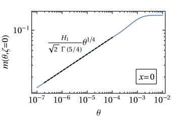
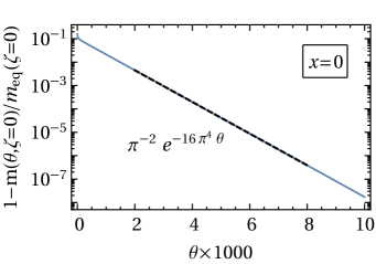
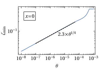
Figure 1: Time-evolution of the OP profile $m(\theta,\zeta)$, subject to the linearized model B dynamics according to Eqs. 21, 20a, and 20b and to the initial condition Eq. 16, at criticality $x=0$ [see Eq. 18b]. (a) Profile shape for times $\theta=10^{-6},3\times 10^{-5},3\times 10^{-4},\infty$ corresponding to the solid (blue), dashed (orange), dotted (red), and dashed-dotted (black) curves, respectively. For $\theta\gtrsim 10^{-2}$, the OP has essentially reached equilibrium. (b) OP at the wall at early times $\theta\lesssim\theta^{*}_{e}\simeq 10^{-4}$ [see Eq. 41]. The dashed (black) line indicates the asymptotic result in Eq. 44. (c) OP at the wall at late times $\theta\gtrsim\theta^{*}_{e}$. The dashed (black) line indicates the asymptotic result in Eq. 42. (d) Short-time scaling function of the profile, obtained asymptotically for $\zeta\to 0$ and for short times $\theta\to 0$, as function of the scaling variable $\Theta=\zeta/\theta^{1/4}$ [Eq. 49]. (e) Position $\zeta_{\text{min}}$ of the global minimum of the OP profile for $0\leq\zeta<1/2$ as a function of the rescaled time $\theta$, as determined numerically via the Laplace inversion of Eq. 36. The dashed (black) line represents the prediction given in Eq. 47.

For $x=0$, Eq. 25 reduces to

$$\lambda_{\pm}=\frac{1}{\sqrt{2}}(\pm 1+\mathrm{i})s^{1/4}$$ (35)

and the expression for the profile in Laplace space given in Eq. 26 becomes

$$\hat{\mathpzc}{m}(s,\zeta)=\frac{H_{1}}{2\omega^{5}}\big{[}\cos(\omega\zeta)\cot(\omega/2)-\cosh(\omega\zeta)\coth(\omega/2)+\sin(\omega\zeta)+\sinh(\omega\zeta)\big{]}$$ (36)

where we introduced

$$\omega\equiv(-s)^{1/4}=\lambda_{+}=s^{1/4}\exp(\mathrm{i}\pi/4).$$ (37)

For definiteness, we consider $(-1)^{1/4}=e^{\mathrm{i}\pi/4}$ as the principal branch of the complex root. Since all physical quantities considered here are real-valued, they are not affected by this particular choice. Figure 1 illustrates the time evolution of the scaled profile $\mathpzc{m}(\theta,\zeta)$ for the linearized model B and for $x=0$ as determined by the numerical Laplace inversion of Eq. 36. The profile starts from a flat configuration [Eq. 16, not shown] and evolves towards the equilibrium solution given in Eq. 29 (dashed-dotted curve). We proceed with an analysis of the characteristic spatial and temporal scaling behavior of the profile.

IV.1.1 Order parameter at the boundary: $\mathpzc{m}(\theta,\zeta=0)$

In order to determine the time evolution of the profile at the boundary, we evaluate Eq. 36 at $\zeta=0$:

$$\hat{\mathpzc}{m}(s,\zeta=0)=\frac{H_{1}}{2\omega^{5}}\left[\cot(\omega/2)-\coth(\omega/2)\right].$$ (38)

In order to determine the Laplace inversion of this expression, we expand the functions $\cot$ and $\coth$ in terms of simple fractions (see §1.42 in Ref. Gradshteyn and Ryzhik (2014)), resulting in

$$\hat{\mathpzc}{m}(s,\zeta=0)=\frac{H_{1}}{\omega^{4}}\sum_{k=1}^{\infty}\frac{16\pi^{2}k^{2}}{\omega^{4}-16\pi^{4}k^{4}}$$ (39)

and finally

$$\mathpzc{m}(\theta,\zeta=0)=H_{1}\left[\frac{1}{6}-\sum_{k=1}^{\infty}\frac{\exp(-16\pi^{4}k^{4}\theta)}{\pi^{2}k^{2}}\right],$$ (40)

where we used $\sum_{k=1}^{\infty}k^{-2}=\pi^{2}/6$. The first term on the r.h.s. can be identified with $\mathpzc{m}_{\text{eq}}(\zeta=0)$ [see Eq. 29]. We note that the expression in Eq. 40 occurs in similar form in various contexts and its asymptotic behavior has been analyzed previously (see Ref. Gross (2018) and references therein). For times $\theta\gg\theta^{*}_{e}$, with

$$\theta^{*}_{e}\simeq\frac{1}{16\pi^{4}}\sim\mathcal{O}(10^{-4}),$$ (41)

the term for $k=1$ in Eq. 40 dominates the sum, implying that

$$\mathpzc{m}(\theta\gg 1,\zeta=0)\simeq\mathpzc{m}_{\text{eq}}(0)-\frac{1}{6\pi^{2}}H_{1}e^{-16\pi^{4}\theta}$$ (42)

provides the late-time asymptotic behavior of the OP. The asymptotic behavior of Eq. 40 for $\theta\to 0$ can be obtained by replacing the sum by an integral, i.e.,

$$\mathpzc{m}(\theta\to 0,\zeta=0)\simeq H_{1}\int_{0}^{\infty}\mathrm{d}k\frac{1-\exp(-16\pi^{4}k^{4}\theta)}{\pi^{2}k^{2}}=\theta^{1/4}\frac{H_{1}}{2\pi}\int_{0}^{\infty}\mathrm{d}p\frac{1-e^{-p}}{p^{5/4}}.$$ (43)

Numerical analysis shows that this approximation is reliable up to times $\theta\simeq\theta^{*}_{e}$, such that the asymptotic early-time behavior of the OP at the wall results, upon evaluating the integral in Eq. 43, as

$$\mathpzc{m}(\theta,\zeta=0)\simeq\frac{H_{1}}{\sqrt{2}\,\Gamma(5/4)}\theta^{1/4},\qquad\theta\lesssim\theta^{*}_{e}.$$ (44)

The early-time and late-time behavior of the OP at the wall for $x=0$ are illustrated in Fig. 1(b) and (c), respectively, where we find excellent agreement between the numerical Laplace inversion of Eq. 38 (solid curves) and the asymptotic results in Eqs. 42 and 44 (dashed lines).

IV.1.2 Short-time scaling function of the profile

Next we consider the full spatio-temporal evolution of the profile [Eq. 36] at short times near one wall, i.e., for $\theta\to 0$ and $0<\zeta\ll 1/2$. Inserting Eq. 36 into Eq. 33 and changing the integration variable to $\sigma=s\theta$ yields

$$\mathpzc{m}(\theta,\zeta)=\theta^{1/4}\frac{H_{1}}{4\pi\mathrm{i}}\int_{\mathcal{C}}\mathrm{d}\sigma\,(-\sigma)^{-5/4}\chi_{0}\left((-\sigma/\theta)^{1/4},\zeta\right)e^{\sigma}$$ (45)

with $\chi_{0}(\kappa,\zeta)\equiv\cos(\kappa\zeta)\cot(\kappa/2)-\cosh(\kappa\zeta)\coth(\kappa/2)+\sin(\kappa\zeta)+\sinh(\kappa\zeta)$ and $\kappa\equiv(-\sigma/\theta)^{1/4}$. The integration path $\mathcal{C}$ in the above integral is parametrized as $\sigma=\epsilon+\mathrm{i}\sigma^{\prime\prime}$ with $\sigma^{\prime\prime}\in\mathbb{R}$ and $\epsilon\in\mathbb{R}^{+}$ fixed in order to avoid the pole at $\sigma=0$ (with the final result being independent of the choice of $\epsilon$). Decomposing $\kappa$ into its real and imaginary parts, $\kappa=\kappa^{\prime}+\mathrm{i}\kappa^{\prime\prime}$, for $\theta\to 0$ one has $|\kappa^{\prime}|,|\kappa^{\prime\prime}|\to\infty$ and, correspondingly, in this limit, keeping the dominant terms of $\chi_{0}$, leads to

$$\chi_{0}(\kappa,\zeta)\simeq-\exp(-\kappa\zeta)-\mathrm{i}\exp(\mathrm{i}\kappa\zeta).$$ (46)

Accordingly, Eq. 45 takes the scaling form

$$\mathpzc{m}(\theta\ll\theta^{*}_{e},\zeta\ll 1/2)=H_{1}\theta^{1/4}\mathcal{M}(\zeta/\theta^{1/4}=\Theta),$$ (47)

with the scaling function

$$\mathcal{M}(\Theta)=\frac{1}{4\pi\mathrm{i}}\int_{\mathcal{C}}\mathrm{d}\sigma\,(-\sigma)^{-5/4}\chi\left((-\sigma)^{1/4}\Theta\right)e^{\sigma}$$ (48)

where $\chi(\kappa)\equiv\chi_{0}(\kappa,1)$. A numerical analysis of the involved approximations reveals that Eq. 47 holds reliably if $(|\sigma|\zeta^{4}/\theta)^{1/4}\gtrsim\mathcal{O}(10)$. Since $\zeta\ll 1/2$ and contributions from the integral in Eq. 48 are negligible for large $\sigma^{\prime\prime}$ , it follows that Eq. 47 applies for times $\theta\lesssim 10^{-4}\ll\theta^{*}_{e}$, as indicated. The inverse Laplace transform in Eq. 48 can be calculated analytically , yielding

$$\mathcal{M}(\Theta)=\frac{2}{\pi}\Gamma(3/4)\,{{}_{1}F_{3}}\left(-\frac{1}{4};\frac{1}{4},\frac{1}{2},\frac{3}{4};\left(\frac{\Theta}{4}\right)^{4}\right)+\frac{1}{\pi}\Theta^{2}\Gamma(5/4)\,{{}_{1}F_{3}}\left(\frac{1}{4};\frac{3}{4},\frac{5}{4},\frac{3}{2};\left(\frac{\Theta}{4}\right)^{4}\right)-\Theta$$ (49)

where ${{}_{1}F_{3}}$ is a standard hypergeometric function Olver et al. (2010). For $\zeta=0$ and by using Eq. 49, Eq. 47 reduces to Eq. 44. $\mathcal{M}(\Theta)$, which is displayed in Fig. 1, represents the exact asymptotic short-time scaling function of the film profile in model B for $\zeta\ll 1/2$ and coincides with the corresponding expression obtained for a half-space (see Appendix A).

Since, according to Eq. 47, $\mathpzc{m}(\theta,\zeta)/(H_{1}\theta^{1/4})$ is solely a function of the scaling variable $\Theta=\zeta/\theta^{1/4}$, in the asymptotic short-time regime any spatial feature of the profile scales subdiffusively $\propto\theta^{1/4}$ with time $\theta$. This applies, in particular, to the position $\zeta_{\text{min}}$ of the global minimum of $\mathpzc{m}(\theta,\zeta<1/2)$, for which one finds

$$\zeta_{\text{min}}\simeq 2.3\times\theta^{1/4},\qquad\theta\ll\theta^{*}_{e}.$$ (50)

The prefactor follows from the numerically determined minimum of the scaling function $\mathcal{M}$ in Eq. 49. In terms of dimensional quantities, Eq. 50 corresponds to $z_{\text{min}}\simeq 2.3\times(Dt)^{1/4}$. As shown in Fig. 1(e), the time evolution of the position of the global OP minimum, as obtained from the numerical Laplace inversion of Eq. 36, is accurately captured by Eq. 50.

IV.2 Quench to a supercritical temperature ($x\gg 1$)

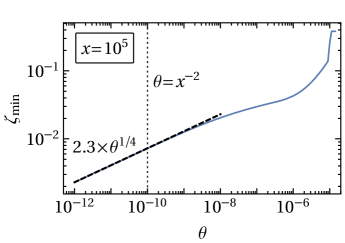
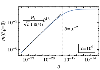
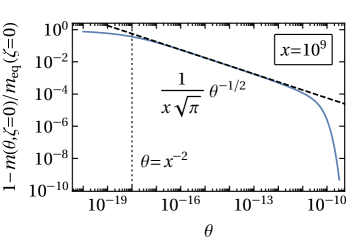
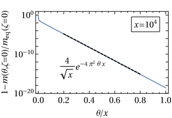
Figure 2: Time-evolution of an initially vanishing [Eq. 16] OP profile $\mathpzc{m}(\theta,\zeta)$, subject to the linearized model B dynamics [Eqs. 21 and 20] in the supercritical regime $x\gg 1$ [see Eq. 18b]. (a) $\mathpzc{m}(\theta,\zeta)$ as a function of $\zeta$ for rescaled times $\theta=10^{-8},10^{-6},10^{-5}$, and $\infty$ corresponding to the solid, dashed, dotted, and dashed-dotted curves, respectively. (b) Position $\zeta_{\text{min}}$ of the global minimum of the profile (within the left half $0\leq\zeta<1/2$ of the film) as a function of the rescaled time $\theta$. The dashed line indicates the prediction of Eq. 47, where the proportionality factor resulting from a fit is $\approx 2.3$ [Eq. 50]. (c) OP $\mathpzc{m}(\theta,\zeta=0)$ at the wall at early times $\theta\ll x^{-2}$. The dashed line indicates the asymptotic prediction given in Eq. 44. (d) OP $\mathpzc{m}(\theta,\zeta=0)$ at the wall at intermediate times, i.e., for $x^{-2}\ll\theta\ll x^{-1}$. The dashed line represents the intermediate asymptotic law in Eq. 53. (e) At late times $\theta\gtrsim x^{-1}$ the OP $\mathpzc{m}(\theta,\zeta=0)$ saturates exponentially. The dashed line indicates the asymptotic prediction given in Eq. 57. The dotted vertical lines in panels (b), (c), and (d) mark the approximate boundary between the early- and intermediate asymptotic regimes [see the discussion in Sec. IV.2 as well as Eq. 63 below]. The specific values of $x$ in the various panels are chosen for illustrative purposes, as being representative of the various behaviors of the system.

Here, we focus on the case of large reduced temperatures, $x\gg 1$, and study the associated asymptotic behavior of the OP dynamics, which is expected to differ from the one discussed in the preceding section. In Fig. 2(a), the time evolution of the profile for large $x$ is illustrated, based on the numerical Laplace inversion of Eq. 26. In order to proceed with the asymptotic analysis, we note that the time dependence of $\mathpzc{m}(\theta,\zeta)$ is essentially encoded in the dependence of $\lambda_{\pm}$ on $s$ [Eq. 25] and that, according to Eq. 33, the dominant contribution to $\mathpzc{m}(\theta,\zeta)$ stems from values of $|s|\sim 1/\theta$. For $x\gg 1$, one thus infers from Eq. 25 the occurrence of three characteristic regimes: (i) $|s|\gg x^{2}$, (ii) $x\ll|s|\ll x^{2}$, and (iii) $|s|\ll x$, which translate to an early-, intermediate-, and late-time asymptotic regime defined by (i) $\theta\ll x^{-2}$, (ii) $x^{-2}\ll\theta\ll x^{-1}$, and (iii) $\theta\gg x^{-1}$, respectively.

IV.2.1 Early-time asymptotic regime

The behavior of $\mathpzc{m}(\theta,\zeta=0)$ for $\theta\to 0$ can be inferred in Laplace space from studying the limit $s\to\infty$ . In this limit, Eqs. 25 and 26 reduce to the expressions in Eqs. 35 and 36, respectively. This implies that the short-time properties of the profile for any large but finite $x$ in fact obey the critical scaling discussed in Sec. IV.1. Accordingly, at early times, the OP $\mathpzc{m}(\theta,\zeta=0)$ at the wall increases as in Eq. 44, and the spatial behavior of the OP near the wall is described by Eqs. 47 and 49. This is confirmed by the plots in Figs. 2(b) and (c), where the position $\zeta_{\text{min}}$ of the global minimum of the OP within the range $0\leq\zeta<1/2$ and the time evolution of $\mathpzc{m}(\theta,\zeta=0)$, respectively, is illustrated for $x\gg 1$. As discussed above, for $x\gg 1$, the early-time regime (i) crosses over to the intermediate regime (ii) approximately at a time $\theta\sim x^{-2}$, which is indicated in Fig. 2 by dotted vertical lines.

IV.2.2 Intermediate asymptotic regime

For large $x\gg 1$, an intermediate asymptotic temporal regime is expected to arise for times $\theta$ such that $x^{-2}\ll\theta\ll x^{-1}$. In order to determine the behavior of $\mathpzc{m}(\theta,\zeta=0)$ within this regime, we expand the inner square root in Eq. 25 around $s=0$ up to leading order in $s/x^{2}$, i.e., $\sqrt{x^{2}-4s}\simeq x-2s/x+\mathcal{O}(s^{2}/x^{3})$, which gives

$$\lambda_{+}\simeq\sqrt{x-s/x}\simeq\sqrt{x}\left(1-\frac{s}{2x^{2}}\right),\qquad\lambda_{-}\simeq\sqrt{s/x}.$$ (51)

Inserting Eq. 51 into Eq. 26 and keeping only the dominant terms for $x\gg 1$ with $x\ll|s|\ll x^{2}$ yields, after Laplace inversion, the OP profile in the intermediate asymptotic regime:

$$\mathpzc{m}(\theta,\zeta)\big{|}_{x\gg 1}\simeq\frac{H_{1}}{\sqrt{x}}\Bigg{[}\exp(-\zeta\sqrt{x})-\frac{1}{x\sqrt{\pi\theta}}\exp\left(-\frac{\zeta^{2}}{4\theta x}\right)+\exp(-(1-\zeta)\sqrt{x})-\frac{1}{x\sqrt{\pi\theta}}\exp\left(-\frac{(\zeta-1)^{2}}{4\theta x}\right)\Bigg{]}.$$ (52)

The first and the third term on the r.h.s. render together the asymptotic equilibrium profile reported in Eq. 31. Accordingly, the approach of the OP at the wall toward its long-time value $\mathpzc{m}_{\text{eq}}(\zeta=0)$ is described by

$$\mathpzc{m}_{\text{eq}}(\zeta=0)-\mathpzc{m}(\theta,\zeta=0)\simeq\frac{H_{1}}{\sqrt{\pi}x^{3/2}}\theta^{-1/2},$$ (53)

which, as shown in Fig. 2(d), accurately describes the numerical Laplace inversion of Eq. 26 within the intermediate asymptotic regime. One recognizes the expression in Eq. 52 as the superposition of the two corresponding asymptotic profiles obtained in a half-space [see Eq. 104 in Appendix A]. Within the intermediate asymptotic regime, the position $\zeta_{\text{min}}$ of the global minimum of the profile in, e.g., the left half of the film ($0\leq\zeta<1/2$), effectively follows, as function of time, a logarithmic behavior [see Eq. 106]:

$$\zeta_{\text{min}}\simeq x^{-1/2}[\ln(x^{2}\theta)-1],\qquad\text{for}\qquad x^{-2}\ll\theta\ll x^{-1}.$$ (54)

IV.2.3 Late-time asymptotic regime

The late-time asymptotic regime pertaining to the case $x\gg 1$, arises for times $\theta\gg x^{-1}$, corresponding to $|s|\ll x$ in Laplace space. In order to determine the corresponding behavior of the OP, we proceed as in the preceding subsection and insert in Eq. 26 the expansion given in Eq. 51, keeping only the most relevant terms for $|s|\ll x$ and $x\gg 1$. In Laplace space, this way one obtains the asymptotic profile

$$\hat{\mathpzc}{m}(s\ll x,\zeta)\big{|}_{x\gg 1}\simeq\frac{2}{s\sqrt{x}}\exp\left(\frac{s}{4x^{3/2}}-\frac{\sqrt{x}}{2}\right)\cosh\left[\left(\frac{1}{2}-\zeta\right)\sqrt{x}\right]\\ -\frac{1}{\sqrt{s}x^{3/2}}\exp\left(\frac{s}{4x^{3/2}}\right)\cosh\left[\left(\frac{1}{2}-\zeta\right)\sqrt{\frac{s}{x}}\right]\big{/}\sinh\left(\frac{1}{2}\sqrt{\frac{s}{x}}\right).$$ (55)

Note that, except from a pole at $s=0$, this expression has a regular Laurent expansion in terms of $s$, with no branch cut. At the wall ($\zeta=0$), Eq. 55 reduces to $\hat{\mathpzc}{m}(s,\zeta=0)=\exp(s/(4x^{3/2}))x^{-1/2}\left[1/s-\coth(\sqrt{s/x}/2)/(\sqrt{s}x)\right]$. Using the series representation of $\coth$ in terms of simple fractions (see, e.g., §1.421 in Ref. Gradshteyn and Ryzhik (2014)), the Laplace inversion is obtained as

$$\begin{split}\mathpzc{m}(\theta\gg 1/x,\zeta=0)/H_{1}&\simeq\frac{1}{\sqrt{x}}-\frac{2}{x}-\frac{4}{x}\sum_{k=1}^{\infty}\exp\left[-4\pi^{2}k^{2}\left(\theta x+\frac{1}{4\sqrt{x}}\right)\right]\\ &=\frac{1}{\sqrt{x}}-\frac{4}{x}\vartheta_{3}\left(0,\,\exp\left[-4\pi^{2}\left(\theta x+\frac{1}{4\sqrt{x}}\right)\right]\right),\end{split}$$ (56)

where $\vartheta_{3}$ denotes the elliptic Jacobi theta function Olver et al. (2010). In the limit $\theta\to\infty$, the leading contribution to the sum is given by the term with $k=1$, such that

$$\mathpzc{m}(\theta\to\infty,\zeta=0)\simeq\frac{H_{1}}{\sqrt{x}}-\frac{4H_{1}}{x}\exp\left(-4\pi^{2}\theta x\right),\qquad\text{for}\qquad x\gg 1.$$ (57)

Accordingly, the equilibrium OP at the wall, $\mathpzc{m}_{\text{eq}}(\zeta=0)\simeq H_{1}/\sqrt{x}$ [see Eq. 30], is approached exponentially at late times. As shown in Fig. 2(e), Eq. 57 accurately matches the behavior of the OP determined numerically from the exact expression in Eq. 26. A numerical analysis reveals that Eq. 57 is, in fact, reliable for $x\gtrsim 10^{4}$.

IV.3 Behavior of the second derivative of the profile

IV.3.1 Critical quench ($x=0$)

For the purpose of analyzing the CCF (see Sec. VI below), it is useful to determine also the behavior of the second derivative of the OP profile $\mathpzc{m}(\theta,\zeta)$ at the boundary $\zeta=0$ (or, equivalently, at $\zeta=1$). Focusing first on a critical quench ($x=0$), Eq. 36 yields

$$\partial_{\zeta}^{2}\hat{m}(s,\zeta)\big{|}_{\zeta=0}=-\frac{H_{1}}{2\omega^{3}}\left[\coth(\omega/2)+\cot(\omega/2)\right]$$ (58)

for the Laplace transform of $\mathpzc{m}$. Proceeding as in Sec. IV.1.1, one finds

$$\partial_{\zeta}^{2}m(\theta,\zeta)\big{|}_{\zeta=0}\simeq\frac{H_{1}}{\sqrt{2}\ \Gamma(3/4)}\theta^{-1/4},\qquad\text{for}\qquad\theta\lesssim\theta^{*}_{e},$$ (59)

as the short-time asymptotic behavior . At late times $\theta\gtrsim\theta^{*}_{e}$, instead, $\partial_{\zeta}^{2}\mathpzc{m}$ approaches the equilibrium value [see Eq. 29]

$$\partial_{\zeta}^{2}\mathpzc{m}_{\text{eq}}(0)\big{|}_{x=0}=2H_{1}$$ (60)

exponentially.

IV.3.2 Off-critical quench ($x\gg 1$)

From Eq. 27 one obtains the late-time limit of $\partial_{\zeta}^{2}\mathpzc{m}$ for $x\gg 1$ as

$$\partial_{\zeta}^{2}\mathpzc{m}_{\text{eq}}(0)\simeq H_{1}\sqrt{x}.$$ (61)

Performing an analysis analogous to the one in Sec. IV.2 yields the following asymptotic behaviors of $\partial^{2}_{\zeta}\mathpzc{m}$ for $x\gg 1$ [49]:

$$\frac{H_{1}}{\sqrt{2}\ \Gamma(3/4)}\theta^{-1/4},\qquad \theta\ll x^{-2},$$ (62a)

$$\partial^{2}_{\zeta}\mathpzc{m}_{\text{eq}}(0)\left(1+\frac{1}{2\sqrt{\pi}x^{3}}\theta^{-3/2}\right), x^{-2}\ll\theta\ll x^{-1},$$ (62b)

$$\partial^{2}_{\zeta}\mathpzc{m}_{\text{eq}}(0)\left(1+\frac{16\pi^{2}}{x^{3/2}}e^{-4\pi^{2}x\theta}\right), \theta\gg x^{-1},$$ (62c)

where we note that $\partial^{2}_{\zeta}\mathpzc{m}_{\text{eq}}(0)|_{x\to\infty}\simeq H_{1}\sqrt{x}$.

IV.4 Summary

We have shown that, for $x\gtrsim 10^{2}$, the behavior of the OP at the wall, $\mathpzc{m}(\theta,\zeta=0)$, exhibits three characteristic regimes (see Sec. IV.2):

$$\frac{H_{1}}{\sqrt{2}\,\Gamma(5/4)}\theta^{1/4},\qquad \theta\ll x^{-2},$$ (63a)

$$\mathpzc{m}_{\text{eq}}(0)\left(1-\frac{1}{\sqrt{\pi}x}\theta^{-1/2}\right), x^{-2}\ll\theta\ll x^{-1},$$ (63b)

$$\mathpzc{m}_{\text{eq}}(0)\left(1-\frac{4}{\sqrt{x}}e^{-4\pi^{2}x\theta}\right), \theta\gg x^{-1},$$ (63c)

where we have used the relationship $\mathpzc{m}_{\text{eq}}(0)\simeq H_{1}/\sqrt{x}$ for $x\to\infty$ [see Eq. 30]. For $x\lesssim 10^{2}$, the intermediate asymptotic regime in Eq. 63b effectively disappears, leaving only the early- and late-time regimes, which are characteristic for a critical quench (see Sec. IV.1.1):

$$\frac{H_{1}}{\sqrt{2}\,\Gamma(5/4)}\theta^{1/4},\qquad \theta\ll\theta^{*}_{e},$$ (64a)

$$\mathpzc{m}_{\text{eq}}(0)\left(1-\frac{1}{\pi^{2}}e^{-16\pi^{4}\theta}\right), \theta\gg\theta^{*}_{e},$$ (64b)

where $\theta^{*}_{e}\simeq 10^{-4}$ [see Eq. 41].

At the time $\theta^{*}\in\{\theta^{*}_{e},x^{-2}\}$, at which the crossover from the early-time growth [Eq. 63a] to the saturation regime [Eqs. 63b and 63c] occurs, one typically has $\mathpzc{m}(\theta^{*},0)\simeq\mathpzc{m}_{\text{eq}}(0)$, i.e., the OP is almost fully equilibrated. Indeed, for $x\gg 1$, Eq. 30 gives $\mathpzc{m}_{\text{eq}}(0)\simeq H_{1}/\sqrt{x}$. Approximately at $\theta\sim x^{-2}$, i.e., at the end of the early-time regime, this value is reached by $\mathpzc{m}(\theta,\zeta=0)$ evolving according to Eq. 63a. For $x\ll 1$, correspondingly, the equilibrium value $\mathpzc{m}_{\text{eq}}(0)\simeq H_{1}/6$ predicted by Eq. 29 is reached at a time $\theta\simeq(\sqrt{2}\Gamma(5/4)/6)^{4}\simeq 2\times 10^{-3}$, which follows by equating $\mathpzc{m}_{\text{eq}}(0)$ with $\mathpzc{m}(\theta,0)$ in Eq. 64a and which is consistent with the estimate of $\theta^{*}_{e}$ in Eq. 41.

Notably, for large $x>0$, at the wall the OP $\mathpzc{m}$ attains equilibrium much earlier than far from the wall. Indeed, at the end of the early-time regime, i.e., at a time $\theta\simeq\theta^{*}\simeq x^{-2}$, the OP minimum has propagated only a distance $\zeta_{\text{min}}(\theta^{*})\sim x^{-1/2}\ll 1/2$ into the bulk [see Eqs. 50 and 2]. A numerical analysis of the full solution in Eq. 26 reveals that the two OP minima in the film (see Fig. 2) merge in its middle around a characteristic time

$$\theta_{\text{min}}^{*}\sim\min(x^{-1},\theta^{*}_{e}).$$ (65)

This time scale is close to that of the onset of the exponential saturation regime of the profile [see Eqs. 63c and 64b]. This regime is characteristic for a film, whereas the profile in a half-space only shows the algebraic growth and saturation behaviors reported in Eqs. 63a and 63b (see Appendix A as well as Ref. Diehl and Janssen (1992)). Accordingly, within the linear model B and for $(++)$ boundary conditions, the time $\theta^{*}_{\text{min}}$ in Eq. 65 can be understood as the typical time scale for the onset of the interaction between the two walls after a quench.

V Nonlinear quench dynamics

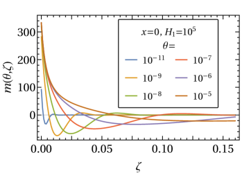
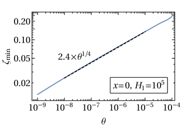
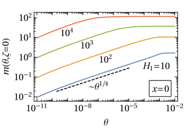
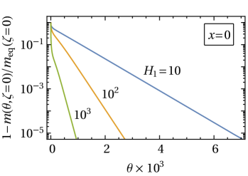
Figure 3: Time evolution, within the nonlinear model B [Eq. 19], of the OP profile at criticality ($x=0$) and for $H_{1}\gg 1$, starting from a flat, vanishing initial configuration [Eq. 16]. (a) Profile $\mathpzc{m}(\theta,\zeta)$ near one wall for various rescaled times $\theta$. (b) Position of the global minimum of $\mathpzc{m}(\theta,\zeta)$ as a function of time $\theta$; for all values of $H_{1}\gg 1$, $\zeta_{\text{min}}$ exhibits essentially the same behavior. (c) Increase of the OP at the wall $\mathpzc{m}(\theta,\zeta=0)$ for various values of $H_{1}$. The dashed line indicates the scaling behavior implied by Eq. 64a. (d) Relaxation of the OP at the wall to its equilibrium value $\mathpzc{m}_{\text{eq}}(\zeta=0)$. For large $H_{1}\gg 1$, an intermediate asymptotic law [Eq. 70] emerges. (e) For times $\theta\gtrsim\theta^{*}_{e}\simeq 10^{-4}$, the relaxation of the OP proceeds exponentially [see Eq. 71].

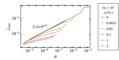
Figure 4: Evolution of the rescaled OP profile $\mathpzc{m}(\theta,\zeta)$ in a film within the nonlinear model B. (a) Temporal crossover of the OP at the boundary $\mathpzc{m}(\theta,\zeta=0)$ between the linear and the nonlinear intermediate asymptotic behavior, as characterized by the value of $x/H_{1}$. The dashed and the dotted lines represent the intermediate asymptotic laws given in Eqs. 63b and 70, respectively. (b) Position of the global minimum of $\mathpzc{m}(\theta,\zeta)$ as a function of time $\theta$ for large $H_{1}\gg 1$ and various values of $x/H_{1}$. The dashed line represents the asymptotic law in Eq. 67, identified from the numerical data. Due to the limited numerical resolution, the evolution of $\zeta_{\text{min}}$ could not be followed up to $\zeta=1/2$. However, a visual inspection of the profiles reveals that at the times at which the plotted curves end, the two minima of the film profile (corresponding to $\zeta_{\text{min}}$ and $1-\zeta_{\text{min}}$) have in fact merged.

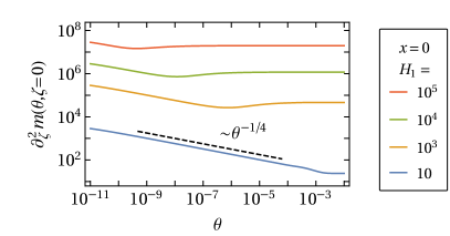
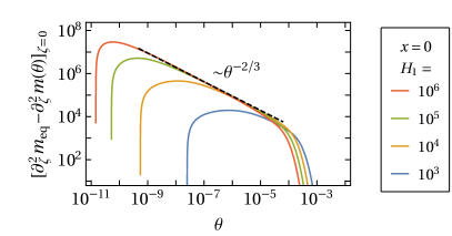
Figure 5: Behavior of $\partial^{2}_{\zeta}\mathpzc{m}$ as a function of time within the nonlinear model B for various strengths of the surface field $H_{1}$ and at criticality $x=0$. For small $H_{1}$, $\partial_{\zeta}^{2}\mathpzc{m}$ varies in accordance with Eq. 62a [dashed line in panel (a)], which follows from the linear model B. For large $H_{1}$, panel (b) shows that an intermediate asymptotic regime emerges, where $\partial_{\zeta}^{2}\mathpzc{m}$ approaches its equilibrium value algebraically, i.e., $[\partial_{\zeta}^{2}\mathpzc{m}]_{\zeta=0}\simeq[\partial_{\zeta}^{2}\mathpzc{m}_{\text{\,eq}}]_{\zeta=0}-C\theta^{-2/3}$, with $C\simeq 9$ as determined from a fit [see Eq. 73].

In this section, within MFT, we determine the dynamics of the fully nonlinear model B. This is carried out numerically by discretizing Eqs. 19 and 20 in terms of finite differences on a spatial grid and by integrating the resulting system of first-order ordinary differential equations in time Moin (2010). As before, a flat, vanishing profile [Eq. 16] is used as initial configuration .

Within the linearized model B, $H_{1}$ merely appears as an overall scaling factor of the profile $\mathpzc{m}(\theta,\zeta)$ [see Eq. 26]. The characteristic time scales are independent of $H_{1}$ [see Eqs. 63 and 64]. In contrast, the dynamics of the fully nonlinear model B [Eqs. 19 and 20] is expected to exhibit an interplay between $H_{1}$ and the scaling variable $x$. As shown in Ref. Gross et al. (2016), this applies already to the properties of the equilibrium profile. Specifically, for $x\geq 0$, MFT predicts the following equilibrium behavior of the OP value at the wall Gross et al. (2016):

$$H_{1}\left(\frac{1}{6}-\frac{x}{360}\right), H_{1}\lesssim 1,\,x\lesssim 1,$$ (66a)

$$\frac{H_{1}}{x^{1/2}}, H_{1}\lesssim x,\,x\gg 1,$$ (66b)

$$2^{1/4}H_{1}^{1/2}-\frac{x}{3\times 2^{1/4}H_{1}^{1/2}}, H_{1}^{1/2}\gg x,\,H_{1}\gg 1.$$ (66c)

Equations 66a and 66b in fact coincide with the results of linear MFT [see Eqs. 29 and 30], while Eq. 66c can be obtained from a short-distance expansion within nonlinear MFT (see Ref. Gross et al. (2016)). The ranges of validity of the asymptotic behaviors reported above result from a comparison between linear and nonlinear MFT. Notably, in the presence of a mass constraint, linear MFT remains a valid approximation for $H_{1}\lesssim 1$, even as $x\to 0$ Gross et al. (2016). For $H_{1}\gg 1$ and $x\ll H_{1}$, instead, linear MFT fails to accurately capture the equilibrium profile Gross et al. (2016). Accordingly, we expect the nonlinear term $\mathpzc{m}^{3}$ [see Eq. 19] to play also a role in the dynamics.

Figures 3 and 4 summarize the dynamics of the OP profile governed by the nonlinear model B for $(++)$ boundary conditions after a quench to criticality ($x=0$) and to a supercritical temperature ($x\gg 1$), respectively. As in the linear case (see Figs. 1 and 2), the increase of the OP at the wall is supported by transport of mass from the interior of the film, giving rise to a pronounced minimum of the profile moving towards the center. A numerical analysis, illustrated in Fig. 3, shows that this minimum follows a subdiffusive law:

$$\zeta_{\text{min}}\simeq 2.4\times\theta^{1/4}.$$ (67)

Except for the slightly larger value of the prefactor , this relation is identical to the one obtained within the linear model B [see Eq. 50]. Panels (c)–(e) of Fig. 3 illustrate the increase of the OP at the wall, $\mathpzc{m}(\theta,\zeta=0)$. For large $H_{1}$ one can identify three asymptotic regimes: in addition to the initial algebraic growth $\mathpzc{m}(\theta,0)\propto\theta^{1/4}$ [Fig. 3(c)] and the late-time exponential saturation [Fig. 3(e)], an intermediate asymptotic regime emerges for $H_{1}\gg 1$, in which the OP saturates algebraically. For $x=0$, the latter regime is not present in linear MFT [see Eqs. 64 and 1]. Below, these various regimes are analyzed further.

The effect of a nonzero reduced temperature $x>0$ on the OP dynamics is illustrated in Fig. 4. As shown in panel (a), upon increasing $x$, the intermediate asymptotic law identified in Fig. 3(d) crosses over from a behavior dominated by the nonlinearity towards that of the linear model B reported in Eq. 63b. At late times, the OP at the wall $\mathpzc{m}(\theta,\zeta=0)$ always saturates exponentially. Figure 4(b) shows that, upon increasing $x$ at fixed $H_{1}\gg 1$, the dynamics of the OP minimum significantly deviates from Eq. 67, which holds at criticality $x=0$. Due to limited numerical accuracy, for large $x$ the evolution of $\zeta_{\text{min}}$ cannot be followed up to values of $\zeta_{\text{min}}\sim\mathcal{O}(1)$. However, an inspection of the actual profile $\mathpzc{m}(\theta,\zeta)$ reveals that, at a time around $\theta\sim x^{-1}$, the two minima in the film profile have merged at the center of the system and the profile has essentially reached equilibrium. Accordingly, we conclude that, also for the nonlinear model B, the characteristic time scale for the onset of the interaction between the two walls is given by Eq. 65.

We now return to a quantitative discussion of the OP dynamics at the wall, i.e., of $\mathpzc{m}(\theta,\zeta=0)$, within the nonlinear model B. The asymptotic behavior can be analyzed based on the relative weight of the individual terms on the r.h.s. of Eq. 19, i.e., $-\partial_{\zeta}^{2}\mathpzc{m}+x\mathpzc{m}+\mathpzc{m}^{3}$. We emphasize that the term $\partial_{\zeta}^{2}\mathpzc{m}$ is always relevant, because it is responsible for the emergence of the nontrivial equilibrium profile $\mathpzc{m}_{\text{eq}}$ (see also Ref. Gross et al. (2016)). In fact, it provides the driving force for the evolution of the profile away from the flat initial configuration. The analysis of the asymptotic dynamics is facilitated by the knowledge of the linear mean-field solutions reported in Sec. IV.

At sufficiently early times $\theta\ll 1$, $\mathpzc{m}$ is small owing to the initial condition in Eq. 16. Consequently, $x\mathpzc{m}$ and $\mathpzc{m}^{3}$ are negligible and the behavior reported in Eqs. 59 and 63a applies, which is solely driven by the term $\partial_{\zeta}^{2}\mathpzc{m}$ on the r.h.s. of Eq. 19. In the course of the early-time dynamics given in Eqs. 63a and 59, the term $x\mathpzc{m}$ increases and it becomes comparable to $\partial_{\zeta}^{2}\mathpzc{m}$ around the time

$$\theta^{*}_{x}\sim x^{-2},$$ (68)

while $\partial_{\zeta}^{2}\mathpzc{m}$ becomes comparable to $\mathpzc{m}^{3}$ around the time

$$\theta^{*}_{3}\sim H_{1}^{-2}.$$ (69)

The relative magnitude of $\theta^{*}_{x}$ and $\theta^{*}_{3}$ plays a central role in characterizing the deviation of the time evolution from the linear mean-field behavior, as it is analyzed in the following.

Case $H_{1}\ll x$, $x\gtrsim 100$: Since in this case $\theta^{*}_{x}\ll\theta^{*}_{3}$, the evolution of $\mathpzc{m}(\theta,0)$ crosses over at $\theta\sim\theta^{*}_{x}$ from the behavior described in Eq. 63a to the intermediate asymptotic regime of linear MFT reported in Eq. 63b, which requires $x\gtrsim 100$. According to Eqs. 63a and 66b, one has $\mathpzc{m}(\theta^{*}_{x},0)\simeq 0.78\times\mathpzc{m}_{\text{eq}}(0)$ at the time $\theta^{*}_{x}$. Since, in addition, $\mathpzc{m}_{\text{eq}}^{3}/(x\mathpzc{m}_{\text{eq}})\sim H_{1}^{2}/x^{2}\ll 1$, we conclude that in the present case, the term $\mathpzc{m}^{3}$ never exceeds $x\mathpzc{m}$. Accordingly, the time evolution for $\theta\gtrsim\theta^{*}_{x}$ closely follows the behavior of the linear model B given in Eq. 63. A numerical analysis confirms that, as expected from Eq. 63c, the crossover to the final exponential saturation regime occurs at a time $\theta^{*}_{e}\sim x^{-1}$. This crossover corresponds to the point of maximum curvature of the curves plotted in Fig. 4.

Case $H_{1}\ll x,x\lesssim 100$: For $x\lesssim 100$, the early-time regime, which is described by the linear model B behavior in Eq. 63a, proceeds up to the time $\theta^{*}_{e}\simeq 10^{-4}$ [Eq. 41], at which $\mathpzc{m}(\theta^{*}_{e},0)\simeq 0.48\times\mathpzc{m}_{\text{eq}}(0)$ [see Eq. 66a]. Since $\mathpzc{m}_{\text{eq}}^{3}/(x\mathpzc{m}_{\text{eq}})\sim H_{1}^{2}/(36x)\ll 1$, the dynamics is governed by the linear model B also for $\theta>\theta^{*}_{e}$, where $\mathpzc{m}(\theta,0)$ follows the exponential saturation law reported in Eq. 63c.

Case $H_{1}\gg x$, $H_{1}\gtrsim 100$: In this case one has $\theta^{*}_{3}\ll\theta^{*}_{x}$ (and $\theta^{*}_{3}\lesssim 10^{-4}$), such that the initial algebraic growth law in Eq. 63a is expected to cross over at $\theta\sim\theta^{*}_{3}$ to a different behavior characteristic of nonlinear dynamics. A numerical analysis, which is illustrated in Fig. 3 for $x=0$, reveals an effective intermediate asymptotic behavior of the form

$$\mathpzc{m}(\theta\gtrsim\theta^{*}_{3},0)\simeq\mathpzc{m}_{\text{eq}}(0)\left(1-C\theta^{-2/3}\right),\qquad\text{with}\qquad C\simeq 0.2\times H_{1}^{-1.2},$$ (70)

where the dependence of $C$ on $H_{1}$ as well as the value of the exponent of $\theta$ have been determined from a fit of the numerical data. Using Eq. 66c, one obtains $\mathpzc{m}(\theta^{*}_{3},0)\simeq 0.66\times\mathpzc{m}_{\text{eq}}(0)$ and furthermore $\mathpzc{m}^{3}_{\text{eq}}/(x\mathpzc{m}_{\text{eq}})\sim 2^{1/2}H_{1}/x\gg 1$, indicating that the linear term $x\mathpzc{m}$ remains negligible compared to $\mathpzc{m}^{3}$ for times $\theta\gtrsim\theta^{*}_{3}$. Accordingly, no further intermediate asymptotic law is expected in this case. Instead, we find that, at a time $\theta^{*}_{e}\gg\theta^{*}_{3}$, the dynamics crosses over to a final exponential saturation regime,

$$\mathpzc{m}(\theta\gtrsim\theta^{*}_{e},0)\simeq\mathpzc{m}_{\text{eq}}(0)\left(1-\tilde{C}e^{-\tilde{A}\theta}\right),$$ (71)

which is illustrated in Fig. 3 for $x=0$. The parameters $\tilde{A}$ and $\tilde{C}$ are numerically found to depend on $H_{1}$ and $x$ in a way which does not lend itself to a meaningful fit based on the presently available data. As one infers from Fig. 3, for $x=0$ and for the considered values of $H_{1}$, the crossover time $\theta^{*}_{e}$ depends only weakly on $H_{1}$ and it can be estimated as

$$\theta^{*}_{e}\simeq 10^{-4},$$ (72)

which agrees with Eq. 41. For $x\gg 1$, instead, a numerical analysis (data not shown) indicates that the crossover time is approximately given by $\theta^{*}_{e}\sim x^{-1}$, which is the same scaling law as in Eq. 63c. Equations 70 and 71 replace the intermediate and late-time asymptotics in Eq. 63 in the nonlinear case.

Case $H_{1}\gg x$, $H_{1}\lesssim 100$: In this case one has $\theta^{*}_{3}\gtrsim\theta^{*}_{e}$, such that, according to Eq. 64, before the nonlinearity becomes relevant, the dynamics crosses over from the early-time growth to an exponential saturation regime at a time $\theta\simeq\theta^{*}_{e}$. A numerical analysis reveals that this exponential saturation in fact persists until equilibrium is reached. The irrelevance of the nonlinear term is consistent with the fact that, in this case, static linear MFT accurately approximates $\mathpzc{m}_{\text{eq}}$ [see Eq. 66a].

In Fig. 5, the temporal evolution of the second derivative of the profile at the wall, $\partial^{2}_{\zeta}\mathpzc{m}(\theta,\zeta)|_{\zeta=0}$, is illustrated for $x=0$ and for various values of the surface field $H_{1}$. For times $\theta\lesssim\theta^{*}_{3}$ [Eq. 69], $\partial_{\zeta}^{2}\mathpzc{m}$ generally evolves following the predictions of the linear model B [see Eq. 62a]. For large values of $H_{1}\gg 1$ and for $x\ll H_{1}$, the nonlinear term becomes relevant and causes the appearance of an intermediate asymptotic saturation regime of the form [see Fig. 5(b)]

$$\partial_{\zeta}^{2}\mathpzc{m}|_{\zeta=0}\simeq\partial_{\zeta}^{2}\mathpzc{m}_{\text{eq}}|_{\zeta=0}-C\theta^{-2/3},\qquad\text{for}\qquad\theta^{*}_{3}\ll\theta\ll\theta^{*}_{e},$$ (73)

where $C\simeq 9$ follows together with the value of the exponent of $\theta$ from a fit to the numerical data, while $\theta_{e}^{*}$ coincides with Eq. 72.

In conclusion, except for the case $H_{1}\gg x$, $H_{1}\gtrsim 100$, the expressions in Eqs. 63 and 64, based on the linearized dynamics, generally provide an accurate description of the asymptotic dynamics of the nonlinear model B.

VI Critical Casimir force

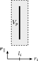
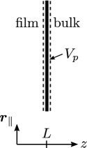
Figure 6: (a) The generalized force $K_{i}$, which is acting along the coordinate direction $r_{i}$ ($i\in\{x,y,z\}$) onto a plate of finite extent (thin black rectangle), is obtained via an integration of the derivative of the Hamiltonian density over an arbitrary enclosing volume $V_{p}$ [shaded rectangle; see Eq. 76]. This plate of transverse area $A$ is located at $r_{i}=l_{i}$ and lies in the plane spanned by the lateral coordinates $\mathbf{r}_{\parallel}=\sum_{j\in\{x,y,z\}\backslash i}r_{j}\mathbf{e}_{j}$. (b) Here, the plate represents one of the two boundaries between the film and the surrounding bulk system. Along the lateral directions, both the plate and the volume $V_{p}$ are infinitely extended. The force acting on the plate can be interpreted as the CCF [see Eq. 81], which is determined by shifting the surfaces of $V_{p}$ (dashed lines) directly next to the corresponding surfaces of the plate.

Following Ref. Dean and Gopinathan (2010), in this section we obtain the dynamic CCF based on the notion of a generalized force associated with the interaction between the OP field $\phi$ and the boundary. In order to recall the corresponding formalism, we first consider an arbitrary volume $V$ containing a single plate with finite transverse area [see Fig. 6(a)] and subsequently show how this approach renders the CCF in a film. For simplicity, we assume the plate to be perpendicular to the coordinate axis $i\in\{x,y,z\}$ and to be located at the position $r_{i}=l_{i}$. The OP $\phi$ gives rise to the free energy functional

$$\mathcal{F}=\int_{V}\mathrm{d}^{d}r\left\{\mathcal{H}_{0}(\phi(\mathbf{r}),\nabla\phi(\mathbf{r}))+\mathcal{U}_{p}(l_{i},\phi(\mathbf{r}))\right\}\equiv\int_{V}\mathrm{d}^{d}r\,\mathcal{H}(l_{i},\phi(\mathbf{r}),\nabla\phi(\mathbf{r})),$$ (74)

where $\mathcal{H}=\mathcal{H}_{0}+\mathcal{U}_{p}$, $\mathcal{H}_{0}$ is an arbitrary bulk Hamiltonian density (energy per volume), and the boundary potential

$$\mathcal{U}_{p}(l_{i},\phi)=\delta(r_{i}-l_{i})U_{p}(\phi)$$ (75)

accounts for the interaction with strength $U_{p}(\phi)$ between the plate and the OP field. (Note that, in contrast to Eq. 9, here $\mathcal{F}$ is defined not per unit area and per $k_{B}T$.) According to the principle of virtual work, for any configuration of $\phi$ the generalized force $K_{i}$ acting on the plate is given by Dean and Gopinathan (2010)

$$K_{i}\equiv-\frac{\partial\mathcal{F}}{\partial l_{i}}=\int_{V_{p}}\mathrm{d}^{d}r\frac{\partial\,\mathcal{U}_{p}(l_{i},\phi)}{\partial l_{i}}=\int_{V_{p}}\mathrm{d}^{d}r\frac{\partial\,\mathcal{H}(l_{i},\phi,\nabla\phi)}{\partial l_{i}},$$ (76)

where $V_{p}$ is an arbitrary volume enclosing the plate as sketched in Fig. 6(a). The last two expressions in Eq. 76 follow from the spatially localized nature of the interaction $\mathcal{U}_{p}$, i.e., from the finite extent of the surface. Note that $K_{i}$ depends only on the static free energy functional and is therefore independent of the actual dynamics or conservation laws. Introducing the bulk chemical potential associated with $\mathcal{F}$ [see Eq. 14],

$$\mu\equiv\frac{\delta\mathcal{F}}{\delta\phi}=\frac{\partial\mathcal{H}}{\partial\phi}-\nabla_{j}\left(\frac{\partial\mathcal{H}}{\partial\nabla_{j}\phi}\right),$$ (77)

$K_{i}$ can, after some algebra, be expressed as

$$\begin{split}K_{i}&=-\int_{V_{p}}\mathrm{d}^{d}r\,\nabla_{j}\mathcal{T}_{ij}-\int_{V_{p}}\mathrm{d}^{d}r\mu\nabla_{i}\phi\\ &=-\int_{\partial V_{p}}\mathrm{d}^{d-1}s_{j}\,\left(\mathcal{T}_{ij}+\mu\phi\delta_{ij}\right)+\int_{V_{p}}\mathrm{d}^{d}r\,(\nabla_{i}\mu)\phi,\end{split}$$ (78)

in terms of the standard stress tensor

$$\mathcal{T}_{ij}=\frac{\partial\mathcal{H}}{\partial\nabla_{i}\phi}\nabla_{j}\phi-\delta_{ij}\mathcal{H},$$ (79)

where, in the previous expressions, summing over repeated indices is understood and $\partial V_{p}$ denotes the boundaries of $V_{p}$.

We now apply this formalism to a film, i.e., a volume bounded by two infinitely extended plates located at $l_{z}=0$ and $l_{z}=L$. At each plate, the volume $V_{p}$ is chosen such that its surfaces are located directly next to the corresponding surfaces of the plate, as sketched in Fig. 6(b). We define the CCF $\mathcal{K}$ as the generalized force [Eq. 76] per area $A$ acting on the boundary,

$$\mathcal{K}\equiv K_{z}/A,$$ (80)

in the limit $A\to\infty$. We describe the location of the right and the left boundary as $l_{z}=L/2\pm\tilde{l}_{z}$, respectively, and compute the derivative in Eq. 76 with respect to $\tilde{l}_{z}$, which ensures that at each boundary a variation $\mathrm{d}\tilde{l}_{z}>0$ increases the film thickness. Accordingly, Eq. 76 turns into $K_{z}=\mp\partial\mathcal{F}/\partial\tilde{l}_{z}$ at the right and the left boundary, respectively. Consistently with Eq. 7, the resulting CCF is therefore repulsive if the film free energy decreases upon increasing the film thickness. Owing to the no-flux boundary conditions [Eq. 15], the last term in the second equation of Eq. 78 vanishes for this choice of $V_{p}$. Upon taking into account the direction of the surface normals, the CCF finally follows from Eq. 78 as

$$\mathcal{K}=\bar{\mathcal{T}}_{zz}\big{|}_{z=0,L}-\bar{\mathcal{T}}_{zz,b}\>,$$ (81)

where

$$\bar{\mathcal{T}}_{ij}\equiv\mathcal{T}_{ij}+\mu\phi\delta_{ij}=\frac{\partial\mathcal{H}}{\partial\nabla_{i}\phi}\nabla_{j}\phi-\delta_{ij}(\mathcal{H}-\mu\phi),$$ (82)

and $\bar{\mathcal{T}}_{ij,b}$ denotes the corresponding expression of $\bar{\mathcal{T}}_{ij}$ in the bulk (where, within MFT, gradient terms are absent). Note that Eq. 81 has to be evaluated for the actual time-dependent solution $\phi(t,z)$ of the model B equations [Eq. 13].

Henceforth we shall call $\bar{\mathcal{T}}_{ij}$ the dynamical stress tensor . Remarkably, Eqs. 81 and 82 coincide with the formal expressions for the equilibrium CCF and the equilibrium stress tensor in the canonical ensemble, respectively, as derived in Ref. Gross et al. (2016). The dynamical stress tensor $\bar{\mathcal{T}}_{ij}$ differs from the standard equilibrium stress tensor $\mathcal{T}_{ij}$ used in the grand canonical ensemble Krech (1994) by the term $\mu\phi\delta_{ij}$ involving the chemical potential [Eqs. 14 and 77]. In fact, in an unconstrained (grand canonical) equilibrium, $\mu=\delta\mathcal{F}/\delta\phi=0$, such that in this case $\bar{\mathcal{T}}_{ij}=\mathcal{T}_{ij}$. However, in nonequilibrium, one generally has $\mu\phi\neq 0$, independently of the presence of a global or a local OP conservation law (see also Ref. Dean and Gopinathan (2010)). For the Landau-Ginzburg free energy functional considered in Eqs. 9 and 10, one has

$$\bar{\mathcal{T}}_{zz}=\frac{1}{2}(\partial_{z}\phi)^{2}+\frac{1}{2}r\phi^{2}+\frac{1}{8}g\phi^{4}-\phi\partial_{z}^{2}\phi.$$ (83)

In Ref. Krüger et al. (2018), a related nonequilibrium stress formulation has been analyzed for fluids far from criticality .

In order to proceed, we recall that the film is taken to have a vanishing mass [see Eq. 17]. In accordance with Ref. Gross et al. (2016), we therefore also assume that the bulk medium surrounding the film has a vanishing mean OP:

$$\phi_{b}=0.$$ (84)

Consequently, the associated bulk pressure $p_{b}=\bar{\mathcal{T}}_{zz,b}=0$ vanishes, too. Upon introducing the MFT scaling variables defined in Eq. 6, Eq. 81 [taking into account Eq. 84] can be brought into the scaling form given in Eq. 8:

$$\mathcal{K}=L^{-4}\Delta_{0}\left[\frac{1}{2}(\partial_{\zeta}\mathpzc{m})^{2}+\frac{1}{2}x\mathpzc{m}^{2}+\frac{3}{4}\mathpzc{m}^{4}-\mathpzc{m}\partial_{\zeta}^{2}\mathpzc{m}\right]_{\zeta=0,1},$$ (85)

where

$$\Delta_{0}=\frac{6}{g}=(\phi_{t}^{(0)}\xi_{+}^{(0)})^{2}$$ (86)

represents a mean-field amplitude, which can be expressed in terms of the non-universal critical amplitudes $\phi_{t}^{(0)}$ and $\xi_{+}^{(0)}$ defined in Eqs. 5 and 6. Consequently, the expression multiplying $L^{-4}$ on the r.h.s. of Eq. 85 represents the suitably normalized scaling function $\Xi(\theta,x,H_{1})$ of the CCF. A ratio of observables independent of $\Delta_{0}$ is provided by $\mathcal{K}/\mathcal{K}_{\text{eq}}$, where $\mathcal{K}_{\text{eq}}\equiv\mathcal{K}|_{t\to\infty}$ denotes the equilibrium CCF.

VI.1 Critical Casimir forces within linear mean field theory

Here, we analyze the dynamics of the CCF [Eq. 81] emerging within the linear model B, using a flat profile [Eq. 16] as initial condition. Accordingly, the CCF is completely determined by the expression of the profile given in Eq. 26. Due to the boundary conditions in Eq. 20a, the first term in the square brackets in Eq. 81 is constant and equal to $H_{1}^{2}/2$. Therefore the scaling function $\Xi$ of the CCF [see Eqs. 8, 81, 85, and 86 reduces to

$$\Xi/\Delta_{0}=\frac{1}{2}H_{1}^{2}+\frac{1}{2}x\mathpzc{m}^{2}-\mathpzc{m}\partial_{\zeta}^{2}\mathpzc{m}.$$ (87)

Note that, within the linear model B, $\Xi\propto H_{1}^{2}$, because $H_{1}$ enters the profile $\mathpzc{m}$ as an overall prefactor [see Eq. 26].

VI.1.1 Critical quench ($x=0$)

According to Eqs. 64 and 59, at early times one has

$$\mathpzc{m}\partial_{\zeta}^{2}\mathpzc{m}\simeq\frac{\sqrt{2}}{\pi}H_{1}^{2},\qquad\theta\lesssim\theta^{*}_{e}.$$ (88)

This implies that, correspondingly, the CCF in Eq. 87 attains a non-vanishing value:

$$\Xi(\theta\lesssim\theta^{*}_{e},x=0,H_{1})/\Delta_{0}\simeq\left(\frac{1}{2}-\frac{\sqrt{2}}{\pi}\right)H_{1}^{2}>0.$$ (89)

At late times ($\theta\to\infty$), instead, by using Eq. 29, we recover the equilibrium CCF at criticality in the canonical ensemble (see Ref. Gross et al. (2016)):

$$\Xi_{\text{eq}}(x=0,H_{1})\equiv\Xi(\theta\to\infty,x=0,H_{1})=\frac{1}{6}H_{1}^{2}\Delta_{0}.$$ (90)

The CCF scaling function $\Xi(\theta,x=0,H_{1})$ at criticality is illustrated as a function of time in Fig. 7. Interestingly, the CCF shows a non-monotonic transient behavior which interpolates between the early- and the late-time behaviors indicated above.

VI.1.2 Non-critical quench ($x\neq 0$)

From Eqs. 63 and 62 one concludes that, for $x\gg 1$, the early-time behavior in Eq. 89 applies to times $\theta\ll x^{-2}$. For $\theta\to\infty$, instead, the equilibrium value of the CCF Gross et al. (2016),

$$\Xi_{\text{eq}}(x\gg 1,H_{1})\equiv\Xi(\theta\to\infty,x\gg 1,H_{1})\simeq\frac{2H_{1}^{2}}{x}\Delta_{0},$$ (91)

is recovered. The non-equilibrium CCF for $x>0$ is generally weaker than that at criticality [see Fig. 7(a)], while one observes that, according to Eqs. 89 and 91, for $x\gg 1$ the magnitude of the CCF generally decreases with time. In the same limit but at intermediate times $\theta$ with $x^{-2}\lesssim\theta\lesssim x^{-1}$, the CCF decays as $\Xi\simeq(2\pi x^{2}\theta)^{-1}$ [see Fig. 7(b)]. This asymptotic expression follows upon inserting the corresponding expressions for $\mathpzc{m}$ [Eq. 63b] and $\partial_{\zeta}^{2}\mathpzc{m}$ [Eq. 62b] into Eq. 87 and by identifying the dominant term in the result. For times $\theta\gtrsim x^{-1}$ the CCF relaxes exponentially towards its equilibrium value (not shown).

In summary, within the linear model B and far from criticality (i.e., $x\gg 1$) the scaling function of the CCF exhibits the following asymptotic behavior:

$$\frac{1}{2}-\frac{\sqrt{2}}{\pi},\qquad \theta\ll x^{-2},$$ (92a)

$$\frac{1}{2\pi x^{2}}\theta^{-1}, x^{-2}\ll\theta\ll x^{-1},$$ (92b)

$$\frac{2}{x}, \theta\gg x^{-1}.$$ (92c)

For $0\leq x\,\lesssim\mathcal{O}(1)$, instead, the critical early- and late-time expressions given in Eqs. 89 and 90 apply, which occur for times $\theta\lesssim 10^{-4}$ and $\theta\gtrsim 10^{-2}$, respectively.

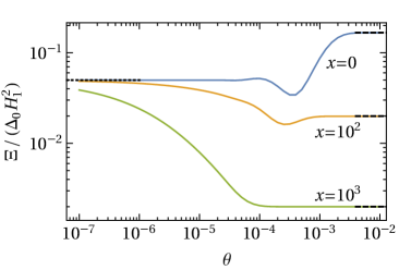
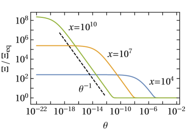
Figure 7: Scaling function $\Xi$ of the CCF as a function of time $\theta$ within the linear model B and for various values of the rescaled temperature $x$. In (a), the scaling function $\Xi$ is normalized by $\Delta_{0}H_{1}^{2}$, which is a common prefactor arising within linear MFT and which can be expressed in terms of physically accessible quantities [see Eqs. 86 and 6c and the related discussions]. The dotted and dashed lines represent the early- and late-time (equilibrium) values of the CCF reported in Eqs. 89, 90, and 91. In (b), instead, $\Xi$ is normalized by its late-time, equilibrium value. For large $x\gg 1$, the CCF follows an intermediate asymptotic behavior $\Xi\propto\theta^{-1}$ [Eq. 92b; dashed line in (b)]. At late times the scaling functions smoothly attain the value 1.

VI.2 Critical Casimir force within nonlinear mean field theory

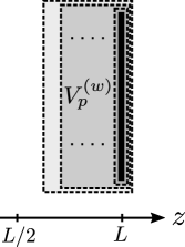
Figure 8: Illustration of the method used for determining numerically the CCF within the nonlinear model B. In order to minimize numerical errors, the CCF is calculated as an average over various integration volumes $V_{p}^{(w)}$ [see Eq. 94], which, starting from the outer one, progressively shrink towards the confining surface, as indicated by the dots in the figure. The left surface of $V_{p}^{(w)}$ is located at $z=w$ with $L/2<w<L$.

For the nonlinear model B, the time-dependent OP profile required to evaluate the CCF is determined numerically based on a finite-difference approximation of the dynamical equations as described in Sec. V. However, this approach can lead to numerical inaccuracies whenever the gradient of the OP profile is large, which is typically the case near a wall. In order to reduce the influence of this source of error for the CCF, we evaluate the latter by using the freedom in the choice of the integration volume $V_{p}$ [see Ref. Dean and Gopinathan (2010) and Eq. 76]. Specifically, we consider a volume $V_{p}^{(w)}$ enclosing the right plate which has a surface within the film at position $z=w$ with $L/2<w<L$ (see Fig. 8). Since this surface is not infinitesimally close to the plate, the second term in in the second equation of Eq. 78 does not vanish and the generalized force (per area) is given by

$$\mathcal{K}(w)=\bar{\mathcal{T}}_{zz}\big{|}_{z=w}-\bar{\mathcal{T}}_{zz,b}+\int_{w}^{L-\epsilon}\mathrm{d}z^{\prime}\,\phi(z^{\prime})\partial_{z^{\prime}}\mu(z^{\prime}).$$ (93)

Here, $\epsilon$ is an infinitesimal quantity which ensures that the integration ends just next to the inner surface of the boundary, noting that next to the outer boundary (i.e., in the bulk) the corresponding contribution would vanish owing to no-flux boundary conditions. The CCF (which is taken per area), being actually independent of $w$, can be conveniently obtained from Eq. 93 as an average over all possible locations $w$ between $L/2$ and $L$ :

$$\begin{split}\mathcal{K}=\frac{1}{L/2}\int_{L/2}^{L-\epsilon}\mathrm{d}w\,\mathcal{K}(w)&=\frac{1}{L/2}\int_{L/2}^{L-\epsilon}\mathrm{d}w\,\left[\bar{\mathcal{T}}_{zz}\big{|}_{z=w}+\int_{w}^{L-\epsilon}\mathrm{d}z^{\prime}\,\phi(z^{\prime})\partial_{z^{\prime}}\mu(z^{\prime})\right]-\bar{\mathcal{T}}_{zz,b}\\ &=\frac{2}{L}\int_{L/2}^{L-\epsilon}\mathrm{d}w\,\left[\bar{\mathcal{T}}_{zz}\big{|}_{z=w}+\left(w-\frac{L}{2}\right)\phi(w)\partial_{w}\mu(w)\right]-\bar{\mathcal{T}}_{zz,b}.\end{split}$$ (94)

We have checked numerically that this procedure renders the equilibrium value of the CCF reported in Eqs. 90 and 91 as well as in Ref. Gross et al. (2016).

In Fig. 9, the CCF obtained from Eq. 94 is shown as a function of time at criticality ($x=0$) for various values of the surface field $H_{1}$. According to the analysis in Sec. V, for $x=0$ the dynamics of the profile is governed by the linear model B for times $\theta\lesssim\theta^{*}_{3}\sim H_{1}^{-2}$ [Eq. 69]. This applies also to the CCF, which, in this regime, follows the prediction given in Eq. 89 (black dots in Fig. 9). Conversely, at times $\theta\gtrsim 100\times\theta^{*}_{e}\simeq 10^{-2}$, the CCF has essentially reached its equilibrium value, given by (see Eq. 90 and Ref. Gross et al. (2016))

$$\frac{1}{6}H_{1}^{2},\qquad H_{1}\ll 100,$$ (95a)

$$1.5\times(\ln H_{1})^{4}, H_{1}\gg 100.$$ (95b)

We recall that the monotonic increase of $\Xi_{\text{eq}}$ upon increasing $H_{1}$ in Eq. 95b is a consequence of the conserved mass in the film [Eq. 17] and of the fact that $\mathpzc{m}_{\text{eq}}(\zeta\to 0)\sim\zeta^{-1}$ within the nonlinear MFT (see Ref. Gross et al. (2016)). For large $H_{1}\gg 1$, the dynamics of the profile is affected by the nonlinear term (see Sec. V), which is reflected in the CCF by the emergence of a characteristic intermediate asymptotic regime occurring for times $\theta^{*}_{3}\lesssim\theta\lesssim\theta^{*}_{e}$ (see Fig. 9). A numerical analysis reveals that, within this regime, the CCF follows an algebraic decay, $\Xi\propto\theta^{-n}$, with an effective exponent $n\simeq 0.8$ (dashed line in Fig. 9).

It was shown in Ref. Gross et al. (2016) that, as a consequence of the mass constraint, the equilibrium CCF in the canonical ensemble is repulsive for $(++)$ boundary conditions. Here, we find that this repulsive character applies also to the non-equilibrium CCF over the whole time evolution.

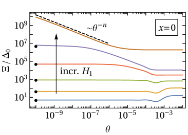
Figure 9: Dynamical CCF [Eq. 81] within the nonlinear model B, computed according to Eq. 94. The values of the surface field $H_{1}$ are (from bottom to top) $H_{1}=10,30,130,10^{3},10^{4}$, and $10^{6}$. The black dots correspond to the values of $\Xi$ at early times [Eq. 89], which are determined by the linear MFT. The dashed line indicates an algebraic behavior with an effective exponent $n\simeq 0.8$.

VII Summary and Outlook

In the present study, we have investigated the dynamics of the order parameter (OP) and of the critical Casimir force (CCF) in a fluid film after an instantaneous quench from a homogeneous high-temperature phase to a (rescaled) near-critical temperature $x$ [Eq. 6b]. The dynamics of the medium is taken to be described by model B within mean field theory, i.e., by a diffusive transport equation without noise. Initially, the OP profile $\mathpzc{m}(\theta=0,\zeta)=0$ vanishes across the film [Eqs. 5, 6d, and 6a]. The driving force for the dynamics stems from the presence of symmetric surface fields, which, in the long-time limit $\theta\to\infty$, give rise to an inhomogeneous OP profile across the film characteristic of critical adsorption with $(++)$ boundary conditions. The model B dynamics is supplemented by no-flux boundary conditions acting at the boundaries of the film, such that the total integrated OP within the film is constant at all times: $\int_{0}^{1}\mathrm{d}\zeta\,\mathpzc{m}(\theta,\zeta)=0$. Accordingly, the model used here realizes the canonical ensemble—the equilibrium, time-independent properties of which have been previously studied in Ref. Gross et al. (2016) and have been shown to lead to pronounced differences in the behavior of the CCF compared to the usual grand canonical ensemble. The analytical solution of the linearized model B is supplemented by a numerical solution of the full nonlinear model B equations. Our main findings are summarized as follows:

1. For small values of the surface field $H_{1}\lesssim 100$ [Eq. 6c] as well as for large rescaled temperatures $x\gg H_{1}$, the linear model B provides an accurate description of the full mean field dynamics of the OP in the film.

2. Both at criticality ($x=0$) and away from it ($x\gg 1$), the OP $\mathpzc{m}(\theta,\zeta\in\{0,1\})$ at the walls increases algebraically $\propto\theta^{1/\mathpzc{z}}$ at early times, where $\mathpzc{z}=4$ is the dynamic critical exponent of model B within MFT [see Figs. 1, 2, and 3]. At late times, the OP at the wall saturates exponentially towards its nonzero equilibrium value [see Figs. 1, 2, and 3]. These two characteristic behaviors occur both within linear and nonlinear model B dynamics.

3. For quench temperatures far from criticality ($x\gg 1$) as well as for large values of the surface field ($H_{1}\gg 1$), an intermediate asymptotic regime emerges between the early- and late-time regime of the OP. Within this intermediate asymptotic regime the OP at the wall saturates algebraically [see Figs. 2 and 3].

4. As a consequence of the diffusive nature of the OP transport, in the film two symmetric minima of the OP profile emerge immediately after the quench, moving subdiffusively (with a temporal exponent $1/\mathpzc{z}$) from each boundary towards the center of the film [see Figs. 1, 2, and 3].

5. We have introduced a dynamical nonequilibrium CCF $\mathcal{K}$ [see Eq. 85] based on the notion of a generalized force generated by an OP field interacting with an inclusion Dean and Gopinathan (2010). In the presence of no-flux boundary conditions, the dynamical CCF can be expressed in terms of a dynamic stress tensor [see Eq. 82], which, in equilibrium, reduces to the expressions well-known for the canonical Gross et al. (2016) and for the grand canonical ensemble Krech (1994), respectively.

6. For model B in the film geometry with $(++)$ boundary conditions, we find that the nonequilibrium CCF $\mathcal{K}$ is typically repulsive at all times. At late times, $\mathcal{K}$ approaches the equilibrium value of the CCF in the canonical ensemble, which has been analyzed previously in Ref. Gross et al. (2016). At short times, the nonequilibrium CCF is non-vanishing and its value is reliably predicted by the linear model B (see Fig. 9). Depending on the values of the various parameters, the time-dependence of $\mathcal{K}$ may be non-monotonic.

As far as future studies are concerned, it would be interesting to assess to which extent the actual critical dynamics of a fluid film (model H) differs from that of model B. This could be addressed, e.g., via Molecular Dynamics or Lattice Boltzmann simulations Roy et al. (2016); Puosi et al. (2016); Belardinelli et al. (2015). Extending the present study to $(+-)$ boundary conditions appears to be a natural and rewarding step. Furthermore, the quench dynamics of the CCF for boundary conditions, which differ from the ones describing critical adsorption, deserves to be studied. In particular, for non-symmetry breaking boundary conditions, such as Dirichlet boundary conditions, the CCF stems solely from thermal fluctuations and the resulting quench dynamics in such films is yet unexplored. Finally, the non-equilibrium dynamics of colloids immersed in a near-critical solvent and driven by CCFs Furukawa et al. (2013) promises to be a fruitful topic for future studies.

Appendix A Model B in a half-space

We consider Eq. 24 in Laplace space:

$$s\hat{\mathpzc}{m}(s,\zeta)=-\partial_{\zeta}^{4}\hat{\mathpzc}{m}(s,\zeta)+x\partial_{\zeta}^{2}\hat{\mathpzc}{m}(s,\zeta),$$ (96)

subject to a flat initial configuration [see Eq. 16] and to the appropriate boundary conditions in the half-space:

$$\partial_{\zeta}\mathpzc{m}(\theta,\zeta=0) =-H_{1},$$ (97a)

$$\partial_{\zeta}^{3}\mathpzc{m}(\theta,\zeta=0)-x\partial_{\zeta}\mathpzc{m}(\theta,\zeta=0) =0,$$ (97b)

$$\partial_{\zeta}^{(n)}\mathpzc{m}(\theta,\zeta\to\infty) =0,\qquad\text{for all $n\geq 0$,}$$ (97c)

which represent the critical adsorption and no-flux conditions of the OP at the wall, and the flatness of the OP profile far from the wall, respectively. Following Refs. Ball and Essery (1990); Lee et al. (1999), we introduce the Fourier cosine transform,

$$\tilde{\mathpzc}{m}(s,k)=\int_{0}^{\infty}\mathrm{d}\zeta\,\hat{\mathpzc}{m}(s,\zeta)\cos(k\zeta)$$ (98)

and its inverse,

$$\hat{\mathpzc}{m}(s,\zeta)=\frac{2}{\pi}\int_{0}^{\infty}\mathrm{d}k\,\tilde{\mathpzc}{m}(s,k)\cos(k\zeta).$$ (99)

Applying these transforms and using the boundary conditions in Eq. 97, yields the solution of Eq. 96 in Laplace-Fourier space:

$$\tilde{\mathpzc}{m}(s,k)=-\frac{k^{2}\,\partial_{\zeta}\hat{\mathpzc}{m}(s,\zeta=0)}{s+k^{2}(k^{2}+x)}=\frac{H_{1}k^{2}}{s[s+k^{2}(k^{2}+x)]}.$$ (100)

In the second equation, we have used the fact that in Laplace space Eq. 97a turns into $\partial_{\zeta}\hat{\mathpzc}{m}(s,\zeta=0)=-H_{1}/s$ . Performing the Laplace inversion of Eq. 100 yields

$$\tilde{\mathpzc}{m}(\theta,k)=H_{1}\frac{1-\exp(-k^{2}(k^{2}+x)\theta)}{k^{2}+x}.$$ (101)

At criticality ($x=0$), the inverse Fourier transform of Eq. 101 yields

$$\mathpzc{m}(\theta,\zeta,x,H_{1})\big{|}_{x=0}=H_{1}\theta^{1/4}\mathcal{M}(\zeta/\theta^{1/4}),$$ (102)

with the scaling function

$$\mathcal{M}(\Theta)=\frac{2}{\pi}\Gamma\left(\frac{3}{4}\right){{}_{1}F_{3}}\left(-\frac{1}{4};\frac{1}{4},\frac{1}{2},\frac{3}{4};\left(\frac{\Theta}{4}\right)^{4}\right)+\frac{1}{\pi}\Theta^{2}\Gamma\left(\frac{5}{4}\right){{}_{1}F_{3}}\left(\frac{1}{4};\frac{3}{4},\frac{5}{4},\frac{3}{2};\left(\frac{\Theta}{4}\right)^{4}\right)-\Theta,$$ (103)

where ${{}_{1}F_{3}}$ is a hypergeometric function Olver et al. (2010). This expression also provides the asymptotic short-time scaling function for model B in a film [see Eq. 49]. Accordingly, for $\mathpzc{m}(\theta,\zeta=0)$ we recover the same expression as that given in Eq. 64a and obtain the same scaling behavior of the global minimum of $\mathpzc{m}(\theta,\zeta)$ as in Eq. 50. However, in contrast to the film, the critical profile in a half-space does not saturate but instead increases at all times according to Eq. 102.

Asymptotically for large $x\gg 1$, in Eq. 101 one can use the approximation $k^{2}+x\simeq x$, which renders the inverse Fourier transform

$$\mathpzc{m}(\theta,\zeta\gg x^{-1/2})\big{|}_{x\gg 1}\simeq\frac{H_{1}}{\sqrt{x}}\exp(-\zeta x)-\frac{H_{1}}{\sqrt{\pi}x^{3/2}\sqrt{\theta}}\exp\left(-\frac{\zeta^{2}}{4\theta x}\right).$$ (104)

This expression applies to distances $\zeta\gg x^{-1/2}$ from the wall. The first term on the r.h.s. in Eq. 104 represents the asymptotic equilibrium profile [see Eq. 31]. In fact, for $x\neq 0$ the profile saturates at late times, in contrast to the situation at criticality [see Eq. 102]. In order to proceed, we introduce the rescaled variables $\hat{\zeta}=\sqrt{x}\zeta$ and $\hat{\theta}=x^{2}\theta$, in terms of which Eq. 104 turns into

$$\mathpzc{m}(\hat{\theta},\hat{\zeta}\gg 1)\big{|}_{x\gg 1}\simeq\frac{H_{1}}{\sqrt{x}}\left[\exp(-\hat{\zeta})-\frac{1}{\sqrt{\pi}\hat{\theta}}\exp\left(-\frac{\hat{\zeta}^{2}}{4\hat{\theta}}\right)\right].$$ (105)

The position $\hat{\zeta}_{\text{min}}$ of the global minimum of these profiles is found to increase approximately logarithmically in time,

$$\hat{\zeta}_{\text{min}}(\hat{\theta})\simeq 1.4\times\ln(\hat{\theta})-1,$$ (106)

as illustrated in Fig. 10. Accordingly, in terms of the original scaling variables, one has $\zeta_{\text{min}}\simeq x^{-1/2}[1.4\times\ln(x^{2}\theta)-1]$.

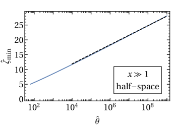
Figure 10: Rescaled position $\hat{\zeta}_{\text{min}}=\sqrt{x}\zeta_{\text{min}}$ of the minimum of the profile $\mathpzc{m}(\hat{\theta},\hat{\zeta})$ in the half-space $\zeta>0$ for $x\gg 1$ [Eq. 105] as a function of the rescaled time $\hat{\theta}=x^{2}\theta$. For $\hat{\zeta}_{\text{min}}\gg 1$ it turns out that the numerical data for $\hat{\zeta}_{\text{min}}$ are captured accurately by a logarithmic dependence on $\theta$: $\hat{\zeta}_{\text{min}}\simeq 1.4\times\ln(\hat{\theta})-1$ (dashed line). The numerical prefactor and the constant involved follow from a fit.

References

- Hohenberg and Halperin (1977) P. C. Hohenberg and B. I. Halperin, “Theory of dynamic critical phenomena,” Rev. Mod. Phys. 49, 435 (1977).
- Folk and Moser (2006) R. Folk and G. Moser, “Critical dynamics: a field-theoretical approach,” J. Phys. A 39, R207 (2006).
- Täuber (2014) U. C. Täuber, Critical Dynamics: A Field Theory Approach to Equilibrium and Non-Equilibrium Scaling Behavior (Cambridge University Press, 2014).
- Dietrich and Diehl (1983) S. Dietrich and H. W. Diehl, “The effects of surfaces on dynamic critical behavior,” Z. Phys. B 51, 343 (1983).
- Diehl and Janssen (1992) H. W. Diehl and H. K. Janssen, “Boundary conditions for the field theory of dynamic critical behavior in semi-infinite systems with conserved order parameter,” Phys. Rev. A 45, 7145 (1992).
- Diehl (1994) H. W. Diehl, “Universality classes for the dynamic surface critical behavior of systems with relaxational dynamics,” Phys. Rev. B 49, 2846 (1994).
- Wichmann and Diehl (1995) F. Wichmann and H. W. Diehl, “Dynamic surface critical behavior of systems with conserved bulk order parameter: Detailed RG analysis of the semi-infinite extensions of model B with and without nonconservative surface terms,” Z. Phys. B 97, 251 (1995).
- Ritschel and Czerner (1995) U. Ritschel and P. Czerner, “Universal Short-Time Behavior in Critical Dynamics near Surfaces,” Phys. Rev. Lett. 75, 3882 (1995).
- Majumdar and Sengupta (1996) S. N. Majumdar and A. M. Sengupta, “Nonequilibrium Dynamics following a Quench to the Critical Point in a Semi-infinite System,” Phys. Rev. Lett. 76, 2394 (1996).
- Pleimling (2004) M. Pleimling, “Aging phenomena in critical semi-infinite systems,” Phys. Rev. B 70, 104401 (2004).
- Diehl and Ritschel (1993) H. W. Diehl and U. Ritschel, “Dynamical relaxation and universal short-time behavior of finite systems,” J. Stat. Phys. 73, 1 (1993).
- Ritschel and Diehl (1995) U. Ritschel and H. W. Diehl, “Long-time traces of the initial condition in relaxation phenomena near criticality,” Phys. Rev. E 51, 5392 (1995).
- Ritschel and Diehl (1996) U. Ritschel and H. W. Diehl, “Dynamical relaxation and universal short-time behavior in finite systems. The renormalization-group approach,” Nucl. Phys. B 464, 512 (1996).
- Gambassi and Dietrich (2006) A. Gambassi and S. Dietrich, “Critical Dynamics in Thin Films,” J. Stat. Phys. 123, 929 (2006).
- Diehl and Chamati (2009) H. W. Diehl and H. Chamati, “Dynamic critical behavior of model A in films: Zero-mode boundary conditions and expansion near four dimensions,” Phys. Rev. B 79, 104301 (2009).
- Gambassi (2008) A. Gambassi, “Relaxation phenomena at criticality,” Eur. Phys. J. B 64, 379 (2008).
- Ball and Essery (1990) R. C. Ball and R. L. H. Essery, “Spinodal decomposition and pattern formation near surfaces,” J. Phys.: Condens. Matter 2, 10303 (1990).
- Binder and Frisch (1991) K. Binder and H. L. Frisch, “Dynamics of surface enrichment: A theory based on the Kawasaki spin-exchange model in the presence of a wall,” Z. Phys. B 84, 403 (1991).
- Puri and Frisch (1993) S. Puri and H. L. Frisch, “Dynamics of surface enrichment. Phenomenology and numerical results above the bulk critical temperature,” J. Chem. Phys. 99, 5560 (1993).
- Lee et al. (1999) B. P. Lee, J. F. Douglas, and S. C. Glotzer, “Filler-induced composition waves in phase-separating polymer blends,” Phys. Rev. E 60, 5812 (1999).
- Onuki (2002) A. Onuki, Phase Transition Dynamics (Cambridge University Press, 2002).
- Fisher and de Gennes (1978) M. E. Fisher and P. G. de Gennes, “Wall Phenomena in a Critical Binary Mixture,” C. R. Acad. Sci. Paris B 287, 207 (1978).
- Krech and Dietrich (1992) M. Krech and S. Dietrich, “Free energy and specific heat of critical films and surfaces,” Phys. Rev. A 46, 1886 (1992).
- Krech (1994) M. Krech, The Casimir effect in critical systems (World Scientific, Singapore, 1994).
- Brankov et al. (2000) J. G. Brankov, D. M. Dantchev, and N. S. Tonchev, The Theory of Critical Phenomena in Finite-Size Systems (World Scientific, Singapore, 2000).
- Gambassi (2009) A. Gambassi, “The Casimir effect: From quantum to critical fluctuations,” J. Phys.: Conf. Ser. 161, 012037 (2009).
- Brito et al. (2007) R. Brito, U. Marini Bettolo Marconi, and R. Soto, “Generalized Casimir forces in nonequilibrium systems,” Phys. Rev. E 76, 011113 (2007).
- Rodriguez-Lopez et al. (2011) P. Rodriguez-Lopez, R. Brito, and R. Soto, “Dynamical approach to the Casimir effect,” Phys. Rev. E 83, 031102 (2011).
- Dean and Gopinathan (2010) D. S. Dean and A. Gopinathan, “Out-of-equilibrium behavior of Casimir-type fluctuation-induced forces for free classical fields,” Phys. Rev. E 81, 041126 (2010).
- Dean et al. (2012) D. S. Dean, V. Demery, V. A. Parsegian, and R. Podgornik, “Out-of-equilibrium relaxation of the thermal Casimir effect in a model polarizable material,” Phys. Rev. E 85, 031108 (2012).
- Dean and Podgornik (2014) D. S. Dean and R. Podgornik, “Relaxation of the thermal Casimir force between net neutral plates containing Brownian charges,” Phys. Rev. E 89, 032117 (2014).
- Hanke (2013) A. Hanke, “Non-Equilibrium Casimir Force between Vibrating Plates,” PLOS ONE 8, e53228 (2013).
- Rohwer et al. (2017) C. M. Rohwer, M. Kardar, and M. Krüger, “Transient Casimir Forces from Quenches in Thermal and Active Matter,” Phys. Rev. Lett. 118, 015702 (2017).
- Gross et al. (2016) M. Gross, O. Vasilyev, A. Gambassi, and S. Dietrich, “Critical adsorption and critical Casimir forces in the canonical ensemble,” Phys. Rev. E 94, 022103 (2016).
- Gross et al. (2017) M. Gross, A. Gambassi, and S. Dietrich, “Statistical field theory with constraints: Application to critical Casimir forces in the canonical ensemble,” Phys. Rev. E 96, 022135 (2017).
- Diehl (1986) H. W. Diehl, “Field-theoretical Approach to Critical Behavior at Surfaces,” in Phase Transitions and Critical Phenomena, Vol. 10, edited by C. Domb and J. L. Lebowitz (Academic, London, 1986) p. 76.
- Pelissetto and Vicari (2002) A. Pelissetto and E. Vicari, “Critical phenomena and renormalization-group theory,” Phys. Rep. 368, 549 (2002).
- Gambassi et al. (2009) A. Gambassi, A. Maciolek, C. Hertlein, U. Nellen, L. Helden, C. Bechinger, and S. Dietrich, “Critical Casimir effect in classical binary liquid mixtures,” Phys. Rev. E 80, 061143 (2009).
- Note (1) Note that in Laplace space Eq. 20a, being time-independent, reduces to . These boundary conditions also fix the prefactor of the solution in Eq. 26.
- Poularikas (2010) A. D. Poularikas, Transforms and Applications Handbook, Third Edition (CRC Press, Boca Raton, FL, 2010).
- Abate and Valkó (2004) J. Abate and P. P. Valkó, “Multi-precision Laplace transform inversion,” Int. J. Num. Meth. Eng. 60, 979 (2004).
- Gradshteyn and Ryzhik (2014) I. S. Gradshteyn and I. M. Ryzhik, Table of Integrals, Series, and Products (Academic, London, 2014).
- Gross (2018) M. Gross, “First-passage dynamics of linear stochastic interface models: weak-noise theory and influence of boundary conditions,” J. Stat. Mech. Theor. Exp. 2018, 033213 (2018). ; M. Gross, “First-passage dynamics of linear stochastic interface models: numerical simulations and entropic repulsion effect,” J. Stat. Mech. Theor. Exp. 2018, 033212 (2018).
- Note (2) Upon performing the asymptotic expansion of the expression for given below Eq. 45, one has to take into account that because we assume .
- Note (3) This is formally a consequence of the lemma of Riemann-Lebesgue Bender and Orszag (1999).
- Note (4) The calculation is facilitated by using known Laplace transforms of hypergeometric functions (see §3.38.1 in Ref. Prudnikov (1992)).
- Olver et al. (2010) F. W. J. Olver, D. W. Lozier, R. F. Boisvert, and C. W. Clark, NIST Handbook of Mathematical Functions, 1st ed. (Cambridge University Press, 2010).
- Note (5) The asymptotic behaviors of a function in real space and in Laplace space are inter-related by means of so-called Tauberian theorems (see §XIII.5 in Ref. Feller (1971)).
- Note (6) The limit is singular because the initial condition [Eq. 16] is incompatible with the boundary conditions [Eq. 20a].
- Moin (2010) P. Moin, Fundamentals of Engineering Numerical Analysis, 2nd ed. (Cambridge University Press, 2010).
- Note (7) We have checked that by using as initial condition an equilibrium profile, which corresponds to a sufficiently high temperature , one obtains essentially the same results after a short transient period, which we do not consider here.
- Note (8) For large , the value of this prefactor becomes independent of .
- Note (9) In the case of model A dynamics, i.e., for , the dynamical stress tensor in Eq. 82 can be written as and thus reduces to the alternative formulation given in Eq. (56) in Ref. Dean and Gopinathan (2010) (apart from an overall minus sign in its definition).
- Krüger et al. (2018) M. Krüger, A. Solon, V. Demery, C. M. Rohwer, and D. S. Dean, “Stresses in non-equilibrium fluids: Exact formulation and coarse-grained theory,” J. Chem. Phys. 148, 084503 (2018).
- Note (10) The last expression in Eq. 94 follows by noting that, for an arbitrary function , one has .
- Roy et al. (2016) S. Roy, S. Dietrich, and F. Höfling, “Structure and dynamics of binary liquid mixtures near their continuous demixing transitions,” J. Chem. Phys. 145, 134505 (2016).
- Puosi et al. (2016) F. Puosi, D. L. Cardozo, S. Ciliberto, and P. C. W. Holdsworth, “Direct calculation of the critical Casimir force in a binary fluid,” Phys. Rev. E 94, 040102 (2016).
- Belardinelli et al. (2015) D. Belardinelli, M. Sbragaglia, L. Biferale, M. Gross, and F. Varnik, “Fluctuating multicomponent lattice Boltzmann model,” Phys. Rev. E 91, 023313 (2015).
- Furukawa et al. (2013) A. Furukawa, A. Gambassi, S. Dietrich, and H. Tanaka, “Nonequilibrium Critical Casimir Effect in Binary Fluids,” Phys. Rev. Lett. 111, 055701 (2013).
- Bender and Orszag (1999) C. M. Bender and S. A. Orszag, Advanced Mathematical Methods for Scientists and Engineers I: Asymptotic Methods and Perturbation Theory (Springer Science & Business Media, New York, NY, 1999).
- Prudnikov (1992) A. P. Prudnikov, Integrals and series, Vol. 4: Direct Laplace transforms, (Gordon and Breach, New York, NY, 1992).
- Feller (1971) W. Feller, An Introduction to Probability Theory and Its Applications, 2nd ed., Vol. 2 (John Wiley & Sons, Inc., New York, NY, 1971).