Cooling+Heating Flows in Galaxy clusters:
Turbulent heating, spectral modelling, and cooling efficiency

Abstract

The discrepancy between expected and observed cooling rates of X-ray emitting gas has led to the cooling flow problem at the cores of clusters of galaxies. A variety of models have been proposed to model the observed X-ray spectra and resolve the cooling flow problem, which involves heating the cold gas through different mechanisms. As a result, realistic models of X-ray spectra of galaxy clusters need to involve both heating and cooling mechanisms. In this paper, we argue that the heating time-scale is set by the magnetohydrodynamic (MHD) turbulent viscous heating for the Intracluster plasma, parametrised by the Shakura-Sunyaev viscosity parameter, $\alpha$. Using a cooling+heating flow model, we show that a value of $\alpha\simeq 0.05$ (with 10% scatter) provides improved fits to the X-ray spectra of cooling flow, while at the same time, predicting reasonable cooling efficiency, $\epsilon_{cool}=0.33^{+0.63}_{-0.15}$. Our inferred values for $\alpha$ based on X-ray spectra are also in line with direct measurements of turbulent pressure in simulations and observations of galaxy clusters. This simple picture unifies astrophysical accretion, as a balance of MHD turbulent heating and cooling, across more than 16 orders of magnitudes in scale, from neutron stars to galaxy clusters.

1. Introduction

The Intracluster Medium (ICM) of galaxy clusters consists of a plasma that is almost entirely ionized. This hot plasma radiates mostly in X-ray band which leads to a significant cooling of the ICM. At constant pressure, the cooling time of a plasma is the gas enthalpy divided by the energy lost per unit volume per unit time:

$$t_{\rm cool}\equiv\frac{5nk_{\rm B}T}{2n_{e}n_{H}\Lambda(T,Z)},$$ (1)

where $\Lambda(T,Z)$ is the cooling function in terms of temperature $T$ and metallicity $Z$, $n$ is the particle number density, and $k_{\rm B}$ is the Boltzmann’s constant. In the cores of clusters, the cooling time dips below $5\times 10^{8}$ yr, i.e. the inferred radiative cooling time of the gas in the central part, where X-ray emission is sharply peaked, is much shorter than the age of the cluster, which suggests the existence of cooling flow. The standard cooling flow model can be derived by combining continuity, Navier-Stokes and energy conservation equation that, after simplification, leads to:

$$\frac{dL_{X}}{dT}=\dot{M}\left(\frac{5k_{\rm B}}{2\mu m_{p}}-\frac{1dp}{\rho dT}\right).$$ (2)

In the case of constant pressure, we get the standard isobaric cooling flow model:

$$\frac{dL_{X}}{dT_{K}}=\frac{5\dot{M}k_{\rm B}}{2\mu m_{p}}.$$ (3)

X-ray spectroscopy has demonstrated that this model is inadequate and additional heating or cooling mechanisms should be incorporated into the model. Moreover, X-ray spectroscopy shows that the temperature drop toward the center is limited to about a factor of three. The cooling seems to be frozen precisely in the region where we expect more rapid cooling. In general, it appears that there is no strong evidence for any significant amount of cold X-ray emitting gas (below 1/3 of the maximum temperature) in any cluster Peterson & Fabian (2006).

There exist different manifestations of the cooling-flow problem: According to Peterson et al. (2003), there is the soft X-ray cooling-flow problem and the mass sink cooling-flow problem. The soft X-ray cooling-flow problem refers to the discrepancy seen between the predicted and observed soft X-ray spectrum, e.g. the lack of expected emission lines from a gas cooling to low temperatures at the core of the cluster. The mass sink cooling-flow problem refers to the lack of colossal mass deposition in cooling clusters from the hypothesized cooling-flow plasma.

Many mechanisms have been proposed to prevent the gas from cooling to low temperatures at the centers of cooling flows, such as the electron thermal conduction (Zakamska & Narayan 2003) , Mechanical heating of infalling gas in dense core systems (Khosroshahi et al. 2004) and turbulent heating (Zhuravleva et al. 2014), though the lead suspect amongst them is mechanical heating by Active Galactic Nuclei (AGN). AGN outbursts produce winds and intense radiation that can heat the gas. Produced weak shocks delay cooling of gas by reducing gas density and increasing the total energy David (2001); McNamara et al. (2005); Forman et al. (2005) or by compensating lost entropy of the gas Fabian et al. (2005). Moreover, viscous damping of sound waves generated by repeated AGN outbursts may represent a significant source of heating Fabian et al. (2003). Direct evidence for these sound waves came from the spectra observed by the Hitomi X-ray satellite, which measured the plasma’s line-of-sight velocity dispersion of $164\pm 10$ km/s within the core of Perseus cluster. This supports the hypothesis that turbulent dissipation of kinetic energy can supply enough heat to offset gas from cooling (Hitomi Collaboration et al. 2016).

In this paper,we provide a simple yet accurate thermodynamic model for cooling+heating (or CpH) flows, which captures the balance between turbulent heating and cooling in cluster cores (e.g., Zhuravleva et al. 2014). We then show that the model can simultaneously explain the X-ray spectra and the observed turbulent energy of the cluster cores, using a single parameter $\alpha\simeq 0.1$, for the Shakura-Sunyaev viscosity parameter, while at the same time, predict reasonable cooling efficiency. As such, this picture also unifies astrophysical accretion across 16 orders of magnitude in scale, from kilometres (around neutron stars and stellar black holes) to kiloparsecs (in cores of galaxy clusters).

2. Data and spectral Extraction

For this study, we use a sample of galaxy clusters presented by Hogan et al. (2017). The sample consists of 5 galaxy clusters observed with Chandra X-ray Observatory over long exposure times. All five clusters have a central cooling time $\leq 1\times 10^{9}$ yrs (Cavagnolo et al. 2009) suitable for our intended analysis. The data are obtained from the Chandra imaging online repository and analyzed using CIAO version 4.7. Bad pixels are masked out using the bad pixel map provided by the pipeline. Background flares are removed, and point sources are identified with the CIAO task WAVDETECT and masked out in all subsequent analysis. Finally, the blank-sky backgrounds are extracted for each target, and the images are prepared in the energy range 0.5–7.0 keV. In addition, cavities and filaments within ICM were masked clear, since these regions are usually out of equilibrium.

Because the cooling instabilities usually occur at small ($\lesssim$10 kpc) radii, we desire finely binned spectra in the central cluster regions. Our example clusters have deep Chandra data; as a result, choosing of annuli for spectral extraction is limited by resolution rather than the number of counts.

For each example cluster, concentric circular annuli are centered at the cluster center. The width of the central annulus is 3 pixels, where each pixel is 0.492 arcsec across. The width of each annulus increases in turn by 1-pixel until the sixth annulus, beyond which the width of each annulus is 1.5 times the width of the previous one with a total number of 10 annuli per source. For each obsid we have spectra alongside response matrix files (RMFs) and auxiliary response files (ARFs). We keep spectra separate before fitting them, but at the time of running the xspec we load them simultaneously.

Since emission from outer parts of the ICM affects and contaminates inter parts of spectra, we use deprojected spectra to obtain more accurate data. In order to fit observed data we load the extracted spectra for each cluster with their matched response files into xspec version 12.9.1 (Arnaud 1996) and use fixed values of $N_{H}$ reported in (Main et al. 2015).

Cluster	$N_{H}$	z	Scale	Observation IDs	Exposure (ks)	$\dot{M}_{SFR}$	$\dot{M}_{cool}$
	($10^{22}cm^{-2})$		(kpc/”)		Cleaned	$M_{\odot}yr^{-1}$	$M_{\odot}yr^{-1}$
A2029	0.033	0.0773	1.464	891, 4977, 6101	103.31	$0.8^{0.1}_{0.09}$	269.2 $\pm$ 1.1
A2199	0.039	0.0302	0.605	10748, 10803, 10804, 10805	119.61	$1^{9}_{1}$	47.9 $\pm$ 1.1
A496	0.040	0.0329	0.656	931, 4976	62.75	$0.18^{0.01}_{0.01}$	56.2 $\pm$ 1.1
A85	0.039	0.0551	1.071	904, 15173, 15174, 16263, 16264	193.64	$0.1^{2.5}_{0.1}$	87.1 $\pm$ 1.0
Hydra A	0.043	0.0550	1.069	4969, 4970	163.79	$4^{7}_{2}$	109.6 $\pm$ 1.0

Table 1 Sample clusters from Chandra data (Hogan et al. 2017). Standard cosmology with H0= 70 $km~{}s^{-1}~{}Mpc^{-1}$ has been used and scales are angular. The observed star formation rate ,$\dot{M}_{SFR}$, and classical cooling rate, $\dot{M}_{cool}$, is obtained from McDonald et al. (2018) and the K-band magnitude are collected from Gavazzi & Boselli (1996) and Jarrett et al. (2003) .

3. Modified cooling+heating (CpH) flow model: cooling v.s. sound crossing

AGNs outburst and jets can pump energy into the ICM (McNamara & Nulsen 2007). This can be done by shock waves or sound wave deposition close to the AGN. We introduce a new timescale, $t_{\rm heat}$, which represents time scale of the energy injection into the system by viscous heating. To estimate the heating time, we note that waves (and weak shocks) produced by AGcluster ofNs can travel at most by speed of sound. As a result, sound crossing time is the shortest time scale in the ICM. We further assume that heating or viscous time should be a multiple of sound crossing time

$$t_{\rm heat}=\alpha^{-3/2}t_{\rm sound}=\frac{R}{\alpha^{3/2}c_{s}}=R\sqrt{3\mu m_{p}\over 5\alpha^{3}k_{\rm B}T},$$ (4)

where $R$ is the distance to the center of the cluster, and $\alpha<1$. The $\alpha$ parameter quantifies the ratio of turbulent/magnetic to thermal energy, and is very similar to the Shakura-Sunyaev viscosity parameter in accretion disks (Shakura & Sunyaev 1973), as in a turbulent medium equipartition implies:

$$\langle v^{2}\rangle\sim\langle v^{2}_{A}\rangle\sim\alpha c^{2}_{s},$$ (5)

where $v$ and $v_{A}$ are turbulent and Alfven speeds. The heating time is then given by the ratio of thermal energy $nk_{\rm B}T$ by turbulent heating rate $\rho\langle v^{2}\rangle\frac{\langle v^{2}\rangle^{1/2}}{R}$:

$$t_{\rm heat}\sim\frac{nk_{\rm B}T}{\rho\langle v^{2}\rangle^{3/2}/R}\sim\frac{Rc^{2}_{s}}{\langle v^{2}\rangle^{3/2}}\sim\frac{R}{\alpha^{3/2}c_{s}}=\alpha^{-3/2}t_{\rm sound}.$$ (6)

The viscosity parameter typically takes a value of $\alpha\sim 0.01-0.1$ in magnetohydrodynamic (MHD) simulations of weakly magnetized plasmas (e.g., Salvesen et al. 2016).

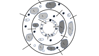
Now, the central idea of our proposal is that the main driver of thermal distribution in ICM is a balance of cooling and heating, governed by $t_{\rm cool}/t_{\rm sound}$ (in contrast to, e.g., thermal instability determined by $t_{\rm cool}/t_{\rm free-fall}$ McCourt et al. 2012; Hogan et al. 2017). Since $t_{\rm cool}$ drops faster than $T^{3/2}$ (at constant pressure; see below) while $t_{\rm heat}\propto t_{\rm sound}$ grows as $T^{-1/2}$ at low temperatures, the cold gas cools copiously, as in the standard cooling flows. However, the heating would win over the cooling for high temperatures. As a result, there is thermodynamic equilibrium at the temperature $T^{*}$ where $t_{\rm cool}(T^{*})\sim t_{\rm heat}(T^{*})$. In a (nearly) steady state (e.g., close to the cluster core), most of the gas would sit near this temperature . However, gas with $T\ll T^{*}$ would cool down to form atomic or molecular gas, and eventually stars. On the other hand gas with $T\gg T^{*}$ would heat up and eventually feed the cosmic ray population, through Fermi acceleration. This in-situ mass loss within each annulus should be replenished by a slow accretion/inflow of plasma from cluster outskirts, in steady state (see Figure 1 for a visual representation).

Figure 1.— Schematic illustration of cooling flow in each annulus. Here, we model temperature distribution within each annulus as a result of in-situ cooling and heating processes.

To see this more quantitatively, let’s begin with the cooling flow model. In the case of standard isobaric cooling flow model, we have:

$$\frac{5k_{\rm B}n}{2}\frac{dT}{dt}=-n_{e}n_{H}\Lambda(T,Z)$$ (7)

or

$$\frac{d\ln T}{dt}=-\frac{1}{t_{\rm cool}}.$$ (8)

To modify this, we add a heating term to the equation (8) and rewrite it as:

$$\frac{d\ln T}{dt}=-\frac{1}{t_{\rm cool}}+\frac{1}{t_{\rm heat}}$$ (9)

The mass-weighted probability distribution of $\ln T$ should satisfy the conservation equation:

$$\frac{\partial P(\ln T)}{\partial t}+\frac{\partial}{\partial\ln T}\left[P(\ln T)\frac{d\ln T}{dt}\right]=0,$$ (10)

which in steady state yields:

$$P(\ln T)\frac{d\ln T}{dt}=A={\rm const.}$$ (11)

Therefore the probability distribution takes the following form:

$$P_{CpH}(\ln T)=A\frac{t_{\rm cool}}{|1-\frac{t_{\rm cool}}{t_{\rm heat}}|},$$ (12)

where $A$ is a normalization constant that is fixed by requiring total integrated probability is 1:

$$A^{-1}=\int d\ln T\frac{t_{\rm cool}}{|1-\frac{t_{\rm cool}}{t_{\rm heat}}|}.$$ (13)

Now, as discussed above, we see from Equation (12) that when $t_{\rm cool}\ll t_{\rm heat}$ (or $T\ll T^{*}$), we obtain the standard cooling flow model. In contrast, if $t_{\rm cool}\gg t_{\rm heat}$ (or $T\gg T^{*}$) we have $P(\ln T)\approx t_{\rm heat}$.

Figure 2.— The emission measure for seventh annulus of A2029 with using mkcflow model and our CpH model.

4. A New Spectral Model

In the standard cooling flow model, the spectrum in steady state can be calculated using:

$$dL_{\rm cool}=n_{e}n_{H}\Lambda(T,Z)dV=\frac{5\dot{M}k_{\rm B}}{2\mu m_{p}}dT,$$ (14)

where $\dot{M}$ is the mass deposition rate, and $\mu$ is the mean molecular weight. We can re-express this equation in terms of a differential emission measure $dEM=n_{e}n_{H}dV$ which captures the differential distribution of plasma across temperatures:

$$\frac{dEM}{dT}=\frac{5\dot{M}k_{\rm B}}{2\mu m_{p}\Lambda(T,Z)}.$$ (15)

We can now convolve this distribution with the energy dependent line power $\frac{d\kappa}{dE}(E,T,Z)$ to produce an X-ray spectrum, which can be compared with observations. The spectral source model as a function of emission measure will be:

$$\frac{d\epsilon}{dE}=\int_{0}^{T_{\rm max}}\frac{dEM}{dT}\frac{d\kappa}{dE}(E,T,Z)dT,$$ (16)

where

$$\Lambda(T,Z)=\int_{0}^{\infty}dE\frac{d\kappa}{dE}(E,T,Z)E.$$ (17)

Equation (16), which is the prediction of the standard cooling flow model, cannot provide a good fit to the X-ray spectra of galaxy cluster cores (or outskirts) Peterson & Fabian (2006). In practice, it is common to use a single (or multi-) temperature model (so-called “mekal” in xspec) to fit the X-ray spectra, even though this cannot be physically justified given the short cooling times in cluster cores.

Our proposal to solve the problem is to apply the probability distribution 12 introduced in the previous section, which captures both heating and cooling in the flow. By plugging in the explicit expressions for of $t_{\rm cool}$ (Eq. 1), $t_{\rm heat}$ (Eq. 6) and pressure $p=nkT$ we find:

$$P_{CpH}(\ln T)=A\frac{t_{\rm cool}}{|1-\frac{f(T)}{f(T^{*})}|},$$ (18)

where

$$f(T)\equiv\frac{T^{5/2}}{\Lambda(T,Z)},~{}{\rm and}~{}~{}~{}f(T^{*})=\frac{n_{e}n_{H}}{n^{2}}\sqrt{12\mu m_{p}p^{2}R^{2}\over 125\alpha^{3}k_{\rm B}^{5}}$$ (19)

We can now modify the cooling flow emission measure $\frac{dEM}{dT}\rightarrow\frac{1}{|1-\frac{f(T)}{f(T^{*})}|}\frac{dEM}{dT}$ and apply it in the spectral model (16):

$$\frac{d\epsilon}{dE}=\int_{0}^{T_{max}}\frac{1}{|1-\frac{f(T)}{f(T^{*})}|}\frac{dEM}{dT}\frac{d\kappa}{dE}(E,T,Z)dT.$$ (20)

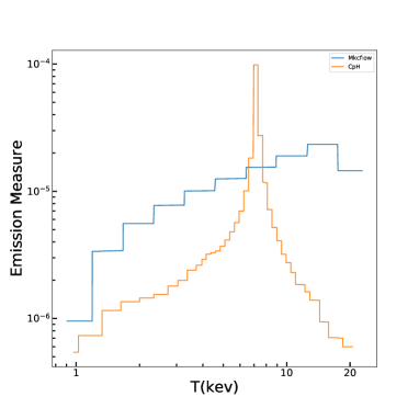
We fit the observed spectra after implementing our CpH model into the xspec. To do this, we modify the emission measure of the standard cooling flow (or “mkcflow”) model. To follow the changes in the emission measure after we implement our model into the xspec, we present an example of our best-fit emission measure of the cooling flow model, compared to our model, for the same cluster and the same annulus in Figure 2. In contrast to the mkcflow mode, which has a smooth emission measure, our model has a clear peak in temperature (where $T=T^{*}$ or $t_{\rm heat}=t_{\rm cool}$), as well as extended tails.

In order to fit observed Chandra spectra, $T^{*}$ is treated as a free parameter in xspec, while we fixed the lower and the upper limits of the integration $T_{\rm min}=10^{-2}$ keV and $T_{\rm max}=50$ keV. As such, our spectral model has the same number of parameters as a single-temperature (or mekal) model. It is worth mentioning that if the lower limit value of mkcflow model is set to such a small value, it is impossible to fit the observed data. In contrast, as we see below, we can find a good fit to data using the modified emission measure (20).

To obtain $\alpha$ we first compute the pressure , $p$ within each annulus of volume $V=4/3\pi(r^{3}_{out}-r^{3}_{in})$, as follows:

$$P(\ln T)=\frac{dM}{M_{tot}d\ln T}$$ (21)

$$\frac{dM}{d\ln T}=\mu m_{p}n\frac{dV}{d\ln T}=\mu m_{p}\frac{p}{k_{B}T}\frac{dV}{d\ln T}$$ (22)

By eliminating $dM$ in Eq. (22) using Eq. (21)and integrating over volume we get the following relation for $M_{tot}$:

$${M}_{tot}=\frac{\mu m_{p}pV}{\int k_{B}TP(\ln T)d\ln T}$$ (23)

We notice that normalization of the Eq. (18), $A$, has the inverse time dimension and as a result we define our mass deposition rate in each annulus as $\dot{M}_{cool}=AM_{tot}$. As a result after some simplification we can express pressure in terms of $\dot{M}_{cool}$ and $T^{*}$:

$$p^{2}=\frac{5\dot{M}}{2\mu m_{p}V}\int_{0}^{T_{max}}\frac{k_{B}^{3}T^{3}d\ln T}{\Lambda(T,Z)|1-\frac{f(T)}{f(T^{*})}|}$$ (24)

We can further express $n_{e}$ and $n_{H}$ in terms of the total number density $n$, using $n=n_{e}+n_{H}+n_{He}$, $X=n_{H}/(n_{H}+4n_{He})$ and $n_{e}=n_{H}+2n_{He}$, which yield

$$n_{e}=\frac{2X+2}{5X+3}n,\hskip 42.67912ptn_{H}=\frac{4X}{5X+3}n,$$ (25)

where $X$ is the hydrogen mass fraction and we shall consider $X\approx 0.75$. Now, by eliminating pressure $p$ in the following equation for $\alpha$ (26) and $f(T^{*})$ (Eq. 19), using Eq. (25) for $n_{e}$ and $n_{H}$, we find $\alpha$ which gives the value of viscosity parameter, within the annulus at radius $R$ and volume $V$, in terms of the X-ray observables $T^{*}$ and $\dot{M}$.

$$\alpha=\Big{[}\frac{125k^{5}_{\rm B}n^{4}f(T^{*})^{2}}{12n_{e}^{2}n_{H}^{2}\mu m_{p}p^{2}R^{2}}\Big{]}^{-1/3}$$ (26)

We name our model Cooling plus Heating (CpH) and it is publicly available at: https://heasarc.gsfc.nasa.gov/xanadu/xspec/manual/node158.html

5. Results

In this section, we probe our CpH model using the Chandra clusters sample and demonstrate that they are superior (or comparable) fits in cluster cores, in comparison to single-temperature mekal models. We then briefly discuss the implications for the cooling efficiency and turbulent viscosity in ICM.

We use xspec to fit Chandra X-ray data. For the single temperature model (phabs$\times$mekal) and our CpH model (phabs$\times$ CpH). We fix abundance to the solar and also fix the hydrogen column densities $N_{H}$ and redshifts to the values provided in Table (1). We ran Markov Chain Monte Carlo (MCMC) to find best-fit parameters. The best-fit parameter for single temperature model is $T$ and for our CpH model is $T^{*}$ (indicating the peak of the CpH probability distribution). The goodness of the fit and the best-fit parameters of our model, as well as the single temperature model, are provided in Table 2. We notice that the peaks of the temperature distribution in our best-fit models, $T^{*}$, happen to be close to the best-fit $T$ in the single-temperature models. However, typically our model provides a better (or comparable) fit to data in cluster cores (with an acceptable $\chi^{2}$ for the number of data points). In the cluster outskirts, where the assumption of a steady state cooling/heating flow is not valid, none of the models provide a good fit to the data. While the CpH and the mekal models provide satisfactory fits to X-ray data for the same annuli, the CpH model is preferred at $\Delta\chi^{2}=-56.9$ (or $7.5\sigma$ level) if we combine all the annuli with satisfactory fits.

Figure 3.— (a) (top) The measured MHD/turbulent viscous heating parameter $\alpha$, defined as the square of the ratio of sounds crossing to viscous dissipation time $\alpha=(t_{\rm heat}/t_{\rm sound})^{2/3}$. These values are inferred by fitting our CpH model to the spectra and fluxes of deprojected X-ray data from Chandra clusters. (b) (bottom) The 68% and 95% confidence regions for the mean $\bar{\alpha}$ and gaussian intrinsic scatter $\sigma$, assuming $\alpha=\bar{\alpha}\pm\sigma$.

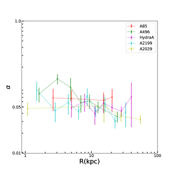
We can now plug our best-fit CpH spectral model into Eq. (26) to find the MHD/turbulent viscosity parameter $\alpha$, which is plotted in Figure 3. We find that a value of $\alpha\simeq 0.05$ (with a small intrinsic scatter of $\pm 10\%$) in the cluster cores (¡ 20-30 kpc, where CpH model can give a satisfactory fit to spectrum in Table 2). More precisely, measured $\alpha$’s are consistent with a gaussian distribution with mean $\bar{\alpha}$ and scatter $\sigma$ (see Figure 3b)

$$\bar{\alpha}=0.048^{+0.005}_{-0.006},~{}~{}\sigma=0.011^{+0.004}_{-0.006},$$ (27)

where errors reflect 1$\sigma$ uncertainties.

These values are consistent with viscosity parameters in shearing box accretion disk simulations Salvesen et al. (2016), as well as simulated (e.g., Gaspari & Churazov 2013) or observed turbulent energy fraction in cluster cores (Zhuravleva et al. 2014, 2016; Hitomi Collaboration et al. 2016).

Figure 4.— The predicted cold to hot gas density fraction accumulated over 7.7 Gyr (i.e. since $z=1$) , assuming our best-fit model and steady state.

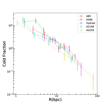
Considering that our proposed model is successful in representing the observed X-ray spectra, we can compare the mass deposition rate of our CpH model with the observed star formation rate. The key parameter for mass deposition rate is $\dot{M}$, which is directly provided by the spectral fitting in the XSPEC. Another useful quantity to be calculated is the ratio of cold to hot gas density, or cold fraction, which is $7.7~{}{\rm Gyr}\times A$. We estimate the cold fraction over a period of $\sim$ 7.7 Gyr (i.e. since $z=1$) for each cluster. The cold fraction is shown in Figure 4, which indicates that most of the cold gas is accumulated within the inner 10 kpc of cluster cores, where its density dominates the hot gas by up to an order of magnitude (we have used only “good fits” from Table 2, in Figs 3 and 4).

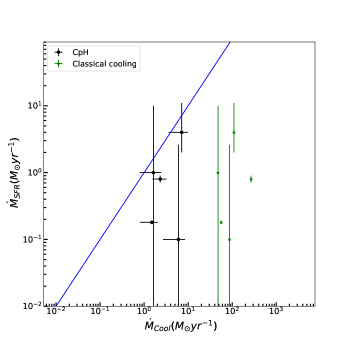
Let us assume that the cooled gas is used as fuel for star formation. We can define cooling efficiency as $\epsilon_{cool}\equiv\frac{\dot{M}_{SFR}}{\dot{M}_{cool}}$ from which we can specify how well AGN feedback can offset the runaway cooling. We have plotted $\dot{M}_{SFR}$ against $\dot{M}_{cool}$ for each cluster in Figure 5, showing that $\langle\dot{M}_{cool}\rangle_{\rm CpH}=3.7^{+0.8}_{-1.0}M_{\odot}/{\rm yr}$, while $\langle\dot{M}_{cool}\rangle_{\rm classical}\equiv M_{gas}(r<r_{cool})/t_{cool}=114\pm 0.5M_{\odot}/{\rm yr}$. Here in calculating $\dot{M}_{cool}$ for each cluster in the context of CpH model, we have considered and added the mass deposition rate of annuli that satisfy $A^{-1}<3Gyr$. This condition ensures that the thermodynamic equilibrium in an annulus at temperature $T^{*}$ has been established. On the other hand, in calculating the classical mass deposition rate $\dot{M}_{cool}$, the cooling radius $r_{cool}$ is defined as the radius within which cooling time $t_{cool}<3$ Gyr (McDonald et al. 2018). The observed star formation rates and classical cooling rates are reported in Table 1 in which the mean value of $\dot{M}_{SFR}$ is $1.2^{+2.3}_{-0.5}$. As a result we can calculate the cooling efficiency for underlying clusters which leads to $\epsilon_{cool}=0.33^{+0.63}_{-0.15}$ for CpH and $\epsilon_{cool}=0.01^{+0.02}_{-0.004}$ using results of McDonald et al. (2018). Based on these results we infer a much larger efficiency for star formation from cooling in the CpH model, i.e. $\epsilon_{cool}^{CpH}/\epsilon_{cool}^{classical}\sim 0.33/0.01\sim 33$ .

It worth mentioning that a clear advantage of our model compared to mkcflow model is that we have included the contribution of hot gas in all available temperatures and we have not omitted low temperature plasma while fitting the spectrum. In other words, even using all the hot gas to fit the spectrum, we have a consistent predicted viscosity parameter with observation and simulations, which can only be achieved for mkcflow model by introducing an unphysical low temperature cut-off.

Figure 5.— The observed star formation rates (McDonald et al. 2018) against mass deposition rates. Black points are results of using CpH and green stars are mass deposition rate within the cooling radius of $t_{cool}\leq 3Gyr$ (McDonald et al. 2018) for each cluster. The blue line represents $\dot{M}_{SFR}=\dot{M}_{cool}$.

6. conclusion

We have shown that by introducing a heating time-scale, modulated by sound-crossing time across the cluster, we can provide superior fits to the X-ray spectra of cores of galaxy clusters using a modified cooling(+heating) flow model, with the same number of parameters as the single-temperature model (CpH model is preferred to the mekal model at 7.5$\sigma$ level). As a byproduct, we find an MHD/turbulent viscosity parameter of $\alpha=0.048\pm 0.01$ (intrinsic scatter) $\pm 0.006$ ($1\sigma$ error), which is consistent with simulations and direct observations of turbulent energy fraction in cluster cores. The model can predict the cooling efficiency and the cold fraction by assuming a steady state for $\sim$ 7.7 Gyr (since $z\simeq 1$), providing a concrete solution to the cooling flow problem. The cooling efficiency of CpH is $\epsilon_{cool}=0.33^{+0.63}_{-0.15}$ which is much more larger than classic cooling efficiency $\epsilon_{cool}=0.01^{+0.02}_{-0.004}$ within cooling radius of $r(t_{cool}<3Gyr)$. Furthermore, this model unifies the picture of astrophysical accretion, as a balance of MHD turbulent heating and cooling, across 16 orders of magnitude in scale (from neutron stars and X-ray binaries to cluster cores).

Cluster	$R(kpc)$	$\chi^{2}_{CpH}$	$\chi^{2}_{{\it mekal}}$	$T^{*}(keV)$	$T_{{\it mekal}}(keV)$	$\dot{M}(M_{\odot}/yr)$	$L_{x}(erg/s)$	$Net\_counts$	$N_{d.o.f}$
	1.49$\pm 0.6$	62	66	$1.4^{+0.4}_{-0.5}$	1.3 ${}^{+0.3}_{-0.4}$	$0.1^{+0.04}_{-0.05}$	$6.76^{+0.86}_{-0.88}\times 10^{40}$	3300
	2.83$\pm 0.74$	66	66	$3.0^{+1.1}_{-0.7}$	2.5${}^{+0.7}_{-0.4}$	$0.12^{+0.06}_{-0.07}$	$2.89^{+0.19}_{-0.22}\times 10^{41}$	7203
	4.46$\pm 0.89$	60	61	$2.8^{+0.7}_{-0.5}$	2.4${}^{+0.5}_{-0.3}$	$0.26^{+0.09}_{-0.12}$	$5.35^{+0.34}_{-0.27}\times 10^{41}$	11695
	6.40$\pm 1.04$	61	61	$2.5^{+0.4}_{-0.3}$	2.3${}^{+0.4}_{-0.2}$	$0.14^{+0.16}_{-0.11}$	$7.7^{+0.36}_{-0.38}\times 10^{41}$	16671
A2199	8.63 $\pm 1.19$	76	82	$2.9^{+0.3}_{-0.5}$	2.5${}^{+0.2}_{-0.2}$	$0.75^{+0.19}_{-0.28}$	$16.5^{+0.4}_{-0.5}\times 10^{41}$	21142	64
	11.61 $\pm 1.79$	62	62	$2.9^{+0.3}_{-0.3}$	2.7${}^{+0.2}_{-0.2}$	$0.27^{+0.28}_{-0.20}$	$21.0^{+0.4}_{-0.5}\times 10^{41}$	28883
	16.07$\pm 2.68$	63	66	$2.8^{+0.5}_{-0.6}$	2.5${}^{+0.3}_{-0.3}$	$0.73^{+0.33}_{-0.41}$	$18.7^{+0.65}_{-0.52}\times 10^{41}$	38885
	22.77$\pm 4.01$	57	56	$3.3^{+0.6}_{-0.4}$	3.1${}^{+0.3}_{-0.3}$	$0.33^{+0.33}_{-0.25}$	$32.5^{+0.74}_{-0.67}\times 10^{41}$	68880
	32.97 $\pm 6.18$	47	48	$4.4^{+0.5}_{-0.5}$	3.9${}^{+0.3}_{-0.3}$	$1.1^{+0.7}_{-0.7}$	$76.5^{+0.89}_{-0.93}\times 10^{41}$	127922
	48.2$\pm 9.08$	101	105	$4.7^{+0.2}_{-0.3}$	4.4${}^{+0.1}_{-0.1}$	$2.2^{+1.1}_{-1.1}$	$243^{+1.4}_{-1.3}\times 10^{41}$	216253
	5.00$\pm 1.3$	19	28	$3.7^{+0.9}_{-0.7}$	$3.1^{+0.5}_{-0.4}$	$1.6^{+0.3}_{-0.4}$	$9.5^{+0.35}_{-0.33}\times 10^{41}$	7241
	7.89$\pm 1.6$	17	20	$4^{+1.0}_{-0.7}$	$3.3^{+0.5}_{-0.4}$	$1.5^{+0.4}_{-0.6}$	$16.2^{+0.64}_{-0.5}\times 10^{41}$	9862
	11.31 $\pm 1.8$	21	22	$3.0^{+0.7}_{-0.6}$	$2.5^{+0.4}_{-0.4}$	$1.5^{+0.6}_{-0.9}$	$16.0^{+0.5}_{-0.6}\times 10^{41}$	16102
	15.25$\pm 2.1$	27	27	$5^{+2.0}_{-1.4}$	$3.7^{+1.0}_{-0.8}$	$1.1^{+0.4}_{-0.6}$	$20.6^{+0.9}_{-1.9}\times 10^{41}$	20226
HydraA	20.51$\pm 3.2$	14	14	$3.2^{+0.7}_{-0.5}$	$2.8^{+0.4}_{-0.3}$	$2.5^{+1.4}_{-1.7}$	$32.1^{+1.0}_{-1.0}\times 10^{41}$	26833	21
	28.40 $\pm 4.7$	22	23	$3.5^{+0.8}_{-0.3}$	$3.1^{+0.3}_{-0.2}$	$3.7^{+2.6}_{-2.6}$	$73.1^{+1.2}_{-1.1}\times 10^{41}$	44738
	40.24$\pm 7.1$	25	33	$4.4^{+0.6}_{-0.5}$	$3.7^{+0.3}_{-0.2}$	$7.7^{+3.3}_{-3.6}$	$124^{+1.6}_{-1.7}\times 10^{41}$	68412
	58.25 $\pm 10.9$	36	42	$4.5^{+0.4}_{-0.1}$	$4.2^{+0.1}_{-0.1}$	$8.2^{+6.1}_{-3.9}$	$258^{+1.9}_{-2.1}\times 10^{41}$	111067
	85.20$\pm 16.0$	67	87	$4.6^{+0.3}_{-0.2}$	$4.3^{+0.1}_{-0.1}$	$13.4^{+6.7}_{-5.6}$	$409^{+2.7}_{-2.0}\times 10^{41}$	145225
	125.2$\pm 23.9$	45	64	$4.6^{+0.3}_{-0.2}$	$4.2^{+0.1}_{-0.1}$	$14.4^{+7.2}_{-7.2}$	$388^{+2.0}_{-1.9}\times 10^{41}$	153239
	1.08$\pm 1.0$	63	63	$2.6^{+0.3}_{-0.65}$	2.2${}^{+0.4}_{-0.3}$	$0.21^{+0.24}_{-0.17}$	$4.2^{+0.1}_{-0.18}\times 10^{41}$	1993
	3.60$\pm 1.44$	103	103	$3.0^{+0.6}_{-0.4}$	2.8${}^{+0.4}_{-0.3}$	$0.31^{+0.40}_{-0.24}$	$35.2^{+2.0}_{-3.6}\times 10^{41}$	12208
	6.84$\pm 1.8$	104	104	$3.1^{+0.5}_{-0.2}$	2.9${}^{+0.5}_{-0.3}$	$0.50^{+0.67}_{-0.40}$	$49.7^{+1.1}_{-1.7}\times 10^{41}$	13500
	10.80$\pm 2.16$	105	106	$11.7^{+2.7}_{-3.4}$	7.8${}^{+3.2}_{-1.8}$	$1.3^{+0.4}_{-0.6}$	$91.4^{+2.8}_{-3.0}\times 10^{41}$	22702
A2029	15.49 $\pm 2.5$	98	97	$5.6^{+2.2}_{-1.2}$	4.5${}^{+0.9}_{-0.6}$	$1.8^{+1.6}_{-1.4}$	$12.9^{+0.4}_{-0.3}\times 10^{42}$	28949	86
	20.89$\pm 2.88$	110	110	$9.6^{+4.1}_{-3.0}$	6.4 ${}^{+1.2}_{-1.0}$	$2.3^{+1.3}_{-1.6}$	$19.1^{+0.3}_{-0.6}\times 10^{42}$	34104
	28.09$\pm 4.32$	77	77	$7.2^{+2.4}_{-1.3}$	6.0${}^{+0.8}_{-0.5}$	$2.9^{+3.0}_{-2.2}$	$33.3^{+0.5}_{-0.5}\times 10^{42}$	56203
	38.90 $\pm 6.48$	117	117	$8.1^{+1.7}_{-0.8}$	6.9${}^{+0.5}_{-0.5}$	$4.0^{+3.7}_{-2.9}$	$63.8^{+0.6}_{-0.5}\times 10^{42}$	88105
	55.10$\pm 9.72$	101	101	$7.2^{+1.8}_{-1.9}$	7.4 ${}^{+0.5}_{-0.4}$	$1.7^{+1.7}_{-1.3}$	$99.8^{+0.8}_{-0.3}\times 10^{42}$	128336
	79.77$\pm 14.95$	104	102	$8.9^{+1.0}_{-0.8}$	7.8${}^{+0.4}_{-0.3}$	$3.6^{+6.4}_{-3.5}$	$165^{+1.0}_{-1.0}\times 10^{42}$	171978
	1.61$\pm 0.65$	5	9	$1.7^{+0.6}_{-0.4}$	1.4${}^{+0.44}_{-0.19}$	$0.15^{+0.06}_{-0.06}$	$1.3^{+0.1}_{-0.1}\times 10^{41}$	533
	3.07 $\pm 0.81$	4	10	$1.3^{+0.2}_{-0.2}$	1.1${}^{+0.2}_{-0.1}$	$0.47^{+0.10}_{-0.15}$	$2.7^{+0.2}_{-0.2}\times 10^{41}$	2156
	4.84$\pm 0.97$	6	8	$1.8^{+0.5}_{-0.2}$	1.7${}^{+0.2}_{-0.2}$	$0.50^{+0.17}_{-0.22}$	$5.6^{+0.4}_{-0.4}\times 10^{40}$	4680
	6.94$\pm 1.13$	7	7	$2.9^{+1.2}_{-0.8}$	2.3${}^{+0.6}_{-0.3}$	$0.38^{+0.20}_{-0.25}$	$10.1^{+0.6}_{-0.5}\times 10^{41}$	7361
A496	9.36$\pm 1.29$	6	6	$2.8^{+0.8}_{-0.6}$	2.3${}^{+0.5}_{-0.2}$	$0.51^{+0.37}_{-0.33}$	$15.9^{+0.5}_{-0.6}\times 10^{41}$	10129	10
	12.59$\pm 1.94$	12	11	$2.4^{+0.8}_{-0.2}$	2.2${}^{+0.2}_{-0.1}$	$0.52^{+0.37}_{-0.39}$	$32.6^{+0.8}_{-0.7}\times 10^{41}$	13736
	17.43$\pm 2.90$	24	24	$2.9^{+0.3}_{-0.3}$	2.7 ${}^{+0.1}_{-0.1}$	$0.37^{+0.26}_{-0.29}$	$48.6^{+1.0}_{-0.8}\times 10^{41}$	21962
	24.69$\pm 4.36$	7	6	$3.2^{+0.4}_{-0.3}$	3.0${}^{+0.3}_{-0.2}$	$0.55^{+0.55}_{-0.44}$	$80.4^{+1.2}_{-1.1}\times 10^{41}$	31017
	35.74$\pm 6.70$	24	23	$4.1^{+0.3}_{-0.5}$	3.8${}^{+0.2}_{-0.2}$	$0.71^{+0.71}_{-0.57}$	$122^{+1.2}_{-1.3}\times 10^{41}$	46112
	52.29$\pm 9.84$	19	19	$4.3^{+0.6}_{-0.3}$	4.0${}^{+0.2}_{-0.2}$	$1.1^{+1.1}_{-1.0}$	$194^{+1.7}_{-1.1}\times 10^{41}$	64190
	2.63 $\pm 1.1$	23	22	$2.4^{+1.1}_{-0.6}$	1.98${}^{+0.7}_{-0.3}$	$0.34^{+0.18}_{-0.17}$	$5.2^{+0.4}_{-0.4}\times 10^{41}$	3503
	5.0$\pm 1.32$	23	22	$3^{+1.1}_{-0.7}$	2.4${}^{+0.7}_{-0.4}$	$0.68^{+0.29}_{-0.36}$	$14.7^{+0.8}_{-0.9}\times 10^{41}$	8458
	7.90$\pm 1.58$	38	39	$2.7^{+0.4}_{-0.4}$	2.2${}^{+0.4}_{-0.2}$	$1.69^{+0.51}_{-0.79}$	$32.3^{+1.2}_{-1.4}\times 10^{41}$	11147
	11.33$\pm 1.84$	98	98	$2.6^{+0.4}_{-0.3}$	2.3${}^{+0.1}_{-0.1}$	$1.96^{+0.90}_{-1.2}$	$42.5^{+1.3}_{-1.3}\times 10^{41}$	14413
A85	15.28$\pm 2.11$	32	32	$3.6^{+1.1}_{-0.8}$	2.8${}^{+0.6}_{-0.4}$	$1.4^{+0.6}_{-0.8}$	$39.4^{+1.2}_{-2.2}\times 10^{41}$	16205	24
	20.55$\pm 3.16$	22	28	$3.3^{+0.9}_{-0.6}$	2.8${}^{+0.6}_{-0.4}$	$2.3^{+0.6}_{-0.6}$	$52.0^{+2.2}_{-1.5}\times 10^{41}$	26093
	28.45$\pm 4.74$	93	93	$4.4^{+1}_{-0.8}$	3.8${}^{+0.3}_{-0.3}$	$3.7^{+0.7}_{-2.9}$	$143^{+2.0}_{-2.4}\times 10^{41}$	46348
	40.31$\pm 7.11$	73	73	$5.8^{+1.3}_{-1}$	4.6${}^{+0.2}_{-0.2}$	$3.3^{+2.2}_{-2.2}$	$223^{+3}_{-2}\times 10^{41}$	68838
	58.36 $\pm 10.93$	198	198	$6.4^{+1.2}_{-1}$	5.1${}^{+0.2}_{-0.2}$	$5.3^{+3.2}_{-4.9}$	$381^{+3.2}_{-2.2}\times 10^{41}$	105746
	85.36$\pm 16.10$	278	278	$6.7^{+1.3}_{-0.7}$	5.8${}^{+0.2}_{-0.2}$	$3.4^{+4.5}_{-2.2}$	$556^{+4.7}_{-3.5}\times 10^{41}$	134958

Table 2Calculated best-fit $\chi^{2}$ of our CpH model and mekal single-temperature model, with the best-fit parameters of fitting for the first ten annuli. $T^{*}$ and $\dot{M}$ are best fit parameters of our CpH model. The red (italic) fonts suggest that the fit is outside the 90% expected range for the (reduced) $\chi^{2}$ for $N_{d.o.f}$, i.e. it is not a good fit. We see that our CpH model typically provides a lower $\chi^{2}$, or a better fit, in cluster cores.

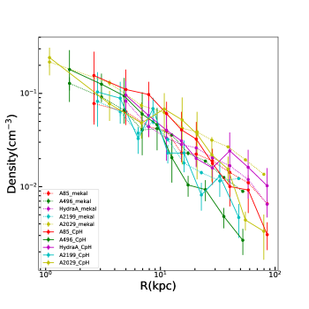
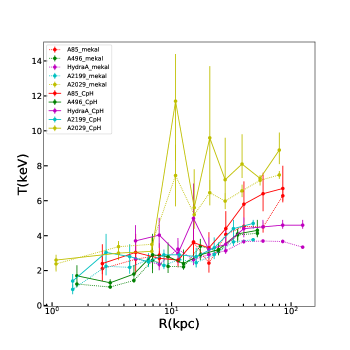
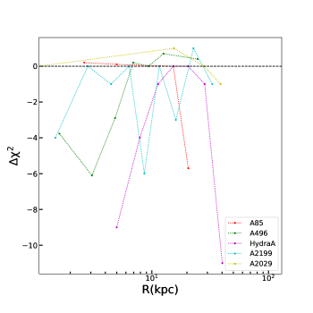
In the appendix we are providing temperature, density and $\Delta\chi^{2}$ profiles of CpH and Mekal model. Figure 6 shows the close proximity of the density profiles in CpH and Mekal Model (Data of Mekal profiles are extracted from Hogan et al. (2017)). As can be inferred from Figure 6 the peak temperature profiles of CpH and Mekal temperatures profiles show almost the same trend. In order to verify that the CpH model provides an improved fit over the Mekal model, we present the $\Delta\chi^{2}=\chi^{2}_{CpH}-\chi^{2}_{Mekal}$ profile in Figure 7 in which we are using only good fits (black bins in Table 2).

Figure 6.— Deprojected density and temperature profiles of CpH (solid lines) compared with what Hogan et al. (2017) found using Mekal (dotted lines).

Figure 7.— $\Delta\chi^{2}$ profile based on good fits in Table 2. It is apparent from this plot that the majority of bins have lower $\chi^{2}$ for CpH with respect to Mekal.

References

- Arnaud (1996) Arnaud, K. A. 1996, Astronomical Data Analysis Software and Systems V, 101, 17
- Balucinska-Church & McCammon (1992) Balucinska-Church, M., & McCammon, D. 1992, ApJ, 400, 699
- Cappellari et al. (2006) Cappellari, M., Bacon, R., Bureau, M., et al. 2006, MNRAS, 366, 1126
- Cavagnolo et al. (2009) Cavagnolo, K. W., Donahue, M., Voit, G. M., & Sun, M. 2009, ApJS, 182, 12
- David (2001) David, L. 2001, Chandra Proposal,
- Fabian et al. (2005) Fabian, A. C., Reynolds, C. S., Taylor, G. B., & Dunn, R. J. H. 2005, MNRAS, 363, 891
- Fabian et al. (2003) Fabian, A. C., Sanders, J. S., Allen, S. W., et al. 2003, MNRAS, 344, L43
- Fruscione et al. (2006) Fruscione, A., McDowell, J. C., Allen, G. E., et al. 2006, Proc. SPIE, 6270, 62701V
- Freeman et al. (2002) Freeman, P. E., Kashyap, V., Rosner, R., & Lamb, D. Q. 2002, ApJS, 138, 185
- Gaspari & Churazov (2013) Gaspari, M., & Churazov, E. 2013, A&A, 559, A78
- Gavazzi & Boselli (1996) Gavazzi, G., & Boselli, A. 1996, Astrophysical Letters and Communications, 35, 1
- Hitomi Collaboration et al. (2016) Hitomi Collaboration, Aharonian, F., Akamatsu, H., et al. 2016, Nature, 535, 117
- Hogan et al. (2017) Hogan, M. T., McNamara, B. R., Pulido, F., et al. 2017, ApJ, 837, 51
- Jarrett et al. (2003) Jarrett, T. H., Chester, T., Cutri, R., Schneider, S. E., & Huchra, J. P. 2003, AJ, 125, 525
- Kalberla et al. (2005) Kalberla, P. M. W., Burton, W. B., Hartmann, D., et al. 2005, A&A, 440, 775
- Khosroshahi et al. (2004) Khosroshahi, H. G., Jones, L. R., & Ponman, T. J. 2004, MNRAS, 349, 1240
- Landau & Lifshitz (1969) Landau, L. D., & Lifshitz, E. M. 1969, Course of Theoretical Physics, Oxford: Pergamon Press, 1969, 2nd ed.,
- Liedahl et al. (1995) Liedahl, D. A., Osterheld, A. L., & Goldstein, W. H. 1995, ApJ, 438, L115
- Main et al. (2015) Main, R., McNamara, B., Nulsen, P., Russell, H., & Vantyghem, A. 2015, arXiv:1510.07046
- McNamara et al. (2005) McNamara, B. R., Nulsen, P. E. J., Wise, M. W., et al. 2005, Nature, 433, 45
- McNamara & Nulsen (2007) McNamara, B. R., & Nulsen, P. E. J. 2007, ARA&A, 45, 117
- Forman et al. (2005) Forman, W., Nulsen, P., Heinz, S., et al. 2005, ApJ, 635, 894
- McCourt et al. (2012) McCourt, M., Sharma, P., Quataert, E., & Parrish, I. J. 2012, MNRAS, 419, 3319
- McDonald et al. (2018) McDonald, M., Gaspari, M., McNamara, B. R., et al. 2018, ApJ, 858, 45.
- Mewe et al. (1985) Mewe, R., Gronenschild, E. H. B. M., & van den Oord, G. H. J. 1985, A&AS, 62, 197
- Mewe et al. (1986) Mewe, R., Lemen, J. R., & van den Oord, G. H. J. 1986, A&AS, 65, 511
- Padmanabhan et al. (2004) Padmanabhan, N., Seljak, U., Strauss, M. A., et al. 2004, New A, 9, 329
- Peterson & Fabian (2006) Peterson, J. R., & Fabian, A. C. 2006, Phys. Rep., 427, 1
- Peterson et al. (2003) Peterson, J. R., Kahn, S. M., Paerels, F. B. S., et al. 2003, ApJ, 590, 207
- Russell et al. (2008) Russell, H. R., Sanders, J. S., & Fabian, A. C. 2008, MNRAS, 390, 1207
- Sanders & Fabian (2007) Sanders, J. S., & Fabian, A. C. 2007, MNRAS, 381, 1381
- Sanders & Fabian (2008) Sanders, J. S., & Fabian, A. C. 2008, MNRAS, 390, L93
- Shakura & Sunyaev (1973) Shakura, N. I., & Sunyaev, R. A. 1973, A&A, 24, 337
- Salvesen et al. (2016) Salvesen, G., Simon, J. B., Armitage, P. J., & Begelman, M. C. 2016, MNRAS, 457, 857
- Zhuravleva et al. (2014) Zhuravleva, I., Churazov, E., Schekochihin, A. A., et al. 2014, Nature, 515, 85
- Zhuravleva et al. (2016) Zhuravleva, I., Churazov, E., Arévalo, P., et al. 2016, MNRAS, 458, 2902
- Zakamska & Narayan (2003) Zakamska, N. L., & Narayan, R. 2003, ApJ, 582, 162