Hermite–Padé polynomials and analytic continuation: new approach and some results

Abstract

We discuss a new approach to realization of the well-known Weierstrass’s programme on efficient continuation of an analytic element corresponding to a multivalued analytic function with finite number of branch points. Our approach is based on the use of Hermite–Padé polynomials.

Bibliography: [51] titles.

Keywords: analytic continuation, Weierstrass approach, Hermite–Padé polynomials, distribution of zeros, Riemann surface.

1 Introduction and statement of the problem

1.1

The problem of analytic continuation of power series beyond its disc of convergence is a well-known problem in complex analysis, which also has important applications. In the present paper, we discuss this problem from the point of view of Weierstrass’s approach to the concept of analytic functions, which depends on the local representation of an analytic function as a power series with centre at some point of the Riemann sphere $\overline{\mathbb{C}}$. For more on this approach, see, prima facie, the book [10], and also [11], [34], [28, Ch. 8], [7], [8], [9].

The purpose of the present paper is to introduce and briefly discuss a new approach to the efficient solution of the analytic continuation problem for power series residing on the use of Hermite–Padé polynomials and some extensions thereof. In §§ 2 and 3 we formulate some new theoretical results in this direction which we have been able to derive so far. In § 5 we briefly discuss the most straightforward, to our opinion, applications of our theoretical results in the study of applied problems. In particular, in § 5 we illustrate our approach and theoretical results on some numerical examples pertaining to the model class of multivalued analytic functions considered in the present paper (see § 1.2 below).

We plan to prove the theoretical results of the present study in the separate papers [49] and [50]. We also intend to give a more detailed analysis of possible applications of the method proposed here in applied problems involving analytic continuation.

The new approach proposed below to efficient solution of the analytic continuation problem for power series beyond its disc of convergence will be demonstrated (from the theoretical as well as the numerical standpoints) on an example of some ‘‘model’’ class of multivalued analytic functions based on the use of the inverse of the Zhukovskii function (see representation (1) below). This class was first introduced in [45] (see also the papers [46], [48]), where it was denoted by $\mathscr{Z}$. Below, this notation will be retained, but when required the parameters in representation (1) will be refined.

1.2

Let $\Delta_{1}:=[-1,1]$, $\varphi(z):=z+(z^{2}-1)^{1/2}$, $z\notin\Delta_{1}$, be the inverse of the Zhukovskii function; here and in what follows we choose the branch of the root function such that $(z^{2}-1)^{1/2}/z\to 1$ as $z\to\infty$. The function $\varphi(z)$ is meromorphic in the domain $D_{1}:=\overline{\mathbb{C}}\setminus\Delta_{1}$ ($\varphi$ maps $D_{1}$ conformally and univalently onto the exterior $\overline{\mathbb{C}}\setminus\overline{\mathbb{D}}$ of the unit disc $\mathbb{D}:=\{z:|z|<1\}$). In the domain $\overline{\mathbb{C}}\setminus\{-1,1\}$ the function $\varphi$ is already a multivalued (more precisely, two-valued) analytic function.

Let $A_{j}\in\mathbb{C}$, $j=1,\dots,m$, be arbitrary pairwise distinct complex numbers such that $|A_{j}|>1$. Consider the function

$$f(z):=\prod_{j=1}^{m}\left(A_{j}-\frac{1}{\varphi(z)}\right)^{\alpha_{j}},\quad z\in D_{1},$$ (1)

where $\alpha_{j}\in\mathbb{C}\setminus\mathbb{Z}$, $\sum_{j=1}^{m}\alpha_{j}\in\mathbb{Z}$ (note that for the above branch of the root function we have $1/\varphi(z)=z-(z^{2}-1)^{1/2}$). Since $(A_{j}-1/\varphi(z))\neq 0$ for $z\in D_{1}$ under the above conditions on $A_{j}$ and with the above choice of the branch of the root function, we can find a holomorphic (i.e., singlevalued analytic) branch $f\in\mathscr{H}(D_{1})$ of the function $f$ in the domain $D_{1}$. In the domain $\overline{\mathbb{C}}\setminus\{-1,1\}$ the analytic function $f$ is not anymore singlevalued. In addition to the second-order branch points $z=\pm 1$, this function has branches at the points $a_{j}=(A_{j}+1/A_{j})/2\in\mathbb{C}\setminus\Delta_{1}$, $j=1,\dots,m$, of (in general) infinite order (if $\alpha_{j}\in\mathbb{C}\setminus\mathbb{Q}$ for the corresponding $A_{j}$). Thus, the total set of branch points of a function $f$ of the form (1) is $\Sigma=\Sigma(f)=\{\pm 1,a_{j},j=1,\dots,m\}$.

In what follows, for an arbitrary $n\in\mathbb{N}$, we denote by $\mathbb{P}_{n}:=\mathbb{C}[z]$ the space of all algebraic polynomials of degree $\leqslant{n}$, $\mathbb{P}^{*}_{n}:=\mathbb{P}_{n}\setminus\{0\}$. Given an arbitrary polynomial $Q\in\mathbb{C}[z]$, $Q\not\equiv 0$, we let

$$\chi(Q):=\sum_{\zeta:Q(\zeta)=0}\delta_{\zeta}$$

demote the measure counting the zeros (with multiplicities) of the polynomial $Q$.

The weak convergence in the space of measures will be denoted by ‘‘$\overset{*}{\longrightarrow}$’’.

For an arbitrary (positive Borel) measure $\mu$, $\operatorname{supp}{\mu}\subset\mathbb{C}$, we denote by $V^{\mu}$ the logarithmic potential of $\mu$,

$$V^{\mu}(z):=\int\log\frac{1}{|z-\zeta|}\,d\mu(\zeta).$$

By ‘‘$\overset{\operatorname{cap}}{\longrightarrow}$’’ we shall denote the convergence with respect to the (logarithmic) capacity on compact subsets of some domain.

Below, ‘‘$\sqrt{\,\cdot\,}\,$’’ means the principle square root of a nonnegative real number, $\sqrt{a^{2}}=|a|$, $a\in\mathbb{R}$.

Given a function $f\in\mathscr{H}(D_{1})$, we fix some germ

$$f_{\infty}=\sum_{k=0}^{\infty}\frac{c_{k}}{z^{k}},$$

holomorphic at the point $z=\infty$, $f_{\infty}\in\mathscr{H}(\infty)$.

For a fixed germ $f_{\infty}\in\mathscr{H}(\infty)$ and an arbitrary $n\in\mathbb{N}$, we denote by $P_{n}$ and $Q_{n}$, $P_{n},Q_{n}\in\mathbb{P}_{n}:=\mathbb{C}[z]$, $Q_{n}\not\equiv 0$, the polynomials defined (not uniquely) from the relation

$$(Q_{n}f_{\infty}-P_{n})(z)=O\left(\frac{1}{z^{n+1}}\right),\quad z\to\infty.$$ (2)

The rational function $[n/n]_{f_{\infty}}:=P_{n}/Q_{n}$, which is uniquely determined, is called the diagonal Padé approximant (the ‘‘diagonal PA’’ or simply ‘‘PA’’) of the germ $f_{\infty}$ at the point $z=\infty$.

The next facts (3)–(5) follow from Stahl’s theory (see [42], [43], and also [4] and [44]):

$$\frac{1}{n}\chi(P_{n}),\frac{1}{n}\chi(Q_{n})\overset{*}{\longrightarrow}\tau_{\Delta_{1}},\quad n\to\infty,$$ (3)

here $\tau^{\vphantom{p}}_{\Delta_{1}}=\dfrac{1}{\pi}\dfrac{dx}{\sqrt{1-x^{2}}}$ is the unit Robin measure of the interval $\Delta_{1}$; i.e., $V^{\tau^{\vphantom{p}}_{\Delta_{1}}}(x)\equiv\operatorname{const}=\gamma_{\Delta_{1}}$, and $\gamma_{\Delta_{1}}$ is the Robin constant for the interval $\Delta_{1}$;

$$[n/n]_{f_{\infty}}(z)\overset{\operatorname{cap}}{\longrightarrow}f(z)\in\mathscr{H}(D_{1}),\quad n\to\infty,\quad z\in D_{1};$$ (4)

the convergence in (4) can be characterized by the relation

$$\bigl{|}f(z)-[n/n]_{f_{\infty}}(z)\bigr{|}^{1/n}\overset{\operatorname{cap}}{\longrightarrow}e^{-2g_{\Delta_{1}}(z,\infty)}<1,\quad n\to\infty,\quad z\in D_{1},$$ (5)

where $g_{\Delta_{1}}(z,\infty)$ is the Green function of the domain $D_{1}$ with singularity at the point at infinity $z=\infty$. Relation (5) means that the PA $[n/n]_{f_{\infty}}$ converges to the function $f\in\mathscr{H}(D_{1})$ with the rate of a geometric progression with ratio $\delta(z):=e^{-2g_{\Delta_{1}}(z,\infty)}<1$.

So, from (3)–(5) it follows that the diagonal PA, which are constructed only from local data (the germ $f_{\infty}$ of the function $f$ at the point $z=\infty$), recover the function $f$ in the entire domain $D_{1}$. From the viewpoint of Stahl’s theory, the domain $D_{1}=D_{\max}(f_{\infty})$ is a ‘‘maximal’’ domain in which the diagonal PA converge (in capacity). The ‘‘maximality’’ of $D_{1}$ is understood in the sense that the boundary $\partial D_{1}=\Delta_{1}$ has minimal capacity among the boundaries of all admissible domains $G$ for the germ $f_{\infty}$; i.e.,

$$\operatorname{cap}(\partial D_{1})=\min\{\operatorname{cap}(\partial G):G\ni\infty,f_{\infty}\in\mathscr{H}(G)\}.$$

From (3) it follows that ‘‘almost all’’ zeros and poles of the diagonal PA $[n/n]_{f_{\infty}}$ accumulate to the closed interval $\Delta_{1}=\partial D_{1}$. In the above context, the interval $\Delta_{1}$ is called the Stahl compact set, and the domain $D_{1}$, the Stahl domain. Of course, in the framework of the general Stahl theory, which holds for an arbitrary multivalued analytic function with finite number of branch points, these two concepts are more meaningful than in the very particular case considered here.

Thus, the example of this particular class $\mathscr{Z}$ shows that the diagonal PA, as constructed only from local data, are capable of solving the following problems:

1) recover the Stahl compact set, and therefore, the Stahl domain $D_{1}=\overline{\mathbb{C}}\setminus\Delta_{1}$ at which $f_{\infty}\in\mathscr{H}(D_{1})$, from limit distribution of its zeros and poles;

2) provide an efficient (singlevalued) analytic continuation of a given germ $f_{\infty}\in\mathscr{H}(\infty)$ to the domain $D_{1}$ as a holomorphic function $f(z)$, $z\in D_{1}$.

It follows from what has been said that for all functions $f$ from the class $\mathscr{Z}$ the Stahl compact set $S(f_{\infty})$ is equal to $\Delta_{1}$ (i.e., it is independent of the function $f\in\mathscr{Z}$) and that the so-called ‘‘active’’ branch points of the germ $f_{\infty}$ are the points $z=\pm 1$ (for the definition of active branch points, see [43]). Note that for $\alpha_{j}\in\mathbb{C}\setminus\mathbb{Q}$ the Riemann surface (or, simply, R.s.) $\mathfrak{R}=\mathfrak{R}(f)$ of a function $f\in\mathscr{Z}$ is infinitely-sheeted. The Stahl domain $D_{1}$ can be looked upon as the ‘‘first’’ sheet of this R.s. $\mathfrak{R}(f)$. Hence the result of the application of Stahl’s theory to the germ $f_{\infty}$ of the function $f\in\mathscr{Z}$ can be interpreted as follows. The diagonal PA $[n/n]_{f_{\infty}}$, as constructed from the germ $f_{\infty}$, recover the function $f$ only on the first sheet of the R.s. $\mathfrak{R}(f)$, while all inactive branch points $\{a_{j},j=1,\dots,m\}$ of the function $f$ lie on the ‘‘other’’ sheets of this R.s. $\mathfrak{R}(f)$. Therefore, in contrast to the points $z=\pm 1$, the remaining branch points $\{a_{j},j=1,\dots,m\}$ turn out to be inaccessible in the sense of their recovery from zeros and poles of the diagonal Padé approximants.

This suggests the following fairly natural questions.

1) Is it possible, from a given germ $f_{\infty}\in\mathscr{H}(\infty)$ of a multivalued analytic function $f$ (in particular, from the class $\mathscr{Z}$), to recover the remaining branch points of $f$ which are inactive for the germ $f_{\infty}$ in the framework of Stahl’s theory?

2) Is it possible, from a given germ $f_{\infty}$, to recover the function $f$ on ‘‘other sheets’’ of its R.s. $\mathfrak{R}(f)$, rather than only on the first sheet, as is inherent in Stahl’s theory?

Note that the above questions fit well the lines of the general Weierstrass programme (see [7], [8], [9] and the references given there), which is aimed at extracting all properties of the so-called global analytic function directly in terms of its specific germ (i.e., in the actual fact, in terms of the corresponding Taylor coefficients of power series).

In the present paper we consider a very special class of multivalued analytic functions: the analytic functions given by the explicit representation (1). Nevertheless, this class is fairly representative in the sense that it shows exactly which advantages come from the use of rational approximants based on Hermite–Padé polynomials in comparison with Padé diagonal approximants. Namely, below we shall formulate some theoretical results from which it follows that at least in the class $\mathscr{Z}$ the above questions 1)–2) can be answered affirmatively.

2 The real case

2.1

Assume that in (1) $m=2$, $\alpha_{1}=\alpha_{2}=-1/2$, and $A_{1},A_{2}$ are real numbers such that $1<A_{1}<A_{2}$. In what follows, it is convenient to put $A_{1}=A$, $A_{2}=B$. Hence $1<A<B$, and

$$f(z)=\left[\left(A-\frac{1}{\varphi(z)}\right)\left(B-\frac{1}{\varphi(z)}\right)\right]^{-1/2},\quad z\in D_{1},$$ (6)

$\Sigma(f)=\{\pm 1,a,b\}$, where $a=(A+1/A)/2$, $b=(B+1/B)/2$, $1<a<b$. We set $\Delta_{2}=[a,b]$.

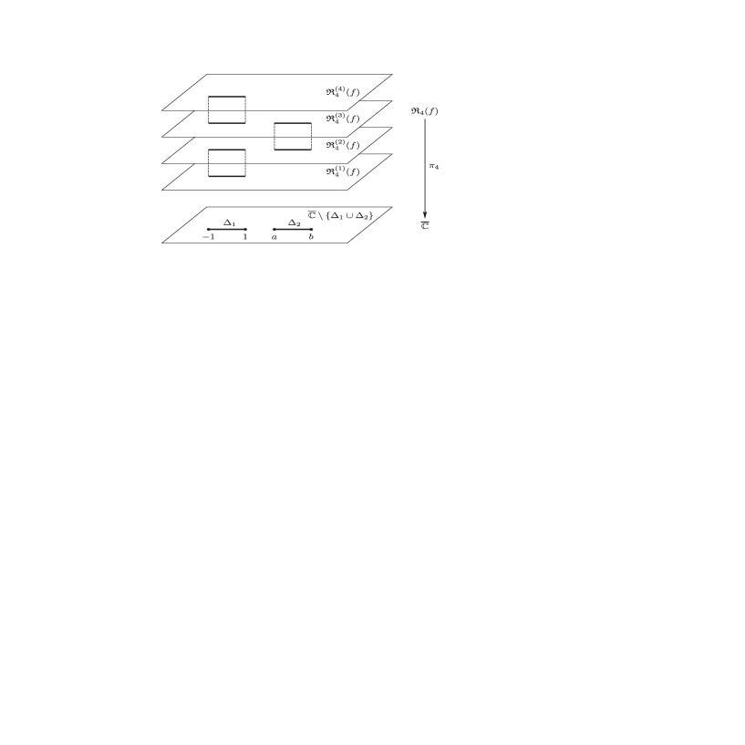
Figure 1: The four-sheeted Riemann surface $\mathfrak{R}_{4}(\widetilde{f})$ of the function $\widetilde{f}$ given by (6).

For a function $f$ defined by (6), the Riemann surface $\mathfrak{R}(f)$ of the function $f$ can be looked upon as a four-sheeted covering of the Riemann sphere $\overline{\mathbb{C}}$ with the branch points $z=\pm 1,a,b$. Let $\pi_{4}\colon\mathfrak{R}_{4}\to\overline{\mathbb{C}}$, $\mathfrak{R}_{4}=\mathfrak{R}_{4}(f)$ be the corresponding canonical projection. We shall assume that the R.s. $\mathfrak{R}_{4}(f)$ is realized as follows (see Fig. 1). The first (open) sheet $\mathfrak{R}^{(1)}_{4}$ of the R.s. $\mathfrak{R}_{4}(f)$ is the Riemann sphere cutted along the interval $\Delta_{1}$. The second $\mathfrak{R}^{(2)}_{4}$ and the third $\mathfrak{R}^{(3)}_{4}$ sheets are the Riemann spheres with cuts, respectively, along the intervals $\Delta_{1}$ and $\Delta_{2}$. Further, the fourth sheet $\mathfrak{R}^{(4)}_{4}$ is the Riemann sphere with cut along the interval $\Delta_{2}$. We follow the standard assumption that each cut along the corresponding interval has two ‘‘edges’’ (the upper and bottom ones). The four sheets are ‘‘glued’’ into the surface by the standard crosswise identification of the upper and bottom edges of the corresponding cuts of different sheets. According to this rule, the first sheet is connected to the second one by the cut corresponding to the interval $\Delta_{1}$, after this the second sheet is glued to the third sheet along the cut corresponding to the interval $\Delta_{2}$, and lastly, the third sheet is glued to the fourth sheet along the cut corresponding to the interval $\Delta_{1}$. The genus of the R.s. $\mathfrak{R}_{4}(f)$ thus obtained is zero, which means that this R.s. is topologically equivalent to the Riemann sphere $\overline{\mathbb{C}}$.

The points lying on the sheets $\mathfrak{R}_{4}^{(1)}$, $\mathfrak{R}_{4}^{(2)}$, $\mathfrak{R}_{4}^{(3)}$ and $\mathfrak{R}_{4}^{(4)}$ of this R.s.  will be denoted by $z^{(1)},z^{(2)},z^{(3)}$ and $z^{(4)}$, respectively. We set $\Gamma^{(1,2)}=\partial\mathfrak{R}_{4}^{(1)}\cap\partial\mathfrak{R}_{4}^{(2)}$, $\Gamma^{(2,3)}=\partial\mathfrak{R}_{4}^{(2)}\cap\partial\mathfrak{R}_{4}^{(3)}$, $\Gamma^{(3,4)}=\partial\mathfrak{R}_{4}^{(3)}\cap\partial\mathfrak{R}_{4}^{(4)}$. For a function $f\in\mathscr{Z}$ of the form (6), we have $\pi_{4}(z^{(j)})=z\in D_{1}\setminus\Delta_{2}$, $j=1,2,3,4$, $\pi_{4}(\Gamma^{(1,2)})=\pi_{4}(\Gamma^{(3,4)})=\Delta_{1}$, and $\pi_{4}(\Gamma^{(2,3)})=\Delta_{2}$.

In the above notation, the aforementioned results of Stahl’s theory (see (4)–(5)) for a function $f\in\mathscr{Z}$ defined by (6) can be interpreted as follows:

$$[n/n]_{f_{\infty}}(z) \to f(z^{(1)}),\quad z\in D_{1},$$ (7)

$$\bigl{|}f(z^{(1)})-[n/n]_{f_{\infty}}(z)\bigr{|}^{1/n} \to e^{-2g_{\Delta_{1}}(z,\infty)},\quad z\in D_{1}$$ (8)

as $n\to\infty$; the convergence in (7) and (8) is uniform inside the domain $D_{1}$ (i.e., on compact subsets of $D_{1}$). Note that in (7) and (8) the convergence in capacity can be replaced by the uniform convergence, because a function $f$ of the form (6) is easily seen to be a Markov function; i.e., it can be represented as

$$f(z)=\frac{1}{\sqrt{AB}}+\widehat{\sigma}(z),$$

where

$$\widehat{\sigma}(z):=\int_{-1}^{1}\frac{d\sigma(x)}{z-x}$$

is the Cauchy transform of a measure $\sigma$ supported on the interval $\Delta_{1}$.

Thus, the maximal Stahl domain $D_{1}$ corresponds to the first sheet $\mathfrak{R}_{4}^{(1)}$ of the R.s. $\mathfrak{R}_{4}(f)$, which, as was noted above, is topologically equivalent to the Riemann sphere $\overline{\mathbb{C}}$. On this Riemann sphere the domain corresponding to the first sheet occupies, in a sense, only the fourth part of the sphere. Therefore, the maximality of the Stahl domain should be understood as the maximality related only to diagonal Padé approximants: these rational approximants do not converge on any larger domain. The question of the efficient analytic continuation of a given germ $f_{\infty}$ to the other sheets of the R.s. $\mathfrak{R}_{4}(f)$ is shown to be solvable using rational approximants based on Hermite–Padé polynomials.

Until the end of § 2 we assume that $f\in\mathscr{Z}$ is given by representation (6), $f\in\mathscr{H}(D_{1})$, and $f_{\infty}\in\mathscr{H}(\infty)$ is the corresponding germ defined at the point $z=\infty$.

2.2

For the system of three germs $f_{\infty},f_{\infty}^{2},f_{\infty}^{3}$ and an arbitrary $n\in\mathbb{N}$, we define the type II Hermite–Padé polynomials $Q_{3n},P_{3n,1},P_{3n,2},P_{3n,3}\in\mathbb{P}_{3n}$, $Q_{3n}\not\equiv 0$, by the relations (see [33], [31]):

$$(Q_{3n}f_{\infty}-P_{3n,1})(z) =O\left(\frac{1}{z^{n+1}}\right),\quad z\to\infty,$$ (9)

$$(Q_{3n}f_{\infty}^{2}-P_{3n,2})(z) =O\left(\frac{1}{z^{n+1}}\right),\quad z\to\infty,$$ (10)

$$(Q_{3n}f_{\infty}^{3}-P_{3n,3})(z) =O\left(\frac{1}{z^{n+1}}\right),\quad z\to\infty.$$ (11)

It is easily checked that for the function $f$ defined in (6) the system $f,f^{2},f^{3}$ is a Nikishin system (regarding the definition and properties of Nikishin systems, see [30], [31], [16]). Namely, the following representations hold (see [49]):

$$\begin{gathered}f(z)=\frac{1}{\sqrt{AB}}+\widehat{\sigma}(z),\quad f^{2}(z)=\frac{1}{AB}+\frac{1}{\sqrt{AB}}\widehat{\sigma}(z)-\widehat{s}_{1}(z),\\ f^{3}(z)=\frac{1}{\sqrt{(AB)^{3}}}+\frac{1}{AB}\widehat{\sigma}(z)-\frac{1}{\sqrt{AB}}\widehat{s}_{1}(z)-\widehat{s}_{2}(z),\\ \text{where}\quad s_{1}:=\left\langle\sigma,\sigma_{2}\right\rangle,\quad s_{2}:=\left\langle\sigma,\sigma_{2},\sigma\right\rangle\end{gathered}$$ (12)

(for the notation used in (12), see [19]). Hence, since a Nikishin system is perfect (see [16]), we have $\operatorname{deg}{Q_{3n}}=3n$, $\operatorname{deg}{P_{3n,j}}=3n$, $j=1,2,3$. Therefore, by normalizing the polynomials $Q_{3n}$ all these four polynomials are determined uniquely.

We introduce now the necessary notation.

By $g_{\Delta_{j}}(z,\zeta)$ we shall denote the Green function of the domain $D_{j}=\overline{\mathbb{C}}\setminus\Delta_{j}$, $j=1,2$, with singularity at the point $z=\zeta$. The corresponding Green potential of a measure $\mu$, $\operatorname{supp}\mu\subset\mathbb{C}$, is denoted by $G^{\mu}_{\Delta_{j}}(z)$,

$$G^{\mu}_{\Delta_{j}}(z):=\int g_{\Delta_{j}}(\zeta,z)\,\mu(\zeta),\quad z\in D_{j}.$$

By $M_{1}(\Delta_{j})$ we denote the space of all unit (positive Borel) measures with support on $\Delta_{j}$, $j=1,2$. Further, $\beta_{\Delta_{j}}(\mu)$ denotes the balayage of an arbitrary measure $\mu$ from the domain $D_{j}$ onto its boundary $\Delta_{j}=\partial D_{j}$.

Lemma 1.

In the class $M_{1}(\Delta_{2})$, there exists a unique measure $\lambda$ such that on $\Delta_{2}$

$$V^{\lambda}(x_{2})+G^{\lambda}_{\Delta_{1}}(x_{2})+g_{\Delta_{1}}(x_{2},\infty)\equiv\operatorname{const}=\gamma(\lambda),\quad x_{2}\in\Delta_{2},$$ (13)

with some constant $\gamma=\gamma(\lambda)$.

Relation (13) will be called the equilibrium relation, $\lambda$ is the equilibrium measure, and $\gamma(\lambda)$ is the equilibrium constant.

Remark 1.

It is worth pointing out that the equilibrium relation (13) holds for the mixed Green-logarithmic potential $V^{\mu}(z)+G^{\mu}_{\Delta_{1}}(z)$ with the external field $\psi(z)=g_{\Delta_{1}}(z,\infty)$; cf. [17], [18], [35], [13].

Let $\lambda_{1}:=\beta_{\Delta_{1}}(\lambda)\in M_{1}(\Delta_{1})$ be the balayage of the measure $\lambda$ from $D_{1}$ onto $\Delta_{1}$,

$$\lambda_{2}:=\frac{1}{3}\bigl{(}2\tau^{\vphantom{p}}_{\Delta_{1}}+\lambda_{1}\bigr{)}\in M_{1}(\Delta_{1})$$ (14)

(recall that $\tau^{\vphantom{p}}_{\Delta_{1}}$ is the Robin measure of the interval $\Delta_{1}$).

The following result holds.

Theorem 1.

The degree of the polynomial $Q_{3n}$ is $3n$, all zeros of the polynomial $Q_{3n}$ are simple and lie in the interval $\Delta_{1}^{\circ}:=(-1,1)$. Moreover, if $n\to\infty$, then

$$\frac{1}{n}\chi(Q_{3n}) \overset{*}{\longrightarrow}3\lambda_{2};$$ (15)

$$\frac{P_{3n,1}}{Q_{3n}}(z) \to f(z^{(1)}),\quad z\in D_{1};$$ (16)

the convergence rate in (16) can be characterized by the relation

$$\biggl{|}f(z^{(1)})-\frac{P_{3n,1}}{Q_{3n}}(z)\biggr{|}^{1/n}\to\delta_{1}(z),\quad z\in D_{1},$$ (17)

where

$$\delta_{1}(z):=e^{-\bigl{(}G^{\lambda}_{\Delta_{1}}(z)+2g_{\Delta_{1}}(z,\infty)\bigr{)}}<1,\quad z\in D_{1}$$

(cf. (7) and (8)). The convergence in (16) and (17) is uniform inside the domain $D_{1}$.

Remark 2.

Note that if $n\to\infty$, then

$$\frac{P_{3n,2}}{Q_{3n}}(z)\to f^{2}(z^{(1)}),\quad\frac{P_{3n,3}}{Q_{3n}}(z)\to f^{3}(z^{(1)}),\quad z\in D_{1}.$$

However, these relations provide no additional information about the values of the function $f(z^{(1)})$ for $z\in D_{1}$.

2.3

For the family of germs $[1,f_{\infty},f_{\infty}^{2},f_{\infty}^{3}]$ and an arbitrary $n\in\mathbb{N}$, the type I Hermite–Padé polynomials $Q_{n,j}\in\mathbb{P}_{n}$, $Q_{n,j}\not\equiv 0$, $j=0,1,2,3$, are defined (not uniquely) by the relation

$$R_{n}(z):=(Q_{n,0}+Q_{n,1}f_{\infty}+Q_{n,2}f_{\infty}^{2}+Q_{n,3}f_{\infty}^{3})(z)=O\left(\frac{1}{z^{3n+3}}\right),\quad z\to\infty$$ (18)

(for more details, see [33], [31]).

The following result holds.

Theorem 2.

For any $n\in\mathbb{N}$ $\operatorname{deg}{Q_{n,j}}=n$, $j=0,1,2,3$. All zeros of the polynomials $Q_{n,j}$ are simple and lie in the interval $\Delta_{1}^{\circ}$. Moreover, if $n\to\infty$, then

$$\frac{1}{n}\chi(Q_{n,j})\overset{*}{\longrightarrow}\lambda_{1}\in M(\Delta_{1}),\quad j=0,1,2,3;$$ (19)

$$\frac{Q_{n,2}}{Q_{n,3}}(z)\to-\bigl{[}f(z^{(1)})+f(z^{(2)})+f(z^{(3)})\bigr{]},\quad z\in D_{1};$$ (20)

the convergence rate in (20) is characterized by the relation

$$\biggl{|}\bigl{[}f(z^{(1)})+f(z^{(2)})+f(z^{(3)})\bigr{]}+\frac{Q_{n,2}}{Q_{n,3}}(z)\biggr{|}^{1/n}\to\delta_{3}(z),\quad z\in D_{1},$$ (21)

where

$$\delta_{3}(z):=e^{-2G^{\lambda}_{\Delta_{1}}(z)}<1,\quad z\in D_{1}$$

(cf. (7) and (8)). The convergence in (20) and (21) is uniform inside the domain $D_{1}$.

Remark 3.

Note that convergence in (20) follows directly from more general results of [25]. The description of the measures $\lambda_{2}$ and $\lambda_{1}$ that characterize the limit distribution of the zeros of the polynomials $Q_{3n}$ and $Q_{n,j}$ in terms of the scalar equilibrium problem (13) seems to be new. Usually such a description is given in terms of the vector equilibrium problem (see, prima facie, [17], [19], and also [3, § 5]). This remark also applies to assertion (15) of Theorem 1 on the limit distribution of the zeros of the type II Hermite–Padé polynomials $Q_{3n}$. Namely, as was pointed out above, the system of functions $f,f^{2},f^{3}$ forms a Nikishin system. In this case, the vector equilibrium problem with the Nikishin interaction matrix (see, above all, [30], and also [31], [19], [3, § 5]) is traditionally used to describe the limit distribution of the zeros of type II Hermite–Padé polynomials. For the system of functions $f,f^{2},f^{3}$ such a matrix is a $3\times 3$-matrix. In contrast to the traditional vector approach, we have succeeded in obtaining a complete characterization of the limit distribution of the zeros of type I and type II Hermite–Padé polynomials in terms of the scalar equilibrium problem (13). It is quite likely that, for an arbitrary Nikishin system consisting of any number of functions, the description of the limit distribution of the zeros of the corresponding Hermite–Padé polynomials can be phrased in terms of an appropriate scalar equilibrium problem. This assumption pertains, of course, only to the diagonal case. The off-diagonal case has some special features (see, for example, [26] and the references given therein).

2.4

In relation (18) it was assumed that $\operatorname{deg}{Q_{n,j}}\leqslant{n}$ for all $j=0,1,2,3$. Following the standard approach (see [33], [31]), we now introduce the three-dimensional multiindices $\mathbf{n}_{1}:=(n,n-1,n-1)$, $\mathbf{n}_{2}:=(n,n,n-1)$, and the corresponding type I Hermite–Padé polynomials $Q_{\mathbf{n}_{1},j}$ and $Q_{\mathbf{n}_{2},j}$, $j=0,1,2,3$.

For the multiindex $\mathbf{n}_{1}$, the polynomials $Q_{\mathbf{n}_{1},0},Q_{\mathbf{n}_{1},1}$ lie in $\mathbb{P}_{n}^{*}$, the polynomials $Q_{\mathbf{n}_{1},2},Q_{\mathbf{n}_{1},3}$ lie in $\mathbb{P}_{n-1}^{*}$, and moreover (see (13)),

$$R_{\mathbf{n}_{1}}(z):=(Q_{\mathbf{n}_{1},0}+Q_{\mathbf{n}_{1},1}f_{\infty}+Q_{\mathbf{n}_{1},2}f_{\infty}^{2}+Q_{\mathbf{n}_{1},3}f_{\infty}^{3})(z)=O\left(\frac{1}{z^{3n+1}}\right),\quad z\to\infty,$$ (22)

$\operatorname{deg}{Q_{\mathbf{n}_{1},0}}=\operatorname{deg}{Q_{\mathbf{n}_{1},1}}=n$, $\operatorname{deg}{Q_{\mathbf{n}_{1},2}}=\operatorname{deg}{Q_{\mathbf{n}_{1},3}}=n-1$, all zeros of the polynomials $Q_{\mathbf{n}_{1},j}$, $j=0,1,2,3$, are simple and lie in the interval $\Delta_{1}^{\circ}$.

For the multiindex $\mathbf{n}_{2}$, the polynomials $Q_{\mathbf{n}_{2},0},Q_{\mathbf{n}_{2},1},Q_{\mathbf{n}_{2},2}$ lie in $\mathbb{P}_{n}^{*}$, the polynomial $Q_{\mathbf{n}_{2},3}$ lies in $\mathbb{P}_{n-1}^{*}$, and moreover,

$$R_{\mathbf{n}_{2}}(z):=(Q_{\mathbf{n}_{2},0}+Q_{\mathbf{n}_{2},1}f_{\infty}+Q_{\mathbf{n}_{2},2}f_{\infty}^{2}+Q_{\mathbf{n}_{2},3}f_{\infty}^{3})(z)=O\left(\frac{1}{z^{3n+2}}\right),\quad z\to\infty,$$ (23)

$\operatorname{deg}{Q_{\mathbf{n}_{2},0}}=\operatorname{deg}{Q_{\mathbf{n}_{2},1}}=\operatorname{deg}{Q_{\mathbf{n}_{2},2}}=n$, $\operatorname{deg}{Q_{\mathbf{n}_{2},3}}=n-1$, all zeros of the polynomials $Q_{\mathbf{n}_{2},j}$, $j=0,1,2,3$, are simple and lie in the interval $\Delta_{1}^{\circ}$.

We now set

$$S_{2n,1}(z): =\begin{vmatrix}Q_{\mathbf{n}_{1},1}(z)&Q_{\mathbf{n}_{1},3}(z)\\ Q_{\mathbf{n}_{2},1}(z)&Q_{\mathbf{n}_{2},3}(z)\end{vmatrix}=\bigl{(}Q_{\mathbf{n}_{1},1}Q_{\mathbf{n}_{2},3}-Q_{\mathbf{n}_{1},3}Q_{\mathbf{n}_{2},1}\bigr{)}(z)\in\mathbb{P}_{2n-1},$$ (24)

$$S_{2n,2}(z): =\begin{vmatrix}Q_{\mathbf{n}_{1},2}(z)&Q_{\mathbf{n}_{1},3}(z)\\ Q_{\mathbf{n}_{2},2}(z)&Q_{\mathbf{n}_{2},3}(z)\end{vmatrix}=\bigl{(}Q_{\mathbf{n}_{1},2}Q_{\mathbf{n}_{2},3}-Q_{\mathbf{n}_{1},3}Q_{\mathbf{n}_{2},2}\bigr{)}(z)\in\mathbb{P}_{2n-1}.$$

The following result holds.

Theorem 3.

The interval $\Delta_{2}$ attracts as $n\to\infty$ all zeros of the polynomials $S_{2n,j}$, $j=1,2$, and moreover,

$$\frac{1}{2n}\chi(S_{2n,j}) \overset{*}{\longrightarrow}\lambda\in M_{1}(\Delta_{2});$$ (25)

$$\frac{S_{2n,1}}{S_{2n,2}}(z) \overset{\operatorname{cap}}{\longrightarrow}-\bigl{[}f(z^{(1)})+f(z^{(2)})\bigr{]},\quad z\in D_{2}=\overline{\mathbb{C}}\setminus\Delta_{2};$$ (26)

the convergence rate in (26) can be characterized by the relation

$$\biggl{|}\bigl{[}f(z^{(1)})+f(z^{(2)})\bigr{]}+\frac{S_{2n,1}}{S_{2n,2}}(z)\biggr{|}^{1/n}\overset{\operatorname{cap}}{\longrightarrow}\delta_{2}(z),\quad z\in D_{2},$$ (27)

where

$$\delta_{2}(z):=e^{2\left(V^{\lambda}(z)+G^{\lambda}_{\Delta_{1}}(z)+g_{\Delta_{1}}(z,\infty)-\gamma(\lambda)\right)}<1,\quad z\in D_{2}.$$

Note that in (26)–(27) we assert the convergence in capacity, rather than the uniform convergence as in (16)–(17) and (20)–(21). However, this constraint, which depends only on our method of the proof of Theorem 3, is not related to the essence of the matter, The crux here is that, although various extensions of Hermite–Padé polynomials are well-known (see [40], [15]), it seems that the polynomials $S_{2n,j}$ were not considered earlier and their properties have not been not studied. Relations (24) are explicit representations of the polynomials $S_{2n,j}$ in terms of type I Hermite–Padé polynomials corresponding to two neighbouring multiindices. There is a natural formal definition of these polynomials which is quite similar to the definitions (9)–(11) and (18) of type I and II Hermite–Padé polynomials, respectively. Such definition will be given in the paper [49]. From this definition and the above Theorem 3 it follows that the polynomials $S_{2n,j}$ are intermediate between the type I Hermite–Padé polynomials and the type II Hermite–Padé polynomials.

For a meaningful definition of the polynomials $S_{2n,1}$ and $S_{2n,2}$ in terms of determinants (24), whose entries are type I Hermite–Padé polynomials, it is necessary that these determinants be not identically zero. To satisfy this requirement, the multiindices $\mathbf{n}_{1}$ and $\mathbf{n}_{2}$ should obey a condition more restrictive than the normality condition for the standard PA. In case of (6) (i.e., for real $A$ and $B$), this condition is satisfied. However, in a more general setting with complex $A$ and $B$, this condition ceases to be true (see § 3 below).

In this connection, we recall the following well-known fact (see [33], [31]).

Consider the multiindices $\mathbf{n}_{1}^{\prime}=(n,n-1,n-1)$, $\mathbf{n}_{2}^{\prime}=(n-1,n,n-1)$ and $\mathbf{n}_{3}^{\prime}=(n-1,n-1,n)$ (the multiindex $\mathbf{n}_{1}^{\prime}$ coincides with the above multiindex $\mathbf{n}_{1}$). Let $Q_{\mathbf{n}_{k}^{\prime},j}$, $j=0,1,2,3$, $k=1,2,3$, be the corresponding type I Hermite–Padé polynomials. Then we have the following explicit representations for the type II Hermite–Padé polynomials defined by relations (9)–(11)

$$Q_{3n}(z) =\begin{vmatrix}Q_{\mathbf{n}_{1}^{\prime},1}(z)&Q_{\mathbf{n}_{1}^{\prime},2}(z)&Q_{\mathbf{n}_{1}^{\prime},3}(z)\\ Q_{\mathbf{n}_{2}^{\prime},1}(z)&Q_{\mathbf{n}_{2}^{\prime},2}(z)&Q_{\mathbf{n}_{2}^{\prime},3}(z)\\ Q_{\mathbf{n}_{3}^{\prime},1}(z)&Q_{\mathbf{n}_{3}^{\prime},2}(z)&Q_{\mathbf{n}_{3}^{\prime},3}(z)\end{vmatrix},$$ (28)

$$P_{3n,1}(z) =-\begin{vmatrix}Q_{\mathbf{n}_{1}^{\prime},0}(z)&Q_{\mathbf{n}_{1}^{\prime},2}(z)&Q_{\mathbf{n}_{1}^{\prime},3}(z)\\ Q_{\mathbf{n}_{2}^{\prime},0}(z)&Q_{\mathbf{n}_{2}^{\prime},2}(z)&Q_{\mathbf{n}_{2}^{\prime},3}(z)\\ Q_{\mathbf{n}_{3}^{\prime},0}(z)&Q_{\mathbf{n}_{3}^{\prime},2}(z)&Q_{\mathbf{n}_{3}^{\prime},3}(z)\end{vmatrix}$$

under the assumption that the determinants do not vanish identically. Similar representations under the same nondegeneracy conditions also hold for the polynomials $P_{3n,2}$ and $P_{3n,3}$.

We emphasize once again that definition (9)–(11) of a type II Hermite–Padé polynomials is much more general than the explicit representation (28). Namely, according to (9)–(11) such polynomials $Q_{3n}\not\equiv 0$, $P_{3n,j}\not\equiv 0$ always exist, whereas representation (28) does not always hold. The situation with the above polynomials $S_{2n,j}$ is quite similar. As was already mentioned above, we plan to discuss these polynomials in detail in the separate paper [49]. Nevertheless, we mention however that from the above it follows that the type I Hermite–Padé polynomials themselves play in a sense a key role in the efficient solution of the problem of analytic continuation of a given germ of a multivalued analytic function. Indeed, all rational approximants involved in this procedure can in principle be calculated in terms of such polynomials corresponding to various multiindices.

2.5

Thus, relations (16), (26) and (20) collectively compose the set from which one can recover in succession, from local data (a germ $f_{\infty}$), the values of a multivalued function $f(z)$ on the first, second, and third sheets of the R.s. $\mathfrak{R}_{4}(f)$. Of course, here we speak about the limit procedure, in which, for a given germ $f_{\infty}\in\mathscr{H}(\infty)$, the number of Laurent coefficients involved in the construction of appropriate rational approximants grows unboundedly, because an analytic function cannot be given by a finite number of its Laurent coefficients. Note that for each $n\in\mathbb{N}$ the number of Laurent coefficients involved in the construction of the three functions under consideration is at most $3n+4$.

It is also worth pointing out that $f(z)$ cannot be extended to the last fourth sheet $\mathfrak{R}^{(4)}_{4}$ of the R.s. $\mathfrak{R}_{4}(f)$ by the above procedure. This is in full accord with the fact that the diagonal Padé approximants extend the germ $w_{\infty}\in\mathscr{H}(\infty)$ of the hyperelliptic function $w$, $w^{2}=P_{2\ell}(z)=z^{2\ell}+\dotsb\in\mathbb{P}_{2\ell}$, only on the first sheet of the corresponding two-sheeted hyperelliptic surface. This seems to be quite natural, because, in simple terms, the values of the hyperelliptic function $w$ differ on two sheets of the corresponding R.s. only by the sign.

We also emphasize the following fact. The reader may well have formed the impression that on the first sheet $\mathfrak{R}^{(1)}_{4}$ of the R.s. $\mathfrak{R}_{4}(f)$ the function $f$ can be always recovered from the germ $f_{\infty}$ using the diagonal PA $[n/n]_{f_{\infty}}$. But this is not so. The thing is that when speaking about the partition of the R.s. $\mathfrak{R}_{4}(f)$ into ‘‘sheets’’ we have tacitly meant an intuitive (but never formalized) perception about the sheets of the R.s. $\mathfrak{R}_{4}(f)$ based on the cuts drawn along the already specified intervals $\Delta_{1}=[-1,1]$ and $\Delta_{2}=[a,b]$. But in the general case, even for a simple function of the form (6), this is no longer the case and the thing is more complicated. Namely, the situation changes drastically if at least one of the two points $a=(A+1/A)/2$ or $b=(B+1/B)/2$ moves from the real line into the complex plane: the natural (for the Hermite–Padé polynomials) partition of the R.s. $\mathfrak{R}_{4}(f)$ into sheets will proceed not along the original intervals $\Delta_{1}$ and $\Delta_{2}$, but along some arcs $\ell_{1}$ and $\ell_{2}$ that joint the points $-1,1$ and $a,b$, respectively. More precisely, here we speak about the so-called canonical or the Nuttall partition of the R.s. into sheets, which is uniquely determined by the real part of some Abelian integral with logarithmic singularities and purely imaginary periods (see [33, Sect. 3], [25, formula (3) and Lemma 5], and also § 3 below). In particular, for such partition into sheets, to the first sheet there corresponds a domain $\overline{\mathbb{C}}\setminus\ell_{1}$, which in general is distinct from the domain $D_{1}=\overline{\mathbb{C}}\setminus\Delta_{1}$ corresponding to the first sheet of the Stahl surface.

It can be shown that in the case when the quantities $A$ and $B$ in (6) are real, the Nuttall partition of the R.s. $\mathfrak{R}_{4}(f)$ into sheets is in accord with the intuitive perception about this partition.

Indeed, it can be easily shown that the real function $u$,

$$u(z^{(1)}): =3V^{\lambda_{2}}(z)\quad z\in D_{1},$$ (29)

$$u(z^{(2)}): =2V^{\lambda}(z)-3V^{\lambda_{2}}(z)+2c_{1},\quad z\in\overline{\mathbb{C}}\setminus(\Delta_{1}\cup\Delta_{2}),$$

$$u(z^{(3)}): =V^{\lambda_{1}}(z)-2V^{\lambda}(z)+2c_{1}+c_{2},\quad z\in\overline{\mathbb{C}}\setminus(\Delta_{1}\cup\Delta_{2}),$$

$$u(z^{(4)}): =-V^{\lambda_{1}}(z)+2c_{1}+c_{2}+2c_{3},\quad z\in D_{1},$$

which is defined in terms of the above (see (13) and (14)) measures $\lambda$, $\lambda_{1}$ and $\lambda_{2}$, where $c_{1},c_{2},c_{3}$ are appropriately chosen constants, is a (singlevalued) harmonic function on the R.s. $\mathfrak{R}_{4}(f)$ everywhere except the four points $\pi_{4}^{-1}(\infty)$ at which it has logarithmic singularities:

$$u(z^{(1)}) =-3\log|z|+O(1),\quad z\to\infty,$$

$$u(z^{(j)}) =\log|z|+O(1),\quad z\to\infty,\quad j=2,3,4.$$

Moreover,

$$u(z^{(1)})<u(z^{(2)})<u(z^{(3)})<u(z^{(4)}),\quad z\in\overline{\mathbb{C}}\setminus(\Delta_{1}\cup\Delta_{2}).$$ (30)

But inequalities (30) mean that our adopted (on an intuitive level) partition of the R.s. $\mathfrak{R}_{4}(f)$ into sheets is in fact the Nuttall partition [33, Sect. 3, relation (3.1.3)]; see also [1], [29] and Fig. 1.

The next section will be dedicated to the complex case – in this setting the dominant role is now played the Nuttall partition of the R.s. $\mathfrak{R}_{4}(f)$ into sheets. The properties of this partition in the complex case are far from being evident [33, Sect. 3], [25, Lemma 5].

3 The complex case

3.1

In this section, we formulate and discuss some theoretical results which we have obtained in the case when in (1) all exponents $\alpha_{j}$ are equal to $\pm 1/2$ and $m$ is an even number. The complex quantities $A_{j}$ are subject to no other constraints than the condition that they are pairwise distinct and $|A_{j}|>1$ for any $j$. In this setting, for such functions $f$ from the class $\mathscr{Z}$ with the four-sheeted R.s., we shall establish some properties of the Nuttall partition of this R.s. $\mathfrak{R}_{4}(f)$; such properties do not hold in a general case. Moreover, in this particular case, our alternative approach to the characterization of the Nuttall partition of the R.s. $\mathfrak{R}_{4}(f)$ into sheets is capable of delivering some additional information about the properties of such a partition.

In the case $m=2$ (under the same conditions on the exponents $\alpha_{1,2}=\pm 1/2$) we shall formulate analogues of Theorems 1–3, which hold, in contrast to the real case, under some additional assumptions on the remainder functions $R_{\mathbf{n}_{1}}$, $R_{\mathbf{n}_{2}}$, and $R_{\mathbf{n}_{3}}$. It should be noted that these constrains on the remainder functions are not related to the essence of the matter, but are rather due to the imperfection of the currently available methods of dealing with asymptotical properties of the Hermite–Padé polynomials. In particular, many conjectures in this direction (see [33], [41], [2]) remain unjustified at present.

First fairly general results on the convergence (in capacity) of diagonal PA were obtained by Nuttall (see [32], [33]) in the class of hyperelliptic functions (in particular, these are the functions whose branch points are only of the second order). It is in this case in which in the early 1980s (i.e., before Stahl’s works of 1985–1986) the Nuttall partition of the hyperelliptic surface $\mathfrak{R}_{2}(w)$ into sheets was introduced using the real part of an Abelian integral of the third kind with purely imaginary periods and appropriate logarithmic singularities at the two points $\pi^{-1}_{2}(\infty)$ (see also (33) and (34)). In this particular case, each of the two Nuttall sheets is a domain. In 1984 Nuttall [33, Sect. 3] put forward the conjecture that for any $m\geqslant 3$ and for the partition of an $m$-sheeted R.s. into Nuttall sheets, the complement of the closure of the last ‘‘uppermost’’ (cf. (30)) sheet is a domain on the original R.s. $\mathfrak{R}_{m}$. In its complete form this conjecture was proved very recently (see Lemma 5 of [25]). In the present paper, for the above class of multivalued analytic functions of the form (1), we prove, under the condition $\alpha_{j}=\pm 1/2$, some additional properties of such a partition; in particular, we show that the first sheet $\mathfrak{R}^{(1)}_{4}(f)$ is connected.

3.2

So, let

$$f(z):=\prod_{j=1}^{m}\left(A_{j}-\frac{1}{\varphi(z)}\right)^{\alpha_{j}},\quad z\in D_{1},$$ (31)

where $\alpha_{j}=\pm 1/2$ for any $j$, $m=0\pmod{2}$, all $A_{j}$ are pairwise distinct, and $|A_{j}|>1$. The class of such functions will be denoted by $\mathscr{Z}_{1/2}$.

Consider the two-sheeted R.s. $\mathfrak{R}_{2}(w)$ of the function $w$ defined by the equality $w^{2}=z^{2}-1$. We shall assume that the R.s. $\mathfrak{R}_{2}(w)$ is realized as a two-sheeted covering of the Riemann sphere $\overline{\mathbb{C}}$ using the explicitly given uniformization

$$z=\frac{1}{2}\left(\zeta+\frac{1}{\zeta}\right),\quad w=\frac{1}{2}\left(\zeta-\frac{1}{\zeta}\right),\quad\zeta\in\overline{\mathbb{C}}_{\zeta}.$$ (32)

Accordingly, the first sheet $\mathfrak{R}^{(1)}_{2}$, on which $w=(z^{2}-1)^{1/2}/z\to 1$ as $z\to\infty$, corresponds to the exterior $\{\zeta:|\zeta|>1\}$ of the unit disc $\mathbb{D}_{\zeta}:=\{\zeta:|\zeta|<1\}$ in the $\zeta$-plane, and the second sheet $\mathfrak{R}^{(2)}_{2}$, on which $w=-(z^{2}-1)^{1/2}/z\to-1$ as $z\to\infty$, corresponds to the unit disc itself. By a point $\mathbf{z}$ on the R.s. $\mathfrak{R}_{2}(w)$, $\mathbf{z}\in\mathfrak{R}_{2}(w)$, we shall mean the pair $\mathbf{z}:=(z,w)=(z,\pm(z^{2}-1)^{1/2})$. The canonical projection $\pi_{2}\colon\mathfrak{R}_{2}(w)\to\overline{\mathbb{C}}$ is defined by $\pi_{2}(\mathbf{z}):=z$. By the point $\mathbf{z}=\infty^{(1)}\in\mathfrak{R}_{2}(w)$ we mean the point on the R.s. $\mathfrak{R}_{2}(w)$ such that $\pi_{2}(\infty^{(1)})=\infty$ and $w/z\to 1$ as $\mathbf{z}\to\infty^{(1)}$. Similarly, for $\mathbf{z}=\infty^{(2)}$ we have $\pi(\infty^{(2)})=\infty$ and $w/z\to-1$ as $\mathbf{z}\to\infty^{(2)}$. A passage from the first sheet $\mathfrak{R}^{(1)}_{2}$ to the second sheet $\mathfrak{R}^{(2)}_{2}$ proceeds along the cut interval $\Delta_{1}$ (here we assume as usual that an interval has two edges, the upper and bottom ones) and that the sheets are ‘‘glued’’ by identifying crosswisely the edges of cuts; i.e., by identifying the upper edge of one cut with the lower edge of the other, and vice versa. It can be easily shown that the above partition into sheets is a Nuttall partition. Indeed, let

$$G(\mathbf{z}):=\int_{-1}^{\mathbf{z}}\frac{dt}{\sqrt{t^{2}-1}}=\log(z+w)=\log(z\pm(z^{2}-1)^{1/2})$$ (33)

be an Abelian integral of the third kind with purely imaginary periods and logarithmic singularities only at the points $\mathbf{z}=\infty{(1)},\infty^{(2)}$. Then $u_{2}(\mathbf{z}):=-\operatorname{Re}G(\mathbf{z})$ is a harmonic function on the R.s. $\mathfrak{R}_{2}(w)\setminus\{\infty^{(1)},\infty^{(2)}\}$,

$$u_{2}(\mathbf{z})=\mp\log|z|+O(1),\quad\mathbf{z}\to\infty^{(1)},{\infty^{(2)}},$$

and

$$u_{2}(z^{(1)})<u_{2}(z^{(2)}),\quad z\in D_{1}.$$ (34)

Moreover, $u_{2}(\mathbf{z})=0$ for $\mathbf{z}\in\boldsymbol{\Gamma}$, $\boldsymbol{\Gamma}:=\pi^{-1}_{2}(\Delta_{1})$. So, $-u_{2}(z^{(1)})=g_{\Delta_{1}}(z,\infty)$ is the Green function of the domain $D_{1}$. An arbitrary germ $f_{\infty}\in\mathscr{H}(\infty)$ of the function $f\in\mathscr{Z}_{1/2}$, $f\in\mathscr{H}(D_{1})$, is lifted to the point $\mathbf{z}=\infty^{(1)}\in\mathfrak{R}_{2}(w)$ and extends to the entire first sheet $\mathfrak{R}^{(1)}_{2}(w)$ as a singlevalued holomorphic function (recall that $\pi_{2}(\mathfrak{R}_{2}^{(1)}(w))=D_{1}=\overline{\mathbb{C}}\setminus\Delta_{1}$). A further singlevalued extension of this function to the entire second sheet of the R.s. $\mathfrak{R}_{2}(w)$ is hindered by the branch points $a^{(2)}_{j}\in\mathfrak{R}^{(2)}_{2}(w)$ such that $\pi_{2}(a^{(2)}_{j})=a_{j}$, $j=1,\dots,m$. In order that such a singlevalued analytic (meromorphic) extension of the germ $f_{\infty}$ be possible one should make appropriate cuts on the second sheet $\mathfrak{R}_{2}^{(2)}(w)$.

Definition 1 ((cf. [45], Definition 2)).

A compact set $\mathbf{K}=K^{(2)}\subset\mathfrak{R}_{2}^{(2)}(w)$ is called admissible for a germ $f_{\infty}\in\mathscr{H}(\infty^{(1)})$ of a function $f\in\mathscr{Z}_{1/2}$ if this germ $f_{\infty}$ extends as a singlevalued meromorphic function to the domain $\Omega_{\infty^{(1)}}(K^{(2)})$, which is the connected component of the complement of $K^{(2)}$ containing the point $\mathbf{z}=\infty^{(1)}$, $f_{\infty}\in\mathscr{M}(\Omega_{\infty^{(1)}}(K^{(2)}))$.

The class of all admissible compact sets for a germ $f_{\infty}$ will be denoted by $\mathfrak{K}(f_{\infty})$.

Note that one can slightly reduce the class of admissible compact sets and consider a priori only compact sets with connected complement; i.e., such that $\Omega_{\infty^{(1)}}(K^{(2)})=\mathfrak{R}_{2}(w)\setminus K^{(2)}$. This change has not effect on subsequent considerations. In what follows, we shall assume that the family $\mathfrak{K}(f_{\infty})$ consists of only regular compact sets in the sense that the domain $\Omega_{\infty^{(1)}}(K^{(2)})$ is regular with respect to the solution of the Dirichlet problem (see [38], [14]).

We fix a local coordinate $\zeta$ at the point $\mathbf{z}=\infty^{(1)}$, $\zeta(\infty^{(1)})=0$. For an arbitrary compact set $\mathbf{K}\in\mathfrak{K}(f_{\infty})$, consider the Green function $g_{\mathbf{K}}(\mathbf{z},\infty^{(1)})$ of the domain $\Omega_{(1)}(\mathbf{K})$ with logarithmic singularity at the point $\mathbf{z}=\infty^{(1)}$ with due account of the choice of the local coordinate at this point; i.e., by definition $g_{\mathbf{K}}(\mathbf{z},\infty^{(1)})=0$ for $\mathbf{z}\in\partial\Omega_{\infty^{(1)}}(\mathbf{K})$ and

$$g_{\mathbf{K}}(\mathbf{z},\infty^{(1)})=\log\frac{1}{|\zeta|}+\gamma+o(1),\quad\mathbf{z}\to\infty^{(1)},$$ (35)

where $\gamma=\gamma(\mathbf{K})$ is the Robin constant for the domain $\Omega_{\infty(1)}(\mathbf{K})$ at the point $\mathbf{z}=\infty^{(1)}$ with respect to the chosen local coordinate $\zeta$ (see [38, Ch. 8, § 4]).

The following lemma follows from general results of [38].

Lemma 2.

The class $\mathfrak{K}(f_{\infty})$ contains a unique compact set $\mathbf{F}$ such that

$$\gamma(\mathbf{F})=\max_{\mathbf{K}\in\mathfrak{K}(f_{\infty})}\gamma(\mathbf{K}).$$ (36)

This extremal compact set $\mathbf{F}$ does not split the R.s. $\mathfrak{R}_{2}(w)$ (i.e., $\Omega^{(1)}(\mathbf{F})=\mathfrak{R}_{2}(w)\setminus\mathbf{F}$ is a domain), consists of a finite number of analytic arcs, and has the following $S$-property:

$$\frac{\partial g_{\mathbf{F}}(\mathbf{z},\infty^{(1)})}{\partial n^{+}}=\frac{\partial g_{\mathbf{F}}(\mathbf{z},\infty^{(1)})}{\partial n^{-}},\quad\mathbf{z}\in\mathbf{F}^{\circ};$$ (37)

here $\mathbf{F}^{\circ}$ is the union of open arcs whose closures constitute $\mathbf{F}$, $\partial/{\partial n^{+}}$ and $\partial/{\partial n^{-}}$ are the normal derivatives to $\mathbf{F}^{\circ}$ at the point $\mathbf{z}$ taken in opposite directions to the sides of $\mathbf{F}$ (the validity of (37) does not depend on the local coordinate chosen at the point $\mathbf{z}\in\mathbf{F}^{\circ}$).

Lemma 2 is proved using Schiffer’s method of interior variations in accordance with the general idea proposed in [38, Ch. 8, § 4].

The quantity $e^{-\gamma(\mathbf{K})}$ is naturally called the capacity of a compact set $\mathbf{K}$ (this quantity depends on the local coordinate chosen at the point $\mathbf{z}=\infty^{(1)}$). So, $\mathbf{F}\in\mathfrak{K}(f_{\infty})$ is an admissible compact set of minimal capacity (this property is already independent of the choice of a local coordinate).

In the actual fact, the genus of the R.s. $\mathfrak{R}_{2}(w)$ is zero, and hence Lemma 2 can be reduced to the planar case and the corresponding compact set of minimal capacity on the plane. Indeed, a uniformization of $\mathfrak{R}_{2}(w)$ is defined using the Zhukovskii function as follows:

$$z=\frac{1}{2}\left(\zeta+\frac{1}{\zeta}\right),\quad w=\frac{1}{2}\left(\zeta-\frac{1}{\zeta}\right),\quad\zeta\in\overline{\mathbb{C}}_{\zeta}.$$ (38)

To the first sheet of $\mathfrak{R}^{(1)}_{2}(w)$ there corresponds the exterior $\overline{\mathbb{C}}\setminus\overline{\mathbb{D}}$ of the unit disc $\mathbb{D}:=\{\zeta:|\zeta|<1\}$, while the second sheet is the unit disc $\mathbb{D}$. The function $f(z)\in\mathscr{Z}_{1/2}$ of the form (31) is transformed to the function $\widetilde{f}(\zeta)$ of the form

$$\widetilde{f}(\zeta)=\prod_{j=1}^{m}\left(A_{j}-\frac{1}{z+w}\right)^{\alpha_{j}}=\prod_{j=1}^{m}\left(A_{j}-\frac{1}{\zeta}\right)^{\alpha_{j}},$$ (39)

where all $\alpha_{j}=\pm 1/2$. All $A_{j}\in\overline{\mathbb{C}}\setminus\overline{\mathbb{D}}$, and hence all singular points of the function $\widetilde{f}$ are of the form $\zeta=\widetilde{a}_{j}=1/A_{j}\in\mathbb{D}$. So, to the extremal compact set $\mathbf{F}$ for the function $f$ on the R.s. $\mathfrak{R}_{2}(w)$ there corresponds an admissible compact set of minimal capacity $\widetilde{F}$ for the function $\widetilde{f}$, as given by the element $\widetilde{f}_{\infty}\in\mathscr{H}(\infty)$ (note that $\widetilde{f}\in\mathscr{M}(\overline{\mathbb{C}}\setminus\widetilde{F})$ and at the point $\zeta=0$ the function $\widetilde{f}$ has a pole). By well-known properties of a compact set of minimal capacity, $\widetilde{F}\subset\mathbb{D}$ (or, more precisely, the compact set $\widetilde{F}$ lies in the convex hull of the set $\{\widetilde{a}_{j}=1/A_{j}$, $j=1,\dots,m\}$), $\widetilde{F}$ consists of a finite number of analytic arcs (trajectories of quadratic differentials), $\widetilde{F}$ does not split the complex plane and has the $S$-property (37). Moreover,

$$\widetilde{F}=\biggl{\{}\zeta\in\mathbb{C}:\operatorname{Re}\int_{\widetilde{a}_{j}}^{\zeta}\sqrt{\frac{V_{m-2}(t)}{A_{m}(t)}}\,dt=0\biggr{\}},$$ (40)

where $A_{m}(t):=\prod_{j=1}^{m}(t-\widetilde{a}_{j})$, $V_{m-2}(t):=(t-v_{1})\dots(t-v_{m-2})$ is the corresponding Chebotarev polynomial, $v_{j}$, $j=1,\dots,m$, are points of the Chebotarev compact set $\widetilde{F}$. All these properties of a compact set of minimal capacity are well known in a general case and were obtained by Stahl already in 1985 (see [42], [43], as well as [4] and [44]).

In the case under consideration here, all branch points of the function $\widetilde{f}$ are of the second order. In this setting, the existence and description of a compact set of minimal capacity were proved already by Nuttall [32], [33]. In particular, in the case of general position, all zeros of the polynomial $V_{m-2}$ have even multiplicity, all $v_{j}\neq a_{k}$ for $j=1,\dots,m-2$, $k=1,\dots,m$, and the compact set $\widetilde{F}$ consists of $m/2\in\mathbb{N}$ disjoint analytic arcs that joint pairwisely the points of the set $\{\widetilde{a_{j}},j=1,\dots,m\}$.

Thus, on the second sheet of the R.s. $\mathfrak{R}_{2}(w)$ we have obtained a system of analytic arcs which compose the compact set $\mathbf{F}$, do not split the R.s. $\mathfrak{R}_{2}(w)$, have the $S$-property (37), and are such that $f_{\infty}\in\mathscr{M}(\mathfrak{R}_{2}(w)\setminus{\mathbf{F}})$.

We now proceed as follows. Given $\mathbf{z}\in\mathfrak{R}_{2}(w)\setminus\mathbf{F}$, consider the function

$$u(\mathbf{z}):=-2g_{\mathbf{F}}(\mathbf{z},\infty^{(1)})-g(\mathbf{z}),$$

where $g(\mathbf{z})=\log|z+w|=\log|\zeta|$. The function $v(\mathbf{z})$ is harmonic in the domain $\mathfrak{R}_{2}(w)\setminus\mathbf{F}$ except for the points at infinity $\mathbf{z}=\infty^{(1)}$ and $\mathbf{z}=\infty^{(2)}$, where it behaves as

$$u(\mathbf{z})=\begin{cases}-3\log|z|+O(1),&\mathbf{z}\to\infty^{(1)},\\ \log|z|+O(1),&\mathbf{z}\to\infty^{(2)}\end{cases}$$ (41)

(here and in what follows we assume for simplicity that $\infty^{(2)}\not\in\mathbf{F}$; otherwise a more accurate analysis is required quite similar to that of [25]).

We set

$$\mathbf{E}:=\bigl{\{}\mathbf{z}\in\mathfrak{R}_{2}(w):u(z^{(1)})=u(z^{(2)})\bigr{\}};$$ (42)

here by $z^{(1)}\in\mathfrak{R}^{(1)}_{2}(w)$ and $z^{(2)}\in\mathfrak{R}^{(2)}_{2}(w)$ we mean, as before, the Nuttall partition of the R.s. $\mathfrak{R}_{2}(w)$ into sheets. It is easily checked that $\mathbf{E}$ is a closed arc on the R.s. $\mathfrak{R}_{2}(w)$ passing through the points $\mathbf{z}=\pm 1$, not crossing the compact set $\mathbf{F}$, and splitting $\mathfrak{R}_{2}(w)$ into two domains, of which one contains $\mathbf{F}$, and the other one, the point $\mathbf{z}=\infty^{(1)}$. Let us now take the second copy of the R.s. $\mathfrak{R}_{2}(w)$ (which we denote by $\mathfrak{R}_{2}^{\prime}(w)$) with cuts drawn along the arcs of the compact set $\mathbf{F}$, and glue it to the first copy with the same cuts using the standard crosswise identification of the opposite edges of a cut. This gives us a four-sheeted R.s. on which the original germ $f_{\infty}\in\mathscr{H}(\infty^{(1)})$ extends as a singlevalued meromorphic function, because this four-sheeted R.s. coincides with the R.s. $\mathfrak{R}_{4}(f)$. We have $g_{\mathbf{F}}(\mathbf{z},\infty^{(1)})=0$ for $\mathbf{z}\in\mathbf{F}$, and hence the function $g_{\mathbf{F}}(\mathbf{z},\infty^{(1)})$ extends continuously to the glued R.s. $\mathfrak{R}_{2}^{\prime}(w)$ by continuity with the sign change. The $S$-property (37) guarantees that this extension is a harmonic function on the four-sheeted R.s. thus obtained. The function $g(\mathbf{z})$ is harmonic in a neighbourhood of the compact set $\mathbf{F}$, and hence $f$ extends to the second copy of the R.s. $\mathfrak{R}_{2}(w)$ by duplication of its values from the first copy of $\mathfrak{R}_{2}(w)$. By $\mathbf{E}^{\prime}$ we denote the closed curve lying on the second copy of $\mathfrak{R}_{2}(w)$ and corresponding to the curve $\mathbf{E}$; by $\infty^{(4)}$ we denote the point lying on the second copy of $\mathfrak{R}_{2}(w)$ and corresponding to the point $\mathbf{z}=\infty^{(1)}$.

We now partition the four-sheeted R.s. $\mathfrak{R}_{4}$ thus obtained into sheets as follows. The first sheet $\mathfrak{R}^{(1)}_{4}$ is the domain containing the point $\mathbf{z}=\infty^{(1)}$ with boundary $\partial\mathfrak{R}^{(1)}_{4}=\mathbf{E}$. The second sheet $\mathfrak{R}^{(2)}_{4}$ is the domain with boundary $\mathbf{E}\cup\mathbf{F}$. The third sheet $\mathfrak{R}^{(3)}_{4}$ is the domain with boundary $\mathbf{F}\cup\mathbf{E}^{\prime}$. And the fourth sheet $\mathfrak{R}^{(4)}_{4}$ is the domain with boundary $\mathbf{E}^{\prime}$. Given $\mathbf{z}\in\mathfrak{R}_{2}^{\prime}(w)$, we now set

$$u(\mathbf{z}):=-2g_{\mathbf{F}}(\mathbf{z},\infty^{(1)})-g(\mathbf{z});$$ (43)

the meaning of the functions $g_{\mathbf{F}}(\mathbf{z},\infty^{(1)})$ and $g(\mathbf{z})$ for $\mathbf{z}\in\mathfrak{R}_{2}^{\prime}(w)$ was already explained above. It is easily checked that $u(\mathbf{z})$ is a harmonic function in the domain $\mathfrak{R}_{4}(f)\setminus\{\infty^{(1)},\infty^{(2)},\infty^{(3)},\infty^{(4)}\}$. Moreover,

$$u(\mathbf{z})=\begin{cases}-3\log|z|+O(1),&\mathbf{z}\to\infty^{(1)},\\ \log|z|+O(1),&\mathbf{z}\to\infty^{(2)},\\ \log|z|+O(1),&\mathbf{z}\to\infty^{(3)},\\ \log|z|+O(1),&\mathbf{z}\to\infty^{(4)},\end{cases}$$ (44)

and besides, for the above partition of the R.s. $\mathfrak{R}_{4}(f)$ into sheets,

$$u(z^{(1)})<u(z^{(2)})<u(z^{(3)})<u(z^{(4)}).$$ (45)

So, the partition of the R.s. $\mathfrak{R}_{4}(f)$ into sheets, which we introduced using the Green function $g_{\mathbf{F}}(\mathbf{z},\infty)$ corresponding to the compact set of minimal capacity $\mathbf{F}\subset\mathfrak{R}_{2}(w)$, turned out to be a Nuttall partition; for more details, see [49].

3.3

In the remaining part of the present section we shall content ourselves with the case $m=2$ in representation (31). To be more precise, we shall assume as in § 2 that $f\in\mathscr{Z}$ has the form

$$f(z)=\biggl{[}\left(A-\frac{1}{\varphi(z)}\right)\left(B-\frac{1}{\varphi(z)}\right)\biggr{]}^{-1/2},$$ (46)

where, as before, $|A|>1$, $|B|>1$, but in contrast to § 2, $A$ and $B$ are not supposed to be real.

We fix a germ $f_{\infty}\in\mathscr{H}(\infty)$ of a function $f\in\mathscr{H}(D_{1})$ of the form (46) (two possible germs differ only by the sign). By the original assumption about the inverse of the Zhukovskii function (namely, $|\varphi(z)|>1$ for $z\notin\Delta_{1}$) we have $f_{\infty}\in\mathscr{H}(D_{1})$. We recall that, from the viewpoint of Stahl’s theory, the first sheet of the two-sheeted R.s. associated with the germ $f_{\infty}$ is the first sheet $\mathfrak{R}^{(1)}_{2}(w)\ni z^{(1)}$ of the R.s. $\mathfrak{R}_{2}(w)$ of the function $w^{2}=z^{2}-1$ defined by the inequality (see (34))

$$-g(z^{(1)})<-g(z^{(2)})$$

with the canonical projection $\pi_{2}\colon\mathfrak{R}_{2}(w)\to\overline{\mathbb{C}}$, $\pi_{2}(\mathbf{z})=z$, where $\mathbf{z}=(z,w)$ under the assumption that $w/z\to 1$ for $\mathbf{z}\in\mathfrak{R}^{(1)}_{2}(w)$, $\mathbf{z}\to\infty^{(1)}$, and $w/z\to-1$ for $\mathbf{z}\in\mathfrak{R}^{(2)}_{2}(w)$, $\mathbf{z}\to\infty^{(2)}$.

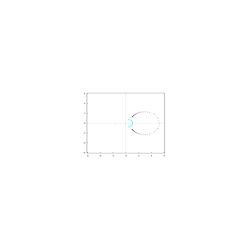
Figure 10: Example 3. The zeros of the type II Hermite–Padé polynomial $Q_{2n}$ (light blue points) for $n=50$ and the zeros (red, dark blue and black points) of the type I Hermite–Padé polynomials $Q_{\mathbf{n},j}$, $j=0,1,2$, for $\mathbf{n}=(50,50)$. From these data and with the help of relations (71) and (72) the structure of the Nuttall partition into sheets of the three-sheeted R.s. $\mathfrak{R}_{3}(w)$ with the germ $\widetilde{f}_{0}$ is analyzed. In accordance with (71), the zeros of the polynomial $Q_{2n}$ model the compact set $E_{2}=\pi_{3}(F^{(1,2)})$ and the zeros of the polynomials $Q_{\mathbf{n},j}$ model the compact set $F_{2}=\pi_{3}(F^{(2,3)})$. Both these compact sets intersect the real line, but, in contrast to Example 2 (Fig. 8), the compact set $F_{2}$ lies to the right of the compact set $E_{2}$.

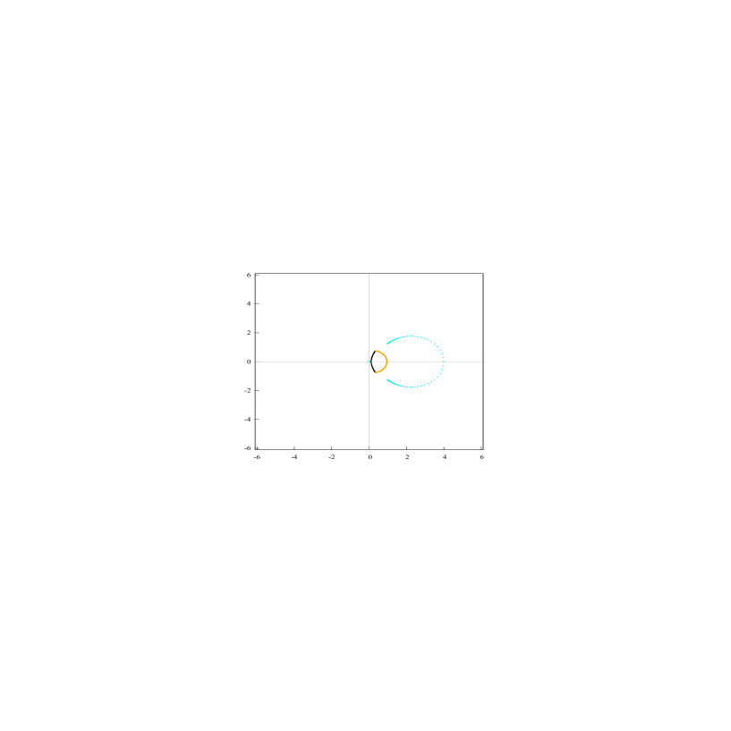
Figure 13: Example 3. The figure combines Figs. 11 and 12. It shows that all three compact sets $E$, $F$ and $E^{\prime}$ intersect the real line between the points $x=0$ and $x=6$. But the compact set $E^{\prime}$ lies to the left of the compact sets $E$ and $F$.

From what has already been said above in § 3.2 of this section it follows that, in the case when at least one of the numbers $A$ or $B$ does not lie on the real line, the Nuttall partition of the R.s. $\mathfrak{R}_{4}(f)$ into sheets proceeds in a nontrivial manner – namely, not along closed curves on $\mathfrak{R}_{4}(f)$ (corresponding, from the viewpoint of the canonical projection $\pi_{4}\colon\mathfrak{R}_{4}(f)\to\overline{\mathbb{C}}$, to the intervals $\Delta_{1}$ and $\Delta_{2}$), but rather along the curves $\mathbf{E}$, $\mathbf{F}$ and $\mathbf{E}^{\prime}$, to which, for a given canonical projection, there correspond some arcs $E$, $F$ and $E^{\prime}$ connecting pairwise the points $-1,1$, $a,b$ and again the point $-1,1$. Correspondingly the first sheet $\mathfrak{R}^{(1)}_{4}$ of the Nuttall partition into sheets of the R.s. $\mathfrak{R}_{4}(f)$ is now different from the first sheet of the Stahl surface $\mathfrak{R}_{2}(w)$ (even though the active branch points $\mathbf{z}=\pm 1$ lying on the boundary of these two sheets are the same). More precisely, we have $\pi_{2}(\mathfrak{R}_{2}^{(1)}(w))=\overline{\mathbb{C}}\setminus\Delta_{1}\neq\overline{\mathbb{C}}\setminus E=\pi_{4}(\mathfrak{R}^{(1)}_{4})$, because in a general case $E\neq\Delta_{1}$. Additionally, as is easily seen from the results of § 3.2, we have $E\cap F=\varnothing$, $F\cap E^{\prime}=\varnothing$ ($E=E^{\prime}$ in the real case). These facts are of uttermost importance in the use of Hermite–Padé polynomials in applications that will be discussed in the concluding § 5 of the present paper (see Figs. 10–13).

Let $R_{\mathbf{n}_{1}},R_{\mathbf{n}_{2}}$ and $R_{\mathbf{n}_{3}}$ be the remainder functions for the three-dimensional multiindexes $\mathbf{n}_{1}:=(n,n-1,n-1)$, $\mathbf{n}_{2}:=(n,n,n-1)$ and $\mathbf{n}_{3}:=(n,n,n)$, respectively (see (22), (23) and (18)). For $A,B\in\mathbb{R}$, all these multiindices are normal (for the definition of a normal multiindex, see [31]). This result is a corollary of the fact of [16] that an arbitrary Nikishin system is perfect (see also [31] and [15]). Therefore, we have as $z\to\infty$

$$R_{\mathbf{n}_{1}}(z)=\frac{C_{\mathbf{n}_{1}}}{z^{3n+1}}+\dots,\quad R_{\mathbf{n}_{2}}(z)=\frac{C_{\mathbf{n}_{2}}}{z^{3n+2}}+\dots,\quad R_{\mathbf{n}_{3}}(z)=\frac{C_{\mathbf{n}_{1}}}{z^{3n+3}}+\dots,$$ (47)

where $C_{\mathbf{n}_{1}},C_{\mathbf{n}_{2}},C_{\mathbf{n}_{3}}\neq 0$. For complex $A$ and $B$ this fact ceases to be true.

All three functions $R_{\mathbf{n}_{1}},R_{\mathbf{n}_{2}}$ and $R_{\mathbf{n}_{3}}$ are (singlevalued) meromorphic functions on the R.s. $\mathfrak{R}_{4}(f)$. One can easily find their divisors (of zeros and poles). Namely, the following explicit representations hold:

$$(R_{\mathbf{n}_{1}}) =(3n+1)\infty^{(1)}-n\infty^{(2)}-n\infty^{(3)}-n\infty^{(4)}-3(\mathbf{a}+\mathbf{b})+\sum_{j=1}^{5}\mathbf{p}_{1,j}(n),$$ (48)

$$(R_{\mathbf{n}_{2}}) =(3n+2)\infty^{(1)}-n\infty^{(2)}-n\infty^{(3)}-n\infty^{(4)}-3(\mathbf{a}+\mathbf{b})+\sum_{j=1}^{4}\mathbf{p}_{2,j}(n),$$

$$(R_{\mathbf{n}_{3}}) =(3n+3)\infty^{(1)}-n\infty^{(2)}-n\infty^{(3)}-n\infty^{(4)}-3(\mathbf{a}+\mathbf{b})+\sum_{j=1}^{3}\mathbf{p}_{3,j}(n).$$

In the real case, since a Nikishin system is perfect, there can be no cancelations (of zeros and poles) in (48); i.e., all $\mathbf{p}_{k,j}(n)\neq\mathbf{a},\mathbf{b}$. Besides, it follows directly from (47) that all $\mathbf{p}_{k,j}(n)\neq\infty^{(1)}$. Moreover, in can be shown that, for any $n\in\mathbb{N}$,

$$\mathbf{p}_{k,j}(n)\in\mathfrak{R}_{4}(f)\setminus\overline{\mathfrak{R}^{(1)}_{4}}.$$ (49)

However, this is not so in the complex case. It might happen that some of the above results also hold in the case of a ‘‘general position’’, but this requires special consideration and as yet remains unjustified. Unfortunately, by now the theory of Hermite–Padé polynomials is not capable of providing meaningful and pretty general results on the asymptotic behaviour of such polynomials in the complex case. Many of particular results obtained in the complex case depend, to a greater or lesser degree, on the possibility of reduction of this particular problem to the real setting (see, for example, [12], [27]). Due to the imperfections of the presently developed methods in the theory of Hermite–Padé polynomials, practically all fairly general and well-known conjectures on the asymptotic behaviour of such polynomials remain unsolved for a long time (for various conjectures in this direction, see [33], [41], [2], and also [36], [37], [48], [47]). It is worth pointing out that the conjecture on topological properties of the canonical partition (presently called the Nuttall partition) of an arbitrary Riemann surface into sheets posed by Nuttall [33, Sect. 3] in 1984 was proved very recently in 2017 in [25].

For the validity of the analogue of Theorem 2 in the complex case considered here, no additional constraints are required, because the required result follows directly from a more general recent result (see Theorem 2 of [25]).

Theorem 4.

Let $Q_{n,j}$, $j=0,1,2,3$, be the Hermite–Padé polynomials defined by (18). Then, for any $j$, the compact set $E^{\prime}=\pi_{4}(\mathbf{E}^{\prime})$ attracts as $n\to\infty$ all zeros of the polynomials $Q_{n,j}$, except possibly a finite number (independent of $n$) of zeros. Moreover,

$$\frac{Q_{n,2}}{Q_{n,3}}(z)\overset{\operatorname{cap}}{\longrightarrow}-\bigl{[}f(z^{(1)})+f(z^{(2)})+f(z^{(3)})\bigr{]},\quad z\in\overline{\mathbb{C}}\setminus E^{\prime}.$$ (50)

Let us now introduce the multiindices $\mathbf{n}_{1}=(n,n-1,n-1)$, $\mathbf{n}_{2}=(n-1,n,n-1)$ and $\mathbf{n}_{3}=(n-1,n-1,n)$. Let $Q_{\mathbf{n}_{k},j}$, $j=0,1,2,3$ be the corresponding type I Hermite–Padé polynomials for the tuple $[1,f_{\infty},f_{\infty}^{2},f_{\infty}^{3}]$, and $R_{\mathbf{n}_{k}}(z)$, $k=1,2,3$, be the corresponding remainder functions

$$R_{\mathbf{n}_{k}}(z)=(Q_{\mathbf{n}_{k},0}+Q_{\mathbf{n}_{k},1}f_{\infty}+Q_{\mathbf{n}_{k},2}f_{\infty}^{2}+Q_{\mathbf{n}_{k},3}f^{3}_{\infty})(z)=O\left(\frac{1}{z^{3n+1}}\right),\quad z\to\infty.$$ (51)

The functions $R_{\mathbf{n}_{k}}$ are singlevalued meromorphic functions on the R.s. $\mathfrak{R}_{4}(f)$, which are completely defined by its divisor,

$$(R_{\mathbf{n}_{k}})=(3n+1)\infty^{(1)}-n\infty^{(2)}-n\infty^{(3)}-n\infty^{(4)}-3(\mathbf{a}+\mathbf{b})+\sum_{j=1}^{5}\mathbf{p}_{k,j}(n).$$ (52)

Given two arbitrary distinct points $\mathbf{z}_{1}$ and $\mathbf{z}_{2}$, $\mathbf{z}_{1},\mathbf{z}_{2}\in\mathfrak{R}_{4}(f)$, we denote by $G(\mathbf{z}_{1},\mathbf{z}_{2};\mathbf{z})$ an Abelian integral of the third kind on the R.s. $\mathfrak{R}_{4}(f)$ with purely imaginary periods and logarithmic singularities only at the points $\mathbf{z}_{1}$ and $\mathbf{z}_{2}$, which in the corresponding local coordinate read as

$$G(\mathbf{z}_{1},\mathbf{z}_{2};\mathbf{z}) =-\log{\zeta}+O(1),\quad\mathbf{z}\to\mathbf{z}_{1},$$ (53)

$$G(\mathbf{z}_{1},\mathbf{z}_{2};\mathbf{z}) =\log{\zeta}+O(1),\quad\mathbf{z}\to\mathbf{z}_{2}.$$

Consequently,

$$\Psi(\mathbf{z}_{1},\mathbf{z}_{2};\mathbf{z}):=\exp\bigl{\{}G(\mathbf{z}_{1},\mathbf{z}_{2};\mathbf{z})\bigr{\}}$$ (54)

is a multivalued analytic function on the R.s. $\mathfrak{R}_{4}(f)$ with singlevalued modulus, a pole at the point $\mathbf{z}=\mathbf{z}_{1}$, and a zero at the point $\mathbf{z}=\mathbf{z}_{2}$. According to (52) and (54), for any $k=1,2,3$ the remainder function $R_{\mathbf{n}_{k}}$ can be written as

$$R_{\mathbf{n}_{k}}=C_{k}\exp\biggl{\{}n\sum\limits_{j=2}^{4}G(\infty^{(j)}),\infty^{(1)};\mathbf{z})+\sum\limits_{j=1}^{5}G(\mathbf{a}_{j},\mathbf{p}_{k,j}(n);\mathbf{z})+G(\mathbf{a}_{6},\infty^{(1)};\mathbf{z})\biggr{\}},$$ (55)

where $C_{1},C_{2},C_{3}\neq 0$ are the normalized constants and for convenience we have denoted the poles of the function $f^{3}$ on the R.s. $\mathfrak{R}_{4}(f)$ by $\{\mathbf{a}_{1},\dots,\mathbf{a}_{6}\}$, where each pole appears as many times as its multiplicity.

To prove analogues of Theorems 2 and 3 we shall require some additional conditions. As was already pointed out, these conditions, which are not related to the essence of the matter, appear only due to the imperfections of the presently developed methods for the study of asymptotic properties of Hermite–Padé polynomials. It is also worth noting that the imposed additional conditions are similar to (49), but it seems that they cannot be expressed directly in terms of the original germ $f_{\infty}$.

Theorem 5.

Assume that for some infinite sequence $\Lambda\subset\mathbb{N}$ there exists a neighbourhood $\mathbf{U}$ of the point $\mathbf{z}=\infty^{(1)}$ such that all points $\mathbf{p}_{k,j}(n)$, as defined by (48), lie outside this neighbourhood, $\mathbf{p}_{k,j}(n)\in\mathfrak{R}_{4}(f)\setminus\overline{\mathbf{U}}$. Then the following assertions hold:

1) the compact set $F=\pi_{4}(\mathbf{F})$ attracts as $n\to\infty$, $n\in\Lambda$, all zeros of the polynomials $S_{2n,1}:=Q_{\mathbf{n}_{1},1}Q_{\mathbf{n}_{2},3}-Q_{\mathbf{n}_{1},3}Q_{\mathbf{n}_{2},1}$ and $S_{2n,2}:=Q_{\mathbf{n}_{1},2}Q_{\mathbf{n}_{2},3}-Q_{\mathbf{n}_{2},2}Q_{\mathbf{n}_{1},3}$ except possibly a finite number (independent of $n$) of zeros;

2) if $n\to\infty$, $n\in\Lambda$, then

$$\frac{S_{2n,1}}{S_{2n,2}}(z)\overset{\operatorname{cap}}{\longrightarrow}-\bigl{[}f(z^{(1)})+f(z^{(2)})\bigr{]},\quad z\in\overline{\mathbb{C}}\setminus F.$$ (56)

The proof of Theorem 5 is based, first, on the determinant representation of the polynomials $S_{2n,j}$ (see (24)), which in the present paper we used as a definition of these polynomials, and second, on an explicit representation of the remainder function (55) in terms of Abelian integrals of the third kind with purely imaginary periods. These representations follows from (48) and from explicit formulae for type I Hermite–Padé polynomials which follow from such a representation of the remainder functions (see [33], [25, formula (38)]).

Since due to the lack of general methods capable of dealing with asymptotic properties of type II Hermite–Padé polynomials in the complex case which are based directly on definition (9)–(11) of these polynomials, we use here the determinant representation (28); the singularity of some determinants related to the explicit representation of the remainder functions (55) will be of key importance for us. Namely, we set

$$\Psi_{n,k}(\mathbf{z}):=\exp\biggl{\{}\sum_{j=1}^{5}G(\mathbf{a}_{j},\mathbf{p}_{k,j}(n);\mathbf{z})\biggr{\}},\quad k=1,2,3.$$ (57)

The functions $\Psi_{n,k}$ are multivalued analytic functions on the R.s. $\mathfrak{R}_{4}(f)$ with singlevalued modulus and multivaluedness of the same character – all three functions become singlevalued after multiplication by the same factor

$$\exp\biggl{\{}\sum_{k=2}^{4}G(\infty^{(k)},\infty^{(1)};\mathbf{z})+G(\mathbf{a}_{6},\infty^{(1)};\mathbf{z})\biggr{\}}.$$

We set

$$\Delta_{n}(\mathbf{z}):=\operatorname{det}\bigl{[}\Psi_{n,k}(z^{(j)})\bigr{]}_{j=1,2,3;k=1,2,3}.$$ (58)

The following result holds.

Theorem 6.

Assume that there exists an infinite sequence $\Lambda\subset\mathbb{N}$ such that, for some finite set of points $\mathbf{M}:=\{\mathbf{z}_{1},\dots,\mathbf{z}_{M}\}\subset\mathfrak{R}_{4}(f)$ independent of $n\in\Lambda$ and an arbitrary compact set $\mathbf{K}\subset\mathfrak{R}_{4}(f)\setminus\mathbf{M}$,

$$0<C_{1}(\mathbf{K})\leqslant|\Delta_{n}(\mathbf{z})|\leqslant C_{2}(\mathbf{K})<\infty,\quad\mathbf{z}\in\mathbf{K},\quad n\in\Lambda.$$ (59)

Then the following assertions hold:

1) if $n\to\infty$, $n\in\Lambda$, then the compact set $E=\pi_{4}(\mathbf{E})$ attracts all zeros of the polynomials $Q_{3n}(z)$, except possibly a finite number (independent of $n$) of zeros.

2) if $n\to\infty$, $n\in\Lambda$, then

$$\frac{P_{3n,1}}{Q_{3n}}(z)\overset{\operatorname{cap}}{\longrightarrow}f(z^{(1)}),\quad z\in\overline{\mathbb{C}}\setminus E.$$ (60)

As in the real case, relations (50), (56) and (60) guarantee the possibility to recover the function $f(z)$ in the domain $\mathfrak{R}_{4}(f)\setminus\overline{\mathfrak{R}^{(4)}_{4}}$ by successive recoveries of the values $f(z^{(1)}),f(z^{(2)})$ and $f(z^{(3)})$ of this function on the first, second, and third sheets of the R.s. $\mathfrak{R}_{4}(f)$ ordered in accordance to the Nuttall partition.

Remark 4.

It is worth pointing out that the Nuttall partition is related to a selected point at which a germ of the original function $f$ is defined. Here we consider a germ $f_{\infty}$ defined at the point $z=\infty$. Both the Padé polynomials and all Hermite–Padé polynomials considered here were defined in accordance with this germ at the point $z=\infty$. However, if the original germ is given at some other point $z_{0}\in\mathbb{C}$, then all the corresponding constructions of Padé polynomials and Hermite–Padé polynomials should be adopted appropriately to the point $z_{0}$. Now the Nuttall partition is given with the help of an Abelian integral with purely imaginary periods and having suitable logarithmic singularities of the form (44) at points of the set $\pi_{4}^{-1}(z_{0})$, as written in the local coordinate $\zeta$.

4 Concluding remarks

4.1

Let us summarize to some extent what has been said above.

Given a function $f\in\mathscr{Z}$ of the form (46), we have the following results (here we retain the above notation, but for convenience we introduce new labeling). If $n\to\infty$, then

$$\frac{P_{3n,1}}{Q_{3n}}(z) \overset{\operatorname{cap}}{\longrightarrow}f(z^{(1)}),\quad z\in\overline{\mathbb{C}}\setminus E;$$ (61)

$$\frac{S_{2n,1}}{S_{2n,2}}(z) \overset{\operatorname{cap}}{\longrightarrow}-\bigl{[}f(z^{(1)})+f(z^{(2)})\bigr{]},\quad z\in\overline{\mathbb{C}}\setminus F;$$ (62)

$$\frac{Q_{n,2}}{Q_{n,3}}(z) \overset{\operatorname{cap}}{\longrightarrow}-\bigl{[}f(z^{(1)})+f(z^{(2)})+f(z^{(3)})\bigr{]},\quad z\in\overline{\mathbb{C}}\setminus E^{\prime}.$$ (63)

For real parameters $A$ and $B$, these results hold as $n\to\infty$ for all $n\in\mathbb{N}$; for complex parameters $A$ and $B$ these results are known at present to be true only along some subsequences. Clearly, using the limit relations (61)–(63) it is possible, when considering them as a whole, to recover in succession the values of the function $f(z)$ at the three Nuttall sheets of its R.s. $\mathfrak{R}_{4}(f)$, and hence, in the domain $\mathfrak{R}_{4}(f)\setminus\overline{\mathfrak{R}^{(4)}_{4}}$ lying on the R.s. $\mathfrak{R}_{4}(f)$. As has already been mentioned, on the last fourth sheet it is not possible to recover the function $f$ by the above procedure. Nevertheless, it follows from (61)–(63) that our new approach to the solution of the problem of efficient analytic continuation of a given germ is vastly superior to the approach based on Padé approximants. Indeed, using this approach one can extend the original germ to the domain $\mathfrak{R}_{4}(f)\setminus\overline{\mathfrak{R}^{(4)}_{4}}$ lying on the Riemann surface of the multivalued analytic function corresponding to this germ. At the same time, with the help of Padé approximants, the analytic continuation can be carried out only to the domain lying on the Riemann sphere. Note that in some sense the domain $\mathfrak{R}_{4}(f)\setminus\overline{\mathfrak{R}^{(4)}_{4}}$ is a three-sheeted covering of the Stahl domain (see Fig. 1).

The theoretical results presented here have a very special character, but in spite of this they are fairly typical to demonstrate the advantages of the new approach.

We note once again that for any $n\in\mathbb{N}$ the number of Laurent coefficients involved in the construction consisting of three rational functions under consideration (see (61)–(63)) is at most $3n+4$.

4.2

It would be natural to compare the approach proposed here not only with the diagonal PA, but also with other available methods of analytic continuation.

4.2.1 Universal matrix method of summation of power series

An account of these methods may be found in [7], [8], [9] and in the references given therein.

The most well known of these methods is the Mittag-Leffler method, which we now briefly discuss. This a linear method of extension (summation) of an element $f_{z_{0}}$ to the Mittag-Leffler star.

A domain $G\subset\overline{\mathbb{C}}$ is called star-shaped with respect to a point $z_{0}\in G$ if, for any point $\zeta\in G$, the interval $[z_{0},\zeta]$ also lies in $G$.

Theorem (Mittag-Leffler) .

There exists a table of numbers $\{b^{(n)}_{0},b^{(n)}_{1},\dots,\allowbreak b^{(n)}_{k_{n}}\}$, $n=0,1,\dots$, such that the following property holds for any domain $G$ star-shaped with respect to some point $z_{0}\in G$ and for any function $f$ holomorphic in the domain $G$.

Assume that a function $f\in\mathscr{H}(G)$ is given by a power series at the point $z=z_{0}$

$$f(z)=\sum_{\nu=0}^{\infty}f_{\nu}(z-z_{0})^{\nu},\qquad|z-z_{0}|<R_{0}.$$ (64)

Then

$$f(z)=\sum_{n=0}^{\infty}\Bigl{\{}b^{(n)}_{0}f_{0}+b^{(n)}_{1}f_{1}(z-z_{0})+\dotsb+b^{(n)}_{k_{n}}f_{k_{n}}(z-z_{0})^{k_{n}}\Bigr{\}},\quad z\in G,$$ (65)

uniformly inside the domain $G$.

Remark 5.

Assume that at a point $z=z_{0}$ we are given two power series $g=\sum\limits_{\nu=0}^{\infty}g_{\nu}(z-z_{0})^{\nu}$ and $d=\sum\limits_{\nu=0}^{\infty}d_{\nu}(z-z_{0})^{\nu}$. Then the series

$$h(z):=(g\circ d)(z)=\sum_{\nu=0}^{\infty}g_{\nu}d_{\nu}(z-z_{0})^{\nu}$$ (66)

is called the Hadamard composition of the series $g$ and $d$; see [10]. The expression in the curly brackets under the summation sign in (65) is a Hadamard composition $f\circ P_{n}$ of the original function $f(z)$ and the polynomial $P_{n}(z-z_{0}):=b^{(n)}_{0}+b^{(n)}_{1}(z-z_{0})+\dots b^{(n)}_{k_{n}}(z-z_{0})^{k_{n}}$. So, (65) can be written as

$$f(z)=\sum_{n=0}^{\infty}(f\circ P_{n})(z-z_{0}),\quad z\in G.$$ (67)

We have thus obtained (see (65)) an expansion of the function $f(z)$ in a series of polynomials uniformly convergent on the set $K$, and therefore, inside $G$, since $K$ is arbitrary. The coefficients $b^{(n)}_{0},b^{(n)}_{1},\dots,b^{(n)}_{k_{n}}$, $n=0,1,2,\dots$, are independent of $f$ and can be evaluated once for all. In addition to them, the formula involves only the coefficients $\{f_{\nu},\nu=0,1,2,\dotso\}$, i.e., the coefficients of the power series (64) defining the analytic element $f_{z_{0}}=\bigl{\{}f(z),|z-z_{0}|<R_{0}\}$ that extends to the entire domain $G$ as a holomorphic (singlevalued analytic) function; see (65). This expansion (known as the Mittag-Leffler expansion) clearly solves the extension problem of the element $f_{z_{0}}$ along straight rays (see [28, Ch. 8, § 5.5.3]).

In [28, Ch. 8, § 5.5.4] a suitable sequence of polynomials $\{P_{n}(w)\}$ was constructed explicitly. This construction is based on the method proposed by Painlevé [34].

The Mittag-Leffler method is a linear method of summation of power series in the Mittag-Leffler star. The Mittag-Leffler star itself cannot be recovered using the Mittag-Leffler representation. Thus, as in the Stahl theory, summation of power series takes place in some domain lying on the Riemann sphere $\overline{\mathbb{C}}$.

4.2.2 Shafer quadratic approximants

For a tuple $[1,f_{\infty},f_{\infty}^{2}]$ and an arbitrary $n\in\mathbb{N}$, the Shafer approximants (see [39]) are defined in terms of type I Hermite–Padé polynomials for the two-dimensional multiindex $\mathbf{n}:=(n,n)$ (see (69)) as follows:

$$\operatorname{Sh}_{n;1,2}(z):=\frac{-Q_{\mathbf{n},1}(z)\pm\bigl{[}(Q_{\mathbf{n},1}^{2}-4Q_{\mathbf{n},0}Q_{\mathbf{n},2})(z)\bigr{]}^{1/2}}{2Q_{\mathbf{n},2}(z)}.$$ (68)

Sometimes Shafer approximants are called Hermite–Padé approximants. The difficulties with Shafer quadratic approximants in finding the analytic continuation of power series are obvious from definition (68). First, this is the necessity of taking the root of the discriminant $D_{n}(z):=(Q_{\mathbf{n},1}^{2}-4Q_{\mathbf{n},0}Q_{\mathbf{n},2})(z)$, which is a polynomial of degree $2n$ having $2n$ (complex) roots. Second, the sign ‘‘$+$’’ or ‘‘$-$’’ of the square root in (68) should be chosen appropriately. After all, Shafer approximants are clearly capable of delivering in principle the values of a multivalued analytic function only on the first two sheets of the three-sheeted Nuttall surface associated with this function. Clearly, in view of (71) and (72) (see § 4.3 below), the type II and I Hermite–Padé polynomials with the two-dimensional multiindex $\mathbf{n}:=(n,n)$ are much better in coping with this problem.

Some, seemingly first, theoretical results on the limit distribution of the zeros of the discriminant $D_{n}$ and on the convergence of Shafer approximants can be found in [24].

4.3

The Weierstrass approach leads to the following natural problem: find the value of the Weierstrass extension of the element $\widetilde{f}_{0}$ along some curve without reexpansion of power series. From the results of the present paper it follows that this can surely be achieved with the help of Hermite–Padé polynomials associated with multiindices of large dimension.

The results formulated in the present paper (see Theorems 1–6) will be used for the numerical solution of the above problem in Example 3.

Without going into further details we show here how the problem associated with the construction of the analytic continuation using PA can be circumvented by invoking type I and II polynomials defined similarly to (9)–(11) and (18), but, respectively, for the tuple $[1,f_{\infty},f_{\infty}^{2}]$ and the pair of germs $f_{\infty},f_{\infty}^{2}$ (note that in this case the type I and II Hermite–Padé polynomials can be looked upon as two variants of a natural extension of Padé polynomials). Such polynomials are well known (see, first of all, [33], and also [31]).

We recall the following fact, which is a fairly special case of one general fact resulting from Stahl’s theory.

For an arbitrary function $f\in\mathscr{Z}$, the Stahl compact set is the closed interval $[-1,1]$. The Riemann surface of the function $f\in\mathscr{Z}$ has at least four sheets. But in accordance with Stahl’s theory, with an arbitrary function $f\in\mathscr{Z}$ one can associate in a certain sense the two-sheeted R.s. $\mathfrak{R}_{2}(w)$ of the function $w$, where $w^{2}=z^{2}-1$. Such a R.s. will be called the Stahl surface of a function $f\in\mathscr{Z}$ or the Stahl surface associated with the function $f\in\mathscr{Z}$. The fact this definition is quite meaningful follows from the paper [5] by Aptekarev and Yattselev, which proves that the problem of strong asymptotics of Padé polynomials can be solved in a fairly wide class of multivalued analytic functions exactly in the terms associated with the two-sheeted Stahl surface (see also [33]). Note that in general the two-sheeted Stahl surface is a hyperelliptic R.s.

The original germ $f_{\infty}\in\mathscr{H}(\infty)$ extends to the first sheet of the Stahl surface (i.e., the R.s. $\mathfrak{R}_{2}(w)$ of the function $w$) as a singlevalued holomorphic function. But for a singlevalued extension of this germ to the second sheet of this surface suitable cuts should be drawn on this sheet. On the entire first (open) sheet of the Stahl surface the function $f(z)$ is recovered using diagonal PA.

In some cases, for a function $f\in\mathscr{Z}$ (see [49] and cf. [35]) it proves possible to show that with a germ $f_{\infty}\in\mathscr{H}(\infty)$ of $f$ one can associate a three-sheeted Riemann surface $\mathfrak{R}_{3}=\mathfrak{R}_{3}(w)$ defined by some irreducible cubic equation (see (73)) and such that, for the Nuttall partition of this surface into sheets (see [33], [35], [29], [25]) and when the points $z=\infty\in\overline{\mathbb{C}}$ and $\mathbf{z}=\infty^{(1)}\in\mathfrak{R}_{3}(w)$ are identified, the original germ $f_{\infty}$ of the function $f\in\mathscr{Z}$ extends to the domain $\mathfrak{R}_{3}(w)\setminus\overline{\mathfrak{R}^{(3)}_{3}}$ as a singlevalued meromorphic function. For a singlevalued extension of this germ to the third sheet $\mathfrak{R}^{(3)}_{3}$ of this R.s. $\mathfrak{R}_{3}(w)$ one should draw appropriate cuts on this sheet. In contrast to Stahl’s theory, so far the existence of such a three-sheeted R.s. was established only for rather special cases of multivalued analytic functions. Following [35] and [25], such a three-sheeted R.s. will be called a Nuttall surface associated with the germ $f_{\infty}$, or simply, a Nuttall surface.

Let $\pi_{3}\colon\mathfrak{R}_{3}(w)\to\overline{\mathbb{C}}$ be the canonical projection, $F^{(1,2)}$ be the boundary between the first and second sheets, $F^{(2,3)}$ be the boundary between the second and third sheets of the Nuttall partition of the R.s. $\mathfrak{R}_{3}(w)$. We set $E_{2}:=\pi_{3}(F^{(1,2)})$, $F_{2}:=\pi_{3}(F^{(2,3)})$.

For a germ $f_{\infty}\in\mathscr{H}(\infty)$, the tuple of germs $[1,f_{\infty},f_{\infty}^{2}]$, an arbitrary $n\in\mathbb{N}$, and the two-dimensional multiindex $\mathbf{n}:=(n,n)$, we define (not uniquely) the type I Hermite–Padé polynomials $Q_{\mathbf{n},0},Q_{\mathbf{n},1}$ and $Q_{\mathbf{n},2}$, $Q_{\mathbf{n},j}\in\mathbb{P}_{n}$, $Q_{\mathbf{n},j}\not\equiv 0$, by the relation

$$(Q_{\mathbf{n},0}+Q_{\mathbf{n},1}f_{\infty}+Q_{\mathbf{n},2}f_{\infty}^{2})(z)=O\left(\frac{1}{z^{2n+2}}\right),\quad z\to\infty.$$ (69)

For a pair of germs $f_{\infty},f_{\infty}^{2}$ and $n\in\mathbb{N}$, the type II Hermite–Padé polynomials $Q_{2n},P_{2n,1}$ and $P_{2n,2}$, $Q_{2n},P_{2n,j}\in\mathbb{P}_{2n}$, $Q_{2n},P_{2n,j}\not\equiv 0$, are defined (not uniquely) by the relations

$$(Q_{2n}f_{\infty}-P_{2n,1})(z) =O\left(\frac{1}{z^{n+1}}\right),\quad z\to\infty,$$ (70)

$$(Q_{2n}f_{\infty}^{2}-P_{2n,2})(z) =O\left(\frac{1}{z^{n+1}}\right),\quad z\to\infty.$$

In some cases it proves possible (see [49], [50]) to show that as $n\to\infty$

$$\frac{P_{2n,1}}{Q_{2n}}(z) \overset{\operatorname{cap}}{\longrightarrow}f(z^{(1)}),\quad z\in\overline{\mathbb{C}}\setminus{E_{2}},$$ (71)

$$\frac{Q_{\mathbf{n},1}}{Q_{\mathbf{n},2}}(z) \overset{\operatorname{cap}}{\longrightarrow}-\bigl{[}f(z^{(1)})+f(z^{(2)})\bigr{]},\quad z\in\overline{\mathbb{C}}\setminus{F_{2}}.$$ (72)

Note that if $n\to\infty$, then the compact set $E_{2}$ attracts ‘‘almost all’’ zeros of the polynomials $Q_{2n}$ and $P_{2n,1}$ and the compact set $F_{2}$ attracts ‘‘almost all’’ zeros of the polynomials $Q_{\mathbf{n},1}$ and $Q_{\mathbf{n},2}$. Similarly to (17) and (21), the rate of convergence in (71) and (72) can be characterized in terms related to the scalar potential theory equilibrium problem. From relations (71) and (72) one can recover in succession the values of the function $f_{\infty}\in\mathscr{M}(\mathfrak{R}_{3}(w)\setminus\overline{\mathfrak{R}_{3}^{(3)}})$ on the first two sheets of the Nuttall surface. It is worth pointing out that in (71) and (72) we mean the Nuttall partition into sheets of the R.s. $\mathfrak{R}_{3}=\mathfrak{R}_{3}(w)$, where the function $w$ satisfies the irreducible third-degree equation

$$w^{3}+r_{2}(z)w^{2}+r_{1}(z)w+r_{0}(z)=0,$$ (73)

here $r_{0},r_{1},r_{2}\in\mathbb{C}(z)$ are some rational functions of $z$ (cf. the equation $w^{2}-(z^{2}-1)=0$, which defines the Stahl surface for an arbitrary function $f\in\mathscr{Z}$). In a manner completely similar to (17) and (21), the rate of convergence in (71) and (72) can be characterized in terms of some scalar potential theory equilibrium problem (see [35], [29], [50] and cf. [6], [26]).

Remark 6.

Note that $E_{2}\cap F_{2}=\varnothing$ and, generally speaking, the compact set $E_{2}$ is different from the above compact set $E$, and $F_{2}$ is different from the analogous compact set $F$ (see (56) and (60)). More precisely, $\pi_{3}(F^{(1,2)})=E_{2}\neq E=\pi_{4}(\Gamma^{(1,2)})$ and $\pi_{3}(F^{(2,3)})=F_{2}\neq F=\pi_{4}(\Gamma^{(2,3)})$ (the coincidence may take place only in exceptional cases, for example, for real $A$ and $B$ in representation (46)). This fact has great value in the applications of our theoretical results that we shall discuss below; see, for instance, Example 3 and Figs. 10–13.

Remark 7.

In definitions (69) and (70) the following changes are required in the case when the original germ of an analytic function $f$ is given not at the point $z=\infty$, but at some point $z_{0}\in\mathbb{C}$, $f_{z_{0}}\in\mathscr{H}(z_{0})$. The Nuttall partition into sheets of the three-sheeted R.s. associated with this germ is now defined with respect to the highlighted point $z_{0}$.

In what follows, when discussing possible applications of the method proposed here, we shall consider the germs given at the point $z=0$.

5 Some possible applications

5.1

In this section we shall discuss some possible of applications of the above theoretical results in numerical mathematics for approximate solution of problems based on the analytic continuation of the original data (for example, the analytic continuation with respect to the small parameter). We give three examples based on functions of the form (46), in which the quantities $A$ and $B$ have the same imaginary part and opposite real parts; i.e.,

$$f(z):=\left[\left(A_{1}+iA_{2}-\frac{1}{\varphi(z)}\right)\left(-A_{1}+iA_{2}-\frac{1}{\varphi(z)}\right)\right]^{-1/2},$$ (74)

where $A_{1},A_{2}\in\mathbb{R}\setminus\{0\}$. Here, from the variable $z$ we change to the variable $\widetilde{z}$, where $z=(\widetilde{z}-a)i/b$ and $a,b\in\mathbb{R}\setminus\{0\}$ (clearly, such a transform rotates the interval $[-1,1]$ clockwise by the angle $\pi/2$ with magnification by $|b|$ and translation by $|a|$ of the rotated and expanded interval to the right or left half-plane depending on the sign of $a$). Correspondingly, instead of $\pm 1$ in the plane $\mathbb{C}_{\widetilde{z}}$ there appears a pair of complex conjugate second-order branch points $\widetilde{z}_{1}=a\pm ib$. The second pair of branch points (also of order two) corresponds to the choice of the other branch of the inverse of the Zhukovskii function; it also consists of a pair of complex conjugate points $\widetilde{z}_{1,2}=\widetilde{z}_{1,2}(a,b)$ lying outside the interval $[a-ib,a+ib]$ and corresponding to $A_{1}+iA_{2}$ and $-A_{1}+iA_{2}$. In Examples 1–3 we choose concrete values of $A_{1},A_{2},a$ and $b$. In the first case, $a<0$, and in the second and third cases, $a>0$ ($|a|$ remains unchanged). Concrete values of $A_{1},A_{2},a$ and $b$ are immaterial, and hence are not given. At last, we change the variable $\zeta=1/\widetilde{z}$, transforming the point $\widetilde{z}=\infty$ into the point $\zeta=0$, the Stahl compact set and the compact sets $E_{2}$, $F_{2}$, $E,F$ and $E^{\prime}$ are transformed accordingly (see § 3, Remark 4, and § 4, Remark 7). In particular, the Stahl compact set, which is the interval $[a-ib,a+ib]$ in the $\widetilde{z}$-plane, is moved into a circular arc passing through the point $\zeta=0$ and the points $\zeta=1/(a-ib)$, $\zeta=1/(a+ib)$. Thus, in view of (74), the function considered in the present section reads as

$$f(z)=\widetilde{f}(\zeta)= \left[\left(A_{1}+iA_{2}+\frac{i\zeta}{(1-a\zeta)/b+\sqrt{((1-a\zeta)/b)^{2}+\zeta^{2}}}\right)\right.$$

$$\times\left.\left(-A_{1}+iA_{2}+\frac{i\zeta}{(1-a\zeta)/b+\sqrt{((1-a\zeta)/b)^{2}+\zeta^{2}}}\right)\right]^{-1/2}$$ (75)

Let us explain which properties of Hermite–Padé polynomials will be demonstrated on these three examples.

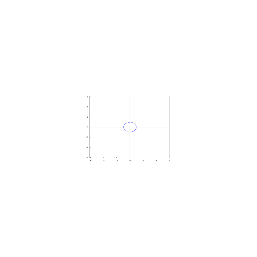
Figure 2: Example 1. The zeros (dark blue points) of the partial sum $S_{50}$ for the function $\widetilde{f}$ from Example 1. In complete accord with the classical Jentzsch–Szegő’s theorem (see [23], [51]), these zeros model the circle (the boundary of the convergence disc of the power series $\widetilde{f}_{0}\in\mathscr{H}(0)$).

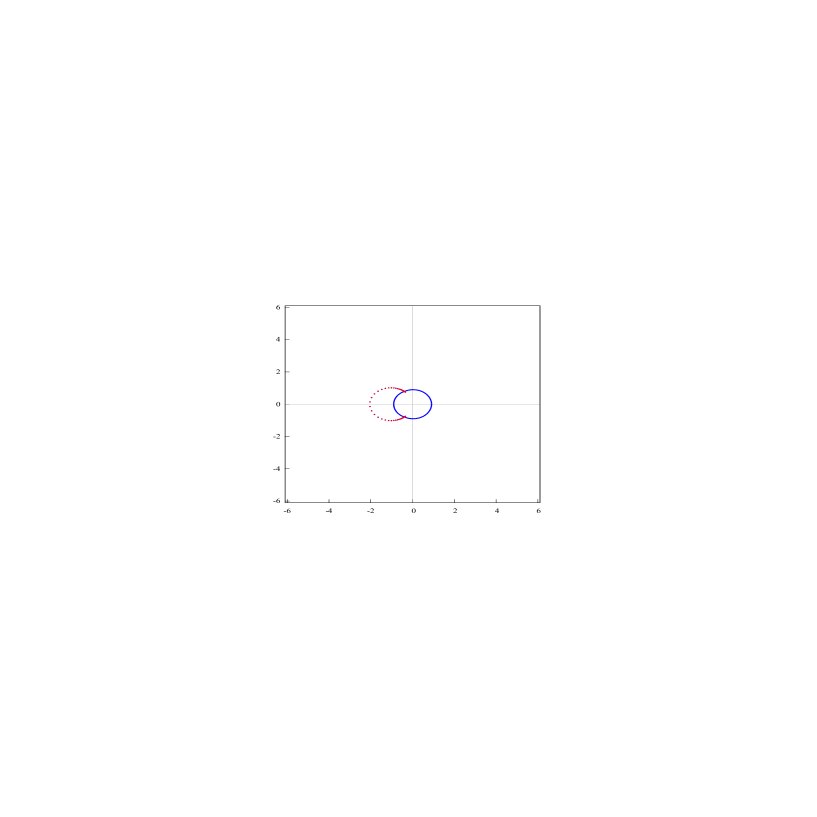
Figure 3: Example 1. The zeros of the partial sum $S_{100}$ (dark blue points) and the poles of the diagonal PA $[50/50]_{\widetilde{f}_{0}}$ (red points). It is clearly seen that from the zeros and poles of PA one can find the branch points of a multivalued analytic function, while this cannot be achieved using the zeros of the partial sums. The convergence radius of power series can be evaluated more accurately using the diagonal PA, rather than by employing the partial sums. The same number of Taylor coefficients of this series (101 coefficients $c_{0},c_{1},\dots,c_{100}$) were used to find the partial sum $S_{100}$ and the diagonal PA $[50/50]_{\widetilde{f}_{0}}$ .

So, an original function of the form (75) is defined by its series $\widetilde{f}_{0}$, which converges near the point $\zeta=0$, $\widetilde{f}_{0}\in\mathscr{H}(0)$. We are concerned with the problem of Weierstrass analytic continuation of the given power series $\widetilde{f}_{0}$ from the point $x=0$ along the real line to the point $x=6$ (it will be clear later that the choice of the point $x=6$ as an end-point of the extension is immaterial). Since the point $x=6$ is outside of the disc of convergence of the power series $\widetilde{f}_{0}$, the value $\widetilde{f}(6)$ cannot be (approximately) evaluated using partial sums of the series $\widetilde{f}_{0}$ of arbitrarily high order. Of course, this fact is a direct consequence of the Cauchy–Hadamard formula. However, there is another more transparent method to illustrate this fact in the framework of the approach discussed here. Namely, we analyze the limit distribution of free zeros and poles of rational approximants. Figure 2 depicts the numerically obtained distribution of the zeros of the partial sum $S_{50}$ of the series $\widetilde{f}_{0}$. It is transparent that the zeros of the partial sum $S_{50}$ model the circle (the boundary of the convergence disc of the power series $\widetilde{f}_{0}$). This is in full accord with the classical Jentzsch–Szegő theorem (see [23], [51]), according to which, along some subsequence depending on the function, the limit distribution of the zeros of partial sums exists and coincides with the Lebesgue measure of this circle. Looking ahead, we point out that Fig. 3 depicts the zeros of the partial sum $S_{100}$ and the zeros and poles of the diagonal PA $[50/50]_{\widetilde{f}_{0}}$ for the function from Example 1. It is transparent that using zeros and poles of the diagonal PA one can find the branch points of a multivalued analytic function, but this cannot be done using the zeros of partial sums. Even the radius of convergence of power series can be evaluated more accurately using the diagonal PA, rather than with the help of partial sums. It should be pointed out here that the same number of the coefficients of Taylor series was used to calculate the partial sum $S_{100}$ and the diagonal PA $[50/50]_{\widetilde{f}_{0}}$ (namely, 101 coefficients $c_{0},c_{1},\dots,c_{100}$ were used). Figure 2, which is formally unrelated to PA and Hermite–Padé polynomials, completely fits the general idea underlying the use of constructive rational approximants: the limit distribution of their free zeros and poles is most immediately related to the boundary of that domain in which these rational approximants realize an efficient analytic continuation of the original power series. Indeed, all poles of the partial sums of the power series are fixed at the infinity point. Hence the boundary of the convergence domain of partial sums is controlled by the limit distribution of free zeros of these partial sums.

To be more precise, let us clarify what is meant by a (singlevalued) analytic continuation of the power series $\widetilde{f}_{0}$ from the point $x=0$ to the right along the real line to the point $x=6$. Here we speak about the Weierstrass approach to the concept of an analytic function, which leads to the concept of a global analytic function. This approach resides on the concept of an analytic element (or simply an element) of an analytic function, which is defined as the convergent power series defined at a fixed point $\zeta_{0}$ and having the radius of convergence $R_{0}>0$. This will be briefly written as $\widetilde{f}_{0}\cong(\zeta_{0},\mathbb{D}(\zeta_{0},R_{0}))$, where $\mathbb{D}(\zeta_{0},R_{0}):=\{\zeta\in\mathbb{C}:|\zeta-\zeta_{0}|<R_{0}\}$. An element $\widetilde{f}_{1}\cong(\zeta_{1},\mathbb{D}(\zeta_{1},R_{1}))$ is called the direct analytic continuation of an $\widetilde{f}_{0}$ if $D:=\mathbb{D}(\zeta_{0},R_{0})\cap\mathbb{D}(\zeta_{1},R_{1})\neq\varnothing$ and $\widetilde{f}_{0}(\zeta)=\widetilde{f}_{1}(\zeta)$ for $\zeta\in D$. An element $\widetilde{f}_{N}=(\zeta_{N},\mathbb{D}(\zeta_{N},R_{N}))$ is called the analytic continuation of an element $\widetilde{f}_{0}$ along the path $\Gamma\subset\mathbb{C}$ (in particular, along the interval $[0,6]$) if there exists a chain of elements $\widetilde{f}_{j}=(\zeta_{j},\mathbb{D}(\zeta_{j},R_{j}))$, $j=1,\dots,N$, such that $\zeta_{j}\in\Gamma$ for all $j$ and each $\widetilde{f}_{j+1}$ is a direct analytic continuation of the element $\widetilde{f}_{j}$, $j=0,\dots,N-1$. Clearly, in our examples the Weierstrass extension from the point $x=0$ to the point $x=6$ along the positive real half-line is possible because all four branch points of the function $\widetilde{f}$ lie away from the real line $\mathbb{R}$.

5.2

We now proceed with numerically obtained Examples 1–3.

Example 1.

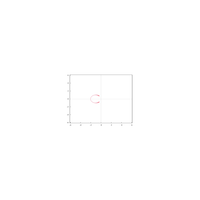
Figure 4: Example 1. The zeros and poles (dark blue and red points) of the diagonal PA $[50/50]_{\widetilde{f}_{0}}$, as constructed from the element $\widetilde{f}_{0}\in\mathscr{H}(0)$ from Example 1. In this case, the cut corresponding to the Stahl compact set lies entirely in the left half-plane. As a result, the value of the Weierstrass extension of the element $\widetilde{f}_{0}$ at the point $x=6$ can be approximately evaluated using the PA $[50/50]_{\widetilde{f}_{0}}(6)$.

In this example, the value of the parameter $a$ in representation (75) is negative, $a<0$. Correspondingly, both complex conjugate branch points $a\pm ib$ lie in the left half-plane. Figure 4 depicts the zeros and poles (dark blue and red points) of the PA $[50/50]_{\widetilde{f}_{0}}$, as constructed from an element $\widetilde{f}_{0}\in\mathscr{H}(0)$. In this case, the cut corresponding to the Stahl compact set lies entirely in the left half-plane. Thus, the values of the Weierstrass extension of the element $\widetilde{f}_{0}$ at the point $x=6$ can be approximately evaluated using the PA $[50/50]_{\widetilde{f}_{0}}(6)$. Increasing the order of the PA $[n/n]_{\widetilde{f}_{0}}$, we will increase the accuracy of calculation of the value $\widetilde{f}_{0}(6)$ in accordance with (8) and following well-known rules for evaluating PA.

Example 2.

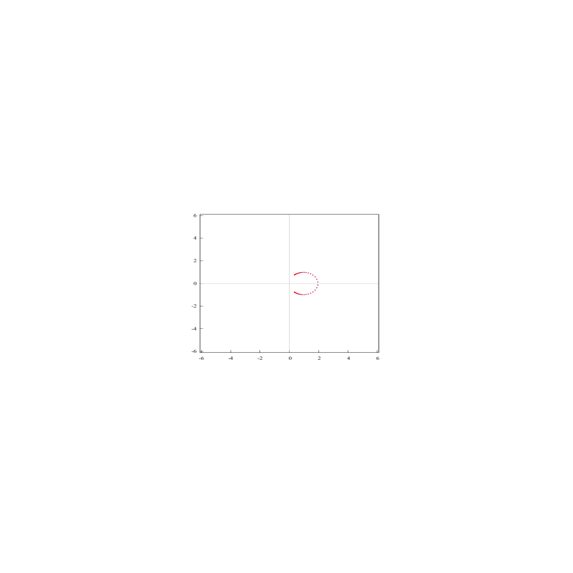
Figure 5: Example 2. The zeros and poles (dark blue and red points) of the diagonal PA $[50/50]_{\widetilde{f}_{0}}$, as constructed from the element $\widetilde{f}_{0}\in\mathscr{H}(0)$ from Example 2. In this case, the cut corresponding to the Stahl compact set intersects the real line between the points $x=0$ and $x=6$. Hence, the value of the multivalued function $\widetilde{f}$ at the point $x=6$, as calculated from the PA $[n/n]_{\widetilde{f}_{0}}$ as $n\to\infty$, is different from the value of the Weierstrass extension of the power series $\widetilde{f}_{0}$ from the point $x=0$ to the point $x=6$.

In this example we choose a positive $a$ in representation (75). Thus, the pair of branch points $a\pm ib$ of the element $\widetilde{f}_{0}$ now lies in the right half-plane. Evaluation of zeros and poles of the diagonal PA $[50/50]_{\widetilde{f}_{0}}$ of the germ $\widetilde{f}_{0}$ shows (see Fig. 5) that the cut corresponding to the Stahl compact set intersects the real line between the points $x=0$ and $x=6$. Therefore, the value of the multivalued function $f$ at the point $x=6$, as obtained from the PA $[n/n]_{\widetilde{f}_{0}}$ as $n\to\infty$, does not agree with the value of the Weierstrass extension of the power series $\widetilde{f}_{0}$ from the point $x=0$ to the point $x=6$.

Let us now employ the results of § 4.3. We employ in our setting relations (71) and (72) and the above results on the limit distribution of the zeros of Hermite–Padé polynomials. They will be used to study the topology of the Nuttall partition into sheets of that three-sheeted R.s. $\mathfrak{R}_{3}(w)$ which is associated to the germ $\widetilde{f}_{0}$ of the function (75) (such a surface is called a Nuttall surface). As was pointed out in § 4.3, relations (71) and (72) were obtained for a germ given at the point at infinity. For a germ defined at the point $\zeta=0$, all these results remain valid under the corresponding modification of the Nuttall partition into sheets to the case under consideration of a germ defined at the point $\zeta=0$.

Using this example, we shall show how the Hermite–Padé polynomials, as given by (69) and (70) and relations (71) and (72) can be used in the case when the diagonal PA are unfit for numerical realization of the procedure for Weierstrass extension of a given germ.

We cannot in fact study the structure of the boundaries $F^{(1,2)}$ and $F^{(2,3)}$ between three sheets of the R.s. $\mathfrak{R}_{3}(w)$ directly with the help of Hermite–Padé polynomials. However, based on (71) and (72) we can understand the structure of the projections $E_{2}=\pi_{3}(F^{(1,2)})$ and $F_{2}=\pi_{3}(F^{(2,3)})$ of these boundaries to the Riemann sphere, derive necessary information from this knowledge, and make appropriate conclusions on this basis.

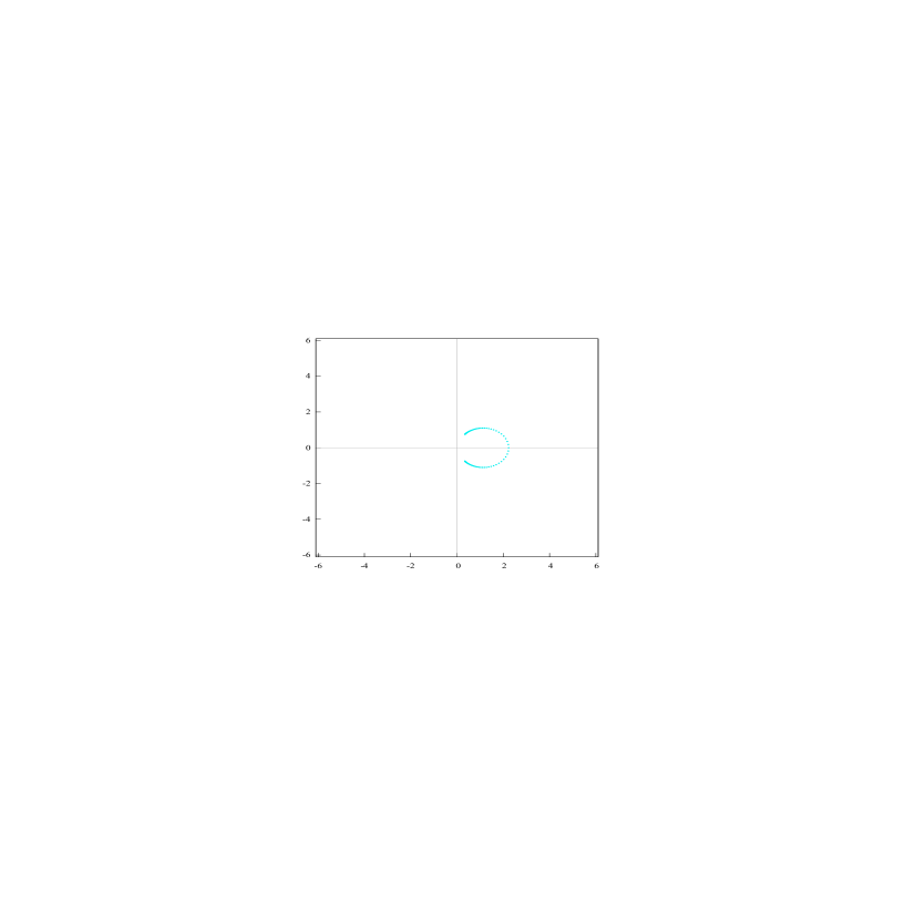
Figure 6: Example 2. The zeros (light blue points) of the type II Hermite–Padé polynomial $Q_{2n}$ for $n=50$. By (71), the corresponding cut is the compact set $E_{2}$ modeled by 100 zeros of this polynomial. This compact set $E_{2}$, as well as the Stahl compact set, intersects the real line between the points $x=0$ and $x=6$. Thus, from representation (71) one cannot find the sought-for value $\widetilde{f}_{0}(6)$ of the function. But from the above it follows that from (71) one can evaluate $\widetilde{f}_{0}(x^{(1)})$ at $x=6$ (we note once again that this value is distinct from the sought-for Weierstrass value $\widetilde{f}_{0}(6)$).

Figure 6 shows the zeros (light blue points) of the type II Hermite–Padé polynomial $Q_{2n}$ for $n=50$. By (71), the corresponding cut is the compact set $E_{2}$ modeled by 100 zeros of this polynomial. This compact set $E_{2}$, as well as the Stahl compact set, intersects the real line between the points $x=0$ and $x=6$. This being so, using (71) one cannot find the required value of the function $\widetilde{f}_{0}(6)$. At first sight, the situation is similar to that encountered in an attempt to employ the diagonal PA to find the value $\widetilde{f}_{0}(6)$. However this is not so. From the above it follows that with the help of (71) we can find the value $\widetilde{f}_{0}(x^{(1)})$ at $x=6$ (we note once again that this value does not agree with the sought-for Weierstrass value $\widetilde{f}_{0}(6)$).

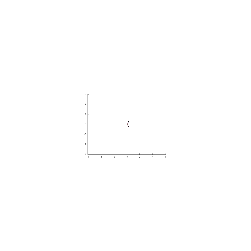
Figure 7: Example 2. The zeros (red, dark blue and black points) of the type I Hermite–Padé polynomial $Q_{\mathbf{n},j}$ for $\mathbf{n}=(50,50)$.

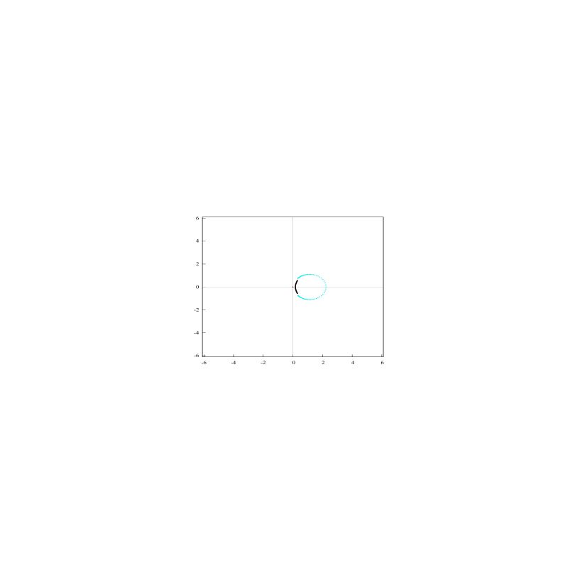
Figure 8: Example 2. The figure combines Figs. 6 and 7. It is seen that even though the compact set $F_{2}$, which attracts the zeros of the type I Hermite–Padé polynomials, intersects the real line between the points $x=0$ and $x=6$, it still lies to the left of the compact set $E_{2}$. It follows that the sought-for Weierstrass value $\widetilde{f}_{0}(6)$ agrees with the value $\widetilde{f}(x^{(2)})$ for $x=6$. Hence this value can be evaluated by successive applications of relations (71) and (72).

Let us now proceed to the type I Hermite–Padé polynomials $Q_{\mathbf{n},j}$ with $\mathbf{n}=(50,50)$. Their zeros (red, dark blue, and black points) are depicted in Fig. 7. Figure 8 combines Figs. 6 and 7. For the compact set $F_{2}$, which attracts the zeros of type I Hermite–Padé polynomials, Fig. 8 shows that even though this set intersects the real line between the points $x=0$ and $x=6$, but it still lies to the left of the compact set $E_{2}$. These compact sets $E_{2}$ and $F_{2}$, which are projections of the boundaries between the sheets of the Nuttall surface $\mathfrak{R}_{3}(w)$, reflect the following properties of the Nuttall partition of the R.s. $\mathfrak{R}_{3}(w)$ into sheets from the viewpoint of the Weierstrass extension of the original germ $\widetilde{f}_{0}$. When realizing the Weierstrass extension of the germ $\widetilde{f}_{0}$ from the point $x=0$ to the point $x=6$ along the positive real half-line, we will cross at some point $x=x_{1}\in(0,6)$ the compact set $E_{2}$. Thus, at this instant a transition from the first sheet $\mathfrak{R}^{(1)}_{3}$ of the R.s. $\mathfrak{R}_{3}(w)$ to the second sheet $\mathfrak{R}^{(2)}_{3}$ of this R.s. takes place. Further motion in accordance with the Weierstrass procedure to the point $x=6$ proceeds already along the second sheet $\mathfrak{R}^{(2)}_{3}$ of the R.s. $\mathfrak{R}_{3}(w)$. The compact set $F_{2}=\pi_{3}(F^{(2,3)})$ lies to the left of the compact set $E_{2}=\pi_{3}(F^{(1,2)})$. Hence, when moving further to the right along the second sheet $\mathfrak{R}^{(2)}_{3}$ to the point $x^{(2)}$, where $x=6$, we will always be only on the second sheet and will not cross the boundary $F^{(2,3)}$ between the second and third sheets of the R.s. $\mathfrak{R}_{3}(w)$. As a result, the sought-for Weierstrass extension $\widetilde{f}_{0}(6)$ coincides with the value $\widetilde{f}(x^{(2)})$ at $x=6$. Consequently, this value can be evaluated by a repeated application of relations (71) and (72).

Example 3.

Let us now proceed with the third example. In this example, the parameters $a$ and $b$ in representation (75) are the same as in Example 2. However, the parameter $A_{1}$ is now altered. As in Example 2, the Stahl compact set for the germ $\widetilde{f}_{0}$ is the same circular arc passing through the three points $\zeta=0,1/(a\pm ib)$. As before, this arc intersects the positive real half-line between the points $x=0$ and $x=6$.

Proceeding as in Example 2, let us find for the germ $\widetilde{f}_{0}$ the zeros of the type II Hermite–Padé polynomial $Q_{2n}$ for $n=50$ and the zeros of the type I Hermite–Padé polynomials $Q_{\mathbf{n},j}$, $j=0,1,2$, for $\mathbf{n}=(50,50)$. Using these data and employing relations (71) and (72), we analyze the structure of the Nuttall partition into sheets associated with the germ $\widetilde{f}_{0}$ of the three-sheeted R.s. $\mathfrak{R}_{3}(w)$. In accordance to (71), the zeros of the polynomial $Q_{2n}$ model the compact set $E_{2}=\pi_{3}(F^{(1,2)})$, while the zeros of the polynomials $Q_{\mathbf{n},j}$ model the compact set $F_{2}=\pi_{3}(F^{(2,3)})$. As in Example 2, both these compact sets intersect the positive real half-line between the points $x=0$ and $x=6$. But now, in contrast to Example 2, the compact set $F_{2}$ lies to the right of the compact set $E_{2}$ (see Fig. 10). For the problem under consideration this means the following. In the realization of the Weierstrass extension, when moving to the right of the point $x=0$ along the real line to the point $x=6$, we meet the compact set $E_{2}$ at some $x=x_{1}$, and hence, the subsequent realization of the Weierstrass extension will in fact proceed on the second sheet $\mathfrak{R}^{(2)}_{3}$ of the Nuttall surface $\mathfrak{R}_{3}(w)$. As the motion continues further to the right from the point $x=x_{1}$ to the point $x=6$, we intersect the compact set $F_{2}$ at some point $x=x_{2}$. This means that at this time we moved from the second sheet of the R.s. $\mathfrak{R}_{3}(w)$ to its third sheet $\mathfrak{R}^{(3)}_{3}$. Further realization of the Weierstrass procedure means that the actual motion now proceeds already along the third sheet $\mathfrak{R}^{(3)}_{3}$ of the R.s. $\mathfrak{R}_{3}(w)$. However, as was already pointed out above, the original germ $\widetilde{f}_{0}$ cannot be continued on this third sheet as a singlevalued analytic function, because for such a continuation appropriate cuts should be drawn on the third sheet. Due to this obstacle, which is inherent in the realization of the Weierstrass procedure by the compact set $F^{(2,3)}$ (the boundary between the second and third sheets of R.s. $\mathfrak{R}_{3}(w)$), we cannot find the required value of $\widetilde{f}_{0}(6)$ using the Hermite–Padé polynomials $Q_{2n}$ and $Q_{\mathbf{n},j}$ for $\mathbf{n}=(n,n)$ in the way we did it in Example 2, because on the third sheet $\mathfrak{R}^{(3)}_{3}$ of the R.s. $\mathfrak{R}_{3}(w)$ relations (71) and (72) do not apply anymore.

Clearly, in this situation to realize the Weierstrass extension one needs to augment the family of germs $[1,\widetilde{f}_{0},\widetilde{f}_{0}^{2}]$ with the germ $\widetilde{f}_{0}^{3}$, increase the dimension of multiindices by 1, and proceed with constructions (9)–(11), (18) and (24) corresponding to the multiindices $\mathbf{n}=(n,n,n)$, $\mathbf{n}_{1}=(n,n-1,n-1)$, $\mathbf{n}_{2}=(n,n,n-1)$ and $\mathbf{n}_{3}=(n,n,n)$. As a result, on the four-sheeted R.s. $\mathfrak{R}_{4}(\widetilde{f})$ there appears the Nuttall partition into sheets corresponding to the point $\zeta=0$ at which the original germ $\widetilde{f}_{0}$ is given. The results of the corresponding numerical calculations with $n=50$ are shown in Fig. 10–13 (the zeros and poles of the diagonal PA $[50/50]_{\widetilde{f}_{0}}$ are located quite similarly to Example 2, and hence are not shown here).

Figure 11 depicts the zeros of the type II Hermite–Padé polynomial $Q_{3n}$ for $n=50$ (yellow points), which model in accordance with Theorem 5 the compact set $E=\pi_{4}(\Gamma^{(1,2)})$, where $\Gamma^{(1,2)}$ is the boundary between the first and second sheets of the R.s. $\mathfrak{R}_{4}(\widetilde{f})$. Besides, Figure 11 shows (light blue points) the zeros of the polynomial $S_{2n,1}$ for $n=50$, modeling the compact set $F=\pi_{4}(\Gamma^{(2,3)})$, where $\Gamma^{(2,3)}$ is the boundary between the second and third sheets of the R.s. $\mathfrak{R}_{4}(\widetilde{f})$. Figure 12 depicts (black points) the zeros of the polynomial $Q_{\mathbf{n},3}$, $\mathbf{n}=(n,n,n)$, for $n=50$, which model the compact set $E^{\prime}=\pi_{4}(\Gamma^{(3,4)})$, where $\Gamma^{(3,4)}$ is the boundary between the third and fourth sheets of the R.s. $\mathfrak{R}_{4}(\widetilde{f})$. Figure 13 combines Figs. 11 and 12. In this case, the realization of the Weierstrass extension from the point $x=0$ to the point $x=6$ along the positive real half-line means in fact the following. Moving to the right from the point $x=0$ to the point $x=6$ we meet the compact set $E$ at some point $x=x_{1}$. This means that when realizing the Weierstrass extension our further motion proceeds now along the second sheet $\mathfrak{R}^{(2)}_{4}$ of the R.s. $\mathfrak{R}_{4}(\widetilde{f})$. This continues until at some point $x=x_{2}$ we intersect the compact set $F$, which is the projection of the boundary $\Gamma^{(2,3)}$ between the second and third sheets of the R.s. $\mathfrak{R}_{4}(\widetilde{f})$. From this point on, our motion to the right takes place already along the third sheet $\mathfrak{R}^{(3)}_{4}$ of the R.s. $\mathfrak{R}_{4}(\widetilde{f})$. The fact that the compact set $E^{\prime}$, which is the projection of the boundary between the third and fourth sheets of the R.s. $\mathfrak{R}_{4}(\widetilde{f})$, lies to the left of the compact set $F$ (see Fig. 13, which combines Figs. 11 and 12), means for us that when moving to the right along the third sheet $\mathfrak{R}^{(3)}_{4}$ of the R.s. $\mathfrak{R}_{4}(\widetilde{f})$ we shall not meet the boundary between the third and fourth $\mathfrak{R}^{(4)}_{4}$ sheets of the R.s. $\mathfrak{R}_{4}(\widetilde{f})$. So, during the remaining time (until the point $x=6$ is reached) we shall in fact move along the third sheet. Note that the compact set $E^{\prime}$, as well as the compact sets $E$ and $F$, intersects the real line between the points $x=0$ and $x=6$ and lies to the left of the compact set $E$. This, however, has no effect on the implementation of the Weierstrass procedure, because the compact set $E^{\prime}$ is the projection of the boundary $\Gamma^{(3,4)}$ between the third and fourth sheets, which ‘‘is not seen’’ on the first and second sheets of the R.s. $\mathfrak{R}_{4}(\widetilde{f})$.

Thus, according to what has been said, the required Weierstrass value $\widetilde{f}_{0}(6)$ coincides with the value $\widetilde{f}(x^{(3)})$ of the function at $x=6$. According to the above Theorems 4–6, the required value of $\widetilde{f}_{0}(6)$ is evaluated by successive application of relations (60), (56) and  (50) (see also (61)–(63)).

Remark 8.

To conclude we note that the new method proposed here of efficient continuation of a power series beyond its disc of convergence guarantees the possibility, in the class of multivalued analytic functions with finite number of branch points, to realize the Weierstrass procedure arbitrarily far beyond the disc of convergence. To this end one needs to appropriately increase the dimensions of the employed multiindices.

By now there are practically no theoretical results justifying the use of the method of analytic continuation proposed here. We plan to offer the proofs of the above Theorems 1–3 and Theorems 4–6 in the separate papers [49] and [50], respectively. We propose to carry out numerical analysis of applied problems on the basis of the method proposed in the present paper.

It is worth pointing out that the new approach to the solution of the problem of efficient analytic continuation of power series was inspired not only by theoretical results and conjectures mentioned above, but also by the numerical experiments, whose results are given in the papers [20], [21] and [22].

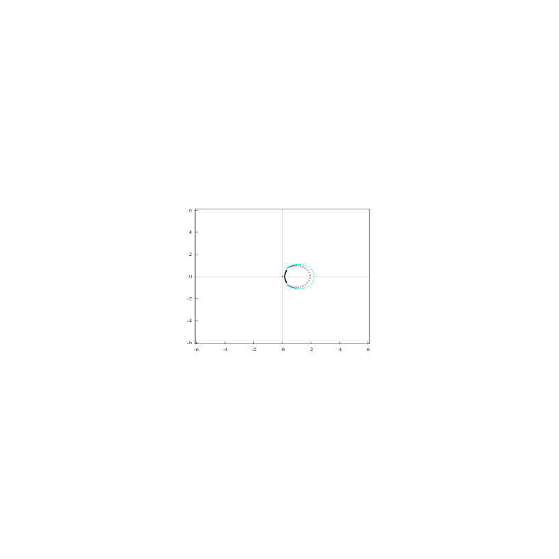
Figure 9: Example 2. The zeros and poles (dark blue and red points) of the PA $[50/50]_{\widetilde{f}_{0}}$, as constructed from the element $\widetilde{f}_{0}\in\mathscr{H}(0)$ from Example 2. The figure also shows the zeros (light blue points) of the type II Hermite–Padé polynomial $Q_{2n}$ for $n=50$ and the zeros (red, dark blue and black points) of the type I Hermite–Padé polynomials $Q_{\mathbf{n},j}$ for $\mathbf{n}=(50,50)$. It is seen that all three compact sets $S$, $E_{2}$, and $F_{2}$ are distinct from each other.

Figure 11: Example 3. The zeros (yellow points) of the type II Hermite–Padé polynomial $Q_{3n}$ for $n=50$, which model in accordance with Theorem 5 the compact set $E=\pi_{4}(\Gamma^{(1,2)})$. Moreover, the figure depicts the zeros (light blue points) of the polynomials $S_{2n,1}$ for $n=50$, which model the compact set $F=\pi_{4}(\Gamma^{(2,3)})$.

Figure 12: Example 3. The zeros (black points) of the polynomial $Q_{\mathbf{n},2}$, $\mathbf{n}=(n,n,n)$, for $n=50$, which model the compact set $E^{\prime}=\pi_{4}(\Gamma^{(3,4)})$.

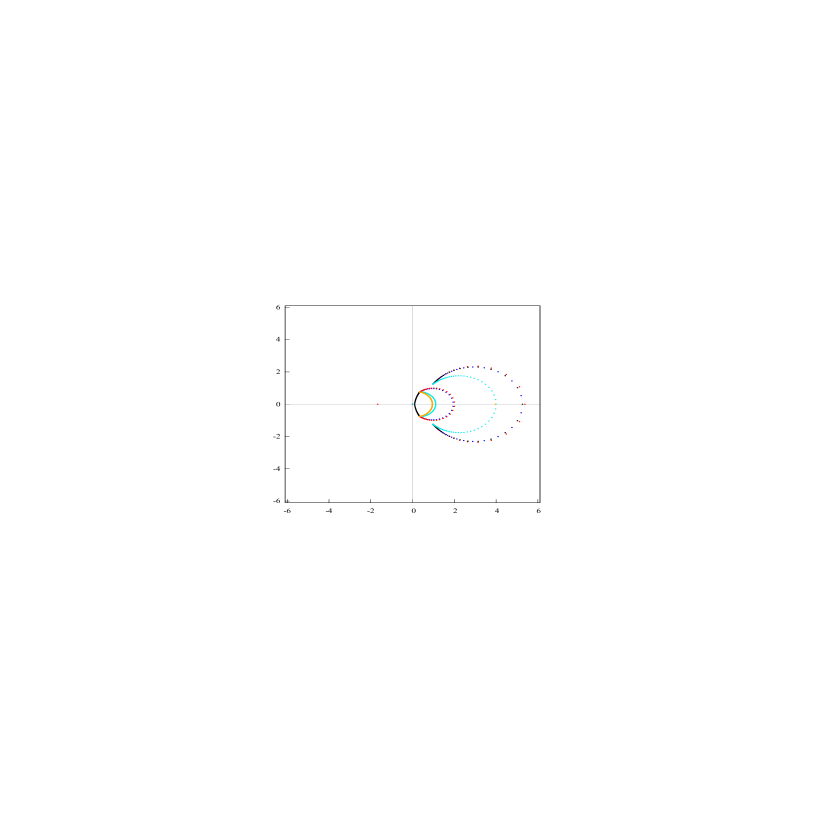
Figure 14: Example 3. The zeros and poles (dark blue and red points) PA $[50/50]_{\widetilde{f}_{0}}$, as constructed from the element $\widetilde{f}_{0}\in\mathscr{H}(0)$ from Example 3. Moreover, the figure depicts the zeros (light blue points) of the type II Hermite–Padé polynomial $Q_{2n}$ for $n=50$ and the zeros (red, dark blue and black points) of the type I Hermite–Padé polynomials $Q_{\mathbf{n},j}$ for $\mathbf{n}=(50,50)$ (Fig. 10). Besides, it shows the zeros (yellow points) of the type II Hermite–Padé polynomial $Q_{3n}$, the zeros (yellow points) of the polynomial $S_{2n,1}$, and the zeros (black points) of the type I Hermite–Padé polynomial $Q_{\mathbf{n},2}$ for $\mathbf{n}=(n,n,n)$, where $n=50$. It is clear that all six compact sets $S$, $E_{2},F_{2}$, $E,F$ and $E^{\prime}$ are distinct from each other.

References

- [1] A. I. Aptekarev, Strong asymptotics of multiply orthogonal polynomials for Nikishin systems, Sb. Math., 1999, vol 190, no 5, pp. 631–669
- [2] A. I. Aptekarev, Asymptotics of Hermite–Pade approximants for a pair of functions with branch points, Dokl. Math. vol 78, 2008, no 2, pp. 717–719
- [3] A. I. Aptekarev, V. G. Lysov, Systems of Markov functions generated by graphs and the asymptotics of their Hermite-Padé approximants, Sb. Math., 2010, vol 201, no 2, pp. 183–234
- [4] A. I. Aptekarev, V. I. Buslaev, A. Martínez-Finkelshtein, S. P. Suetin, Padé approximants, continued fractions, and orthogonal polynomials, Uspekhi Mat. Nauk, 2011, vol 66, no 6(402), pp. 37–122
- [5] Alexander I. Aptekarev, Maxim L. Yattselev, Padé approximants for functions with branch points – strong asymptotics of Nuttall–Stahl polynomials, Acta Mathematica, vol 215, no 2, pp. 217–280 , 2015
- [6] A. I. Aptekarev, A. I. Bogolyubskii, M. Yattselev, Convergence of ray sequences of Frobenius-Padé approximants, Sb. Math., 2017, vol 208, no 3, pp. 313–334
- [7] N. U. Arakelian, On efficient analytic continuation of power series, Mat. Sb. (N.S.), 1984, vol 124(166), no 1(5), pp. 24–44 transl: Math. USSR-Sb., 1985, vol 52, no 1, pp. 21–39
- [8] Norair Arakelian, Wolfgang Luh, Efficient analytic continuation of power series by matrix summation methods, Comput. Methods Funct. Theory, vol. 2, 2002, no 1, pp. 137–153
- [9] N. U. Arakelyan, Efficient analytic continuation of power series and the localization of their singularities (in Russian), Izv. Nats. Akad. Nauk Armenii Mat. , vol. 38, 2003, no 4 , pp. 5–24 transl: in J. Contemp. Math. Anal., vol. 38, no 4, pp. 2–20, 2004
- [10] L. Bieberbach, Analytische Fortsetzung, Berlin–Göttingen–Heidelberg, Springer-Verlag, 1955, ii+168
- [11] E. Borel, Lecons sur les fonctions de variables reelles et les developpements en series de polynomes, Gauthier-Villars, Paris, 1905
- [12] D. Barrios Rolanía, J. S. Geronimo, G. López Lagomasino, High-order recurrence relations, Hermite-Padé approximation and Nikishin systems, Sb. Math., 2018, vol. 209, no 3, pp. 385–420
- [13] V. I. Buslaev, S. P. Suetin, On Equilibrium Problems Related to the Distribution of Zeros of the Hermite–Padé Polynomials, in book: Modern problems of mathematics, mechanics, and mathematical physics, Collected papers, Proc. Steklov Inst. Math., 2015, vol. 290, pp. 256–263
- [14] E. M. Chirka, Riemann surfaces, Lekts. Kursy NOC, 2006, vol. 1, Steklov Math. Institute of RAS, Moscow, 106 pp.
- [15] U. Fidalgo Prieto, A. Lopez Garcia, G. Lopez Lagomasino, V. N. Sorokin, Mixed type multiple orthogonal polynomials for two Nikishin systems, Constructive Approximation , 2010, vol. 32, pp. 255–306
- [16] U. Fidalgo Prieto, G. Lopez Lagomasino, Nikishin Systems Are Perfect Constr. Approx., vol. 34, no 3 , 2011, pp. 297–356
- [17] A. A. Gonchar, E. A. Rakhmanov, On the convergence of simultaneous Padé approximants for systems of functions of Markov type, Proc. Steklov Inst. Math., 1983, vol. 157, pp. 31–50
- [18] A. A. Gonchar, E. A. Rakhmanov, Equilibrium measure and the distribution of zeros of extremal polynomials Math. USSR-Sb., 1986, vol. 53, no 1, pp. 119–130
- [19] A. A. Gonchar, E. A. Rakhmanov, V. N. Sorokin, Hermite–Pade approximants for systems of Markov-type functions Sb. Math., 1997, vol. 188, no 5, pp. 671–696
- [20] N. R. Ikonomov, R. K. Kovacheva, S. P. Suetin, 2015, Some numerical results on the behavior of zeros of polynomials, 95 pp., arXiv: 1501.07090
- [21] N. R. Ikonomov, R. K. Kovacheva, S. P. Suetin, 2015, On the limit zero distribution of type I Hermite-Padé polynomials, 67 pp., arXiv: 1506.08031
- [22] Nikolay R. Ikonomov, Ralitza K. Kovacheva, Sergey P. Suetin, 2016, Zero Distribution of Hermite–Padé Polynomials and Convergence Properties of Hermite Approximants for Multivalued Analytic Functions, 37 pp. arXiv: 1603.03314
- [23] R. Jentzsch, Untersuchungen zur Theorie der Folgen analytischer Funktionen, Acta Math., vol. 41, no 1 , 1916, pp. 219–251
- [24] A. V. Komlov, N. G. Kruzhilin, R. V. Palvelev, S. P. Suetin, Convergence of Shafer quadratic approximants, Russian Math. Surveys, 2016, vol. 71, no 2, pp. 373–375
- [25] A. V. Komlov, R. V. Palvelev, S. P. Suetin, E. M. Chirka, Hermite–Padé approximants for meromorphic functions on a compact Riemann surface, Russian Math. Surveys, 2017, vol. 72, no 4, pp. 671–706
- [26] Guillermo Lopez Lagomasino, Walter Van Assche, Riemann–Hilbert analysis for a Nikishin system, Sb. Math., 2018, vol. 209, no 7 arXiv: 1612.07108
- [27] A. Lopez-Garcia, E. Mina-Diaz, Nikishin systems on star-like sets: algebraic properties and weak asymptotics of the associated multiple orthogonal polynomials, Sb. Math., 2018, vol. 209, no 7
- [28] A. I. Markushevich, Theory of functions of a complex variable, vol. II, Revised English edition translated and edited by Richard A. Silverman, Prentice-Hall, Inc. Englewood Cliffs, N.J., 1965, xii+333 pp.
- [29] Andrei Martínez-Finkelshtein, Evguenii A. Rakhmanov, Sergey P. Suetin, Asymptotics of type I Hermite–Padè polynomials for semiclassical functions, in book: Modern trends in constructive function theory, Contemp. Math., 2016, vol. 661, pp. 199–228; arxiv: 1502.01202
- [30] E. M. Nikishin, Asymptotic behavior of linear forms for simultaneous Padé approximants, Soviet Math. (Iz. VUZ), 1986, vol. 30, no 2, pp. 43–52
- [31] Nikishin, E. M.; Sorokin, V. N., Rational approximations and orthogonality, Translated from the Russian by Ralph P. Boas, Translations of Mathematical Monographs, vol. 92, American Mathematical Society, Providence, RI, 1991, viii+221 , pp. ISBN: 0-8218-4545-4
- [32] J. Nuttall, R. S. Singh, Orthogonal polynomials and Padé approximants associated with a system of arcs, 1977, J. Approx. Theory, vol. 21, pp. 1–42
- [33] J. Nuttall, Asymptotics of diagonal Hermite–Pade polynomials, 1984, J. Approx.Theory , vol. 42 , pp. 299–386
- [34] P. Painlevé, Note I., Sur le développement des fonctions analytiques, pp. 101–148 in book: E. Borel, Lecons sur les fonctions de variables reelles et les developpements en series de polynomes, Gauthier-Villars, Paris, 1905
- [35] E. A. Rakhmanov, S. P. Suetin, The distribution of the zeros of the Hermite-Padé polynomials for a pair of functions forming a Nikishin system, Sb. Math., 2013, vol. 204, no 9, pp. 1347–1390
- [36] E. A. Rakhmanov, The Gonchar-Stahl -theorem and associated directions in the theory of rational approximations of analytic functions, Sb. Math., 2016, vol. 207, no 9, pp. 1236–1266
- [37] E. A. Rakhmanov, Zero distribution for Angelesco Hermite–Padé polynomials Uspekhi Mat. Nauk, 2018, vol. 73, no 3(441), pp. 89–156
- [38] Menahem Schiffer, Donald C. Spencer, Functionals of finite Riemann surfaces, Princeton University Press, Princeton, N. J., 1954, x+451 pp.
- [39] R. E. Shafer, On Quadratic Approximation, SIAM Journal on Numerical Analysis, 1974, vol. 11, no 2, pp. 447–460
- [40] V. N. Sorokin, Simultaneous approximation of several linear forms (Russian), Vestnik Moskov. Univ. Ser. I Mat. Mekh., 1983, no 1, pp. 44–47
- [41] H. Stahl, Asymptotics of Hermite–Padé polynomials and related convergence results. A summary of results, in book: Nonlinear numerical methods and rational approximation Wilrijk, 1987, pp. 23–53, Math. Appl., vol. 43, Reidel Dordrecht, 1988
- [42] H. Stahl, The convergence of Padé approximants to functions with branch points, J. Approx. Theory, vol. 91, 1997, no 2, pp. 139–204
- [43] Herbert R. Stahl, Sets of Minimal Capacity and Extremal Domains, 112 pp., arXiv: 1205.3811
- [44] S. P. Suetin, Distribution of the zeros of Padé polynomials and analytic continuation, Russian Math. Surveys, 2015, vol. 70, no 5, pp. 901–951
- [45] S. P. Suetin, An Analog of Pólya’s Theorem for Multivalued Analytic Functions with Finitely Many Branch Points, Math. Notes, 2017, vol. 101, no 5, pp. 888–898
- [46] S. P. Suetin, On the distribution of the zeros of the Hermite–Padé polynomials for a quadruple of functions, Russian Math. Surveys, 2017, vol. 72, no 2, pp. 375–377
- [47] S. P. Suetin, Distribution of the zeros of Hermite–Padé polynomials for a complex Nikishin system, Russ. Math. Serv., 2018, vol. 73, no 2(440), pp. 183–184
- [48] S. P. Suetin, On a new approach to the problem of the zero distribution of Hermite–Padé polynomials for a Nikishin system, Proc. Inst. Steklov, 2018, vol. 301; arXiv: 1805.07577
- [49] S. P. Suetin, Hermite–Padé polynomials and analytic continuation: the real case, In preparation, 2018
- [50] S. P. Suetin, Hermite–Padé polynomials and analytic continuation: the complex case, In preparation, 2018
- [51] G. Szegő, Uber die Nullstellen von Polynomen, die in einem Kreise gleichmassig konvergieren, Sitzungsber. Berl. Math. Ges., vol. 21, 1922, pp. 59–64