Level Crossing in Random Matrices. II. Random perturbation of a random matrix

Abstract.

In this paper we study the distribution of level crossings for the spectra of linear families $A+\lambda B,$ where $A$ and $B$ are square matrices independently chosen from some given Gaussian ensemble and $\lambda$ is a complex-valued parameter. We formulate a number of theoretical and numerical results for the classical Gaussian ensembles and some generalisations. Besides, we present intriguing numerical information about the distribution of monodromy in case of linear families for the classical Gaussian ensembles of $3\times 3$ matrices.

1. Introduction

Given a linear operator family

$$C=A+\lambda B,$$ (1.1)

analysis of the dependence of its spectrum on a perturbative parameter $\lambda$ is a typical problem both in fundamental natural sciences and applications, see e.g. the classical treatise [Ka]. Depending on the situation $\lambda$ is considered as a real or a complex-valued parameter.

Level crossings of the spectrum (i.e., collisions of the eigenvalues) in the family (1.1) unavoidably occur upon the analytic continuation of a real perturbation parameter $\lambda$ into the complex plane, where an intricate pattern of permutations of the eigenvalues arises due to monodromy of the spectrum at each of the level crossing points. The positions of level crossings and monodromy of the spectrum at each of them constitute an important piece of information about the spectral properties of the linear family (1.1) and the analytic structure of its spectral surface. Level crossings determine, in particular, the accuracy of perturbative series in $\lambda$.

Since the late 60s, motivated by a number of fascinating observations by C. M. Bender and T. T. Wu [BW], physicists and mathematicians started considering various cases where $A$ and $B$ are, for example, self-adjoint while $\lambda$ is complex-valued. A very small sample of such studies can be found in e.g., [MNOP, Ro, CHM, SH, BDCP, Sm] and references therein.

Unfortunately, for a somewhat interesting concrete linear family (1.1), it is usually quite difficult to exactly describe the positions of level crossings and especially the monodromy of the spectrum, when $\lambda$ encircles closed curves avoiding them. As an illustration of specific examples of the physics origin, the reader might consult [ShTaQu] and [ShT], where the cases of the quasi-exactly solvable quartic and sextic are considered. The corresponding locations of level crossings are shown in Figure 1 below. Although in both cases numerical experiments reveal very clear and intriguing patterns for the location of level crossings as well as the corresponding monodromy, mathematical proofs explaining these lattice-type patterns in Figure 1 are unavailable at present.

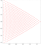
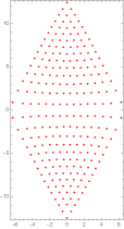
Figure 1. Level crossings for the quasi-exactly solvable quartic (left) and sextic (right), see [ShTaQu] and [ShT].

Taking this circumstance into account, in [ShZa1] we considered the problem of finding the distribution of level crossings within the framework of the random matrix theory and studied the case when $A$ is a fixed matrix while $B$ is a matrix distributed according to one of the standard Gaussian ensembles. (To the best of our knowledge, for the first time similar approach has been used in [ZVW]. For general information on the random matrix theory see e.g. [AGZ].)

The present paper being a sequel of [ShZa1], discusses level crossings in linear matrix families of the form (1.1), where both $A$ and $B$ are independent and equally distributed matrices belonging to a certain class of complex, real, real orthogonal or unitary Gaussian ensembles. To stress the equal rôle of matrices in (1.1), we denote them here by $A$ and $B$ as opposed to $V_{0}$ and $H$ in [ShZa1]. (A somewhat similar situation, when one randomly samples coefficients of a bivariate polynomial instead of the entries of a matrix has been earlier considered in [GP].)

We start with complex Gaussian ensembles. Recall that the complex (non-symmetric) Gaussian ensemble $GE_{n}^{{\mathbb{C}}}$ is the distribution on the space $Mat_{n}^{{\mathbb{C}}}$ of all complex-valued $n\times n$-matrices, where each entry of a random $n\times n$-matrix is an independent complex Gaussian variable distributed as $N(0,\frac{1}{2})+iN(0,\frac{1}{2})$.

Our first result is as follows.

Theorem 1.

For any positive integer $n$, if the matrices $A$ and $B$ are independently chosen from $GE_{n}^{{\mathbb{C}}},$ then the distribution of level crossings in (1.1) with respect to the affine coordinate $\lambda=x+iy$ of $\mathbb{C}$ is given by

$$\mathcal{P}_{{GE}_{n}^{{\mathbb{C}}}}(\lambda):=\mathcal{P}_{{GE}_{n}^{{\mathbb{C}}}}(x,y)dxdy=\frac{dxdy}{\pi(1+x^{{2}}+y^{{2}})^{{2}}}=\frac{dxdy}{\pi(1+|\lambda|^{{2}})^{{2}}}.$$ (1.2)

Remark 1.

In polar coordinates $(r,\theta)$ in the complex plane of parameter $\lambda$, the above distribution $\mathcal{P}_{{GE}_{n}^{{\mathbb{C}}}}(\lambda)$ has the form

$$\mathcal{P}_{{GE}_{n}^{{\mathbb{C}}}}(r,\theta)drd\psi=\frac{rdrd\theta}{\pi(1+r^{{2}})^{{2}}},$$

giving the radial CDF of the form

$$\Psi_{{GE}_{n}^{{\mathbb{C}}}}(r)=\frac{r^{{2}}}{1+r^{{2}}}.$$

Remark 2.

Let us realize $\mathbb{CP}^{{1}}\simeq S^{{2}}$ as the unit sphere in $\mathbb{R}^{{3}}$ with coordinates $(X,Y,Z)$ and identify the complex plane of parameter $\lambda=x+iy$ with the horizontal coordinate $(X,Y)$-plane, where $X$ corresponds to the real axis and $Y$ corresponds to the imaginary axis in $\mathbb{C}$. If we use the standard stereographic projection of the unit sphere in $\mathbb{R}^{{3}}$ from its north pole, i.e., from the point $(0,0,1)$ onto the $(X,Y)$-plane, then the usual area element of the sphere induced from the standard Euclidean structure in $\mathbb{R}^{{3}}$ is given by

$$dA=\frac{4dxdy}{(1+x^{{2}}+y^{{2}})^{{2}}}=\frac{4dxdy}{(1+|\lambda|^{{2}})^{{2}}}.$$

The latter fact implies that the r.h.s. of (1.2) presents the constant density $\frac{1}{4\pi}$ with respect to the standard Euclidean area measure on $S^{{2}}\simeq\mathbb{C}P^{{1}}$ compactifying the complex plane of parameter $\lambda$. (The constant density $\frac{1}{4\pi}$ provides the unit sphere with the total mass $1$.)

Remark 3.

Observe that formula (1.2) is independent of the size of $A$ and $B$ (and also of the variance of the matrix ensemble, if we allow to change it). For $n=1$, formula (1.2) gives the distribution of the quotient of two independent complex Gaussian random variables.

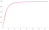
Figure 2. Radial density of level crossings for $A+\lambda B,$ where $A$ and $B$ are independently sampled from $GE_{6}^{{\mathbb{C}}}$; (we used 100 random pairs). The above diagram shows a perfect match of the numerical distribution of the absolute values of level crossings obtained in our sampling with the theoretical radial CDF $\frac{r^{{2}}}{1+r^{{2}}}$.

A number of further generalizations of Theorem 1 can be found in § 2.

Next we consider Gaussian orthogonal, Gaussian unitary, and real Gaussian ensembles. Recall that

(i) the Gaussian orthogonal ensemble $GOE_{n}^{{\mathbb{R}}}$ is the distribution on the space $Sym_{n}^{{\mathbb{R}}}$ of real-valued symmetric matrices, where each entry $e_{i,j}=e_{j,i},\;i<j$ of a matrix is an independent random variable distributed as $N(0,1)$, and each diagonal entry $e_{i,i}$ is independently distributed as $\sqrt{2}N(0,1)$;

(ii) the Gaussian unitary ensemble $GUE_{n}$-ensemble is the distribution on the space $\mathcal{H}_{n}$ of all Hermitian $n\times n$-matrices, where each entry $e_{i,j}=e_{j,i},\;i<j$ of a matrix is an independent random variable distributed as $N(0,\frac{1}{2})+iN(0,\frac{1}{2})$, and each diagonal entry $e_{i,i}$ is independently distributed as $N(0,1)$;

(iii) the real (non-symmetric) Gaussian ensemble $GE_{n}^{{\mathbb{R}}}$ is the distribution on the space $Mat_{n}^{{\mathbb{R}}}$ of real-valued $n\times n$ matrices, where each entry of a matrix is an independent real random variable distributed as $N(0,1)$.

In the case of $GOE_{n}^{{\mathbb{R}}}$ we have a theoretical result for $n=2$ and a conjecture for $n\geq 3$ based on computer simulations.

Theorem 2.

If the matrices $A$ and $B$ are independently chosen from $GOE_{2}^{{\mathbb{R}}}$, then the distribution of level crossings in (1.1) is uniform on $\mathbb{CP}^{{1}}\supset\mathbb{C},$ i.e., their density is given by the right-hand side of (1.2).

Remark 4.

One can easily check that the distribution of level crossings for $A$ and $B$ independently taken from $GOE_{1}^{{\mathbb{R}}}$ is uniform on the real projective line $\mathbb{R}P^{{1}}$.

Extensive numerical experiments strongly support the following guess illustrated in Fig. 3.

Conjecture 1.

For any fixed size $n>2$, if the matrices $A$ and $B$ are independently chosen from $GOE_{n}^{{\mathbb{R}}}$, then the distribution of level crossings in (1.1) is uniform on $\mathbb{CP}^{{1}}\supset\mathbb{C}.$

Remark 5.

Notice that on Fig. 3 one can hardly see the difference between the statistical results for $n=2,4,6,8,10$ and the theoretical CDFs of the uniform distribution on $\mathbb{CP}^{{1}}$. Although the simple (conjectural) answer for level crossing distribution in the $GOE$-case presented in Theorem 2 and Conjecture 1 indicates the possible existence of some extra symmetry complementing the $SO_{2}$-action presented in § 3, we were not able to find such.

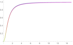
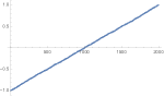
Figure 3. Numerical and theoretical radial and angle CDFs for (1.1) for $n=2,4,6,8,10$ with $A$ and $B$ taken from $GOE_{n}$ are practically indistinguishable.

Our next results deal with Gaussian unitary ensembles. Here again we have a theoretical result for $n=2$ and numerical plots for higher $n$.

Theorem 3.

If the matrices $A$ and $B$ are independently chosen from $GUE_{2},$ then the distribution of level crossings in $\mathbb{C}$ is given by

$$\mathcal{P}_{GUE_{2}}(x,y)dxdy=\frac{4|y|dxdy}{\pi(1+x^{{2}}+y^{{2}})^{{3}}}=\frac{1}{\pi}\left|\frac{y}{1+x^{{2}}+y^{{2}}}\right|\frac{4dxdy}{(1+x^{{2}}+y^{{2}})^{{2}}},$$ (1.3)

which matches the general formula (3.1).

In the cylindrical coordinates $(\psi,Y)$ on $\mathbb{C}P^{{1}}$, where $0\leq\psi\leq 2\pi$ and $-1\leq Y\leq 1$, one has

$$\mathcal{P}_{GUE_{2}}(\psi,Y)d\psi dY=\frac{|Y|d\psi dY}{2\pi}.$$ (1.4)

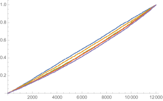
Figure 4. Empirical distributions of $|Y|$ for (1.1) taken from $GUE_{n}$ with $n=2,3,4,5,6$. (Curves corresponding to the increasing values of $n$ lie one below the other; the blue straight line corresponds to $n=2$, see (1.4).)

At present, we do not have explicit (even conjectural) formulas for the densities $\mathcal{P}_{{GUE}_{n}}(x,y)$, for $n\geq 3$ similar to (1.4). But we carried out substantial numerical experiments for matrix sizes up to $6$ conducted as follows. For each $n\in\{2,...,6\},$ sampling independently pairs of $GUE_{n}$-matrices, we calculated 12,000 level crossing points for every $n$ and plotted the values of $|Y|$ for obtained level crossings in increasing order, see Fig. 4. These numerical experiments strongly suggest the following.

Conjecture 2.

There exists a limiting distribution $\mathcal{P}_{GUE_{\infty}}(Y):=\lim_{n\to\infty}\mathcal{P}_{GUE_{n}}(Y)$.

Our final results deal with the case when $A$ and $B$ are independently taken from the $GE_{n}^{{\mathbb{R}}}$-ensemble. Theoretical results are available for $n=2$ as well as an explicit general conjecture about the asymptotics of level crossings when $n\to\infty$. The next statement describes the distribution of the coefficients of the random real quadratic discriminantal polynomial whose roots are the two level crossing points $(\lambda_{+},\lambda_{-})$ in the situation when $A$ and $B$ independently taken from the $GE_{2}^{{\mathbb{R}}}$-ensemble.

Proposition 1.

(i) The density of the average of the two level crossing points $(\lambda_{+},\lambda_{-})$ with respect to the Lebesgue measure on the real axis is given by the following single integral

$$\rho_{\frac{\lambda_{+}+\lambda_{-}}{2}}(x) =\int_{-1}^{{1}}\frac{\left|t\right|}{\pi\sqrt{2-2t}\left(x^{{2}}t^{{2}}+1\right)^{{2}}}dt,$$ (1.5)

where $x\in\mathbb{R}$.

(ii) The density of the product of the two level crossing points $(\lambda_{+},\lambda_{-})$ with respect to the Lebesgue measure on the real axis is given by

$$\begin{split}\rho_{\frac{D_{A}}{D_{B}}}(x)&=\Theta(x)\left[\frac{1}{2(x+1)^{{2}}}-\int_{-\infty}^{{0}}\frac{ye^{{-y(1+x)/2}}}{8}\text{erfc}(\sqrt{-y})\text{erfc}(\sqrt{-xy})dy\right]\\ &+\Theta(-x)\left[\frac{1}{(x+1)^{{2}}}\left(1+\frac{3x-1+(x-3)\sqrt{-x}}{\sqrt{8}(1-x)^{{3/2}}}\right)\right],\end{split}$$ (1.6)

where $x\in\mathbb{R}$ and $\text{erfc}(t)$ stands for the standard complementary error function given by $\text{erfc}(t)=\frac{2}{\sqrt{\pi}}\int_{t}^{{\infty}}e^{{-\tau^{{2}}}}d\tau.$

For the actual distribution of the level crossings on the complex $\lambda$-plane we were only able to obtain the following complicated claim.

Proposition 2.

(i) For $\lambda=x+iy$ and $y\neq 0$, the distribution of level crossings of (1.1) with $A$ and $B$ independently taken from the $GE_{2}^{{\mathbb{R}}}$-ensemble is given by the triple integral:

$$\begin{split}\mathcal{P}_{GE_{2}^{{\mathbb{R}}}}(x,y)dxdy=\int_{-\infty}^{{\infty}}da\int_{0}^{{\infty}}dr\int_{-\infty}^{{\infty}}db\cdot e^{{-\frac{r^{{2}}+b^{{2}}+((r^{{2}}-b^{{2}})(x^{{2}}+y^{{2}})+\left(\frac{ar+x(r^{{2}}-b^{{2}})}{b}\right)^{{2}}}{2}}}\\ \cdot\left|\frac{yr}{2\pi^{{2}}b}(r^{{2}}-b^{{2}})^{{2}}\right|\cdot\frac{\Theta\left({(r^{{2}}-b^{{2}})(x^{{2}}+y^{{2}})+\left(\frac{ar+x(r^{{2}}-b^{{2}})}{b}\right)^{{2}}-a^{{2}}}\right)}{\sqrt{(r^{{2}}-b^{{2}})(x^{{2}}+y^{{2}})+\left(\frac{ar+x(r^{{2}}-b^{{2}})}{b}\right)^{{2}}-a^{{2}}}}dxdy,\end{split}$$ (1.7)

where $\Theta$ is the Heaviside $\Theta$-function, i.e. $\Theta(t)=0$ for $t<0$ and $\Theta(t)=1$ for $t>0$.

(ii)

$$\mathcal{P}_{GE_{2}^{{\mathbb{R}}}}(x,0)dxdy=\frac{\sqrt{2}}{\pi}\frac{dx\delta y}{(1+x^{{2}})^{{2}}}.$$ (1.8)

It seems really difficult to get any explicit formulas for the distributions of level crossings of $GE_{n}^{{\mathbb{R}}}$ with $n\geq 3$, but as in the previous cases, we performed detailed numerical experiments illustrated in Fig. 5 and 6. These experiments strongly suggest the validity of the following guess to which we plan to return in [GrShZa3].

Conjecture 3.

When $n\to\infty$, the level crossing distribution for $A$ and $B$ independently sampled from $GE_{n}^{{\mathbb{R}}}$ approaches the uniform distribution on $\mathbb{CP}^{{1}}$.

Figure 5. Distributions of level crossings in the $\lambda$-plane when $A$ and $B$ are sampled from $GE^{{\mathbb{R}}}_{n}$ for $n=2,5,10$ apparently approaching the uniform distribution on $\mathbb{C}P^{{1}}$.

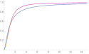
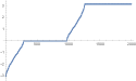
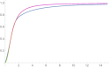
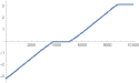
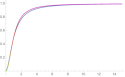
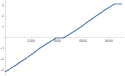
Figure 6. Radial and angle distributions of level crossings with $A$ and $B$ sampled from $GE^{{\mathbb{R}}}_{n}$ with $n=2,5,10$ approaching that of the uniform distribution on $\mathbb{C}P^{{1}}$. (The limiting theoretical radial density is shown by the magenta line and the experimental results by the blue line.)

We have also numerically evaluated the number of real level crossings among the total number of level crossings. (Real level crossing are represented by the horizontal segments of the graphs in the right column of Fig. 6.) Our numerics suggests that for a given size $n$, the average number of real level crossings is close to $\sqrt{n(n-1)}$ which is the square root of the total number of level crossings (given by $n(n-1)$). (Observe that in many similar situations involving real random univariate polynomials it is known that the average number of real roots equals the square root of their degree. Unfortunately, our situation is not covered by the known theoretical results.) We can prove that $\sqrt{2}$ is the expected average for $n=2$, see Lemma 4. For $n=3,4,5$ with 10000 samples, the quotient of the empirical average divided by $\sqrt{n(n-1)}$ was $1.0405,1.0404,1.04957$ resp. For $n=6$ with 5000 samples, the same quotient was $1.05586$ and, finally, for $n=10$ with 130 samples, the quotient was $1.06382$.

The structure of the paper is as follows. In § 2 we prove some general introductory results and make conclusions about the complex Gaussian ensembles. In § 3, we discuss the $SO_{2}$-action on $\mathbb{C}P^{{1}}$ and Gaussian ensembles. In § 4, we consider the cases of orthogonal Gaussian ensembles and Gaussian unitary ensembles and settle Theorems 2 and  3. In § 5, we settle Propositions 1 and 2 for the real Gaussian ensemble. Finally, in § 6, we present interesting numerical results about the monodromy statistics of $3\times 3$ linear families (1.1).

Acknowledgement.

B.S. wants to thank the Department of Mathematics of UIUC and, especially, Professor Y. Baryshnikov for the hospitality in June-July 2015 when a part of this project was carried out. The research of K.Z. was supported by the Marie Curie network GATIS of the European Union’s FP7 Programme under REA Grant Agreement No 317089, by the ERC advanced grant No 341222, by the Swedish Research Council (VR) grant 2013-4329, and by RFBR grant 18-01-00460.

2. $SU_{2}$-action and complex Gaussian ensembles

To prove our results about complex Gaussian ensembles, we need the following construction. The $GE_{n}^{{\mathbb{C}}}$-probability measure $\gamma:=\gamma_{GE_{n}^{{\mathbb{C}}}}$ on $Mat_{n}^{{\mathbb{C}}}$ induces the product probability measure $\gamma^{{(2)}}$ on $Mat_{n}^{{\mathbb{C}}}\times Mat_{n}^{{\mathbb{C}}}$. Consider the spectral determinant $\mathfrak{D}_{n}\subset Mat_{n}^{{\mathbb{C}}}\times Mat_{n}^{{\mathbb{C}}}\times\mathbb{C},$ which is a complex algebraic hypersurface consisting of all triples $(A,B,\lambda)$ such that the matrix $A+\lambda B$ has a multiple eigenvalue. Projection $\pi_{n}:\mathfrak{D}_{n}\to Mat_{n}^{{\mathbb{C}}}\times Mat_{n}^{{\mathbb{C}}}$ by forgetting the last coordinate induces a branched covering of $Mat_{n}^{{\mathbb{C}}}\times Mat_{n}^{{\mathbb{C}}}$ by $\mathfrak{D}_{n}$ of degree $n(n-1)$ whose fiber over a pair $(A,B)$ coincides with level crossing set of the linear family $A+\lambda B$. Taking the pullback $\pi^{{-1}}_{n}(\gamma^{{(2)}}),$ we obtain the probability measure $\Gamma:=\Gamma_{GE_{n}^{{\mathbb{C}}}}$ on $\mathfrak{D}_{n}$. (In other words, for any open subset $\mathcal{O}\subset\mathcal{D}_{n}$ which projects diffeomorphically on its image, $\Gamma(\mathcal{O})=\frac{1}{n(n-1)}\gamma(\pi_{n}(\mathcal{O}))$. Similar construction can be used for any branched covering whose base is equipped with an arbitrary probability measure.)

Now let $\kappa_{n}:\mathfrak{D}_{N}\to\mathbb{C}$ be the projection of the spectral determinant onto the last coordinate in $Mat_{n}^{{\mathbb{C}}}\times Mat_{n}^{{\mathbb{C}}}\times\mathbb{C}$, i.e., onto the $\lambda$-plane. Then the measure $\mu:=\mu_{GE_{n}^{{\mathbb{C}}}}$ we are looking for, coincides with the pushforward $\mu:=\kappa_{n}(\pi^{{-1}}_{n}(\gamma^{{(2)}}))$. (In other words, the value of measure $\mu$ on any measurable subset of $\mathbb{C}$ equals the value of measure $\Gamma$ of its complete preimage in $\mathcal{D}_{n}$.)

For our purposes, it will be more convenient to consider the space $Mat_{n}^{{\mathbb{C}}}\times Mat_{n}^{{\mathbb{C}}}\times\mathbb{CP}^{{1}},$ with the inclusion $\mathbb{C}\subset\mathbb{CP}^{{1}}$ given by the stereographic projection introduced in Remark 2. In other words, we use $\lambda:=b/a$, $(a:b)$ being the homogeneous coordinates on $\mathbb{CP}^{{1}}$. The above constructions work equally well on $Mat_{n}^{{\mathbb{C}}}\times Mat_{n}^{{\mathbb{C}}}\times\mathbb{CP}^{{1}}$ and provide us with the measure $\mu$ supported on $\mathbb{CP}^{{1}}$. (By a slight abuse of notation we denote both measures by the same letter.)

Consider the following $SU_{2}$-action on $Mat_{n}^{{\mathbb{C}}}\times Mat_{n}^{{\mathbb{C}}}$. A matrix $\mathfrak{U}\in SU_{2}$ given by $\begin{pmatrix}u&-\bar{v}\\ v&\bar{u}\end{pmatrix},\;$ $|u|^{{2}}+|v|^{{2}}=1$ acts on the latter product space by:

$$(A,B)\ast\mathfrak{U}\mapsto(uA+vB,-\bar{v}A+\bar{u}B).$$ (2.1)

Consider the following $SU_{2}$-action on $Mat_{n}^{{\mathbb{C}}}\times Mat_{n}^{{\mathbb{C}}}\times\mathbb{CP}^{{1}}$ extending the above action (2.1).
A matrix $\mathfrak{U}=\begin{pmatrix}u&-\bar{v}\\ v&\bar{u}\end{pmatrix},\;$ $|u|^{{2}}+|v|^{{2}}=1$ acts on $Mat_{n}^{{\mathbb{C}}}\times Mat_{n}^{{\mathbb{C}}}\times\mathbb{CP}^{{1}}$ by:

$$(A,B,a:b)\ast\mathfrak{U}\;\mapsto(uA+vB,-\bar{v}A+\bar{u}B,\bar{u}a+\bar{v}b:-va+ub).$$ (2.2)

Observe that the third component of the latter action coincides with the standard $SU_{2}$-action on a point $(a:b)\in\mathbb{CP}^{{1}}$ of the conjugate matrix $\begin{pmatrix}\bar{u}&-v\\ \bar{v}&u\end{pmatrix}\;$.

To prove Theorem 1 stated in the Introduction, we will show that $\mu$ is invariant under the above $SU_{2}$-action on $\mathbb{CP}^{{1}}.$ Since this action preserves the standard Fubini-Study metric on $\mathbb{C}P^{{1}},$ we can conclude that its density is constant with respect to the area form induced by the Fubini-Study metric, i.e., the one which has constant density in the cylindrical coordinates $(\phi,Z)$.

Our proof of Theorem 1 consists of three steps. On step 1 we will show that the action (2.2) on $Mat_{n}^{{\mathbb{C}}}\times Mat_{n}^{{\mathbb{C}}}\times\mathbb{CP}^{{1}}$ preserves the spectral determinant $\widehat{\mathfrak{D}}_{n}\subset Mat_{n}^{{\mathbb{C}}}\times Mat_{n}^{{\mathbb{C}}}\times\mathbb{CP}^{{1}}$. On step 2 we will prove that this action preserves the probability measure $\gamma^{{(2)}}$ on $Mat_{n}^{{\mathbb{C}}}\times Mat_{n}^{{\mathbb{C}}}$. As a consequence of steps 1 and 2, it also preserves the probability measure $\pi_{n}^{{-1}}(\gamma^{{(2)}})$ on $\widehat{\mathfrak{D}}_{n}$. On step 3 we will show the equivariance of (2.2) with respect to the projections $\pi_{n}$ and $\kappa_{n}$.

Lemma 1.

The action (2.2) preserves $\widehat{\mathfrak{D}}_{n}\subset Mat_{n}^{{\mathbb{C}}}\times Mat_{n}^{{\mathbb{C}}}\times\mathbb{CP}^{{1}}$.

Proof.

Take an arbitrary triple $(A,B,a:b)$ belonging to $\widehat{\mathfrak{D}}_{n}$, i.e., such that $aA+bB$ has a multiple eigenvalue, and take any $\mathfrak{U}=\begin{pmatrix}u&-\bar{v}\\ v&\bar{u}\end{pmatrix}\in SU_{2}$. We need to show that the triple

$$(uA+vB,-\bar{v}A+\bar{u}B,\bar{u}a+\bar{v}b:-va+ub)$$

also belongs to $\widehat{\mathfrak{D}}_{n}$. In other words, we need to check that if $aA+bB$ has a multiple eigenvalue, then the matrix

$$(\bar{u}a+\bar{v}b)(uA+vB)+(-va+ub)(-\bar{v}A+\bar{u}B)$$

has a multiple eigenvalue as well. The latter claim is obvious since expanding the above expression, we get $aA+bB$. ∎

Proof of Theorem 1.

To settle step 2, observe that in case of the $GE_{n}^{{\mathbb{C}}}$-ensemble, the probability density to obtain a matrix $A\in Mat_{n}^{{\mathbb{C}}}$ is given by:

$$\gamma(A)=\frac{1}{\pi^{{n^{{2}}}}}e^{{-\sum_{i,j=1}^{{n}}|A_{ij}|^{{2}}}}=\frac{1}{\pi^{{n^{{2}}}}}e^{{-Tr(AA^{{\star}})}},$$

where $A^{{\star}}$ stands for the conjugate-transpose of $A$. Therefore the density of $\gamma^{{(2)}}$ on $Mat_{n}^{{\mathbb{C}}}\times Mat_{n}^{{\mathbb{C}}}$ is given by:

$$\gamma^{{(2)}}(A,B)=\frac{1}{\pi^{{2n^{{2}}}}}e^{{-Tr(AA^{{\star}}+BB^{{\star}})}}.$$

Setting $C=uA+vB$ and $D=-\bar{v}A+\bar{u}B$, we get the relation

$$Tr(CC^{{\star}}+DD^{{\star}})=Tr(AA^{{\star}}+BB^{{\star}})=$$

$$=Tr(u\bar{u}AA^{{\star}}+v\bar{u}BA^{{\star}}+u\bar{v}AB^{{\star}}+v\bar{v}BB^{{\star}}+v\bar{v}AA^{{\star}}-\bar{u}vBA^{{\star}}-u\bar{v}AB^{{\star}}+u\bar{u}BB^{{\star}}).$$

The latter equality implies that the action (2.2) restricted to $Mat_{n}^{{\mathbb{C}}}\times Mat_{n}^{{\mathbb{C}}}$ (i.e., forgetting its action on the last coordinate $\mathbb{C}P^{{1}}$) preserves $\gamma^{{(2)}}$. By Lemma 1, the action (2.2) preserves the hypersurface $\widehat{\mathfrak{D}}_{n}$ and, therefore it preserves the probability measure $\pi_{n}^{{-1}}(\gamma^{{(2)}})$ on it.

To settle step 3, we need to show that the measure $\mu:=\kappa_{n}(\pi^{{-1}}_{n}(\gamma^{{(2)}}))$ on $\mathbb{C}P^{{1}}$ is invariant under the conjugate action of $SU_{2}$ on $\mathbb{C}P^{{1}}$, see the last component of (2.2). Take an arbitrary open set $\Omega\subset\mathbb{C}P^{{1}}$ and $g\in SU_{2}$. Denote by $g\cdot\Omega\subset\mathbb{C}P^{{1}}$ the shift of $\Omega$ by the conjugate of $g$. We need to prove that $\mu(\Omega)=\mu(g\cdot\Omega)$. By definition, $\mu(\Omega):=\pi^{{-1}}(\gamma^{{(2)}})(\kappa_{n}^{{-1}}(\Omega))$ and $\mu(g\cdot\Omega):=\pi^{{-1}}(\gamma^{{(2)}})(\kappa_{n}^{{-1}}(g\cdot\Omega))$. (Observe that both $\kappa_{n}^{{-1}}(\Omega)$ and $\kappa_{n}^{{-1}}(g\cdot\Omega)$ are measurable subsets of $\widehat{\mathfrak{D}}_{n}$.) Let us show that the (2.2)-action by $g$ sends $\kappa_{n}^{{-1}}(\Omega)$ to $\kappa_{n}^{{-1}}(g\cdot\Omega)$ and the (2.2)-action by the inverse $g^{{-1}}$ sends $\kappa_{n}^{{-1}}(g\cdot\Omega)$ to $\kappa_{n}^{{-1}}(\Omega)$ implying the required coincidence of measures due to step 2. Indeed $\kappa_{n}^{{-1}}(\Omega)$ is the set of all triples $(A,B,a:b)$ such that $aA+bB$ has a multiple eigenvalue and $(a:b)\in\Omega$. By Lemma 1, acting by $g$ on any such triple we get another triple $(\tilde{A},\tilde{B},\tilde{a}:\tilde{b})$ such that $\tilde{a}\tilde{A}+\tilde{b}\tilde{B}$ has a multiple eigenvalue and $(\tilde{a}:\tilde{b})\in g\cdot\Omega$. The same argument applies to the (2.2)-action by the inverse $g^{{-1}}$. ∎

Remark 6.

Observe that an alternative way to express the fact that the r.h.s. of (1.2) presents the constant density $\frac{1}{4\pi}$ with respect to the standard Euclidean area measure on $S^{{2}}\simeq\mathbb{C}P^{{1}}$ is as follows. Consider the standard cylindrical coordinate system $(\rho,\phi,Z)$ in $\mathbb{R}^{{3}},$ where $\rho\geq 0,0\leq\phi\leq 2\pi,Z\in\mathbb{R}$. Recall that

$$X=\rho\cos\phi,\;Y=\rho\sin\phi,\;Z=Z.$$

If we consider $(\phi,Z)$, $0\leq\phi\leq 2\pi,-1\leq Z\leq 1,$ as coordinates on the unit sphere $S^{{2}}\simeq\mathbb{C}P^{{1}}$ (with both poles removed), then in these coordinates the usual area element on the sphere is given by

$$dA=d\phi dZ.$$

Thus, in cylindrical coordinates $(\phi,Z)$, $0\leq\phi\leq 2\pi;\;-1\leq z\leq 1$ parameterising the unit sphere $S^{{2}}$, the measure $\mathcal{P}_{{GE}_{n}^{{\mathbb{C}}}}(x,y)dxdy$ given by (1.2) transforms into

$$\mathcal{P}_{{GE}_{n}^{{\mathbb{C}}}}(\phi,Z)d\phi dZ=\frac{d\phi dZ}{4\pi}.$$ (2.3)

In the case of $2\times 2$-matrices, the formula

$$\mathcal{P}_{GE_{2}^{{\mathbb{C}}}}(x,y)dxdy=\frac{1}{\pi\left(1+|\lambda|^{{2}}\right)^{{2}}}dxdy\,$$

can also be obtained by explicit calculations with the discriminantal equation similar to those in Sections 4 - 6.

Let us now present a number of generalisations of Theorem 1.

Proposition 3.

Conclusion of Theorem 1 holds, if $A$ and $B$ are independently chosen from the scaled complex Gaussian ensemble $GE_{\sigma^{{2}},n}^{{\mathbb{C}}},$ i.e., the ensemble whose off-diagonal entries are i.i.d. standard normal complex variables and whose diagonal entries are i.i.d. normal complex variables with an arbitrary fixed positive variance $\sigma^{{2}}$.

(In the above notation, $GE_{n}^{{\mathbb{C}}}=GE_{1,n}^{{\mathbb{C}}}.$)

The next observation together with Theorem 1 and Proposition 3 allows us to substantially extend the class of complex Gaussian ensembles whose distribution of level crossings is given by (1.2), i.e., it is uniform on $\mathbb{C}P^{{1}}$.

Take any complex linear subspace $W_{n}\subset Mat_{n}^{{\mathbb{C}}}$ such that the product space $W_{n}\times W_{n}\subset Mat_{n}^{{\mathbb{C}}}\times Mat_{n}^{{\mathbb{C}}}$ is preserved by the action (2.1). Given $\sigma>0$, denote by $W_{\sigma^{{2}},n}$ the space $W_{n}$ with the measure induced from the scaled complex Gaussian ensemble $GE_{\sigma^{{2}},n}^{{\mathbb{C}}}$.

Proposition 4.

In the above notation, level crossings of (1.1) with the random matrices $A$ and $B$ independently chosen from $W_{\sigma^{{2}},n}$ are uniformly distributed on $\mathbb{C}P^{{1}},$ i.e., their probability measure is given by the right-hand side of (1.2).

To give an example of such $W$, recall that $GOE_{n}^{{\mathbb{C}}}$ is the distribution on the space $Sym_{n}^{{\mathbb{C}}}$ of complex-valued symmetric matrices, where each entry $e_{i,j}=e_{j,i},\;i<j$ of a $n\times n$-matrix has a normal distribution $N(0,1/2)+iN(0,1/2)$, and each diagonal entry $e_{i,i}$ is distributed as $\sqrt{2}(N(0,1/2)+iN(0,1/2))$. Observe that $GOE_{n}^{{\mathbb{C}}}$ is obtained by restriction of $GE_{2,n}^{{\mathbb{C}}}$ to $Sym_{n}^{{\mathbb{C}}}$. (Discussions of general spectral properties of complex symmetric matrices can be found in e.g., [RaGaPrPu].)

Corollary 1.

Conclusion of Proposition 4 holds if $A$ and $B$ are independently chosen from the ensemble $GOE_{n}^{{\mathbb{C}}},$ and, more generally, from the scaled ensemble $GOE_{\sigma^{{2}},n}^{{\mathbb{C}}}$ whose off-diagonal entries are the i.i.d. standard symmetric normal complex variables and whose diagonal entries are the i.i.d. normal complex variables with an arbitrary fixed positive variance $\sigma^{{2}}$.

Remark 7.

Further interesting examples of linear subspaces $W$ covered by Proposition 4 include Toeplitz matrices, band matrices, band Toeplitz matices, diagonal matrices, etc.

Proof of Proposition 3.

In the set-up of this Proposition, the density of the probability to obtain a given matrix $A\in Mat_{n}^{{\mathbb{C}}}$ with respect to the Lebesgue measure is given by the formula

$$\widetilde{\gamma}(A)=Ke^{{-\sum_{i\neq j}|A_{ij}|^{{2}}-W\sum_{i=1}^{{n}}|A_{ii}|^{{2}}}}=Ke^{{-Tr(AA^{{\star}})-W\sum_{i=1}^{{n}}|A_{ii}|^{{2}}}},$$

where $K$ is a normalisation constant and $W$ is a real number. (To present a probability density in the above formula, the quadratic form $Tr(AA^{{\star}})+W\sum_{i=1}^{{n}}|A_{ii}|^{{2}}$ has to be positive-definite which implies that $W$ can not be a large negative number.) Therefore

$$\widetilde{\gamma}^{{(2)}}(A,B)=K^{{2}}e^{{-Tr(AA^{{\star}}+BB^{{\star}})-W\sum_{i=1}^{{n}}(|A_{ii}|^{{2}}+|B_{ii}|^{{2}})}}.$$ (2.4)

All we need to show is that the right-hand side of (2.4) is preserved under the action (2.2). In notation of the previous proof, we already know that $Tr(CC^{{\star}}+DD^{{\star}})=Tr(AA^{{\star}}+BB^{{\star}})$. It remains to prove that

$$\sum_{i=1}^{{n}}(|A_{ii}|^{{2}}+|B_{ii}|^{{2}})=\sum_{i=1}^{{n}}(|C_{ii}|^{{2}}+|D_{ii}|^{{2}}).$$

In fact, $|A_{ii}|^{{2}}+|B_{ii}|^{{2}}=|C_{ii}|^{{2}}+|D_{ii}|^{{2}}$ for each $i$ which follows from the relation

$$|C_{ii}|^{{2}}+|D_{ii}|^{{2}}=(uA_{ii}+vB_{ii})(\bar{u}\bar{A}_{ii}+\bar{v}\bar{B}_{ii})+(-\bar{v}A_{ii}+\bar{u}B_{ii})(-v\bar{A}_{ii}+u\bar{B}_{ii})=|A_{ii}|^{{2}}+|B_{ii}|^{{2}}.$$

∎

Proof of Proposition 4.

Repeats the above proof of Proposition 3. ∎

Proof of Corollary 1 .

Both statements follow from the observation that the action (2.2) preserves the subspace $Sym_{n}^{{\mathbb{C}}}\times Sym_{n}^{{\mathbb{C}}}\subset Mat_{n}^{{\mathbb{C}}}\times Mat_{n}^{{\mathbb{C}}}$ and that, additionally, the probability measure of the ensemble $GOE_{\sigma^{{2}},n}^{{\mathbb{C}}}$ (supported on $Sym_{n}^{{\mathbb{C}}}\times Sym_{n}^{{\mathbb{C}}}$) is induced from that of $GE_{(\sigma^{{\prime}})^{{2}},n}^{{\mathbb{C}}}$ for appropriate $\sigma^{{\prime}}$. ∎

3. $SO_{2}$-action for $GOE$-, $GUE$- and $GE^{{\mathbb{R}}}$-ensembles

This section provides some preliminary material for our study of level crossings of (1.1) with $A$ and $B$ chosen from the $GOE$-, $GUE$- and $GE^{{\mathbb{R}}}$-ensembles. A very essential feature of all these cases is that their level crossings distribution is invariant under the action of the subgroup $SO_{2}\subset SU_{2}$ given by the same formula (2.1), but with real $u$ and $v$ satisfying $u^{{2}}+v^{{2}}=1$, see Lemma 2.

In the above realization of $\mathbb{C}P^{{1}}$ as the unit sphere $S^{{2}}\subset\mathbb{R}^{{3}}$, $SO_{2}$ acts on it by rotation around the $Y$-axis, see Figure 7 and Lemma 2 below. This circumstance implies that the family of orbits of the $SO_{2}$-action on the unit sphere $S^{{2}}\simeq\mathbb{C}P^{{1}}$ projected to the complex plane of parameter $\lambda=x+iy$ will coincide with the family of circles given by

$$x^{{2}}+(y-t)^{{2}}=t^{{2}}-1,\quad|t|\geq 1.$$

Besides the above cylindrical coordinates $(\rho,\phi,Z)$ in $\mathbb{R}^{{3}}$, let us introduce the cylindrical coordinates $(\rho,\psi,Y)$ where $X=\rho\cos\psi,\;Y=Y,\;Z=\rho\sin\psi$. Then $(\psi,Y)$, $0\leq\psi\leq 2\pi,\;-1\leq Y\leq 1$ again parameterises the unit sphere $S^{{2}}\simeq\mathbb{C}P^{{1}}$. Lemma 2 implies that in the cylindrical coordinates $(\psi,Y)$, the distributions of level crossings of the above ensembles on $\mathbb{C}P^{{1}}$ are of the form:

$$dens(\psi,Y)d\psi dY=\rho(Y)d\psi dY,$$

for some univariate function $\rho$, i.e., its density depends only on $Y$ and is independent of the angle variable $\psi$. (In general, $\rho(Y)dY$ can be a $1$-dimensional measure which does not have a smooth density function. This happens, for example, in the case of $GE_{2}^{{\mathbb{R}}}$, when $\rho(Y)dY$ has a point mass at the origin.) In the original coordinates $(x,y)$, where $\lambda=x+iy$, the distribution of level crossings for the above cases will be of the form

$$dens(x,y)dxdy=\rho\left(\frac{2y}{x^{{2}}+y^{{2}}+1}\right)\frac{4dxdy}{(x^{{2}}+y^{{2}}+1)^{{2}}},$$ (3.1)

with the same $\rho$ as above, see Proposition 5.

Therefore the problem of finding the distribution of level crossings for Gaussian orthogonal, Gaussian unitary, and real Gaussian ensembles becomes in a sense one-dimensional which is a big advantage. In the cases under consideration, $\rho$ has an additional property of being an even function.

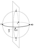
Figure 7. The $SO_{2}$-action on $\mathbb{C}P^{{1}}$ projectivising the complex plane of parameter $\lambda$ for the Gaussian orthogonal, Gaussian unitary, and real Gaussian ensembles.

We start with the following statement generalizing Lemma 1.

Lemma 2.

The action of $\mathcal{U}=\begin{pmatrix}u&-v\\ v&u\end{pmatrix}\in SO_{2}\subset SU_{2}$ on pairs of matrices $(A,B)$ given by

$$(A,B)\ast\begin{pmatrix}u&-v\\ v&u\end{pmatrix}=(uA+vB,-vA+uB),$$

where $u$ and $v$ are real numbers satisfying the condition $u^{{2}}+v^{{2}}=1$, preserves the following measures on the following matrix (sub)spaces:

a) the product $\gamma_{GOE}^{{(2)}}$ of two $GOE_{n}$-measures $\gamma_{GOE}$ on the space $Sym_{n}^{{\mathbb{R}}}\times Sym_{n}^{{\mathbb{R}}}$;

b) the product $\gamma_{GUE}^{{(2)}}$ of two $GUE_{n}$-measures $\gamma_{GUE}$ on the space $\mathcal{H}_{n}\times\mathcal{H}_{n}$;

c) the product $\gamma_{GE}^{{(2)}}$ of two $GE_{n}^{{\mathbb{R}}}$-measures $\gamma_{GE}$ on the space $Mat_{n}^{{\mathbb{R}}}\times Mat_{n}^{{\mathbb{R}}}$.

Proof.

Similarly to Lemma 1, $SO_{2}$ acts on $\widehat{\mathfrak{D}}_{n}\subset Sym_{n}^{{\mathbb{R}}}\times Sym_{n}^{{\mathbb{R}}}\times\mathbb{CP}^{{1}}$ (resp. on $\widehat{\mathfrak{D}}_{n}\subset\mathcal{H}_{n}\times\mathcal{H}_{n}\times\mathbb{CP}^{{1}}$ and on $\widehat{\mathfrak{D}}_{n}\subset Mat_{n}^{{\mathbb{R}}}\times Mat_{n}^{{\mathbb{R}}}\times\mathbb{CP}^{{1}}$), where $\widehat{\mathfrak{D}}_{n}$ is the spectral determinant, i.e., the set of all triples $\left(A,B,(a:b)\right)$ such that $(a:b)$ is a level crossing point of the pair $(A,B)$. (By a slight abuse of notation, in all cases we use the same letter for the spectral determinant.) Here $SO_{2}$ acts on $\mathbb{C}P^{{1}}$ as

$$(a:b)\ast\begin{pmatrix}u&-v\\ v&u\end{pmatrix}=(ua+vb:-va+ub).$$

Notice that $(ua+vb:-va+ub)$ is a level crossing point of the pair $(uA+vB,-vA+aB)$. Indeed,

$$(ua+vb)(uA+vB)+(-va+ub)(-vA+uB)=$$

$$=u^{{2}}aA+v^{{2}}bB+auvB+bvuA+v^{{2}}aA+u^{{2}}bB-auvB-bvuA=aA+bB.$$

Hence $SO_{2}$ acts on $\widehat{\mathfrak{D}}_{n}$, and this action commutes with the projections $\pi_{n}:\widehat{\mathfrak{D}}_{n}\to Sym_{n}^{{\mathbb{R}}}\times Sym_{n}^{{\mathbb{R}}}$ (resp. $\pi_{n}:\widehat{\mathfrak{D}}_{n}\to\mathcal{H}_{n}\times\mathcal{H}_{n}$ , and $\pi_{n}:\widehat{\mathfrak{D}}_{n}\to Mat_{n}^{{\mathbb{R}}}\times Mat_{n}^{{\mathbb{R}}}$), as well as with $\kappa_{n}:\widehat{\mathfrak{D}}_{n}\to\mathbb{C}P^{{1}}$. To check that the action of $SO_{2}$ on $Sym_{n}^{{\mathbb{R}}}\times Sym_{n}^{{\mathbb{R}}}$, $\mathcal{H}_{n}\times\mathcal{H}_{n}$, and $Mat_{n}^{{\mathbb{R}}}\times Mat_{n}^{{\mathbb{R}}}$, preserves the densities $\gamma_{GOE}^{{(2)}}$, $\gamma_{GUE}^{{(2)}}$, and $\gamma^{{(2)}}_{GE}$, respectively, recall that these densities are given by $C_{GOE_{n}}e^{{\frac{-n}{4}tr(A^{{2}}+B^{{2}})}}$, $C_{GUE_{n}}e^{{\frac{-n}{2}tr(AA^{{*}}+BB^{{*}})}}$, and $C_{GE_{n}}e^{{\frac{-n}{2}tr(AA^{{T}}+BB^{{T}})}}$, respectively. Here $C_{GOE_{n}},C_{GUE_{n}},C_{GE_{n}}$ are the corresponding normalising constants.

Therefore, in e.g., the orthogonal case, the density of the pair $(A,B)$ is determined by $tr(A^{{2}}+B^{{2}})$. At the same time

$$tr((uA+vB)^{{2}}+(-vA+uB)^{{2}})=$$

$$=tr(u^{{2}}A^{{2}}+uvAB+uvBA+v^{{2}}B^{{2}}+v^{{2}}A^{{2}}-uvAB-uvBA+u^{{2}}B)=tr(A^{{2}}+B^{{2}}).$$

Similar calculations work in the other two cases.

The density $\mu$ of level crossing points in $\mathbb{CP}^{{1}}$ is given by $\kappa_{n}\left(\pi_{n}^{{-1}}(\gamma_{GOE}^{{(2)}})\right)$ on $Sym_{n}^{{\mathbb{R}}}\times Sym_{n}^{{\mathbb{R}}}$, $\kappa_{n}\left(\pi_{n}^{{-1}}(\gamma_{GUE}^{{(2)}})\right)$ on $\mathcal{H}_{n}\times\mathcal{H}_{n}$, and $\kappa_{n}\left(\pi_{n}^{{-1}}(\gamma_{GE}^{{(2)}})\right)$ on $Mat_{n}^{{\mathbb{R}}}\times Mat_{n}^{{\mathbb{R}}}$ resp. That is, the measure $\mu$ of a measurable set $E\subset\mathbb{CP}^{{1}}$ is given by $\gamma^{{(2)}}(\pi_{n}(\kappa_{n}^{{-1}}(E)))$. Notice that

$$\mu(g\cdot E)=\gamma^{{(2)}}(\pi_{n}(\kappa_{n}^{{-1}}(g\cdot E)))=\gamma^{{(2)}}(\pi_{n}(g\cdot\kappa_{n}^{{-1}}(E)))=\gamma^{{(2)}}(g\cdot\pi_{n}(\kappa_{n}^{{-1}}(E)))=$$

$$=\gamma^{{(2)}}(\pi_{n}(\kappa_{n}^{{-1}}(E)))=\mu(E).$$

So we can conclude that for the above three ensembles, the density of level crossing points on $\mathbb{CP}^{{1}}$ is invariant under the above action by $SO_{2}$. ∎

Proposition 5.

In the standard coordinates $(X,Y,Z)$ in $\mathbb{R}^{{3}}$ introduced in Remark 2, the group $SO_{2}$ acts on $\mathbb{C}P^{{1}}\subset\mathbb{R}^{{3}}$ by rotation with respect to the $Y$-axis. This fact implies that in the above three cases, the distribution of level crossings in the cylindrical coordinates $(\psi;Y)$ is independent of $\psi$.

Proof.

We will show that for $\mathfrak{U}=\begin{pmatrix}\cos\Theta&-\sin\Theta\\ \sin\Theta&\cos\Theta\end{pmatrix}$, its action on a triple $(A,B,(\psi,Y))$ will be given by

$$(A,B,(\psi,Y))\ast\mathfrak{U}=(uA+vB,-vA+uB,(\psi+2\theta,Y))$$

implying that the action of $SO_{2}$ on $\mathbb{C}P^{{1}}$ realized as the unit sphere in $\mathbb{R}^{{3}}$ is by rotation of the sphere about the $Y$-axis. We only need to concentrate on the action of $\mathfrak{U}$ on the last coordinate. In the homogeneous coordinates $(a:b)$ of $\mathbb{C}P^{{1}}$, this action, by definition, is given by

$$(a:b)\ast\begin{pmatrix}\cos\Theta&-\sin\Theta\\ \sin\Theta&\cos\Theta\end{pmatrix}=(a\cos\Theta+b\sin\Theta:-a\sin\Theta+b\cos\Theta).$$

Setting $\lambda=\frac{a}{b}$ and $\lambda=x+iy$, we get that

$$\lambda_{\Theta}:=\lambda\ast\mathfrak{U}=\frac{\lambda\cos\Theta+\sin\Theta}{\cos\Theta-\lambda\sin\Theta}.$$

In terms of the pair $(x,y)$, the same action is expressed as

$$(x,u)\ast\mathfrak{U}:=(x_{\Theta},y_{\Theta})=$$

$$\left(\frac{(\sin\Theta+x\cos\Theta)(\cos\Theta-x\sin\Theta)-y^{{2}}\sin\Theta\cos\Theta}{(\cos\Theta-x\sin\theta)^{{2}}+(y\sin\Theta)^{{2}}},\frac{(\sin\Theta+x\cos\Theta)y\sin\Theta+(\cos\Theta-x\sin\Theta)y\cos\Theta}{(\cos\Theta-x\sin\theta)^{{2}}+(y\sin\Theta)^{{2}}}\right).$$

The relations between the coordinates $(x,y)$ in the $\lambda$-plane and the coordinates $(X,Y,Z)$ restricted to the sphere are as follows

$$X=x(1-Z)=\frac{2x}{x^{{2}}+y^{{2}}+1},\quad Y=y(1-Z)=\frac{2y}{x^{{2}}+y^{{2}}+1},\quad Z=\frac{x^{{2}}+y^{{2}}-1}{x^{{2}}+y^{{2}}+1}.$$ (3.2)

We have the relation

$$(\psi,Y)=\left(\arctan\frac{Z}{X},Y\right),$$

where $(X,Y,Z)$ are restricted to the sphere.

We need to express the above $SO_{2}$-action in the cylindrical coordinates $(\psi,Y)$ on $S^{{2}}\simeq\mathbb{C}P^{{1}}$. First we check that the coordinate $Y$ is preserved. In other words, for any real pair $(x,y)$, one forms the triple $(X,Y,Z)$ using (3.2). Then for the above pair $(x_{\Theta},y_{\Theta})$, one forms the triple $(X_{\Theta},Y_{\Theta},Z_{\Theta})$ using (3.2). What we need to check is that, for any $\Theta$, one has that $Y=Y_{\Theta}$. Indeed, $Y_{\Theta}$ is given by

$$Y_{\Theta}=2\frac{((xC+S)yS+(C-xS)yC)((C-xS)^{{2}}+(yS)^{{2}}}{Exp},$$

where $C:=\cos\Theta$, $S:=\sin\Theta$, and

$$Exp=((xC+S)^{{2}}(C-xS)^{{2}}-2y^{{2}}SC(xC+S)(C-xS)+y^{{2}}S^{{2}}C^{{2}}$$

$$+(xC+S)^{{2}}y^{{2}}S^{{2}}+2(xC+S)(C-xS)y^{{2}}SC+(C-xS)^{{2}}y^{{2}}C^{{2}}$$

$$+(C-xS)^{{4}}+2(C-xS)^{{2}}y^{{2}}S^{{2}}+y^{{4}}S^{{4}}.$$

Simplifying the above formula for $Y_{\Theta}$, we get

$$Y_{\Theta}=\frac{2y}{x^{{2}}+y^{{2}}+1}=Y.$$

Now we want to find the relation between the angle $\psi_{\Theta}$ and the pair $(\psi,\Theta)$. Observe that

$$\tan\psi_{\Theta}=\frac{Z_{\Theta}}{X_{\Theta}}=\frac{x_{\Theta}^{{2}}+y_{\Theta}^{{2}}-1}{2x_{\Theta}},$$

which using the above expressions for $(x_{\Theta},y_{\Theta})$ gives

$$\tan\psi_{\Theta}=\frac{((xC+S)(C-xS)-y^{{2}}SC)^{{2}}+((xC+S)yS+(C-xS)yC)^{{2}}-((C-xS)^{{2}}+y^{{2}}S^{{2}})^{{2}}}{2((C-xS)^{{2}}+y^{{2}}S^{{2}})((S+xC)(C-xS)-y^{{2}}SC)}.$$

Simplifyng the latter expression, we obtain

$$\tan\psi_{\Theta}=\frac{(x^{{2}}+y^{{2}}-1)\cos 2\Theta+2x\sin 2\Theta}{2x\cos 2\Theta-(x^{{2}}+y^{{2}}-1)\sin 2\Theta}=\frac{Z\cos 2\Theta+X\sin 2\Theta}{X\cos 2\Theta-Z\sin 2\Theta}.$$

Diving the numerator and denominator of the latter expression by $X\cos 2\Theta$, we get

$$\tan\psi_{\Theta}=\frac{\frac{Z}{X}+\tan 2\Theta}{1-\frac{Z}{X}\tan 2\Theta}=\frac{\tan\psi+\tan 2\Theta}{1-\tan\psi\tan 2\Theta}=\tan(\psi+2\Theta),$$

which implies that $\psi_{\Theta}=\psi+2\Theta$. ∎

Lemma 3.

If a smooth distribution which is invariant under the above $SO_{2}$-action is also radial in the $\lambda$-plane, then it is constant with respect to the spherical metric on $\mathbb{C}P^{{1}}$.

Proof.

Indeed, by formula (3.1), such a distribution in the $\lambda$-plane should be of the form

$$dens(x,y)dxdy=\rho\left(\frac{2y}{x^{{2}}+y^{{2}}+1}\right)\frac{4dxdy}{(x^{{2}}+y^{{2}}+1)^{{2}}}.$$

On the other hand, in the polar coordinates $(r,\theta)$ in the $\lambda$-plane, the same distribution has the form

$$den(r,\theta)drd\theta=R(r)drd\theta,$$

implying that

$$\rho\left(\frac{2y}{x^{{2}}+y^{{2}}+1}\right)\frac{4}{(x^{{2}}+y^{{2}}+1)^{{2}}}=\frac{R(r)}{r}\Leftrightarrow\rho\left(\frac{2y}{r^{{2}}+1}\right)=F(r).$$

The l.h.s is a function constant on the family of circles

$$x^{{2}}+(y-t)^{{2}}=t^{{2}}-1,\quad|t|\geq 1$$

while the r.h.s is constant on the family of circles

$$x^{{2}}+y^{{2}}=K$$

which can only happen when both sides are constant. Since $\rho\left(\frac{2y}{r^{{2}}+1}\right)=K$, the statement follows. ∎

4. Gaussian orthogonal ensembles and Gaussian unitary ensembles

Here we prove Theorems 2 and  3 stated in the Introduction. The main argument is similar to our other proofs dealing with the case $n=2$, comp. [ShZa1] and the next section; it has an advantage that one obtains more detailed information.

Notice that the ensemble $GOE_{n}$ is invariant under the conjugation by orthogonal matrices implying that for any pair of $GOE_{n}$-matrices $(A,B)$, we can conjugate $A+\lambda B$ by an orthogonal matrix to make $A$ diagonal.

Proof of Theorem 2.

By the above, we assume without loss of generality that $A$ is a diagonal matrix, i.e., $A=\left(\begin{array}[]{cc}\alpha_{1}&0\\ 0&\alpha_{2}\end{array}\right)$, where $\alpha_{1}$ and $\alpha_{2}$ are the eigenvalues of $A$ satisfying the condition $\alpha_{1}\leq\alpha_{2}$. Moreover, we can shift our matrix family so that $A=\left(\begin{array}[]{cc}0&0\\ 0&\Delta\end{array}\right)$, where $\Delta=\alpha_{2}-\alpha_{1}\geq 0$.

We know that level crossing points of the linear family $A+\lambda B$ are exactly the zeroes of the discriminant $Dsc(\lambda)$ of the characteristic polynomial $\chi(\lambda,t)$ with respect to the variable $t$, where

$$\chi(\lambda,t)=\text{det}(A+\lambda B+tI)=t^{{2}}+t(\lambda\;\mathrm{Tr}\,(B)+\Delta)+\lambda^{{2}}\det(B)+\lambda b_{11}\Delta.$$ (4.1)

The latter discriminant equals

$$Dsc(\lambda)=\lambda^{{2}}((b_{22}-b_{11})^{{2}}+4|b_{12}|^{{2}})+2\lambda\Delta(b_{22}-b_{11})+\Delta^{{2}}.$$ (4.2)

Therefore, since all coefficients of the latter equation are real and the discriminant of $Dsc(\lambda)$ considered as a quadratic equation in $\lambda$ is given by

$$D=-4\Delta^{{2}}|b_{12}|^{{2}}\leq 0,$$

level crossing points of a generic pair $(A,B)$ form a complex conjugate pair $(\lambda,\bar{\lambda})$, where

$$\lambda=\Delta\displaystyle\frac{b_{11}-b_{22}+2i|b_{12}|}{(b_{22}-b_{11})^{{2}}+4|b_{12}|^{{2}}}\quad\text{and}\quad\bar{\lambda}=\Delta\displaystyle\frac{b_{11}-b_{22}-2i|b_{12}|}{(b_{22}-b_{11})^{{2}}+4|b_{12}|^{{2}}}.$$ (4.3)

In order to find the distribution of $\lambda$, we will first find its conditional distribution assuming that $\Delta$ is constant. Set $\Sigma:=\frac{b_{11}-b_{22}}{\Delta}$ and $\Theta:=\frac{2|b_{12}|}{\Delta}$ giving $\lambda=\frac{1}{\Sigma-i\Theta}$.

Since $b_{11},b_{22}\sim N(0,2)$ and are independent, we get that $\Sigma\sim N(0,\frac{4}{\Delta^{{2}}})$. Further, $\Theta\sim\frac{2}{\Delta}|N(0,1)|$, which can be expressed using $\chi_{1}$-distribution, see e.g. [Chi]. Therefore, the conditional PDFs of $\Sigma$ and $\Theta$ are given by

$$\mathcal{P}_{\Sigma}^{{\Delta}}(u)=\frac{\Delta}{2\sqrt{2\pi}}\cdot e^{{-\frac{u^{{2}}\Delta^{{2}}}{8}}}$$

and

$$\mathcal{P}_{\Theta}^{{\Delta}}(v)=\begin{cases}\frac{\Delta}{\sqrt{2\pi}}\cdot e^{{-\frac{v^{{2}}\Delta^{{2}}}{8}}},\text{ for }v\geq 0;\\ 0,\quad\quad\quad\quad\text{otherwise.}\end{cases}$$

Since $\Sigma$ depends on $b_{11}$ and $b_{22}$, while $\Theta$ depends of $b_{12}$, we get that $\Sigma$ and $\Theta$ are independent random variables. Therefore, their joint distribution is given by

$$\mathcal{P}^{{\Delta}}_{(\Sigma,\Delta)}(u,v)=\mathcal{P}_{\Sigma}^{{\Delta}}(u)\cdot\mathcal{P}_{\Theta}^{{\Delta}}(v)=\begin{cases}\frac{\Delta^{{2}}}{4\pi}e^{{-\frac{\Delta^{{2}}(u^{{2}}+v^{{2}})}{8}}},\text{ for }\;v\geq 0;\\ 0,\quad\quad\quad\quad\quad\text{otherwise}.\end{cases}$$

Introduce $\mathfrak{X}:=\frac{\Sigma}{\Sigma^{{2}}+\Theta^{{2}}}$ and $\mathfrak{Y}:=\frac{\Theta}{\Sigma^{{2}}+\Theta^{{2}}}$ implying that $\lambda=\frac{1}{\Sigma-i\Theta}=\mathfrak{X}+i\mathfrak{Y}$. Since the Jacobian of the variable change is given by

$$\left|\frac{\partial(x,y)}{\partial(u,v)}\right|=\frac{1}{(u^{{2}}+v^{{2}})^{{2}}}=(x^{{2}}+y^{{2}})^{{2}},$$

the joint distribution of $\mathfrak{X}$ and $\mathfrak{Y}$ coincides with

$$\mathcal{P}_{(\mathfrak{X},\mathfrak{Y})}^{{\Delta}}(x,y)=\begin{cases}\frac{\Delta^{{2}}}{4\pi(x^{{2}}+y^{{2}})^{{2}}}\cdot e^{{-\frac{\Delta^{{2}}}{8(x^{{2}}+y^{{2}})}}},&\text{ for }\;y\geq 0;\\ 0,\quad\quad\quad\quad\quad&\text{otherwise}.\end{cases}$$

Therefore, the conditional distribution of $\lambda$ with $\Delta$ fixed equals

$$\mathcal{P}^{{\Delta}}(\lambda)=\frac{\Delta^{{2}}}{4\pi\mid\lambda\mid^{{4}}}\cdot e^{{-\frac{\Delta^{{2}}}{8\mid\lambda\mid^{{2}}}}},$$

The distribution of pairs of eigenvalues $(\alpha_{1},\alpha_{2})$ with $\alpha_{1}\leq\alpha_{2}$ of a $GOE_{2}$-matrix is given by

$$\mathcal{P}(\alpha_{1},\alpha_{2})=\frac{(\alpha_{2}-\alpha_{1})}{4\sqrt{2\pi}}\cdot e^{{-\frac{\alpha_{1}^{{2}}+\alpha_{2}^{{2}}}{4}}},$$

where $-\infty<\alpha_{1}\leq\alpha_{2}<\infty$.

Thus, the distribution of $\lambda$ with $\text{Im}\;\lambda>0$ is given by

$$\mathcal{P}_{>0}(\lambda) =\iint_{-\infty<\alpha_{1}\leq\alpha_{2}<\infty}\frac{(\alpha_{2}-\alpha_{1})}{4\sqrt{2\pi}}\cdot e^{{-\frac{\alpha_{1}^{{2}}+\alpha_{2}^{{2}}}{4}}}\cdot\frac{(\alpha_{2}-\alpha_{1})^{{2}}}{4\pi\mid\lambda\mid^{{4}}}\cdot e^{{-\frac{(\alpha_{2}-\alpha_{1})^{{2}}}{8\mid\lambda\mid^{{2}}}}}\ d\alpha_{2}\ d\alpha_{1}$$

$$=\iint_{-\infty<\alpha_{1}\leq\alpha_{2}<\infty}\frac{(\alpha_{2}-\alpha_{1})^{{3}}}{16\sqrt{2}\cdot\pi^{{3/2}}}\cdot\frac{1}{\mid\lambda\mid^{{4}}}\cdot e^{{-\frac{\alpha_{1}^{{2}}+\alpha_{2}^{{2}}}{4}}}\cdot e^{{-\frac{(\alpha_{2}-\alpha_{1})^{{2}}}{8\mid\lambda\mid^{{2}}}}}\ d\alpha_{2}\ d\alpha_{1}$$

$$=\frac{2}{\pi(1+\mid\lambda\mid^{{2}})^{{2}}}.$$

To get the actual PDF of $\lambda,$ we must divide the previous answer by $2$, getting

$$\mathcal{P}_{GOE_{2}}(\lambda)=\frac{1}{\pi(1+\mid\lambda\mid^{{2}})^{{2}}}.$$

∎

Now we consider the $2\times 2$-Gaussian unitary ensemble.

Proof of Theorem 3.

Using the same methods as for $GOE_{2}$, we calculated the distribution of level crossings for $GUE_{2}$-case. As in the previous case, level crossing point $\lambda$ with nonnegative imaginary part is given by

$$\lambda=\Delta\frac{b_{11}-b_{22}+2ib_{12}}{(b_{22}-b_{11})^{{2}}+4\mid b_{12}\mid^{{2}}}=\frac{1}{\Sigma-i\Theta},$$

where $\Sigma:=\frac{b_{11}-b_{22}}{\Delta}$ and $\Theta:=\frac{2\mid b_{12}\mid}{\Delta}$.

Since $b_{11},b_{22}\sim N(0,1)$ and are independent, we obtain $b_{22}-b_{11}\sim N(0,2)$, and hence, $\Sigma\sim N\left(0,\frac{2}{\Delta^{{2}}}\right)$. Therefore, the conditional PDF of $\Sigma$ is given by

$$\mathcal{P}_{\Sigma}^{{\Delta}}(u)=\frac{1}{\frac{\sqrt{2}}{\Delta}\sqrt{2}\sqrt{\pi}}e^{{-u^{{2}}\Delta^{{2}}/4}}=\frac{\Delta}{2\sqrt{\pi}}e^{{-u^{{2}}\Delta^{{2}}/4}}.$$

Since $\text{Re}(b_{12}),\text{Im}(b_{12})\sim N(0,\frac{1}{2})$, then $\frac{1}{1/\sqrt{2}}|b_{12}|\sim\chi_{2}$. Thus, the conditional PDF of $\Theta$ is given by

$$\mathcal{P}_{\Theta}^{{\Delta}}(v)=\begin{cases}\frac{\Delta^{{2}}y}{2}e^{{-v^{{2}}\Delta^{{2}}/4}},\text{ for }v\geq 0;\\ 0,\quad\quad\quad\quad\text{ otherwise.}\end{cases}$$

The joint distribution of $\Sigma$ and $\Theta$ gives us the conditional distribution of $\frac{1}{\lambda}$. Since $b_{12}$ is independent of $b_{11}$ and $b_{22}$, then $\Sigma$ and $\Theta$ are also independent random variables which implies that the conditional PDF of $\frac{1}{\lambda}$ is the product of the PDFs of $\Sigma$ and $\Theta$, i.e.,

$$\mathcal{P}_{1/\lambda}^{{\Delta}}(u,v)=\mathcal{P}_{\Sigma}^{{\Delta}}(u)\cdot\mathcal{P}_{\Theta}^{{\Delta}}(v)=\frac{\Delta^{{3}}}{4\sqrt{\pi}}ve^{{-(u^{{2}}+v^{{2}})\Delta^{{2}}/4}}.$$

Introducing $\mathfrak{X}:=\frac{\Sigma}{\Sigma^{{2}}+\Theta^{{2}}}$ and $\mathfrak{Y}:=\frac{\Theta}{\Sigma^{{2}}+\Theta^{{2}}}$, we get $\lambda=\frac{1}{\Sigma-i\Theta}=\mathfrak{X}+i\mathfrak{Y}$. Since the Jacobian of the variable change is given by

$$\left|\frac{\partial(x,y)}{\partial(u,v)}\right|=\frac{1}{(u^{{2}}+v^{{2}})^{{2}}}=(x^{{2}}+y^{{2}})^{{2}},$$

the joint distribution of $\mathfrak{X}$ and $\mathfrak{Y}$ coincides with

$$\mathcal{P}^{{\Delta}}_{(\mathfrak{X},\mathfrak{Y})}(x,y)=\frac{\mathcal{P}^{{\Delta}}_{\Sigma}(u)\cdot\mathcal{P}^{{\Delta}}_{\Theta}(v)}{\left|\frac{\partial(x,y)}{\partial(u,v)}\right|}=\frac{y\Delta^{{3}}e^{{-\Delta^{{2}}/4(x^{{2}}+y^{{2}})}}}{4\sqrt{\pi}(x^{{2}}+y^{{2}})^{{3}}}.$$

As $\mathfrak{X}=\text{Re}(\lambda)$ and $\mathfrak{Y}=\text{Im}(\lambda)$, then for a given value of $\Delta$, the conditional distribution of $\lambda$ is given by

$$\mathcal{P}^{{\Delta}}(\lambda)=\frac{\text{Im}(\lambda)\Delta^{{3}}e^{{-\Delta^{{2}}/4|\lambda|^{{2}}}}}{4\sqrt{\pi}|\lambda|^{{6}}}.$$

Finally, in order to find the (unconditional) distribution of $\lambda$, we recall that the PDF of the joint distribution for pairs of eigenvalues $\alpha_{1}\leq\alpha_{2}$ of a random matrix belonging to $GUE_{2}$ is given by

$$\mathcal{P}(\alpha_{1},\alpha_{2})=\frac{1}{2\pi}(\alpha_{2}-\alpha_{1})^{{2}}e^{{-(\alpha_{1}^{{2}}+\alpha_{2}^{{2}})/2}}=\frac{\Delta^{{2}}}{2\pi}e^{{-(\alpha_{1}^{{2}}+\alpha_{2}^{{2}})/2}}.$$

Therefore, since $\Delta=a_{2}-a_{1}$, the distribution for level crossing point $\lambda$ with $\text{Im}\;\lambda\geq 0$ is given by

$\mathcal{P}_{>0}(\lambda)$	$=\displaystyle\iint_{-\infty<a_{1}\leq a_{2}<+\infty}\mathcal{P}^{{\Delta}}(\lambda)\cdot\mathcal{P}(\alpha_{1},\alpha_{2})\ d\alpha_{2}\ d\alpha_{1}$
	$=\displaystyle\iint_{-\infty<a_{1}\leq a_{2}<+\infty}\frac{(\alpha_{2}-\alpha_{1})^{{5}}}{8\pi^{{3/2}}}\cdot\frac{\text{Im}(\lambda)}{|\lambda|^{{6}}}\cdot e^{{\frac{-(\alpha_{2}-\alpha_{2})^{{2}}}{4|\lambda|^{{2}}}-\frac{(\alpha_{1}^{{2}}+\alpha_{2}^{{2}})}{2}}}\ d\alpha_{2}\ d\alpha_{1}$
	$=\displaystyle\frac{8\text{Im}(\lambda)}{\pi(1+|\lambda|^{{2}})^{{3}}}.$

Therefore, the actual distribution for level crossing point $\lambda\in\mathbb{C}$ equals

$$\mathcal{P}_{GUE_{2}}(\lambda)=\displaystyle\frac{4|\text{Im}(\lambda)|}{\pi(1+|\lambda|^{{2}})^{{3}}}.$$

∎

5. Real Gaussian ensembles

In this section, in order to prove Propositions 1 and 2 stated in the Introduction, we will use the standard presentation of real $2\times 2$-matrices as linear combinations of Pauli matrices which was extensively applied in [ShZa1]. Namely, let $A=(a_{+},ia_{-},a_{\Delta})\cdot\vec{\sigma}$ be a real 2-by-2 matrix with normal variables, generic up to additional multiples of identity. Here $\vec{\sigma}=(\sigma_{1},\sigma_{2},\sigma_{3})$ is the standard triple of Pauli matrices. Denote the coefficient vector $(a_{+},a_{-},a_{\Delta})$ by $\vec{A}$ and consider the inner product on such triples using a Minkowski metric:

$$\vec{A}\cdot\vec{B}:=_{\text{def}}\vec{A}\begin{pmatrix}[c]1&0&0\\ 0&-1&0\\ 0&0&1\end{pmatrix}\vec{B}.$$ (5.1)

Notice that the discriminant of $A$, i.e., the expression which vanishes if and only $A$ has a multiple eigenvalue, is given by

$$D_{A}=\vec{A}\cdot\vec{A}=a_{+}^{{2}}-a_{-}^{{2}}+a_{\Delta}^{{2}}.$$ (5.2)

Similarly construct $B=(b_{+},ib_{-},b_{\Delta})\cdot\vec{\sigma}$ and consider the linear family

$$C=A+\lambda B.$$ (5.3)

We get

$$D_{C}=D_{A}+\lambda^{{2}}D_{B}+2\lambda\vec{A}\cdot\vec{B}$$ (5.4)

with zeroes at

$$\lambda=-\frac{\vec{A}\cdot\vec{B}}{D_{B}}\pm\sqrt{\left(\frac{\vec{A}\cdot\vec{B}}{D_{B}}\right)^{{2}}-\frac{D_{A}}{D_{B}}}.$$ (5.5)

Firstly, let us prove Proposition 1.

Proof.

To settle Part (i), observe that $\frac{\lambda_{+}+\lambda_{-}}{2}=-\frac{\vec{A}\cdot\vec{B}}{\vec{B}\cdot\vec{B}}$ which amounts to computing a single delta. In this case we make the isometric transformation $b_{-}\mapsto-b_{-}$ and let $a$ be the component of $\vec{A}$ along $\vec{B}$, which allows us to work in a Euclidean space for the purposes of computing $\vec{A}\cdot\vec{B}$. We also use spherical coordinates for $\vec{B}$ given by:

$$b_{+} =R_{B}\sin\phi_{B}\cos\theta_{B};$$ (5.6)

$$b_{\Delta} =R_{B}\sin\phi_{B}\sin\theta_{B};$$ (5.7)

$$b_{-} =-R_{B}\cos\phi_{B};$$ (5.8)

$$-\frac{\vec{A}\cdot\vec{B}}{D_{B}} =-\frac{aR_{B}}{R_{B}^{{2}}(1-2\cos^{{2}}\phi_{B})}=\frac{a}{R_{B}\cos(2\phi_{B})}.$$ (5.9)

Note that here $R_{B}^{{2}}$ is $\chi_{3}^{{2}}$-distributed whereas $r_{B}^{{2}}$ is $\chi_{2}^{{2}}$-distributed. Next observe that $c\equiv\cos\phi_{B}$ is uniformly distributed for any spherically symmetric distribution, which means that if $c=\pm\sqrt{\frac{1-t}{2}}$, then

$$\rho_{\cos\phi_{B}}(c)dc =\frac{dc}{2};$$ (5.10)

$$\rho_{1-2\cos^{{2}}\phi_{B}}(t)dt =\frac{2\left|\frac{d}{dt}\sqrt{\frac{1-t}{2}}\right|dt}{2}dt=\frac{dt}{2\sqrt{2-2t}};$$ (5.11)

$$R_{B}\propto\rho_{\sqrt{\chi_{3}^{{2}}}}(R) =\sqrt{\frac{2}{\pi}}R^{{2}}e^{{-R^{{2}}/2}}.$$ (5.12)

So the distribution of the average of two level crossings simply becomes

$$\rho_{\frac{\lambda_{+}+\lambda_{-}}{2}}(x)=\iiint\delta\left(x+\frac{a}{Rt}\right)\rho(a,R,t)dadRdt.$$ (5.13)

Resolving the delta with respect to $a$ gives $\left|\frac{da}{dx}\right|=|Rt|$ which implies that

$$\begin{split}\rho_{\frac{\lambda_{+}+\lambda_{-}}{2}}(x)&=\int_{-1}^{{1}}dt\int_{0}^{{\infty}}dR\left|R^{{3}}t\right|\frac{e^{{-\frac{R^{{2}}+(xtR)^{{2}}}{2}}}}{2\pi\sqrt{2-2t}}\\ &=\int_{-1}^{{1}}dt\int_{0}^{{\infty}}dR\frac{|t|}{2\pi\sqrt{2-2t}}R^{{3}}e^{{-(1+x^{{2}}t^{{2}})\frac{R^{{2}}}{2}}}\\ &=\int_{-1}^{{1}}\frac{\left|t\right|}{\pi\sqrt{2-2t}\left(x^{{2}}t^{{2}}+1\right)^{{2}}}dt.\end{split}$$ (5.14)

To settle Part (ii), compute the distribution of $D_{B}=(b_{+}^{{2}}+b_{\Delta}^{{2}})-b_{-}^{{2}}$:

$$\begin{split}\rho_{D}(D)&=\iint_{0}^{{\infty}}\delta(D+y-x)\rho_{\chi_{2}^{{2}}}(x)\frac{e^{{-y/2}}}{\sqrt{8\pi y}}dxdy\\ &=\frac{e^{{-D/2}}}{\sqrt{8}}\left(1-\Theta(-D)\text{erf}(\sqrt{-D})\right).\end{split}$$ (5.15)

It’s worth noting that in the positive range this is just $\frac{\rho_{\chi^{{2}}_{2}}(x)}{\sqrt{2}}$, so the probability that the discriminant is positive is $\frac{1}{\sqrt{2}}$.

The distribution of the product $\lambda_{+}\lambda_{-}=\frac{D_{A}}{D_{B}}$ is the $D$-ratio distribution:

$$\rho_{\lambda_{+}\lambda_{-}}(x)=\int_{-\infty}^{{\infty}}|y|\rho_{D}(y)\rho_{D}(xy)dy.$$ (5.16)

We split the latter integral into four parts depending on the signs of $x$ and $y$:

$$\rho_{++} =\int_{0}^{{\infty}}\frac{ye^{{-y(1+x)/2}}}{8}=\frac{1}{2(x+1)^{{2}}};$$ (5.17)

$$\rho_{+-} =\int_{-\infty}^{{0}}-\frac{ye^{{-y(1+x)/2}}}{8}\text{erfc}(\sqrt{-y})\text{erfc}(\sqrt{-xy});$$ (5.18)

$$\rho_{--} =\int_{-\infty}^{{0}}-\frac{ye^{{-y(1+x)/2}}}{8}\text{erfc}(\sqrt{-y})=\frac{1}{2(x+1)^{{2}}}\left(1+\frac{3x-1}{\sqrt{2}(1-x)^{{3/2}}}\right);$$ (5.19)

$$\rho_{-+} =\int_{0}^{{\infty}}\frac{ye^{{-y(1+x)/2}}}{8}\text{erfc}(\sqrt{-xy})=\frac{1}{2(x+1)^{{2}}}\left(1+\frac{(x-3)\sqrt{-x}}{\sqrt{2}(1-x)^{{3/2}}}\right).$$ (5.20)

Observe that only one integral out of four can not be computed in a closed form, but it can be computed numerically using e.g., Mathematica. Combining terms, we get

$$\begin{split}\rho_{\frac{D_{A}}{D_{B}}}(x)&=\Theta(x)\left[\frac{1}{2(x+1)^{{2}}}-\int_{-\infty}^{{0}}\frac{ye^{{-y(1+x)/2}}}{8}\text{erfc}(\sqrt{-y})\text{erfc}(\sqrt{-xy})dy\right]\\ &+\Theta(-x)\left[\frac{1}{(x+1)^{{2}}}\left(1+\frac{3x-1+(x-3)\sqrt{-x}}{\sqrt{8}(1-x)^{{3/2}}}\right)\right]\end{split}$$ (5.21)

which is the required expression. ∎

We now turn to Proposition 2.

Lemma 4.

If $A$ and $B$ are independently chosen from the $GE_{2}^{{\mathbb{R}}}$-ensemble, then the probability of attaining a real pair of level crossing points $\lambda_{\pm}$ in the family $C=A+\lambda B$ equals $\frac{1}{\sqrt{2}}$.

Proof.

We use a result from [ShZa1] saying that the proportion of real eigenvalues for a fixed $A$ is given by

$$\kappa(a_{+},a_{-},a_{\Delta})=\begin{cases}1&\text{if }D_{A}<0\\ 1-\frac{1}{\pi}\arccos\frac{a_{-}^{{2}}}{a_{+}^{{2}}+a_{\Delta}^{{2}}}&\text{if }D_{A}\geq 0,\end{cases}$$ (5.22)

see formula (5.43) in loc. cit. The expectation value over the set of matrices with positive discriminant is given by

$$\langle\kappa\rangle_{D_{A}\geq 0}=\iiint_{D_{A}\geq 0}\left(1-\frac{1}{\pi}\arccos\frac{a_{-}^{{2}}}{a_{+}^{{2}}+a_{\Delta}^{{2}}}\right)\rho(a_{+},a_{-},a_{\Delta})da_{+}da_{-}da_{\Delta}.$$ (5.23)

Using spherical coordinates relative to the $a_{-}$-axis we can simplify the integral as:

$$\int_{0}^{{\infty}}2\pi r^{{2}}\frac{e^{{-r^{{2}}/2}}}{(2\pi)^{{3/2}}}dr\int_{-\frac{1}{\sqrt{2}}}^{{\frac{1}{\sqrt{2}}}}\left(1-\frac{1}{\pi}\arccos\frac{\cos^{{2}}\phi}{1-\cos^{{2}}\phi}\right)d(\cos\phi)=\sqrt{2}-1.$$ (5.24)

On the other hand, the contribution of the set of matrices with $D_{A}<0$ is just

$$\langle\kappa\rangle_{D_{A}<0}=\iiint_{D_{A}<0}\rho(a_{+},a_{-},a_{\Delta})da_{+}da_{-}da_{\Delta}=P(D_{A}<0)=1-\frac{1}{\sqrt{2}}$$ (5.25)

where the last step follows from equation (5.15). Thus the total probability of getting a real crossing value is

$$\langle\kappa\rangle=\sqrt{2}-1+1-\frac{1}{\sqrt{2}}=\frac{1}{\sqrt{2}}.$$ (5.26)

∎

Let us now prove Proposition 2.

Proof.

Due to the isotropy of a normally distributed vector, we are free to rotate the coordinate system in the $(b_{+},b_{\Delta})$-plane such that $\vec{B}=(r_{B},b_{-},0)$. This $B$-dependent choice of a basis has no impact on the distribution of $\vec{A}$ which has the normally distributed entries $(a_{1},a_{-},a_{2})$ in this basis.

To settle Part (i) of the Proposition, assume that the level crossing points $\lambda_{\pm}=x\pm iy$ are complex conjugate, in which case we get

$$x =-\frac{\vec{A}\cdot\vec{B}}{\vec{B}\cdot\vec{B}}=\frac{a_{1}r_{B}-a_{-}b_{-}}{r_{B}^{{2}}-b_{-}^{{2}}};$$ (5.27)

$$y =\sqrt{\frac{D_{A}}{D_{B}}-\left(\frac{\vec{A}\cdot\vec{B}}{D_{B}}\right)^{{2}}}=\sqrt{\frac{a_{1}^{{2}}-a_{-}^{{2}}+a_{2}^{{2}}}{r_{B}^{{2}}-b_{-}^{{2}}}-x^{{2}}}.$$ (5.28)

Therefore the density of the joint distribution with respect to the Lebesgue measure in the plane takes the form

$$\rho(x,y)=\iiint_{A}\iiint_{B}\delta\left(x+\frac{a_{1}r_{B}-a_{-}b_{-}}{r_{B}^{{2}}-b_{-}^{{2}}}\right)\delta\left(y-\sqrt{\frac{a_{1}^{{2}}-a_{-}^{{2}}+a_{2}^{{2}}}{r_{B}^{{2}}-b_{-}^{{2}}}-x^{{2}}}\right)\rho(\vec{A},\vec{B}).$$ (5.29)

Resolving the first delta with respect to $a_{-}$, we get

$$a_{-} =\frac{a_{1}r_{B}+x(r_{B}^{{2}}-b_{-}^{{2}})}{b_{-}};$$ (5.30)

$$\left|\frac{da_{-}}{dx}\right| =\left|\frac{r_{B}^{{2}}-b_{-}^{{2}}}{b_{-}}\right|.$$ (5.31)

Then resolving the second delta with respect to $a_{2}^{{2}}$, we obtain

$$a_{2}^{{2}} =(r_{B}^{{2}}-b_{-}^{{2}})(x^{{2}}+y^{{2}})+\left(\frac{a_{1}r_{B}+x(r_{B}^{{2}}-b_{-}^{{2}})}{b_{-}}\right)^{{2}}-a_{1}^{{2}};$$ (5.32)

$$\left|\frac{d(a_{2}^{{2}})}{dy}\right| =\left|2y(r_{B}^{{2}}-b_{-}^{{2}})\right|.$$ (5.33)

Inserting, we get

$$\begin{split}\rho(x,y)=\int_{a_{1}}\iiint_{B}\left|\frac{2y}{b_{-}}(r_{B}^{{2}}-b_{-}^{{2}})^{{2}}\right|\rho_{a_{-}}\left(\frac{a_{1}r_{B}+x(r_{B}^{{2}}-b_{-}^{{2}})}{b_{-}}\right)\\ \cdot\rho_{a_{2}^{{2}}}((r_{B}^{{2}}-b_{-}^{{2}})(x^{{2}}+y^{{2}})+\left(\frac{a_{1}r_{B}+x(r_{B}^{{2}}-b_{-}^{{2}})}{b_{-}}\right)^{{2}}-a_{1}^{{2}})\\ \cdot\rho_{a_{1}}(a_{1})\rho_{r_{B}}(r_{B})\rho_{\theta_{B}}(\theta_{B})\rho_{b_{-}}(b_{-}).\end{split}$$ (5.34)

Expanding the expression and integrating out $\theta_{B}$ gives us:

$$\begin{split}\rho(x,y)=\int_{-\infty}^{{\infty}}da_{1}\int_{0}^{{\infty}}dr_{B}\int_{-\infty}^{{\infty}}db_{-}\left|\frac{2y}{b_{-}}(r_{B}^{{2}}-b_{-}^{{2}})^{{2}}\right|\frac{e^{{-\left(\frac{a_{1}r_{B}+x(r_{B}^{{2}}-b_{-}^{{2}})}{b_{-}}\right)^{{2}}/2}}}{\sqrt{2\pi}}\\ \cdot\frac{e^{{-((r_{B}^{{2}}-b_{-}^{{2}})(x^{{2}}+y^{{2}})+\left(\frac{a_{1}r_{B}+x(r_{b}^{{2}}-b_{-}^{{2}})}{b_{-}}\right)^{{2}}-a_{1}^{{2}})/2}}}{\sqrt{2\pi}\sqrt{(r_{B}^{{2}}-b_{-}^{{2}})(x^{{2}}+y^{{2}})+\left(\frac{a_{1}r_{B}+x(r_{B}^{{2}}-b_{-}^{{2}})}{b_{-}}\right)^{{2}}-a_{1}^{{2}}}}\\ \cdot\Theta\left[((r_{B}^{{2}}-b_{-}^{{2}})(x^{{2}}+y^{{2}})+\left(\frac{a_{1}r_{B}+x(r_{B}^{{2}}-b_{-}^{{2}})}{b_{-}}\right)^{{2}}-a_{1}^{{2}}\right]\\ \cdot\frac{e^{{-a_{1}^{{2}}/2}}}{\sqrt{2\pi}}r_{B}e^{{-r_{B}^{{2}}/2}}\frac{e^{{-b_{-}^{{2}}/2}}}{\sqrt{2\pi}}.\end{split}$$ (5.35)

After some extra simplifications, we get

$$\begin{split}\rho(x,y)=\int_{-\infty}^{{\infty}}da_{1}\int_{0}^{{\infty}}dr_{B}\int_{-\infty}^{{\infty}}db_{-}\left|\frac{yr_{B}}{2\pi^{{2}}b_{-}}(r_{B}^{{2}}-b_{-}^{{2}})^{{2}}\right|e^{{-\frac{a_{1}^{{2}}+r_{B}^{{2}}+b_{-}^{{2}}}{2}}}\\ \cdot\frac{e^{{-((r_{B}^{{2}}-b_{-}^{{2}})(x^{{2}}+y^{{2}})+\left(\frac{a_{1}r_{B}+x(r_{b}^{{2}}-b_{-}^{{2}})}{b_{-}}\right)^{{2}}-a_{1}^{{2}})/2}}}{\sqrt{(r_{B}^{{2}}-b_{-}^{{2}})(x^{{2}}+y^{{2}})+\left(\frac{a_{1}r_{B}+x(r_{B}^{{2}}-b_{-}^{{2}})}{b_{-}}\right)^{{2}}-a_{1}^{{2}}}}\\ \cdot\Theta\left[((r_{B}^{{2}}-b_{-}^{{2}})(x^{{2}}+y^{{2}})+\left(\frac{a_{1}r_{B}+x(r_{B}^{{2}}-b_{-}^{{2}})}{b_{-}}\right)^{{2}}-a_{1}^{{2}}\right].\end{split}$$ (5.36)

Suppressing the superfluous subscripts from the integration variables, we obtain the triple integral from the formulation of Proposition 2.

To settle Part (ii), observe that by formula (3.1), the density of a distribution the level crossings invariant under the $SO_{2}$-action on the real axis should be proportional to $\frac{1}{(1+x^{{2}})^{{2}}}$. By Lemma 4 the total mass of the measure of level crossings concentrated on the real axis equals $\frac{1}{\sqrt{2}}$. Using this normalization, we arrive at the expression (1.8). ∎

6. Monodromy distribution for $3\times 3$ Gaussian ensembles

In this section we present numerical results about the monodromy of random $3\times 3$ linear matrix families (1.1). Monodromy statistics was collected for the cases of $GUE_{3}$-, $GOE_{3}$-, and $GE_{3}^{{\mathbb{C}}}$-ensembles. (One can easily check that the number of possible monodromy sequences for the matrix sizes exceeding $3$ is so large that it is practically impossible to collect coherent statistical information numerically.) Some of the numerical results below are rather surprising, see Remark 8.

General observations. Observe that, for generic pairs of matrices $A$ and $B$ from $GUE_{n}$ and $GOE_{n}$, all level crossings are simple and arise in complex conjugate pairs; $\binom{n}{2}$ of them lying in the upper half-plane and $\binom{n}{2}$ lying symmetrically in the lower half-plane. We can additionally assume that all level crossings in the upper half-plane have distinct real parts since the coincidence of the real parts happens with probability $0$. Denote by $\lambda_{1},\lambda_{2},\dots,\lambda_{\binom{n}{2}}$ level crossing points in the upper half-plane ordered by the increase of their real parts. Since generically level crossing points are simple, let $\sigma_{1},\sigma_{2},\dots,\sigma_{\binom{n}{2}}$ be the associated sequence of transpositions obtained as follows, see Fig. 8. Under our assumptions, for every real $\lambda$, the spectrum of $A+\lambda B$ is real and simple which means that no monodromy of the spectrum occurs when $\lambda$ belongs to the real axis $\mathbb{R}\subset\mathbb{C}$.

If $\lambda_{i}$ is the $i$-th level crossing point in the upper half-plane in the order of increasing real parts, consider the path in the $\lambda$-plane starting on the real axis at $\tau=Re(\lambda_{i})$, going straight up to $\lambda_{i}$, making a small loop encircling $\lambda_{i}$ counterclockwise, and returning back to $\tau_{i}$. As a result, one gets a transposition $\sigma_{i}$ of two real eigenvalues corresponding to $\tau_{i}=Re(\lambda_{i})$. Doing this for each $\lambda_{i}$, $i=1,\dots,\binom{n}{2}$, we obtain a sequence of $\binom{n}{2}$ transpositions $\left(\sigma_{1},\sigma_{2},\ldots,\sigma_{\binom{n}{2}}\right)$, $\sigma_{i}\in S_{n}$.

One can easily check that the obtained sequence $\left(\sigma_{1},\sigma_{2},\ldots,\sigma_{\binom{n}{2}}\right)$ of transpositions satisfies the following two conditions:

(i) for general $A$ and $B$, they generate the symmetric group $S_{n}$;

(ii) the product $\sigma_{1}\cdot\sigma_{2}\cdot\ldots\cdot\sigma_{\binom{n}{2}}$ coincides with the inverse permutation $(n,n-1,\dots,1)$.

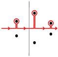
Figure 8. Creating the monodromy sequence

Notice that the statistics of the monodromy sequences of transpositions for $GUE_{n}$ and $GOE_{n}$ are invariant under conjugation by the inverse permutation $(n,n-1,\dots,1)$ as well as under reversing the order of the transpositions. These symmetries can be explained as consequences of the symmetries of the ensembles.

Namely, if the matrix $A+\lambda B$ has eigenvalues $\alpha_{1},\alpha_{2},\dots,\alpha_{n}$, then the matrix $-A-\lambda B$ has eigenvalues $-\alpha_{1},-\alpha_{2},\dots,-\alpha_{n}$. These matrix pencils share the same level crossing points, and if a loop in $\mathbb{CP}^{{1}}$ permutes the eigenvalues of $A+\lambda B$, then it applies the same permutation to the eigenvalues of $-A-\lambda B$. However, when we compute the monodromy associated to a pair of matrices in our ensembles, we order the (real) eigenvalues for real $\lambda$, and the transpositions associated to each level crossing point are written with respect to this ordering. Since the eigenvalues of $-A-\lambda B$ will have the ordering opposite to those of $A+\lambda B$, the monodromy associated to the pair $(-A,-B)$ will be the monodromy of $(A,B)$, conjugated by $(n,n-1,\dots,1)$. Since the pairs $(A,B)$ and $(-A,-B)$ have the same probability density, each of the admissible sequences of transpositions will appear with the same frequency as its conjugate.

The other symmetry of our data is its invariance under reversing the order of the transpositions. It can be similarly explained by the equal probability density for the pairs $(A,B)$ and $(A,-B)$. If level crossing points of $A+\lambda B$ are $\lambda_{1},\lambda_{2},\dots,\lambda_{n(n-1)}$, then level crossing points of $A-\lambda B$ are $-\lambda_{1},-\lambda_{2},\dots,-\lambda_{n(n-1)}$. Level crossing points come in conjugate pairs, and the same transpositions are associated to these pairs, so if $\lambda_{1},\lambda_{2},\dots,\lambda_{\binom{n}{2}}$ are level crossing points of $A+\lambda B$ in the upper half-plane, then $-\overline{\lambda}_{1},-\overline{\lambda}_{2},\dots,-\overline{\lambda}_{\binom{n}{2}}$ are level crossing points of $A-\lambda B$ in the upper half-plane. Since we order them according to the increase of their real parts, which have been inverted, it now remains to show that the transposition associated to $(A,B,\lambda_{i})$ is the same as that associated to $(A,-B,-\overline{\lambda}_{i})$. Since the transposition associated to level crossing point is the same as that associated to its conjugate, we can instead consider $(A,-B,-\lambda_{i})$. Observe that the transposition associated to $(A,B,\lambda_{i})$ is determined by the eigenvalues of

$$A+(Re(\lambda_{i})+\epsilon Im(\lambda_{i}))B$$

for $0\leq\epsilon\leq 1$, and in the same way the transposition associated to $(A,-B,-\lambda_{i})$ is determined by

$$A+(Re(-\lambda_{i})+\epsilon Im(-\lambda_{i}))(-B)=A+(Re(\lambda_{i})+\epsilon Im(\lambda_{i}))B.$$

These coincide, and we conclude that the monodromy sequence associated to $(A,-B)$ is the reverse of that associated to $(A,B)$.

Statistical results for $GUE_{3}$- and $GOE_{3}$-ensembles.

For $n=3$, it is easy to check that there are only $8$ triples of transpositions in $S_{3}$ satisfying conditions (i) and (ii). These triples are: $(12)(12)(13);$ $(12)(13)(23);$ $(12)(23)(12);$ $(13)(12)(12);$ $(13)(23)(23);(23)(12)(23);(23)(13)(12);(23)(23)(13).$ (For comparison, for $n=4$, there are already 3840 $6$-tuples of transpositions in $S_{4}$ satisfying (i) and (ii).)

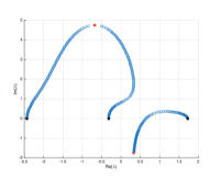
Figure 9. The first and second eigenvalues (of totally 3) collide as the parameter approaches level crossing point, giving the transposition $(12)$.

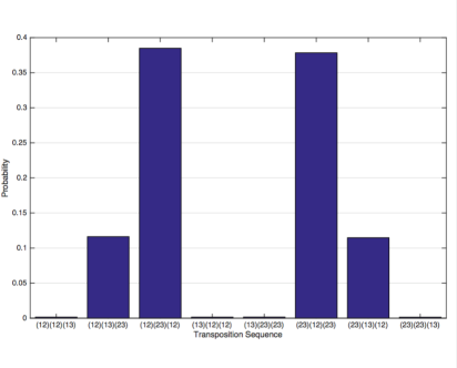
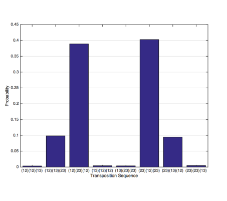
Figure 10. The probabilities of the monodromy triples of transpositions for $GUE_{3}$- and $GOE_{3}$-matrices.

Numerical experiments were carried out in MATLAB. Namely, the MATLAB-code computed the transposition associated to level crossing point $\lambda$ of a pair of matrices $(A,B)$. More exactly, the program calculated the eigenvalues of $A+(Re(\lambda)+\epsilon Im(\lambda))B$ as $\epsilon$ runs from $0$ to $1$ in steps of $0.01$. A typical plot of the eigenvalues during this process is shown in Fig. 9. At $\epsilon=0$ all of the eigenvalues are real, so we can number them in the increasing order. For each new $\epsilon$, the new eigenvalues are assigned the same numbers as the closest eigenvalues obtained for the previous value of $\epsilon$. Then, when two eigenvalues collide at $\epsilon=1$, the numbers assigned to these two colliding eigenvalues give the transposition corresponding to level crossing point $\lambda$. By following this procedure shown in Figure 9 for each of level crossing points in the upper half-plane in order of increasing real part, one obtains triples of transpositions associated to $(A,B)$. This triple of transpositions complete determines the monodromy of the linear family (1.1). Because errors can occur if the real parts of different level crossing points are very close, we discarded such pairs of matrices when gathering monodromy statistics. This procedure was carried out in case of $GUE_{3}$- and $GOE_{3}$-ensembles. The resulting statistics for $GUE_{3}$ (top) and $GOE_{3}$ (bottom) are shown in Figure 10.

Statistical results for $GE_{3}^{{\mathbb{C}}}$-ensemble.

In this case, in order to calculate the monodromy seqeunce for a general matrix family (1.1), we must first choose a base point for the system of closed paths in the $\lambda$-plane which is (generically) not a level crossing point. We choose $\lambda=0$, since typically the origin is not a level crossing point for a general pair of matrices, and the preimages of $0$ are precisely the eigenvalues of $A$. Using $\lambda=0$ as a base point, we need to order our level crossing points with respect to the origin and to choose a system of paths such that

(i) each path begins and ends at $0$;

(ii) each path goes around exactly one level crossing point;

(iii) each path does not intersect any other path except at the origin.

As already mentioned, these level crossing points are all generically simple; so as $\lambda$ traverses a path around one level crossing point and returns to the origin, exactly two of the eigenvalues of $A$ will interchange. Thus we obtain a transposition in the symmetric group $S_{n}$. To do this we have to order the preimages of our starting point (i.e., the eigenvalues of $A$) and keep track of how these preimages change as we follow each path. This procedure gives us an $n(n-1)$-tuple of transpositions in $S_{n}$. Since the concatenation of all paths encompasses all of our level crossing points, the product of all transpositions in the chosen order equals to the identity permutation. When $A$ and $B$ are independently chosen from $GE_{n}^{{\mathbb{C}}}$, the arguments of our level crossing points are uniformly distributed, so we may order our level crossing points by the argument. However the choice of which level crossing point is first and whether the level crossing points are ordered clockwise or counterclockwise is arbitrary. The paths we choose will start and end at $0$ and go around these level crossing points in a natural way. An example of how we choose such paths is shown in Fig. 11.

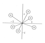
Figure 11. An example of paths in the $\lambda$-plane chosen to determine the monodromy for pairs $(A,B)$ from $GE_{3}^{{\mathbb{C}}}$.

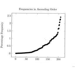
Figure 12. Frequencies of 240 possible $6$-tuples of transpositions from $S_{3}$ in the ascending order.

For $A$ and $B$ in $GE_{3}^{{\mathbb{C}}}$, there are 240 sequences of $6$-tuples of transpositions $(\sigma_{1},\sigma_{2},\dots,\sigma_{6})$ from $S_{3}$ satisfying the conditions:

(i) they generate the symmetric group $S_{3}$;

(ii) the product $\sigma_{1}\cdot\sigma_{2}\cdot\ldots\cdot\sigma_{6}$ coincides with the identity permutation $(1,2,3).$

Using a similar MATLAB-code to determine the monodromy transpositions, we generated 150000 random matrix pairs in $GE_{3}^{{\mathbb{C}}}$ and calculated their monodromy sequences. Our numerical results show the following, see Fig. 12.

(i) Of the 240 possible cases, only 209 were realized and only 204 were realized more than once.

(ii) The most common monodromy sequences were $(23)(12)(23)(12)(23)(12)$, which occurred with the frequency 2.43 % and $(12)(13)(13)(23)(23)(12)$ which occurred with the frequency 2.29 %.

(iii) Monodromy sequences in which one permutation occurs four times in a row followed by two occurrences of another permutation and their cyclic permutations (for example, $(12)(12)(12)(12)(13)(13)$ or $(12)(23)(23)(23)(23)(12))$ were the most rare, occurring only once or not at all.

Remark 8.

One particularly strange and interesting result is that the labelling of the eigenvalues seems to affect the frequencies with which certain monodromy sequences appear. In the case of $GE_{3}^{{\mathbb{C}}}$-matrices, one can relabel the three preimages of $\lambda=0$, i.e., the eigenvalues of $A$, by using the action of $S_{3}$. Usually, about half of these six group elements change the frequency by either doubling or halving the original one. The other half of the group tends to keep the frequency the same, but exactly which members of $S_{3}$ do what varies from case to case. We have not been able to find a pattern of or an explanation to why relabelling changes the frequencies in this peculiar way.

7. Final remarks

In connection with our topic, one can naturally ask why we only restrict ourselves to consideration of the distributions of a single level crossing point on $\mathbb{C}$ and are not trying to obtain information about the joint distribution of all $n(n-1)$ level crossing points which obviously exists in all the above cases. It turns out that for $n>3$, not all $n(n-1)$-tuples of complex numbers can be realized as level crossings and even the description of the loci of realizable $n(n-1)$-tuples is very complicated. This fact definitely means that at least for $n>3$, to get the joint distribution of level crossings on such loci will be a formidable (if not completely impossible) task, comp. e.g. [OnSh]. On the other hand, in the simplest case $n=2$, we calculate and use such joint distributions below.

References

- [AGZ] G. W. Anderson, A. Guionnet, O. Zeitouni, An Introduction to Random Matrices. Cambridge Studies in Advanced Mathematics, 118. Cambridge University Press, Cambridge, 2010. xiv+492 pp.
- [Chi] http://mathworld.wolfram.com/ChiDistribution.html
- [BW] C. M. Bender, T. T. Wu, Anharmonic oscillator. Phys. Rev. (2) 184 (1969), 1231–1260.
- [BDCP] O. Bohigas, J. X. De Carvalho, and M. P. Pato, Structure of trajectories of complex-matrix eigenvalues in the Hermitian–non-Hermitian transition, Phys. Review E 86, 031118 (2012).
- [CHM] P. Cejnar, S. Heinze, and M.Macek, Coulomb analogy for nonhermitian degeneracies near quantum phase transitions, Phys. Rev. Lett. 99, 100601.
- [GP] A. Galligo, A. Poteaux, Computing monodromy via continuation methods on random Riemann surfaces, Theor. Comp. Sci., 412, 16 (2011), 1492–1507.
- [Ka] T. Kato, Perturbation theory for linear operators. Reprint of the 1980 edition. Classics in Mathematics. Springer-Verlag, Berlin, 1995. xxii+619 pp.
- [MNOP] N. Michel, W. Nazarewicz, J. Okolowicz, and M. Ploszajczak, Open problems in the theory of nuclear open quantum systems, Journal of Physics G: Nuclear and Particle Physics, Volume 37, Number 6.
- [OnSh] J. Ongaro, B. Shapiro, A note on planarity stratification of Hurwitz spaces, Canadian Mathematical Bulletin vol 58, issue 3 (2015) 596–609.
- [Ro] I. Rotter, Exceptional Points and Dynamical Phase Transitions, Acta Polytechnica Vol. 50 No. 5/2010.
- [RaGaPrPu] S. R. Garcia, E. Prodan, and M. Putinar, Mathematical and physical aspects of complex symmetric operators, Journal of Physics A: Mathematical and Theoretical, vol. 47, number 35 (2014)
- [ShTaQu] B. Shapiro, M. Tater, On spectral asymptotics of quasi-exactly solvable quartic and Yablonskii-Vorob’ev polynomials, arXiv:1412.3026, submitted.
- [ShT] B. Shapiro, M. Tater, On spectral asymptotics of quasi-exactly solvable sextic, Experimental Mathematics, https://doi.org/10.1080/10586458.2017.1325792.
- [ShZa1] B. Shapiro, K. Zarembo, On level crossing in random matrix pencils. I. Random perturbation of a fixed matrix, Journal of Physics A: Mathematical and Theoretical, Volume 50(4).
- [GrShZa3] T. Grøsfjeld, B. Shapiro, K. Zarembo, Level crossing in random matrices. III. Analogs of Wigner and Girko’s laws, in preparation.
- [Sm] A. Smilga, Exceptional Points of Infinite Order Giving a Continuous Spectrum, International Journal of Theoretical Physics 2014
- [SH] W.-H. Steeb and Y. Hardy, Exceptional points, non-normal matrices, hierarchy of spin matrices and an eigenvalue problem, International Journal of Modern Physics C 2014 1450059.
- [ZVW] M. R. Zirnbauer, J. J. M. Verbaarschot, H.Ã. Weidenmüller, Destruction of order in nuclear spectra by a residual GOE interaction, Nuclear Physics A411 (1983) 161–180.