Addressing Class Imbalance in Classification Problems of Noisy Signals by using Fourier Transform Surrogates

Abstract

Randomizing the Fourier-transform (FT) phases of temporal-spatial data generates surrogates that approximate examples from the data-generating distribution. We propose such FT surrogates as a novel tool to augment and analyze training of neural networks and explore the approach in the example of sleep-stage classification. By computing FT surrogates of raw EEG, EOG, and EMG signals of under-represented sleep stages, we balanced the CAPSLPDB sleep database. We then trained and tested a convolutional neural network for sleep stage classification, and found that our surrogate-based augmentation improved the mean F1-score by 7%. As another application of FT surrogates, we formulated an approach to compute saliency maps for individual sleep epochs. The visualization is based on the response of inferred class probabilities under replacement of short data segments by partial surrogates. To quantify how well the distributions of the surrogates and the original data match, we evaluated a trained classifier on surrogates of correctly classified examples, and summarized these conditional predictions in a confusion matrix. We show how such conditional confusion matrices can qualitatively explain the performance of surrogates in class balancing. The FT-surrogate augmentation approach may improve classification on noisy signals if carefully adapted to the data distribution under analysis.

I Introduction

Classification problems in biomedical signals are often imbalanced by one or more orders of magnitude. For example, epileptic seizures are rare minute-long events that interrupt hours, days or even weeks of apparently normal cortical activity in the electroencephalogram (EEG) [1]. As another example, certain transitional sleep stages, such as S1 and S3, are underrepresented with respect to more stable stages such as wakefulness or Rapid Eye Movement (REM) sleep [2]. Rare events, such as a possibly fatal status epilepticus or sleep-onset REM indicative of narcolepsy, are especially important in the biomedical realm. It it is therefore imperative that such underrepresented classes are not swamped by the more prevalent ones.

Classification algorithms such as logistic regression, support vector machines, and random forest models can be extended to incorporate class imbalances in their cost function structure (see Haixiang et al. [3] for a review on class balancing). However by design, such extensions are aimed at general applicability, offering only little flexibility to incorporate domain specific knowledge. In mini-batch-based methods of deep learning, the imbalanced class distribution is typically equilibrated by discarding examples of prevalent classes, or repeating those in the minority. A ten-fold up-sampling may, however, lead to partial over-fitting whereas under-sampling unsatisfactorily discards vast amounts of valuable data.

Instead it has been proposed to sample from inferred distributions of minority classes [4]. In principle, deep generative models, in particular generative adversarial networks, can be used to approximate examples from these distributions [5, 6]. However, these methods are very data-hungry, and we believe they will likely fail to generate a variety of examples of rare classes in a dataset.

Class imbalance problem has also been addressed in the development of automatic sleep-staging systems (see Aboaloayon et al. [7] for a survey on such systems). However in the few deep learning approaches we found, classes were balanced by either discarding data [8, 9], or by up-sampling through repetitions of data [10]. Both approaches introduce biases in the predictions, either falsely pointing away from abnormality or falsely predicting illnesses. Possible remedies can come from domain-knowledge based models of the rare class, which can either be based in physical understanding of the biophysical process that generates the observations, or through a statistical approach.

In this article, we discuss up-sampling based on Fourier-Transform (FT) surrogates [11]. We further describe a surrogate-based method to construct saliency maps for a trained classifier. Specifically, we measure the response of inferred class probabilities under a surrogate replacement of short data segments. Our method adds to the several techniques that have been developed for image data, such as methods of gradient ascent, saliency maps [12], and deconvolution networks [13]. Previously the surrogate approach has been developed to test the hypothesis that a signal has been generated by a linear stationary stochastic process, and has been previously applied to EEG signals in this context [14]. However, we present a very different utilization in exploring the question of how surrogates can facilitate machine learning, both, in training classifiers and in analyzing what these learn to recognize.

II Methods

II-A Surrogates based on the Fourier Transform

The complex Fourier components $s_{n}$ of a signal $x_{n}$ can be decomposed into amplitudes $a_{n}$ and phases $\varphi_{n}$ as $s_{n}=a_{n}e^{i\varphi_{n}}$. Sample sequences of stationary linear random processes are uniquely defined by the Fourier amplitudes $a_{n}$, whereas their Fourier phases are random numbers in the interval $[0,2\pi)$. Under this assumption, we can draw a new sequence $y_{n}$ that is statistically independent from $x_{n}$ while representing the same generating distribution as first demonstrated by Theiler [15]. We simply replace the Fourier phases of $s_{n}$ by new random numbers from the interval $[0,2\pi)$, and apply the inverse Fourier transform.

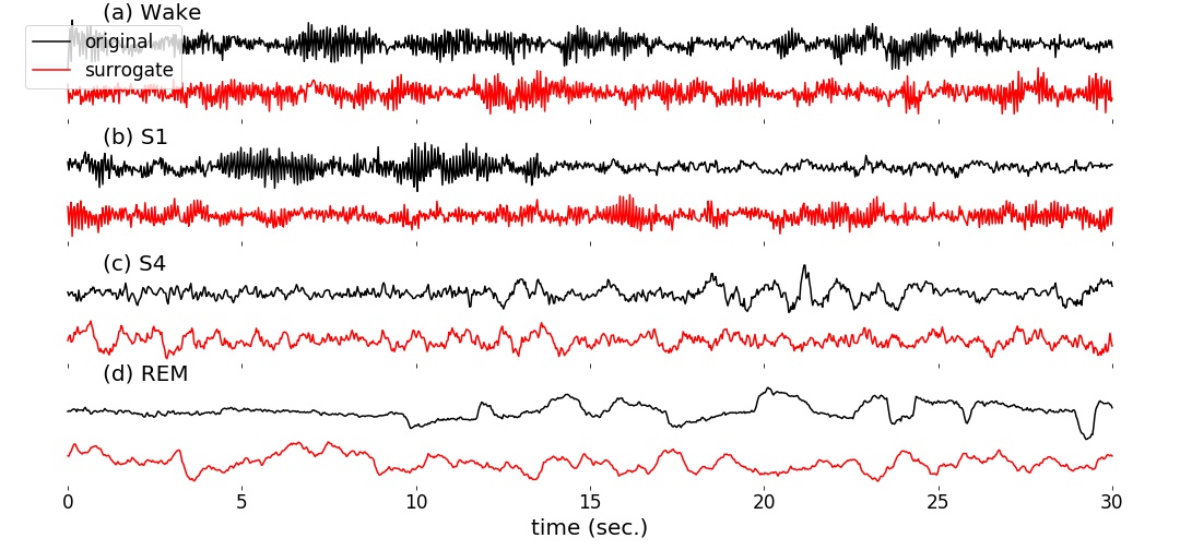
Under the assumptions of linearity and stationarity, we use this FT-surrogate method to generate new independent samples of the sleep database analyzed here. In Fig. 1, we show examples of EEG segments together with examples of their FT surrogates. Example (a) is dominated by EEG alpha waves centered around 10-Hz, wherein for example (b), such alpha waves are only visible in the segment’s first half. Comparing their surrogates allows us to understand better the effect of nonstationarity on the FT surrogate technique. While the surrogate represents the data in example (a) visually well, surrogate (b) does not show a strong localization of the alpha waves to a particular subsection. The power in this band is smeared across the whole surrogate segment thus leading to a very different visual appearance.

Figure 1: Examples of FT surrogates. We show four 30-second signals of EEG (a-c) and EOG (d) from CAPSLPDB recorded during different stages of sleep (indicated). Each signal (black line) is counterposed with a representation of its FT surrogates (red line). Panel (b) illustrates the effect of non-stationarity on the technique, Panel (d) that of nonlinearity.

Schreiber et al. [16] extended the FT-surrogate method to simultaneously model the time-domain amplitude distribution $P(x_{n})$ in addition to the Fourier-amplitude distribution $P(s_{n})$ of the original signal. In short, their algorithm starts by computing a regular FT surrogate. Next, the time-domain distribution of the surrogate is replaced by the original one. Then,the adjusted surrogate is Fourier transformed again and the Fourier distribution is replaced by the original one. The last two steps are repeated iteratively until the time-domain distribution converges sufficiently. Accordingly, these surrogates are called iterative amplitude-adjusted FT (IAAFT) surrogates.

II-B Polysomnographic Database

We processed the CAPSLPDB sleep database consisting of 101 overnight polysomnographies (PSGs) [17, 18]. Each recording contained about eight hours of multichannel recordings and sleep-stage annotations scored by an expert according to R&K 68 rules [19]. We did not take into account recordings rbd11, brux1, and nfle27 because of missing sleep scores, and n4, n8, n12, and n16 because these only contained EEG channels.

The remainder of recordings were divided into five equidistant age bins. The division was based on the data distribution.

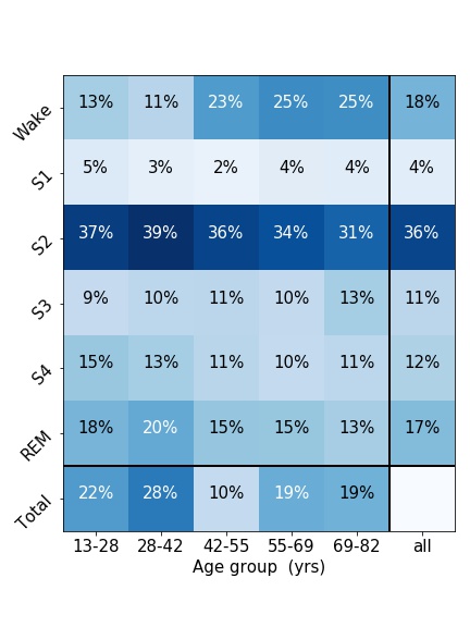
Each record had been divided in 30-second intervals each assigned one of the sleep stages Wake, S1, S2, S3, S4, REM, or MT by an expert sleep technician. In Fig. 2, we summarize the distribution of stages stratified by age groups. We ignored stage MT which occurred only $685$ times. In each age group, stage S1 was least well represented, averaging at $4\%$ across all groups. The fraction of stage Wake increased with age, and meanwhile the fraction of S4 and REM decreased.

Figure 2: Stage distribution across age groups. The relative histogram displays the distribution of all 107,738 epochs stratified by age and sleep stage.

From all available channels in each recording, we select a subset including two EEG channels, one EOG, and one EMG channel, which is a maximal subset included in all recordings. The available EEG channels were also heterogeneous regarding the recording site and derivation. They were selected with a preference list (numbers included EEG1 and EEG2): F3-C3 ($n=67$), P3-O1 ($67$), C4-M1 ($29$), F4-C4 ($26$), C3-M2 ($6$), O2-M1 ($3$), P3-Cz ($2$), F7-Cz ($2$). We resampled all signals to $32$ Hz after applying a $13$ Hz $4$-th order Butterworth low-pass filter to reduce aliasing.

Alongside different stages of sleep, aging is also known to correlate with characteristic EEG patterns. The co-variation leads to an implicit class under-representation of wakefulness in young, for example. Moreover, the database consists of individuals suffering from various diseases or disorders that are represented differentially across age, and available channels reflect to some extend the disease-specific investigation: records of young nocturnal-frontal-lobe-epilepsy patients included more EEG channels than regular PSGs, for example. We do not attempt to address all of these sources of class imbalance within the scope of this article, because on this level of detail, the present database is too small.

II-C Network Architecture and Training

We explored a convolutional neural-network architecture as a deep learning model for our sleep database. The goal was to optimize the F1-score for all six classes across the different age groups. We used Google Cloud’s ml-engine infrastructure for all computations including Bayesian hyper-parameter optimization.

Our architecture takes as input 30-second raw sequences of two EEG, one EMG, and one EOG channel as one example, and outputs soft maximum-based probabilities for the six classes Wake, S1, S2, S3, S4, and REM. Two parts constitute our network architecture: first each channel is processed by dedicated neural networks only operating on that one channel; and second, their outputs are merged to process interrelation among channels. Note, that the 4-channel input would suffice for sleep-scoring experts to deduce sleep stages. The network architecture is summarized in detail in Tab. I.

Channel pipes. In the first stage each channel is processed with a pipe of one-dimensional convolutional layers. While all pipes share the same architecture, each channel type has its own parameters, i.e. the two EEG channels share the same parameters. We choose parameter sharing across EEG channels because the heterogeneity in our dataset prohibited to train dedicated channels for specific electrode locations. Choosing the same pipe architecture for each channel facilitated joining their outputs in the second stage. After each convolutional layer we apply dropout with $p=0.33$. The Scale layer was initialized with a factor $0.05~{}\mu$V^-1. Biases were initialized as zero, and weights were initialized drawing from standard Glorot-uniform distributions [20].

Joined pipe. In the second stage, outputs of the first stage are stacked to form a $(n,4,f)$-dimensional tensor, where $f$ is the number of filters, and $n$ the length of each of the four joined sequences. A two-dimensional convolution layer is applied to the result, followed by two dense layers and the six-neuron soft-max layer to be matched with class probabilities. After the first two dense layers, we apply dropout with $p=0.015$. Biases were initialized as zero, and weights were initialized drawing from a Glorot uniform distribution.

TABLE I: Neural Network architecture. F: number of filters, W: dimension of each filter, S: Stride parameter, ReLU: Rectified linear unit.

Name	Description	Output
Channel-pipe architecture
each with 32,936 trainable parameters.
Input	30-second signal	$960$
Scale	Scalar rescaling	$960$
Conv1D	W: 16, F: 16, ReLU	$960\times 16$
MaxPool	W: 3, S: 2	$480\times 16$
Conv1D	W: 19, F: 19, ReLU	$480\times 19$
MaxPool	W: 3, S: 2	$240\times 19$
Conv1D	W: 23, F: 23, ReLU	$240\times 23$
MaxPool	W: 3, S: 2	$120\times 23$
Conv1D	W: 27 , F: 27, ReLU	$120\times 27$
MaxPool	W: 3, S: 2	$60\times 27$
Joined-pipe architecture
with 64,371 trainable parameters.
Input	Output of channel pipes	$60\times 4\times 27$
Conv2D	W: $20\times 4$, F: 10, ReLU	$41\times 1\times 10$
Dense	85 neurons, ReLU	$85$
Dense	85 neurons, ReLU	$85$
Dense	6 neurons, soft-max	$6$

We trained the network on $7000$ mini-batches of $128$ examples, and using an RMS-Prop optimization algorithm with a learning rate of $0.0016$, a decay parameter of $0.9$, and no momentum [21]. The number of steps was chosen through our experience of visually inspecting validation and training loss, and assured that these quantities always reached stable values.

II-D Validation Split and Data Sampling

We split off a validation set from the database by holding one recording back from each age group. On these five recordings, we validated an instance of a neural network which we trained on the training set consisting of all other records. In a 5-fold cross validation, we split the database (and trained networks) five times, each with different validation recordings. This yielded a total validation set of five recordings from each age group, i.e. a total of 25 recordings.

During training, we sorted the training set by stage label for up-sampling and augmentation which we controlled by two parameters $\beta\in[0,1]$ and $\alpha\in[0,1]$. As a last step, we shuffled the processed training set to randomly group examples into mini-batches of size $128$.

Up-sampling. We computed the number of repetitions $n_{c}$ of under-represented class $c$ necessary to match the number of the most frequent class. We then multiplied $n_{c}$ by a factor $\beta$, and added a corresponding number of random repetitions to the training set. The factor allowed us to control up-sampling. For the presented results, we set $\beta=0.9$.

Augmentation. Each channel in the repeated examples were replaced by FT surrogates with probability $\alpha$. That means for a given repeated example that only some of its channels could be augmented by surrogate replacements.

With this publication we provide the preprocessed database and scripts reproducing our results.

III Results

III-A Training with FT Surrogate-based Class Balancing

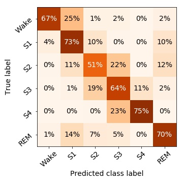
We started our analysis by training the feed-forward neural network model without replacing any repeated signals by FT surrogates ($\alpha=0$). Our training did not show considerable over-fitting as indicated by a close proximity of training- and test-set accuracies. Though not groundbreaking, our classification results on the five-fold validation set shown in Fig. 3 were within the range of previously reported results for sleep-stage classification, especially for the very complex CAPSLPDB.

Figure 3: Confusion matrix of test-set predictions. We evaluated the network on examples from the test set and computed the fraction of labels of a certain class with respect to their predictions shown in this color-coded confusion-matrix representation.

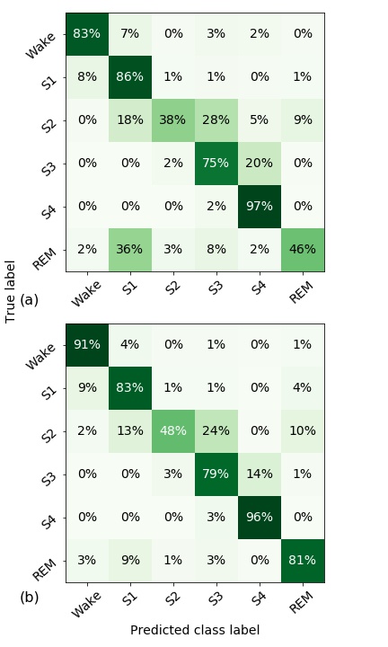
We leveraged the trained model to investigate how well signals of different sleep stages are represented by their FT surrogates. For each correctly predicted example, we computed a surrogate and re-applied the classifier. We analyzed the confusion matrix for these surrogate labels conditioned on a correct original prediction. As shown in Fig. 4(a), FT surrogates of stages Wake, S1, and S4 were predicted to be from the correct class with probabilities larger than 80%, whereas surrogates of S2 and REM showed lowest conditional accuracies. Comparing the off-diagonal matrix elements, we found that S1-surrogates are more often miss-classified as Wake, S2 as S3, S3 as S4, and REM as S1. Exemplary, the miss-classification S1$\to$Wake may be explained by the redistribution of non-stationary bursts of alpha oscillations when drawing a surrogate as visible in Fig. 1(b): in the surrogate, the alpha rhythm appears in more than 50% of the segment thus making a classification Wake more likely by eye and by algorithm. We hypothesize that miss-classifications S2$\to$S3, S3$\to$S4, and REM$\to$S1 are also due to non-stationarities, i.e., K-complexes, and bursts of delta waves or rapid eye movements. We also evaluated the conditional confusion matrix when replacing the original correctly predicted examples with IAAFT surrogates, as shown in Fig. 4(b). Comparing the conditional accuracies of FT and IAAFT surrogates, we observed that the latter were equal or better predicted for all stages except S1. Standard deviations in conditional confusion values were around 1%.

Figure 4: Conditional confusion matrix. The correct predictions (diagonal in Fig. 3) were transformed to (a) FT surrogates, and (b) IAAFT surrogates, and than re-scored by the sleep-staging algorithm. The result is presented in respective conditional confusion matrices.

Next, we increased the augmentation probability $\alpha$ to values between $0$ and $1$, thus replacing fractions of up-sampled signals by FT surrogates. At each $\alpha$, we performed our scheme of five-fold cross-validation and observed how prediction probabilities changed. We found a consistent maximum of the F1-score at about $\alpha=0.4$ (cf. Fig. 5).

Figure 5: Average F1-score versus augmentation probability. The average F1-score depending on surrogate augmentation probability $\alpha$ shows a distinct maximum, both for the test set as well as for the training set.

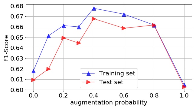
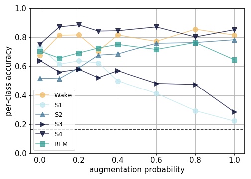
The convex dependence of the F1-score on $\alpha$ can be better understood when decomposing the measure into its constituent per-class accuracies summarized in Fig. 6. While the accuracy of stages Wake, S2, and S4 slightly increase, the S1- and S3-accuracies rapidly decrease towards zero beyond $\alpha>0.4$. These two opposing objectives create the quantitative compromise exhibited as a non-trivial maximum in the $\alpha$-dependence of the F1-score. Notice that the accuracy of stage S2 showed the greatest benefit of surrogate-based up-sampling, of which no surrogates were created.

Figure 6: Per-class accuracy versus augmentation probability. The per-class accuracy depending on surrogate augmentation probability $\alpha$ shows slightly increasing patterns for stages Wake, S2, S4, and REM, and sharply decreasing patterns for stages S1, and S3. This discrepancy explains to a certain extend the convex F1-score dependence (cf. Fig. 5).

Unfortunately, we were not yet able to evaluate and compare IAAFT surrogates with these results due to temporal and budget constraints.

III-B Partial FT Surrogates to Analyze Class Probabilities

Based on FT surrogates we propose a novel technique to create saliency maps from which we can read out the relative importance of a subsection of a signal for the predicted class probabilities. First, we selected a window length and a subset of channels in which we presumed to find a relevant feature. To query the relevance of the data at a given location in the epoch, one could, naively, zero-out the subsection in question and observe how inferred probabilities change. However, imputing such quiescent periods can introduce class biases; for example a very low-voltage EMG signal strongly indicates REM sleep over other sleep stages. Instead, we spliced out the signal window, and replaced the subsection with an FT surrogate generated from the remainder of the signal under analysis as visualized in Fig. 7. All splicing was performed smoothly by cosine half-wave interpolation of $0.5$-second overlaps.

Figure 7: Example of a partial FT surrogate. A 4-second subsection of an EEG signal recorded during stage Wake is shown (black line), together with a partial FT surrogate (red line). The partial surrogate replaced the anomaly in the segment between second 13 and 17. Note that the surrogate dominantly contains the $\sim$ 10-Hz alpha waves also visible in the rest of the signal.

Figure 8: Partial FT surrogate analysis. This 30-second REM epoch was miss-classified as S2 with $P(\tt{S2})=68\%$ (black dashed line). The suspicion was that the K-complex at about 17 seconds caused the miss-classification. The used classifier was trained with $\alpha=0.4$. (a) We analyzed the epoch with the partial FT-surrogate technique to both EEG signals using a 5-second-long moving window with an overlap of $0.5$ seconds, and $500$ surrogate replacements. The averaged probability of S2 and REM change as a function of the window location. The temporary reversal of probabilities indicates that the K-complex at about 17 seconds caused the miss-classification. (b) The surrogate approach is counterposed with simple zeroing out, in which an equivalent 5-second window is (smoothly) replaced by zeros. This naive approach also shows a reversal of probabilities, but at the wrong position. Note that there was no offset in the signal.

For a given window location, the partial surrogate replacement was performed multiple times. For each replacement, the epoch was then processed by our sleep-staging algorithm and the class probabilities were recorded. Finally, we averaged these class probabilities over the independent replacements. The averaged probabilities as a function of the window position yielded a saliency map that described the relevance of localized features for the classification result found in for a specific example.

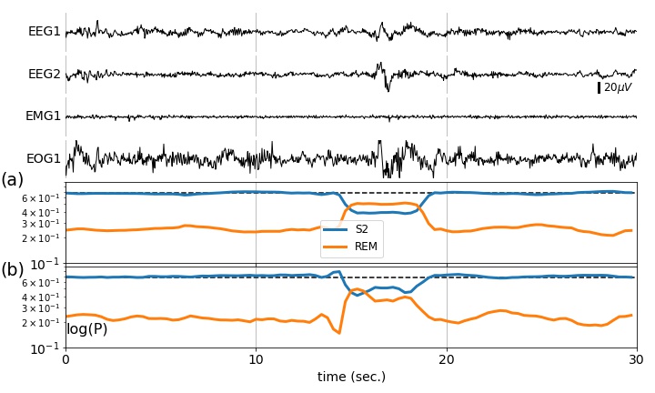
We demonstrate the partial FT surrogate technique with an example epoch of stage REM that has been misclassified as stage S2 by our algorithm (cf. Fig. 8). In the latter half of the example, there is a K-complex visible in both EEG-channels and the EOG-channel, which according to the rules leads to a stage change to S2 in the following epoch. Had it occurred in the earlier half of the example, the example would have been scored as S2.

We analyzed this epoch using our partial-surrogate method (cf. Fig. 8(a)), and counterposed the result with naive zeroing out of equivalent subsections (cf. Fig. 8(b)). The prediction probabilities of sleep states S2 and REM crossed or reversed as the surrogate replacement 5-second window slides across the location of the K-complex. The probabilities also reversed for the zero-out method, however, not concurrently with the visually identified event.

IV Discussion

We explored two applications of Fourier transform (FT) surrogates to sleep stage classification: we analyzed how up-sampling minority examples with FT surrogates affects the prediction scores. Furthermore, we described a method of saliency maps based on partial FT surrogates that allow us to analyze how individual class probabilities depend on subsections of the signals.

The convex dependence of the F1-score on the augmentation probability indicates a possible benefit of surrogate-based up-sampling. However, this might not be the case for all class labels equally. Increases in the S2-accuracy seemed to be at the expense of stages S1 and S3 for larger values of $\alpha$. Based on these results, we hypothesize that the effect of surrogate augmentation on an individual class accuracy does not directly depend on their conditional prediction accuracies, which are on the diagonal of the conditional confusion matrix (cf. Fig. 4(a)); instead, augmentation may introduce mixing between class labels indicated by a large off-diagonal element upon which the accuracy of one of the mixed labels will dominate. Accordingly, we hypothesize the accuracy increase of S2 and REM to be at the expense of classification accuracy of S1, and the increase in accuracy for S2 and S4 at the expense of classification accuracy of S3. The conditional confusion matrix of IAAFT surrogates exhibit higher accuracy and lower off-diagonal elements indicating mixing of labels (cf. Fig. 4(b)). One interpretation of the results is that IAAFT surrogates are able to model the data distribution more accurately; on the other hand, the results are also consistent with the data distribution to be highly collapsed into regions that are well predicted by our algorithm. While the former would suggest benefits of using IAAFT over simple surrogates, the latter would mean that using IAAFT would increase the tendency to over-fit the data. To date, we understand little about the topological properties of the IAAFT distribution and therefore it is hard to reason which effect will dominate. Therefore, it would be interesting to see how training with IAAFT surrogates impacts accuracy scores in this and other examples of biomedical data analysis. Specifically we predict from our hypothesis, that augmentation with IAAFT surrogates will have a less negative impact on the S1 classification accuracy.

Partial surrogate analysis is not restricted to neural-network based or other differentiable classifiers as these saliency maps are created purely by controlling input and output probabilities. Also, the technique, aimed at transient signal features, does not greatly suffer from the requirement of stationarity since the replaced subsections are of lengths at which EEG signals are approximately statistically stationary. However, features without temporal localization cannot be delineated with our technique. For example, a constant alpha-wave background will not be detected to distinguish Wake from S1 because the surrogate replacement will also contain alpha waves (compare Fig. 1(a) and (b)). Such features are more likely to be highlighted by gradient-based saliency maps, and when training on a wavelet representation of the signal as data input. The example shown in Fig. 8 highlights the strength of our technique, where it allowed us to gather evidence that our sleep-staging algorithm learned about the existence of K-complexes and their relevance of distinguishing between REM and S2 (cf. Fig. 8). This was particularly unclear given the relatively poor accuracy of the classifier.

We conclude from the present work that the ability to draw independent examples from the data distribution is important in training, analysis, and validation of deep machine-learning models. As in this work, such examples can be used to balance and augment a database to achieve better generalization, and to understand which statistical properties of data are instrumental to black-box learning algorithms to make predictions. Unless the database is large enough to train a deep generative model that mimics the data distribution, it is necessary to build the generator from a strong set of constraints rooted in specific domain knowledge. This is especially the case for under-represented classes for which we do not have a lot of data. Usage of FT surrogates is constrained to stationary linear random data as the current work illustrates. For IAAFT surrogates we cannot formulate the precise constraints. In the future, it may also be helpful to query mechanism-based models to generate surrogates in situations, particularly for nonlinear signals, that are not well represented by FT-based surrogates, such as electrocardiograms.

In the future, we plan to adopt our approach to identify ambiguous or mislabeled data which are often mislabeled for two general reasons: natural inter- and intra-observer variability for transitional epochs, and errors due to quantization or coarse windowing of data. Although the issue of only moderate inter- and intra-rater agreement levels is a known issue in sleep stage labeling [22], the latter issue is a particularly under-explored problem in sleep stage classification. In particular we plan to use partial FT surrogate analysis to identify epochs ambiguous due to short transient events. The ability to programatically exclude such edge cases from a training may enhance the efficacy of sleep-stage classification.

References

- [1] F. Mormann, R. G. Andrzejak, C. E. Elger, and K. Lehnertz, “Seizure prediction: The long and winding road,” Brain, vol. 130, no. 2, pp. 314–333, 2006. [Online]. Available: http://dx.doi.org/doi:10.1093/brain/awl241
- [2] M. A. Carskadon and W. C. Dement, “Normal human sleep: An overview,” Principles and Practice of Sleep Medicine, vol. 4, pp. 13–23, 2005.
- [3] G. Haixiang, L. Yijing, J. Shang, G. Mingyun, H. Yuanyue, and G. Bing, “Learning from class-imbalanced data: Review of methods and applications,” Expert Sys. Appl., vol. 73, pp. 220–239, 2017. [Online]. Available: http://dx.doi.org/10.1016/j.eswa.2016.12.035
- [4] N. V. Chawla, K. W. Bowyer, L. O. Hall, and W. P. Kegelmeyer, “SMOTE: Synthetic minority over-sampling technique,” J. Artif. Intell. Res., vol. 16, pp. 321–357, 2002. [Online]. Available: http://dx.doi.org/10.1613/jair.953
- [5] M. Mirza and S. Osindero, “Conditional generative adversarial nets,” arXiv preprint arXiv:1411.1784, 2014.
- [6] A. Antoniou, A. Storkey, and H. Edwards, “Data augmentation generative adversarial networks,” arXiv preprint arXiv:1711.04340, 2017. [Online]. Available: http://arxiv.org/abs/1711.04340
- [7] K. A. Aboalayon, M. Faezipour, W. S. Almuhammadi, and S. Moslehpour, “Sleep stage classification using eeg signal analysis: A comprehensive survey and new investigation,” Entropy, vol. 18, no. 9, p. 272, 2016. [Online]. Available: http://dx.doi.org/10.3390/e18090272
- [8] O. Tsinalis, P. M. Matthews, Y. Guo, and S. Zafeiriou, “Automatic sleep stage scoring with Single-Channel EEG using convolutional neural networks,” arXiv preprint arXiv:1610.01683, 2016. [Online]. Available: http://arxiv.org/abs/1610.01683
- [9] H. Dong, A. Supratak, W. Pan, C. Wu, P. M. Matthews, and Y. Guo, “Mixed neural network approach for temporal sleep stage classification,” IEEE T. Neur. Sys. Reh., no. 99, p. 1, 2017. [Online]. Available: http://dx.doi.org/10.1109/tnsre.2017.2733220
- [10] A. Supratak, H. Dong, C. Wu, and Y. Guo, “Deepsleepnet: A model for automatic sleep stage scoring based on raw single-channel eeg,” IEEE T. Neur. Syst. Reh., vol. 25, no. 11, pp. 1998–2008, Aug. 2017. [Online]. Available: http://dx.doi.org/10.1109/tnsre.2017.2721116
- [11] T. Schreiber and A. Schmitz, “Surrogate time series,” Physica D, vol. 142, no. 3, pp. 346–382, 2000. [Online]. Available: http://dx.doi.org/doi:10.1016/S0167-2789(00)00043-9
- [12] K. Simonyan, A. Vedaldi, and A. Zisserman, “Deep inside convolutional networks: Visualising image classification models and saliency maps,” arXiv preprint arXiv:1312.6034, 2013.
- [13] M. D. Zeiler and R. Fergus, “Visualizing and understanding convolutional networks,” in European conference on computer vision. Springer, 2014, pp. 818–833.
- [14] R. G. Andrzejak, K. Lehnertz, F. Mormann, C. Rieke, P. David, and C. E. Elger, “Indications of nonlinear deterministic and finite-dimensional structures in time series of brain electrical activity: Dependence on recording region and brain state,” Phys. Rev. E, vol. 64, no. 6, p. 061907, 2001. [Online]. Available: http://dx.doi.org/10.1103/PhysRevE.64.061907
- [15] J. Theiler, S. Eubank, A. Longtin, B. Galdrikian, and J. D. Farmer, “Testing for nonlinearity in time series: The method of surrogate data,” Physica D, vol. 58, no. 1-4, pp. 77–94, 1992. [Online]. Available: http://dx.doi.org/10.1016/0167-2789(92)90102-S
- [16] T. Schreiber and A. Schmitz, “Improved surrogate data for nonlinearity tests,” Phys. Rev. Lett., vol. 77, no. 4, pp. 635–638, 1996. [Online]. Available: http://dx.doi.org/10.1103/PhysRevLett.77.635
- [17] A. L. Goldberger, L. A. N. Amaral, L. Glass, J. M. Hausdorff, P. C. Ivanov, R. G. Mark, J. E. Mietus, G. B. Moody, C.-K. Peng, and H. E. Stanley, “Physiobank, physiotoolkit, and physionet,” Circulation, vol. 101, no. 23, pp. e215–e220, 2000. [Online]. Available: http://dx.doi.org/doi:10.1161/01.CIR.101.23.e215
- [18] M. G. Terzano, L. Parrino, A. Smerieri, R. Chervin, S. Chokroverty, C. Guilleminault, M. Hirshkowitz, M. Mahowald, H. Moldofsky, A. Rosa, R. Thomas, and A. Walters, “Atlas, rules, and recording techniques for the scoring of cyclic alternating pattern (CAP) in human sleep.” Sleep Med., vol. 3, no. 2, pp. 187–199, 2002. [Online]. Available: http://dx.doi.org/10.1016/S1389-9457(02)00003-5
- [19] A. Rechtschaffen and A. Kales, A Manual of Standardized Terminology, Techniques, and Scoring Systems for Sleep Stages of Human Subjects. Brain Information/Brain Research Institute, 1968.
- [20] X. Glorot and Y. Bengio, “Understanding the difficulty of training deep feedforward neural networks,” in Proceedings of the Thirteenth International Conference on Artificial Intelligence and Statistics, 2010, pp. 249–256.
- [21] T. Tieleman and G. Hinton, “Lecture 6.5 - RmsProp: Divide the gradient by a running average of its recent magnitude,” COURSERA: Neural Networks for Machine Learning, 2012.
- [22] H. Danker-Hopfe, P. Anderer, J. Zeitlhofer, M. Boeck, H. Dorn, G. Gruber, E. Heller, E. Loretz, D. Moser, S. Parapatics, B. Saletu, A. Schmidt, and G. Dorffner, “Interrater reliability for sleep scoring according to the Rechtschaffen & Kales and the new AASM standard,” J. Sleep Res., vol. 18, no. 1, pp. 74–84, 2009. [Online]. Available: http://www.ncbi.nlm.nih.gov/pubmed/19250176 http://doi.wiley.com/10.1111/j.1365-2869.2008.00700.x