Matrix Completion and Performance Guarantees for Single Individual Haplotyping

Abstract

Single individual haplotyping is an NP-hard problem that emerges when attempting to reconstruct an organism’s inherited genetic variations using data typically generated by high-throughput DNA sequencing platforms. Genomes of diploid organisms, including humans, are organized into homologous pairs of chromosomes that differ from each other in a relatively small number of variant positions. Haplotypes are ordered sequences of the nucleotides in the variant positions of the chromosomes in a homologous pair; for diploids, haplotypes associated with a pair of chromosomes may be conveniently represented by means of complementary binary sequences. In this paper, we consider a binary matrix factorization formulation of the single individual haplotyping problem and efficiently solve it by means of alternating minimization. We analyze the convergence properties of the alternating minimization algorithm and establish theoretical bounds for the achievable haplotype reconstruction error. The proposed technique is shown to outperform existing methods when applied to synthetic as well as real-world Fosmid-based HapMap NA12878 datasets.

I Introduction

DNA of diploid organisms, including humans, is organized into pairs of homologous chromosomes. The two chromosomes in a pair differ from each other due to point mutations, i.e., they contain so-called single nucleotide polymorphisms (SNPs) in a fraction of locations. SNPs are relatively rare; for humans, the SNP rate between two homologous chromosomes is roughly $1$ in $300$ base-pairs [1]. The ordered sequence of SNPs located on a chromosome in a homologous pair is referred to as a haplotype. Haplotype information is of critical importance for personalized medical applications, including the discovery of an individual’s susceptibility to diseases [2], whole genome association studies [3], gene detection under positive selection and discovery of recombination patterns [4]. High-throughput DNA sequencing platforms rely on so-called shotgun sequencing strategy to randomly oversample the pairs of chromosomes and generate a library of overlapping paired-end reads (fragments). Parts of the reads that do not cover variant positions are typically discarded; the remaining data is conveniently organized in a read-fragment matrix where the rows correspond to reads and columns correspond to SNPs. Since the SNPs are relatively rare and reads are relatively short, the read-fragment matrix is typically very sparse. If the reads were free of sequencing errors, haplotype assembly would be straightforward and would require partitioning the reads into two clusters, one for each chromosome in a pair. However, presence of sequencing errors (of the order $10^{-3}$ to $10^{-2}$) gives rise to ambiguities about the origin of reads and renders the single individual haplotyping (SIH) problem computationally very challenging.

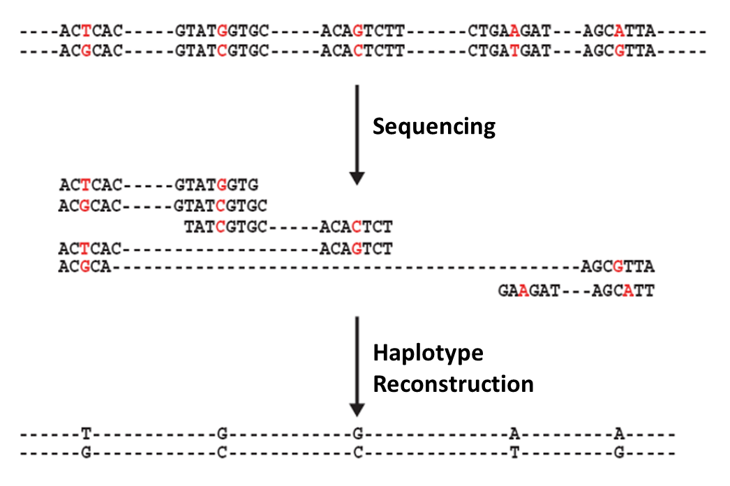
Figure 1: An illustration of the single individual haplotyping problem (often also referred to as haplotype assembly). The nucleotides marked in red denote the SNPs on a pair of chromosomes. During sequencing, paired-end reads (i.e., DNA fragments) containing the SNPs are generated from multiple copies of the chromosomal sequences; one can think of each read as being obtained by sampling (with replacement) one of the chromosomes. We assume that the relative ordering of reads can be determined by mapping them to a reference genome. The goal of single individual haplotyping is to determine the order of SNPs associated with each chromosome in the pair.

Approaches to SIH attempt to perform optimization of various criteria including minimum fragment removal, minimum SNP removal and most widely used minimum error correction (MEC) objectives [5]. Finding the optimal MEC solution to the SIH problem is known to be NP-hard [5, 6]. A branch-and-bound approach in [7] solves the problem optimally but the complexity of the scheme grows exponentially with the haplotype length. Similar approach was adopted in [8] where statistical information about sequencing errors was exploited to solve the MEC problem using sphere decoding. However, the complexity of this scheme grows exponentially with haplotype length and quickly becomes prohibitive. Suboptimal yet efficient methods for SIH include greedy approach [9], max-cut based solution [10], Bayesian methods based on MCMC [11], greedy cut based [12] and flow-graph based approaches [13]. More recent heuristic haplotype assembly approaches include a convex optimization program for minimizing the MEC score [14], a communication-theoretic approach solved using belief propagation [15], dynamic programming based approach using graphical models [16] and probabilistic mixture model based approach [17]. Generally, these heuristic methods come without performance guarantees.

Motivated by the recent developments in the research on matrix completion (overviewed in Section II-A), in this paper we formulate SIH as a rank-one matrix completion problem and propose a binary-constrained variant of alternating minimization algorithm to solve it. We analyze the performance and convergence properties of the proposed algorithm, and provide theoretical guarantees for haplotype reconstruction expressed in the form of an upper bound on the MEC score. Furthermore, we determine the sample complexity (essentially, sequencing coverage) that is sufficient for the algorithm to converge. Experiments performed on both synthetic and HapMap sample NA12878 datasets demonstrate the superiority of the proposed framework over competing methods. Note that a matrix factorization framework was previously leveraged to solve SIH via gradient descent in [18]; however, [18] does not provide theoretical performance guarantees that are established for the alternating minimization algorithm proposed in the current manuscript. An early preliminary version of our work was presented in [19].

I-A Notation

Matrices are represented by uppercase bold letters and vectors by lowercase bold letters. For a matrix ${\bf M}$, ${\bf M}^{(i)}$ and ${\bf M}_{i}$ represent its $i^{th}$ row and $i^{th}$ column, respectively. $M_{ij}$ denotes the $(i,j)^{th}$ entry of matrix ${\bf M}$ and $u_{i}$ denotes the $i^{th}$ entry of vector ${\bf u}$. ${\bf M}^{\dagger},\|{\bf M}\|_{2}$, $\|{\bf M}\|_{F}$ and $\|{\bf M}\|_{1}$ represent respectively the transpose, the spectral norm (or 2-norm), the Frobenius norm and entry-wise $\ell_{1}$ norm (i.e., $\sum_{ij}|M_{ij}|$) of the matrix ${\bf M}$, whereas the 2-norm of a vector ${\bf u}\in\mathbb{R}^{m}$ is denoted by $\|{\bf u}\|_{2}=\left(\sum_{i=1}^{m}|u_{i}|^{2}\right)^{1/2}$. Each vector is assumed to be a column vector unless otherwise specified. A range of integers from $1$ to $m$ is denoted by $[m]=\{1,2,\ldots,m\}$. $\mathbb{I}$ stands for the identity matrix of an appropriate dimension. Sign of an entry $u_{i}$ is $\text{sign}(u_{i})=1$ if $u_{i}\geq 0$, $-1$ otherwise, and $\text{sign}({\bf u})$ is the vector of entry-wise signs of ${\bf u}$. A standard basis vector with $1$ in the $i^{th}$ entry and $0$ everywhere else is denoted by ${\bf e}_{i}$. The singular value decomposition (SVD) of a matrix ${\bf M}\in\mathbb{R}^{m\times n}$ of rank $k$ is given by ${\bf M}={\bf U}\Sigma{\bf V}^{T}$, where ${\bf U}\in\mathbb{R}^{m\times k}$ and ${\bf V}\in\mathbb{R}^{n\times k}$ are matrices of the left and right singular vectors, respectively, of ${\bf M}$, with ${\bf U}^{T}{\bf U}=\mathbb{I}$ and ${\bf V}^{T}{\bf V}=\mathbb{I}$, and $\Sigma\in\mathbb{R}^{k\times k}$ is a diagonal matrix whose entries are $\{\sigma_{1},\sigma_{2},\ldots,\sigma_{k}\}$, where $\sigma_{1}\geq\sigma_{2}\geq\cdots\geq\sigma_{k}\geq 0$ are the singular values of ${\bf M}$. Projection of a matrix ${\bf M}$ on the subspace spanned by the columns of another matrix ${\bf U}$ is denoted by $\mathbb{P}_{{\bf U}}({\bf M})=\|{\bf U}{\bf U}^{T}{\bf M}\|_{2}$ and the projection to the orthogonal subspace is denoted by $\mathbb{P}_{{\bf U}^{\perp}}({\bf M})=\|(\mathbb{I}-{\bf U}{\bf U}^{T}){\bf M}\|_{2}$. Subspace spanned by vectors ${\bf u}_{i}$ is denoted by span$\{{\bf u}_{i}\}$. Lastly, ${\bf 1}_{\mathcal{A}}$ denotes the indicator function for the event $\mathcal{A}$, i.e.,${\bf 1}_{\mathcal{A}}$ = 1, if $\mathcal{A}$ is true, 0 otherwise.

II Matrix Completion Formulation of Single Individual Haplotyping

II-A Brief background on matrix completion

Matrix completion is concerned with finding a low rank approximation to a partially observed matrix, and has been an active area of research in recent years. Finding a rank-$k$ approximation ${\bf M}\in\mathbb{R}^{m\times n}$, $k<\min\{m,n\}$, to a partially observed matrix is often reduced to the search for factors ${\bf U}\in\mathbb{R}^{m\times k}$ and ${\bf V}\in\mathbb{R}^{n\times k}$ such that ${\bf M}={\bf U}{\bf V}^{T}$ [20, 21, 22, 23, 24, 25]. Formally, the low rank matrix completion problem for ${\bf M}$ with noisy entries over a partial set $\Omega\in[m]\times[n]$ is stated as

$$(\hat{{\bf U}},\hat{{\bf V}})~{}=~{}\underset{{\bf U}\in\mathbb{R}^{m\times k}\atop{\bf V}\in\mathbb{R}^{n\times k}}{\arg\min}~{}\sum\limits_{(i,j)\in\Omega}~{}({\bf R}_{ij}-{\bf U}^{(i)}{\bf V}_{j})^{2},$$ (1)

where ${\bf R}$ is the partially observed noisy version of ${\bf M}$. The task of inferring missing entries of ${\bf M}$ by the above factorization is generally ill-posed unless additional assumptions are made about the structure of ${\bf M}$ [22], e.g., ${\bf M}$ satisfies the incoherence property (see definition (II.1)) and the entries of $\Omega$ are sampled uniformly at random.

Definition II.1.

[22] A rank-$k$ matrix ${\bf M}\in\mathbb{R}^{m\times n}$ with SVD given by ${\bf M}={\bf U}\Sigma{\bf V}^{T}$ is said to be incoherent with parameter $\mu$ if

$$\|\mathbb{P}_{{\bf U}}({\bf e}_{i})\|_{2}\leq\frac{\mu\sqrt{k}}{\sqrt{m}}~{}\forall~{}i\in[m],~{}~{}\text{and}~{}~{}$$

$$\|\mathbb{P}_{{\bf V}}({\bf e}_{j})\|_{2}\leq\frac{\mu\sqrt{k}}{\sqrt{n}}~{}\forall~{}j\in[n].$$

The optimization in (1) is NP-hard [26]; a commonly used heuristic for approximately solving (1) is the alternating minimization approach that keeps one of ${\bf U}$ and ${\bf V}$ fixed and optimizes over the other factor, and then switches and repeats the process [24, 27, 28]. Each of the alternating optimization steps is convex and can be solved efficiently. One of the few works that provide a theoretical understanding of the convergence properties of alternating minimization based matrix completion methods is [24], where it was shown that for a sufficiently large sampling probability of $\Omega$, the reconstruction error can be minimized to an arbitrary accuracy. The original noiseless analysis was later extended to a noisy case in [27].

In a host of applications, factors ${\bf U}$, ${\bf V}$ or both may exhibit structural properties such as sparsity, non-negativity or discreteness. Such applications include blind source separation [29], gene network inference [30], and clustering with overlapping clusters [31], to name a few. In this work, we consider the rank-one decomposition of a binary matrix ${\bf M}\in\{1,-1\}^{m\times n}$ from its partial observations that are perturbed by bit-flipping noise. This formulation belongs to a broader category of non-negative matrix factorization [21] or, more specifically, binary matrix factorization [32, 33, 34, 35]. Related prior works include [32, 33], which consider decomposition of a binary matrix ${\bf M}$ in terms of non-binary ${\bf U}$ and ${\bf V}$, while [34] explores a Bayesian approach to factorizing matrices having binary components. The approach in [35] constrains ${\bf M}$, ${\bf U}$ and ${\bf V}$ to all be binary; however, it requires a fully observed input matrix ${\bf M}$. On the other hand, [36] considers a factorization of a non-binary ${\bf M}$ into a binary and a non-binary factor, with the latter having “soft” clustering constraints imposed. As opposed to these works, we aim for approximate factorization in the scenario where all of ${\bf M}$, ${\bf U}$ and ${\bf V}$ are binary, having only limited and noisy access to the entries of ${\bf M}$.

Next, we define the notion of distance between two vectors, which will be used throughout the rest of this paper.

Definition II.2.

[37] Given two vectors $\tilde{{\bf u}}\in\mathbb{R}^{m}$ and $\tilde{{\bf w}}\in\mathbb{R}^{m}$, the principal angle distance between $\tilde{{\bf u}}$ and $\tilde{{\bf w}}$ is defined as

$$\text{dist}(\tilde{{\bf u}},\tilde{{\bf w}})=\|\mathbb{P}_{{{\bf u}}^{\perp}}({\bf w})\|_{2}=\|(\mathbb{I}-{\bf u}{\bf u}^{T}){\bf w}\|_{2}=\sqrt{1-(\langle{\bf u},{\bf w}\rangle)^{2}},$$

where ${\bf u}$ and ${\bf w}$ are normalized forms of $\tilde{{\bf u}}$ and $\tilde{{\bf w}}$.

II-B System model

Let the number of reads carrying information about the haplotypes (after discarding reads which cover no more than one SNP) be $n$. If $m$ denotes the haplotype length ($m\leq n$), then the reads can be organized into an $m\times n$ SNP fragment matrix ${\bf R}$, whose $i^{th}$ column ${\bf R}_{i}$ contains information carried by the $i^{th}$ read and whose $j^{th}$ row ${\bf R}^{(j)}$ contains information about the $j^{th}$ SNP position on the chromosomes in a pair. Since diploid organisms typically have bi-allelic chromosomes (i.e., only $2$ possible nucleotides at each SNP position), binary labels $+1$ or $-1$ can be ascribed to the informative entries of ${\bf R}$, where the mapping between nucleotides and the binary labels follows arbitrary convention. Let $\Omega$ be the set of entries of ${\bf R}$ that carry information about the SNPs; note that the number of informative entries in each column of ${\bf R}$ in much smaller than $m$, reflecting the fact that the reads are much shorter than chromosomes. Let us define the sample probability as $p=\frac{|\Omega|}{mn}$. Furthermore, let us define the operator $P_{\Omega}:\mathbb{R}^{m\times n}\rightarrow\mathbb{R}^{m\times n}$ as

$$[P_{\Omega}({\bf R})]_{ij} =\begin{cases}R_{ij},&(i,j)\in\Omega\\ 0,&\text{otherwise}.\end{cases}$$ (2)

$R_{ij}$ represents the information about the $i^{th}$ SNP site provided by the $j^{th}$ read. Adopting the convention that $0$’s in column $j$ correspond to SNP positions not covered by the $j^{th}$ read, $P_{\Omega}({\bf R})$ becomes a matrix with entries in $\{-1,0,1\}$. Let $\mathcal{H}=\{h_{1},h_{-1}\}$ be the set of haplotype sequences of the diploid organism under consideration, with $h_{k}\in\{-1,1\}^{m},k=1,-1$. Note that the binary encoding of SNPs along the haplotypes implies that the haplotypes are binary complements of each other, i.e., $h_{1}=-h_{-1}$.

$P_{\Omega}({\bf R})$ can be thought of as obtained by sampling, with errors, a rank one matrix ${\bf M}$ with entries from $\{1,-1\}$, given by

$${\bf M}=\hat{{\bf u}}^{\star}(\hat{{\bf v}}^{\star})^{\dagger}=\sigma^{\star}{\bf u}^{\star}({\bf v}^{\star})^{\dagger}$$ (3)

where $\hat{{\bf u}}^{\star}$ and $\hat{{\bf v}}^{\star}$ are vectors of lengths $m$ and $n$ respectively, with entries from $\{1,-1\}$, ${\bf u}^{\star}$ and ${\bf v}^{\star}$ are normalized versions of $\hat{{\bf u}}^{\star}$ and $\hat{{\bf v}}^{\star}$, and $\sigma^{\star}>0$ is the singular value of ${\bf M}$. $\hat{{\bf u}}^{\star}$ represents the haplotype $h_{1}$ or $h_{-1}$ (the choice can be arbitrary) and $\hat{v}_{j}^{\star}$ denotes the membership of $j^{th}$ read, i.e., $\hat{v}_{j}^{\star}=k$ if and only if the $j^{th}$ read is sampled from $h_{k},k=1,-1$. If ${\bf N}$ denotes the sequencing error noise matrix, then the erroneous SNP fragment matrix is given by

$${\bf R} ={\bf M}+{\bf N},~{}~{}\text{or}$$

$$P_{\Omega}({\bf R}) =P_{\Omega}({\bf M})+P_{\Omega}({\bf N}).$$ (4)

The objective of SIH is to infer $\hat{{\bf u}}^{\star}$ (and $\hat{{\bf v}}^{\star}$) from the data matrix $P_{\Omega}({\bf R})$ which is both sparse as well as noisy.

II-C Noise model

Let $p_{e}$ denote the sequencing error probability. The noise matrix ${\bf N}$ capturing the sequencing errors can be modeled as an $m\times n$ matrix with entries in $\{-N_{\max},0,N_{\max}\}$, where each entry is given by

$$N_{ij} =\begin{cases}0,~{}~{}\text{w. p.}~{}(1-p_{e})\\ -2M_{ij},~{}~{}\text{w. p.}~{}p_{e}.\\ \end{cases}$$ (5)

${\bf N}$ has full rank since the errors occur independently across the reads and SNPs. The SVD of ${\bf N}$ is given by ${\bf N}={\bf U}_{N}\Sigma_{N}({\bf V}_{N})^{\dagger}$, where ${\bf U}_{N}\in\mathbb{R}^{m\times m},{\bf V}_{N}\in\mathbb{R}^{n\times m},\Sigma_{N}=\text{diag}(\sigma_{1}^{N},\sigma_{2}^{N},\ldots,\sigma_{m}^{N})$.

An important observation about the noise model defined in (5) is that it fits naturally into the worst case noise model considered in [27, 25]. Under this model, the entries of ${\bf N}$ are assumed to be distributed arbitrarily, with the only restriction that there exists an entry-wise uniform upper bound on the absolute value i.e., $|N_{ij}|\leq C$, where $C$ is a constant. This is trivially true for the above formulation of SIH, where $C=N_{\max}$, leading to $\|N\|_{F}\leq\sqrt{mn}N_{\max}$. With the entries of ${\bf N}$ modeled as Bernoulli variables with probability $p_{e}$, the following lemma provides a bound on the spectral norm of the partially observed noise matrix $P_{\Omega}({\bf N})$ and is proved in the Appendix A.

Lemma 1.

Let ${\bf N}$ be an $m\times n$ sequencing error matrix as defined in (5). Let $\Omega$ be the sample set of observed entries and let $p$ be the observation probability. If $p_{e}$ denotes the sequencing error probability, then with high probability we have

$$\frac{\|P_{\Omega}({\bf N})\|_{2}}{p} \leq 2N_{\max}p_{e}m\sqrt{n}.$$

III Single Individual Haplotyping via Alternating Minimization

As seen in Section II-B, SIH can be formulated as the problem of low-rank factorization of the underlying SNP-fragment matrix ${\bf M}$,

$${\bf M}={\bf u}{{\bf v}}^{T}.$$ (6)

To perform the factorization, we optimize the loss function given by

$$f({\bf u},{\bf v})=\|P_{\Omega}({\bf R}-{\bf u}{\bf v}^{T})\|_{0}=\sum\limits_{(i,j)\in\Omega}~{}{\bf 1}_{R_{ij}\neq u_{i}v_{j}},$$ (7)

which is identical to the MEC score associated with the factorization in (6). However, $\ell_{0}$-norm optimization problems are non-convex and computationally hard; instead, we use a relaxed $\ell_{2}$-norm loss function

$$f({\bf u},{\bf v})=\|P_{\Omega}({\bf R}-{\bf u}{\bf v}^{T})\|_{F}^{2}=\sum\limits_{(i,j)\in\Omega}~{}({R_{ij}-u_{i}v_{j}})^{2}.$$

Then, the optimization problem can be rewritten as finding $\hat{{\bf u}}$ and $\hat{{\bf v}}$ such that

$$(\hat{{\bf u}},\hat{{\bf v}})=\underset{{{\bf u}}\in\{1,-1\}^{m}\atop{{\bf v}}\in\{1,-1\}^{n}}{\arg\min}f({\bf u},{\bf v})=\underset{{{\bf u}}\in\{1,-1\}^{m}\atop{{\bf v}}\in\{1,-1\}^{n}}{\arg\min}\sum\limits_{(i,j)\in\Omega}({R_{ij}-u_{i}v_{j}})^{2}.$$

The above optimization problem can be further reduced to a continuous and simpler version by relaxing the binary constraints on ${\bf u}$ and ${\bf v}$,

$$(\hat{{\bf u}},\hat{{\bf v}}) =\underset{{{\bf u}}\in\mathbb{R}^{m},{{\bf v}}\in\mathbb{R}^{n}}{\arg\min}~{}~{}\sum\limits_{(i,j)\in\Omega}~{}({R_{ij}-u_{i}v_{j}})^{2}.$$ (8)

III-A Basic alternating minimization for SIH

The minimization (8) is a non-convex problem and often eludes globally optimal solutions. However, (8) can be solved in a computationally efficient manner by using heuristics such as alternating minimization, which essentially alternates between least-squares solution to ${\bf u}$ or ${\bf v}$. In other words, the minimization problem boils down to an ordinary least-squares update at each step of an iterative procedure, summarized as

$$\hat{{\bf v}}~{}\leftarrow~{}\arg\underset{{\bf v}\in\mathbb{R}^{n}}{\min}~{}\sum\limits_{(i,j)\in\Omega}(R_{ij}-{\hat{u}}_{i}{v}_{j})^{2},~{}~{}\text{and}$$ (9)

$$\hat{{\bf u}}~{}\leftarrow~{}\arg\underset{{\bf u}\in\mathbb{R}^{m}}{\min}~{}\sum\limits_{(i,j)\in\Omega}(R_{ij}-{u}_{i}\hat{v}_{j})^{2}.$$ (10)

Once a termination condition is met for the above iterative steps, entries of $\hat{{\bf u}}$ are rounded off to $\pm 1$ to give the estimated haplotype vector. Following [24], the basic alternating minimization algorithm for the SIH problem is formalized as Algorithm 1.

Algorithm 1 SIH via alternating minimization

SNP-fragment matrix ${{\bf R}}$, observed set $\Omega$, estimated probability $\hat{p}$

Power Iteration: Use power iteration to generate the top singular vector of $P_{\Omega}({{\bf R}})/\hat{p}$; denote it by ${{\bf u}}^{(0)}$

Clipping: Set entries of ${{\bf u}}^{(0)}$ greater than $\frac{2}{\sqrt{m}}$ to zero, and then normalize to get ${\hat{{\bf u}}}^{(0)}$

for $t=0,1,2,\ldots,T-1$ do

   $\hat{{\bf v}}^{(t+1)}\leftarrow\arg\underset{{\bf v}\in\mathbb{R}^{n}}{\min}~{}\sum\limits_{(i,j)\in\Omega}(R_{ij}-{\hat{u}}_{i}^{(t)}{v}_{j})^{2}$

   $\hat{{\bf u}}^{(t+1)}\leftarrow\arg\underset{{\bf u}\in\mathbb{R}^{m}}{\min}~{}\sum\limits_{(i,j)\in\Omega}(R_{ij}-{u}_{i}^{(t)}\hat{v}_{j}^{(t+1)})^{2}$

end for

Output: Round-off entries of $\hat{{\bf u}}^{(T)}$ to $\pm 1$ to get estimate $\hat{{\bf u}}$ of the haplotype vector

Remark 1: Performance of Algorithm 1 depends on the choice of the initial vector $\hat{{\bf u}}^{(0)}$. The singular vector corresponding to the topmost singular value of the noisy and partially observed matrix $P_{\Omega}({\bf R})$ serves as a reasonable starting point since, as shown later in Section IV, this vector has a small distance to ${\bf u}^{\star}$. However, performing singular value decomposition requires $\mathcal{O}(mn^{2})$ operations; therefore, it is computationally prohibitive for large-scale problems typically associated with haplotyping tasks. In practice, the power method is employed to find the topmost singular vector of the appropriately scaled matrix $P_{\Omega}({\bf R})$ by iteratively computing vectors ${\bf x}^{(j)}$ and ${\bf y}^{(j)}$ as

$${\bf x}^{(j)}=P_{\Omega}({\bf R}){\bf y}^{(j-1)},~{}{\bf y}^{(j)}=[P_{\Omega}({\bf R})]^{T}{\bf x}^{(j)},~{}\forall j=0,1,\ldots$$ (11)

with the initial ${\bf y}^{(0)}$ chosen to be a random vector. Let us assume that the singular values of $P_{\Omega}({\bf R})$ are $\sigma_{1}^{\prime}\geq\sigma_{2}^{\prime}\geq\ldots 0$. The power method is guaranteed to converge to the singular vector (say, $\hat{{\bf u}}^{(0)}$) corresponding to $\sigma_{1}^{\prime}$, provided $\sigma_{1}^{\prime}>\sigma_{2}^{\prime}$ holds strictly. The convergence is geometric with a ratio $(\sigma_{2}^{\prime}/\sigma_{1}^{\prime})^{2}$. Through successive iterations, the iterate ${\bf x}^{(j)}$ gets closer to the true singular vector; specifically,

$$\frac{\text{dist}({\bf x}^{(j)},\hat{{\bf u}}^{0})}{\|\mathbb{P}_{\hat{{\bf u}}^{0}}({\bf x}^{(j)})\|_{2}} \leq\left(\frac{\sigma_{2}^{\prime}}{\sigma_{1}^{\prime}}\right)^{2j}\frac{\text{dist}({\bf x}^{(0)},\hat{{\bf u}}^{0})}{\|\mathbb{P}_{\hat{{\bf u}}^{0}}({\bf x}^{(0)})\|_{2}},$$ (12)

with per iteration complexity of $\mathcal{O}(mn)$ [18] (see Definition 1 for $\text{dist}(\cdot,\cdot)$). The following lemma provides the complexity of iterations required for the convergence of the described method.

Lemma 2 ([38]).

Let ${\bf R}$ be an $m\times n$ matrix and ${\bf x}^{(0)}$ be a random vector in $\mathbb{R}^{m}$. Let for $\epsilon>0$, $\bar{U}=\text{span}\left\{{\bf u}_{i},\forall~{}i=2,\ldots\text{~{}s.t.~{}}\sigma_{i}^{\prime}>(1-\epsilon)\sigma_{1}^{\prime}\right\}$, where ${\bf u}_{i}$’s and $\sigma_{i}$’s are respectively the left singular vectors and singular values of ${\bf R}(indecreasingorderofmagnitude)$. Then, after $k=\Omega\left(\frac{\log(n/\epsilon)}{\epsilon}\right)$ iterations of the power method, the iterate ${\bf x}^{(k)}=\frac{({\bf R}{\bf R}^{T})^{k}{\bf x}^{(0)}}{\|({\bf R}{\bf R}^{T})^{k}{\bf x}^{(0)}\|_{2}}$ satisfies $\text{Pr}\left(\mathbb{P}_{\bar{U}_{\perp}}({\bf x}^{(k)})\geq\epsilon\right)\leq\frac{1}{10}$.

Remarks 2: It has been shown in [24] that the convergence guarantees for Algorithm 1 can be established, provided the incoherence of the iterates $\hat{{\bf u}}^{(t)}$ and $\hat{{\bf v}}^{(t)}$ is maintained for iterations $t\geq 0$ (see Definition II.1). To ensure incoherence at the initial step, one needs to threshold or “clip” the absolute values of the entries of $\hat{{\bf u}}^{(0)}$, as described in Algorithm 1. Although the singular vector obtained by power iterations minimizes the distance from the true singular vector, it is the clipping step that makes sure that the information contained in $\hat{{\bf u}}^{(0)}$ is spread across every dimension instead of being concentrated in only few, much like the true vector ${\bf u}^{\star}$ (see Lemma 3).

III-B Binary-constrained alternating minimization

The updates at each iteration of Algorithm 1 ignore the fact that the underlying true factors, namely ${\bf u}$ and ${\bf v}$, have discrete $\{1,-1\}$ entries; instead, the procedure imposes binary constraints on ${\bf u}$ and ${\bf v}$ at the final step only. This may adversely impact the convergence of alternating minimization; to see this, note that when $\hat{{\bf v}}$ is updated in Algorithm 1 according to (9), its $j^{th}$ entry is found as

$$\hat{v}_{j}^{(t+1)}=\arg\underset{v\in\mathbb{R}}{\min}~{}\sum\limits_{i|(i,j)\in\Omega}(R_{ij}-{\hat{u}}_{i}^{(t)}{v})^{2}=\frac{\sum\limits_{i|(i,j)\in\Omega}R_{ij}\hat{u}_{i}^{(t)}}{\sum\limits_{i|(i,j)\in\Omega}(\hat{u}_{i}^{(t)})^{2}}.$$ (13)

Clearly, if the absolute value of $\hat{u}_{j}^{(t)}$ is very large (or very small) compared to $1$ at a given iteration $t$, then, given that $|R_{ij}|=1$ for $(i,j)\in\Omega$, we see from (13) that the absolute value of $\hat{v}_{j}^{(t+1)}$ at iteration $t+1$ becomes close to $0$ (or much bigger than $1$). We empirically observe that as the iterations progress, the value of $\hat{v}_{j}^{(t+1)}$ becomes increasingly bounded away from $\pm 1$, which leads to potential incoherence of the iterates in subsequent iterations. To maintain incoherence, it is desirable that the entries of $\hat{{\bf u}}^{(t)}$ and $\hat{{\bf v}}^{(t)}$ remain close to $\pm 1$. It is therefore of interest to explore if we can do better by restricting the update steps in the discrete domain; in other words, enforce the discreteness condition in each step, rather than using it at the final step only.

One way of enforcing discreteness is to project the solution of each update onto the set $\{1,-1\}$, i.e., impose the inherent binary structure of $\hat{{\bf u}}$ and $\hat{{\bf v}}$ in (10) and (9). This leads us to the updates

$$\hat{{\bf v}} \leftarrow\arg\underset{{{\bf v}}\in\{1,-1\}^{n}}{\min}~{}\sum\limits_{(i,j)\in\Omega}(R_{ij}-{\hat{u}}_{i}{v}_{j})^{2},~{}~{}~{}\text{and}$$ (14)

$$\hat{{\bf u}} \leftarrow\arg\underset{{{\bf u}}\in\{1,-1\}^{m}}{\min}~{}\sum\limits_{(i,j)\in\Omega}(R_{ij}-{u}_{i}\hat{v}_{j})^{2}.$$ (15)

Replacing ${\bf u}$ and ${\bf v}$ updates in Algorithm 1 by (15) and (14) leads to a discretized version of the alternating minimization algorithm for single individual haplotyping, given as Algorithm 2. Clearly, rounding-off of the final iterate is no longer required since the individual iterates are constrained to be binary at each step of the algorithm.

Algorithm 2 SIH via discrete alternating minimization

SNP-fragment matrix ${{\bf R}}$, observed set $\Omega$, estimated sequencing error probability $\hat{p}$.

Power Iteration: Use power iteration to generate the top singular vector of $P_{\Omega}({{\bf R}})/\hat{p}$ and denote it by ${{\bf u}}^{(0)}$

Clipping: Set entries of ${{\bf u}}^{(0)}$ greater than $\frac{2}{\sqrt{m}}$ to zero, and then normalize to get ${\hat{{\bf u}}}^{(0)}$.

for $t=0,1,2,\ldots,T-1$ do

   $\hat{{\bf v}}^{(t+1)}\leftarrow\arg\underset{{\bf v}\in\{1,-1\}^{n}}{\min}~{}\sum\limits_{(i,j)\in\Omega}(R_{ij}-{\hat{u}}_{i}^{(t)}{v}_{j})^{2}$

   $\hat{{\bf u}}^{(t+1)}\leftarrow\arg\underset{{\bf u}\in\{1,-1\}^{m}}{\min}~{}\sum\limits_{(i,j)\in\Omega}(R_{ij}-{u}_{i}^{t}\hat{v}_{j}^{(t+1)})^{2}$

end for

Output: $\hat{{\bf u}}^{(T)}$ is the estimate $\hat{{\bf u}}$ of the haplotype vector

A closer look at the iterative update of $\hat{{\bf v}}$ in Algorithm 2 reveals that the update can be written as

$${\hat{v}_{j}}^{(t+1)}=\begin{cases}1&\sum\limits_{i|(i,j)\in\Omega}R_{ij}\hat{u}_{i}^{(t)}\geq 0\\ -1&\text{otherwise},~{}~{}~{}\forall~{}j\in[n].\end{cases}$$ (16)

Similar update can be stated for $\hat{{\bf u}}$. The non-differentiability of the update (16), however, makes the analysis of convergence of Algorithm 2 intractable. In order to remedy this problem, the “hard” update in (16) is approximated by a “soft” update using a logistic function $f(x)=(e^{x}-1)/(e^{x}+1)$, thus replacing the $\hat{{\bf v}}$ and $\hat{{\bf u}}$ updates at iteration $t$ in Algorithm 2 by

$$\hat{v}_{j}^{(t+1)} =f\left(\frac{1}{m}\sum_{i|(i,j)\in\Omega}R_{ij}u_{i}^{(t)}\right),~{}~{}~{}\forall~{}j~{}\in~{}[n],$$ (17)

and

$$\hat{u}_{i}^{(t+1)} =f\left(\frac{1}{n}\sum_{j|(i,j)\in\Omega}R_{ij}v_{j}^{(t+1)}\right),~{}~{}~{}\forall~{}i~{}\in~{}[m],$$ (18)

where ${\bf u}^{t}$ and ${\bf v}^{t}$ are vectors representing normalized $\hat{{\bf u}}^{t}$ and $\hat{{\bf v}}^{t}$. Note that the update steps (17) and (18) can be represented in terms of the normalized vectors since it holds that sign $\left(\sum_{i|(i,j)\in\Omega}~{}R_{ij}u_{i}^{t}\right)$ = sign $\left(\sum_{i|(i,j)\in\Omega}~{}R_{ij}\hat{u}_{i}^{t}\right)$. The updates (17) and (18) relax the integer constraints on $\hat{{\bf u}}$ and $\hat{{\bf v}}$ while ensuring that the values remain in the interval $[1,-1]$. It should be mentioned here that in the multiple sets of experiments that we have run with synthetic and biological datasets, this approximation did not lead to any noticeable loss of performance when compared to Algorithm 2; on the other hand, the same allows us to derive an upper bound on the MEC score through an analysis of convergence of the algorithm (see Section IV). Algorithm 3 presents the variant of alternating minimization that relies on soft update steps as given by (17) and (18).

Algorithm 3 SIH via discrete alternating minimization with soft updates

SNP-fragment matrix ${{\bf R}}$, observed set $\Omega$, estimated sequencing error probability $\hat{p}$.

Power Iterations: Use power iterations to generate the top singular vector of $P_{\Omega}({{\bf R}})/\hat{p}$ and denote it by ${{\bf u}}^{(0)}$.

Clipping: Set entries of ${{\bf u}}^{(0)}$ greater than $\frac{2}{\sqrt{m}}$ to zero, and then normalize to get ${\hat{{\bf u}}}^{(0)}$.

for $t=0,1,2,\ldots,T-1$ do

   $\hat{v}_{j}^{(t+1)}\leftarrow\frac{\exp\left(\frac{1}{m}\sum_{i|(i,j)\in\Omega}R_{ij}u_{i}^{(t)}\right)-1}{\exp(\frac{1}{m}\sum_{i|(i,j)\in\Omega}R_{ij}u_{i}^{(t)})+1},~{}~{}~{}\forall~{}j=1,\ldots,n,$                  

   ${\bf v}^{(t+1)}\leftarrow\hat{{\bf v}}^{(t+1)}/\|\hat{{\bf v}}^{(t+1)}\|_{2}$                  

   $\hat{u}_{i}^{(t+1)}\leftarrow\frac{\exp\left(\frac{1}{n}\sum_{j|(i,j)\in\Omega}R_{ij}v_{j}^{(t+1)}\right)-1}{\exp\left(\frac{1}{n}\sum_{j|(i,j)\in\Omega}R_{ij}v_{j}^{(t+1)}\right)+1},~{}~{}~{}\forall~{}i=1,\ldots,m,$                  

   ${\bf u}^{(t+1)}\leftarrow\hat{{\bf u}}^{(t+1)}/\|\hat{{\bf u}}^{(t+1)}\|_{2}$

end for

Output: Round-off entries of $\hat{{\bf u}}^{(T)}$ to $\pm 1$ to get estimate $\hat{{\bf u}}$ of the haplotype vector.

Remark 4: It is worthwhile pointing out the main differences between the approach considered here and the method in [18]. In the latter, the authors propose an alternating minimization based haplotype assembly method by imposing structural constraints on only one of the two factors, namely, the read membership factor. However, for the diploid case considered in this work, use of binary labels allow us to impose similar constraints on both ${\bf u}$ and ${\bf v}$, thereby leading to computationally efficient yet accurate (as demonstrated in the results section) method outlined in Algorithm 2. Moreover, the alternating minimization algorithm in [18] is not amenable to performance analysis. Our aim in this paper is to recover (up to noise terms) the underlying true factors and analytically explore relation between the recovery error and the number of iterations required.

IV Analysis of Performance

We begin this section by presenting our main result on the convergence of Algorithm 3. The following theorem provides a sufficient condition for the convergence of this algorithm.

Theorem 1.

Let $\hat{{\bf u}}^{\star}\in\{1,-1\}^{m}$ and $\hat{{\bf v}}^{\star}\in\{1,-1\}^{n}$ denote the haplotype and read membership vectors, respectively, and let ${\bf R}={\bf M}+{\bf N}$ denote the observed SNP-fragment matrix where ${\bf M}=\hat{{\bf u}}^{\star}(\hat{{\bf v}}^{\star})^{T}={\bf u}^{\star}\sigma^{\star}({\bf v}^{\star})^{T}$, ${\bf N}$ is the noise matrix with $N_{\max}$ and $p_{e}$ as defined in (5), ${\bf u}^{\star}$ and ${\bf v}^{\star}$ are normalized versions of $\hat{{\bf u}}^{\star}$ and $\hat{{\bf v}}^{\star}$ respectively, and $\sigma^{\star}$ is the singular value of ${\bf M}$. Let $\alpha=n/m\geq 1$ and $\epsilon>0$ be the desired accuracy of reconstruction. Assume that each entry of ${\bf M}$ is observed uniformly randomly with probability

$$p >C\frac{\sqrt{\alpha}}{m\delta_{2}^{2}}\log n\log\left(\frac{\|{\bf M}\|_{F}}{\epsilon}\right)\left(p_{e}+\frac{64}{3}\delta_{2}\right),$$ (19)

where $\delta_{2}\in\left[0,\frac{1}{21}(3.93-C^{\prime}N_{\max}p_{e})\right]$ and $C,C^{\prime}>0$ are global constants. Then, after $T=\mathcal{O}(\log(\|{\bf M}\|_{F}/\epsilon))$ iterations of Algorithm 2, the estimate $\hat{{\bf M}}^{(T)}=\hat{{\bf u}}^{(T)}[\hat{{\bf v}}^{(T)}]^{T}$ with high probability satisfies

$$\|{\bf M}-\hat{{\bf M}}^{(T)}\|_{F} \leq\epsilon+16\frac{p_{e}\sigma^{\star}}{3\delta_{2}}(2+(2+3N_{\max})\delta_{2}).$$ (20)

The following corollary follows directly from Theorem 1.

Corollary 1.

Define $\tilde{{\bf M}}^{(T)}=\text{sign}\left(\hat{{\bf M}}^{(T)}\right)$. Under the conditions of Theorem 1, the normalized minimum error correction score with respect to ${\bf R}$, defined as $\tilde{\text{MEC}}=\frac{1}{mn}\|P_{\Omega}({\bf R}-\tilde{{\bf M}}^{(T)})\|_{0}$, satisfies

$$\tilde{\text{MEC}}(\tilde{{\bf M}}^{(T)})\leq~{}\frac{\epsilon}{\sqrt{mn}}+\frac{16p_{e}}{3\delta_{2}}(2+(2+3N_{\max})\delta_{2})+\frac{1}{\sqrt{mn}}\|P_{\Omega}({\bf N})\|_{F}.$$ (21)

Theorem 1 and Corollary 1 imply that if the sample probability $p$ satisfies the condition (19) for a given sequencing error probability $p_{e}$, then Algorithm 2 can minimize the MEC score up to certain noise factors in $\mathcal{O}(\log(\|{\bf M}\|_{F}/\epsilon))$ iterations. The corresponding sample complexity, i.e., the number of entries of ${\bf R}$ needed for the recovery of ${\bf M}$ is $|\Omega|=\mathcal{O}\left(\frac{\sqrt{\alpha}}{\delta_{2}^{2}}n\log n\log\left(\frac{\|{\bf M}\|_{F}}{\epsilon}\right)\left(p_{e}+\frac{64}{3}\delta_{2}\right)\right)$. Note that compared to (20), expression (21) has an additional noise term. This is due to the fact that unlike the loss function $\|{\bf M}-\hat{{\bf M}}^{(T)}\|_{F}$ in (20), the MEC score of $\tilde{{\bf M}}^{(T)}$ is calculated with respect to the observed matrix $P_{\Omega}({\bf R})$.

Factor $\log(\|{\bf M}\|_{F}/\epsilon)$ in the expression for sample complexity (19) is due to using independent $\Omega$ samples at each of $T=\mathcal{O}(\log\|{\bf M}\|_{F}/\epsilon)$ iterations [24]. This circumvents potentially complex dependencies between successive iterates which are typically hard to analyze [39]. We implicitly assume independent samples of $\Omega$ in each iteration of Algorithm 3 for the sake of analysis, and consider fixed sample set in our experiments. As pointed out in [39], practitioners typically utilize alternating minimization to process the entire sample set $\Omega$ at each iteration, rather than the samples thereof.

The analysis of convergence is based on the assumption that the samples of ${\bf M}$ are observed uniformly at random. This implies that each read contains SNPs located independently and uniformly at random along the length of the haplotype. In practice, however, the reads have uniformly random starting locations but the positions of SNPs sampled by each read are correlated. To facilitate our analysis, the first of its kind for single individual haplotyping, we approximate the practical setting by assuming random SNP positions.

An interesting observation in this context is that sequencing coverage, defined as the number of reads that cover a given base in the genome, can conveniently be represented as the product of the sample probability $p$ and the number of reads. Then, (19) implies that the required sequencing coverage for convergence is $\mathcal{O}\left(\frac{\alpha\sqrt{\alpha}}{\delta_{2}^{2}}\log n\log\left(\frac{\|{\bf M}\|_{F}}{\epsilon}\right)\left(p_{e}+\frac{64}{3}\delta_{2}\right)\right)$, which is roughly logarithmic in $n$.

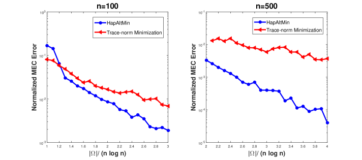
Figure 2: A comparison of the normalized minimum error correction score of Algorithm 3 and the trace-norm minimization (SVT) method for matrices of dimensions $n=100$ and $n=500$, plotted as a function of sample size. $\alpha$ is $2$ and error probability $p_{e}$ is set to $5\%$. The values shown are averaged over $100$ simulation runs.

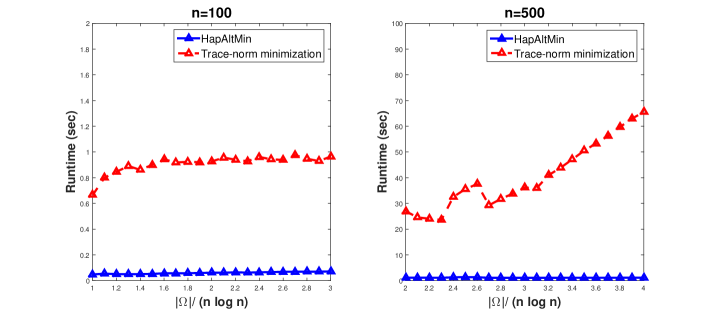
Figure 3: A comparison of the runtime of Algorithm 3 and the trace-norm minimization (SVT) method for matrices of dimensions $n=100$ and $n=500$, plotted as a function of sample size. $\alpha$ is $2$ and error probability $p_{e}$ is set to $5\%$. The values shown are averaged over $100$ simulation runs.

In Figure 2 we compare the MEC error rate performance of Algorithm 3 (denoted as HapAltMin in the figure) with another matrix completion approach, namely singular value thresholding (SVT) [40]; SVT is a widely used trace-norm minimization based method. We compare their performance on randomly generated binary rank-one matrices of size $50\times 100$ and $250\times 500$, and flip the entries in a uniformly randomly chosen sample set $\Omega$ with probability $0.05$. Both methods are run $100$ times for each chosen sample size and error rates are averaged over those runs. Results of the trace-norm minimization method are rounded off in the final iterations. Figure 2 suggests that alternating minimization based matrix completion approach performs better than the trace-norm minimization based method for both problem dimensions, and the performance gap is wider for $n=500$ compared to $n=100$. Figure 3 plots the runtime of the two methods for the same problem instances. Trace-norm minimization based method, that was reported in literature as the most accurate version of SVT, is much slower of the two, primarily due to the computationally expensive SVD operation at each iteration step.

Next, we present the analysis frameworks for the initial and subsequent iterative steps of Algorithm 3.

IV-A Initialization Analysis

In order for Algorithm 3 to converge, a suitable initial starting point close to the ground truth is necessary. In addition to the power iteration step, which gives a singular vector that is close to the true vector ${\bf u}^{\star}$, the subsequent clipping step helps retain the incoherence of the same, without sacrificing the closeness property. The following lemma uses Theorem 3 to establish the incoherence of $\hat{{\bf u}}^{(0)}$, and that $\hat{{\bf u}}^{(0)}$ remains close to the true left singular vector ${\bf u}^{\star}$.

Lemma 3.

Let ${\bf u}^{(0)}$ be obtained after normalizing the output of the power iteration step in Algorithm 3. Let ${\bf u}^{C}$ be the vector obtained after setting entries of ${\bf u}^{(0)}$ greater than $2\frac{\mu}{\sqrt{m}}$ to zero. If $\tilde{{\bf u}}$ is the normalized ${\bf u}^{C}$, then, with high probability, we have $\text{dist}(\tilde{{\bf u}},{\bf u}^{\star})\leq 1/2$, and $\tilde{{\bf u}}$ is incoherent with parameter $4\mu$, where $\mu$ is the incoherence parameter of ${\bf u}^{\star}$.

Proof.

The proof follows directly from Lemma C.2 from [24] and Lemma 2 from [27] after suitably using conditions from Lemma 1 and Theorem 3. ∎

IV-B Convergence Analysis

Let us denote $\lambda_{j}=\frac{1}{m}\sum\limits_{i|(i,j)\in\Omega}R_{ij}u_{i}^{(t)}$. The Taylor series expansion of $\hat{v}_{j}^{(t+1)}$ from (17) is given by

$${\hat{v}}_{j}^{(t+1)} =\frac{\lambda_{j}}{2}-\frac{{\lambda_{j}}^{3}}{24}+\frac{{\lambda_{j}}^{5}}{240}-\ldots,~{}~{}~{}\forall~{}j=1,\ldots,n.$$ (22)

Now, we have

$$|\lambda_{j}|=\left|\frac{1}{m}\sum\limits_{i|(i,j)\in\Omega}R_{ij}u_{i}^{(t)}\right|\leq\frac{1}{m}\sum\limits_{i|(i,j)\in\Omega}|R_{ij}||u_{i}^{(t)}|\leq\frac{1}{m}\sum\limits_{i|(i,j)\in\Omega}|R_{ij}|.$$

Clearly, $\sum\limits_{i|(i,j)\in\Omega}|R_{ij}|\sim\text{Bin}(m,p)$ for a given $j$, implying that the absolute value of $\lambda_{j}$ is close to the entry-wise observation probability $p<1$. This, in turn, implies that in (22) all terms with higher powers of $\lambda_{j}$ are much smaller than the dominant linear term, and the Taylor’s series expansion can be written as ${\hat{v}}_{j}^{(t+1)}\approx\frac{\lambda_{j}}{2}+\epsilon(\lambda_{j})$, where the error term $\epsilon(\lambda_{j})$ can be bounded as $|\epsilon(\lambda_{j})|\leq|\lambda_{j}|^{3}/3!\ll 1$ using the Lagrange error bound. Therefore, we approximate the update in (17) as

$$\begin{split}{\hat{v}}_{j}^{(t+1)}&=\frac{1}{2m}\sum\limits_{i|(i,j)\in\Omega}R_{ij}u_{i}^{(t)}\\ &=\frac{1}{2m}\sum\limits_{i|(i,j)\in\Omega}(M_{ij}+N_{ij})u_{i}^{(t)}\\ &=\frac{1}{2m}\sum\limits_{i|(i,j)\in\Omega}\left(\sigma^{\star}u_{i}^{\star}v_{j}^{\star}+[{\bf U}_{N}^{(i)}]^{T}\Sigma_{N}{\bf V}_{N}^{(j)}\right)u_{i}^{(t)}\\ &=\frac{1}{2m}\left(\sigma^{\star}\langle{\bf u}^{(t)},{\bf u}^{\star}\rangle v_{j}^{\star}-\left[\sigma^{\star}\langle{\bf u}^{(t)},{\bf u}^{\star}\rangle v_{j}^{\star}\right.\right.\\ &\quad\left.\left.-\sigma^{\star}v_{j}^{\star}\sum\limits_{i|(i,j)\in\Omega}u_{i}^{(t)}u_{i}^{\star}\right]+\sum\limits_{i|(i,j)\in\Omega}u_{i}^{(t)}[{\bf U}_{N}^{(i)}]^{T}\Sigma_{N}{\bf V}_{N}^{(j)}\right)\end{split}$$ (23)

for $j=1,\ldots,n$.

Let us introduce an error vector ${\bf F}\in\mathbb{R}^{n}$ as ${\bf F}=\sigma^{\star}{\bf B}^{-1}\left(\langle{\bf u}^{(t)},{\bf u}^{\star}\rangle{\bf B}-{\bf C}\right){\bf v}^{\star}$, where ${\bf B}=\frac{1}{p}\mathbb{I}_{n}$ and ${\bf C}\in\mathbb{R}^{n\times n}$ is diagonal with $C_{jj}=\frac{1}{p}\sum\limits_{i|(i,j)\in\Omega}u_{i}^{(t)}u_{i}^{\star},~{}\forall j=1,\ldots,n$. Furthermore, let us define a noise vector $N_{\text{res}}\in\mathbb{R}^{n\times 1}$ as $N_{\text{res}}={\bf B}^{-1}{\bf C}^{N}{\bf S}^{N}{\bf v}^{N}$, where the quantities are as follows:

• ${\bf C}^{N}=[{\bf C}_{1}^{N}~{}{\bf C}_{2}^{N}\cdots{\bf C}_{m}^{N}]\in\mathbb{R}^{n\times nm}$ where $({\bf C}_{q}^{N})_{jj}=\frac{1}{p}\sum\limits_{i|(i,j)\in\Omega}u_{i}^{(t)}{\bf U}_{iq}^{N},~{}~{}\forall q\in[m],\forall j\in[n]$;

• ${\bf S}^{N}\in\mathbb{R}^{nm\times nm}$ is a diagonal matrix given by ${\bf S}^{N}=\text{diag}\left(\sigma_{1}^{N}\mathbb{I}_{n},\ldots,\sigma_{m}^{N}\mathbb{I}_{n}\right)$;

• ${\bf v}^{N}=\left[({\bf v}_{1}^{N})^{T}~{}({\bf v}_{2}^{N})^{T}~{}\ldots~{}({\bf v}_{m}^{N})^{T}\right]^{T}\in\mathbb{R}^{nm\times 1}$ where ${\bf v}_{j}^{N}\in\mathbb{R}^{n}$ is the $j^{th}$ column of ${\bf V}_{N}$.

We also define $C_{jj}^{N}=\left[({\bf C}_{1}^{N})_{jj}~{}({\bf C}_{2}^{N})_{jj}~{}\ldots~{}({\bf C}_{m}^{N})_{jj}\right]$ for any given $j\in[n]$. Using the above definitions, (23) can be written as

$$\hat{v}_{j}^{(t+1)}=\frac{1}{2m}\left[\sigma^{\star}\langle{\bf u}^{(t)},{\bf u}^{\star}\rangle v_{j}^{\star}-F_{j}+\frac{1}{B_{jj}}C_{jj}^{N}\Sigma_{N}{\bf V}_{N}^{(j)}\right].$$ (24)

Therefore, using vector-matrix notation, the update of $\hat{{\bf v}}$ can be written as

$${\hat{{\bf v}}}^{(t+1)} =\frac{1}{2m}\left[\sigma^{\star}\langle{\bf u}^{(t)},{\bf u}^{\star}\rangle{\bf v}^{\star}-{\bf F}+N_{\text{res}}\right]$$ (25)

$$=\frac{1}{2m}\left[{\bf M}^{T}{\bf u}^{(t)}-{\bf F}+N_{\text{res}}\right].$$

Recalling (11), one can identify that ${\bf M}^{T}{\bf u}^{(t)}$ in the above expression is the update term in the power iteration applied to the true matrix ${\bf M}$. Therefore, the update described in (25) is essentially power iteration of ${\bf M}$ that would have led to the true singular vector ${\bf u}^{\star}$ except that it is perturbed by error terms due to incomplete observations and sequencing noise (${\bf F}$ and $N_{\text{res}}$ in the above expression, respectively). This observation leads to the analysis approach where appropriate upper bounds to the aforementioned errors terms are derived. The proof of convergence presented in this work follows the framework adopted in [24, 27], and consists of an inductive analysis based on establishing the guarantee that, given ${\bf u}^{(t)}$ is incoherent and has a small distance in terms of principal angle with respect to ${\bf u}^{\star}$, the subsequent iterate ${\bf v}^{(t+1)}$ is also incoherent with identical parameter, and is closer to ${\bf v}^{\star}$ by at least a constant factor. This statement is formally expressed using Theorem 2 and Lemma 4 for the distance and incoherence conditions, respectively.

Theorem 2.

Under the assumptions of Theorem 1, the $(t+1)^{th}$ iterates $\hat{{\bf u}}^{(t+1)}$ and $\hat{{\bf v}}^{(t+1)}$ of Algorithm 3 satisfy with high probability

$$\text{dist}(\hat{{\bf v}}^{(t+1)},{\bf v}^{\star}) \leq\frac{1}{4}\text{dist}(\hat{{\bf u}}^{(t)},{\bf u}^{\star})+\frac{\mu_{1}p_{e}}{\delta_{2}},~{}~{}\text{and}$$

$$\text{dist}(\hat{{\bf u}}^{(t+1)},{\bf u}^{\star}) \leq\frac{1}{4}\text{dist}(\hat{{\bf v}}^{(t+1)},{\bf v}^{\star})+\frac{\mu_{1}p_{e}}{\delta_{2}},~{}0\leq t\leq T-1,$$

where $\mu_{1}$ is the incoherence parameter of the intermediate iterates $\hat{{\bf u}}^{(t)}$ and $\hat{{\bf v}}^{(t)}$.

We defer the proofs of both Theorem 1 and Theorem 2 to Appendix A. Theorem 2 is a starting point for proving Theorem 1, and establishes a geometric decay of the distance between the subspaces spanned by $(\hat{{\bf u}}^{(t)}$, $\hat{{\bf v}}^{(t)})$ and $({\bf u}^{\star}$, ${\bf v}^{\star})$ respectively. Next, we present a corollary based on the findings of Theorem 2.

Corollary 2.

Under the assumptions of Theorem 2, at the end of $T=\mathcal{O}(\log\frac{\|{\bf M}\|_{F}}{\epsilon})$ iterations, it holds that

$$\text{dist}(\hat{{\bf v}}^{(T+1)},{\bf v}^{\star}) \leq\frac{1}{2}\frac{\epsilon}{\|{\bf M}\|_{F}}+\frac{4\mu_{1}p_{e}}{3\delta_{2}},~{}~{}\text{and}$$

$$\text{dist}(\hat{{\bf u}}^{(T+1)},{\bf u}^{\star}) \leq\frac{1}{2}\frac{\epsilon}{\|{\bf M}\|_{F}}+\frac{4\mu_{1}p_{e}}{3\delta_{2}}.$$

Proof.

It follows from Theorem 2 that, after $T$ iterations,

$$\begin{split}\text{dist}(\hat{{\bf u}}^{(T)},{\bf u}^{\star})&\leq\frac{1}{4}\left(\frac{1}{4}\text{dist}(\hat{{\bf u}}^{(T-1)},{\bf u}^{\star})+\frac{\mu_{1}p_{e}}{\delta_{2}}\right)+\frac{\mu_{1}p_{e}}{\delta_{2}}\\ &=\frac{1}{16}\text{dist}(\hat{{\bf u}}^{(T-1)},{\bf u}^{\star})+\frac{5\mu_{1}p_{e}}{4\delta_{2}}\\ &\vdots\\ &\leq\frac{1}{16^{T}}\text{dist}(\hat{{\bf u}}^{(0)},{\bf u}^{\star})+\frac{5\mu_{1}p_{e}}{4\delta_{2}}\left(1+\frac{1}{16}\frac{1}{16^{2}}++\cdots\text{(T terms)}\right)\\ &\overset{\zeta_{1}}{\leq}\frac{1}{2}\frac{1}{16^{T}}+\frac{4\mu_{1}p_{e}}{3\delta_{2}}\\ &\leq\frac{1}{2}\frac{\epsilon}{\|{\bf M}\|_{F}}+\frac{4\mu_{1}p_{e}}{3\delta_{2}},~{}\text{as}~{}T=\mathcal{O}\left(\log\frac{\|{\bf M}\|_{F}}{\epsilon}\right)\end{split}$$

where $\zeta_{1}$ follows from the fact that $\text{dist}(\hat{{\bf u}}^{(0)},{\bf u}^{\star})\leq 1/2$ (see Lemma 3). ∎

Corollary 2 is used to complete the proof of Theorem 1 in Appendix A. The following lemma states the incoherence condition; we defer its proof to Appendix A.

Lemma 4.

Let ${\bf M},{\bf N}$, $p$, $\Omega$ be defined as in Theorem 1. Let ${\bf u}^{(t)}$ be the unit vector obtained at the $t^{th}$ iteration of Algorithm 3 with incoherence parameter $\mu_{1}=8\mu$. Then, with probability greater than $1-1/n^{3}$, the next iterate ${\bf v}^{(t+1)}$ is also $\mu_{1}$ incoherent.

Remark 5: In our analysis of the matrix factorization approach to single individual haplotyping, we adopted techniques proposed by [24, 27]; note, however, that the scope of analysis in the current paper goes beyond the prior works. In particular, the authors of [24] considered a noiseless case of matrix factorization and did not impose structural constraints on the iterates. Their work was extended to a noisy case in [27] for a similar unconstrained setting. Additionally, [27] did not exploit statistical properties of the noise, except the entry-wise upper bound, whereas the present work uses the bit-flipping model as discussed in Section II-C, which allows us to characterize the dependence of the performance on the sequencing error probability $p_{e}$.

V Results and Discussions

We begin this section by stating the metrics for evaluating performance of our single individual hapolotyping algorithm.

V-A Performance Metrics

A widely used metric for characterizing the quality of single individual haplotyping is the minimum error correction (MEC) score. This metric captures the smallest number of entries of $P_{\Omega}({\bf R})$ which need to be changed from $1$ to $-1$ and vice versa so that $P_{\Omega}({\bf R})$ can be interpreted as a noiseless version of $P_{\Omega}({\bf M})$. Essentially, it is the most likely number of sequencing errors, defined for diploids as

MEC $$=\sum\limits_{i=1}^{n}~{}\min\left(D(r_{i},\hat{h}_{1}),D(r_{i},\hat{h}_{-1})\right),$$ (26)

where $D(r_{i},\hat{h}_{j})$ denotes the generalized Hamming distance between read $r_{i}$ (regarded as $m$ length vector in $\{1,-1,\text{`-'}\}$) and the estimated parent haplotypes $\hat{h}_{k},~{}k=1,-1$. This, in turn, is defined as $D(r_{i},\hat{h}_{j})=\sum_{j=1}^{m}~{}d(r_{i,j},\hat{h}_{k,j})$, where

$$d(x,y)=\begin{cases}1,&~{}\text{if}~{}x\neq\text{`-' ~{}and ~{}}y\neq\text{`-' ~{}and ~{}}x\neq y\\ 0,&~{}\text{otherwise},\end{cases}$$ (27)

and $r_{i,j}$ and $\hat{h}_{k,j}$ denote the $j^{th}$ entries of $r_{i}$ and $\hat{h}_{k}$, respectively.

The MEC score is a relevant and most commonly studied performance metric for single individual haplotyping [41], and critically important for experimental data where the ground truth is not known in advance. It is also a proxy for the most meaningful haplotype assembly metric referred to as reconstruction rate. Recall that $\mathcal{H}=\{h_{1},h_{-1}\}$ denotes the set of true haplotypes. Then the reconstruction rate of $\hat{\mathcal{H}}=\{\hat{h}_{1},\hat{h}_{-1}\}$ with respect to $\mathcal{H}$ is defined as [42]

$$\mathcal{R}_{\mathcal{H},\hat{\mathcal{H}}}=1-\frac{\min\{D(h_{1},\hat{h}_{1}+D(h_{-1},\hat{h}_{-1}),D(h_{1},\hat{h}_{-1})+D(h_{-1},\hat{h}_{1})\}}{2m},$$ (28)

where $D(h_{i},h_{j})$ denotes the generalized Hamming distance between the haplotype pair $h_{i}$ and $h_{j}$.

V-B Experiments

In this section, for convenience we refer to our algorithm for single individual haplotyping as HapAltMin . All of the methods described here were run on a Linux OS desktop with 3.07 GHz CPU and 8 GB RAM on an Intel Core i7 880 Processor.

We first tested our algorithm on the experimental dataset containing Fosmid pool-based NGS data for HapMap trio child $NA12878$ [12]. The Fosmid dataset is characterized by very long fragments, high SNP to read ratio, and low sequencing coverage of about 3X, consisting of around $1,342,091$ SNPs spread across $22$ chromosomes. We compare the performance of HapAltMin with the structurally-constrained gradient descent (SCGD) algorithm of [18] and one more recent SIH software ProbHap [16], which was shown to be superior to several prior methods on this dataset [10, 12, 17]. Table I shows the MEC rate (average number of mismatches per SNP position across the reads) and runtimes for all $22$ chromosomes. As seen there, our HapAltMin outperforms other methods for majority of the chromosomes shown; it is second best in terms of runtime (behind SCGD).

TABLE I: MEC rates and runtimes on HapMap sample NA12878 dataset.

Chr	HapAltMin		SCGD		ProbHap
	MEC	time(s)	MEC	time(s)	MEC	time(s)
1	0.034	65.0	0.04	44.2	0.058	87.7
2	0.035	71.6	0.035	49.5	0.055	88.9
3	0.034	61.1	0.036	41.5	0.057	84.3
4	0.029	60.7	0.034	41.8	0.053	67.1
5	0.032	52.9	0.036	39.9	0.054	64.6
6	0.038	34.7	0.037	27.9	0.050	53.4
7	0.038	26.4	0.035	25.05	0.055	40.8
8	0.033	24.3	0.034	23.9	0.05	42.8
9	0.036	21.9	0.037	17.6	0.052	45.2
10	0.036	24.7	0.037	21.0	0.053	44.4
11	0.034	24.7	0.038	20.8	0.055	39.5
12	0.037	23.5	0.037	20.2	0.057	38.9
13	0.039	14.6	0.035	15.6	0.053	26.4
14	0.035	16.6	0.039	13.7	0.055	27.4
15	0.038	14.1	0.041	11.9	0.056	26.5
16	0.046	20.3	0.0405	12.2	0.051	36.5
17	0.048	15.3	0.046	11.1	0.061	27.4
18	0.033	12.2	0.037	11.8	0.053	24.4
19	0.052	12.8	0.046	9.0	0.063	19.8
20	0.044	18.1	0.044	13.0	0.055	30.9
21	0.035	11.5	0.041	8.5	0.051	15.6
22	0.054	11.7	0.055	8.6	0.061	31.4

TABLE II: MEC rate comparison of Algorithm 2 and Algorithm 3.

Chr	Algorithm 2 (“Hard” updates)	Algorithm 3 (“Soft” updates)
1	0.0369	0.0339
2	0.0357	0.035
3	0.0345	0.0335
20	0.0447	0.0446
21	0.0367	0.035
22	0.0568	0.0535

We further compare the MEC performance of Algorithm 3 with that of the discrete version (Algorithm 2) in Table II for first $3$ and last $3$ of the $22$ chromosomes from the Fosmid dataset. As can be seen from Table II, the modified algorithm performs better than the discrete alternating minimization algorithm, as indicated in the discussion in Section III.

Next, we focus on the evaluation of performance on simulated dataset using reconstruction rate metric. For this purpose, we use a widely popular standard benchmarking dataset from [42] which also provides the true haplotypes used to generate the read data. The dataset contains reads at a sequencing error rate with values in the set $\{0.0,0.1,0.2,0.3\}$, and a depth of coverage in the set $\{3X,5X,8X,10X\}$. Reconstruction rate of our algorithm is compared with that of SCGD [18] and two more recent SIH methods known as HGHap [43] and MixSIH [17]. In particular, [43] is chosen for performance comparison since it has been shown to outperform a number of existing SIH methods such as [9, 44, 10, 45, 46]. A comparison with ProbHap is not shown for this data since it reconstructed haplotypes with a large fraction of SNPs missing (and therefore has inferior performance compared to the methods used in the comparisons). The results, shown in Table III, are obtained by averaging over $100$ simulation runs for each combination of sequencing error rate and sequencing coverage, for a haplotype length of $700$ base pairs and pairwise hamming distance $0.7$. As evident from the results, our method is either the best or the second best in all of the scenarios. HapAltMin performs particularly well in the more realistic error range of $0.0-0.2$ and is marginally inferior to MixSIH only for higher sequencing error values.

TABLE III: Reconstruction rate comparison on simulated data. Boldface values indicate best performance.

Error Rate	Cov.	HapAltMin	SCGD	HGHap	MixSIH
0.0	3X	1	0.983	0.934	0.776
0.0	5X	1	0.976	0.989	0.923
0.0	8X	1	0.999	0.994	0.995
0.0	10X	1	0.999	0.999	1
0.1	3X	0.935	0.869	0.934	0.775
0.1	5X	0.979	0.951	0.990	0.942
0.1	8X	0.996	0.996	0.987	0.972
0.1	10X	0.999	0.999	0.997	0.993
0.2	3X	0.735	0.677	0.677	0.68
0.2	5X	0.864	0.785	0.91	0.774
0.2	8X	0.943	0.899	0.884	0.932
0.2	10X	0.966	0.934	0.894	0.969
0.3	3X	0.555	0.527	0.592	0.65
0.3	5X	0.595	0.524	0.621	0.667
0.3	8X	0.68	0.518	0.646	0.714
0.3	10X	0.723	0.58	0.696	0.751

VI Conclusion

Motivated by the single individual haplotyping problem from computational biology, we proposed and analyzed a binary-constrained variant of the alternating minimization algorithm for solving the rank-one matrix factorization problem. We provided theoretical guarantees on the performance of the algorithm and analyzed its required sample probability; the latter has important implications on experimental specifications, namely, sequencing coverage. Performance of haplotype reconstruction is often expressed in terms of the minimum error correction score; we establish theoretical guarantees on the achievable MEC score for the proposed binary-constrained alternating minimization. Experiments with a HapMap sample NA12878 dataset as well as those with a widely used benchmarking simulated dataset demonstrated efficacy of our algorithm.

Appendix A Proofs of Lemmas and Theorems

A-A Preliminaries

The following property and lemma are well-known classical results that will be useful in the forthcoming proofs.

Property 1.

For a given matrix ${\bf M}\in\mathbb{R}^{m\times n}$ of rank $k$, the following relations hold between the 2-norm, the Frobenius norm and the entry-wise $\ell_{1}$ norm of ${\bf M}$:

• $\|{\bf M}\|_{2}\leq\|{\bf M}\|_{F}\leq\sqrt{k}\|{\bf M}\|_{2}$

• $\|{\bf M}\|_{F}\leq\|{\bf M}\|_{1}\leq\sqrt{mn}\|{\bf M}\|_{F}$

Lemma 5 (Bernstein’s inequality).

Let $X_{1},X_{2},\ldots,X_{n}$ be independent random variables. Also, let $|X_{i}|\leq L\in\mathbb{R}~{}\forall i$ w.p. 1. Then it holds that

$$Pr\left(\left|\sum\limits_{i=1}^{n}X_{i}-\sum\limits_{i=1}^{n}\mathbb{E}[X_{i}]\right|>t\right)\leq 2\exp\left(-\frac{t^{2}/2}{Lt/3+\sum\limits_{i=1}^{n}\text{Var}(X_{i})}\right).$$

The following theorem from [25] provides an upper bound on the error between the true matrix ${\bf M}$ and the best rank-$k$ approximation of the noisy and partially observed version of ${\bf M}$, and is used in the proof of Lemma 3.

Theorem 3.

[25] Let ${\bf R}={\bf M}+{\bf N}$, where ${\bf M}$ is an $m\times n$ $\mu$-incoherent matrix with rank $k$ ($m\leq n$) and the indices in the sampling set $\Omega\in[m]\times[n]$ are chosen uniformly at random. Let $\alpha=n/m$, $|M_{ij}|\leq M_{\max}$ and $p$ be the sampling probability. Furthermore, from the SVD of  $\frac{1}{p}P_{\Omega}({\bf R})$, we get a rank-$k$ approximation given by $[P_{\Omega}({\bf R})]_{k}={{\bf U}}^{0}{\Sigma}^{0}({{\bf V}}^{0})^{T}$. Then there exists numerical constants $C$ and $C^{\prime}$ such that, with probability greater than $1-\frac{1}{n^{3}}$, we have

$$\frac{1}{\sqrt{mn}}\|{\bf M}-[{P}_{\Omega}({\bf R})]_{k}\|_{2}\leq CM_{\max}\left(\frac{m\alpha^{3/2}}{|\Omega|}\right)^{1/2}+\frac{C^{\prime}m\sqrt{\alpha}}{|\Omega|}\|{P}_{\Omega}({\bf N})\|_{2}.$$

A-B Induction Proofs

Lemma 6.

Let ${\bf M},{\bf N},\Omega$ and ${\bf u}^{(t)}$ be defined as in Algorithm 3. Then, with high probability we have

$$\|{\bf F}\|_{2}\leq\sigma^{\star}\delta_{2}\sqrt{1-{\langle{\bf u}^{(t)},{\bf u}^{\star}\rangle}^{2}}.$$

Proof.

From the definition of ${\bf F}$ stated in Section IV-B, we have

$$\|{\bf F}\|_{2} \leq\sigma^{\star}\|{\bf B}^{-1}\|_{2}\|\left({\bf C}-{\langle{\bf u}^{(t)},{\bf u}^{\star}\rangle}{\bf B}\right){\bf v}^{\star}\|_{2}.$$ (29)

Since ${\bf B}$ is a diagonal matrix, $\|{\bf B}^{-1}\|_{2}=\frac{1}{\min_{i}B_{ii}}=p\leq 1$. Let ${\bf x}\in\mathbb{R}^{n}$ be such that $\|{\bf x}\|_{2}=1$. Then, for all such ${\bf x}$,

$$\begin{split}&{\bf x}^{T}\left({{\bf C}-\langle{\bf u}^{(t)},{\bf u}^{\star}\rangle}\mathbb{I}\right){\bf v}^{\star}\\ &\quad=\frac{1}{p}\sum\limits_{j}x_{j}v_{j}^{\star}\left(\sum\limits_{i|ij\in\Omega}u_{i}^{(t)}u_{i}^{\star}-\langle{\bf u}^{(t)},{\bf u}^{\star}\rangle\right)\\ &\quad\leq\frac{1}{p}\sum\limits_{ij\in\Omega}x_{j}v_{j}^{\star}\left(u_{i}^{(t)}u_{i}^{\star}-{\langle{\bf u}^{(t)},{\bf u}^{\star}\rangle(u_{i}^{(t)})^{2}}\right)\\ &\quad\overset{\zeta_{1}}{\leq}\frac{C}{p}\sqrt{np}\sqrt{\sum\limits_{j}x_{j}^{2}(v_{j}^{\star})^{2}}\sqrt{\sum\limits_{i}\left(u_{i}^{(t)}u_{i}^{\star}-{\langle{\bf u}^{(t)},{\bf u}^{\star}\rangle(u_{i}^{(t)})^{2}}\right)^{2}}\\ &\quad\overset{\zeta_{2}}{\leq}\frac{C}{p}\sqrt{np}\sqrt{\frac{\mu_{1}^{2}}{n}\sum\limits_{j}x_{j}^{2}}~{}\sqrt{\sum\limits_{i}(u_{i}^{(t)})^{2}\left(u_{i}^{\star}-{\langle{\bf u}^{(t)},{\bf u}^{\star}\rangle u_{i}^{(t)}}\right)^{2}}\\ &\quad\overset{\zeta_{3}}{\leq}\frac{C}{p}\frac{\sqrt{np}\mu_{1}^{2}}{\sqrt{mn}}\sqrt{1-{\langle{\bf u}^{(t)},{\bf u}^{\star}\rangle}^{2}}\\ &\quad\leq\delta_{2}\sqrt{1-{\langle{\bf u}^{(t)},{\bf u}^{\star}\rangle}^{2}},\qquad\text{if}~{}~{}p\geq C^{\prime}\frac{\mu_{1}^{4}}{m\delta_{2}^{2}},\end{split}$$

where $C^{\prime}=C^{2}>0$ is a global constant and $\zeta_{1}$ follows from Lemma 7 (which imposes the condition $p\geq C\frac{\log n}{m}$) and $\zeta_{2}$ follows from the incoherence of ${\bf v}^{\star}$, and $\zeta_{3}$ from that of ${\bf u}^{(t)}$. Then,

$$\|\left({{\bf C}-\langle{\bf u}^{(t)},{\bf u}^{\star}\rangle}{\bf B}\right){\bf v}^{\star}\|_{2} =\underset{\|{\bf x}\|_{2}=1}{\max}~{}{\bf x}^{T}\left({{\bf C}-\langle{\bf u}^{(t)},{\bf u}^{\star}\rangle}{\bf B}\right){\bf v}^{\star}$$

$$\leq\delta_{2}\sqrt{1-{\langle{\bf u}^{(t)},{\bf u}^{\star}\rangle}^{2}}.$$

Hence, the lemma follows from (29) if $p\geq C^{\prime}\frac{\mu_{1}^{4}\log n}{m\delta_{2}^{2}}$. ∎

Lemma 7.

([24]) Let $\Omega\in[m]\times[n]$ be a set of indices sampled uniformly at random with sampling probability $p$ that satisfies $p\geq C\frac{\log n}{m}$. Then with probability $\geq 1-\frac{1}{n^{3}}$ $\forall{\bf x}\in\mathbb{R}^{m},\forall{\bf y}\in\mathbb{R}^{n}$ such that ${\bf x}$ satisfies $\sum_{i}x_{i}=0$, it holds that $\sum\limits_{ij\in\Omega}x_{i}y_{j}\leq C\sqrt{\sqrt{mn}p}\|{\bf x}\|_{2}\|{\bf y}\|_{2}$, where $C>0$ is a global constant.

Lemma 8.

Let ${\bf M},{\bf N},\Omega$ and $p_{e}$ be defined as before. Then with high probability it holds that

$$\|N_{\text{res}}\|_{2}\leq 2N_{\max}\mu_{1}p_{e}\sqrt{mn}.$$

Proof.

The proof follows from Lemma B.3, [27] for the case $k=1$, and by noting the fact that $\|{\bf B}^{-1}\|_{2}\leq 1$, and from the observation that $\frac{\|\mathcal{P}_{\Omega}({\bf N})\|_{2}}{p}\leq 2N_{\max}p_{e}\sqrt{mn},~{}\text{with high probability}$ (see Lemma 1). ∎

Lemma 9.

Let ${\bf F}$, $N_{\text{res}}$ and ${\bf u}^{(t)}$ be defined as in (25). Then we have

$$\|{\hat{{\bf v}}}^{(t+1)}\|_{2}\geq\frac{1}{2m}\left(\sigma^{\star}\sqrt{1-\text{dist}^{2}({\bf u}^{\star},{\bf u}^{(t)})}-\|{\bf F}\|_{2}-\|N_{\text{res}}\|_{2}\right).$$

Proof.

$$2m\|{\hat{{\bf v}}}^{(t+1)}\|_{2} =\|\sigma^{\star}\langle{\bf u}^{(t)},{\bf u}^{\star}\rangle{\bf v}^{\star}-{\bf F}+N_{\text{res}}\|_{2}$$

$$\overset{\zeta_{1}}{\geq}\|\sigma^{\star}\langle{\bf u}^{(t)},{\bf u}^{\star}\rangle{\bf v}^{\star}\|_{2}-\|{\bf F}-N_{\text{res}}\|_{2}$$

$$\overset{\zeta_{2}}{\geq}\|\sigma^{\star}\langle{\bf u}^{(t)},{\bf u}^{\star}\rangle{\bf v}^{\star}\|_{2}-\|{\bf F}\|_{2}-\|N_{\text{res}}\|_{2}$$

$$=\sigma^{\star}\sqrt{1-\text{dist}^{2}({\bf u}^{\star},{\bf u}^{(t)})^{2}}-\|{\bf F}\|_{2}-\|N_{\text{res}}\|_{2},$$

where both $\zeta_{1}$ and $\zeta_{2}$ follow from the reverse triangle inequality for vectors. ∎

Lemma 10.

Under the conditions of Theorem 1, with probability greater than $1-1/n^{3}$ it holds that for a given $j\in[n]$,

$$\left|\frac{1}{B_{jj}}C_{jj}^{N}\Sigma_{N}{\bf V}_{N}^{(j)}\right| \leq N_{\max}\mu_{1}\sqrt{m}(p_{e}+\delta_{2}).$$

Proof.

Let a Bernoulli random variable $\delta_{ij}$ characterize the event that the $(i,j)$ entry in ${\bf R}$ is observed and is in error. Therefore, $\delta_{ij}=1$ w.p. $pp_{e}$ and $0$ otherwise. Also, let us define $Z_{i}=\frac{1}{p}\delta_{ij}u_{i}^{(t)}N_{\max}$ and $Z=\sum_{i=1}^{m}~{}Z_{i}$. Then,

$$\mathbb{E}[Z]=\mathbb{E}\left[\sum_{i=1}^{m}~{}Z_{i}\right] =p_{e}\sum_{i=1}^{m}~{}u_{i}^{(t)}N_{\max}\overset{\zeta_{1}}{\leq}N_{\max}p_{e}\mu_{1}\sqrt{m},$$

where $\zeta_{1}$ follows from the incoherence of $u_{i}^{(t)}$. Moreover,

$$\text{Var}(Z)=\frac{p_{e}}{p}(1-pp_{e})N_{\max}^{2}\sum_{i=1}^{m}|u_{i}^{(t)}|^{2}\leq N_{\max}^{2}\frac{p_{e}}{p}(1-pp_{e})\leq N_{\max}^{2}\frac{p_{e}}{p},$$

and $\max_{i}~{}|Z_{i}|=\frac{1}{p}\max_{i}~{}|u_{i}^{(t)}N_{ij}|\leq\frac{\mu_{1}N_{\max}}{p\sqrt{m}}$. Using Bernstein’s inequality, we have

$$\begin{split}&Pr\left(Z-\mathbb{E}[Z]>N_{\max}\mu_{1}\sqrt{m}\delta_{2}\right)\\ &\qquad\leq\exp\left(-\frac{N_{\max}^{2}\mu_{1}^{2}m\delta_{2}^{2}/2}{N_{\max}^{2}\frac{p_{e}}{p}+\frac{N_{\max}\mu_{1}}{3p\sqrt{m}}N_{\max}\mu_{1}\sqrt{m}\delta_{2}}\right)\\ &\qquad=\exp\left(-\frac{p\mu_{1}^{2}m\delta_{2}^{2}/2}{p_{e}+\frac{\mu_{1}^{2}\delta_{2}}{3}}\right)\overset{\zeta_{2}}{\leq}\exp\left(-3\log n\right)=\frac{1}{n^{3}},\end{split}$$

where $\zeta_{2}$ follows by using the condition from Theorem  1 that $p>\frac{6\log n}{\mu_{1}^{2}m\delta_{2}^{2}}(p_{e}+\frac{\mu_{1}^{2}\delta_{2}}{3})$.

Therefore, using the definition from (24), with probability greater than $1-1/n^{3}$ it holds that

$$\left|\frac{1}{B_{jj}}C_{jj}^{N}\Sigma_{N}{\bf V}_{N}^{(j)}\right|=\left|\frac{1}{p}\sum\limits_{i|ij\in\Omega}u_{i}^{(t)}[{\bf U}_{N}^{(i)}]^{T}\Sigma_{N}{\bf V}_{N}^{(j)}\right|=\left|\frac{1}{p}\sum\limits_{i|ij\in\Omega}u_{i}^{(t)}N_{ij}\right|\leq N_{\max}\mu_{1}\sqrt{m}(p_{e}+\delta_{2}).$$

∎

Proof of Lemma 4.

We bound the largest magnitude of the entries of $\hat{{\bf v}}^{(t+1)}$ as follows. For every $j\in[n]$, using (24) we have

$$\begin{split}&2m\left|\hat{v}_{j}^{(t+1)}\right|\leq|\sigma^{\star}\langle{\bf u}^{(t)},{\bf u}^{\star}\rangle v_{j}^{\star}|\\ &\quad+\left|\frac{\sigma^{\star}}{B_{jj}}(\langle{\bf u}^{(t)},{\bf u}^{\star}\rangle B_{jj}-C_{jj})v_{j}^{\star}\right|+\left|\frac{1}{B_{jj}}C_{jj}^{N}\Sigma_{N}{\bf V}_{N}^{(j)}\right|\\ &\quad\overset{\zeta_{1}}{\leq}\sigma^{\star}\langle{\bf u}^{(t)},{\bf u}^{\star}\rangle\frac{\mu}{\sqrt{n}}+\sigma^{\star}\langle{\bf u}^{(t)},{\bf u}^{\star}\rangle\frac{\mu}{\sqrt{n}}\\ &\quad+\sigma^{\star}(\langle{\bf u}^{(t)},{\bf u}^{\star}\rangle+\delta_{2})\frac{\mu}{\sqrt{n}}+N_{\max}\mu_{1}\sqrt{m}(p_{e}+\delta_{2})\\ &\quad\overset{\zeta_{2}}{\leq}\sigma^{\star}(3+\delta_{2})\frac{\mu}{\sqrt{n}}+N_{\max}\sigma^{\star}\frac{\mu_{1}}{\sqrt{n}}(p_{e}+\delta_{2})\\ &\quad\overset{\zeta_{3}}{\leq}\sigma^{\star}\frac{\mu}{\sqrt{n}}(3+\delta_{2}+8N_{\max}(p_{e}+\delta_{2}))\end{split}$$ (30)

where $\zeta_{1}$ follows from the fact that $|C_{jj}|\leq(|\langle{\bf u}^{(t)},{\bf u}^{\star}\rangle|+\delta_{2})$ (Lemma C.3,[24]), and Lemma 10, $\zeta_{2}$ follows from $\langle{\bf u}^{(t)},{\bf u}^{\star}\rangle\leq 1$, and $\zeta_{3}$ follows since $\mu_{1}=8\mu$.

Furthermore, from Lemma 9 and using Lemma 6 and Lemma 8, we have

$$\begin{split}&2m\|\hat{{\bf v}}^{(t+1)}\|\\ &\qquad\geq\sigma^{\star}\langle{\bf u}^{(t)},{\bf u}^{\star}\rangle-\sigma^{\star}\delta_{2}\sqrt{1-(\langle{\bf u}^{(t)},{\bf u}^{\star}\rangle)^{2}}-\|N_{\text{res}}\|_{2}\\ &\qquad\overset{\zeta_{1}}{\geq}\sigma^{\star}\langle{\bf u}^{0},{\bf u}^{\star}\rangle-\sigma^{\star}\delta_{2}\sqrt{1-(\langle{\bf u}^{0},{\bf u}^{\star}\rangle)^{2}}-2N_{\max}\mu_{1}p_{e}\sqrt{mn}\\ &\qquad\overset{\zeta_{2}}{\geq}\sigma^{\star}\left(\frac{\sqrt{3}}{2}-\frac{\delta_{2}}{2}-2N_{\max}\mu_{1}p_{e}\right),\end{split}$$ (31)

where $\zeta_{1}$ follows from $\text{dist}({\bf u}^{(t)},{\bf u}^{\star})\leq\text{dist}({\bf u}^{0},{\bf u}^{\star})$ and Lemma 8, $\zeta_{2}$ follows from $\text{dist}({\bf u}^{0},{\bf u}^{\star})\leq 1/2$ and $\sigma^{\star}=\sqrt{mn}$.

Using the two inequalities from (30) and (31), we have

$$\|{\bf v}^{(t+1)}\|_{\infty}=\frac{\|\hat{{\bf v}}^{(t+1)}\|_{\infty}}{\|\hat{{\bf v}}^{(t+1)}\|_{2}}=\frac{\sigma^{\star}\frac{\mu}{\sqrt{n}}(3+\delta_{2}+8N_{\max}(p_{e}+\delta_{2}))}{\sigma^{\star}\left(\frac{\sqrt{3}}{2}-\frac{\delta_{2}}{2}-2N_{\max}\mu_{1}p_{e}\right)}.$$

From the condition on $\delta_{2}$ as specified in Theorem 1, and by setting $\mu_{1}=8\mu$, we simplify the above equation as

$$\|{\bf v}^{(t+1)}\|_{\infty}\leq\frac{8\mu}{\sqrt{n}}=\frac{\mu_{1}}{\sqrt{n}}.$$

∎

A-C MEC proofs

Lemma 11.

Let ${\bf M},{\bf N},{\bf R}$ and $\Omega$ be defined as in Theorem 1. Let $\hat{{\bf M}}^{(T)}$ denote the estimate of matrix ${\bf M}$ after $T$ iterations of Algorithm 3; furthermore, let $\tilde{{\bf M}}^{(T)}=\text{sign}(\hat{{\bf M}}^{(T)})$. Then $\tilde{{\bf M}}^{(T)}$ satisfies

$$\frac{1}{\sqrt{mn}}\|P_{\Omega}({\bf R}-\tilde{{\bf M}}^{(T)})\|_{0} \leq~{}\|P_{\Omega}({\bf N})\|_{F}+\|P_{\Omega}({\bf M}-\hat{{\bf M}}^{(T)})\|_{F}.$$

Proof.

Clearly, $\forall i,j\in\Omega\subseteq[m]\times[n]$ it holds that

$$R_{ij} \begin{cases}=\tilde{M}_{ij}^{(T)}&~{}~{}\text{if}~{}|R_{ij}-\hat{M}_{ij}^{(T)}|\leq 1,\\ \neq\tilde{M}_{ij}^{(T)}&~{}~{}\text{otherwise}.\end{cases}$$

Now, $\|P_{\Omega}({\bf R}-\tilde{{\bf M}}^{(T)})\|_{0}$ denotes the number of non-zero entries among the observed entries of the difference matrix ${\bf R}-\tilde{{\bf M}}^{(T)}$. In other words,

$$\|P_{\Omega}({\bf R}-\tilde{{\bf M}}^{(T)})\|_{0} =\left|\left\{i,j\in\Omega~{}\text{s.t.}~{}R_{ij}\neq\tilde{M}_{ij}^{(T)}\right\}\right|$$

$$\leq\left|\left\{i,j\in\Omega~{}\text{s.t.}~{}|R_{ij}-\hat{M}_{ij}^{(T)}|>1\right\}\right|$$

$$\leq\sum\limits_{ij\in\Omega}\left|R_{ij}-\hat{M}_{ij}^{(T)}\right|,$$

where the last quantity is the entry-wise $\ell_{1}$-norm of the matrix $P_{\Omega}({\bf R}-\hat{M}^{(T)})$, denoted by $\|P_{\Omega}({\bf R}-\hat{M}^{(T)}\|_{1}$. Therefore,

$$\begin{split}&\frac{1}{\sqrt{mn}}\|P_{\Omega}({\bf R}-\tilde{{\bf M}}^{(T)})\|_{0}\\ &\qquad\leq\frac{1}{\sqrt{mn}}\|P_{\Omega}({\bf R}-{\bf M}+{\bf M}-\hat{{\bf M}}^{(T)})\|_{1}\\ &\qquad\leq\frac{1}{\sqrt{mn}}\left(\|P_{\Omega}({\bf R}-{\bf M})\|_{1}+\|P_{\Omega}({\bf M}-\hat{{\bf M}}^{(T)})\|_{1}\right)\\ &\qquad\leq\|P_{\Omega}({\bf N})\|_{F}+\|P_{\Omega}({\bf M}-\hat{{\bf M}}^{(T)})\|_{F}.\end{split}$$

∎

Proof of Theorem 2.

$$\begin{split}&\text{dist}({\bf v}^{(t+1)},{\bf v}^{\star})\\ &\quad=\|\mathbb{P}_{{\bf v}^{\star}_{\perp}}(\hat{{\bf v}}^{t+1})\|_{2}/\|\hat{{\bf v}}^{(t+1)}\|_{2}\\ &\quad=\frac{1}{2m}\|\mathbb{P}_{{\bf v}^{\star}_{\perp}}(\sigma^{\star}\langle{\bf u}^{(t)},{\bf u}^{\star}\rangle{\bf v}^{\star}-{\bf F}+N_{\text{res}})\|_{2}/\|\hat{{\bf v}}^{(t+1)}\|_{2}\\ &\quad\overset{\zeta_{1}}{=}\frac{1}{2m}\|\mathbb{P}_{{\bf v}^{\star}_{\perp}}(-{\bf F}+N_{\text{res}})\|_{2}/\|\hat{{\bf v}}^{(t+1)}\|_{2}\\ &\quad\overset{\zeta_{2}}{\leq}\frac{1}{2m}\|{\bf F}+N_{\text{res}}\|_{2}/\|\hat{{\bf v}}^{(t+1)}\|_{2}\\ &\quad\overset{\zeta_{3}}{\leq}\frac{1}{2m}\left(\|{\bf F}\|_{2}+\|N_{\text{res}}\|_{2}\right)/\|\hat{{\bf v}}^{(t+1)}\|_{2}\\ &\quad\overset{\zeta_{4}}{\leq}\frac{\sigma^{\star}\delta_{2}\sqrt{1-(\langle{\bf u}^{(t)},{\bf u}^{\star}\rangle)^{2}}+2N_{\max}p_{e}\mu_{1}\sqrt{mn}}{\sigma^{\star}\sqrt{1-\text{dist}^{2}({\bf u}^{(t)},{\bf u}^{\star})}-\delta_{2}\text{dist}({\bf u}^{(t)},{\bf u}^{\star})-2N_{\max}p_{e}\mu_{1}\sqrt{mn}}\\ &\quad\overset{\zeta_{5}}{\leq}\frac{\sigma^{\star}\left(\delta_{2}\text{dist}({\bf u}^{(t)},{\bf u}^{\star})+2N_{\max}p_{e}\mu_{1}\right)}{\sigma^{\star}\left(\frac{\sqrt{3}}{2}-\frac{\delta_{2}}{2}-2N_{\max}p_{e}\mu_{1}\right)}\\ &\quad\overset{\zeta_{6}}{\leq}\frac{1}{4}\text{dist}({\bf u}^{(t)},{\bf u}^{\star})+\frac{\mu_{1}p_{e}}{\delta_{2}},\end{split}$$

where $\zeta_{1}$ follows since the first term in the numerator is orthogonal to ${\bf v}^{\star}$, $\zeta_{2}$ follows since $\forall{\bf x},{\bf y},\|\mathbb{P}_{{\bf y}}({\bf x})\|_{2}\leq\|{\bf x}\|_{2}$, $\zeta_{3}$ follows from the triangle inequality, $\zeta_{4}$ follows by using Lemma 6 and Lemma 8, $\zeta_{5}$ follows from the fact that $\sigma^{\star}=\sqrt{mn}$ and $\text{dist}({\bf u}^{(t)},{\bf u}^{\star})\leq\text{dist}({\bf u}^{0},{\bf u}^{\star})\leq 1/2$, and finally $\zeta_{6}$ follows by using the condition on $\delta_{2}$ from Theorem 1. Using similar arguments, we show that $\text{dist}({\bf u}^{(t+1)},{\bf u}^{\star})\leq\frac{1}{4}\text{dist}({\bf v}^{(t+1)},{\bf v}^{\star})+\frac{\mu_{1}p_{e}}{\delta_{2}}$. ∎

Proof of Theorem 1.

In order to prove this theorem, firstly we need to bound the error between the true matrix ${\bf M}$ and the output of Algorithm 3 prior to the rounding step. Let us denote the latter as the scaled estimate $\hat{{\bf M}}^{(T)}$, where we have $\tilde{{\bf M}}^{(T)}=\text{sign}(\hat{{\bf M}}^{(T)})$. By using (25), the difference between ${\bf M}$ and (appropriately scaled) $\hat{{\bf M}}^{(T)}$ is

$${\bf M}-\hat{{\bf M}}^{(T)} ={\bf M}-{\bf u}^{(T)}\left[\sigma^{\star}\langle{\bf u}^{(T)},{\bf u}^{\star}\rangle{\bf v}^{\star}-{\bf F}+N_{\text{res}}\right]^{T}$$

$$={\bf M}-{\bf u}^{(T)}({\bf u}^{(T)})^{T}{\bf u}^{\star}\sigma^{\star}({\bf v}^{\star})^{T}+{\bf u}^{(T)}{\bf F}^{T}$$

$$\quad-{\bf u}^{(T)}N_{\text{res}}^{T}$$

$$=\left(\mathbb{I}-{\bf u}^{(T)}({\bf u}^{(T)})^{T}\right){\bf M}+{\bf u}^{(T)}{\bf F}^{T}-{\bf u}^{(T)}N_{\text{res}}^{T}.$$

Using the fact that $\|{\bf v}^{\star}\|_{2}=1$, $\|{\bf u}^{(T)}\|_{2}=1$, and using Lemma 6, Lemma 8, and Corollary 2, we have

$$\begin{split}&\|{\bf M}-\hat{{\bf M}}^{(T)}\|_{F}\\ &\quad\leq\|\left(\mathbb{I}-{\bf u}^{(T)}({\bf u}^{(T)})^{T}\right){\bf u}^{\star}\sigma^{\star}\|_{2}+\|{\bf F}\|_{2}+\|N_{\text{res}}\|_{2}\\ &\quad\leq\sigma^{\star}\text{dist}({\bf u}^{(T)},{\bf u}^{\star})+\sigma^{\star}\delta_{2}\text{dist}({\bf u}^{(T)},{\bf u}^{\star})+2\sigma^{\star}N_{\max}p_{e}\mu_{1}\\ &\quad=\sigma^{\star}(1+\delta_{2})\left(\frac{\epsilon}{2\|{\bf M}\|_{F}}+\frac{4\mu_{1}p_{e}}{3\delta_{2}}\right)+2\sigma^{\star}N_{\max}p_{e}\mu_{1}\\ &\quad\leq\frac{\epsilon(1+\delta_{2})}{2}+2\sigma^{\star}p_{e}\mu_{1}\left(\frac{(3N_{\max}+2)\delta_{2}+2}{3\delta_{2}}\right).\end{split}$$

The theorem then follows by setting $\epsilon^{\prime}=\frac{\epsilon(1+\delta_{2})}{2}$ and substituting the value of $\mu_{1}$. ∎

Proof of Corollary  1.

Using Lemma 11 and Theorem  1, and noting that $\sigma^{\star}=\sqrt{mn}$, the normalized minimum error correction score $\tilde{\text{MEC}}=\frac{1}{mn}\|P_{\Omega}({\bf R}-\tilde{{\bf M}}^{(T)})\|_{0}$ can be bounded as

$$\tilde{\text{MEC}} \leq\frac{1}{\sqrt{mn}}\left(\|P_{\Omega}({\bf M}-\hat{{\bf M}}^{(T)})\|_{F}+\|P_{\Omega}({\bf N})\|_{F}\right)$$

$$\leq\epsilon^{\prime}+\frac{2p_{e}\mu_{1}\sigma^{\star}}{3\delta_{2}\sqrt{mn}}\left(2+(2+3N_{\max})\delta_{2}\right)+\frac{1}{\sqrt{mn}}\|P_{\Omega}({\bf N})\|_{F}$$

$$=\epsilon^{\prime}+\frac{2p_{e}\mu_{1}}{3\delta_{2}}\left(2+(2+3N_{\max})\delta_{2}\right)+\frac{1}{\sqrt{mn}}\|P_{\Omega}({\bf N})\|_{F}.$$

∎

A-D Characterizing the noise matrix

Proof of Lemma 1.

Noise matrix ${\bf N}$ clearly follows the worst case noise model as described in [25] since $\forall i,j\in[m]\times[n],|N_{ij}|\leq N_{\max}$. Let $\Omega^{\prime}\subseteq\Omega$ be the set of indices where a sequencing error has occurred, i.e., $\forall(i,j)\in\Omega^{\prime},N_{ij}\neq 0$. Define $\delta_{ij}$ to be a random variable indicating the membership of the index $(i,j)$ in $\Omega^{\prime}$, i.e., $\delta_{ij}=1$ if $(i,j)\in\Omega^{\prime}$, $0$ otherwise. Since sampling and error occur independently, the probability that $\delta_{ij}=1$ is $pp_{e}$. Therefore, $|\Omega^{\prime}|\approx\mathbb{E}\left[\sum_{ij}\delta_{ij}\right]=mnpp_{e}$ w.h.p. Using Theorem 4 below, we conclude that

$$\frac{\|P_{\Omega}({\bf N})\|_{2}}{p} \leq 2\frac{|\Omega^{\prime}|\sqrt{m}}{pm\sqrt{n}}N_{\max}=2N_{\max}p_{e}\sqrt{mn}.$$

∎

Theorem 4 ([25]).

If ${\bf N}\in\mathbb{R}^{m\times n}$ ($m\leq n$) is a matrix with entries chosen from the worst case model, i.e., $|N_{ij}|\leq N_{\max}~{}\forall(i,j)$ for some constant $N_{\max}$, then for a sample set $\Omega$ drawn uniformly at random, it holds that

$$\|P_{\Omega}({\bf N})\|_{2} \leq\frac{2|\Omega|\sqrt{m}}{m\sqrt{n}}N_{\max}.$$

References

• [1] R. Sachidanandam, D. Weissman, S. C. Schmidt, J. M. Kakol, L. D. Stein, G. Marth et al., “A map of human genome sequence variation containing 1.42 million single nucleotide polymorphisms,” in Nature, vol. 409(6822), 2001, pp. 928–933.
• [2] A. G. Clark, “The role of haplotypes in candidate gene studies,” in Genetic epidemiology, vol. 27(4), 2004, pp. 321–333.
• [3] R. A. Gibbs, J. W. Belmont, P. Hardenbol, T. D. Willis, F. Yu, H. Yang, and P. K. H. Tam, “The international hapmap project,” in Nature, vol. 426(6968), 2003, pp. 789–796.
• [4] P. C. Sabeti, D. E. Reich, J. M. Higgins, H. Z. Levine, D. J. Richter, S. F. Schaffner et al., “Detecting recent positive selection in the human genome from haplotype structure,” in Nature, vol. 419(6909), 2002, pp. 832–837.
• [5] G. Lancia, V. Bafna, S. Istrail, R. Lippert, and R. Schwartz, “Snps problems, complexity, and algorithms,” in AlgorithmsESA.   Springer Berlin Heidelberg, 2001, pp. 182–193.
• [6] R. Cilibrasi, L. Van Iersel, S. Kelk, , and J. Tromp, “On the complexity of several haplotyping problems,” in Algorithms in bioinformatics.   Springer Berlin Heidelberg, 2005, pp. 128–139.
• [7] R. S. Wang, L. Y. Wu, Z. P. Li, and X. S. Zhang, “Haplotype reconstruction from snp fragments by minimum error correction,” in Bioinformatics, vol. 21(10), 2005, pp. 2456–2462.
• [8] S. Das and H. Vikalo, “Optimal haplotype assembly via a branch-and-bound algorithm,” IEEE Transactions on Molecular, Biological and Multi-Scale Communications, 2016.
• [9] S. Levy, G. Sutton, P. C. Ng, L. Feuk, A. L. Halpern, B. P. Walenz, N. Axelrod, J. Huang, E. F. Kirkness, G. Denisov et al., “The diploid genome sequence of an individual human,” PLoS Biol, vol. 5, no. 10, p. e254, 2007.
• [10] V. Bansal and V. Bafna, “Hapcut: an efficient and accurate algorithm for the haplotype assembly problem,” Bioinformatics, vol. 24, no. 16, pp. i153–i159, 2008.
• [11] V. Bansal, A. L. Halpern, N. Axelrod, and V. Bafna, “An mcmc algorithm for haplotype assembly from whole-genome sequence data,” in Genome research, vol. 18(8), 2008, pp. 1336–1346.
• [12] J. Duitama, G. K. McEwen, T. Huebsch, S. Palczewski, S. Schulz, K. Verstrepen et al., “Fosmid-based whole genome haplotyping of a hapmap trio child: evaluation of single individual haplotyping techniques,” in Nucleic acids research, 2011, p. gkr1042.
• [13] D. Aguiar and S. Istrail, “Hapcompass: a fast cycle basis algorithm for accurate haplotype assembly of sequence data,” Journal of Computational Biology, vol. 19, no. 6, pp. 577–590, 2012.
• [14] S. Das and H. Vikalo, “Sdhap: haplotype assembly for diploids and polyploids via semi-definite programming,” BMC genomics, vol. 16, no. 1, p. 260, 2015.
• [15] Z. Puljiz and H. Vikalo, “Decoding genetic variations: Communications-inspired haplotype assembly,” IEEE/ACM Transactions on Computational Biology and Bioinformatics (TCBB), vol. 13, no. 3, pp. 518–530, 2016.
• [16] V. Kuleshov, “Probabilistic single-individual haplotyping,” in Bioinformatics, vol. 30(17), 2014, pp. i379–i385.
• [17] H. Matsumoto and H. Kiryu, “Mixsih: a mixture model for single individual haplotyping.” in BMC Genomics, vol. 14(Suppl 2) S5, 2013.
• [18] C. Cai, S. Sanghavi, and H. Vikalo, “Structured low-rank matrix factorization for haplotype assembly,” in Journal of Selected Topics in Signal Processing, vol. 10.4.   IEEE, 2016, pp. 647–657.
• [19] S. Barik and H. Vikalo, “Binary matrix completion with performance guarantees for single individual haplotyping,” in Acoustics, Speech and Signal Processing (ICASSP), 2017 IEEE International Conference on.   IEEE, 2017, pp. 2716–2720.
• [20] Netflix, “Netflix prize,” in http://www.netflixprize.com/.   [Onine].
• [21] H. Kim and H. Park, “Nnonnegative matrix factorization based on alternating nonnegativity constrained least squares and active set method,” in SIAM J. Matrix Anal. Appl., vol. 30(2), 2008, pp. 713–730.
• [22] E. Candès and B. Recht, “Exact matrix completion via convex optimization,” in Foundations of Computational mathematics, vol. 9.6, 2009, pp. 717–772.
• [23] B. Recht, M. Fazel, and P. Parrilo, “Guaranteed minimum-rank solutions of linear matrix equations via nuclear norm minimization,” in SIAM Review, vol. 52(3), 2010, pp. 471–501.
• [24] P. Jain, P. Netrapalli, and S. Sanghavi, “Low-rank matrix completion using alternating minimization,” in ArXiv e-prints, 2012.
• [25] R. Keshavan, A. Montanari, and S. Oh, “Matrix completion from noisy entries,” in Journal of Machine Learning Research, vol. 11, 2010, pp. 2057–2078.
• [26] R. Meka, P. Jain, C. Caramanis, and I. S. Dhillon, “Rank minimization via online learning,” in Proceedings of the 25th International Conference on Machine learning.   ACM, 2008, pp. 656–663.
• [27] S. Gunasekar, A. Acharya, N. Gaur, and J. Ghosh, “Noisy matrix completion using alternating minimization,” in ECML PKDD.   Springer, 2013, pp. 194–209.
• [28] M. Hardt, “Understanding alternating minimization for matrix completion,” in Foundations of Computer Science (FOCS), 2014 IEEE 55th Annual Symposium on.   IEEE, 2014, pp. 651–660.
• [29] A. J. v. d. Veen, “Analytical method for blind binary signal separation,” in IEEE Signal Processing, vol. 45, 1997, pp. 1078–1082.
• [30] R. Liao, J. C.and Boscolo, Y. L. Yang, L. M. Tran, C. Sabatti, and V. P. Roychowdhury, “Network component analysis: reconstruction of regulatory signals in biological systems,” in Proceedings of the National Academy of Sciences, 2003, pp. 15 522–15 527.
• [31] A. Banerjee, C. Krumpelman, J. Ghosh, S. Basu, and R. J. Mooney, “Model-based overlapping clustering,” in SIGKDD.   ACM, 2005, pp. 532–537.
• [32] A. I. Schein, L. K. Saul, and L. H. Ungar, “A generalized linear model for principal component analysis of binary data.” in AISTATS, vol. 3(9), 2003, p. 10.
• [33] A. Kabán and E. Bingham, “Factorisation and denoising of 0–1 data: a variational approach.” in Neurocomputing, vol. 71(10), 2008, pp. 2291–2308.
• [34] E. Meeds, Z. Ghahramani, R. M. Neal, and S. T. Roweis, “Modeling dyadic data with binary latent factors.” in NIPS, vol. 3(9), 2006, pp. 977–984.
• [35] Z. Zhang, T. Li, C. Ding, and X. Zhang, “Binary matrix factorization with applications.” in ICDM.   IEEE, 2007, pp. 391–400.
• [36] M. Slawski, M. Hein, and P. Lutsik, “Matrix factorization with binary components,” in Advances in Neural Information Processing Systems, 2013, pp. 3210–3218.
• [37] G. H. Golub and C. Van Loan, “Matrix computations,” vol. 3.   JHU Press, 2012.
• [38] J. Hopcroft and R. Kannan, “Computer science theory for the information age,” 2012.
• [39] P. Jain and P. Netrapalli, “Fast exact matrix completion with finite samples.” in COLT, 2015, pp. 1007–1034.
• [40] J.-F. Cai, E. J. Candès, and Z. Shen, “A singular value thresholding algorithm for matrix completion,” SIAM Journal on Optimization, vol. 20, no. 4, pp. 1956–1982, 2010.
• [41] R. Schwartz et al., “Theory and algorithms for the haplotype assembly problem,” Communications in Information & Systems, vol. 10, no. 1, pp. 23–38, 2010.
• [42] F. Geraci, “A comparison of several algorithms for the single individual snp haplotyping reconstruction problem,” in Bioinformatics, vol. 26(18), 2010, pp. 2217–2225.
• [43] X. Chen, Q. Peng, L. Han, T. Zhong, and T. Xu, “An effective haplotype assembly algorithm based on hypergraph partitioning,” in Journal of theoretical biology, vol. 358, 2014, pp. 85–92.
• [44] Z. Chen, B. Fu, R. Schweller, B. Yang, Z. Zhao, and B. Zhu, “Linear time probabilistic algorithms for the singular haplotype reconstruction problem from snp fragments,” Journal of Computational Biology, vol. 15, no. 5, pp. 535–546, 2008.
• [45] L. M. Genovese, F. Geraci, and M. Pellegrini, “A fast and accurate heuristic for the single individual snp haplotyping problem with many gaps, high reading error rate and low coverage,” in International Workshop on Algorithms in Bioinformatics.   Springer, 2007, pp. 49–60.
• [46] A. Panconesi and M. Sozio, “Fast hare: A fast heuristic for single individual snp haplotype reconstruction,” in International Workshop on Algorithms in Bioinformatics.   Springer, 2004, pp. 266–277.