Trumpet Initial Data for Boosted Black Holes

Abstract

We describe a procedure for constructing initial data for boosted black holes in the moving-punctures approach to numerical relativity that endows the initial time slice from the outset with trumpet geometry within the black hole interiors. We then demonstrate the procedure in numerical simulations using an evolution code from the Einstein Toolkit that employs 1+log slicing. By using boosted Kerr-Schild geometry as an intermediate step in the construction, the Lorentz boost of a single black hole can be precisely specified and multiple, widely separated black holes can be treated approximately by superposition of single hole data. There is room within the scheme for later improvement to resolve (iterate) the constraint equations in the multiple black hole case. The approach is shown to yield an initial trumpet slice for one black hole that is close to, and rapidly settles to, a stationary trumpet geometry. By avoiding the assumption of conformal flatness, initial data in this new approach is shown to contain initial transient (or “junk”) radiation that is suppressed by as much as two orders of magnitude relative to that in comparable Bowen-York initial data.

I Introduction

The first Advanced LIGO observations Abbott et al. (2016a); Abbott, B. P. et al. (2016a) (The LIGO Scientific Collaboration and VIRGO Collaboration); Abbott, B. P. et al. (2017a) (The LIGO Scientific Collaboration and VIRGO Collaboration); Abbott, B. P. et al. (2017b) (The LIGO Scientific Collaboration and VIRGO Collaboration); Abbott, B. P. et al. (2017c) (The LIGO Scientific Collaboration and VIRGO Collaboration) of merging black hole binaries have ushered in a new era of gravitational wave astronomy. These observations have already revealed a new class of heavy stellar-mass black holes Abbott, B. P. et al. (2016b) (The LIGO Scientific Collaboration and VIRGO Collaboration). Further analysis has provided tests of general relativity Abbott, B. P. et al. (2016c) (The LIGO Scientific Collaboration and VIRGO Collaboration); Yunes et al. (2016); Abbott, B. P. et al. (2017a) (The LIGO Scientific Collaboration and VIRGO Collaboration), in part constraining the mass of the graviton and other potential gravitational-wave dispersion effects. Detection and subsequent physical parameter estimation Abbott, B. P. et al. (2016b) (The LIGO Scientific Collaboration and VIRGO Collaboration); Abbott et al. (2016b) utilize increasingly sophisticated theoretical waveform models Khan et al. (2016); Hannam et al. (2014); Taracchini et al. (2014); Bohé et al. (2017). These are constructed from a combination of post-Newtonian Blanchet (2014), effective-one-body Buonanno and Damour (1999) and perturbation-theory results, and calibrated to numerical-relativity simulations. While computationally intensive, numerical relativity has the advantage of providing self-consistent waveforms that follow the black hole binary evolution all the way from (late) inspiral through merger and ringdown. Several numerical relativity approaches are employed, with efforts to ensure that computed waveforms are accurate for matching and parameter estimation purposes (see Abbott et al. (2017) for comparisons to the GW150914 waveform).

One particular successful numerical relativity formulation for modeling black hole encounters is the moving-punctures method Campanelli et al. (2006); Baker et al. (2006) (see also Baumgarte and Shapiro (2010)). In this scheme, the coordinate conditions, and specifically the 1+log slicing condition, are known to produce at late times spacelike slices that exhibit trumpet geometry Hannam et al. (2007); Baumgarte and Naculich (2007); Hannam et al. (2008); Brown (2008); Brügmann (2009). These trumpet slices smoothly penetrate the horizon and limit in the black hole interior on a two-surface of non-zero proper area where the lapse function vanishes. Thus the surface surrounds and maintains separation from the enclosed spacetime singularity. This boundary of the spatial slice is nonetheless separated by an infinite proper distance from any point on the rest of the time slice. The coordinate conditions furthermore map this entire limiting two-surface to a single (moving) point in the spatial coordinate system, which marks the puncture. Viewed in the context of a Penrose diagram, the trumpet slices of Schwarzschild spacetime reach from spatial infinity in “our” universe to future timelike infinity $i^{+}$ on the other side of the wormhole.

Simulations using the moving-punctures method typically employ Bowen-York initial data Bowen and York (1980); Brandt and Brügmann (1997) to satisfy the constraint equations. The Bowen-York procedure simultaneously finds consistent starting data and constructs the initial spatial slice, which is a symmetric wormhole through the black hole interior whose geometry contrasts sharply with that of trumpet slices. Symmetric wormhole slices cannot be stationary if the lapse is to be everywhere positive Hannam et al. (2003) and it is now well understood Brown (2008); Hannam et al. (2008) how the moving-punctures gauge conditions act to evolve the data on the initial wormhole slice, drawing spatial grid points toward trumpet slices. One minor byproduct of the inconsistency between initial and late-time slice geometry is that the velocity of the puncture initially vanishes even for a black hole with nonzero linear momentum. As the trumpet slices develop and settle toward stationarity, the puncture rapidly accelerates to a velocity consistent with its linear momentum. A more serious artefact of using Bowen-York data stems from the conformal flatness of its three-geometry. This assumption introduces spurious initial transient gravitational waves, commonly called junk radiation. Depending upon the simulation, junk radiation can partly overlap the physical waveform, interfering with the extraction of the latter. Conformal flatness and junk radiation also severely limit specifiable black hole spin ($\chi\lesssim 0.93$) Cook and York (1990); Dain et al. (2002, 2008); Hannam et al. (2009) and affect the ability to specify a black hole’s boost York and Piran (1982); Cook and York (1990). It is possible to produce Bowen-York puncture black holes with a trumpet geometry Hannam et al. (2009), but the problems of zero initial coordinate speed and junk radiation remain.

This paper presents an alternative to Bowen-York initial data for specifying boosted black holes in the moving-punctures formalism. The new approach avoids conformal flatness and constructs its data directly on a time slice with trumpet geometry. When used for one black hole in an evolution code with 1+log slicing and the $\Gamma$-driver coordinate conditions, the evolution settles rapidly to a near-stationary black hole with momentum consistent with the initially specified Lorentz factor. The elimination of assumed conformal flatness brings with it decreases in junk radiation by as much as two orders of magnitude. The present approach bears some similarity to that of Lovelace et al. (2008) who used superposition of conformally Kerr black holes in the Kerr-Schild gauge for simulations with the SXS Collaboration Spe code, and were able to evolve black holes with spins as high as $0.994$ Lovelace et al. (2012); Scheel et al. (2015). Our present effort is directed to improving the construction of boosted (but non-spinning) black holes, which might allow further exploration of high energy encounters between grazing holes Sperhake (2007); Sperhake et al. (2008, 2009); Healy et al. (2016).

Prior work Hannam et al. (2007) on highly spinning black holes showed the importance of eliminating the conformal flatness assumption in reducing junk radiation. In contrast, merely adding a trumpet slice modification to Bowen-York data Hannam et al. (2009), which preserved conformal flatness, had almost no effect on the junk radiation. We conclude that the sharp reduction we see in junk radiation is due to adopting boosted Kerr-Schild coordinates as an intermediate step in the construction, with the additional transformation to a trumpet slice serving to avoid encountering the future singularity.

Other recent works on boosted or spinning black holes include Ruchlin et al. (2014); Ruchlin (2015); Healy et al. (2016), where similar improvements are found in junk radiation by eliminating conformal flatness with approaches that are different from ours in detail. Kerr-Schild coordinates were first employed by Matzner et al. (1998) to construct boosted Schwarzschild holes. Analytic solutions for static black holes with trumpet slices were presented in Dennison and Baumgarte (2014); Dennison et al. (2014). Our approach extends the idea of constructing an initial trumpet slice, but does so in a specific way, incorporating a boost through application of an intermediate Kerr-Schild coordinate system and drawing upon Hannam et al. (2008) for a height function to build-in the trumpet.

The outline of this paper is as follows. In Section II we describe our new means of constructing boosted-trumpet initial data, including a review of the unboosted case given previously in Hannam et al. (2008) that factors into our more general treatment. In Sec. III, we discuss the numerical implementation of the scheme in a moving-punctures code from the Einstein Toolkit, the evolutionary gauge conditions used, and the preparation of Bowen-York initial data for a single black hole that is used as a control. We then utilize the new initial data in Sec. IV in simulations to make side-by-side comparisons with runs using comparably specified (boosted) Bowen-York data. In that section we also describe a set of diagnostic tools (e.g., asymptotic mass and momentum, horizon measures, and Newman-Penrose $\psi_{4}$ assessment of emitted gravitational radiation) and adjustments needed to analyze a single moving black hole. Our conclusions are drawn in Sec. V. Throughout this paper we set $c=G=1$, use metric signature $\left(-+++\right)$ and sign conventions of Misner, Thorne, and Wheeler Misner et al. (1973), and largely adhere to standard numerical relativity Baumgarte and Shapiro (2010) notation.

II Trumpet Coordinates for Static and Boosted Black Holes

A natural way to introduce a boost to a black hole is to use Kerr-Schild (KS) coordinates in which the line element takes the form

$$ds^{2}={g^{\prime}}_{ab}\,{dx^{\prime}}^{a}{dx^{\prime}}^{b}=\left(\eta_{ab}+2H\,{k^{\prime}}_{a}{k^{\prime}}_{b}\right){dx^{\prime}}^{a}{dx^{\prime}}^{b},$$ (1)

where ${k^{\prime}}_{a}$ is (ingoing) null in both the background metric $\eta_{ab}$ and full metric ${g^{\prime}}_{ab}$. Prime indicates the static (meaning here unboosted) frame, in which a Schwarzschild black hole has $H=M/R$, with $R$ being the areal radial coordinate, and ${k^{\prime}}_{a}=\left(1,x^{\prime}/R,y^{\prime}/R,z^{\prime}/R\right)$. Changing from rectangular to spherical-polar form, this metric takes on the familiar ingoing Eddington-Finkelstein (IEF) form. Left in rectangular form, a boost can be introduced – despite spacetime curvature – by merely making a global Lorentz transformation

$$x^{a}={\Lambda^{a}}_{b}\,{x^{\prime}}^{b},\qquad k_{a}={\Lambda_{a}}^{b}\,{k^{\prime}}_{b},$$ (2)

which allows the boosted metric to remain form-invariant,

$$g_{ab}=\eta_{ab}+\frac{2M}{R}{k}_{a}{k}_{b}.$$ (3)

See Matzner et al. (1998) for early discussion of KS coordinates in the context of numerical relativity.

Unfortunately, both the unboosted (IEF) and boosted Kerr-Schild coordinates have time slices that intersect the singularity in the black hole interior. So unless the interior is excised (as the SXS Collaboration does), Kerr-Schild coordinate systems by themselves are unsuited for specifying initial data in moving-punctures calculations. They do, however, serve in this paper as intermediate coordinate systems that allow us to introduce a boost, giving the black hole a precisely controllable momentum.

Our approach to generating boosted trumpet slices is relatively easy to state. We begin with a Schwarzschild black hole in IEF (rectangular) coordinates (KS with $v=0$) and then boost to KS form with a specified Lorentz factor. We next transform from KS coordinates by subtracting from the KS time coordinate $\overline{t}$ a suitable (to be defined) height function to introduce a spacelike trumpet surface. Finally, we transform spatial coordinates to quasi-isotropic form to map the moving trumpet limit surface to a moving point (i.e., the puncture). The height function we use is constructed following Hannam et al. (2008), and is an exact match for the simulation gauge conditions (1+log slicing and the $\Gamma$-driver condition) only in the case of a static black hole. When used with a moving black hole, the initial trumpet slice is an approximation to the surface that emerges at later times in simulations. Despite the approximation, in simulations we find that the coordinates settle after a few light crossing times and relatively high single black hole speeds ($v\lesssim 0.85$) can be successfully specified and evolved. In the balance of this section, we describe our procedure for generating boosted trumpet data (in Sec. II.2) but first review (in Sec. II.1) the construction of the static black hole trumpet, following Ref. Hannam et al. (2008).

II.1 Review of Trumpet Slicing a Static Black Hole

Here we consider the transformation from IEF to trumpet coordinates for a static black hole. Later we will consider several other coordinate systems in order to outline our full procedure. Accordingly, it is important to set out a notation to distinguish these coordinate systems. In what follows, we use a prime to refer to any static coordinate system. In parallel, we will use a bar to refer to any KS coordinate system, either boosted or not (IEF). Coordinates lacking a bar will denote those with trumpet slices and with isotropic or quasi-isotropic mapping of the trumpet end to a puncture. Thus, IEF coordinates in rectangular form are denoted by $(\overline{t}^{\prime},\overline{x}^{\prime i})$, while boosted KS coordinates are written as $(\overline{t},\overline{x}^{i})$ (no prime). Our final coordinates for the boosted trumpet data will be simply $(t,x^{i})$. The transformation reviewed in this section takes a static black hole in IEF to static trumpet coordinates, with the latter coordinates designated by $(t^{\prime},x^{\prime i})$ (or its spherical-polar variant).

Our brief summary diverges from Hannam et al. (2008) slightly, by beginning with IEF coordinates

$$ds^{2} =-fd\overline{t}^{\prime 2}+\frac{4M}{R}d\overline{t}^{\prime}dR$$

$$\qquad\qquad{}+\left(1+\frac{2M}{R}\right)dR^{2}+R^{2}d\Omega^{2},$$ (4)

where $f\equiv 1-2M/R$. A new time coordinate $t^{\prime}$ is introduced

$$t^{\prime}=\overline{t}^{\prime}-h_{s}(R),$$ (5)

where $h_{s}(R)$ is an as yet undetermined spherically-symmetric height function for the static case. Following this change the line element (4) becomes

$$ds^{2} =-fdt^{\prime 2}-2\left[f\frac{dh_{s}}{dR}-\frac{2M}{R}\right]dt^{\prime}dR$$

$$\qquad{}+\left[1+\frac{2M}{R}+\frac{4M}{R}\frac{dh_{s}}{dR}-f\left(\frac{dh_{s}}{dR}\right)^{2}\right]dR^{2}$$

$$\qquad{}+R^{2}d\Omega^{2}.$$ (6)

Given time-translation symmetry, the metric depends on $dh_{s}/dR$ but not on $h_{s}$ itself. In stationary spacetimes, introducing a transformation in the time coordinate with a time-independent height function is a standard technique. Hannam et al. Hannam et al. (2008) were the first to find the height function to match 1+log slicing. Their height function only differs from ours because they began with Schwarzschild coordinates while we began with IEF coordinates. The lapse function, shift vector, three-metric, slice normal $n_{a}$, and extrinsic curvature can be easily read off or determined from (6).

The class of 1+log slicing conditions (for various constants $n$) follow

$$\left(\tensor{\partial}{{}_{t}}-\tensor{\beta}{{}^{i}}\tensor{\partial}{{}_{i}}\right)\alpha=-n\alpha K.$$ (7)

Assuming stationarity then gives a differential equation satisfied by the lapse

$$\frac{d\alpha}{dR}=-\frac{n(3M-2R+2R\alpha^{2})}{R(R-2M+nR\alpha-R\alpha^{2})}.$$ (8)

The relevant solution is the one that passes through the critical point of (8). An implicit solution is found to be

$$\alpha^{2}=1-\frac{2M}{R}+\frac{C(n)^{2}e^{2\alpha/n}}{R^{4}},$$ (9)

where the constant $C(n)$ is given by

$$C(n)^{2}=\frac{[3n+\sqrt{4+9n^{2}}]^{3}}{128n^{3}}e^{-2\alpha_{c}/n}M^{4},$$ (10)

and where

$$\alpha_{c}^{2} =\frac{\sqrt{4+9n^{2}}-3n}{\sqrt{4+9n^{2}}+3n},$$ (11a)

$$R_{c} =\frac{3n+\sqrt{4+9n^{2}}}{4n}M,$$ (11b)

give the location of the critical point along the $\alpha(R)$ curve where the numerator and denominator of the right hand side of (8) simultaneously vanish. In what follows we specialize to the standard 1+log gauge condition and set $n=2$, after which the specific numerical values $\alpha_{c}\simeq 0.16228$, $R_{c}\simeq 1.5406M$, and $C(2)\simeq 1.2467M^{2}$ are found. Once the lapse function is determined by solving (8), the throat (where $\alpha=0$) is located at $R_{0}\simeq 1.3124M$ and (6) can be used to find the required derivative of the height function

$$\frac{dh_{s}}{dR}=\frac{2M\alpha-R\sqrt{\alpha^{2}-f}}{\alpha fR}.$$ (12)

Fig. 1 shows the behavior of $dh_{s}/dR$ as a function of $R$.

The calculation above reestablishes the known stationary 1+log solution of Hannam et al. (2008). A second (spatial) coordinate transformation is then applied to map areal radial coordinate $R$ to an isotropic radial coordinate $r^{\prime}$, and in the process draw the limiting surface of the trumpet to a single point. Assuming $R=R_{s}(r^{\prime})$, (6) is transformed while requiring the new three-metric to be isotropic, yielding the differential equation

$$\frac{dR_{s}}{dr^{\prime}}=\frac{\alpha R_{s}}{r^{\prime}}.$$ (13)

II.1.1 Numerical Solution

We seek to solve the coupled system of differential equations (8) and (13) as functions of $r^{\prime}$. The required boundary condition on $r^{\prime}$ in (13) is $r^{\prime}/R\rightarrow 1$ as $r^{\prime}\rightarrow\infty$ and $\alpha\rightarrow 1$. Unfortunately, the numerical initial-value integration of (8) needs to begin at the critical point in order to ensure a smooth passage of the solution there, and at $R_{c}$ we have no a priori knowledge of the appropriate starting value of $r^{\prime}$ to match its boundary condition at infinity. Fortunately, the system of equations is autonomous in $\ln r^{\prime}$, so that for any solution $R_{s}(r^{\prime})$ we can scale $r^{\prime}$ arbitrarily and still have a solution. Following Hannam et al. (2008) we express (13) as an integral, integrate by parts, and obtain

$$r^{\prime}=R^{1/\alpha}\exp\left[\int^{\alpha}_{\alpha_{c}}\frac{\ln R(\tilde{\alpha})}{\tilde{\alpha}^{2}}d\tilde{\alpha}-C_{0}\right],$$ (14)

where the integration is begun at the critical point and the integration constant $C_{0}$ accommodates the arbitrary scaling of $r^{\prime}$. The behavior $r^{\prime}/R\rightarrow 1$ then requires

$$C_{0}=\int^{1}_{\alpha_{c}}\frac{\ln R(\tilde{\alpha})}{\tilde{\alpha}^{2}}d\tilde{\alpha}.$$ (15)

If we set $C_{0}=0$ in (14), the result is an implicit solution for a (scaled) isotropic coordinate $\tilde{r}=\tilde{r}(\alpha)$, whose critical point value will be $\tilde{r}_{c}=R_{c}^{1/\alpha_{c}}$. If $C_{0}$ is separately determined, then $r^{\prime}$ is found via $r^{\prime}=\tilde{r}\exp(-C_{0})$. To find $C_{0}$ we use (8) and (13) to convert (15) into a differential equation for a variable $k$

$$\frac{dk}{d\tilde{r}}\equiv\frac{\ln R}{\alpha^{2}}\frac{d\alpha}{dR}\frac{dR}{d\tilde{r}}.$$ (16)

Following outward integration, $C_{0}=\lim_{\tilde{r}\rightarrow\infty}k(\tilde{r})$ if we set $k(\tilde{r}_{c})=0$.

In summary, the full system we integrate is

$$\frac{dR_{s}}{d\tilde{r}} =\frac{\alpha R_{s}}{\tilde{r}}$$ (17a)

$$\frac{d\alpha}{d\tilde{r}} =-\frac{\alpha R_{s}}{\tilde{r}}\frac{2(3M-2R_{s}+2R_{s}\alpha^{2})}{R_{s}(R_{s}-2M+2R_{s}\alpha-R_{s}\alpha^{2})}$$ (17b)

$$\frac{dk}{d\tilde{r}} =-\frac{\ln R_{s}}{\alpha^{2}}\frac{\alpha R_{s}}{\tilde{r}}\frac{2(3M-2R_{s}+2R_{s}\alpha^{2})}{R_{s}(R_{s}-2M+2R_{s}\alpha-R_{s}\alpha^{2})}.$$ (17c)

We integrate from the critical point, both outward to large $\tilde{r}$ and (with the first two equations only) inward to $\tilde{r}=0$. Following integration, we convert from $\tilde{r}$ to $r^{\prime}$. To obtain the critical solution we use L’Hôpital’s rule on (8) to find the derivative $\left.\frac{d\alpha}{dR}\right|_{R_{c}}$

$$\left.\frac{d\alpha}{dR}\right|_{R_{c}}\left[2(1-\alpha_{c})R_{c}^{2}\right]=-R_{c}+M-6R_{c}\alpha_{c}$$

$$\qquad\qquad{}+R_{c}\alpha_{c}^{2}+\Big{[}8R_{c}^{2}(\alpha_{c}^{2}-1)(\alpha_{c}-1)\Big{.}$$

$$\qquad\qquad\qquad\Big{.}{}+[M+R_{c}(\alpha_{c}^{2}-6\alpha_{c}-1)]^{2}\Big{]}^{1/2}.$$ (18)

Equations (17) are solved numerically in Mathematica in order to ensure machine double precision when input to our C code. Lookup tables are created for $R_{s}(r^{\prime})$ and its first three derivatives and for $dh_{s}/dR$ and its first two derivatives on a grid of $r^{\prime}$ values. Entries are spaced evenly in $\ln r^{\prime}$ to provide higher resolution near the puncture.

Figure 1: Radial derivative of static height function. The function $dh_{s}/dR$ is shown plotted versus areal radial coordinate $R$ on logarithmic scales. The function grows without bound as the limiting surface $R_{0}\simeq 1.3124M$ is approached. No divergence occurs at the event horizon $R=2M$ in our case (contrast with Hannam et al. (2008)) because we transform from IEF coordinates, not Schwarzschild coordinates.

II.1.2 Series Expansions

It is useful to have series expansions of the static trumpet functions $dh_{s}/dR$, $R_{s}(r^{\prime})$, and $\alpha(R)$ to later examine the asymptotic properties of our boosted-trumpet spacetime. Starting with the $n=2$ case of (8) we find the asymptotic expansion

$$\alpha(R)=1-\frac{M}{R}-\frac{M^{2}}{2R^{2}}-\frac{M^{3}}{2R^{3}}+\frac{N-160}{256}\frac{M^{4}}{R^{4}}+\cdots,$$ (19)

where

$$N\equiv\left(3+\sqrt{10}\right)^{3}e^{4-\sqrt{10}}\simeq 540.81.$$ (20)

Expansion of (13) yields

$$\frac{R_{s}}{M}=\frac{r^{\prime}}{M}+1+\frac{M}{4r^{\prime}}-\frac{N}{1024}\frac{M^{3}}{{r^{\prime}}^{3}}+\frac{3N}{1280}\frac{M^{4}}{{r^{\prime}}^{4}}+\cdots.$$ (21)

Together, (19) and (21) give

$$\alpha(r^{\prime})=1-\frac{M}{r^{\prime}}+\frac{M^{2}}{2{r^{\prime}}^{2}}-\frac{M^{3}}{4{r^{\prime}}^{3}}+\frac{N+32}{256}\frac{M^{4}}{{r^{\prime}}^{4}}+\cdots.$$ (22)

The static trumpet lapse function $\alpha(r^{\prime})$ of this section is an auxiliary variable useful for computing the trumpet functions $dh_{s}/dR$ and $R_{s}(r^{\prime})$. In subsequent sections, the boosted trumpet lapse $\alpha$ will be a distinct multi-dimensional function derived by the new procedure. Finally, from (12) we obtain an expansion of the height function derivative,

$$\frac{dh_{s}}{dR}(r^{\prime})=\frac{2M}{r^{\prime}}-\frac{\sqrt{2N}-32}{16}\frac{M^{2}}{{r^{\prime}}^{2}}+\cdots.$$ (23)

We retain terms to order $1/{r^{\prime}}^{10}$ so that our expansions of $\alpha$ and $R_{s}$ show agreement with the numerical integrations to better than a part in $10^{13}$ for all $r^{\prime}>50M$. The expansions are used to predict the asymptotic properties of Weyl scalars and Arnowitt, Deser, and Misner (ADM) measures Arnowitt et al. (2008), which are compared to the boosted trumpet simulations at large radii (e.g., $r^{\prime}\simeq 100M$).

II.2 Trumpet Slicing a Boosted Black Hole

A boost along the $z$ direction maps the spacetime in (rectangular) IEF coordinates $(\overline{t}^{\prime},\overline{x}^{\prime i})$ to its form in boosted KS coordinates $(\overline{t},\overline{x}^{i})$ using a (globally applied) Lorentz transformation

$$\overline{t}=\gamma(\overline{t}^{\prime}+v\overline{z}^{\prime}),\quad\overline{z}=\gamma(\overline{z}^{\prime}+v\overline{t}^{\prime}),\quad\overline{x}=\overline{x}^{\prime},\quad\overline{y}=\overline{y}^{\prime}.$$ (24)

Following the boost, the line element retains its form (3) but with transformed null vector

$$\overline{k}_{a}=\left(\gamma-\frac{v\gamma^{2}}{R}\left(\overline{z}-v\overline{t}\right),\frac{\overline{x}}{R},\frac{\overline{y}}{R},-v\gamma+\frac{\gamma^{2}}{R}\left(\overline{z}-v\overline{t}\right)\right),$$ (25)

where surfaces of constant $R$ (and $\overline{t}$) are now ellipsoids

$$R^{2}=\overline{x}^{2}+\overline{y}^{2}+\gamma^{2}\left(\overline{z}-v\overline{t}\right)^{2}.$$ (26)

With the black hole in a frame in which it appears boosted, we can then seek to apply a coordinate transformation analogous to (5) between KS time $\overline{t}$ and trumpet coordinate time $t$. In principle one might try to determine the exact height function $h$ that is consistent with the 1+log slicing condition (7) and stationarity. Unfortunately, in the present application such a height function would be axisymmetric and its determination would require solution of a partial differential equation. Our approach instead is to use the static height function $h_{s}$ (solution of (12)) as an approximation for the initial spacelike surface. With the initial data surface having at least the correct topology, we expected that the coordinates would settle rapidly to the late-time stationary behavior in a few light crossing times (an assumption since borne out in simulations). The difference between our approach and calculating an exact height function is only a coordinate transformation. We therefore take

$$t=\overline{t}-h_{s}\left(R(\overline{t},\overline{x}^{i})\right),$$ (27)

making use of $h_{s}$ from II.1 but assuming it to be a function of the level surfaces of $R$ from (26).

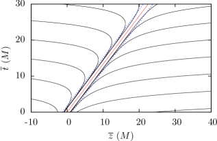
The effect of subtracting the height function from KS time as done in (27) may be visualized by restricting attention to the $\overline{x}=\overline{y}=0$ plane. In that case, (26) reduces to $R=\gamma|\overline{z}-v\,\overline{t}|$ and (27) can be inverted to yield two curves

$$\overline{z} =v\,\overline{t}+\frac{1}{\gamma}\,h_{s}^{-1}(\overline{t}-t),\qquad{\rm for}\qquad\overline{z}>v\,\overline{t},$$ (28a)

$$\overline{z} =v\,\overline{t}-\frac{1}{\gamma}\,h_{s}^{-1}(\overline{t}-t),\qquad{\rm for}\qquad\overline{z}<v\,\overline{t}.$$ (28b)

Fig. 2 shows a set of the resulting nested level-surfaces of trumpet time $t$ plotted in the subspace spanned by KS coordinates $(\overline{t},\overline{z})$. The $t=$ constant surfaces form a foliation that surrounds, but avoids, the moving singularity while still penetrating the horizon.

For a fixed time $\overline{t}$, (26) yields a set of nested ellipsoids centered on $\overline{x}=0$, $\overline{y}=0$, and $\overline{z}=v\overline{t}$. However, once the trumpet time is introduced in (27), for fixed $t$ the ellipsoids diminish in size $R$ as $\overline{t}$ becomes increasingly negative, reaching a limit $R\rightarrow R_{0}$. Effectively the region with KS coordinates such that $R<R_{0}$ is excised from the domain, just as a similar spherical region was excised in the static case. The next step then, also just as in the static case, is to map the (moving) limit surface to a single (moving) point (i.e., puncture) in a way that is consistent with the transformation (13) from Schwarzschild to isotropic coordinates in spherical symmetry.

Figure 2: Cross section of nested level-surfaces of trumpet time $t$ in the $\overline{x}=\overline{y}=0$ plane. The horizontal axis is Kerr-Schild coordinate $\overline{z}$ and the vertical axis is KS time coordinate $\overline{t}$. The trumpet surfaces sweep back in $\overline{t}$ time within the horizon (blue dashed lines), avoiding the singularity (red line) while following its motion.

To make this coordinate transformation, we draw upon the function $R_{s}$ from the static case that follows from solving the differential equations (17) with previously discussed boundary conditions. Here we use $\rho$ as the argument of $R_{s}(\rho)$, which we recall has the properties that $\rho\rightarrow 0$ as $R_{s}\rightarrow R_{0}$ and $\rho/R_{s}(\rho)\rightarrow 1$ as $\rho\rightarrow\infty$. In the static case, $\rho/R_{s}(\rho)$ is the ratio between the new isotropic radial coordinate (there called $r^{\prime}$) and the original Schwarzschild or IEF coordinate $R$. We use this function to define a spatial coordinate transformation

$$x =\overline{x}\frac{\rho}{R_{s}(\rho)},$$

$$y =\overline{y}\frac{\rho}{R_{s}(\rho)},$$ (29)

$$z-vt =\left(\overline{z}-v\overline{t}\right)\frac{\rho}{R_{s}(\rho)},$$

taking $(\overline{x},\overline{y},\overline{z})\rightarrow(x,y,z)$ without making any additional change to the time coordinate $t$ (here $\overline{t}$ is a function of $t$ via (27)). If each equation in (29) is squared and then combined with (26), we find that $\rho$ is related to these new spatial coordinates by

$$\rho^{2}=x^{2}+y^{2}+\gamma^{2}(z-vt)^{2}.$$ (30)

We see that $R=$ constant ellipsoids in KS spatial coordinates, which are limited by $R>R_{0}$ on trumpet slices, map to self-similar $\rho=$ constant ellipsoids in the final spatial coordinates, which are centered on $x=0$, $y=0$, and $z=vt$ and which squeeze the end of the trumpet to that single moving point.

Table 1: Sequence of transformations for boosted trumpet coordinates. The relationship between each system is given to the right of the $\downarrow$.

	Sequence of Coordinate Changes
$\{\overline{t}^{\prime},\overline{x}^{\prime},\overline{y}^{\prime},\overline{z}^{\prime}\}$	Ingoing Eddington-Finkelstein (rectangular)
$\downarrow$	$\overline{t}=\gamma(\overline{t}^{\prime}+v\overline{z})\qquad\overline{z}=\gamma(\overline{z}^{\prime}+v\overline{t})$
$\{\overline{t},\overline{x},\overline{y},\overline{z}\}$	Kerr-Schild (boosted)
$\downarrow$	$t=\overline{t}-h_{s}(R(\overline{t},\overline{x}^{i}))$
$\{t,\overline{x},\overline{y},\overline{z}\}$	(spatial) Kerr-Schild with trumpet slicing
$\downarrow$	$(\overline{x},\overline{y},\overline{z}-v\overline{t})\frac{\rho}{R_{s}(\rho)}=(x,y,z-vt)$
$\{t,x,y,z\}$	Boosted trumpet slice with moving puncture

Summary: Constructing a boosted-trumpet coordinate system for a single black hole involved three consecutive coordinate transformations. The sequence of steps, summarized in Table 1, is (1) a Lorentz boost from IEF to KS, (2) addition of a height function to transform time and introduce the trumpet, and (3) a map to take the trumpet limit surface to the moving puncture.

Combining (24), (27), and (29), we can write the net (reverse) transformation from the final boosted trumpet/puncture coordinates to the initial rectangular IEF coordinates

$$\overline{t}^{\prime} =\gamma^{-1}[t+h_{s}(R_{s}(\rho))]-\gamma v(z-vt)R_{s}(\rho)/\rho,$$ (31a)

$$\overline{x}^{\prime} =xR_{s}(\rho)/\rho,$$ (31b)

$$\overline{y}^{\prime} =yR_{s}(\rho)/\rho,$$ (31c)

$$\overline{z}^{\prime} =\gamma(z-vt)R_{s}(\rho)/\rho.$$ (31d)

In turn, we can write down (in several parts) the line element in the new coordinates

$$ds^{2} =-f{d\overline{t}^{\prime}}^{2}+\left[dx^{2}+dy^{2}+\gamma^{2}(dz-vdt)^{2}\right]\frac{R_{s}^{2}}{\rho^{2}}$$

$$\quad{}+\left(\frac{dR_{s}}{d\rho}-\frac{R_{s}}{\rho}\right)\left(\frac{dR_{s}}{d\rho}+\frac{R_{s}}{\rho}\right)\left(\tensor{\rho}{{}_{,}{}_{a}}\tensor{dx}{{}^{a}}\right)^{2}$$ (32a)

$$\quad{}+\frac{4M}{R_{s}}\frac{dR_{s}}{d\rho}\left(\tensor{\rho}{{}_{,}{}_{a}}\tensor{dx}{{}^{a}}\right)\left[d\overline{t}^{\prime}+\frac{1}{2}\frac{dR_{s}}{d\rho}\left(\tensor{\rho}{{}_{,}{}_{b}}\tensor{dx}{{}^{b}}\right)\right],$$

where the Kerr-Schild coordinate differential $$d\overline{t}^{\prime}$$ above must be replaced with

$$d\overline{t}^{\prime} =\frac{dt}{\gamma}+\frac{1}{\gamma}\frac{dh_{s}}{dR}\frac{dR_{s}}{d\rho}\left(\tensor{\rho}{{}_{,}{}_{a}}\tensor{dx}{{}^{a}}\right)-\gamma v(dz-vdt)\frac{R_{s}}{\rho}$$

$$\qquad{}-\frac{\gamma v(z-vt)}{\rho}\left(\frac{dR_{s}}{d\rho}-\frac{R_{s}}{\rho}\right)\left(\tensor{\rho}{{}_{,}{}_{a}}\tensor{dx}{{}^{a}}\right),$$ (32b)

and where the derivative of (30) gives

$$\tensor{\rho}{{}_{,}{}_{a}}\tensor{dx}{{}^{a}}=\frac{1}{\rho}\left[xdx+ydy+\gamma^{2}(z-vt)(dz-vdt)\right].$$ (32c)

Finally, it is worth asking whether the sequence of steps in Table 1 is essential. For example, it might be possible to use the results of Hannam et al. Hannam et al. (2008) as reviewed in II.1 to construct first an unboosted black hole with trumpet geometry and then apply a global Lorentz boost to the resulting metric in rectangular coordinates. We do not presently know whether this alternative approach might work and it may well be worth future study.

III Setup for Simulations and Numerical Tests

Our simulations were done using the Somerville release of the Einstein Toolkit (ET) ET . A new boosted trumpet initial data thorn was created based on the procedure outlined in the previous section. In addition, we made use of a number of preexisting thorns, including (a modification of) McLachlan McL for evolution and TwoPunctures Ansorg et al. (2004) to generate Bowen-York initial data for comparison simulations as controls (discussed below). Several diagnostic thorns were utilized, including AHFinderDirect Thornburg (1996, 2004) to identify apparent horizons, (a modification of) QuasiLocalMeasures Dreyer et al. (2003) to measure ADM mass and momentum and apparent horizon properties, WeylScal4 Baker et al. (2002) to compute the Weyl curvature quantities, and Multipole Mul to generate spin-weighted spherical harmonic amplitudes of gravitational waveforms. Various results using these thorns are shown in Sec. IV. Post-processing of data was carried out with the help of the SimulationTools package for Mathematica Sim .

To construct the initial data for a single boosted black hole, we start with Mathematica expressions for the components of the metric $\tensor{g}{{}_{a}{}_{b}}$ that produce the line element seen in (32). We then calculate symbolically the first and second derivatives of the metric, $\tensor{g}{{}_{a}{}_{b}{}_{,}{}_{c}}$ and $\tensor{g}{{}_{a}{}_{b}{}_{,}{}_{c}{}_{d}}$. The expressions for the components of the metric and its derivatives are then written to a header file by Mathematica. The lookup table for $dh_{s}/dR$ and $R_{s}$ (and their derivatives) versus $\rho$ is also computed and exported from Mathematica (as described at the end of §II.1.1).

Once the simulation mesh with its refinement levels has been constructed by Carpet, our initial data thorn (written in C) sweeps over the mesh using analytic expressions and interpolations of the numerical solutions for $dh_{s}/dR$ and $R_{s}$ to populate the arrays of required 3+1 quantities. Given a starting time $t$ (typically zero), at every spatial location the code computes $\rho$ based on the specified value of $v$ (and $\gamma$). An interpolation of the lookup table is then made to find $R_{s}(\rho)$ and its first three derivatives and to find $dh_{s}(R_{s}(\rho))/dR$ and its first two derivatives. The interpolation is done with a cubic spline from the Gnu Scientific Library GSL . (The higher derivatives of the numerical functions and the second derivative of the metric are computed in order to assess constraint violations, especially in applications where we superpose two boosted trumpets to initiate a binary encounter.)

At each point interpolated numerical values are inserted in the Mathematica-exported expressions for $\tensor{g}{{}_{a}{}_{b}}$, $\tensor{g}{{}_{a}{}_{b}{}_{,}{}_{c}}$, and $\tensor{g}{{}_{a}{}_{b}{}_{,}{}_{c}{}_{d}}$, and from these we compute the determinants of the full metric ($g$) and spatial metric ($\gamma$), the inverse spatial metric $\tensor{\gamma}{{}^{i}{}^{j}}$, and then the remaining 3+1 quantities

$$\alpha =\sqrt{-g/\gamma},$$ (33a)

$$\tensor{\beta}{{}^{i}} =\tensor{g}{{}_{0}{}_{j}}\tensor{\gamma}{{}^{i}{}^{j}},$$ (33b)

$$\tensor{\beta}{{}^{i}_{,}{}_{t}} =\tensor{g}{{}_{0}{}_{j}{}_{,}{}_{t}}\tensor{\gamma}{{}^{i}{}^{j}}+\tensor{g}{{}_{0}{}_{j}}\tensor{\gamma}{{}^{i}{}^{j}_{,}{}_{t}},$$ (33c)

$$\tensor{K}{{}_{i}{}_{j}} =\frac{1}{2\alpha}\big{[}-\tensor{g}{{}_{i}{}_{j}{}_{,}{}_{0}}+\tensor{g}{{}_{0}{}_{j}{}_{,}{}_{i}}+\tensor{g}{{}_{0}{}_{i}{}_{,}{}_{j}}\big{.}$$

$$\big{.}\qquad\qquad\qquad{}-\tensor{\beta}{{}^{l}}\left(\tensor{g}{{}_{l}{}_{j}{}_{,}{}_{i}}+\tensor{g}{{}_{i}{}_{l}{}_{,}{}_{j}}-\tensor{g}{{}_{i}{}_{j}{}_{,}{}_{l}}\right)\big{]}.$$ (33d)

III.1 Grid Set Up

For a typical boosted black hole simulation, we use Carpet to set up five levels of mesh refinement surrounding the black hole puncture beyond the coarsest adaptive mesh refinement (AMR) level (which covers the entire simulation domain). A baseline grid would have $\Delta x=0.8M$ and $\Delta t=0.36M$ on the coarsest level, with the mesh spacing halved on each successive refinement level. This gives $\Delta x=0.025M$ on the finest level after five refinement steps. On each level the time step is halved also so that the Courant-Friedrichs-Lewy parameter Courant et al. (1928) is maintained. The half-lengths of the AMR cubes are $\{0.9,1.8,3.6,7.2,14.4\}M$ (not including ghost zones). For tests of the effects of resolution, we scale the baseline grid $\Delta x$ and $\Delta t$ down by factors of $2/3$ and $4/9$ and up by a factor $3/2$.

For a single boosted black hole, we also utilize symmetry across $x=0$ and $y=0$ to reduce the computational task. The simulation domain in those cases is $[0,112M]$ along the $x$- and $y$-axes and $[-112M,224M]$ along the $z$-axis. When computing ADM quantities and spin-weighted spherical harmonic projections of Weyl scalars, we integrate over spherical surfaces (as many as four to ten of them) that are centered on the black hole’s original location. These diagnostic surfaces have coordinate radii between $r=33M$ and $r=100M$, spaced evenly in $1/r$.

III.2 Simulation Coordinate Conditions

The numerical evolution uses the 1+log slicing condition

$$\left(\tensor{\partial}{{}_{t}}-\tensor{\beta}{{}^{i}}\tensor{\partial}{{}_{i}}\right)\alpha=-2\alpha K,$$ (34)

(Eq. (7) with $n=2$), which is consistent with the assumption made in our initial data construction. For a static black hole, the advection term in (34) plays a key role in determining both the value of radius $R_{0}$ on the limiting surface of the trumpet and the steady state behavior of the trace of the extrinsic curvature $K$. If the advection term were not included for example, then in steady state ($\partial_{t}\alpha=0$) the slices would become maximal ($K=0$).

An important first test of our initial data and configuration of the evolution code is to see that we recover the known behavior in the static case. Fig. 3 shows our accurate reproduction of a test made in Hannam et al. Hannam et al. (2008) (their Figure 21) in which a static black hole is modeled and the advection term in (34) is turned off (at $t=22.5M$) and turned back on (at $t=72.5M$). During the period when the advection term is switched off, $K$ at the apparent horizon is driven with a damped oscillation to zero. The insets show the relative accuracy maintained in $K$ in the steady state periods before the term is switched off and after it is switched back on. The advection term is utilized under normal circumstances.

Figure 3: Mean curvature $K$ at the apparent horizon of a static black hole versus time. The simulation begins with advection in the 1+log slicing condition turned on. Advection is turned off at $t=22.5M$ and back on again at $t=72.5M$. During the switch-off $K$ is driven from the steady state value $K=6.6856\times 10^{-2}M^{-1}$ toward zero in a damped oscillation over several black hole light crossing times. It accurately recovers (top inset) after advection is switched back on; insets show relative error. The results are consistent with Hannam et al. (2008) (see their Figure 21) and used $\eta=2/M$.

The numerical evolution also uses the hyperbolic $\Gamma$-driver condition Baumgarte and Shapiro (2010) for the shift vector

$$(\tensor{\partial}{{}_{t}}-\tensor{\beta}{{}^{j}}\tensor{\partial}{{}_{j}})\tensor{\beta}{{}^{i}} =\frac{3}{4}\tensor{B}{{}^{i}}$$ (35a)

$$(\tensor{\partial}{{}_{t}}-\tensor{\beta}{{}^{j}}\tensor{\partial}{{}_{j}})\tensor{B}{{}^{i}} =(\tensor{\partial}{{}_{t}}-\tensor{\beta}{{}^{j}}\tensor{\partial}{{}_{j}})\tensor{{\tilde{\Gamma}}}{{}^{i}}-\eta\tensor{B}{{}^{i}}.$$ (35b)

In typical numerical simulations, long term stability is improved by inclusion of the advection terms in this coordinate condition (making it the so-called “shifting shift” condition Baumgarte and Shapiro (2010)). However, the simulation shown in Fig. 3 had the advection terms in the $\Gamma$-driver condition turned off in order to match the conditions used by Hannam et al. Hannam et al. (2008). The parameter $\eta$ also has an effect on stability. Typical values used are $\eta=0$, $\eta=1/M$, or $\eta=2/M$. The previous test was also used to assess the effects of different choices of $\eta$. Fig. 4 shows the response in the coordinate radius of the apparent horizon in the test as the advection term in the 1+log slicing condition is turned off and then back on. When advection is switched off the apparent horizon shrinks in coordinate radius, expelling mesh points from the interior. Once advection is switched back on, the coordinate radius of the apparent horizon grows, seeking to recover its previous value. Two different test simulations are shown, using $\eta=2/M$ and $\eta=0$, with results apparently matching those seen in Figure 22 of Hannam et al. (2008). Coordinate adjustment is faster in the $\eta=0$ case. The results shown in Fig. 3 for changes in $K$ came from the $\eta=2/M$ test simulation.

Figure 4: Coordinate radius of the apparent horizon of a static black hole versus time. The simulation begins with advection in the 1+log slicing condition turned on. Advection is turned off at $t=22.5M$ and back on again at $t=72.5M$. The apparent horizon suddenly shrinks in coordinate radius after $t=22.5M$, only to recover again after advection is restored. Two simulations are shown with $\eta=0$ (solid) and $\eta=2/M$ (dashed).

III.3 Bowen-York Initial Data as a Control

In Sec. IV we examine various consequences of using the new boosted-trumpet initial data in numerical evolutions, making comparisons with the alternative of employing Bowen-York data. For these comparisons Bowen-York initial data are generated by the TwoPunctures thorn Ansorg et al. (2004). Constructing Bowen-York data for a single black hole requires some care however, since TwoPunctures is inherently designed to generate black hole binaries. To obtain a single black hole we first set TwoPunctures to generate a black hole at the center of the mesh with an ADM puncture mass of $M=M_{+}^{ADM}=1$ after having chosen the Bowen-York momentum to be $P_{z}^{+}=\gamma vM$ for a desired $v$. Next, a second black hole with ADM puncture mass of $M_{-}^{ADM}=10^{-4}M$ and momentum $P_{z}^{-}=0$ is specified at a distance of $d=2\,000M$ from the origin. Once TwoPunctures maps its solution to the actual computational domain, we end up with data for a single moving Bowen-York black hole superposed with a slight tidal field contribution that is below the level of truncation error ($M^{\textrm{ADM}}_{-}/d^{3}\simeq 10^{-14}M^{-2}$).

We can assess the accuracy in specifying initial data by either means by examining the degree of violation of the Hamiltonian constraint

$$H=R+K^{2}-K_{ij}K^{ij}=0.$$ (36)

In Fig. 5 we show the Hamiltonian constraint violation in the initial data by plotting $\log(|H|)$ along the $z$-axis. Since the boosted-trumpet initial data for a single hole is derived from a partly-analytic, partly-numerical coordinate transformation of the Schwarzschild metric, it suffers very small Hamiltonian constraint violations over most of the mesh. The larger Hamiltonian constraint violations in the Bowen-York data result from the level of convergence attained within the TwoPunctures routine. As is well known, the constraint violation rises sharply near the puncture (see figure inset), due in part to difficulty in computing accurate finite differences of spatial curvature at that location. These large deviations from the constraint are enclosed within the horizon. The near-puncture violations of the Hamiltonian constraint are larger in the Bowen-York case, due again to (discretionary) limits set on convergence within TwoPunctures.

Figure 5: Violations of the Hamiltonian constraint. The violation is shown by plotting $|H|$ along the $z$-axis in both the boosted-trumpet (black) and Bowen-York (red) initial data. In each case the black hole was given $v=0.5$ in the positive $z$ direction. Large violations of the constraint near the puncture are confined within the horizon.

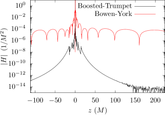
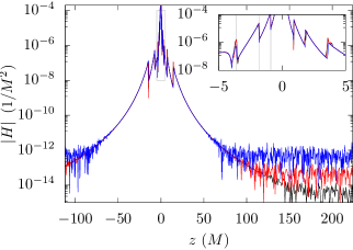
The mesh resolution dependence of the Hamiltonian constraint violation in the boosted-trumpet initial data is shown in Fig. 6. In principle, a metric derived from a coordinate transformation of a Schwarzschild black hole should satisfy the constraints exactly. The small levels of error seen here are primarily due to finite difference errors in computing the spatial curvature. As such, the errors improve with increasing resolution. This is demonstrated in the plot by scaling the errors under the assumption of fourth-order convergence. The black curve corresponds to the standard grid spacing $\Delta x=0.8M$ on the coarsest level and the errors are not scaled. The red and blue curves come from simulations which have grid spacings scaled down by $\frac{2}{3}$ and $\frac{4}{9}$, respectively; to demonstrate convergence their errors are scaled by the relevant mesh ratio to the inverse fourth power. The boundaries of the AMR regions are visible, especially in the inset, caused by discontinuous changes in grid spacing.

Figure 6: Hamiltonian constraint violation scaled to show fourth order convergence. Plotted is $|H|$ along the $z$-axis for boosted-trumpet initial data at three resolutions. The black curve has default grid spacing $\Delta x=0.8M$ on the coarsest level. The red and blue curves have grid spacings scaled down by $\frac{2}{3}$ and $\frac{4}{9}$, respectively. Fourth order convergence is demonstrated by multiplying the medium resolution curve by $(3/2)^{4}$ and the high resolution curve by $(9/4)^{4}$ so that they are coincident with the low resolution curve. The black hole was set to have $v=0.5$ in the positive $z$ direction. In the inset the locations of some AMR boundaries are indicated by vertical gray lines.

IV Results

IV.1 Qualitative Description of Boosted-Trumpet Data at $t=0$ and After Evolution

We begin the consideration of numerical evolution of the boosted-trumpet initial data with a plot of several 3+1 quantities in a planar cross section of the mesh. A primary motivation for constructing initial data on a trumpet slice from the outset was the expectation that the initial data would be “closer” to the steady state of the moving punctures gauge conditions than, for example, Bowen-York data. Fig. 7 shows this expectation to be borne out. The plot makes a side by side comparison of a boosted-trumpet simulation (left side) and a Bowen-York simulation (right side), showing $t=0$ in the two top panels and $t=198M$ in the bottom two panels. Each figure is a section of the $x$,$z$ plane, centered on the instantaneous position of the black hole. Displayed within each figure are (solid black) contours of the lapse, arrows showing the $x$,$z$ components of the shift vector, the trapped region (blue shaded) within the apparent horizon, and a red dot showing the puncture location. The (red) boxes show AMR boundaries. In both cases the black hole parameters are set to give it an eventual steady-state velocity of $v=0.5$ in the positive $z$-direction.

Figure 7: Boosted-trumpet versus Bowen-York simulations. Snapshots at $t=0$ (top panels) and at $t=198M$ (bottom panels) are shown. The left panels depict the boosted-trumpet simulation while those on the right show the Bowen-York comparison. Snapshots are a segment of the $x$,$z$ plane centered on the black hole and show (solid black) contours of the lapse, $x$ and $z$ components of the shift vector, trapped region (blue shaded) within the apparent horizon, and puncture location (red dot). AMR boundaries are also shown (red box). At $t=0$ the Bowen-York shift identically vanishes. Lapse contours are spaced by $0.1$ with a couple of values labeled. Each snapshot has equivalent spatial scale, though at late time are centered on different locations. Each simulation had eventual steady-state black hole velocity of $v=0.5$, but the Bowen-York hole had to accelerate from $v=0$ initially (see Fig. 15). Simulations used $\eta=0$.

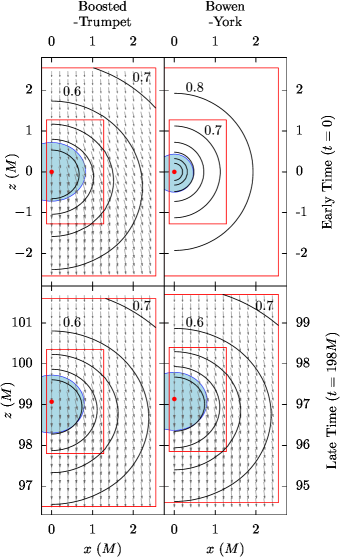
At late times ($t\simeq 198M$) the metric near the black hole is very similar in the two simulations, except the Bowen-York hole has not advanced as far in coordinate distance. This is due in part to the Bowen-York hole having a vanishing shift vector $\tensor{\beta}{{}^{i}}$ initially (Fig. 7, upper right), and hence a vanishing initial puncture velocity. The shift vector in the boosted-trumpet initial data is nonvanishing, and bears considerable resemblance to the steady-state shift at late time in the same simulation. The coordinate size of the apparent horizon in the Bowen-York initial data is smaller than its eventual steady-state dimensions. There is much less change during the simulation in the coordinate size of the apparent horizon in the boosted-trumpet case.

IV.2 Quasi-local Energy and Momentum

A primary reason for introducing trumpet slicing for initial data is to be able to better specify black hole momentum than is otherwise possible with Bowen-York data. Momentum and energy of initial data can be determined in numerical relativity calculations using quasi-local measures of ADM momentum and ADM energy Baumgarte and Shapiro (2010). Within the Einstein Toolkit there exists a routine QuasiLocalMeasures Dreyer et al. (2003) for computing these estimates of the asymptotic quantities on two-surfaces of specified radius. The ADM energy and momentum of Bowen-York black holes was studied previously York and Piran (1982); Cook and York (1990). The conformally-flat nature of that data leads to the presence of spurious gravitational radiation, which adds to the ADM energy and affects the ability to specify the velocity (or Lorentz factor) of the black hole Cook and York (1990); Sperhake et al. (2008).

To make the analogous study of energy and momentum of boosted-trumpet initial data, we sought to make sharp estimates of (asymptotic) ADM energy and momentum by extrapolating the quasi-local measures. To this end, we found it convenient to write somewhat simpler quasi-local energy and momentum integrals than are found in QuasiLocalMeasures. We use

$$E_{\textrm{ADM}}(r)=\frac{1}{16\pi}\oint_{r}\left[\tensor{\delta}{{}^{i}{}^{j}}\tensor{h}{{}_{k}{}_{j}{}_{,}{}_{i}}-\tensor{\partial}{{}_{k}}\left(\tensor{\delta}{{}^{i}{}^{j}}\tensor{h}{{}_{i}{}_{j}}\right)\right]\frac{\tensor{x}{{}^{k}}}{r}r^{2}d\Omega,$$ (37)

and

$$\tensor{{P_{\textrm{ADM}}}}{{}^{i}}(r)=\frac{1}{8\pi}\oint_{r}\tensor{\delta}{{}^{k}{}^{i}}\bigg{[}\frac{1}{2}\left(\tensor{h}{{}_{k}{}_{0}{}_{,}{}_{j}}+\tensor{h}{{}_{j}{}_{0}{}_{,}{}_{k}}-\tensor{h}{{}_{j}{}_{k}{}_{,}{}_{t}}\right)\bigg{.}$$

$$\qquad\qquad\qquad\bigg{.}-\tensor{\delta}{{}_{k}{}_{j}}\left(\tensor{h}{{}_{l}{}_{0}{}_{,}{}_{l}}-\frac{1}{2}\tensor{h}{{}_{l}{}_{l}{}_{,}{}_{t}}\right)\bigg{]}\frac{\tensor{x}{{}^{j}}}{r}r^{2}d\Omega,$$ (38)

where $\tensor{h}{{}_{i}{}_{j}}\equiv\tensor{g}{{}_{i}{}_{j}}-\tensor{\delta}{{}_{i}{}_{j}}$. In the limit $r\rightarrow\infty$ these expressions yield the ADM quantities: $E_{\textrm{ADM}}=E_{\textrm{ADM}}(\infty)$ and $\tensor{{P_{\textrm{ADM}}}}{{}^{i}}=\tensor{{P_{\textrm{ADM}}}}{{}^{i}}(\infty)$. These particular quasi-local formulae match those discussed in Alcubierre (2008) and we wrote a modified version of QuasiLocalMeasures for their use.

By inserting the boosted-trumpet metric (32) with the expansions from §II.1.2 into (37) and (38), and having Mathematica perform series expansions and integrals at $t=0$, we obtained asymptotic expansions for the ADM energy and momentum

$$E_{\textrm{ADM}}(r) \simeq\gamma M+e_{1}(\gamma)\frac{M^{2}}{r}+e_{2}(\gamma)\frac{M^{3}}{r^{2}}+e_{3}(\gamma)\frac{M^{4}}{r^{3}},$$ (39)

$$P_{\textrm{ADM}}(r) \simeq\gamma vM+p_{1}(\gamma)\frac{M^{2}}{r}+p_{2}(\gamma)\frac{M^{3}}{r^{2}}+p_{3}(\gamma)\frac{M^{4}}{r^{3}},$$ (40)

out to the indicated order. Here the coefficients in the expansions are somewhat complicated expressions of $\gamma$ (or $v$), which for brevity we leave off listing. It is apparent that asymptotically the initial data preserve the expected Christodoulou Christodoulou (1970) energy-momentum relation $E_{\textrm{ADM}}^{2}=P_{\textrm{ADM}}^{2}+M^{2}$. We also treated the coefficients as unknowns, measuring $E_{\textrm{ADM}}(r)$ and $P_{\textrm{ADM}}(r)$ at a minimum of four radii, and made fits to the expansions to cubic order in $1/r$. Comparison between the numerically determined coefficients and their expected analytic values provided a strong check on the quasi-local measures, and the intercepts (at infinity) provided sharp, extrapolated estimates of energy and momentum. Making this direct comparison is what necessitated introducing the modified versions of the ADM quantities (37) and (38).

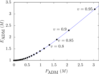
The result of extracting the extrapolated estimates for boosted-trumpet data is shown in Fig. 8. The extrapolated values of $E_{\textrm{ADM}}$ and $P_{\textrm{ADM}}$ are shown plotted against each other as a set of points for different prescribed boost parameters (with the last few points being marked by their associated velocity parameter). These data are well fit (blue curve) by the expected hyperbolic relationship between $E_{\textrm{ADM}}$, $P_{\textrm{ADM}}$, and $M$. Comparison can be made to the Bowen-York case Cook and York (1990) (Figure 1 in that paper) where increasing (junk) gravitational radiation limited the range of specifiable black hole velocity.

Figure 8: ADM energy versus ADM momentum for boosted-trumpet initial data. Boosted-trumpet black hole initial data were computed for a set of velocities up to $v_{\textrm{max}}=0.95$. Quasi-local estimates of ADM energy and momentum were computed on a set of two-surfaces with radii from $r=33M$ to $r=100M$. Asymptotic expansions of energy and momentum were fit to determine estimates of ADM energy and momentum at spacelike infinity. The resulting values are shown plotted against each other (black dots). The blue curve displays the expected Christodoulou relationship $E_{\textrm{ADM}}^{2}=P_{\textrm{ADM}}^{2}+M^{2}$ for a boosted black hole.

IV.3 Reduced Junk Gravitational Radiation

Another primary motivation in developing boosted-trumpet initial data is to reduce or eliminate junk radiation. Curvature in vacuum is characterized by the Newman-Penrose (or Weyl) scalars $\psi_{0},\ldots,\psi_{4}$, defined by contracting the Weyl tensor on a suitable null tetrad. When a quasi-Kinnersley tetrad $(l,k,m,\overline{m})$ is selected, the scalars $\psi_{0}$ and $\psi_{4}$ primarily measure ingoing and outgoing gravitational radiation, respectively, while $\psi_{2}$ represents the “Coulombic” part of the field. To extract gravitational waves, we focus on $\psi_{4}$, which is defined by

$$\psi_{4}=\tensor{C}{{}_{a}{}_{b}{}_{c}{}_{d}}\tensor{k}{{}^{a}}\tensor{{\overline{m}}}{{}^{b}}\tensor{k}{{}^{c}}\tensor{{\overline{m}}}{{}^{d}},$$ (41)

where $\tensor{k}{{}^{a}}$ is the radially ingoing null vector and $\tensor{{\overline{m}}}{{}^{a}}$ is a complex angular null vector. Then at sufficient distance from the source, the two metric perturbation polarizations (waveforms) are determined by the real and imaginary parts of $\psi_{4}$:

$$\psi_{4}=\ddot{h}_{+}-i\ddot{h}_{\times}.$$ (42)

Drawing upon the Einstein Toolkit we use the routines WeylScal4 and Multipole to compute $\psi_{4}$ and extract from it its $s=-2$ spin-weighted spherical harmonic amplitudes as functions of time at fixed radii. In WeylScal4 the quasi-Kinnersley tetrad is obtained Baker et al. (2002) using the full (simulation) metric, with the radial and angular directions defined relative to the center of the mesh.

Figure 9: Gravitational waveform from single boosted-trumpet black hole and underlying background. Shown is the $l=2$, $m=0$ amplitude (black curve) of $\psi_{4}$ evaluated at a coordinate radius of $100M$. The junk waveform lies primarily in the interval $t=80-140M$. Light dotted, dashed, and solid curves show successive approximations [given by (44)] to the underlying, nonradiative background in this signal (see text). Simulation used $\eta=1/M$.

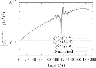
We use these tools to measure the junk gravitational radiation content of our boosted-trumpet initial data. Given axisymmetry, the $l=2$, $m=0$ mode dominates the radiation. Fig. 9 displays this amplitude (black curve) extracted at $r=100M$ as a function of $t$ from a simulation of a single black hole specified to have $v=0.5$. The time series contains two components, with the high frequency signal in the interval $t=80-140M$ being the junk radiation. The high frequency waveform peaks at $t\simeq 110M$, with the time delay indicating that the junk emerges from the region very near the black hole. The size of this pulse of junk radiation is sufficiently small (to be established shortly) that the curve is dominated by a second component–a smooth underlying background whose source we discuss next.

IV.3.1 Effects of Offset Tetrad

In the rest frame of a Schwarzschild black hole and in the naturally associated Kinnersley tetrad $(l^{\prime},k^{\prime},m^{\prime},\overline{m}^{\prime})$, all of the Weyl scalars vanish except $\psi^{\prime}_{2}=-M/R^{3}$. Any radiation added as a perturbation would appear in $\psi^{\prime}_{4}$ and $\psi^{\prime}_{0}$. When a boosted black hole is modeled two things affect this clean separation. First, the tetrad constructed by WeylScal4 $(l,k,m,\overline{m})$ will be in a frame boosted with respect to the static-frame tetrad. Even at $t=0$ the frame components differ (e.g., (25)) and the new frame components are linear combinations of those in the static frame. Second, a single black hole does not remain centered on the mesh origin, so the linear transformation between frames is time dependent and as time proceeds the tetrad generated by the code rapidly ceases to reflect the principal null directions of the black hole. The net effect is that the $\psi_{4}$ measured by the code will itself be a linear combination of Weyl scalars in the static frame

$$\psi_{4}={A_{(4)}}^{(4)}\psi^{\prime}_{4}+{A_{(4)}}^{(2)}\psi^{\prime}_{2}+{A_{(4)}}^{(0)}\psi^{\prime}_{0},$$ (43)

and will reflect a time-dependent mixing with the longitudinal field.

To confirm that the underlying trend in Fig. 9 is due to frame mis-centering and not radiation, we can take the initial data metric (32) for a boosted black hole, with its full time dependence, construct the curvature tensor, and then project the curvature on a tetrad constructed exactly as done in WeylScal4. The initial data metric is exactly a Schwarzschild black hole, just in boosted trumpet coordinates, so it would have vanishing Weyl scalars in the Kinnersley frame except $\psi^{\prime}_{2}$ (i.e., no radiation). In the mesh-centered frame, however, we find $\psi_{4}\neq 0$. To compute this comparison we made an asymptotic expansion of the metric (32), using in part the expansions for $h_{s}(R)$ and $R_{s}(\rho)$ from §II.1.2, to obtain expansions of $\psi_{4}$. That expansion was in turn projected on the $s=-2$ spin-weighted spherical harmonics, allowing us to extract the $l=2,m=0$ amplitude as an expansion in $1/r$ and as a function of time. The calculation was done in Mathematica and yielded a complicated expression in terms of $v,M,r,t$. Setting $v=0.5$ for the case considered in Fig. 9, we find

$$\psi_{4}^{(2,0)}\left(v=\tfrac{1}{2}\right)=-\sqrt{\frac{5\pi}{2}}\frac{M}{4r^{3}}\left(27\ln 3-28\right)$$

$$\quad{}-\sqrt{\frac{5\pi}{2}}\frac{M}{24r^{4}}\Big{[}\left(225\sqrt{3}-142\pi\right)M+12\left(27\ln 3-28\right)t\Big{]}$$

$$\quad{}-\sqrt{\frac{5\pi}{2}}\frac{M}{1512r^{5}}\Big{[}4\left(4493-960\sqrt{3}\right)M^{2}\Big{.}$$

$$\qquad\Big{.}{}+126\left(130\pi-261\sqrt{3}\right)Mt+378\left(27\ln 3-28\right)t^{2}\Big{]}$$

$$\quad{}+\mathcal{O}(r^{-6}).$$ (44)

It is clear that the claimed mixing occurs, even at $t=0$, and is made worse as the black hole shifts toward the extraction radius $r$.

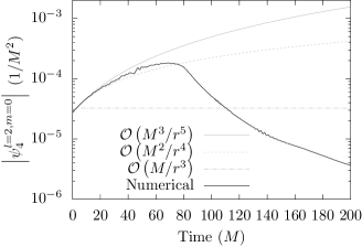
In Fig. 9 we show the progressive influence of terms in the expansion (44), starting with the (constant) $M/r^{3}$ (dotted) term and adding in the $M^{2}/r^{4}$ (dashed) and $M^{3}/r^{5}$ (solid) terms. Successive terms better approximate the smooth underlying trend. However, our approximate analysis breaks down at late times, as can be seen in Fig. 10, once the black hole drifts into contact with and moves beyond the extraction radius and our asymptotic expansions are no longer valid. The conclusion remains, though, that the junk radiation is the smaller high-frequency signal superimposed on the smooth non-radiative underlying trend. The junk radiation is clearly seen in Fig. 9, where the extraction radius is $r=100M$, but is barely noticeable in Fig. 10, where $r=33M$ and the $r^{-3}$ longitudinal term dominates the $r^{-1}$ radiative term.

Figure 10: Gravitational waveform from single boosted-trumpet black hole and underlying background. Shown is the $l=2$, $m=0$ amplitude (black curve) of $\psi_{4}$ evaluated at a coordinate radius of $33M$. The (small) junk waveform lies in the interval $t=25-50M$. Light dotted, dashed, and solid curves show successive approximations [given by (44)] to the underlying, nonradiative background (see text). The approximate explanation of this background breaks down beyond $t\simeq 66M$, as discussed in the text. Simulation used $\eta=1/M$.

IV.3.2 Boosted-Trumpet versus Bowen-York Junk Radiation

Our method of constructing boosted-trumpet initial data greatly minimizes junk radiation, and its resulting small amplitude is the reason the radiation is dominated by the offset-tetrad effects in the preceding two plots. To quantify this claim we ran a comparison simulation with Bowen-York initial data and with exactly the same prescribed black hole momentum. The $l=2,m=0$ amplitude of $\psi_{4}$ was extracted similarly at $r=100M$ and $r=33M$ and overlaid on the comparison boosted-trumpet waveform at the same radii.

Figure 11: Junk radiation comparison between simulations with boosted-trumpet and Bowen-York initial data. The dominant $l=2,m=0$ amplitude of the Weyl scalar $\psi_{4}$ is extracted at $r=100M$ in a boosted-trumpet simulation (black curve) and Bowen-York comparison (red curve). Following passage of the pulse the waveforms match, reflecting the nonradiative offset-tetrad background. Simulations used $\eta=1/M$.

Figure 12: Junk radiation comparison between simulations with boosted-trumpet and Bowen-York initial data. Same as Fig. 11 except on a linear scale. Bowen-York signal (red curve) dominates over the barely visible wave (black curve) from the boosted-trumpet model.

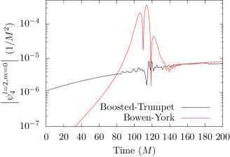
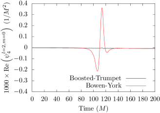
Fig. 11 shows the $l=2$, $m=0$ amplitude of $\psi_{4}$ as a function of time extracted at $r=100M$ for both the $v=0.5$ boosted-trumpet black hole simulation (black curve) and the comparable Bowen-York model (red curve). The Bowen-York junk radiation pulse centered about $t\simeq 110M$ has an amplitude nearly two orders of magnitude larger than the boosted-trumpet pulse. After the passage of the pulse, the waveform settles in both simulations to the nonradiative offset-tetrad background. At early times, before the arrival of the pulse, the asymptotic behavior of the Bowen-York data differs from boosted-trumpet dependence, rendering our offset-tetrad analysis inapplicable until passage of the junk pulse. Fig. 12 shows the same comparison but on a linear scale, making even more evident the drastic reduction in junk radiation amplitude.

Figure 13: Junk radiation comparison between simulations with boosted-trumpet and Bowen-York initial data. Same as Fig. 11 except the waveforms are extracted at a radius of $33M$. At late times following passage of the pulse, the nonradiative offset-tetrad background prevails, with a relative delay evident in the arrival of the Bowen-York black hole at the extraction radius due to early coordinate velocity changes. Simulations used $\eta=1/M$.

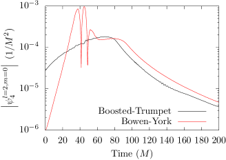
Fig. 13 shows the same comparison between $l=2,m=0$ amplitudes of $\psi_{4}$ but extracted at $r=33M$. It is still clear that the Bowen-York junk pulse is several orders of magnitude larger than the boosted-trumpet pulse, though the offset-tetrad effects are more pronounced at this radius. At late times after the passage of the junk pulse, the two waveforms behave similarly. The relative delay in the Bowen-York signal can be ascribed to a coordinate effect, as the Bowen-York black hole is delayed in reaching the extraction radius by about $10M$ (in the $\eta=1/M$ simulation) because it must accelerate from vanishing initial velocity.

Finally, there is the matter of what sets the scale of junk radiation in the boosted-trumpet case and why it is present at all. In principle our prescription for a single boosted-trumpet black hole is merely a coordinate transformation of the exact Schwarzschild spacetime, which contains no radiation whatsoever, and the adjustment to moving-punctures gauge is a coordinate effect. This certainly explains why the boosted-trumpet junk is orders of magnitude smaller than that associated with Bowen-York data. The fact that the boosted-trumpet junk radiation is not exactly zero can be ascribed to numerical errors in constructing the initial data. For example, we make numerical approximations for $dh_{s}/dR$ and $R_{s}$, and these approximations enter into the initial metric (32) in several places. Additionally, components of the metric (32) are sampled at the mesh points and then other quantities, including finite differences for derivatives, are computed via (33) to round out the initial data. These numerical steps leave in their wake discretization and finite-difference errors.

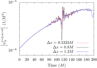
What are the effects of changing mesh resolution? Fig. 14 shows the waveform extracted at $r=100M$ for simulations with three different mesh resolutions. The early part of the waveform due to the offset-tetrad effects is nearly insensitive to changes in resolution, indicating a nonvanishing and fairly well-resolved behavior. The higher frequency junk signal, on the other hand, is sensitive to changes in resolution without exhibiting a clear power-law scaling that would be expected of finite differencing a smooth function. That lack of scaling likely stems from one or more sources. First, as we scaled the computational mesh we did not also simultaneously scale the resolution on the spherical surfaces upon which the angular harmonic parts of $\psi_{4}$ are computed. Second, we also did not simultaneously scale the resolution of the lookup table. Third, by construction, the junk radiation in our scheme should vanish analytically, which means that a numerical computation of $\psi_{4}$ will be subject to roundoff errors as projecting the Weyl tensor involves differencing nearly identical terms. Finally, the small errors in the lookup table can show up in the boosted-trumpet metric in a stochastic fashion, since the tabulated spherical functions are sampled onto a rectangular grid.

Figure 14: Resolution dependence of the boosted-trumpet junk radiation and the offset-tetrad background waveform. The same $l=2$, $m=0$ amplitude of $\psi_{4}$, extracted at $r=100M$, is shown for three simulations with mesh resolutions indicated on the plot. The early offset-tetrad effect is well-resolved, while the junk radiation signal is highly sensitive to changes in resolution, indicative of discretization and sampling errors. Simulations used $\eta=1/M$.

IV.4 Coordinate Velocity of the Black Hole

The Bowen-York prescription determines $g_{ij}$ and $K_{ij}$ within the initial spacelike slice but leaves unspecified the lapse $\alpha$ and shift $\beta_{i}$ both on and in the future of the initial surface. Lacking any better choice the initial shift is frequently set to zero. When used in a moving-punctures simulation, the mesh points near the Bowen-York center (other end of the wormhole) rapidly draw toward the trumpet surface and become points near the puncture (limit surface of the trumpet) Hannam et al. (2008). One measure of the motion of the black hole is (minus) the value of the shift at the puncture. As is well known, this has the odd, though purely coordinate, effect that in a Bowen-York simulation a black hole with initial linear momentum has no initial velocity. We saw the effect in coordinate position/time delays both in Fig. 7 and in Fig. 13.

In our boosted-trumpet procedure the full spacetime metric is constructed initially, which means that starting conditions for the lapse and (nonzero) shift are given. Given the initial value of the shift at the puncture, the velocity of the black hole (as determined by the shift) will be specified correctly, consistent with the expected stationary value. In practice, the puncture velocity varies in time somewhat, over a few light crossing times up to hundreds of $M$ depending upon $\eta$, before settling back to its original value.

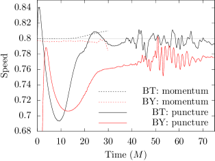
Fig. 15 shows black-hole coordinate speed as determined by the shift at the puncture for several boosted-trumpet and Bowen-York simulations, all with parameters set for steady state velocity $v=0.5$. In the boosted-trumpet simulation (solid black curve) made with $\eta=0$, the black hole’s speed is very stable and settles to its specified value as the coordinates relax over a few light crossing times. In the comparable Bowen-York simulation (solid red) the black hole abruptly accelerates and reaches its stationary coordinate speed in just slightly longer time. The velocity profile of the Bowen-York black hole is primarily due to the initially vanishing shift, as can be seen by a third simulation (solid blue) where we set the initial boosted-trumpet shift to zero. The $\eta$ parameter in the $\Gamma$-driver condition plays a large role in the evolution of the black hole velocity. The three simulations just described (with $\eta=0$) were repeated (dotted curves) after changing to $\eta=1/M$. Black hole coordinate velocity (as measured by the shift at the puncture) reaches its asymptotic value much more rapidly when $\eta=0$. This is consistent with the behavior in Fig. 4 where the apparent horizon radius recovers from gauge changes more rapidly when $\eta=0$.

Figure 15: Black hole speed computed from puncture value of shift versus time. Each simulation was initiated to have momentum consistent with $v=0.5$. Solid curves depict simulations with $\eta=0$. BT denotes boosted-trumpet simulations, while BY corresponds to Bowen-York models. The blue solid curve shows a boosted-trumpet model with $\beta_{i}=0$ initially. Dotted curves correspond to the same simulations but with the gauge condition set to $\eta=1/M$.

Figure 16: Puncture velocity for boosted-trumpet black holes versus time for various specified speeds. Specified initial and asymptotic speeds are indicated by the light horizontal lines. Readjustment of the trumpet shape and settling of the spatial coordinates occur during $t\lesssim 25M$. Simulations used $\eta=0$.

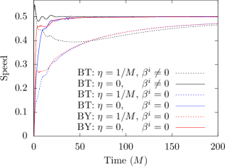
Fig. 16 shows the black hole puncture-velocity history for a set of boosted-trumpet simulations with increasing Lorentz boosts. Settling of the coordinates primarily occurs within the first $25M$ in time as the black hole coordinate velocities tend toward their specified values (light horizontal lines). The highest velocity model corresponds to Lorentz factor $\gamma=1.90$. Beyond this boost, we encountered problems with stability. The instability might result from the true steady-state trumpet being too distorted relative to our initially assumed spherically symmetric trumpet. Alternatively, we may merely need more mesh resolution at Lorentz factors $\gamma>1.9$ than we were able to employ in this study.

A closer comparison between boosted-trumpet and Bowen-York black holes at high Lorentz factor can be seen in Fig. 17. The boosted-trumpet black hole (black curves) was specified by directly setting the boost velocity parameter to be $v=0.8$, or equivalently setting $\gamma=1.667$. The Bowen-York simulation was initialized by requiring the ADM mass at the puncture be $M=1$ and setting the Bowen-York momentum parameter to be $P=\gamma v=1.333$. Once the simulations are begun, we monitor the apparent horizon mass (a close proxy for the irreducible mass $M_{irr}$) and the (extrapolated to infinity) ADM momentum $P_{\rm ADM}$. The latter two measures are then combined to yield an asymptotically-sensed estimate of the Lorentz factor,

$$\gamma=\sqrt{1+\left(\frac{P_{\textrm{ADM}}}{M_{\textrm{irr}}}\right)^{2}},$$ (45)

and from that the velocity $v$. This estimate of the velocity is plotted in Fig. 17 (dotted curves) at early times ($t<30M$) for both the boosted-trumpet (black) and Bowen-York (red) cases. (By $t=30M$ and later the combination of outward-moving junk radiation and drift of the black hole toward the inner extraction radius makes extrapolated estimates of $P_{\rm ADM}$ unreliable.) In the boosted-trumpet case, this measure of $v$ is indistinguishable at the resolution of the plot from the parameter choice in the initial data. In the Bowen-York case, the asymptotic estimate of $v$ is a few thousandths smaller than the prescribed velocity, primarily because of the difference between the initial value parameter $M=1$ and the actual values of $M_{irr}$.

As an alternative, we plot in Fig. 17 the puncture velocity of the black holes (solid curves) extracted from the two comparison simulations. Once transient gauge effects have decayed the boosted-trumpet puncture velocity averages close to $v=0.8$ (solid black curve). The late-time puncture velocity in the Bowen-York case averages about $v=0.78$ (solid red curve). When converted to energy, this deficit corresponds to the Bowen-York black hole having about 4% less energy than the boosted-trumpet hole, a drop ascribable to momentum and energy carried off by junk radiation and consistent with the undesired renormalization of initial momentum seen previously Sperhake et al. (2008) when using the Bowen-York prescription.

Figure 17: Measures of black hole velocity at prescribed Lorentz factor $\gamma=1.667$ ($v=0.8$). Black curves correspond to the boosted-trumpet case and red curves to the Bowen-York. Dotted curves estimate the velocity at early times using ADM momentum [see (45)]. Solid curves show black hole velocity measured by the shift vector at the puncture. Simulations used $\eta=0$.

IV.5 Apparent Horizon Comparisons

We made further comparisons between boosted-trumpet and Bowen-York simulations by looking at circumferences on the apparent horizon. Using AHFinderDirect first to locate the apparent horizon as a function of time and then using QuasiLocalMeasures, we computed the (maximum) proper circumferences of the apparent horizon in the $xy$-, $xz$-, and $yz$-planes

$$C_{xy} =\int^{2\pi}_{0}d\phi\sqrt{\tensor{q}{{}_{\phi}{}_{\phi}}\left(\theta=\pi/2,\phi\right)}$$ (46a)

$$C_{xz} =2\int^{\pi}_{0}d\theta\sqrt{\tensor{q}{{}_{\theta}{}_{\theta}}\left(\theta,\phi=0\right)}$$ (46b)

$$C_{yz} =2\int^{\pi}_{0}d\theta\sqrt{\tensor{q}{{}_{\theta}{}_{\theta}}\left(\theta,\phi=\pi/2\right)}.$$ (46c)

Here $\tensor{q}{{}_{A}{}_{B}}$ is the 2-metric on the apparent horizon

$$\tensor{q}{{}_{A}{}_{B}}=\frac{\partial\tensor{x}{{}^{i}}}{\partial\tensor{\theta}{{}^{A}}}\frac{\partial\tensor{x}{{}^{j}}}{\partial\tensor{\theta}{{}^{B}}}\tensor{g}{{}_{i}{}_{j}},$$ (47)

where $A,B\in\{\theta,\phi\}$. Just like the apparent horizon, these proper lengths are not gauge invariant but depend upon the slicing condition. For a Schwarzschild black hole in static coordinates these circumferences would all be equal, so any ratio would be unity.

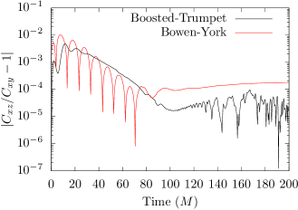
In Fig. 18 we plot the absolute value of the difference between the aspect ratio $C_{xz}/C_{xy}$ and unity on a log scale for simulations of $v=0.5$ black holes. In the Bowen-York case (red curve) there is an initial distortion at about the 1% level that subsequently decays by two orders of magnitude in a damped oscillatory motion. This oblate to prolate oscillation suggests excitation of black hole quasinormal ringing, excited by the junk radiation, though with the ringing sensed locally in the apparent horizon properties and not remotely in the gravitational waveform. In contrast, in the boosted-trumpet case (black curve) there is an initial distortion followed by rapid decay, but one lacking in repeated oscillations about zero. In this case the significantly decreased presence of junk radiation bars noticeable quasinormal excitation of the apparent horizon. A distortion is still present, because of the inconsistency between our initial trumpet shape and the steady state trumpet that emerges at late times in moving-punctures gauge, which decays as the time slices adjust.

Figure 18: Ratios of circumferences of the apparent horizon as functions of simulation time. Both boosted-trumpet (black) and Bowen-York (red) black holes are set for $v=0.5$. The damped oscillation in the Bowen-York case is suggestive of excitation of quasinormal ringing caused by the junk radiation. The boosted-trumpet distortion likely arises from evolution in the time slices as the trumpet shape and coordinates adjust. Simulations used $\eta=1/M$.

V Conclusions

We have demonstrated a means of constructing boosted-trumpet initial data for single black holes for use in moving-punctures simulations. The procedure uses (1) a global Lorentz boost applied to Kerr-Schild coordinates, followed by (2) changing the time slice to trumpet topology by adding an appropriate height function, and (3) changing spatial coordinates to map the trumpet limit surface to a single (moving) point (i.e., the puncture). This method can be extended to widely separated multiple black holes by superposing initial data; it could also form the basis for a prescription for specifying initial data for closer binaries as the initial guess for a re-solving of the constraint equations.

We showed in simulations that the boosted-trumpet initial data more closely approximates eventual steady state geometry than does Bowen-York initial data. Asymptotic ADM energy and momentum and apparent horizon mass follow closely the Christodoulou relationship, allowing large black hole velocities to be assigned (tested as high as $v=0.95$).

Gravitational junk radiation is suppressed in simulations using the new scheme by two orders of magnitude relative to simulations with Bowen-York data of comparable parameters. The essential element in reducing the junk radiation was use of non-conformally-flat boosted Kerr-Schild geometry as an intermediate step in constructing the new data, with a trumpet introduced to ensure that the slice avoids the future singularity. What junk radiation remains in the boosted-trumpet case is sensitive to changes in mesh resolution, reflecting an origin in sampling numerical data from a lookup table and resulting discretization errors. Black holes initiated with the boosted-trumpet scheme have nonzero initial puncture velocities consistent with the intended boost. As simulations begin, the puncture velocity varies for several black hole light crossing times before settling back to the intended value. In the Bowen-York case, the eventual average puncture velocity is reduced slightly relative to the initial parameter value, reflective of some energy and momentum carried off in the junk radiation. We also studied changes in the proper circumferences of the apparent horizon as functions of time. The shape of the apparent horizon in the Bowen-York simulations suffers a damped oscillatory motion, suggestive of excitation of black hole quasinormal modes. In contrast there is no noticeable ringing in the aspect ratio of the apparent horizon in boosted-trumpet simulations, though a slice-dependent initial distortion is seen to exponentially decay away.

Given the reduction in both junk radiation and initial gauge dynamics, binary data based on this approach may facilitate more accurate simulations and gravitational waveforms with generically less gauge artefacts. Such improvements in waveform accuracy will become increasingly important as gravitational-wave detectors improve in sensitivity, for example with third-generation ground-based detectors Punturo et al. (2010), or the space-based LISA project Amaro-Seoane et al. (2017).