Changes in the boundary-layer structure at the edge of the ultimate regime in vertical natural convection

Abstract

In thermal convection for very large Rayleigh numbers (Ra), the thermal and viscous boundary layers are expected to undergo a transition from a classical state to an ultimate state. In the former state, the boundary layer thicknesses follow a laminar-like Prandtl–Blasius–Polhausen scaling, whereas in the latter, the boundary layers are turbulent with logarithmic corrections in the sense of Prandtl and von Kármán. Here, we report evidence of this transition via changes in the boundary-layer structure of vertical natural convection (VC), which is a buoyancy driven flow between differentially heated vertical walls. The numerical dataset spans Ra-values from $10^{5}$ to $10^{9}$ and a constant Prandtl number value of $0.709$. For this Ra range, the VC flow has been previously found to exhibit classical state behaviour in a global sense. Yet, with increasing Ra, we observe that near-wall higher-shear patches occupy increasingly larger fractions of the wall-areas, which suggest that the boundary layers are undergoing a transition from the classical state to the ultimate shear-dominated state. The presence of streaky structures–reminiscent of the near-wall streaks in canonical wall-bounded turbulence–further supports the notion of this transition. Within the higher-shear patches, conditionally averaged statistics yield a logarithmic variation in the local mean temperature profiles, in agreement with the log-law of the wall for mean temperature, and a $\mbox{{Ra}}^{0.37}$ effective power-law scaling of the local Nusselt number. The scaling of the latter is consistent with the logarithmically corrected $1/2$-power law scaling predicted for ultimate thermal convection for very large Ra. Collectively, the results from this study indicate that turbulent and laminar-like boundary layer coexist in VC at moderate to high Ra and this transition from the classical state to the ultimate state manifests as increasingly larger shear-dominated patches, consistent with the findings reported for Rayleigh–Bénard convection and Taylor–Couette flows.

1 Introduction

Flows driven by thermal natural convection are ubiquitous in nature and in many engineering applications. In one of its many forms, a flow is sustained by simply applying a temperature difference at two opposing walls. For example when the walls are horizontal and the bottom wall is heated, gravity acts parallel to the heat flux and the setup is known as the classical Rayleigh–Bénard convection (RBC) (Ahlers, Grossmann & Lohse, 2009; Lohse & Xia, 2010; Chillà & Schumacher, 2012). Alternatively, if heating and cooling are applied simultaneously at the bottom wall, the setup is referred as horizontal convection (HC) (Hughes & Griffiths, 2008; Shishkina, Grossmann & Lohse, 2016). If the walls are instead vertical with one wall heated and the other cooled, gravity acts orthogonal to the heat flux and this setup is referred to as vertical natural convection (VC) (Ng et al., 2015; Shishkina, 2016). An example of this setup is shown in figure 1. We note that in this configuration, the mean vertical pressure gradient is zero for VC. The transition between the extremes, RBC and VC, is continuous and Shishkina & Horn (2016) analysed thermal convection with some tilt angle $\alpha$ with $0^{\circ}\leqslant\alpha\leqslant 90^{\circ}$ between the direction of gravity and the mean temperature gradient. Although $\alpha$ can be an input parameter, we consider only the cases for constant $\alpha$ (for VC, $\alpha=0^{\circ}$). The two parameters that define all these setups are the Rayleigh number, Ra, which is the dimensionless temperature difference, and Prandtl number, $\Pran$, which defines the fluid based on the ratio of kinematic viscosity to thermal diffusivity of the fluid. At the walls, viscous and thermal boundary layers form and are known to modulate the heat flux in the system, which is defined by the Nusselt number, Nu.

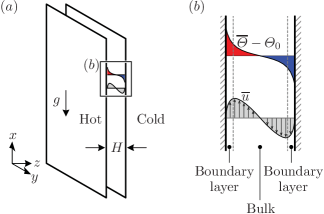
Figure 1: ($a$) Setup of vertical natural convection for the present study. ($b$) Illustration of the mean temperature profile (top) and mean streamwise velocity profile (bottom). Both mean profiles are statistically antisymmetric about the channel centreline. Also illustrated are the boundary layers and bulk region. Note that in general, thermal and kinetic boundary layers have different thicknesses.

With increasing Ra, the boundary layers in thermal convection become increasingly thinner and the flow is understood to undergo a transition from a ‘classical’ regime, where the boundary layers follow a laminar-like Prandtl–Blasius–Pohlhausen (PBP) scaling, to an ‘ultimate’ regime, where the boundary layers are turbulent in the sense of Prandtl and von Kármán (Grossmann & Lohse, 2011, 2012). We are particularly interested to investigate the changes to the boundary-layer structure towards the ultimate regime and the accompanying Ra-dependence of the Nusselt number and the Reynolds number $\Rey$. Our investigation is motivated by the fact that experimental studies in RBC have found a transition from the classical to the ultimate regime at a transitional Rayleigh number-value of approximately $5\times 10^{14}$ (He et al., 2012). Accompanying the transition to the ultimate regime, the overall mean temperature profile exhibits an increasingly pronounced logarithmic dependence (Ahlers et al., 2012, 2014). In a two-dimensional numerical study at lower Ra, the local mean temperature profile was also found to exhibit similar logarithmic variations where thermal plumes are emitted (van der Poel et al., 2015). The presence of a local logarithmic-type mean temperature profile in RBC suggests that we can employ a criterion to distinguish flow regions in VC to compute local statistics, similar to the approach adopted by van der Poel et al. (2015). In addition, the big and unique advantage of VC is that a well-defined mean flow exists which allows for a longer time sampling of our data. In Ng et al. (2015), we have also shown that aspects of the Grossmann–Lohse theory (Grossmann & Lohse, 2000, 2001, 2002, 2004) (hereafter GL theory), which provided physical arguments for the scaling relations in horizontal thermal convection, i.e. RBC, can also be extended to VC. Therefore, the present study makes contact with current efforts to understand the changes to the boundary layer structure in the transition from the classical to the ultimate regime of thermal convection.

The paper is organized as follows: In § 2, we first give the underlying dynamical equations which are numerically solved. From a visual assessment of the near-wall velocity and temperature fields (§ 3), we identify two regions that are increasingly distinguishable at higher Ra, namely a streaky higher-shear flow region and a non-streaky lower-shear flow region. Motivated by the visual changes in the near-wall flow features, we define a flux-based Richardson number, $|\mbox{{Ri}}_{f}|$ (§ 4), which is inspired by the classical definition (see for example in Chapter 5 of Turner, 1979). A criterion is selected based on $|\mbox{{Ri}}_{f}|$ in order to separate the dynamics of the streaky and non-streaky regions. Conveniently, the streaky higher-shear flow regions are well-correlated with low-$|\mbox{{Ri}}_{f}|$ regions, and vice versa. When we quantify the wall-area fraction occupied by the streaky higher-shear regions (§ 5), we find that the wall-area fraction increases with increasing Ra. We then employ a conditional averaging procedure to compute the local mean statistics of the two regions (§ 6) as well as the local scaling of Nu and $\Rey$ (§ 7). Finally, we compare the near-wall structures in VC with the near-wall streaks in pressure-driven channel flow, the latter of which are unique and robust features of the buffer region in wall-bounded turbulence. The comparison is aided by the analysis of the one-dimensional premultiplied spectra of streamwise velocity (§ 8). The paper ends with a summary and conclusions (§ 9).

2 Dynamical equations and boundary conditions

In this study, we analyse the dataset for VC for Rayleigh numbers ranging from $10^{5}$ to $10^{9}$ at constant Prandtl number value of 0.709. The numerical setup for VC is the same as that employed by Ng et al. (2015), see figure 1, i.e. we consider a buoyancy driven flow between two vertical walls with the left wall heated and the right wall cooled. The temperatures at the wall are kept uniform and are denoted $T_{h}$ and $T_{c}$, respectively. Thus, the temperature difference of the walls $\Delta=T_{h}-T_{c}$ establishes a heat flux which acts horizontally across a wall-separation distance $H$. The governing continuity, momentum and energy equations for the velocity field $\bm{u}(\bm{x},t)$ and the temperature field $\varTheta(\bm{x},t)$ are respectively given by, u &= 0,
∂u∂t + u u = -1ρ0 ∇p + ^e_x g β(Θ-Θ_0) + ν∇^2 u,
∂Θ∂t + u Θ= κ∇^2 Θ, where $\hat{\mathbf{e}}_{x}$ is the unit vector in the $x$-direction. The pressure field is denoted by $p(\bm{x},t)$. We define $\varTheta_{0}=(T_{h}+T_{c})/2$ as the reference temperature and $g$ as the gravitational acceleration. We also specify $\beta$ as the coefficient of thermal expansion, $\nu$ as the kinematic viscosity and $\kappa$ as the thermal diffusivity, all assumed to be independent of temperature. The Rayleigh and Prandtl numbers are then respectively defined as Ra≡gβΔH3νκ, ≡νκ. The coordinate system $x$, $y$ and $z$ refers to the streamwise (opposing gravity), spanwise and wall-normal directions. The no-slip and no-penetration boundary conditions are imposed on the velocity at the walls. Periodic boundary conditions are imposed on $\bm{u}$, $p$ and $\varTheta$ in the $x$- and $y$-directions. In addition, we denote time- and $xy$-plane-averaged quantities with an overbar, and the corresponding fluctuating part with a prime, the mean streamwise velocity component is defined by $\overline{u}=u-u^{\prime}$ and the mean temperature is defined by $\overline{\varTheta}=\varTheta-\varTheta^{\prime}$.

Equations (2$a$–$c$) are numerically solved in the domain-size $L_{x}\times L_{y}\times L_{z}=8H\times 4H\times H$. The present simulations employ smaller periodic-domain sizes (two-thirds in each periodic direction) than other DNS studies ( Versteegh & Nieuwstadt, 1999; Pallares et al., 2010) but are chosen in order to resolve the near-wall region at high Ra. Comparison with previous DNS studies showed good agreement for the mean and second-order statistics and other simulation parameters have been previously reported in Ng et al. (2015). All of the analyses in this study are based on statistics that are averaged from both halves of the channel, taking the statistical antisymmetry (about the centreline) of the mean profiles into account.

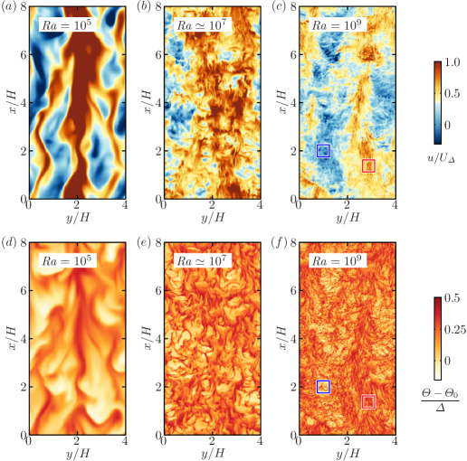
Figure 2: ($a$,$b$,$c$) Wall-parallel planes of streamwise velocity, and ($d$,$e$,$f$) temperature for $\mbox{{Ra}}\simeq 10^{5}$, $10^{7}$ and $10^{9}$. The planes are extracted close to the hotter wall at $z^{+}\approx 15$. Gravity is acting downwards. The non-streaky lower-shear regions are indicated by the blue boxes whereas the streaky higher-shear regions are indicated by the red boxes (see magnified views in figure 3). Here, $U_{\Delta}\equiv\sqrt{g\beta\Delta H}$ the free-fall velocity.

3 Flow visualisations

Figure 2 shows the wall-parallel planes of velocity and temperature for $\mbox{{Ra}}\simeq 10^{5}$, $10^{7}$ and $10^{9}$. The planes were extracted from the three-dimensional volumes for velocity and temperature near the hotter wall at the wall-normal location equivalent to $z^{+}\equiv z/\delta_{\nu}\approx 15$, where $\delta_{\nu}\equiv\nu/u_{\tau}$ is the viscous length scale and $u_{\tau}\equiv\sqrt{\nu\,\mathrm{d}\overline{u}/\mathrm{d}z|_{w}}$ is the friction velocity scale. Note that we use the ⁺ symbol to denote normalisation in viscous wall units. In figures 2($a$–$c$), the velocity fields are coloured from blue to red to denote low- and high-speed regions (or equivalently, lower- and higher-shear regions), respectively, whereas in figures 2($d$–$f$) the temperature fields are coloured from white to red to denote the temperature variations from cooler regions with a temperature around $\varTheta_{0}$ to hotter regions with a temperature around $T_{h}$.

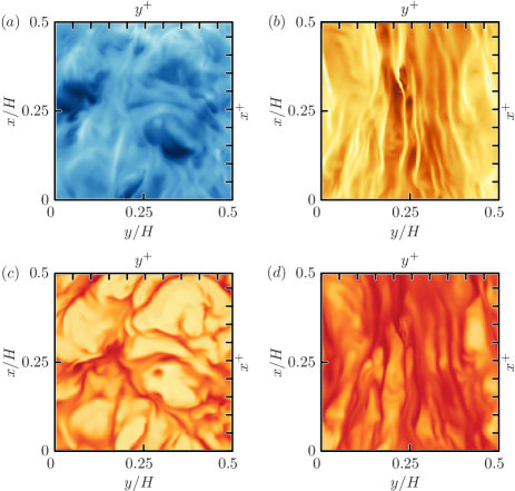
Figure 3: Magnified wall-parallel planes of streamwise velocity ($a$,$b$) and temperature ($c$,$d$), respectively reproduced from the blue and red boxes from figure 2($c$,$f$) for $\mbox{{Ra}}=10^{9}$. In ($a$,$c$) we observe non-streaky lower-shear regions (from the blue boxes), whereas in ($b$,$d$) we observe streaky higher-shear regions (from the red boxes), both with characteristic spanwise spacings of 100 to 200 viscous units. For reference, the axes at the top and right edges denote spacings of 100 viscous units. The colormaps are the same as in figure 2.

Not surprisingly, from figure 2, the structures in the velocity and temperature fields are observed to become increasingly finer at higher Ra. The finer structures are particularly prominent at $\mbox{{Ra}}=10^{9}$ (figures 2$c$ and $f$). Coincident with the higher-shear regions, the finer structures appear streaky and are markedly different to the structures in the lower-shear regions as well as the structures in the visualisations at lower-Ra. To focus on the differences, magnified views of the higher- and lower-shear regions are plotted for $\mbox{{Ra}}=10^{9}$ in figure 3.

On closer inspection of the magnified views (figure 3), the streaky structures appear reminiscent of the near-wall streaks, which are well-documented flow features in canonical turbulent boundary layers (Hutchins & Marusic, 2007a; Marusic et al., 2010; Smits et al., 2011). In the magnified view, the spanwise spacing of the streaky structures is approximately 100–200 viscous units, consistent with the spacing of the near-wall streaks found by Kline et al. (1967). The similarity between the streaky structures in VC at higher Ra and in canonical turbulent boundary layers suggests that locally, the boundary layers in VC are much more strongly animated by a large-scale ‘wind’, perhaps an indication of an incipient turbulent boundary layer. Additionally, this incipient behaviour appears to manifest as increasingly larger streaky regions, as observed in the plane visualisations in figure 2. Therefore, a reasonable starting point would be to seek a quantity that is able to distinguish between the two regions and that would also enable us to study the corresponding local scaling.

4 Identifying different flow regions

In order to quantitatively distinguish the two regions shown in the magnified views in figure 2, we define a flux-based Richardson number at the wall-normal location $z^{+}=15$ (i.e.  just outside the viscous sublayer),

$$\mbox{{Ri}}_{f}\equiv\dfrac{z(z^{+}=15)}{L}=\dfrac{15}{L^{+}},$$ (1)

where $L\equiv-u_{\tau}^{3}/(g\beta f_{w})$ is the Obukhov length and $f_{w}\equiv-\kappa(\mathrm{d}\overline{\varTheta}/\mathrm{d}z)|_{w}$ is the wall heat flux and $u_{\tau}$ is the friction velocity scale defined in § 3. The Obukhov length is defined such that when $f_{w}<0$, then $L>0$ (§ 7.2 Monin & Yaglom, 2007). Since $f_{w}>0$ for VC, then $L<0$ and the sign of $\mbox{{Ri}}_{f}$ becomes negative for VC. Therefore, to assist interpretation, we will use $\mbox{{Ri}}_{f}$ mainly modulo-wise, $|\mbox{{Ri}}_{f}|$.

We emphasise that our flux-based Richardson number definition in (1) is a local quantity (in the plane $z^{+}=15$) to measure shear-dominated areas versus buoyancy dominated areas and is merely an analogy that is inspired by the classical definition (see for example Chapter 5 in Turner, 1979). Equation (1) is notionally similar to the Obukhov stability parameter, which is a dimensionless height typically adopted in the study of atmospheric surface layer turbulence (Businger et al., 1971). Our definition is therefore far from perfect since the vertical heat flux in VC is a response to the horizontal heat flux imposed on the system, whereas in the classical definition, both the imposed and responding heat fluxes act in the same (vertical) direction. Nevertheless, we take advantage of (1) in our study simply as a convenient parameter which is able to quantify the dominance of buoyancy relative to shear. It is also for this reason that we prefer to use (1) to distinguish high-speed regions instead of other quantities, such as the shear Reynolds number (see for example Scheel & Schumacher, 2016). By defining (1), we also make contact with recent efforts to distinguish ‘wind-sheared’ regions in flows that are analogous to VC, for example, in Taylor–Couette flows (Ostilla-Mónico et al., 2014) and RBC (van der Poel et al., 2015).

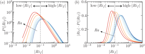
Figure 4: ($a$) Probability distribution functions of $|\mbox{{Ri}}_{f}|$, and ($b$) the premultiplied form defined in equation (2). The curves are coloured blue to red to represent increasing Ra. The low- and high-$|\mbox{{Ri}}_{f}|$ ranges are demarcated by $|\mbox{{Ri}}_{f}|=0.1$ (dashed line). The premultiplied PDFs in ($b$) are increasingly weighted towards lower-$|\mbox{{Ri}}_{f}|$ with increasing Ra.

We now turn to the probability distributions functions (PDFs) of $|\mbox{{Ri}}_{f}|$ (figure 4$a$) to determine a suitable threshold value that can distinguish the high-speed and low-heat flux regions. To visually aid the interpretation on a doubly logarithmic plot, we premultiply the PDFs with $|\mbox{{Ri}}_{f}|$ so that the area of a semi-logarithmic plot represents the probability, i.e.

$$\int_{0}^{+\infty}P(|\mbox{{Ri}}_{f}|)\,\mathrm{d}|\mbox{{Ri}}_{f}|=1=\int_{0}^{+\infty}|\mbox{{Ri}}_{f}|\cdot P(|\mbox{{Ri}}_{f}|)\,\mathrm{d}(\log|\mbox{{Ri}}_{f}|).$$ (2)

The integrand on the left-hand-side of (2) is plotted in figure 4($a$) and the integrand on the right-hand-side of (2) is plotted in figure 4($b$). Therefore, in the representation of figure 4($b$), the area beneath the PDF curve represents equal probability of $|\mbox{{Ri}}_{f}|$, which is not the case in figure 4($a$). The curves are coloured from blue to red to represent increasing Ra. We further define a low-$|\mbox{{Ri}}_{f}|$ as $0<|\mbox{{Ri}}_{f}|\leqslant 0.1$ and high-$|\mbox{{Ri}}_{f}|$ as $|\mbox{{Ri}}_{f}|>0.1$. From figure 4($b$), we observe that with increasing Ra, there is an increase in the areas under the premultipied curves which correspond to the low-$|\mbox{{Ri}}_{f}|$. This increase in area suggests that the distributions of $|\mbox{{Ri}}_{f}|$ are increasingly weighted towards the lower-$|\mbox{{Ri}}_{f}|$ values with increasing Ra. As a further example, the value of the mode of the Richardson number $|\mbox{{Ri}}_{f,m}|$ in figure 4($a$) decreases as $|\mbox{{Ri}}_{f,m}|\approx 0.99\mbox{{Ra}}^{-0.16}$ from a least-squares fit to a single power law.

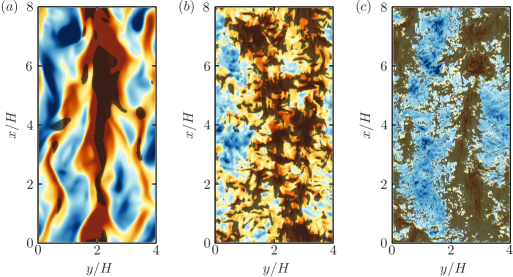
Figure 5: Same wall-parallel planes of streamwise velocity as in figures 2($a$–$c$), but now overlayed with grey contours of $0<|\mbox{{Ri}}_{f}|\leqslant 0.1$. The Ra-values are ($a$) $10^{5}$, ($b$) $2\times 10^{7}$ and ($c$) $10^{9}$. With increasing Ra, the grey contours are increasingly correlated with the streaky higher-shear regions and occupy increasingly larger wall-area fractions. Gravity is acting downwards.

To explain the trend observed in the premultiplied PDFs, we refer to a visual example of low-$|\mbox{{Ri}}_{f}|$ regions which are shown as grey-filled patches in figure 5. The grey-filled patches are overlayed on the plane-parallel visualisations of streamwise velocity for three Ra-values, which are reproduced from figure 2. At the highest Ra (figure 5$c$), we observe that the low-$|\mbox{{Ri}}_{f}|$ regions are well-correlated with the streaky regions in figure 2($c$). In figure 5, the degree of correlation also increases with increasing Ra and is matched by an increasingly larger wall-area coverage of low-$|\mbox{{Ri}}_{f}|$ regions. The improved correlations and increasing wall-area coverage of the low-$|\mbox{{Ri}}_{f}|$ regions are consistent with the increasingly weighted trends of the premultiplied PDFs of lower-$|\mbox{{Ri}}_{f}|$ values with increasing Ra, seen in figure 4($b$). These well-matched behaviours of low-$|\mbox{{Ri}}_{f}|$ distributions and the streaky regions imply that it may be possible to quantify shear-dominated regions from a carefully selected low-$|\mbox{{Ri}}_{f}|$ value.

As a starting point, we choose the range $0<|\mbox{{Ri}}_{f}|\leqslant 0.1$ as the criteria for identifying shear-dominated regions in our study. If a lower or higher upper limit is selected, the corresponding wall-areas of the local flow that meet the criteria are smaller and larger, respectively. (A brief discussion about the sensitivity of wall-areas to the upper limit is given in Appendix A.) Not surprisingly, the choice of the upper limit has an influence on the local effective scaling. However, we will show in § 7 that for a sufficiently small $|\mbox{{Ri}}_{f}|$ threshold, the effective local scaling exponent of the Nusselt number is unequivocally higher than the global effective scaling exponent and therefore, does not alter the conclusions of this study.

5 Low-$|\mbox{{Ri}}_{f}|$ area fraction

Using the flux-Richardson number criteria defined in § 4, we quantify the wall-areas occupied by the low-$|\mbox{{Ri}}_{f}|$ regions for our Ra-range. These wall-areas correspond to shear-dominated regions and we quantify the area fraction $\rho(\mbox{{Ra}})$ according to

$$\rho(\mbox{{Ra}})\equiv\dfrac{\int_{0}^{L_{y}}\int_{0}^{L_{x}}I_{0<|\mbox{{Ri}}_{f}|\leqslant 0.1}\,\mathrm{d}x\,\mathrm{d}y}{\int_{0}^{L_{y}}\int_{0}^{L_{x}}\,\mathrm{d}x\,\mathrm{d}y},$$ (3)

where $I$ is an indicator function, being 1 for wall-areas where $0<|\mbox{{Ri}}_{f}|\leqslant 0.1$ (low-$|\mbox{{Ri}}_{f}|$) and being 0 where $|\mbox{{Ri}}_{f}|>0.1$ (high-$|\mbox{{Ri}}_{f}|$). Therefore, the numerator represents the streamwise-spanwise wall-area influenced by low-$|\mbox{{Ri}}_{f}|$ flow and the denominator represents the total wall-area of our setup, which is $L_{x}\times L_{y}=32H^{2}$. Equation (3) is similar to the definition used to quantify the spatial intermittency of strong shear regions in RBC ( Scheel & Schumacher, 2016). The results for the area fractions $\rho(\mbox{{Ra}})$ are shown in figure 6 as filled circles.

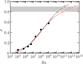
Figure 6: Plot of $\rho$ the area fraction of higher-shear low-$|\mbox{{Ri}}_{f}|$ regions (solid circles) versus Ra. $\rho$ is defined in equation (3). The solid black curve is the empirical fit to $\rho_{fit,1}$, see equation (4), and the solid red curve is the empirical fit to $\rho_{fit,2}$, see equation (5). From an extrapolation to $\rho=0.8$ and $0.9$, we obtain $\mbox{{Ra}}\approx 1.5\times 10^{10}$ and $\approx 1.2\times 10^{11}$, respectively, for $\rho_{fit,1}$ (black open circles) and $\mbox{{Ra}}\approx 6.5\times 10^{10}$ and $\approx 2.8\times 10^{12}$, respectively, for $\rho_{fit,2}$ (red open circles).

In figure 6, the area fractions for the low-$|\mbox{{Ri}}_{f}|$ regions range from $\rho\approx 0.062$ for $\mbox{{Ra}}=10^{5}$ to $\rho\approx 0.58$ for $\mbox{{Ra}}=10^{9}$. Visually, the trend of the area fractions appears sigmoidal and therefore, using a fit to an error function, the trend for $\rho(\mbox{{Ra}})$ can be approximated by

$$\rho_{fit,1}=0.49\operatorname{erf}\left[0.35\log_{10}(\mbox{{Ra}})-2.95\right]+0.5.$$ (4)

Alternatively, the trend for $\rho(\mbox{{Ra}})$ can also be approximated by a fit to the Gompertz function

$$\rho_{fit,2}=0.99\exp\{-2.21\exp\left[-0.48\log_{10}(\mbox{{Ra}})+2.91\right]\},$$ (5)

which is an asymmetric sigmoid function. In contrast to (4), equation (5) captures a lower inflection point in the trend of $\rho$, which occurs at $\mbox{{Ra}}=2\times 10^{7}$ in figure 6. However, equation (5) does not capture the trend of $\rho$ for $\mbox{{Ra}}\lesssim 5.4\times 10^{5}$ compared to (4). We note that both curve fits are only statistical approximations and there are inherent risks involved when extrapolating results to higher Ra. Therefore, in the interest of obtaining a conservative estimate, we include both $\rho_{fit,1}$ and $\rho_{fit,2}$ in our subsequent discussions.

From extrapolations of (4) and (5), approximately $80\%$ to $90\%$ of the near-wall region are presumed to be dominated by streaks between $\mbox{{Ra}}\approx 1.5\times 10^{10}$ to $1.2\times 10^{11}$, based on (4), or $\mbox{{Ra}}\approx 6.5\times 10^{10}$ to $2.8\times 10^{12}$, based on (5). Overall, the trend of $\rho(\mbox{{Ra}})$ is increasing and indicates that higher-shear regions occupy increasingly larger wall areas at higher Ra.

Our results are consistent with the notion that for the present Ra range, the boundary layers in VC can be considered to be in a transitional state. As the flow approaches the fully turbulent, or ultimate regime, the relative size of the shear-dominated regions grow until the regions fully occupy the wall (van der Poel et al., 2015).

6 Mean profiles and conditional mean profiles

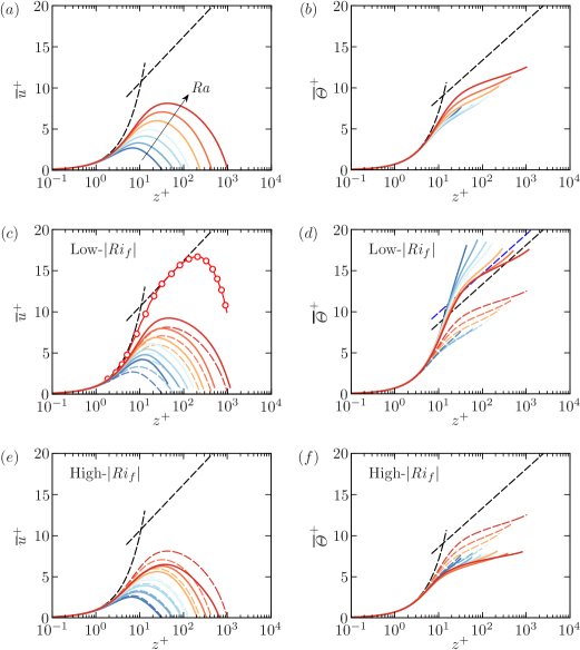
Figure 7: ($a$) Overall mean velocity profiles, and ($b$) overall mean temperature profiles, coloured from blue to red to represent increasing Ra. The overall mean profiles are repeated in ($c$) to ($f$) as dashed curves. ($c$,$d$) Conditional mean profiles in low-$|\mbox{{Ri}}_{f}|$ ($0<|\mbox{{Ri}}_{f}|\leqslant 0.1$) regions. ($e$,$f$) Conditional mean profiles in high-$|\mbox{{Ri}}_{f}|$ ($|\mbox{{Ri}}_{f}|>0.1$) regions. The black straight dashed lines correspond to the log-laws of the walls for velocity and temperature, equation (6), with $\kappa_{\nu}=0.41$, $A=5.0$, $\Pran_{t}=0.85$ and $B=3.8$. In ($c$), the red curve with open symbols correspond to the mean streamwise velocity from the wall-jet flow (reproduced from figure 13, Eriksson et al., 1998). In ($d$), the blue straight dashed line corresponds to equation (6$b$) with $B=5.1$.

The overall mean profiles for streamwise velocity and temperature are shown in figures 7($a$) and ($b$), where the profiles are coloured from blue to red to indicate increasing Ra. From both figures, we conclude that there are no log-profiles in the mean statistics when scaled in wall units. We highlight the absence of the log-profiles in the overall mean profiles by including in figure 7($a$) and ($b$) the log-laws of the wall, which are expected when the flow is fully turbulent in the sense of Prandtl and von Kármán. The log-laws of the wall for streamwise velocity and temperature may be written as, ¯u^+ = 1κvlog(z^+) + A   and  ¯Θ^+ = tκvlog(z^+) + B, (cf.  Yaglom, 1979), where $\overline{u}^{+}\equiv\overline{u}/u_{\tau}$ and $\overline{\varTheta}^{+}\equiv(\overline{\varTheta}-\varTheta_{h})/\theta_{\tau}$. Equations (6) are plotted as black dashed lines in figure 7. For the purposes of our study, we choose to adopt the same constants as Yaglom (1979), i.e. the von Kármán constant $\kappa_{v}=0.41$, the turbulent Prandtl number $\Pran_{t}=0.85$, $A=5.0$ and $B=3.8$. We also employ the temperature scale $\theta_{\tau}\equiv-f_{w}/u_{\tau}$. Near the wall, the mean profiles are linear and obey $\overline{u}^{+}=z^{+}$ and $\overline{\varTheta}^{+}=\Pran\,z^{+}$.

To assess the mean profiles in the streaky and high-shear regions only, we compute the conditional mean profiles within the low-$|\mbox{{Ri}}_{f}|$ regions according to the conditional averaging procedure

$$\overline{(\cdot)}_{l}(z)=\dfrac{\int_{0}^{L_{y}}\int_{0}^{L_{x}}I_{0<|\mbox{{Ri}}_{f}|\leqslant 0.1}(\cdot)(\bm{x},t)\,\mathrm{d}x\,\mathrm{d}y}{\int_{0}^{L_{y}}\int_{0}^{L_{x}}I_{0<|\mbox{{Ri}}_{f}|\leqslant 0.1}\,\mathrm{d}x\,\mathrm{d}y},$$ (6)

where the subscript $l$ distinguishes the quantities $(\cdot)$ in the low-$|\mbox{{Ri}}_{f}|$ regions and $I$ is the indicator function previously defined in (3). The conditional mean profiles for the high-$|\mbox{{Ri}}_{f}|$ regions, denoted by a subscript $h$, follow the similar definition as (6) but with the indicator function criteria $I_{|\mbox{{Ri}}_{f}|>0.1}$. Thus, the conditional mean and variance profiles are related to the area fraction $\rho$ by ¯u(z) &= ρ¯u_l + (1-ρ)¯u_h,
¯u^′u^′(z) = ρ¯(u^′u^′)_l + (1-ρ)¯(u^′u^′)_h - 2ρ(1-ρ)¯u_l ¯u_h, where, ¯(u^′u^′)_l ≡¯u_l^2 - ρ(¯u_l)^2  and ¯(u^′u^′)_h ≡¯u_h^2 - (1-ρ)(¯u_h)^2.

The low-$|\mbox{{Ri}}_{f}|$ mean velocity and temperature profiles are shown by the solid curves in figures 7($c$) and 7($d$), respectively, whereas the overall mean profiles are redrawn as dashed lines. The conditional mean profiles of the low-$|\mbox{{Ri}}_{f}|$ regions are clearly different from the overall mean profiles of VC. The conditional mean velocity profiles (figure 7$c$) exhibit steeper slopes close to the wall and also larger maxima. These two observations imply that the local boundary layer in the low-$|\mbox{{Ri}}_{f}|$ region is more vigorously animated by a turbulent wind as compared to the overall boundary layer. However, the conditional mean profiles still do not exhibit the log-profile according to (6$a$). The absence of the log-profile suggests that for the present Ra range, we would not expect the $\Rey\sim\mbox{{Ra}}^{1/2}$-ultimate regime scaling as predicted according to Grossmann & Lohse (2011).

In contrast, the conditional mean temperature profiles (figure 7$d$) exhibit some degree of collapse at higher Ra between $30\lesssim z^{+}\lesssim 80$ which agrees with the log-linear slope of (6$b$) with $B=5.1$ (see blue straight dashed line). This collapse is interesting because it suggests that locally, the thermal boundary layers are log-dependent on the wall-normal distance as assumed by Grossmann & Lohse (2011, 2012) for turbulent thermal convection.

With reference to figure 7, we emphasize that we perform a direct comparison with the log-laws of the wall. For the mean velocity profiles, we envision that the profiles will eventually exhibit the log-law once a wider separation of scales is achieved at very high Ra. As an example of sufficient scale separation, we refer to the mean streamwise velocity profile of the wall-jet flow (Wygnanski et al., 1992; Eriksson et al., 1998). The mean velocity profiles of the wall-jet flow are statistically similar to the mean streamwise velocity profile of VC, but have been shown to exhibit the log-law of the wall. As a comparison, we include a candidate mean streamwise velocity profile from the wall-jet flow of Eriksson et al. (1998) in figure 7($c$), see red curve with open symbols. The wall-jet profile exhibits a higher maxima compared to the VC profile at $\mbox{{Ra}}=10^{9}$ and agrees well with the log-law of the wall. Therefore, from the perspective of classical dimensional arguments of the ‘inner’ and ‘outer layer’ (Pope, 2000, Chapter 7), we infer that the outer layer of VC corresponds to the location near the maxima of the streamwise velocity, as opposed to the region close to the channel-centre. The log-profiles in VC are also expected since similar trends have also been measured for RBC and Taylor–Couette flows, but in different regions of the flow. In the ultimate regime of RBC, the temperature log-profile was found in the bulk flow region (Ahlers et al., 2012; Wei & Ahlers, 2014), whereas in the classical regime of RBC, the log-profile was found in high-$|\mbox{{Ri}}_{f}|$ regions where thermal plumes are emitted (van der Poel et al., 2015). In Taylor–Couette flows, a log-profile was found in the azimuthal velocity profile in plume emission regions, as well as in the (appropriately shifted) overall angular velocity profile (Ostilla-Mónico et al., 2014).

For comparison, we also include the conditional mean profiles of the high-$|\mbox{{Ri}}_{f}|$ regions in figures 7($e$) and 7($f$). The mean profiles are lower in magnitude than the overall profiles, which can be attributed to a weaker influence of the turbulent wind in the high-$|\mbox{{Ri}}_{f}|$ regions. In addition, the mean temperature profiles exhibit some degree of collapse but does not fit the log-linear trend of (6$b$).

7 Scaling of local Nu and $\Rey$

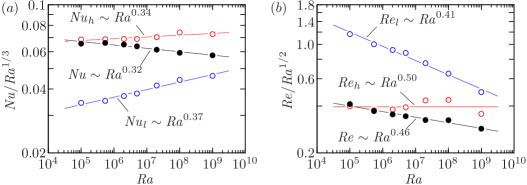
Figure 8: Compensated plots for ($a$) Nu and ($b$) $\Rey$. Black symbols denote the overall Nu and $\Rey$ results, blue symbols denote the higher-shear, low-$|\mbox{{Ri}}_{f}|$ results and red symbols denote the lower-shear, high-$|\mbox{{Ri}}_{f}|$ results. All curve-fits are from a least-squares fit to an effective power law.

We can further test the characteristics of the low-/high-$|\mbox{{Ri}}_{f}|$ regions in VC by computing the local Nusselt and Reynolds number trends in the corresponding regions. Within the low-$|\mbox{{Ri}}_{f}|$ regions, the local Nusselt number and Reynolds number are defined respectively as Nu_l ≡fw,lHΔκ and _l ≡Urms,lHν, where $f_{w,l}\equiv-\kappa(\mathrm{d}\overline{\varTheta}_{l}/\mathrm{d}z)|_{w}$. To define the local Reynolds number, we define $U_{rms,l}$ as the local turbulent wind and adopt (6) to compute the local velocity fluctuations. Therefore, we define $U_{rms,l}\equiv\left[\overline{(u^{\prime}u^{\prime})}_{l}\right]^{1/2}$ evaluated at the wall-normal location $z=\delta_{max,l}$, where $\delta_{max,l}$ is the wall-normal distance to the maximum of $\overline{u}_{l}$. The local Nusselt and Reynolds numbers in the high-$|\mbox{{Ri}}_{f}|$ regions follow the definition in (8) with the corresponding high-$|\mbox{{Ri}}_{f}|$ quantities. The overall Nusselt and Reynolds numbers are defined using the overall $f_{w}$ and $U_{rms}$. The results of the scaling of the Nusselt and Reynolds numbers are shown in figure 8.

In figure 8, we emphasise the scaling of the Nusselt and Reynolds numbers by plotting the trends in compensated forms, i.e.  $\mbox{{Nu}}/\mbox{{Ra}}^{1/3}$ versus Ra and $\Rey/\mbox{{Ra}}^{1/2}$ versus Ra. The overall Nu and $\Rey$ are denoted by solid black symbols, $\mbox{{Nu}}_{l}$ and $\Rey_{l}$ by open blue circles, and $\mbox{{Nu}}_{h}$ and $\Rey_{h}$ by open red circles. Starting with the scaling of the local Nusselt number (figure 8$a$), we find that $\mbox{{Nu}}_{l}\sim\mbox{{Ra}}^{0.37}$ from a least-squares fit to an effective power law, which is steeper than the relation $\mbox{{Nu}}\sim\mbox{{Ra}}^{0.32}$ for the overall Nusselt number (Ng et al., 2015). Interestingly, the effective scaling exponent computed for the low-$|\mbox{{Ri}}_{f}|$ regions, which is $0.37$, is close to the exponent reported by He et al. (2012) in their experiments for RBC at large Ra, which is $0.38$. This result appears consistent with the predictions of the Nusselt number scaling relation of a $1/2$-power law scaling with logarithmic corrections in the ultimate regime (Grossmann & Lohse, 2011). For VC, the logarithmic corrections for the effective scaling of $\mbox{{Nu}}_{l}$ are associated with the log-linear slope of the conditional mean temperature profile in the high-shear, low-$|\mbox{{Ri}}_{f}|$ regions (see figure 7$d$). On the other hand, the scaling of $\mbox{{Nu}}_{h}$ follows $\mbox{{Nu}}_{h}\sim\mbox{{Ra}}^{0.34}$ which is steeper than the scaling for overall Nu but is still less steep compared to the scaling of $\mbox{{Nu}}_{l}$.

We note that the local scaling of the Nusselt number is sensitive to the upper limit of the $|\mbox{{Ri}}_{f}|$ criterion established in § 4. For a higher limit, the conditional mean statistics of the higher-shear regions are contaminated by the laminar-like lower-shear regions (see Appendix A) and as a result, the effective Ra-scaling exponent of the local Nusselt number is closer to the global $0.31$ exponent. For example, the effective Ra-scaling exponent for $\mbox{{Nu}}_{l}$ is approximately $0.33$ using $0<|\mbox{{Ri}}_{f}|\leqslant 0.5$ and is approximately $0.39$ using $0<|\mbox{{Ri}}_{f}|\leqslant 0.05$. In the former, the scaling exponent of $0.33$ is closer to $0.31$, whereas in the latter, the scaling exponent of $0.39$ is clearly steeper than $0.31$ and is consistent with the scaling exponent reported by He et al. (2012).

For the scaling of the Reynolds numbers (figure 8$b$), we find that $\Rey_{l}\sim\mbox{{Ra}}^{0.41}$, $\Rey_{h}\sim\mbox{{Ra}}^{0.50}$ and $\Rey\sim\mbox{{Ra}}^{0.46}$. Based on the much lower effective scaling exponent for $\Rey_{l}$, it is clear that the Reynolds number in the high-shear regions do not exhibit the $1/2$-power-law ultimate regime scaling as predicted in GL theory (Grossmann & Lohse, 2011). However, this result is not surprising since the conditional mean velocity profiles for the low-$|\mbox{{Ri}}_{f}|$ regions (see figure 7$c$) do not exhibit the log-linear profile of (6$a$), which is assumed for fully turbulent thermal convection (Grossmann & Lohse, 2011) and is a key assumption of the GL theory for the $\Rey$-scaling in the ultimate regime.

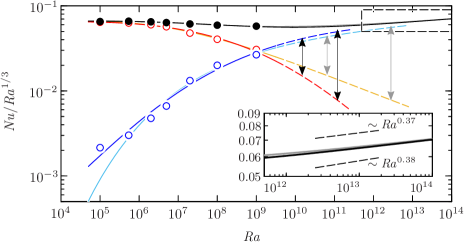
Figure 9: Relative contributions of the local Nusselt numbers with increasing Ra. The solid black symbols denote the overall Nu, the blue symbols denote $\rho\mbox{{Nu}}_{l}$ and the red symbols denote $(1-\rho)\mbox{{Nu}}_{h}$. The blue and red curves represents $\rho_{fit,1}\mbox{{Ra}}^{0.37}$ and $(1-\rho_{fit,2})\mbox{{Ra}}^{0.34}$, respectively, and the sum equals to the black curve. The cyan and orange curves represent $\rho_{fit,2}\mbox{{Ra}}^{0.37}$ and $(1-\rho_{fit,2})\mbox{{Ra}}^{0.34}$, respectively, and the sum equals to the grey curve. The inset plot compares the extrapolated curves in the dashed box with the Ra-scaling exponent of 0.37 and 0.38. The trends indicate that the contributions from $\mbox{{Nu}}_{l}$ dominate the contributions from $\mbox{{Nu}}_{h}$ with increasing Ra.

Based on our results in figure 8($a$) for the effective scaling exponents of $\mbox{{Nu}}_{l}$ and $\mbox{{Nu}}_{h}$, we estimate the relative contributions of $\mbox{{Nu}}_{l}$ and $\mbox{{Nu}}_{h}$ by making use of the relation

$$\mbox{{Nu}}=\rho\mbox{{Nu}}_{l}+(1-\rho)\mbox{{Nu}}_{h},$$ (7)

which can be derived using the conditional averaging procedure described by (6). We then model the two terms on the right-hand-side of (7) using both curve-fits (4) and (5), and the effective power-law curve-fits for $\mbox{{Nu}}_{l}$ and $\mbox{{Nu}}_{h}$ from figure 8($a$), thus, ρNu_l ∼ρ_fitRa^0.37 and (1-ρ)Nu_h ∼(1-ρ_fit)Ra^0.34. The two modelled terms on the right-hand-side of (7) are plotted in figure 9, where the blue-red lines correspond to $\rho_{fit,1}$ and the cyan-orange lines correspond to $\rho_{fit,2}$. The blue and red symbols in figure 9 correspond to the results from our DNS, i.e.  the left-hand-side of (7), respectively. The solid black symbols are the overall Nu-values, which are exactly equal to the sum of the values denoted by the blue and red symbols.

From figure 9, we find that the contribution of $\rho\mbox{{Nu}}_{l}$ increases with increasing Ra, as expected. When we extrapolate the two modelled terms in (7), shown by the dashed lines in figure 9, the contribution from $\mbox{{Nu}}_{l}$ dominates the contribution from $\mbox{{Nu}}_{h}$ at higher Ra. For instance, the ratio of $\rho\mbox{{Nu}}_{l}$ to $(1-\rho)\mbox{{Nu}}_{h}$ for $\rho_{fit,1}$ ranges from approximately 3 to 7 between $\mbox{{Ra}}\approx 1.5\times 10^{10}$ to $1.2\times 10^{11}$ (black arrows in figure 9) and, coincidently for $\rho_{fit,2}$, also ranges from approximately 3 to 7 between $\mbox{{Ra}}\approx 6.5\times 10^{10}$ to $2.8\times 10^{12}$ (grey arrows in figure 9). The two pairs of Ra-values correspond to the estimated $80\%$ to $90\%$ of the near-wall area that are presumably covered by the streaky, higher-shear regions (cf.  § 5). For the sake of obtaining estimates, we further extrapolate the sum of the modelled terms from (7) and the trends are shown as solid black and solid grey curves in figure 9. At $\mbox{{Ra}}\gtrsim 10^{13}$, the slope of the two extrapolated trends become comparable to the Ra-scaling exponent of between 0.37-0.38 (see inset of figure 9), which is expected since the relative contribution of $(1-\rho)\mbox{{Nu}}_{h}$ diminishes at very high-Ra.

For standard RBC, Shang et al. (2008) performed a similar decomposition of the heat transfer, namely in a plume-dominated part $\mbox{{Nu}}_{pl}\sim\mbox{{Ra}}^{0.24}$ and a bulk-dominated part $\mbox{{Nu}}\sim\mbox{{Ra}}^{0.49}$, with the bulk part gaining dominance beyond $\mbox{{Ra}}_{c}\approx 10^{14}$ (see also Shang et al., 2003; Grossmann & Lohse, 2004). The much lower Ra-values for when the ultimate regime scaling dominates in VC as compared to standard RB (where it is $\mbox{{Ra}}_{c}\approx 10^{14}$) may be associated with the more efficient driving in the VC configuration since gravity is parallel to the walls in VC, whereas gravity is orthogonal to the walls in RBC. For the shear-driven Taylor–Couette flow, the driving is even more efficient and the transition to the ultimate regime occurs at the Taylor number $\mbox{{Ta}}_{c}\simeq 3\times 10^{8}$ for an inner-to-outer radius ratio of 0.71 (Grossmann et al., 2016).

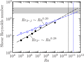
Figure 10: Plots of shear Reynolds number versus Ra. The blue circles denote the low-$|\mbox{{Ri}}_{f}|$ shear Reynolds number ($\Rey_{\delta^{\ast},l}$) whereas the solid black circles denote the overall shear Reynolds number ($\Rey_{\delta^{\ast}}$). The grey region indicates the range of the shear Reynolds number between 200 and 450. At the shear Reynolds number value of 200, the Ra-value is estimated to be $1.5\times 10^{11}$ for the low-$|\mbox{{Ri}}_{f}|$ shear Reynolds number and $3.8\times 10^{10}$ for the overall shear Reynolds number (demarcated by the dotted lines).

In figure 10, we compute the shear Reynolds number based on the displacement thickness $\delta^{\ast}$ according to the definition $\Rey_{\delta^{\ast}}\equiv U\delta^{\ast}/\nu$ for the low-$|\mbox{{Ri}}_{f}|$ and overall regions. For the low-$|\mbox{{Ri}}_{f}|$ regions, we define $U\equiv\text{max}(\overline{u}_{l})$ and $\delta^{\ast}\equiv\int_{0}^{\delta_{max,l}}(1-\overline{u}_{l}/\text{max}(\overline{u}_{l}))\mathrm{d}z$. For the overall shear Reynolds number, we define $U\equiv\text{max}(\overline{u})$ and $\delta^{\ast}\equiv\int_{0}^{\delta_{max}}(1-\overline{u}/\text{max}(\overline{u}))\mathrm{d}z$. At some critical value, the shear Reynolds number can provide an indication of the laminar-to-turbulent transition (for example, $(\Rey_{\delta^{\ast}})_{cr}\approx 420$ Landau & Lifshitz, 1987). However, since the theoretical value for the critical shear Reynolds number is presently unknown for VC, we choose a range of $\Rey_{\delta^{\ast}}$ from 200 to 450 as an approximate indicator for the transition to turbulence in VC. This range is shown as the grey region in figure 10. The results from the low-$|\mbox{{Ri}}_{f}|$ regions are denoted by the open blue circles and the results from the overall regions are denoted by the solid black circles. The associated effective power-law fits are $\Rey_{\delta^{\ast},l}\approx 1.3\mbox{{Ra}}^{0.20}$ (blue line) and $\Rey_{\delta^{\ast}}\approx 0.23\mbox{{Ra}}^{0.28}$ (black line).

From figure 10, we find that $\Rey_{\delta^{\ast},l}$ is larger than $\Rey_{\delta^{\ast}}$ for the present Ra-range of our DNS dataset. By extrapolating the power-law fits (dashed lines in figure 10), we find that at the shear Reynolds number value of 200, the Ra-value is estimated to be $\approx 3.8\times 10^{10}$ for the overall region and $\approx 1.5\times 10^{11}$ for the low-$|\mbox{{Ri}}_{f}|$ region. Both Ra-values appear consistent with the Ra-values estimated when the values of the turbulent fraction $\rho=0.8$ and $0.9$ (see figure 6). Conservatively, our results suggest that we could expect the ultimate regime in VC to occur at $\mbox{{Ra}}\gtrsim 10^{11}$. Physically, the near-wall region is expected to be dominated by streaky, high-shear regions, however, further investigations at much higher Ra are necessary in order to verify this hypothesis.

8 Conditional spectra

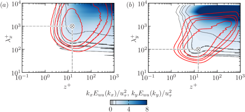
Figure 11: One-dimensional premultiplied overall spectra of $u$ for $\mbox{{Ra}}=10^{9}$ shown as blue contours: ($a$) streamwise direction and ($b$) spanwise direction. The red contours are the spectra from DNS of channel flow at $\Rey_{\tau}\approx 934$ (cf.  del Álamo et al., 2004). For both VC and channel flow spectra, the contour levels are fixed at $0.2$ (outermost), $0.4$, $0.6$ and $1.2$ (indicated by the thinner lines in the colorbar). The $\otimes$ symbols denote the inner sites of channel flow spectra, which are respectively at ($z_{p}^{+}$,$\lambda_{x,p}^{+}$) $\approx$ ($15$,$1000$) and ($z_{p}^{+}$,$\lambda_{y,p}^{+}$) $\approx$ ($15$,$100$).

In this section, we investigate the similarities between the near-wall structures in VC and in a canonical wall-bounded flow setup. In particular, we look for evidence of buffer-region features in the near-wall region of VC, which would suggest that the VC flow is transitioning to the ultimate regime with log-variations in the mean profile. Our basis of comparison is the unique structural features in the buffer region of the flow at $z^{+}\approx 15$, i.e.  before the start of the log-law of the wall. The features in this region are commonly referred to as near-wall streaks (Kline et al., 1967; Hutchins & Marusic, 2007a; Marusic et al., 2010). In canonical wall-bounded flows, the near-wall streaks are robust features of the buffer region: they are found at every location in the wall-parallel plane $z^{+}\approx 15$, contribute to the peak in streamwise velocity fluctuations and exhibit a characteristic spanwise spacing of $\lambda_{y}^{+}\approx 100$. Here, $\lambda_{y}=2\pi k_{y}^{-1}$ the spanwise wavelength. In the following, we conduct a detailed comparison between VC and canonical channel flow with the aid of the one-dimensional spectra.

We define the one-dimensional energy spectra of streamwise velocity $u$ as $E_{uu}(k_{j})$, where $(u^{\prime})^{2}=2\int_{0}^{\infty}E_{uu}(k_{j})\,\mathrm{d}{k_{j}}$, $k_{j}$ is the wavenumber in the $j$-th direction and $j=1,2$. Thus, $k_{1}=k_{x}$ the streamwise wavenumber and $k_{2}=k_{y}$ the spanwise wavenumber. As a reference, we first plot the overall spectra of $u$ for VC at $\mbox{{Ra}}=10^{9}$ in figure 11, shown as filled blue contours. Following Hutchins & Marusic (2007a), we plot the energy spectra at all wall-normal locations in premultiplied form, i.e. $k_{x}E_{uu}(k_{x})$ versus $\lambda_{x}=2\pi k_{x}^{-1}$ the streamwise wavelength (figure 11$a$) and $k_{y}E_{uu}(k_{y})$ versus $\lambda_{y}=2\pi k_{y}^{-1}$ the spanwise wavelength (figure 11$b$). In premultiplied form and on a logarithmic plot, the contours of the energy spectra visually represents the distribution of energy that resides at the corresponding wavelengths (similar to the representation of $|\mbox{{Ri}}_{f}|$-distribution in figure 4$b$). The plotted spectra are normalised by $u_{\tau}^{2}$.

In figure 11, the contours of the spectra for VC appear unclosed and this is because the peak of the spectra occurs at the peak of $u_{rms}$, which is at the channel centre (see for example figure 3($a$) in Ng et al., 2015). In addition, the unclosed spectra indicate that the longest energy containing wavelengths in VC exceed the streamwise and spanwise domain lengths of the present setup at $\mbox{{Ra}}=10^{9}$. Therefore, for higher Ra, it would be necessary to conduct simulations in the periodic-domain sizes that are larger than $L_{x}\times L_{y}=8H\times 4H$ in each direction if a higher degree of convergence is desired. Nevertheless, for the subsequent analysis into structure of the streaky regions, the choice of a larger periodic-domain size would qualitatively give the same results.

To compare the distribution of spectra for VC, we include the spectra from DNS of channel flow at the friction Reynolds number $\Rey_{\tau}\equiv u_{\tau}\delta/\nu\approx 934$ (cf.  del Álamo et al., 2004), where $\delta$ is the channel half-width, in figure 11. The channel flow spectra are shown as red contours. In contrast to VC, the spectra of channel flow exhibit peaks in the near-wall region at $(z^{+}_{p},\lambda_{x,p}^{+})\approx(15,1000)$ and $(z^{+}_{p},\lambda_{y,p}^{+})\approx(15,100)$. These intense near-wall energies in channel flow correspond to the ‘inner’ sites and are well-known characteristics of the near-wall streaks (cf.  Hutchins & Marusic, 2007a, b). For reference, we mark the inner sites by the symbol $\otimes$ in figure 11. When we compare the spectra of VC and channel flow, we find little resemblance between the shape of the streamwise spectra of VC and channel flow. However, the shape of the spanwise spectra of VC and channel flow exhibit some similarities in the near-wall region: the contour of the channel flow spectra at $k_{y}E_{uu}(k_{y})/u_{\tau}^{2}=1.2$ envelops the contour of the spectra for VC at $k_{y}E_{uu}(k_{y})/u_{\tau}^{2}=0.2$. This similarity between the spanwise spectra in the near-wall region suggests that it may be possible to distinguish near-wall regions that exhibit characteristics similar to canonical wall-bounded turbulence. Thus, our aim is to analyse the local spectra of $u$ in the low- and high-$|\mbox{{Ri}}_{f}|$ regions (cf.  § 4) that exhibit the streaky and non-streaky regions, respectively.

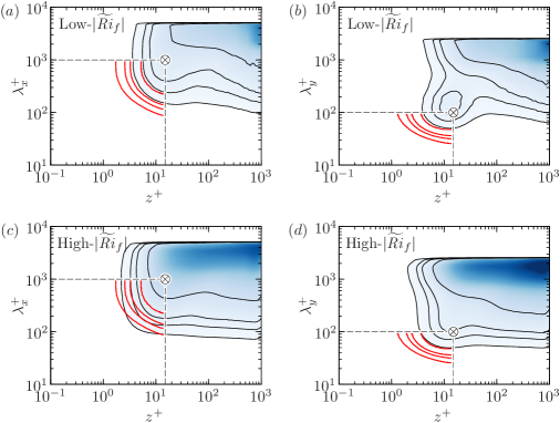
Figure 12: One-dimensional premultiplied conditional spectra of $u$ for $\mbox{{Ra}}=10^{9}$ shown as blue contours: ($a$,$c$) streamwise direction and ($b$,$d$) spanwise directions. ($a$,$b$) Low-$|\widetilde{\mbox{{Ri}}}_{f}|$ ($0<|\widetilde{\mbox{{Ri}}}_{f}|\leqslant 0.1$) spectra for higher-shear regions. ($c$,$d$) High-$|\widetilde{\mbox{{Ri}}}_{f}|$ ($|\widetilde{\mbox{{Ri}}}_{f}|>0.1$) spectra for lower-shear regions. The red contours are spectra from DNS of channel flow at $\Rey_{\tau}\approx 934$ (cf.  del Álamo et al., 2004), where only the contour levels in the near-wall region and shorter wavelengths are shown for clarity. The colormaps and contour levels are the same as figure 11. The $\otimes$ symbols denote the inner sites of channel flow spectra, which are respectively at ($z^{+}_{p}$,$\lambda_{x,p}^{+}$) $\approx$ ($15$,$1000$) and ($z^{+}_{p}$,$\lambda_{y,p}^{+}$) $\approx$ ($15$,$100$).

In order to obtain the local spectra of $u$, we first need to define the domain-lengths of a local streamwise-spanwise patch. In doing so, we restrict our analysis of the local spectra of $u$ to a patch that is associated with either low- or high-$|\mbox{{Ri}}_{f}|$. As a starting point, we choose the domain-lengths of the local patch as $2H\times H$ in the streamwise and spanwise directions. A patch is defined as locally shear-dominated if the plane-averaged value of $|\mbox{{Ri}}_{f}|$ in the local patch, which we denote by $|\widetilde{\mbox{{Ri}}}_{f}|$, is between $0$ and $0.1$, thus maintaining consistency with our criterion defined in § 4. From this definition, we obtain two conditionally averaged spectra for each direction: one for a (patch-averaged) higher-shear region, i.e.  low-$|\widetilde{\mbox{{Ri}}}_{f}|$, and another for a (patch-averaged) lower-shear region, i.e.  high-$|\widetilde{\mbox{{Ri}}}_{f}|$.

Next, since the local $u$ is not spatially periodic in the $x$- and $y$-directions, we introduce periodicity by appling a normalized Hann window $W(x_{i})=\sqrt{2/3}\,[1-\cos(2\pi n_{i}/N_{x_{i}})]$ (cf.  Chung & McKeon, 2010) in the $x$- and $y$-directions of the patch. This step is necessary in order to minimise spectral leakage when computing the spectra of a non-periodic local signal of $u$. Here, $N_{x_{i}}$ is the number of grid points in the $x_{i}$ direction and $n_{i}=1,\ldots,N_{x_{i}}$. This procedure is repeated at all wall-normal locations of the patch. The computed local spectra are then normalised by the local patch-averaged friction velocity $\widetilde{u}_{\tau}$ before averaging. Figure 12 shows the results for the conditionally averaged spectra at $\mbox{{Ra}}=10^{9}$, normalised by $\widetilde{u}_{\tau}^{2}$. For clarity, we compare our results with the channel flow spectra for $z^{+}\leqslant 15$, $\lambda_{x}^{+}\leqslant 1000$ and $\lambda_{y}^{+}\leqslant 100$.

Interestingly, when we closely inspect the contours of the low-$|\widetilde{\mbox{{Ri}}}_{f}|$ spectra of VC (figure 12$a$,$b$), we find that the shape of both streamwise and spanwise spectra have a relatively higher degree of resemblance with the spectra of channel flow compared to the contours in figure 11. The magnitude of the spectra of VC remains lower than the magnitude of the channel flow spectra. We also note the presence of a prominent near-wall peak in the spanwise conditional spectra of VC occurring at $z_{p,VC}^{+}\approx 15$ and $\lambda_{y,p,VC}^{+}\approx 150$ (see figure 12$b$), which is close to the inner site of the channel flow spectra. Additionally, the value of the peak spanwise wavelength in VC is consistent with the spanwise spacing of the streaks of approximately $100$ to $200$ viscous units observed in figure 3. These notable similarities between VC and turbulent channel flow imply that some form of the near-wall streaks is also locally present in VC, but the intensities of the streaks are dominated by the energy of considerably larger scales. From our dataset, we find that the near-wall similarities (both in spectra and flow visualisations) emerge at $\mbox{{Ra}}\gtrsim 2\times 10^{7}$. This suggests that for the present Ra-range, the VC flow is undergoing a transition to a regime where the boundary layers are increasingly influenced by stronger shear, which is consistent with our findings in the preceding sections.

For the conditionally averaged high-$|\widetilde{\mbox{{Ri}}}_{f}|$ spectra of VC (figure 12$c$,$d$), the shape of the contours retain characteristics that are similar to the unconditioned spectra of VC in figure 11. Namely, the shape of the streamwise spectra of VC differs from the streamwise spectra of channel flow whereas the spanwise contours retain the resemblance in shape but without a near-wall peak.

9 Summary and conclusion

The boundary layers in VC with Ra ranging between $10^{5}$ and $10^{9}$ and $\Pran$-value of $0.709$ are found to exhibit characteristics of a transition from a laminar-like scaling to a turbulent ultimate-regime-type behaviour.

Visually, the near-wall flow shows the emergence of two distinct regions with increasing Ra (figure 2). The first region appears streaky and correlates with higher-shear regions, whereas the second region is not streaky and correlates with lower-shear regions. The two regions are well-described by a flux Richardson number criterion where low-$|\mbox{{Ri}}_{f}|$ regions correspond to the streaky regions and high-$|\mbox{{Ri}}_{f}|$ regions correspond to the non-streaky regions (figure 5). With increasing Ra, the streaky low-$|\mbox{{Ri}}_{f}|$ regions occupy increasingly larger fractions of the wall-area (figure 6). This result suggests that the transition from the classical regime to the ultimate regime in VC manifests in the boundary layers as increasingly larger wall-area coverage of shear-dominated regions. Based on the trend of the increasing shear-dominated wall-areas, we estimate that at $\mbox{{Ra}}\gtrsim 10^{11}$ the boundary layers of VC are expected to be dominated by the streaky higher-shear structures for the $\Pran$-value of this study.

On further analysis, we find that the local statistics in the streaky low-$|\mbox{{Ri}}_{f}|$ regions exhibit trends that agree with turbulent boundary layer behaviour. In particular, the conditionally averaged mean temperature profiles of the low-$|\mbox{{Ri}}_{f}|$ regions show good agreement with the log-linear slope of the log-law of the wall for mean temperature (figure 7$d$). No log-linear trends are found in the low-$|\mbox{{Ri}}_{f}|$ conditional mean velocity profiles, both high-$|\mbox{{Ri}}_{f}|$ conditional mean velocity and temperature profiles, and the overall unconditioned mean velocity and temperature profiles.

In the streaky low-$|\mbox{{Ri}}_{f}|$ regions, the local Nusselt and Reynolds number follow an effective power scaling of $\mbox{{Nu}}_{l}\sim\mbox{{Ra}}^{0.37}$ and $\Rey_{l}\sim\mbox{{Ra}}^{0.41}$ (figure 8). The effective scaling exponent of $0.37$ for $\mbox{{Nu}}_{l}$ appears consistent with the logarithmically corrected $1/2$-power-law scaling predictions of the Nusselt number scaling relation in the ultimate regime. Additionally, the contributions from the Nusselt number in low-$|\mbox{{Ri}}_{f}|$ regions increasingly dominate the contributions from the high-$|\mbox{{Ri}}_{f}|$ regions (figure 9), which suggests that at sufficiently high Ra, the VC flow undergoes a transition to the ultimate regime presumably with $\mbox{{Nu}}\sim\mbox{{Ra}}^{0.37}$. In contrast, the effective scaling exponent of $0.41$ for $\Rey_{l}$ is lower than the $1/2$-power-law scaling predictions for the Reynolds number scaling relation in the ultimate regime. The lower exponent in the $\Rey_{l}$ scaling may be attributed to the local wind not being sufficiently strong to animate the turbulent boundary layers in the sense of Prandtl and von Kármán, as shown by the absence of a logarithmic-variation in the low-$|\mbox{{Ri}}_{f}|$ conditional mean velocity profiles (figure 7$c$). Indeed, investigations at much higher Ra are necessary in order to determine incipient logarithmic-variations in the mean velocity and temperature profiles, and how the local effective power-law scalings for Nusselt and Reynolds number in higher-shear regions are affected.

Finally, a comparison of our VC data and turbulent channel flow data at matched friction Reynolds number $\Rey_{\tau}$ reveals that the streaky regions in VC are reminiscent of the near-wall streaks in canonical wall-bounded flows. We find that a near-wall peak is present in the conditional low-$|\mbox{{Ri}}_{f}|$ spectra of VC in the spanwise direction (figure 12$b$). The corresponding wall-normal location is $z_{p,VC}^{+}\approx 15$ with a spanwise spacing of approximately 150 viscous length scales. This near-wall peak in the spectra of VC not only resembles the inner site of the spectra of turbulent channel flow, but the spanwise spacing of 150 viscous length scales is also consistent with the well-known spanwise Kline spacings of 100 viscous length scales in turbulent wall-bounded flows (see figure 3$b$,$d$).

Collectively, the results of the local logarithmic-variation in the mean temperature profile, higher exponent scaling for the Nusselt number and characteristics of the near-wall streaks suggest that the boundary layer in VC is undergoing a transition from the classical regime to an ultimate regime for the present Ra range. This transition is characterised by an increasing area coverage of shear-dominated patches in the near-wall region with increasing Ra and are consistent with the recent findings for Rayleigh–Bénard convection and Taylor–Couette flows.

Appendix A Sensitivity of $|\mbox{{Ri}}_{f}|$ threshold

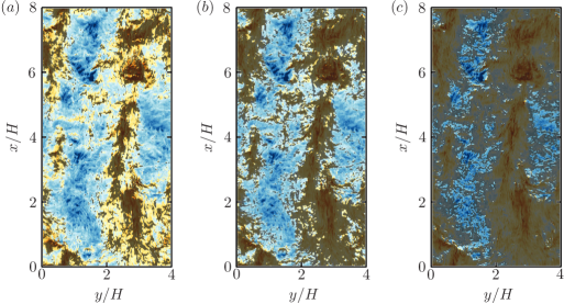
Figure 13: Plots of three Richardson number thresholds, shown as grey contours, overlayed on wall-parallel planes of streamwise velocity for $\mbox{{Ra}}=10^{9}$. The thresholds are ($a$) $0<|\mbox{{Ri}}_{f}|\leqslant 0.05$, ($b$) $0<|\mbox{{Ri}}_{f}|\leqslant 0.1$ (reproduced from figure 5$c$) and ($c$) $0<|\mbox{{Ri}}_{f}|\leqslant 0.5$. The velocity colormap is the same as in figure 2.

To illustrate the sensitivity of the $|\mbox{{Ri}}_{f}|$ threshold proposed in § 4, we plot the wall-area coverage for three threshold $|\mbox{{Ri}}_{f}|$-values for $\mbox{{Ra}}=10^{9}$ in figure 13. The shaded grey contours are the higher-shear regions-of-interest, $\rho$, and the values are $\rho\approx 0.28$, $0.58$ and $0.92$ for $0<|\mbox{{Ri}}_{f}|\leqslant 0.05$, $0<|\mbox{{Ri}}_{f}|\leqslant 0.1$ (used in this study) and $0<|\mbox{{Ri}}_{f}|\leqslant 0.5$. Note that the values of $\rho$ can also be calculated by integrating the area under the premultiplied PDF in figure 4($b$) for the corresponding Ra-value. From figure 13($c$), the grey contours encompass a larger area and include portions of the lower-shear regions, in blue; the local statistics in the higher-shear regions are therefore contaminated by laminar-like lower-shear regions. In contrast, the lower threshold values (figures 13$a$ and $b$) encompass smaller areas and only parts of the higher-shear regions, in red.

References

- Ahlers et al. (2012) Ahlers, G., Bodenschatz, E., Funfschilling, D., Grossmann, S., He, X., Lohse, D., Stevens, R. J. A. M. & Verzicco, R. 2012 Logarithmic temperature profiles in turbulent Rayleigh–Bénard convection. Phys. Rev. Lett. 109 (11), 114501.
- Ahlers et al. (2014) Ahlers, G., Bodenschatz, E. & He, X. 2014 Logarithmic temperature profiles of turbulent Rayleigh–Bénard convection in the classical and ultimate state for a Prandtl number of 0.8. J. Fluid Mech. 758, 436–467.
- Ahlers et al. (2009) Ahlers, G., Grossmann, S. & Lohse, D. 2009 Heat transfer and large scale dynamics in turbulent Rayleigh–Bénard convection. Rev. Mod. Phys. 81, 503–537.
- del Álamo et al. (2004) del Álamo, J. C., Jiménez, J., Zandonade, P. & Moser, R. D. 2004 Scaling of the energy spectra of turbulent channels. J. Fluid Mech. 500, 135–144.
- Businger et al. (1971) Businger, J. A., Wyngaard, J. C., Izumi, Y. & Bradley, E. F. 1971 Flux-profile relationships in the atmospheric surface layer. J. Atmos. Sci. 28 (2), 181–189.
- Chillà & Schumacher (2012) Chillà, F & Schumacher, J 2012 New perspectives in turbulent Rayleigh–Bénard convection. Eur. Phys. J. E 35 (7), 1–25.
- Chung & McKeon (2010) Chung, D & McKeon, BJ 2010 Large-eddy simulation of large-scale structures in long channel flow. J. Fluid Mech. 661, 341–364.
- Eriksson et al. (1998) Eriksson, J. G., Karlsson, R. I. & Persson, J 1998 An experimental study of a two-dimensional plane turbulent wall jet. Exp. Fluids 25 (1), 50–60.
- Grossmann & Lohse (2000) Grossmann, S. & Lohse, D. 2000 Scaling in thermal convection: a unifying theory. J. Fluid Mech. 407, 27–56.
- Grossmann & Lohse (2001) Grossmann, S. & Lohse, D. 2001 Thermal convection at large Prandtl numbers. Phys. Rev. Lett. 86, 3316–3319.
- Grossmann & Lohse (2002) Grossmann, S. & Lohse, D. 2002 Prandtl and Rayleigh number dependence of the Reynolds number in turbulent thermal convection. Phys. Rev. E 66 (1), 016305.
- Grossmann & Lohse (2004) Grossmann, S. & Lohse, D. 2004 Fluctuations in turbulent Rayleigh–Bénard convection: the role of plumes. Phys. Fluids 16, 4462–4472.
- Grossmann & Lohse (2011) Grossmann, S. & Lohse, D. 2011 Multiple scaling in the ultimate regime of thermal convection. Phys. Fluids 23 (4), 045108.
- Grossmann & Lohse (2012) Grossmann, S. & Lohse, D. 2012 Logarithmic temperature profiles in the ultimate regime of thermal convection. Phys. Fluids 24 (12), 125103.
- Grossmann et al. (2016) Grossmann, S., Lohse, D. & Sun, C. 2016 High-Reynolds number Taylor–Couette turbulence. Annu. Rev. Fluid Mech. 48, 53–80.
- He et al. (2012) He, X., Funfschilling, D., Nobach, H., Bodenschatz, E. & Ahlers, G. 2012 Transition to the ultimate state of turbulent Rayleigh–Bénard convections. Phys. Rev. Lett. 108 (2), 024502.
- Hughes & Griffiths (2008) Hughes, G. O. & Griffiths, R. W. 2008 Horizontal convection. Annu. Rev. Fluid Mech. 40, 185–208.
- Hutchins & Marusic (2007a) Hutchins, N. & Marusic, I. 2007a Evidence of very long meandering features in the logarithmic region of turbulent boundary layers. J. Fluid Mech. 579, 1–28.
- Hutchins & Marusic (2007b) Hutchins, N. & Marusic, I. 2007b Large-scale influences in near-wall turbulence. Philos. Trans. R. Soc. London, Ser. A 365 (1852), 647–664.
- Kline et al. (1967) Kline, S. J., Reynolds, W. C., Schraub, F. A. & Runstadler, P. W. 1967 The structure of turbulent boundary layers. J. Fluid Mech. 30 (04), 741–773.
- Landau & Lifshitz (1987) Landau, L. D. & Lifshitz, E. M. 1987 Fluid Mechanics, 2nd edn. Pergamon Press.
- Lohse & Xia (2010) Lohse, D. & Xia, K.-Q. 2010 Small-scale properties of turbulent Rayleigh–Bénard convection. Annu. Rev. Fluid Mech. 42, 335–364.
- Marusic et al. (2010) Marusic, I., McKeon, B. J., Monkewitz, P. A., Nagib, H. M., Smits, A. J. & Sreenivasan, K. R. 2010 Wall-bounded turbulent flows at high Reynolds numbers: Recent advances and key issues. Phys. Fluids 22 (6), 065103.
- Monin & Yaglom (2007) Monin, A. S. & Yaglom, A. M. 2007 Statistical Fluid Mechanics: Mechanics of Turbulence, , vol. 1. MIT Press.
- Ng et al. (2015) Ng, C. S., Ooi, A., Lohse, D. & Chung, D. 2015 Vertical natural convection: application of the unifying theory of thermal convection. J. Fluid Mech. 764, 349–361.
- Ostilla-Mónico et al. (2014) Ostilla-Mónico, R., van der Poel, E. P., Verzicco, R., Grossmann, S. & Lohse, D. 2014 Boundary layer dynamics at the transition between the classical and the ultimate regime of Taylor–Couette flow. Phys. Fluids 26 (1), 015114.
- Pallares et al. (2010) Pallares, J., Vernet, A., Ferre, J. A. & Grau, F. X. 2010 Turbulent large-scale structures in natural convection vertical channel flow. Int. J. Heat Mass Transfer 53, 4168–4175.
- van der Poel et al. (2015) van der Poel, E. P., Ostilla-Mónico, R., Verzicco, R., Grossmann, S. & Lohse, D. 2015 Logarithmic mean temperature profiles and their connection to plume emissions in turbulent Rayleigh–Bénard convection. Phys. Rev. Lett. 115 (15), 154501.
- Pope (2000) Pope, S. B. 2000 Turbulent Flows. Cambridge University Press.
- Scheel & Schumacher (2016) Scheel, J. D. & Schumacher, J. 2016 Global and local statistics in turbulent convection at low Prandtl numbers. J. Fluid Mech. 802, 147–173.
- Shang et al. (2003) Shang, X-D, Qiu, X-L, Tong, P & Xia, K-Q 2003 Measured local heat transport in turbulent Rayleigh–Bénard convection. Phys. Rev. Lett. 90 (7), 074501.
- Shang et al. (2008) Shang, X.-D., Tong, P. & Xia, K.-Q. 2008 Scaling of the local convective heat flux in turbulent Rayleigh–Bénard convection. Phys. Rev. Lett. 100 (24), 244503.
- Shishkina (2016) Shishkina, O. 2016 Momentum and heat transport scalings in laminar vertical convection. Phys. Rev. E 93 (5), 051102.
- Shishkina et al. (2016) Shishkina, O., Grossmann, S. & Lohse, D. 2016 Heat and momentum transport scalings in horizontal convection. Geophys. Res. Lett. .
- Shishkina & Horn (2016) Shishkina, O. & Horn, S. 2016 Thermal convection in inclined cylindrical containers. J. Fluid Mech. 790, R3.
- Smits et al. (2011) Smits, A. J., McKeon, B. J. & Marusic, I. 2011 High-Reynolds number wall turbulence. Annu. Rev. Fluid Mech. 43, 353–375.
- Turner (1979) Turner, J. S. 1979 Buoyancy effects in fluids. Cambridge University Press.
- Versteegh & Nieuwstadt (1999) Versteegh, T. A. M. & Nieuwstadt, F. T. M. 1999 A direct numerical simulation of natural convection between two infinite vertical differentially heated walls scaling laws and wall functions. Int. J. Heat Mass Transfer 42, 3673–3693.
- Wei & Ahlers (2014) Wei, P. & Ahlers, G. 2014 Logarithmic temperature profiles in the bulk of turbulent Rayleigh–Bénard convection for a Prandtl number of 12.3. J. Fluid Mech. 758, 809–830.
- Wygnanski et al. (1992) Wygnanski, I., Katz, Y. & Horev, E. 1992 On the applicability of various scaling laws to the turbulent wall jet. J. Fluid Mech. 234, 669–690.
- Yaglom (1979) Yaglom, A. M. 1979 Similarity laws for constant-pressure and pressure-gradient turbulent wall flows. Annu. Rev. Fluid Mech. 11 (1), 505–540.