A Guide to General-Purpose Approximate Bayesian Computation Software

1 Introduction

There are currently many programs available to conduct ABC analyses (see Table 1). However, most programs are specific to a particular problem, and the large majority for questions that typically arise in a population-genetics setting. These include programs to infer demographic histories (e.g. ONeSAMP , PopABC, msABC or DIYABC) , to infer F-statistics (ABC4F) or to infer parental contributions in an admixture event (2BAD). However, there exist also programs for phylogeographic inference (msBayes) , Systems Biology (ABC-SysBio) or the inference under stochastic differential equations (the MATLAB package abc-sde).

A major benefit of such specific programs is that a model parameterization suitable for simulation-based inference has already been worked out and a set of summary statistics informative for the problem identified. However, a particularly powerful aspect of ABC is its application to almost any inference problem and model, and we will thus focus here on general purpose ABC software designed to be helpful in a large array of ABC applications, either to conduct the whole analysis pipeline or at least specific parts of it.

Specifically, we will discuss two similar ABC pipelines, one provided through the command line program ABCtoolbox (version 2.0, Wegmann et al. (2010)), and the other by means of combining the two R packages abc (version 2.0, Csilléry et al. (2012)) and EasyABC (version 1.4, Jabot et al. (2013)). Both pipelines offer very similar features and build around a similar logic: 1) they both provide utilities to generate a large set of simulations using external simulation software that employs a variety of sampling algorithms, 2) they both offer algorithms to infer parameters from such a set of simulations, 3) they provide tools to conduct model choice from such sets of simulations performed under different models, and finally, 4) they both offer a series of functions to validate estimations as well as model choice. However, these pipelines differ in specific implementations of some algorithms, which we will outline below, as well as the general way users interact with them. The packages EasyABC and abc are used within the statistical software environment R and are hence well suited for people writing their simulation programs in R or for those familiar with the handling of data sets in this environment. In contrast, ABCtoolbox is written purely in C++ and run from the command line, resulting in generally faster execution and making it particularly well suited when command- line programs are used to conduct simulations or calculate summary statistics.

In the remainder of this chapter, we will walk the reader through the general usage of these two ABC pipelines. In order to give the reader a chance to replicate our analysis easily, we will use rather simple models and always give a detailed description of all settings used, along with all the code required to replicate the described analyses. We will begin with parameter inference, as we believe this is the step for which the programs discussed here will be used most often. However, we will also discuss how to use these pipelines to perform model choice, and how to conduct simulations using existing software.

Table 1: General and specific purpose ABC software.

Software	Purpose	Reference
ABCtoolbox	General	Wegmann et al. (2010)
abc	General	Csilléry et al. (2012)
ABC-EP	General	Barthelmé and Chopin (2011)
ABC_distrib	General	Beaumont et al. (2002)
ABCreg	General	Thornton (2009)
EasyABC	General	Jabot et al. (2013)
DIYABC	Population genetics	Cornuet et al. (2008)
msABC	Population genetics	Pavlidis et al. (2010)
ONeSAMP	Population genetics	Tallmon et al. (2008)
PopABC	Population genetics	Lopes et al. (2009)
2BAD	Population genetics	Bray et al. (2010)
ABC4F	Population genetics	Foll et al. (2008)
msBayes	Phylogeography	Hickerson et al. (2007)
ABC-SysBio	Systems Biology	Liepe et al. (2010)
abc-sde	Stochastic differential equations	Picchini (2014)

2 Toy models

We will introduce the usage of the program ABCtoolbox and the R packages EasyAbc and abc through their application to the problem of inferring the mean ($\mu$) and variance ($\sigma^{2}$) of a normal (Model A) and a uniform (Model B) distribution from a random sample. We will then further show how to use these ABC pipelines to distinguish between these models using model choice.

Using such simple models has two major benefits. First, it will allow us to compare the ABC estimates with those obtained from full likelihood solutions. Second, it is straightforward and quick to generate data under these models using just a few lines of code, for instance when using the free statistical programming language R, which we will do here. However, note that we will also discuss how to generate simulations with existing programs in Section 5.

2.1 Observed data and summary statistics

We will begin by generating a data set of 100 random samples under Model A (the normal distribution) for which we would like to infer parameters. This is readily done in R as follows:

⬇

sampleSize <- 100;

data.obs <- rnorm(sampleSize, mean=0, sd=1);

Note that for this test example we do know the true parameters $\theta=(\mu,\sigma^{2})$ that we want to estimate. This will allow us to test the accuracy of the estimation.

Next, we will define a function to calculate summary statistics both on the observed as well as simulated data sets. As summary statistics, we will use here the sample mean, variance and median, along with the smallest (min), largest (max) value, the range (max - min) and the first and third quartile (Q1 and Q3). A vector containing these summary statistics is readily generated in R using the following function:

⬇

calc.stats <- function (x){

S <- c(mean(x), var(x), median(x), range(x), max(x)-min(x),

quantile(x, probs=c(0.25, 0.75)));

names(S) <- c("mean", "var", "median", "min", "max", "range", "Q1", "Q3")

return(S);

}

This will now allow us to calculate these summary statistics on the observed data set (object data.obs), save them in the variable $S_{obs}$ (object S.obs) and to also save them in a file called normal.obs.

⬇

S.obs <- calc.stats(data.obs);

write.table(t(S.obs), file="normal.obs", quote=F, row.names=F);

While each run will produce different values, we provide the values we obtained and will use in the following in Table 2 to allow for the replication of all our results.

Table 2: Observed statistics of test data set

mean	var	median	min	max	range	Q1	Q3
0.102	1.14	0.0788	-2.02	3.16	5.18	-0.598	0.799

2.2 Generating simulations

We will next generate a large number (10,000) of simulations with parameter values drawn from prior distributions and calculate the associated summary statistics for each simulation. In order to allow for a direct comparison between the models, we will assume uniform prior distributions for the mean $\mu\sim U[-1,1]$ and variance $\sigma^{2}\sim U[0.1,4]$ for both models. We also set the internal random number seed generator equal to one so that the reader can reproduce exactly our results. Simulations for the normal model (Model A) are then generated as follows:

⬇

set.seed(1)

nsim <- 10000;

P.normal <- data.frame(mu=runif(nsim, min=-1, max=1), sigma2=runif(nsim, min=0.1 , max=4));

S.normal <- data.frame(matrix(data=0, ncol=length(S.obs), nrow=nsim));

names(S.normal) <- names(S.obs);

for ( i in 1:nsim ) {

y <- rnorm(sampleSize, mean = P.normal$mu[i], sd=sqrt(P.normal$sigma2[i]));

S.normal[i,] <- calc.stats(y);

}

write.table(cbind(P.normal, S.normal), file="simNorm.txt", quote=F, row.names=F);

Again, we saved the simulations also in a text file (simNorm.txt) in order to use them with ABCtoolbox. Note that ABCtoolbox requires the parameters and statistics in the same file, which is achieved by binding the data frames containing the parameters (P.normal) and statistics (S.normal) together using cbind().

Generating simulations under the uniform model (Model B) is achieved similarly. However, since the R function runif() requires the two limits $a,b$ of the uniform distribution, rather than the mean and variance, we need to calculate them from the parameters $\mu$ and $\sigma^{2}$ after each draw as $a=\mu-\sqrt{3\sigma^{2}}$ and $b=\mu+\sqrt{3\sigma^{2}}$, respectively.

⬇

nsim <- 10000;

P.unif <- data.frame(mu=runif(nsim, min=-1, max=1), sigma2=runif(nsim, min=0 , max=4));

S.unif <- data.frame(matrix(data=0, ncol=length(S.obs), nrow=nsim));

names(S.unif)<-names(S.obs);

for ( i in 1: nsim ) {

y <- runif(sampleSize, min=P.unif$mu[i]-sqrt(3*P.unif$sigma2[i]), max=P.unif$mu[i]+sqrt(3*P.unif$sigma2[i]));

S.unif[i,] <- calc.stats(y);

}

write.table(cbind(P.unif, S.unif), file="simUnif.txt", quote=F, row.names=F);

3 Parameter inference

The estimation of posterior distributions is straightforward with both ABCtoolbox and the R package abc. As a common feature, they both implement the basic rejection algorithm originally introduced by Tavaré et al. (1997) and Pritchard et al. (1999), but they differ in the post-sampling adjustment algorithms they offer. Specifically, the package abc implements the original post-sampling adjustment based on a local linear regression initially introduced by Beaumont et al. (2002), as well as an extension to non-linear models with heteroscedastic variance (Blum and François, 2010). In contrast, ABCtoolbox offers an implementation of the general linear model adjustment algorithm (ABC-GLM) introduced by Leuenberger and Wegmann (2010). In this section, we will discuss differences between these algorithms as well as how to use them in the present example.

3.1 Rejection Algorithm

abc

To start using abc, the package has first to be installed and loaded in R, which is done by the following two commands:

⬇

install.packages("abc");

library(abc);

To now conduct an ABC rejection on the data simulated under the normal model (Model A), simply use the function abc() with the argument method="rejection" and by specifying the tolerance to be applied.

⬇

rejection <- abc(S.obs,P.normal,S.normal,tol=0.01,method="rejection");

Here, S.obs, P.normal and S.normal refer to the vector of observed summary statistics $S_{obs}$ and the data frames containing the simulated parameters and summary statistics, respectively, as generated under Section 2. The additional argument tol specifies the fraction of simulations to be retained based on their distance to the observed summary statistics. A tolerance of $0.01$, for example, indicates that the posterior density will be estimated from the parameter values of the 1% of all simulations that produced summary statistics closest to the observed summary statistics based on an euclidean distance metric.

The package abc offers an internal plotting function hist.abc() to display posterior distributions. Since this function overloads the basic hist() function of R, it can be called on an abc object by simply typing:

⬇

hist(rejection);

Alternatively, it is also possible to use general R functions such as hist() or density() to plot posterior distributions. The results we obtained for the observed data shown above is plotted using density in Figure 1.

ABCtoolbox

In contrast to the R packages discussed here, the program ABCtoolbox is a program to be used from the command line, preferentially in a Unix/Linux environment. While it can be run from the Windows command prompt, it is recommend to use the cygwin Unix-like interface on a Windows computer to benefit from all features of ABCtoolbox.

ABCtoolbox accepts input settings both directly from the command line, as well as through an input file. A list of all arguments relevant for estimation and discussed in this chapter is provided in Table 3. To perform parameter estimation for the normal distribution example, for instance, the following input file may be used:

⬇

task estimate

simName simNorm.txt

obsName normal.obs

params 1-2

maxReadSims 10000

numRetained 100

writeRetained

maxCor 1.0

Here, the argument task is set to estimate in order to run ABCtoolbox in estimation mode. Then, the argument simName specifies the name of the file containing the performed simulations. This file is requested to contain the used model parameter values together with the associated statistics, the names of which are provided in the first line. Similarly, the file specified with the argument obsName should contain the summary statistics $S_{obs}$ calculated from the observed data, again with the first line of the file containing the names of the statistics and the second line the associated values. Using the argument params, ABCtoolbox is further told which columns of the simulation file contain the model parameters to be estimated. Note that the simulation file may contain an arbitrary number of additional columns that will be ignored if they are neither specified to be model parameters with the argument params nor summary statistics also present in the file with the observed summary statistics.

The additional required arguments maxReadSims and numRetained specify the maximum number of lines (simulations) that will be read from the simulation file, and the number of simulations to be retained in the rejection step, respectively. Finally, the argument maxCor specifies the maximal allowed correlation between summary statistics. If we also add the argument pruneCorrelatedStats then the analysis will be performed by using statistics that their pairwise correlation do not exceed the maxCor threshold . We will discuss the issues with correlated statistics below (section 4.3), but set this option here to 1 in order to include all statistics in the calculations and to avoid ABCtoolbox complaining about the presence of highly correlated statistics in our toy models.

To run ABCtoolbox with this input file (assuming it was saved under the name estimate.input), simply run in the command:

⬇

./ABCtoolbox estimate.input

Alternatively, the example can be run without using an input file by specifying the commands in the command line as:

⬇

./ABCtoolbox task=estimate simName=’*\dnormSimulated*’ obsName=’*\dnormObserved*’

params=1-2 maxReadSims=10000 numRetained=100 writeRetained maxCor=1.0

The output of such a run is found in a series of files, the names of which begin with a prefix that can be set with the argument outputPrefix, a tag referring to its content, and a number referring to the data set and model for which the estimation has been conducted. While an exhaustive list of all output filename tags discussed in this chapter is given in Table 4, we will focus here on the file with tag BestSimsParamStats, which contains the retained simulations and is used to plot the rejection posterior.

The posterior estimates for $\mu$ and $\sigma^{2}$ obtained from the ABC-rejection algorithm are readily plotted in R using the density() function.

⬇

par(mfrow=c(1,2))

ABCrej<-read.delim("ABC_GLM_model0_BestSimsParamStats_Obs0.txt",sep="\t");

plot(density(ABCrej$mu,from=-1,to=1),main=expression(mu));

plot(density(ABCrej$sigma2,from=0,to=4),main=expression(sigma^2));

The results we obtained for the observed data shown above are plotted using density in Figure 1.

3.2 Post-sampling adjustments

Posterior distributions estimated with the rejection algorithm tend to be much broader than the true posterior distributions. This is shown for the normal model in Figure 1, but has been observed generally and is due to the often relatively large distance thresholds leading to parameter values resulting in summary statistics rather distant from $S_{obs}$ to be accepted. Obviously, this loss of precision can be reduced by being more restrictive in accepting simulations, but this may require unrealistically computational efforts, particularly in more complex models.

An alternative is to correct for the effect of using large thresholds by exploiting the often simpler relationship between model parameters and summary statistics locally around the observed summary statistics. In a landmark paper, Beaumont et al. (2002) assume a linear relationship between model parameters and summary statistics locally among the retained simulations and proposed to use this relationship to project the parameter values of all retained parameter values to $S_{obs}$. More recently, Blum and François (2010) introduced an extension of this approach by fitting a non-linear, heteroscedastic model using neural networks. Both of these algorithms are implemented in the R package abc.

In contrast, ABCtoolbox offers an implementation of the ABC-GLM algorithm introduced by Leuenberger and Wegmann (2010) that estimates a local likelihood function instead of directly targeting the posterior distribution. While potentially slightly slower, this formulation is flexible in the choice of prior distributions and allows for model choice based on the marginal density. In practice, however, all mentioned post-sampling adjustment algorithms tend to give very similar results and the reader is advised to validate any estimation carefully in which these algorithms produce diverging estimates.

abc

The two post-sampling adjustments implemented in the R package abc are used by simply choosing the appropriate method when calling the abc() function. There are three different methods available: loclinear, ridge and neuralnet, which correspond, respectively, to the classic regression adjustment introduced by Beaumont et al. (2002), a version of this algorithm using a ridge regression to deal with extensive collinearity among statistics, and the non-linear, heteroscedastic regression proposed by Blum and François (2010). When using the loclinear method, if a warning appears regarding the collinearity of the design matrix then we recommend to use the ridge method instead.

The following commands will perform posterior estimation using these algorithms on the toy model introduced above.

⬇

regression <- abc(S.obs,P.normal,S.normal,tol=0.01,method="loclinear");

neural <- abc(S.obs,P.normal,S.normal,tol=0.01,method="neuralnet");

The built-in function hist() can then again be used to plot the estimated posterior distributions.

⬇

hist(regression);

hist(neural);

Another function provided by the package abc is plot.abc, which can be used to plot the densities of the estimated posterior distributions together with additional, informative plots such as the prior distribution, the distribution of euclidean distances, and the residuals of the regression. Since this function overloads the standard R function plot(), it is simply used as follows:

⬇

plot(regression,param=P.normal);

plot(neural,param=P.normal);

Alternatively, the estimated posterior distributions can also be plotted using the R function density. For that purpose, one has to access specific elements of the object returned by the abc() function, namely the projected model parameter values as adj.values as well as their weights weights. The following R commands, for instance, plot the posterior densities obtained via the regression and neural network adjustment for $\mu$:

⬇

plot(density(regression$adj.values[,1], weights=regression$weights/sum(regression$weights)),main=expression(mu));

plot(density(neural$adj.values[,2], weights=neural$weights/sum(neural$weights)),main=expression(sigma^2));

Posterior distributions plotted using these functions are compared to those obtained through other methods in Figure 1. Note that the object returned also contains the retained model parameter values in the element unadj.values that can be used to plot the rejection posterior distribution.

⬇

plot(density(regression$unadj.values[,1]),main=expression(mu));

plot(density(regression$unadj.values[,2]),main=expression(sigma^2));

ABCtoolbox

When running ABCtoolbox in estimation mode, the ABC-GLM adjustment introduced by Leuenberger and Wegmann (2010) is performed automatically and the results available in the output file with tag MarginalPosteriorDensities. To plot the posterior estimates in R, simply load that file and use the function density.

⬇

par(mfrow=c(1,2))

ABCglm <- read.delim("ABC_GLM_model0_MarginalPosteriorDensities_Obs0.txt");

plot(ABCglm$mu,ABCglm$mu.density,type="l");

plot(ABCglm$sigma2,ABCglm$sigma2.density,type="l");

Table 3: ABCtoolbox settings for estimation.

Setting type	Setting	Description
Basic	task	Task to be performed. Possible options are: simulate, estimate, findStatsModelChoice
	estimationType	Standard estimation performs the GLM approach Leuenberger and Wegmann (2010).
	params	Specify the parameter columns in the file that contains the simulations.
	simName	File containing simulations.
	obsName	File containing observed summary statistics.
	numRetained	No. of simulations to retain.
	maxReadSims	Maximum number of read simulations.
	pruneCorrelatedStats	Remove statistics that are correlated, possible options 0 (retain) or 1 (remove).
	maxCor	Maximum acceptaple correlation coefficient between statistics.
	outputPrefix	Prefix for output files.
	writeRetained	Indicate whether to write retained simulations which can be used to obtain ABC rejection posteriors.
	standardizeStats	Standardize statistics.
Validation	obsPValue	The number of retained data sets for testing how well the inferred GLM model fits the observed data in multidimensional space (section 3.4.1).
	tukeyPValue	The number of retained data sets for performing the Tukey test (section 3.4.1).
	modelChoiceValidation	The number of cross-validation replicates for validating model choice (section 4.2).
	randomValidation	The number of cross-validation replicates for random parameter validation (section 3.4.3).
	retainedValidation	The number of cross-validation replicates for retained parameter validation (section 3.4.3).
Posterior density	posteriorDensityPoints	Number of points to estimate posterior density.
	diracPeakWidth	Smoothing parameter for posterior densities.
	jointPosteriors	Comma separated list of parameters for which the joint posterior is to be evaluated (section 3.3).
	jointPosteriorDensityPoints	No. of points to evaluate joint posterior (section 3.3).

Table 4: ABCtoolbox estimation output files.

File type	File tag	Content
Basic	MarginalPosteriorCharacteristics	Characteristics of marginal posterior distributions (e.g., mode, mean, quantiles).
	BestSimsParamStats	Retained simulations from ABC-rejection.
	MarginalPosteriorDensities	GLM-adjusted marginal posterior densities.
	jointPosterior	GLM-adjusted joint posterior estimates.
	modelFit	Model choice results including bayes factors and posterior support for compared models.
Parameter validation	RandomValidation	Results from random validation.
	RetainedValidation	Results from retained validation.
Model choice validation	modelChoiceValidation	Results for model choice validation.

3.3 Multidimensional posteriors

abc

Apart from marginal posterior distributions, both the R package abc as well as ABCtoolbox are capable of estimating multidimensional posterior distributions. In the case of abc, however, the posterior densities have to be estimated using standard functions of R such as kde2d() for two-dimensional posterior distributions. In our toy model, for instance, using

⬇

posterior2d <- kde2d(regression$adj.values[,1],regression$adj.values[,2],n=100);

contour(posterior2d,xlab=expression(mu),ylab=expression(sigma^2));

where, regression$adj.values[,1] represents the projected model parameter values for $\mu$, regression$adj.values[,2] represents the projected model parameter values for $\sigma^{2}$, and n=100 specifies the number of marginal grid points to be used for the density estimation. These R commands will produce a plot similar to the one in figure 1C.

ABCtoolbox

To generate multidimensional posterior densities on a grid, simply add the argument jointPosteriors, followed by the names of the model parameters for which the multidimensional posterior distribution is to be estimated. In addition, the number of marginal grid points has to be specified using jointPosteriorDensityPoints. The joint posterior estimates for the parameters $\mu$ and $\sigma^{2}$ of the normal distribution model, for instance, is thus estimated by simply running ABCtoolbox with a modified estimate.input input file that contains these two additional lines:

⬇

jointPosteriors mu,sigma2

jointPosteriorDensityPoints 100

Note that the total number of grid points grows exponentially with the dimensionality. In this above example, the density will be evaluated at $100\times 100=10^{4}$ positions. Running such a command for a four dimensional posterior will already result in $10^{8}$ positions at which the density has to be estimated.

When running ABCtoolbox with the additional arguments jointPosteriors and jointPosterior DensityPoints, the posterior density at each grid point will be written to an output file with tag jointPosterior. The resulting joint posterior of $\mu$ and $\sigma^{2}$ can then be plotted in R using the function contour().

⬇

plot2D <- read.delim("ABC_GLM_model0_jointPosterior_1_2_Obs0.txt");

x <- unique(plot2D$mu);S.unif$var

y <- unique(plot2D$sigma2);

z_density <- matrix(data=plot2D$density,nrow=length(x),ncol=length(y),byrow=F);

contour(x,y,z_density,xlab=expression(mu),ylab=expression(sigma^2));

Since densities may be hard to interpret, ABCtoolbox also calculates and prints the smallest high posterior density interval (HDI) including each grid point to the same output file. The HDI corresponds to a posterior credible interval in the multidimensional parameter space and hence allows the generation of contour plots where contour lines indicate posterior credible intervals as follows:

⬇

z_HPD <- matrix(data=plot2D$HDI,nrow=length(x),ncol=length(y),byrow=F);

contour(x,y,z_HPD,xlab=expression(mu),ylab=expression(sigma^2));

The two dimensional posterior distribution we obtained this way for the normal distribution example is given in Figure 1C.

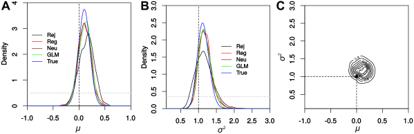
Figure 1: Posterior densities for the mean (A) and variance (B) parameters of the normal distribution model produced by a variety of methods. Dashed grey lines indicate prior densities. (C) Joint posterior density for $\mu$ and $\sigma^{2}$ produced with ABCtoolbox. Dashed black lines indicate true parameter values for all panels.

Note that using a grid evaluation is not suitable to estimate multidimensional densities in high dimensions as the total number of grid points grows exponentially with the dimensionality. In this above example, the density will be evaluated at $100\times 100=10^{4}$ positions. Running such a command for a four dimensional posterior will already result in $10^{8}$ positions at which the density has to be estimated. An alternative is to generate samples from the joint posterior distribution from which densities are estimated using kernel estimators. To generate samples from high-dimensional posterior distributions after post-sampling adjustment, ABCtoolbox also implements an MCMC algorithm. While we will not discuss that algorithm here, we refer the user to the manual of ABCtoolbox for more details.

3.4 Validation of parameter estimation

3.4.1 Using a wrong model

An essential first validation step is to check whether the observed statistics can be reproduced by the examined model. A failure of the model to reproduce some of the statistics may indicate that a model is either not reflecting reality close enough, or that inappropriate prior distributions have been used (e.g., too narrow distributions). More importantly, all post-sampling adjustments assume that the model fitted to the model parameters and summary statistics can be used to either accurately project retained simulations to $S_{obs}$ (the methods implemented in abc), or is an accurate description of the likelihood of $S_{obs}$ with the parameter range of the retained simulations (the method implemented in ABCtoolbox). A violation of these assumptions leads to an extrapolation to an area of the summary statistics space for which no samples have been obtained, and is hence is prone to biased inference.

Checking if the observed summary statistics $S_{obs}$ are within the range of summary statistics generated by the model is, however, a bit tricky in higher dimensions. For instance, consider the marginal summary statistics distributions shown in Figure 2 for the normal and uniform toy models, respectively. These distributions were plotted in R using the density() function directly from the simulated data.

⬇

plot(density(S.normal$var), col=’black’);

lines(density(S.unif$var), col=’grey’);

abline(v=S.obs[2])

These plots suggest that both summary statistics are readily generated by both models. However, a mismatch might manifest when looking at combinations of summary statistics. To check this we can plot two-dimensional distributions of pairs of summary statistics using the R functions kde2d and contour.

⬇

d <- kde2d(S.unif$var, S.unif$range, n=100);

contour(d$x, d$y, d$z);

As is shown in the rightmost panel in Figure 2, the combination of the two observed summary statistics variance and range can indeed not be reproduced by the uniform model. However, this fact is not visible when looking at marginal densities only.

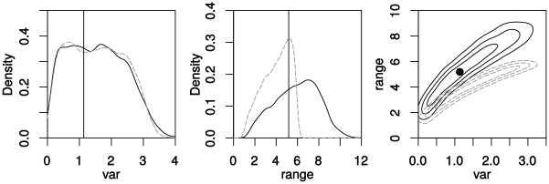
Figure 2: The distributions of simulated versus observed statistics variance (left panel) and range (middle panel) and their joint distribution (right panel) for the normal (black) and uniform (grey) distribution models. Observed data is shown with a black vertical line in the left and middle panels and with a black dot in the right panel.

ABCtoolbox

Since visual inspection is only fruitful for a limited number of dimensions, ABCtoolbox offers two statistical tests for assessing whether a given model can reproduce the observed data $S_{obs}$ in the multidimensional statistics space. The first test compares the marginal density (also called marginal likelihood) of the observed data to the marginal density of the retained simulations. The fraction of retained simulations with smaller or equal marginal density than the observed data is then provided as the marginal density P-value where small values indicate a poor fit of the model to the observed data.

The second test evaluates how central the observed data lies within the multidimensional cloud of retained simulations by reporting the fraction of retained simulations with smaller or equal Tukey depth than the observed data as the Tukey P-value (Cuesta-Albertos and Nieto-Reyes (2008); Adrion et al. (2014)). The Tukey depth is a common measure of centrality analogous to the median in one dimension and is calculated by ABCtoolbox for a retained simulation (or the observed data) as the smallest fraction of retained simulations which can be separated from the rest of the simulations using a hyper plane through the chosen simulation (or the observed data). Again, a low Tukey P-value indicates a poor fit of the model since the observed data appears to be at the periphery of the retained cloud. However, note that the opposite is not necessarily true. Indeed, even a poor model (e.g. a model producing summary statistics at random) may be capable of generating a cloud of summary statistics surrounding $S_{obs}$, and will thus pass both tests.

To perform these tests, simply call ABCtoolbox with the arguments marDensPValue and tukeyPValue, where each of them indicates the number of retained simulations to be used when calculating the respective P-value. When adding the following two lines to the input file estimate.input, for instance, ABCtoolbox will use 1,000 retained simulations to evaluate the P-values.

⬇

marDensPValue 1000

tukeyPValue 1000

The results we obtained for these tests for our toy models is shown in Table 5. As expected from the visual inspection in Figure 2, the uniform model is not capable of reproducing the observed data and hence fails both tests.

Table 5: Observed P-value and Tukey P-value results for normal distribution example

Model	marginal density	marginal density P-Value	Tukey Depth	Tukey P-Value
1	1158.75	0.098	0.13	0.96
2	$4.16\times 10^{-12}$	0	0	0

3.4.2 Cross-validation / Accuracy of point estimates

The accuracy of posterior point estimates is generally assessed by estimating the parameters for data sets for which the true parameter values are known. This is readily done in an ABC setting as a leave-one-out test in which one of the provided simulations is randomly chosen and all other are used to infer the parameter estimates for this data (often called “pseudo-observed” data). The inferred posterior point estimates such as the maximum a posteriori (MAP or posterior mode), the posterior mean or the posterior median are then plotted against the parameter values used to generate the data (referred to as the “true parameters”). This process (also called cross-validation) is then repeated for many “pseudo-observed” data sets to obtain a general measure of accuracy. The procedure may also be repeated to test specific ABC settings such as the effect of the choice of tolerance or the number of available simulations.

abc

To use this cross-validation algorithm with the R package abc, simply call the function cv4abc() with the arguments matching those of the estimation plus the additional argument nval, which specifies how many pseudo-observed data sets are to be used. However, note that the observed data does not have to be provided, as it is not used in cross validation. The following code, for instance, will conduct cross validation on the normal distribution example for the neural network estimation algorithm based on 100 individual pseudo-observed data sets.

⬇

cv.neural <- cv4abc(P.normal, S.normal, tols=0.1, statistic="mode",method="neuralnet", nval=100);

Such a call will return an object containing both the true parameter values (element true) as well as the estimated parameter values (element estim), which can be used to estimate correlations among them and plot for visual inspection. A plot such as the one shown in Figure 3 is generated by

⬇

plot(cv.neural);

ABCtoolbox

ABCtoolbox offers two flavors of this cross-validation algorithm: either by picking simulations randomly, or by picking simulations only among those that were retained. The former, which is invoked through the argument randomValidation, corresponds to picking parameter values from the prior distribution and is thus informative above the overall accuracy of the ABC estimation under the chosen model. The latter, which is invoked using the argument retainedValidation, is informative about the accuracy of the estimation for the parameter space leading to similar data as the one observed.

⬇

task estimate

simName simNorm.txt

obsName normal.obs

params 1-2

maxReadSims 10000

numRetained 1000

maxCor 1.0

randomValidation 1000

retainedValidation 1000

When running ABCtoolbox with one or both of those arguments, an additional output file with tag randomValidation or retainedValidation is generated that contains the true parameter values along with a series of posterior point estimates for each parameter, namely the MAP (or mode) as well as the posterior mean and median. This file can then be loaded into R to generate plots such as those shown in Figure 3 as follows:

Figure 3: Parameter validation using different methods. The estimated posterior mode for mean and variance is plotted against the true values.

⬇

Random_validation <- read.delim("ABC_GLM_model0_RandomValidation.txt");

Retained_validation <- read.delim("ABC_GLM_model0_RetainedValidation_Obs0.txt");

plot(Random_validation$mu, Random_validation$mu_mode);

plot(Retained_validation$mu, Retained_validation$mu_mode);

3.4.3 Checking for biased posteriors

Pseudo-observed data sets can be used equally to detect potential biases in the marginal posterior distributions. If the posterior distributions of a parameter were unbiased, the position of the true parameters across many replicates must be given by the posterior densities. We proposed to test this directly using the probability integral transform test (PIT histogram, or coverage property) Wegmann et al. (2009); Prangle et al. (2014). This is done by recording the position of the true parameter value in the cumulative posterior distribution (the posterior quantile) for each pseudo-observed data set. In case posteriors were unbiased, these posterior quantiles must be uniformly distributed between 0 and 1. Similarly, the smallest high posterior density intervals (HDI) containing the true parameter value must be distributed uniformly.

ABCtoolbox

The procedure for this is the same as the one described in section 3.4.2. The same output file will contain information that allows us to check for biased posteriors. For instance, the output from these analyses can be used to determine whether the posterior quantiles and HDI are uniformly distributed either by visual inspection or by performing a statistical test such as the Kolmogorov-Smirnov test:

⬇

hist(Random_validation$mu_HDI)

ks.test(Random_validation$mu_HDI,"punif")

The result of the random and retained validation analyses for the normal distribution example can be seen in Figure 4A and Figure 4B, respectively.

Figure 4: Parameter validation testing uniformity of the distribution of posterior quantiles and HDI when using random (A) and retained (B) simulations.

4 Model choice

While model choice is commonly used in Bayesian statistics, it is contentious in an ABC setting due to the problem that even summary statistics sufficient for both models may lead to biased inferences (Didelot et al., 2011; Robert et al., 2011). Nonetheless, ABC model choice has been used successfully in practice and both ABC pipelines discussed here offer algorithms to conduct model choice when simulations from multiple models are available. However, the user is advised to validate any ABC model choice carefully and we will discuss here tools provided by the R package abc as well as ABCtoolbox to aid in that crucial step.

4.1 Inferring Bayes Factors

Bayesian model choice relies on the estimation of model posterior probabilities or Bayes factors (the ratios of posterior probabilities of competeing models). In standard Bayesian statistics, these are estimated from the marginal densities (or marginal likelihood) of the compared models, where the marginal density of model $i$ is defined as the integral of the likelihood function, weighted by the prior distribution:

$$\mathbb{P}(M_{i}|D)=\int\mathbb{P}(D|\theta_{i},M_{i})\mathbb{P}(\theta_{i}|M_{i})d\theta_{i}.$$

Importantly, the marginal density is thus affected by the choice of prior distribution, and hence what is evaluated in a Bayesian setting is thus the combination of a stochastic model and the prior destribution specified on its parameters.

In case the likelihood function is not available for analytical evaluation, both posterior probabilities and Bayes factors can be estimated using ABC. The algorithm implemented in ABCtoolbox, for instance, fits a likelihood model to the retained data, and then uses this model to analytically calculate the marginal density for each model. In contrast, the algorithms available in the R package abc use the fact that the marginal density is proportional to the fraction of simulations that resulted in simulations close to the observed data $S_{obs}$ when the simulations are generated according to the prior distribution. The posterior probabilities of the different models are thus estimated from the relative number of simulations being close to $S_{obs}$ either from direct counting or through a regression adjustment similar to parameter inference. Note that it is crucial for both algorithms that the exact same summary statistics have been calculated under both models.

To illustrate the model choice algorithms implemented, we will attempt to estimate which of the two toy models introduced above (the normal and uniform model) was used to generate the observed data. We refer the reader to section 2 for more details on those models.

abc

In order to conduct model choice with abc, the summary statistics of all models have to be concatenated into a single data frame or matrix. In addition, a vector indicating for each simulation the model under which it has been generated has to be created. For our toy models, this is simply achieved as follows:

⬇

allSimulations <- rbind(S.normal,S.unif);

index <- c(rep("norm",dim(S.normal)[1]),rep("unif",dim(S.unif)[1]));

The actual model choice is then conducted using the function postpr, which takes as arguments the observed summary statistics $S_{obs}$, the object containing the summary statistics for all models, and the index vector. In addition, the tolerance for the rejection step as well as the method for estimating Bayes factors has to be provided. In total, abc offers three such methods. The simplest is the the method rejection, which estimates posterior probabilities of the different models directly from the relative proportions of accepted simulations. The two other methods, mnlogistic and neuralnet attempt to correct for the often large tolerance values by estimating the relative densities of retained simulations at $S_{obs}$ using either a multinomial logistic regression Beaumont (2008); Fagundes et al. (2007) or neural networks François and Guillaume (2011), respectively.

The following command will run model choice using the neuralnet method on our toy models and, using the function summary(), print the results to screen in a nice format.

⬇

model.choice <- postpr(S.obs, index=index, sumstat=allSimulations, tol=0.1, method="neuralnet");

summary(model.choice);

The results for our toy models is shown in Table 6. As is expected from the observation that the uniform model fails to reproduce the observed summary statistics, the preferred model for this data is the normal model. However, note that the results for the rejection method, which is also run by default when performing a mnlogistic or neuralnet estimation, is much less clear due to the relatively large tolerance applied here.

Table 6: Results of model choice on toy models

	Posterior Probability			Bayes Factor
Model	Normal	Uniform		Normal vs. Uniform
abc (rejection)	0.65	0.395		1.53
abc (neuralnet)	1.00	0.00		$1.1\times 10^{6}$
ABCtoolbox (GLM)	1.00	$9.79\times 10^{-13}$		$9.79\times 10^{13}$

ABCtoolbox

To perform model choice with ABCtoolbox, simply provide the arguments simName and params for multiple models using semicolons. To run model choice on our toy models, for instance, the input file estimate.input provided abode is modified as follows:

⬇

task estimate

simName simNorm.txt;simUnif.txt

obsName normal.obs

params 1-2;1-2

maxReadSims 10000

numRetained 1000

maxCor 1.0

When running ABCtoolbox with such an input file, an additional file with tag modelFit is generated. This file contains the marginal densities, Bayes factors and posterior probabilities for each model. The results from this file obtained for our toy models is shown in Table 6, clearly indicating that the normal model is a much better fit.

4.2 Model choice validation

As was shown recently, model choice conducted with ABC may lead to biased or even wrong posterior probabilities, even if the summary statistics are sufficient for all models compared (see Robert et al. (2011)). Consider two models ${\cal M}_{1}$ and ${\cal M}_{2}$ of shared parameters $\theta$. If a set of summary statistics $S$ was sufficient for both models, then the likelihood of the summary statistics and the likelihood of the full data are proportional for both models

$$\mathbb{P}(D|\theta,{\cal M}_{1}) =c_{1}\mathbb{P}(S|\theta,{\cal M}_{1})$$

$$\mathbb{P}(D|\theta,{\cal M}_{2}) =c_{2}\mathbb{P}(S|\theta,{\cal M}_{2})$$

However, there is no guarantee that the two proportionality constants $c_{1}$ and $c_{2}$ are identical, which leads to the Bayes factors that are off by $c_{1}/c_{2}$. Therefore, careful validation is a key and compulsory step of any ABC model choice analysis. An initial first test may be to evaluate the power of choosing the correct model by means of pseudo-observed data sets. Such a cross-validation, which is offered by both abc as well as ABCtoolbox, simply picks random simulations among those provided from both models, conducts model choice, and records how frequently the correct model was preferred. In addition, ABCtoolbox provides means to test for biases in the obtained posterior probabilities by comparing the ABC posterior probability (termed $p_{ABC}$) against those empirically expected ($p_{empirical}$) (Peter et al., 2010).

abc

The R package abc contains the function cv4postpr to conduct cross-validation for model choice. This function randomly picks one simulation from the file containing all simulations, performs model choice using the chosen simulation as pseudo-observed data, and records which model obtained the highest posterior probability. This is then repeated many times to determine the confusion matrix. As an example, consider the following call to cv4postpr to conduct 100 such replicates on our toy models using the index vector created above. To then print the confusion matrix, one may use the function summary() and to obtain a graphical representation the built in plot() function as follows.

⬇

cv.model.choice <- cv4postpr(index,allSimulations, nval=100, tols=0.1, method="neuralnet")

summary(cv.model.choice);

plot(cv.model.choice);

ABCtoolbox

To perform model choice validation with ABCtoolbox, simply add the argument modelChoiceValidation followed by the number of pseudo-observed data sets to be used to the estimation file. To use 1000 pseudo-observed data sets, for instance, you may add the following line to the input file:

⬇

modelChoiceValidation 1000

ABCtoolbox will then perform cross validation and write the results to two different files. The first has the tag confusionMatrix containing the confusion matrix (fraction of correctly and incorrectly inferred models) as well as statistics calculated from it. For the toy model, for instance, we learn from this file that the normal model is correctly identified from data generated under that model in $>99\%$ of the cases.

The second file with tag modelChoiceValidation contains the raw results from the model choice validation and can be used for a more detailed validation analyses. For instance, we have recently proposed to compare the estimated model posterior probabilities with the empirical ones, an analysis that can reveal biases in ABC model choice (Peter et al., 2010; Chu et al., 2013). The basic logic of this analysis is that among all pseudo-observed data sets that resulted in an ABC posterior probability $p_{ABC}=x$ in favor of, say, model 1, a fraction $x$ should have been generated under model 1. To test for this, data sets are binned according to their ABC posterior probabilities $p_{ABC}$ and the empirical posterior probabilities $p_{empirical}$ are then estimated as the fraction of simulations within each bin that were indeed generated with model 1.

The ABCtoolbox package includes the Rscript Make_Model_choice_power_plot.r to conduct this analysis and to produce the plot shown in Figure 5. For our toy models it appears that there is a slight bias towards the normal model. This is evident from the fact that when $p_{ABC}=0.5$, the data sets were actually generated from the uniform model in about $70\%$ of the cases. However, among the data sets that resulted in very high $p_{ABC}$ $(\geq 0.99)$, the vast majority was generated under that model. Therefore, we have high confidence in the model choice results of our observed data, which produced $\geq 0.99$ posterior probability support for the normal distribution model (Table 6).

Figure 5: Posterior probability for normal and uniform distribution models estimated by ABCtoolbox ($p_{ABC}$) versus an empirical estimate of the same probability through simulation ($p_{empirical}$).

4.3 Choosing summary statistics

4.3.1 Statistics for parameter inference

The choice of summary statistics is crucial in any ABC inference in that too few summary statistics are likely to miss out on important information and too many introducing harmful noise to the estimation (Wegmann et al., 2009; Beaumont, 2008; Blum et al., 2013). To date, many methods have been proposed to choose informative summary statistics from a larger set (see Blum et al. (2013) for a review), but we will focus here on those available through the ABCtoolbox package, in particular the use of linear combinations of summary statistics.

The use of such linear combinations was first introduced by Wegmann et al. (2009), who proposed to find them by means of Partial Least Squares (PLS) regression. Broadly speaking, PLS is similar in spirit to a Principal Component Analysis (PCA), but instead of finding linear combinations that maximize the variance explained in the summary statistics space, PLS components are chosen such that they maximize the product of the variance among summary statistics and the covariance between parameters and statistics (Tenenhaus et al., 1995). Recently, alternative means of finding linear combinations of summary statistics have been proposed, such as through boosting (Aeschbacher et al., 2012a) or by regressing summary statistics on to posterior means inferred from an initial set of simulations (Fearnhead and Prangle, 2012).

While all these methods are readily used with ABCtoolbox once the linear combinations have been found, we will illustrate the usage of this functionality based on the PLS approach, which is easy to implemevR-package ’pls’. In fact, the ABCtoolbox package provides an R-script to perform this analysis taking as input the simulations file (simNorm.txt). Performing a PLS analysis on the simulations from the normal distribution example reveals that 2 PLS components are sufficient for explaining the variance of the parameters of the normal distribution (Figure 6). This result is expected since the mean of a sample and the mean and variance of a sample are sufficient statistics for estimating, respectively, the mean and variance parameters of a normal distribution.

Figure 6: Number of PLS components versus root mean square error of prediction (RMSEP) for the normal distribution model.

Any definition of linear combinations resulting from such a PLS or any other approach can then be used to transform the statistics of a set of simulations and the observed data using ABCtoolbox, and then used in parameter inference. The PLS R-script mentioned above, for instance, writes the resulting PLS components to the file PLSdef.txt, which is then provided to ABCtoolbox and run in the transform mode as follows:

⬇

./ABCtoolbox task=transform linearComb=PLSdef.txt input=’*\dnormSimulated*’ output=simNorm.pls numLinearComb=2

./ABCtoolbox task=transform linearComb=PLSdef.txt input=normal.obs output=normal.obs.pls numLinearComb=2

Note that while we provided all arguments to ABCtoolbox on the command line, they may equally well be given in an input file. Using the transformed summary statistics in the estimation step is then straightforward: simply provide the transformed files using the arguments simName and obsName.As mentioned above, using alternative ways to find linear combinations is compatible with ABCtoolbox, as long as the linear combinations can be written in a definition file as the one created by the PLS script. Alternatively, the statistics may also be transformed with different software and then provided to ABCtoolbox (or the R package abc) for the estimation step.

One issue with using linear combinations of summary statistics is that information that arises from non-linear combinations of statistics are not taken into account. In such situations, it may be beneficial to increase the summary statistics space through combinations of summary statistics before finding linear combinations (Aeschbacher et al., 2012b). As outlined with an example in section 5.3, ABCtoolbox has an option (doBoosting) to also generate all pairwise products of summary statistics when generating simulations for this purpose.

4.3.2 Statistics for model choice

Finding appropriate combinations of statistics for model choice is particularly tricky. Just as for parameter inference, too few statistics may fail to capture important information, while too many are likely adding non-informative noise leading to large estimation variance and potentially a bias. Unfortunately, the methods introduced above for finding good summary statistics for parameter inference are not readily extended to the problem of model choice. If one aims for using linear combinations, the most obvious choice is Linear Discriminant Analysis (LDA), as was recently proposed by Estoup et al. (2012). To use LDA for model choice with the programs discussed here is similar to the use of linear combinations for parameter inference in that the summary statistics of the observed and simulated data have to be transformed as explained in section 4.3.1 before running either ABCtoolbox or the R package abc to perform model choice.

As an alternative to LDA, ABCtoolbox offers a greedy search algorithm to identify the combination of statistics having the largest power to discriminate between models. This search is done iteratively, by firstly evaluating the power of each single statistic and then adding additional statistics until no increase in power is observed. To perform this type of analysis, ABCtoolbox has to be run in the findStatsModelChoice mode and by providing the simulation files for at least two models, as well as the parameters required to perform the estimation. In addition, and using the argument modelChoiceValidation, one also needs to specify the number of simulations to be used as pseudo-observed data in each iteration to evaluate the power. As an example, consider the following input file for performing this type of analysis to find summary statistics appropriate for contrasting the normal versus uniform distribution toy models. We have added argument maxCorSSFinder and set it equal to one in order to include combinations of statistics that are highly correlated in the greedy search. A lower threshold might be apporpirate if many summary statistics are used in order to speed up the search.

⬇

task findStatsModelChoice

simName simNorm.txt;simUnif.txt

obsName simple.obs

maxCor 1.0

maxCorSSFinder 1.0

params 1-2;1-2

numRetained 1000

maxReadSims 10000

outputPrefix ABC_searchStats

modelChoiceValidation 1000

The results of this analysis are written to a file with tag searchStatsgreedySearch. Part of this file is shown in Table 7. As shown there, the power to distinguish between these models is very high for multiple sets of summary statistics. Generally, it is recommended to choose the smallest among all sets with highest power, which would be the set consisting of the statistics var and range. As is shown in Figure 2, the two-dimensional distribution of these two statistics is indeed rather different between the models.

Table 7: Combinations of statistics sorted by estimated power to distinguish models.

Rank	Power	Largest Pairwise Correlation	No.statistics	Statistics
1	1	0.966	3	mean,var,range
6	0.999	0.966	2	var,range
82	0.755	0	1	range

5 Generating simulations

For simple models such as the normal distribution example that we examined in the previous section, it is relatively easy to perform the simulations using custom scripts written in scripting languages such as R. However, for realistically complex models we often rely on specialized programs for performing simulations. Moreover, for certain ABC variants such as ABC-MCMC, the simulation and estimation procedures are inherently linked, thus requiring running the program that performs simulations jointly with the program that performs ABC. When choosing the appropriate program to do simulations we should keep in mind that interpreted languages, such as R, are generally inefficient. In most cases, compiled languages such as C should be preferred. In this section we will illustrate how to use the program ABCtoolbox as well as the R package EasyABC to automate and streamline the simulation process and to perform more sophisticated ABC techniques such as ABC-MCMC.

5.1 Generating simulations for rejection

We will first focus on how to use these two ABC pipelines to generate simulations from parameters values drawn from prior distributions. The such generated simulations are then ready to be used with all the estimation techniques introduced above.

EasyABC

This R package allows the user to launch simulations from an external program and to retrieve the output of these simulations in a format ready for post-processing or to dynamically perform ABC-MCMC. To achieve this, the user has to provide both a list containing the definitions of the prior distributions, as well as a model definition. The list containing prior distributions simply contains the names of the desired distributions, along with their arguments. For instance, a list defined as

⬇

prior <- list(c("unif",-1,1),c("unif",0.1,4));

will imply that there are two model parameters with uniform priors bounded at -1 and 1, and 0.1 and 4, respectively.

The model may be either an R function taking the parameters as arguments and returning a vector of summary statistics, or the name of an executable that will be used to generate the simulation. In case an executable is given, it is assumed that this executable will read the model parameters to be used from a file called input and write the resulting summary statistics to a file called output. These files are read and written dynamically as EasyABC concatenates into a list the parameters sampled from the prior and the simulated summary statistics. As an example, consider an executable R-script named generate_norm_EasyABC.R that wraps a program to run the simulation of a normal distribution which is a model with two parameters:

Standalone R-script to perform simulations from a normal distribution for EasyABC

⬇

#!/usr/bin/Rscript

param<-scan("input")

sampleSize <- 100;

data <- rnorm(sampleSize, mean=param[1], sd=param[2]);

calc.stats <- function (x){

S <- c(mean(x), var(x), median(x), range(x), max(x)-min(x),

quantile(x, probs=c(0.25, 0.75)));

names(S) <- c("mean", "var", "median", "min", "max", "range", "Q1", "Q3")

return(S);

}

sim <- calc.stats(data);

write.table(t(sim), file="output", quote=F, row.names=F,col.names=F);

The user should make the script executable like this:

⬇

chmod +x generate_norm_EasyABC.R

EasyABC is used to generate simulations (in this case $10^{3}$) with the priors defined above as follows:

⬇

ABC_sim <- ABC_rejection(model=binary_model(’./generate_norm_EasyABC.R’),prior=prior,nb_simul=1000)

which should take approximately 2 minutes to finish. Note that using the internal function of R to generate $10^{3}$ deviates from a normal distribution would take less than 1 second to complete. Therefore using an external program would be advised only if an R function for performing the simulations cannot be devised (for example for complex population genetics simulations, see below).

The command above would only generate the simulations. To perform rejection and obtain the posterior distribution of parameters we need to specify the observed summary statistics with argument summary_stat_target and the tolerance value with argument tol as follows:

⬇

ABC_sim <- ABC_rejection(model=binary_model(’./generate_norm.R’),prior=prior,nb_simul=1000,summary_stat_target=sum_stat_obs,tol=0.1);

ABCtoolbox

An even more advanced and feature-rich way of using existing programs to generate simulations is offered by ABCtoolbox. To do so, ABCtoolbox has to be run in simulate mode, specified with the argument task. Similarly to EasyABC, the user then needs to specify both the model parameters and their prior distributions, as well as how to use existing programs to generate simulations using values drawn from the prior.

The model parameters and their priors have to be provided through an external file referred to as the est file, the name of which is provided with the argument estName. This file is structured in three distinct sections called [PARAMETERS], [RULES] and [COMPLEX PARAMETERS]. Only the first of those is mandatory and contains the definitions of the model parameters for which estimations are to be carried out. These model parameters and their prior distributions are declared using multiple columns as explained in Table 8. In brief, the first column indicates whether or not a model parameter is to be truncated to an integer value, the second column lists the name of the parameter and the third column the prior distribution function. The remaining columns contain the parameters for this distribution, for instance the lower and upper bound, as wells as the mean and standard deviation for a normal prior. The last column specifies whether or not the parameter values are to be printed to the output file.

Table 8: Declaration of parameters in the estName file.

Column	Content
1	Indicator 1/0 for being integer or rational number.
2	Name of the parameter.
3	Type of prior (see ABCtoolbox Manual for the types of supported priors).
4 -	Parameters for prior (for example min,max for uniform prior).
Last	Indicator output/hide for whether to print the parameter in the output file.

As an example, consider the following est file.

⬇

[PARAMETERS]

0 PARAM_A unif -1 1 output

0 PARAM_B norm -10 10 1 2 output

[RULES]

PARAM_A > PARAM_B

[COMPLEX PARAMETERS]

0 PARAM_B_SCALED = exp(PARAM_B) / PARAM_A

Here, we made use of the optional [RULES] section to limit the simulations to cases where PARAM_A is larger than PARAM_B. In addition, we benefited from [COMPLEX PARAMETERS] section to define a new variable PARAM_B_SCALED, which will always be set to the exponential of PARAM_B, divided by the value of PARAM_A. ABCtoolbox will understand most mathematical symbols and offers a wide variety of functions in this section, which allows for the definition of prior distributions and model parameterization in a different way than required by the simulation software.

To demonstrate the use of ABCtoolbox to perform simulations we can use a slightly modified simulation script named generate_norm_ABCtoolbox.R to generate deviates from a normal distribution similarly to the procedure described above for EasyABC:

Standalone R-script to perform simulations from a normal distribution for ABCtoolbox

⬇

#!/usr/bin/Rscript

args = commandArgs(trailingOnly=TRUE)

param1=as.numeric(args[1])

param2=as.numeric(args[2])

sampleSize <- 100;

data <- rnorm(sampleSize, mean=param1, sd=param2);

calc.stats <- function (x){

S <- c(mean(x), var(x), median(x), range(x), max(x)-min(x),

quantile(x, probs=c(0.25, 0.75)));

names(S) <- c("mean", "var", "median", "min", "max", "range", "Q1", "Q3")

return(S);

}

sim <- calc.stats(data);

write.table(t(sim), file="summary_stats-temp.txt", quote=F, row.names=F);

To specify how ABCtoolbox is to interact with the external simulation software, the arguments simProgram and simArgs are used, where the former defines the name of the executable to be used, and the latter the arguments to be passed to that executable. These arguments may contain tags referring to model parameters listed in the est file, as well as any other string. The appropriate input file for ABCtoolbox may thus look as follows:

⬇

task simulate

obsName normal.obs

estName Rules.est

numSims 1000

simProgram generate_norm_ABCtoolbox.R

simArgs PARAM_A PARAM_B

The Rules.est file that contains the definitions of parameters and their priors for should be specified like this:

⬇

[PARAMETERS]

0 PARAM_A unif -1 1 output

0 PARAM_B unif 0.1 4 output

In this example, the parameters are read by the simulation program directly from the command line. In case the simulation program reads the parameters from a specific input file, ABCtoolbox can be set up to scan such a file and to replace all occurrences of model parameter tags defined in the est file with their current values, and to save the result to a new file, which is then passed to the simulation program. To make use of this feature, the name of the input file has to be specified with the argument simInputName, and the tag SIMINPUTNAME may then be used to refer to the newly created input file among the arguments passed to the simulation program.

Moreover, the output of the simulation program is stored in a file named ”summary_stats-temp.txt” which is read by ABCtoolbox by default but a different name could be specified with argument sumStatName. In case the simulation program is generating data instead of directly summary statistics itself, ABCtoolbox can run additional programs to do extra operations on the output of the simulation program, such as the calculation of summary statistics. Such a program can be defined with the argument sumStatProgram and the command-line arguments for the program are set with sumStatArgs. Note that sumStatProgram will always run after simProgram. A list of commonly used arguments when running ABCtoolbox in simulate mode are listed in Table 9.

Table 9: ABCtoolbox settings for simulation

Setting type	Setting	Description
Basic	task	Possible options simulate and estimate.
	samplerType	Possible sampler types are standard, MCMC, PaSS, PMC.
	numSims	No. of simulations to perform.
	outName	Prefix for output files.
	estName	Filename containing definitions of priors for parameters and rules.
	simProgram	Program to perform simulations.
	simArgs	Arguments for simulation program.
	obsName	File containing observed summary statistics.
	sumStatProgram	Program to be run after simProgram. For example a script calculating summary statistics.
	sumStatArgs	Arguments for sumStatProgram.
	sumStatName	File containing simulated summary statistics.
	doBoxCox	Do boxcox transformation.
	linearCombName	File containing linear combinations for transformation of statistics. (e.g., PLS components).
	doBoosting	Use all product combinations of statistics as additional statistics.
MCMC	numCaliSims	No. of calibration simulations.
	thresholdProp	Tolerance proportion of calibration simulations.
	rangeProp	Range of proposals.
	startingPoint	Starting location set from a random simulation (random) or the simulation with the minimum distance to the observed data (best).
	mcmcSampling	Interval between iterations that are printed in the output file.

5.2 Performing MCMC

Several other likelihood-free algorithms have been proposed that overcome the inherently low acceptance rates of rejection algorithms, among them a Markov chain Monte Carlo sampler (ABC-MCMC) first introduced by Marjoram et al. (2003), a Gibbs sampler using parameter-specific statistics (ABC-PaSS; Kousathanas et al. (2016)) and sequential Monte Carlo or particle samplers (ABC-PMC; (Sisson et al., 2007; Beaumont et al., 2009)). While both the R package EasyABC as well as ABCtoolbox offer several types of algorithms, we will focus here on the use of ABC-MCMC with these tools.

The basic idea of ABC-MCMC is to replace the likelihood ratio in the Hastings ratio of a classic MCMC by an acceptance-rejection step using some tolerance $\epsilon$. Such an ABC-MCMC chain is then generating samples directly from $\mathbb{P}(\|S-S_{obs})\|<\epsilon|\theta)$, where $\theta$ is the vector of model parameters, $S$ and $S_{obs}$ the simulated and observed vectors of summary statistics, respectively, and $\|\cdot\|$ some distance measure in the summary statistics space. Such an algorithm was shown to require much less simulations than standard ABC methods to obtain equally good posterior estimates (Marjoram et al., 2003). However, it turned out to be relatively tricky to tune this algorithm to perform properly since the acceptance rate of such an algorithm is directly given by the absolute likelihood, rather than the relative likelihood as in standard MCMC. A result of this is that ABC-MCMC chains may easily get stuck in regions of low likelihood, requiring a careful choice of both the tolerance $\epsilon$ as well as the initial starting positions. To improve the performance of this algorithm, we have proposed to tune the ABC-MCMC algorithm by means of an initial training set of simulations (Wegmann et al., 2009), which has been adopted by both EasyABC as well as ABCtoolbox. Specifically, the idea of such a calibration step is to choose a tolerance value $\epsilon$ that will result in sufficiently high acceptance rates and to find starting values in high likelihood regions. As with the classic rejection algorithm, it may be useful to transform summary statistics when calculating distances (Wegmann et al., 2009), and hence both EasyABC as well as ABCtoolbox offer to specify such transformations to be used during an ABC-MCMC chain.

While generally faster, an important issue with ABC-MCMC as well as Sequential Monte Carlo algorithms is that their output can not be directly used for validation. Instead, validation has to be done by repeating the whole process using pseudo-observed data sets, which may easily eat away the computational benefit of using these methods.

EasyABC

In EasyABC, the ABC-MCMC algorithm is offered through the function ABC_mcmc(), which takes similar arguments as the function to perform the rejection algorithm, namely a list with prior definitions as well as a model, but also requires the vector containing the observed summary statistics to be specified using the argument summary_stat_target. In addition, several arguments for tuning the actual MCMC run are required. As an example, consider the following R code to generate posterior samples using ABC-MCMC for our normal toy model, using the function calc.stats() and the vector of observed summary statistics S.obs introduced above:

⬇

#define model

toy_model <- function(x){

data <- rnorm(100, x[1], sqrt(x[2]));

return(calc.stats(data));

}

toy_prior <- list(c("unif",-1,1),c("unif",0.1,4));

#run ABC-MCMC

ABC_posterior <- ABC_mcmc(method="Wegmann", model=toy_model, prior=toy_prior, n_between_sampling=1,n_rec=10000, summary_stat_target=S.obs, n_calibration=10000, tolerance_quantile=0.1, numcomp=2);

Here, the argument n_rec specifies that 10,000 samples are to be generated. Further, the arguments n_calibration and tolerance_quantile specify that the ABC-MCMC chain will be calibrated from 10,000 simulations conducted under the prior, of which a fraction of 0.1 will be retained to calibrate the MCMC chain. Finally, the argument numcomp specifies that the total set of summary statistics is to be transformed into 2 PLS components .

Since an ABC-MCMC run is generating posterior samples, the output can be used directly to plot posterior distributions.

⬇

par(pty="s",mfrow=c(1,2));

plot(density(ABC_posterior$param[,1],from=-1,to=1,adjust=3),main="",xlab=expression(mu));

plot(density(ABC_posterior$param[,2],from=0.1,to=4,adjust=3),main="",xlab=expression(sigma^2));

ABCtoolbox

To perform the ABC-MCMC algorithm with ABCtoolbox, a few arguments have to be added to the input file shown above for standard sampling. First, the argument samplerType has to be set to MCMC. Then, the arguments numCaliSims, thresholdProp and rangeProp are used to specify the number of simulations to be used for calibration, the fraction of those simulations to be used to calibrate the threshold, and the fraction of the standard deviation of parameter values among these retained simulations to be used to propose new values during the MCMC chain, respectively. To transform the summary statistics during the MCMC chain, a file with the definition of linear combinations can be provided with the argument linearCombName. To use PLS transformations, for instance, an initial set of calibration simulations can be used to find appropriate PLS components as discussed above, and the resulting PLS definition file is then provided using this argument. For an example of an input file we refer the reader to the population genetics example discussed below.

5.3 A population genetics example

Here we will illustrate how to implement techniques described in the previous sections to estimate important aspects of the recent human demographic history from an allele frequency data set made publicly available by Boyko et al. (2008). Specifically, we will use the site-frequency spectrum (SFS) for synonymous sites obtained for a sample of 24 African Americans (from Table S2 in Boyko et al. (2008)) to infer the parameters of a simple population genetic model. The SFS is an information rich summary of allele frequency data and synonymous sites in a gene are sites where any point mutation would lead to the same amino acid, thus likely to evolve neutrally which is an assumption we have to make for demographic inference. Our model assumes an ancestral African population of size $N_{ANC}$ which experienced an instantaneous change in size $t$ generations ago to $N_{CUR}$. We note that there are multiple full-likelihood solutions available to infer the parameters of this simple model from SFS data that might outperform ABC (e.g. Excoffier et al., 2013; Gutenkunst et al., 2009). However, the goal here is to provide a detailed step-by-step guide to using ABCtoolbox for demographic inference, for which we prefer a simple model that is fast to run. The benefit of ABC over the full likelihood approaches lies in its flexibility, and working through this rather simple example will illustrate all aspects necessary to build even more complex models that may violate the assumptions of available full-likelihood solutions. In Table 10 we provide a lookup table of all the files that will be described and used in this example.

Table 10: Files required to run the full population genetics example

Filename	Description	Source
popgen.obs	Observed summary statistics	Section 5.3
popgen.est	Rules file for ABCtoolbox containing definition of priors	Section 5.3
popgen.input	ABCtoolbox input file	Section 5.3
fsc25221	fastsimcoal2 executable	http://cmpg.unibe.ch/software/fastsimcoal2/
popgen.par	fastsimcoal2 input file	Chapter appendix
calcPopstats.pl	Perl script to calculate summary statistics from fastsimcoal2 output	Chapter appendix
findPLS.r	R-script to find PLS components	https://bitbucket.org/phaentu/abctoolbox-public/
PLSdef_popgen.txt	file containing PLS definitions generated with findPLS.r	Chapter appendix

Following Boyko et al. (2008), we parameterized the time of the size change in units of the current population size ($\tau=t/(2\times N_{CUR})$) and to allow the simulations to be performed in a time reasonable for an illustrative example, we downsampled the original data from the original 5 million sites to the SFS of only 10,000 sites shown in Table 11. From this data, we then calculated the set of classic population genetic summary statistics shown in Table 12.

Table 11: Downsampled synonymous SFS.

Site class	0	1	2	3	4	5	6	7	8	9	10	11	12	13	14	15	16	17	18	19	20	21	22	23	24
Site count	9906	7	5	2	0	1	1	0	0	1	0	0	0	0	0	0	0	0	0	0	0	0	0	0	77

Table 12: Summary statistics for synonymous sites.

Statistic	Header tag	Value
No. of singletons	sfs1	7
No. of segregating sites ($S$)	S	17
Average pairwise diversity ($\pi$)	pi	3.06
Waterson’s thita	thita	4.55
Tajima’s $D$	taj_D	-1.17

These summary statistics should then be stored in the file popgen.obs for later usage as follows:

Observed file popgen.obs

⬇

sfs1 S pi thita taj_D

7 17 3.06 4.55 -1.17

The first step always consists of defining the model parameters in the est file. For the model concerned here, we will use the file popgen.est provided below.

Rules file popgen.est

⬇

[PARAMETERS]

0 LOG10_N_CUR unif 2 6 output

0 LOG10_OMEGA unif -3 3 output

0 TAU unif 0 1 output

0 MUTRATE fixed 2.5e-8 hide

[COMPLEX PARAMETERS]

1 N_CUR = pow10(LOG10_N_CUR) hide

1 T1 = TAU * 2 * N_CUR hide

0 OMEGA = pow10(LOG10_OMEGA) hide

As can be seen from this file, we decided to put uniform priors on the logarithm of the current population size $N_{CUR}$ and the relative size of the ancestral population $\omega=\frac{N_{ANC}}{N_{CUR}}$, but a uniform prior on the relative age of the population size change $\tau$.

To generate simulations under this model, we will make use of the program fastsimcoal2 ($v.2.5.2.21$ downloaded from http://cmpg.unibe.ch/software/fastsimcoal2/) that allows to simulate SFSs under various demographic scenarios (Excoffier et al., 2013) . However, fastsimcoal2 requires the parameters to be specified differently from our priors, and we thus make use of the [COMPLEX PARAMETERS] section to transform our model parameters appropriately. Specifically, we have to provide $N_{CUR}$ and the population size change on the natural scale, and further the age of the population size changes in generations. We then prepare the input file popgen.par for fastsimcoal2 that specifies this model, using the parameter tags defined in the input file. While explaining the details of how to use fastsimcoal2 for such a model is beyond the scope of this chapter, we provide the corresponding input file in the appendix and refer the reader to the manual of fastsimcoal2 for more details. To calculate summary statistics from the simulated data we will use the custom perl script calcPopstats.pl also provided in the appendix to this chapter.

In order to use a PLS transformation during the MCMC chain, we first generated an initial set of 1000 simulations using ABCtoolbox using the following input file:

ABCtoolbox input file to perform simulations with fastsimcoal2

⬇

task simulate

obsName popgen.obs

estName popgen.est

numSims 1000

outName popgen_PLS

simInputName popgen.par

simProgram ./fsc25221

simArgs -i popgen-temp.par -s 0 -d -n 1 -q -x

sumStatProgram calcPopstats.pl

sumStatArgs popgen-temp/popgen-temp_DAFpop0.obs

doBoosting

We specify how ABCtoolbox is interacting with fastsimcoal2 (executable fsc25221) with arguments simProgram and simArgs. We further specify our custom perl script calcPopstats.pl with argument sumStatProgram which calculates summary statistics from the output of fastsimcoal2. While we refer the reader to the manual of fastsimcoal2 for the details on the command line used, we note that the output written by fastsimcoal2 will be located in a subdirectory (popgen-temp) and have a specific name (popgen-temp_DAFpop0.obs). We thus provide the path to this file to our perl script calcPopstats.pl via command line arguments (using sumStatArgs). In contrast to previously discussed input files we also added the additional argument doBoosting, which will tell ABCtoolbox to also add all squares and pair-wise products of calculated summary statistics as additional summary statistics. This often proves helpful in exploiting non-linear relationships between parameters and statistics when finding linear combinations.

PLS components are then readily identified by following the steps discussed in section 4.3.1. By looking at the RMSE (Root-Mean-Squared Error) plot (Figure 7A) we found that 4 PLS components are sufficient to capture the information contained in the total of 20 summary statistics (including the boosted ones). Having the appropriate PLS definition file PLSdef_popgen.txt at hand, we can then set up ABCtoolbox to run an ABC-MCMC chain using the following input file:

ABCtoolbox input file to perform ABC-MCMC with fastsimcoal2 and PLS-transformed statistics

⬇

task simulate

samplerType MCMC

obsName popgen.obs

estName popgen.est

numSims 10000

outName popgen_MCMC

simInputName popgen.par

simProgram ./fsc25221

simArgs -i popgen-temp.par -s 0 -d -n 1 -q -x

sumStatProgram calcPopstats.pl

sumStatArgs popgen-temp/popgen-temp_DAFpop0.obs

doBoosting

numCaliSims 1000

thresholdProp 0.1

rangeProp 1

linearCombName PLSdef_popgen.txt

doBoxCox

This input file differs from the previous one in that the argument samplerType was added to instruct ABCtoolbox to run an ABC-MCMC chain, and in that the arguments required for the calibration step (numCaliSims, thresholdProp and rangeProp), and those to use linear combinations of summary statistics (linearCombName and doBoxCox) were added. Note that the R-script findPLS.r to find linear combinations provided by ABCtoolbox performs a Box-Cox transformation on the summary statistics, and hence in order to use the generated PLS definition file, ABCtoolbox needs to perform a similar transformation first, which is requested with the argument doBoxCox. If the user does not wish to perform a PLS transformation and simply use the raw statistics for inference then they can omit arguments linearCombName and doBoxCox from the input file.

While the output of the ABC-MCMC run (popgen_MCMC_sampling1.txt) already corresponds to samples taken from the posterior distribution $\mathbb{P}(\|S-S_{obs}\|<\epsilon|N_{CUR},\omega,\tau)$, an additional improvement may be achieved by conducting an ABC-GLM estimation with an additional rejection step that will further reduce the threshold $\epsilon$ and hence the accuracy of the posterior. Such an analysis can be conducted as described in Section 3.2 and the resulting posteriors may then be plotted in R.

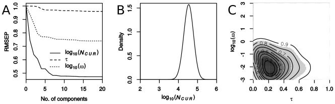
Figure 7: Root mean squared error of prediction (RMSEP) as a function of the number of components used for each parameter (A), marginal posterior estimate for parameter $log_{10}(N_{CUR})$ (B) and joint posterior for $\tau$ and $log_{10}(\omega)$ (C). Solid contour lines specify highest posterior density intervals.

The posterior estimates we obtained for parameters $N_{CUR}$, $\omega$ and $\tau$ (Figure 7 B and C) indicated a large population expansion that happened $\sim 13000$ generations ago to a present effective population size of $\sim 32000$. The credible intervals of the posterior estimates for $\omega$ and especially $\tau$ are large (Figure 7C) due to the small size of the downsampled data set. Additionally, the statistics used here seem not to be informative for parameter $\tau$ as indicated by the PLS analysis in Figure 7A. However, the more precise estimates for $N_{CUR}$ and $\omega$ are in good agreement with the findings of Boyko et al. (2008), who used a maximum likelihood method on the full data.

6 Appendix

Here we provide additional files required to replicate our population genetics example. First, we provide the input file popgen.par for fastsimcoal2 specifying the population genetics model used. Note that we decided to simulate the SFS using 10 independent loci with 1000 sites each.

fastsimcoal input file

⬇

//Number of population samples (demes)

1

//Population effective sizes (number of genes)

N_CUR

//Sample sizes

24

//Growth rates negative growth implies population expansion

0

//Number of migration matrices : 0 implies no migration between demes

0

//historical event: time, source, sink, migrants, new size, new growth rate,migr.matrix

1 historical events

T1 0 0 1 OMEGA 0 0

//Number of independent loci [chromosome]

10 0

//Per chromosome: Number of linkage blocks

1

//per Block: data type, num loci, rec. rate and mut rate

DNA 1000 0.00000 MUTRATE 0.33

Further, we provide the custom perl script calcPopstats.pl used to calculate summary statistics from site frequency spectra simulated with the program fastsimcoal2.

Perl script to calculate statistics from SFS

⬇

#!/usr/bin/perl -w

use strict;

#read fastsimcoal output SFS file

my $sfsfile=$ARGV[0];

open(FILE,"<",$sfsfile) or die "can’t open SFS file";

open (OUT, ">","summary_stats-temp.txt") or die "can’t open sum-stats file";

my ($firstline,$header,$sfsline)=(<FILE>,<FILE>,<FILE>);

#split sfsline into sfs

my @SFS=split /\t/,$sfsline;

my @stats;

#calculate stats

my ($sum,$S,$a1,$a2,$taj_D)=(0,0,0,0,0);

my $n=@SFS-2;

my ($b1,$b2)=(($n+1)/(3*($n-1)),2*($n**2+$n+3)/(9*$n*($n-1)));

#No. Segregating. sites S

for (my $i=1;$i<$n;$i++){

$sum=$sum+$i*($n-$i)*$SFS[$i];

$S=$S+$SFS[$i];

($a1,$a2)=($a1+1/$i,$a2+1/$i**2);

}

#Thita and pi

my ($thita,$pi)=($S/$a1,2*$sum/($n*($n-1)));

#Tajima’s D

my ($c1,$c2)=($b1-1/$a1,$b2-($n+2)/($a1*$n)+$a2/($a1**2));

my ($e1,$e2)=($c1/$a1,$c2/($a1**2+$a2));

if($S>0) {$taj_D=($pi-$S/$a1)/sqrt($e1*$S+$e2*$S*($S-1));}

#print out stats

@stats=($SFS[1],$S,$pi,$thita,$taj_D);

print OUT join("\t","sfs1","S","pi","thita","taj_D"),"\n",join("\t",@stats,"\n");

close(FILE);close(OUT);system("rm $sfsfile");

Finally, we provide the file PLSdef_popgen.txt specifying the PLS transformation of the 20 statistics (7 polymorphism statistics + their products) to 4 components. The first six columns in the file specify the boxcox transformation of the statistic and the remaining 4 columns specify the PLS components.

The file PLSdef_popgen.txt containing the definitions of the PLS transformations for ABCtoolbox

⬇

sfs1 1140 0 -17.58 1.06 0.06 0.07 0.22 0.27 -0.16 0.23

S 4478 0 -10.3 1.12 0.12 0.13 0.25 0.1 -0.3 0.11

pi 1730.18 0 -11.52 1.1 0.09 0.11 0.26 0.05 -0.27 0.07

thita 1199.16 0 -10.3 1.12 0.12 0.13 0.25 0.1 -0.3 0.11

taj_D 2.87 -2.19 0.61 1.48 0.51 0.19 0.11 -0.38 -0.53 -0.5

sfs1_X_sfs1 1299600 0 -20 1.02 0.01 0.02 0.21 0.29 0.13 -0.14

sfs1_X_S 5104920 0 -20 1.03 0.01 0.03 0.25 0.16 0.18 -0.12

sfs1_X_pi 1426520 0 -20 1.03 0.02 0.03 0.25 0.12 0.19 -0.11

sfs1_X_thita 1367040 0 -20 1.03 0.01 0.03 0.25 0.16 0.18 -0.12

sfs1_X_taj_D 634.38 -559.99 -0.61 1.48 0.66 0.09 0.15 -0.36 0.45 -0.01

S_X_S 20052500 0 -18.79 1.06 0.04 0.06 0.26 0.03 0.06 -0.08

S_X_pi 7455340 0 -20 1.06 0.03 0.05 0.26 -0.02 0.08 -0.07

S_X_thita 5369820 0 -18.79 1.06 0.04 0.06 0.26 0.03 0.06 -0.08

S_X_taj_D 8737.33 -1796.63 -9.09 1.21 0.61 0.06 0.18 -0.4 0.16 0.14

pi_X_pi 2993510 0 -20 1.05 0.02 0.04 0.26 -0.07 0.12 -0.05

pi_X_thita 1996450 0 -20 1.06 0.03 0.05 0.26 -0.02 0.08 -0.07

pi_X_taj_D 3508.27 -349.33 -13.94 1.14 0.35 0.05 0.18 -0.39 0.07 0.16

thita_X_thita 1437980 0 -18.79 1.06 0.04 0.06 0.26 0.03 0.06 -0.08

thita_X_taj_D 2339.76 -481.12 -9.09 1.21 0.61 0.06 0.18 -0.4 0.16 0.14

taj_D_X_taj_D 8.21 0 -6.67 1.12 0.13 0.12 0.06 -0.25 -0.3 0.78

References

- Adrion et al. [2014] Jeffrey R Adrion, Athanasios Kousathanas, Marta Pascual, Hannah J Burrack, Nick M Haddad, Alan O Bergland, Heather Machado, Timothy B Sackton, Todd a Schlenke, Masayoshi Watada, Daniel Wegmann, and Nadia D Singh. Drosophila suzukii: The Genetic Footprint of a Recent, Worldwide Invasion. Molecular biology and evolution, aug 2014. ISSN 1537-1719. doi: 10.1093/molbev/msu246. URL http://www.ncbi.nlm.nih.gov/pubmed/25158796.
- Aeschbacher et al. [2012a] Simon Aeschbacher, Mark a Beaumont, and Andreas Futschik. A Novel Approach for Choosing Summary Statistics in Approximate Bayesian Computation. Genetics, 192(November):1027–1047, September 2012a. ISSN 1943-2631. doi: 10.1534/genetics.112.143164.
- Aeschbacher et al. [2012b] Simon Aeschbacher, Mark A. Beaumont, and Andreas Futschik. A novel approach for choosing summary statistics in approximate bayesian computation. Genetics, 192(3):1027–1047, November 2012b. ISSN 0016-6731, 1943-2631. doi: 10.1534/genetics.112.143164.
- Barthelmé and Chopin [2011] Simon Barthelmé and Nicolas Chopin. ABC-EP: expectation propagation for likelihood-free Bayesian computation. In Proceedings of the 28th international conference on machine learning, Bellevue, WA., 2011.
- Beaumont et al. [2009] M. A. Beaumont, J.-M. Cornuet, J.-M. Marin, and C. P. Robert. Adaptive approximate Bayesian computation. Biometrika, 96(4):983–990, October 2009. ISSN 0006-3444. doi: 10.1093/biomet/asp052.
- Beaumont [2008] Mark A. Beaumont. Joint determination of topology, divergence time, and immigration in population trees. In S. Matsumura, P. Forster, and C. Renfrew, editors, Simulation, Genetics and Human Prehistory. McDonald Institute for Archaeological Research, United Kingdom, 2008.
- Beaumont et al. [2002] Mark A. Beaumont, Wenyang Zhang, and David J. Balding. Approximate Bayesian Computation in Population Genetics. Genetics, 162:2025–2035, December 2002.
- Blum and François [2010] M. G. B. Blum and O. François. Non-linear regression models for approximate bayesian computation. Statistics and Computing, 20(1):63–73, 2010. ISSN 0960-3174. doi: 10.1007/s11222-009-9116-0.
- Blum et al. [2013] M. G. B. Blum, M. A. Nunes, D. Prangle, and S. A. Sisson. A comparative review of dimension reduction methods in approximate bayesian computation. Statist. Sci., 28(2):189–208, 05 2013. doi: 10.1214/12-STS406.
- Boyko et al. [2008] Adam R Boyko, Scott H Williamson, Amit R Indap, Jeremiah D Degenhardt, Ryan D Hernandez, Kirk E Lohmueller, Mark D Adams, Steffen Schmidt, John J Sninsky, Shamil R Sunyaev, Thomas J White, Rasmus Nielsen, Andrew G Clark, and Carlos D Bustamante. Assessing the evolutionary impact of amino acid mutations in the human genome. PLoS Genetics, 4(5):e1000083, May 2008. ISSN 1553-7404. doi: 10.1371/journal.pgen.1000083.
- Bray et al. [2010] T. C. Bray, V. C. Sousa, B. Parreira, M. W. Bruford, and L. Chikhi. 2BAD: an application to estimate the parental contributions during two independent admixture events. Molecular Ecology Resources, 10(3):538–541, 2010.
- Chu et al. [2013] Jui-Hua Chu, Daniel Wegmann, Chia-Fen Yeh, Rong-Chien Lin, Xiao-Jun Yang, Fu-Min Lei, Cheng-Te Yao, Fa-Sheng Zou, and Shou-Hsien Li. Inferring the geographic mode of speciation by contrasting autosomal and sex-linked genetic diversity. Molecular biology and evolution, 30(11):2519–30, November 2013. ISSN 1537-1719. doi: 10.1093/molbev/mst140.
- Cornuet et al. [2008] Jean-Marie Cornuet, Filipe Santos, Mark A. Beaumont, Christian P. Robert, Jean-Michel Marin, David J. Balding, Thomas Guillemaud, and Arnaud Estoup. Inferring population history with DIY ABC: a user-friendly approach to approximate Bayesian computation. Bioinformatics, 24(23):2713–2719, 2008.
- Csilléry et al. [2012] Katalain Csilléry, Olivier François, and Michael G. B. Blum. abc: an R package for approximate Bayesian computation (ABC). Methods in Ecology and Evolution, 3:475–479, 2012.
- Cuesta-Albertos and Nieto-Reyes [2008] J. A. Cuesta-Albertos and A. Nieto-Reyes. The random tukey depth. Computational Statistics & Data Analysis, 52(11):4979–4988, July 2008. ISSN 0167-9473. doi: 10.1016/j.csda.2008.04.021.
- Didelot et al. [2011] Xavier Didelot, Richard G Everitt, Adam M Johansen, and Daniel J Lawson. Likelihood-free estimation of model evidence. Bayesian Analysis, 6(1):49–76, 2011. doi: 10.1214/11-BA602.
- Estoup et al. [2012] Arnaud Estoup, Eric Lombaert, Jean-Michel Marin, Thomas Guillemaud, Pierre Pudlo, Christian P Robert, and Jean-Marie Cornuet. Estimation of demo-genetic model probabilities with Approximate Bayesian Computation using linear discriminant analysis on summary statistics. Molecular ecology resources, 12(5):846–55, September 2012. ISSN 1755-0998. doi: 10.1111/j.1755-0998.2012.03153.x.
- Excoffier et al. [2013] Laurent Excoffier, Isabelle Dupanloup, Emilia Huerta-Sánchez, Vitor C. Sousa, and Matthieu Foll. Robust Demographic Inference from Genomic and SNP Data. PLoS Genetics, 9(10):e1003905, October 2013. ISSN 1553-7404. doi: 10.1371/journal.pgen.1003905.
- Fagundes et al. [2007] Nelson J. R. Fagundes, Nicolas Ray, Mark A. Beaumont, Samuel Neuenschwander, Francisco M. Salzano, Sandro L. Bonatto, and Laurent Excoffier. Statistical evaluation of alternative models of human evolution. Proceedings of the Natural Academy of Sciences U.S.A., 104(45):17614–17619, November 2007.
- Fearnhead and Prangle [2012] Paul Fearnhead and Dennis Prangle. Constructing summary statistics for approximate Bayesian computation: semi-automatic approximate Bayesian computation. Journal of the Royal Statistical Society: Series B (Statistical Methodology), 74(3):419–474, June 2012. ISSN 13697412. doi: 10.1111/j.1467-9868.2011.01010.x.
- Foll et al. [2008] Matthieu Foll, Mark A. Beaumont, and Oscar Gaggiotti. An approximate Bayesian computation approach to overcome biases that arise when using amplified fragment length polymorphism markers to study population structure. Genetics, 179:927–939, 2008.
- François and Guillaume [2011] Olivier François and Laval Guillaume. Deviance information criteria for model selection in approximate Bayesian computation. Statistical Applications in Genetics and Molecular Biology, 10(1):1–25, 2011.
- Gutenkunst et al. [2009] Ryan N Gutenkunst, Ryan D Hernandez, Scott H Williamson, and Carlos D Bustamante. Inferring the joint demographic history of multiple populations from multidimensional SNP frequency data. PLoS genetics, 5(10):e1000695, oct 2009. ISSN 1553-7404. doi: 10.1371/journal.pgen.1000695. URL http://www.pubmedcentral.nih.gov/articlerender.fcgi?artid=2760211{&}tool=pmcentrez{&}rendertype=abstract.
- Hickerson et al. [2007] Michael J. Hickerson, Eli Stahl, and Naoki Takebayashi. msBayes: Pipeline for testing comparative phylogeographic histories using hierarchical approximate Bayesian computation. BMC Bioinformatics, 8:268, July 2007. ISSN 1471-2105. doi: 10.1186/1471-2105-8-268. URL https://doi.org/10.1186/1471-2105-8-268.
- Jabot et al. [2013] Franck Jabot, Thierry Faure, and Nicolas Dumoulin. EasyABC: performing efficient approximate bayesian computation sampling schemes using r. Methods in Ecology and Evolution, 4(7):684–687, 2013. ISSN 2041-210X. doi: 10.1111/2041-210X.12050.
- Kousathanas et al. [2016] Athanasios Kousathanas, Christoph Leuenberger, Jonas Helfer, Mathieu Quinodoz, Matthieu Foll, and Daniel Wegmann. Likelihood-free inference in high-dimensional models. 203(2):893–904, 2016. ISSN 0016-6731, 1943-2631. doi: 10.1534/genetics.116.187567. URL http://www.genetics.org/content/203/2/893.
- Leuenberger and Wegmann [2010] Christoph Leuenberger and Daniel Wegmann. Bayesian computation and model selection without likelihoods. Genetics, 184(1):243–252, January 2010. ISSN 0016-6731, 1943-2631. doi: 10.1534/genetics.109.109058.
- Liepe et al. [2010] Juliane Liepe, Chris Barnes, Erika Cule, Kamil Erguler, Paul Kirk, Tina Toni, and Michael P. H. Stumpf. ABC-SysBio–approximate Bayesian computation in Python with GPU support. Bioinformatics, 26(14):1797–1799, 2010.
- Lopes et al. [2009] Joao S. Lopes, David Balding, and Mark A. Beaumont. PopABC: a program to infer historical demographic parameters. Bioinformatics, 25(20):2747–2749, 2009.
- Marjoram et al. [2003] Paul Marjoram, John Molitor, Vincent Plagnol, and Simon Tavaré. Markov chain monte carlo without likelihoods. Proceedings of the National Academy of Sciences, 100(26):15324–15328, December 2003. ISSN 0027-8424, 1091-6490. doi: 10.1073/pnas.0306899100.
- Pavlidis et al. [2010] Pavlos Pavlidis, Stefan Laurent, and Wolfgang Stephan. msABC: a modification of Hudson’s ms to facilitate multi-locus ABC analysis. Molecular Ecology Resources, 10(4):723–727, 2010.
- Peter et al. [2010] Benjamin M Peter, Daniel Wegmann, and Laurent Excoffier. Distinguishing between population bottleneck and population subdivision by a Bayesian model choice procedure. Molecular ecology, 19(21):4648–60, November 2010. ISSN 1365-294X. doi: 10.1111/j.1365-294X.2010.04783.x.
- Picchini [2014] Umberto Picchini. Inference for SDE Models via Approximate Bayesian Computation. Journal of Computational and Graphical Statistics, 23(4):1080–1100, October 2014. ISSN 1061-8600. doi: 10.1080/10618600.2013.866048. URL https://doi.org/10.1080/10618600.2013.866048.
- Prangle et al. [2014] Dennis Prangle, Michael GB Blum, G Popovic, and SA Sisson. Diagnostic Tools for Appoximate Bayesian Compuation using the Coverage Property. Australian and New Zealand Journal of Statistics, 56(4):309–329, 2014. doi: 10.1111/anzs.12087.
- Pritchard et al. [1999] Jonathan K. Pritchard, Mark T. Seielstad, Anna Perez-Lezaun, and Marcus W. Feldman. Population growth of human Y chromosome: a study of Y chromosome microsatellites. Molecular Biology and Evolution, 16(12):1791–1798, 1999.
- Robert et al. [2011] Christian P. Robert, Jean-Marie Cornuet, Jean-Michel Marin, and Natesh S. Pillai. Lack of confidence in approximate bayesian computation model choice. Proceedings of the National Academy of Sciences, 108(37):15112–15117, September 2011. ISSN 0027-8424, 1091-6490. doi: 10.1073/pnas.1102900108.
- Sisson et al. [2007] SA A Sisson, Y Fan, and Mark MM Tanaka. Sequential Monte Carlo without likelihoods. Proceedings of the National Academy of Sciences of the United States of America, 104(6):1760–5, February 2007. ISSN 0027-8424. doi: 10.1073/pnas.0607208104.
- Tallmon et al. [2008] David A. Tallmon, Ally Koyuk, Gordon Luikart, and Mark A. Beaumont. ONeSAMP: a program to estimate effective population size using approximate Bayesian computation. Molecular Ecology Resources, 8:299–301, 2008.
- Tavaré et al. [1997] Simon Tavaré, David J. Balding, R. C. Griffiths, and Peter Donnelly. Inferring coalescence times from DNA sequence data. Genetics, 145:505–518, February 1997.
- Tenenhaus et al. [1995] M. Tenenhaus, J.P. Gauchi, and C. Ménardo. Régression PLS et applications. Revue de statistique appliquée, 43(1):7–64, 1995.
- Thornton [2009] Kevin R. Thornton. Automating approximate Bayesian computation by local linear regression. BMC Genetics, 10:35, 2009.
- Wegmann et al. [2009] Daniel Wegmann, Christoph Leuenberger, and Laurent Excoffier. Efficient approximate bayesian computation coupled with markov chain monte carlo without likelihood. Genetics, 182(4):1207–1218, August 2009. ISSN 0016-6731, 1943-2631. doi: 10.1534/genetics.109.102509. 00118 PMID: 19506307.
- Wegmann et al. [2010] Daniel Wegmann, Christoph Leuenberger, Samuel Neuenschwander, and Laurent Excoffier. ABCtoolbox: a versatile toolkit for approximate bayesian computations. BMC Bioinformatics, 11(1):116, March 2010. ISSN 1471-2105. doi: 10.1186/1471-2105-11-116. 00095 PMID: 20202215.