Two and three electrons on a sphere: A generalized Thomson problem

Abstract

Generalizing the classical Thomson problem to the quantum regime provides an ideal model to explore the underlying physics regarding electron correlations. In this work, we systematically investigate the combined effects of the geometry of the substrate and the symmetry of the wave function on correlations of geometrically confined electrons. By the numerical configuration interaction method in combination with analytical theory, we construct symmetrized ground-state wave functions; analyze the energetics, correlations, and collective vibration modes of the electrons; and illustrate the routine for the strongly correlated, highly localized electron states with the expansion of the sphere. This work furthers our understanding about electron correlations on confined geometries and shows the promising potential of exploiting confinement geometry to control electron states.

I Introduction

Inquiry into the physics of geometrically confined electrons is a prominent research theme in modern physics and chemistry Reimann and Manninen (2002); Sabin and Brandas (2009); Koning and Vitelli (2016), and it can be traced back to the classical problem of determining the ground state of classical charged particles confined on the surface of a sphere, which is known as the Thomson problem Thomson (1904); Nelson (2002); Bowick et al. (2002a); Levin and Arenzon (2003); Bausch et al. (2003); De Luca et al. (2005); Wales and Ulker (2006); Wales et al. (2009); Mehta et al. (2016). The Thomson problem and its various generalized versions arise in diverse physical systems Dinsmore et al. (2002); Bowick et al. (2002a, 2006); Cioslowski (2009); Koning and Vitelli (2016); Agboola et al. (2015); Yao (2016, 2017); Chen et al. (2018), ranging from surface ordering of liquid-metal drops Davis (1997), colloidal particles Bausch et al. (2003), and protein subunits over spherical viruses Caspar and Klug (1962); Lidmar et al. (2003) to mechanical-instability-driven wrinkling crystallography on spherical surfaces Brojan et al. (2015). Recently, due to advances in semiconductor technology and spectroscopic probes, geometrically confined few-electron systems have been experimentally accessible, and they bring a host of scientific problems related to understanding electron correlations Kastner (1992); Ashoori (1996); Peeters and Schweigert (1996); Creffield et al. (1999); Cantele et al. (2001). Generalizing the classical Thomson problem to quantum regime provides an ideal model to explore the underlying physics regarding electron correlations. In comparison with the classical Thomson problem, its quantum version can exhibit richer physics beyond minimization of Coulomb potential energy. For example, even a single electron will interfere with itself when confined on the sphere. Furthermore, the Heisenberg uncertainty principle requires that the electrons are always restless even in the ground state.

Past studies have shown the crucial role of system size on electron states Ezra and Berry (1982); Ojha and Berry (1987); Watanabe and Lin (1987); Bao et al. (1997); Loos and Gill (2009a). On large spheres, the confined electrons become strongly correlated, which is closely related to Wigner crystallization of uniform electron gas Wigner (1934). Furthermore, studies of multiple-electron systems have revealed the fundamental role of symmetries of the wave function under rotation, inversion, and permutation and its non interaction feature on the nodal structure of electron states Bao et al. (1997); Loos and Bressanini (2015). Electron states of two- or three-electron systems on the sphere have been extensively studied using the approaches of approximate Schrödinger equations Ojha and Berry (1987); Loos and Gill (2009a); Seidl (2007) and the configuration interaction (CI) method Ezra and Berry (1982); Watanabe and Lin (1987); Loos and Gill (2009a); T. Helgaker (2013). Notably, the system of two electrons on a hypersphere has been quasiexactly solved, and the analytical results are useful in the development of correlation functionals within density-functional theory Loos and Gill (2009b, 2010, 2011). In this work, we focus on the combined effects of the geometry of the sphere and the symmetry of the wave functions on energetics and correlations of confined electrons. The model of the quantum version of the Thomson problem provides the opportunity to address fundamental questions with broader implications, such as the following: How do the electrons become correlated with the expansion of the sphere? What are the dynamic behaviors of the strongly correlated electrons?

To address these questions, we resort to the CI method in combination with analytical theory to construct and analyze the ground state wave functions of two- and three-electron systems Ezra and Berry (1982); Loos and Gill (2009a). Note that the CI method allows us to analyze the variation of the components composing the ground-state wave functions, and it provides insights into the enhancement of electron correlations. In this work, we construct symmetrized ground-state wave functions for both two- and three-electron systems. Energetics analysis shows the degeneracy of wave functions with distinct symmetries and the domination of the potential energy over the kinetic energy with the expansion of the sphere. In this process, eigenstates with larger angular momentum quantum numbers are excited under the increasingly important Coulomb interaction. Consequently, strongly correlated, highly localized electron states are established in the large-$R$ regime, as revealed in the probability analysis. In this regime, we propose a semi classical small-oscillation theory to quantitatively analyze the vibration modes and determine the symmetry-dependent quantum number of the ground-state harmonic oscillations. The results presented in this paper further our understanding about electron correlations in confined geometries and show the promising potential of exploiting confinement geometry to manipulate electron states.

II Model and Method

The ground-state wave function and energy of $N$ electrons on the sphere are determined by the time-independent Schrödinger equation:

$$\hat{H}\Psi(\{\vec{r}_{i}\})=E\Psi(\{\vec{r}_{i}\}),$$ (1)

where $\hat{H}=\hat{K}+\hat{V}$ and $\vec{r}_{i}$ is the position of electron $i$. The kinetic-energy term $\hat{K}=\sum_{i=1}^{N}\hat{L}_{i}^{2}/2R^{2}$, $R$ is the radius of the sphere, and $\hat{L}_{i}$ is the angular momentum operator of the electron $i$. The potential energy term $\hat{V}=\sum_{i<j}1/|\vec{r}_{i}-\vec{r}_{j}|$.

We resort to the CI method to construct the ground state wave functions with certain symmetries T. Helgaker (2013). The CI wave function consists of a linear combination of basis wave functions, whose expansion coefficients are variationally determined. This method can provide highly accurate wave functions, especially for systems with a small number of particles. The CI method has extensive applications in quantum chemistry due to the simple structure of the wave function Michael P. (2001). In practice, a truncated Hilbert space spanned by dominant eigenstates provides a good approximation for performing the diagonalization of the Hamiltonian.

We first construct the basis wave function $\Psi_{\mathbb{n}}(\{\vec{r}_{i}\})$, where $\mathbb{n}$ represents a complete set of quantum numbers to characterize the state of the system. For the two-electron system, $|\mathbf{n}\rangle=|l_{1},l_{2},l,m\rangle$, which is the common eigenstate of $\hat{L}^{2}$, $\hat{L}_{z}$, and $\hat{L}_{1}^{2}$. For the three-electron system, $|\mathbf{n}\rangle=|l_{12},l_{1},l_{2},l_{3},l,m\rangle$, which is the common eigenstate of the mutually commuting $\hat{L}_{12}^{2}$, $\hat{L}_{1}^{2}$, $\hat{L}_{2}^{2}$, $\hat{L}_{3}^{2}$, $\hat{L}^{2}$, and $\hat{L}_{z}$. From the linear combination of $\Psi_{\mathbb{n}}(\{\vec{r}_{i}\})$, we construct wave functions $\Psi^{X_{p}}_{\mathbb{n}}(\{\vec{r}_{i}\})$ with certain symmetries. The superscript $X_{p}$ indicates that the wave function is exchange-symmetric ($X=S$) or exchange-antisymmetric ($X=A$), and has even ($p=e$) or odd ($p=o$) parity. The relevant matrix elements of the kinetic and potential energies are: $K^{X_{p}}_{\mathbb{n}\mathbb{n^{\prime}}}=\langle\Psi^{X_{p}}_{\mathbb{n}}|\hat{K}|\Psi^{X_{p}}_{\mathbb{n^{\prime}}}\rangle$, and $V^{X_{p}}_{\mathbb{n}\mathbb{n^{\prime}}}=\langle\Psi^{X_{p}}_{\mathbb{n}}|\hat{V}|\Psi^{X_{p}}_{\mathbb{n^{\prime}}}\rangle$.

In this work, the units of length, energy and angular momentum are the Bohr radius $a_{B}=4\pi\epsilon_{0}\hbar^{2}/m_{e}e^{2}$, $e^{2}/4\pi\epsilon_{0}a_{B}$, and $\hbar$, respectively. $R/r_{B}\ll 1$ and $R/r_{B}\gg 1$ in the small- and large-$R$ regimes, respectively.

III Results and discussion

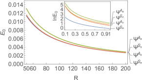
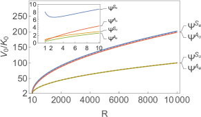
Figure 1: Energetics analysis of the two-electron ground states of distinct symmetries. In the notation $\Psi^{X_{p}}$ for the ground-state wave function, the superscript $X_{p}$ indicates that it is exchange symmetric ($X=S$) or exchange antisymmetric ($X=A$), and has even ($p=e$) or odd ($p=o$) parity. (a) Plot of the ground-state energy $E_{0}$ vs the radius $R$ of the sphere. Energy degeneracies are found in the large- and small-$R$ regimes. (b) The potential energy $V_{0}$ dominates over the kinetic energy $K_{0}$ in the large-$R$ regime. Solid lines are from the CI method. Dashed lines are from the small-oscillation theory.

III.1 The case of two electrons

For a two-electron system, the construction of the ground-state wave function must obey the Pauli exclusion principle. The orbital wave function of the two-electron system is either exchange-symmetric or exchange-antisymmetric depending on the spin state of the electrons. We discuss both cases in this section.

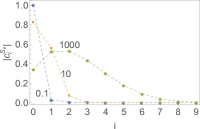
(a)  $\Psi^{S_{e}}$

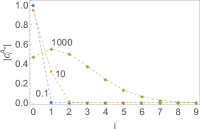
(b)  $\Psi^{A_{o}}$

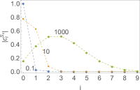
(c)  $\Psi^{S_{o}}$

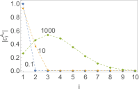
(d)  $\Psi^{A_{e}}$

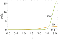
(e)  $\Psi^{S_{e}}$

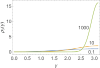
(f)  $\Psi^{A_{o}}$

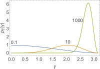
(g)  $\Psi^{S_{o}}$

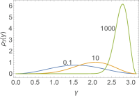
(h)  $\Psi^{A_{e}}$

Figure 2: Analysis of the ground state wave functions for the two-electron system constructed based on the CI method. The number near each curve indicates the value of $R$. (a)-(d) Plot of the amplitude of the angular momentum quantum number $i$ at varying $R$. (e)-(h) Distribution of the reduced probability density $\rho_{2}(\gamma)$, which is defined in Eq.(2). $\gamma$ is the angular distance of the two electrons.

Construction of symmetrized ground state wave functions For the two-electron system, the common eigenstates $|l_{1},l_{2},l,m\rangle$ of $\hat{L}^{2}$, $\hat{L}_{z}$, $\hat{L}_{1}^{2}$, $\hat{L}_{2}^{2}$ constitute the bases of the complete Hilbert space, denoted as $\mathscr{H}$. Note that $|l_{1},l_{2},l,m\rangle$ can be constructed by direct products of single particle states using Clebsch-Gordan coefficients L. D. Landau and E. M. Lifshitz (1981). From the basis wave function $\Psi_{\mathbb{n}}(\vec{r}_{1},\vec{r}_{2})$, where $\mathbb{n}=(l_{1},l_{2},l,m)$, one can construct wave functions $\Psi_{\mathbb{n}}^{X_{p}}(\vec{r}_{1},\vec{r}_{2})$ with a certain symmetry $X_{p}$.

To implement the CI method, we first notice that the Hilbert space $\mathscr{H}$ can be reduced to the sum of the subspaces $\mathscr{H}(l,m)$: $\mathscr{H}=~{}\mathop{\oplus}\limits_{l,m}\mathscr{H}(l,m)$. The subspace $\mathscr{H}(l,m)$ is spanned by the bases $\varepsilon(l,m)$: $\varepsilon(l,m)=\big{\{}|l_{1},l_{2},l,m\rangle\big{|}l_{1},l_{2}=0,1,2...\big{\}}$, where $|l_{1}-l_{2}|\leq l\leq l_{1}+l_{2}$ and $-l\leq m\leq l$. We search for the ground state wave functions in the subspaces of $\mathscr{H}(0,0)$ and $\mathscr{H}(1,0)$. According to angular momentum algebra, all the basis wave functions in $\mathscr{H}(0,0)$ are exchange-symmetric and with even parity Loos and Gill (2009a). That is, $\varepsilon(0,0)=\varepsilon^{S_{e}}(0,0)=\{|i,i,0,0\rangle\big{|}i=0,1,2...\}$. The bases of the subspace $\mathscr{H}(1,0)$ can be classified according to their parity and exchange symmetry: $\varepsilon(1,0)=\varepsilon^{S_{o}}(1,0)\oplus\varepsilon^{A_{e}}(1,0)\oplus\varepsilon^{A_{o}}(1,0)$. Specifically, $\varepsilon^{S_{o}}(1,0)=\{\frac{1}{\sqrt{2}}(|i,i+1,1,0\rangle+|i+1,i,1,0\rangle)\big{|}i=0,1,2...\}$, $\varepsilon^{A_{e}}(1,0)=\{|i,i,1,0\rangle\big{|}i=1,2...\}$, $\varepsilon^{A_{o}}(1,0)=\{\frac{1}{\sqrt{2}}(|i,i+1,1,0\rangle-|i+1,i,1,0\rangle)\big{|}i=0,1,2...\}$. Note that no base of the subspace $\mathscr{H}(1,0)$ is both exchange symmetric and with even parity. In fact, any wave function in $\mathscr{H}(1,0)$ with even parity must be exchange antisymmetric (see SI).

We denote the basis states in $\mathscr{H}^{S_{e}}(0,0)$, $\mathscr{H}^{S_{o}}(1,0)$, $\mathscr{H}^{A_{e}}(1,0)$ and $\mathscr{H}^{A_{o}}(1,0)$, as $|\Psi_{i}^{X_{p}}\rangle$, where $i$ completely determines the values of $l_{1},l_{2},l,m$ in $\varepsilon(l,m)$, as shown in preceding discussion. Any state in these subspaces can be expressed as a linear superposition of $|\Psi_{i}^{X_{p}}\rangle$: $|\Psi^{X_{p}}\rangle=\sum\limits_{i=i_{0}}^{i_{max}}c^{X_{p}}_{i}|\Psi^{X_{p}}_{i}\rangle$. In our numerical construction of the ground-state wave functions, $i_{0}=1$ for $|\Psi^{A_{e}}\rangle$, and $i_{0}=0$ for $|\Psi^{S_{e}}\rangle$, $|\Psi^{S_{o}}\rangle$, and $|\Psi^{A_{o}}\rangle$. Here, $i_{max}=100$. We obtain the values for the coefficients $\{c_{i}^{X_{p}}\}$ by expanding the Hamiltonian in the Hilbert space spanned by $|\Psi^{X_{p}}_{i}\rangle$ and solving for the equation $\sum\limits_{i^{\prime}}H^{X_{p}}_{ii^{\prime}}c^{X_{p}}_{i^{\prime}}=Ec^{X_{p}}_{i}$.

Analysis of ground states In Fig. 1(a), we show the monotonous decrease of the ground-state energy $E_{0}$ with the radius $R$ of the sphere for the four kinds of wave functions with distinct symmetries. Among these four cases, the $\Psi^{S_{e}}$ state, which is in the Hilbert subspace of $\mathscr{H}(0,0)$, has the lowest energy. Note that our numerically solved energy of the $\Psi^{S_{e}}$ state agrees well with the previously reported exact values Loos and Gill (2009a) (see SI for more information).

Figure 1(a) also shows the degeneracy of the $\Psi^{S_{o}}$ and $\Psi^{A_{o}}$ states in the small-$R$ regime; and the degeneracy of the $\Psi^{S_{e}}$ and $\Psi^{A_{o}}$ states in the large-$R$ regime. As $R\to\infty$, all the four energy curves in Fig. 1(a) tend to converge towards $1/(2R)$. This result is consistent with the following scaling argument. Since the kinetic energy is inversely proportional to $1/R^{2}$ and the potential energy is inversely proportional to $1/R$, the potential energy will dominate, and the total energy will scale with $R$ in the form of $1/R$ in the large-$R$ limit.

To show the relative contributions of the potential and kinetic energies to the total energy $E_{0}$, we plot the $V_{0}/K_{0}$ vs $R$ curve in Fig. 1(b). With the increase of $R$, the potential energy will dominate over the kinetic energy. We also see the merging of the $\Psi^{S_{e}}$ and $\Psi^{A_{o}}$ and $\Psi^{S_{o}}$ and $\Psi^{A_{e}}$ curves in the large-$R$ regime. The $V_{0}/K_{0}$ curves in the small-$R$ regime are shown in the inset. Since the $\Psi^{S_{e}}$ state is in the subspace $\mathscr{H}(0,0)$, whose zeroth-order wave function has zero kinetic energy, the $\Psi^{S_{e}}$ curve is obviously above all the other three states in the $\mathscr{H}(1,0)$ space.

We further show the contribution of each $|\Psi^{X_{p}}_{i}\rangle$ component in the constructed ground state $|\Psi^{X_{p}}\rangle$ by analyzing the coefficients $|c^{X_{p}}_{i}|$. In Figs. 2(a)-2(d), we present the values of $|c^{X_{p}}_{i}|$ for the first ten angular momentum quantum numbers $i$. The four kinds of wave functions exhibit uniform behavior with the increase of $R$. The value of the dominant $i$, which is zero at $R=0.1$, increases with $R$. Meanwhile, increasing $R$ widens the $|c^{X_{p}}_{i}|$ curves. The underlying physics is as follows: $|\Psi^{X_{p}}_{i}\rangle$-components of larger $i$ are excited under the increasingly important Coulomb interaction with the expansion of the sphere.

To characterize the correlation of the two electrons on the sphere, we compute the reduced two-electron probability density $\rho_{2}(\gamma)$ as a function of their angular distance $\gamma$ Ezra and Berry (1982):

$$\rho_{2}(\gamma)=\int\int P(\vec{r}_{1},\vec{r}_{2})\delta(\hat{\vec{r}}_{1}\cdot\hat{\vec{r}}_{2}-\cos{\gamma})dS_{1}dS_{2},$$ (2)

where $P(\vec{r}_{1},\vec{r}_{2})$ is the probability density of finding electron 1 and electron 2 simultaneously at $\vec{r}_{1}$ and $\vec{r}_{2}$ on the sphere. According to Born’s statistical interpretation of quantum mechanics, $P(\vec{r}_{1},\vec{r}_{2})=|\Psi^{X_{p}}(\vec{r}_{1},\vec{r}_{2})|^{2}$. Since $\int\int P(\vec{r}_{1},\vec{r}_{2})dS_{1}dS_{2}=1$, the normalization condition for $\rho_{2}(\gamma)$ is $\int_{0}^{\pi}\rho_{2}(\gamma)\sin{\gamma}d\gamma=1$.

In Figs. 2(e)-2(h), we plot the $\rho_{2}(\gamma)$ curves for all the four kinds of $\Psi^{X_{p}}(\vec{r}_{1},\vec{r}_{2})$. We see that when $R$ is small, the correlation between the two electrons is relatively weak. With the increase of $R$, sharp peaks on the $\rho_{2}(\gamma)$ curves are developed at $\gamma=\pi$ [see Figs. 2(e) and 2(f)] or near $\gamma=\pi$ [Figs. 2(g) and 2(h)], which indicates the enhanced electron-electron correlation. These two kinds of electron localization at and near diametric poles correspond to different vibration modes, as will be shown in the next section. A comparison of Figs. 2(a)-2(d) and 2(e)-2(h) shows that the localization of the electrons at the diametric poles accompanies the widening of the $|c^{X_{p}}_{i}|$ curves. In other words, a strongly correlated electron state results from a combination of multiple monochromatic states. The configuration of two highly localized diametric electrons found on a large sphere is consistent with the preceding energetics analysis, and it has connections to Wigner crystallization occurring in the two-dimensional electron gas in a uniform, neutralizing background when the electron density is less than a critical value Wigner (1934).

The correlation between the two electrons can also be characterized by the mean inverse separation $\tilde{d}_{12}^{-1}$, which is defined as $\tilde{d}_{12}^{-1}=\int\int\frac{R}{|\vec{r}_{1}-\vec{r}_{2}|}|\Psi(\vec{r}_{1},\vec{r}_{2})|^{2}dS_{1}dS_{2}$. It is recognized that $\tilde{d}_{12}^{-1}=V_{0}R$. For all four kinds of $\Psi^{X_{p}}(\vec{r}_{1},\vec{r}_{2})$, we numerically show that $\tilde{d}_{12}^{-1}$ decreases monotonously with $R$, and asymptotically to $1/2$ in the large-$R$ limit.

Asymptotic behaviors in the small- and large-$R$ regimes In this section, we perform perturbation analysis in the small-$R$ regime, and propose small oscillation theory (which is also called “strong-coupling perturbation theory” Seidl (2007)) in the large-$R$ regime to discuss the asymptotic behaviors of the two-electron system. The presented theoretical results can also be used to rationalize the energy curves in Fig. 1.

We first apply perturbation theory to analyze the ratio of the potential and kinetic energies $V_{0}/K_{0}$ for all four kinds of wave functions $\Psi^{X_{p}}(\vec{r}_{1},\vec{r}_{2})$ in the small-$R$ regime. The total angular momentum quantum number in the unperturbed state (Coulomb interaction is turned off) is denoted $i_{0}$. The ground-state energy and wave function can be written as

$$E_{0}=E_{0}^{(0)}+E_{0}^{(1)}+E_{0}^{(2)}+...$$ (3)

$$|\Psi^{X_{p}}\rangle=|\Psi^{X_{p}(0)}\rangle+|\Psi^{X_{p}(1)}\rangle+|\Psi^{X_{p}(2)}\rangle+...$$ (4)

where $E^{(0)}_{0}=K^{X_{p}}_{i_{0}i_{0}}$, and $E^{(1)}_{0}=V^{X_{p}}_{i_{0}i_{0}}$. $\Psi^{X_{p}(1)}(\vec{r}_{1},\vec{r}_{2})=\sum_{i>i_{0}}c^{(1)}_{i}\Psi^{X_{p}}_{i}(\vec{r}_{1},\vec{r}_{2})$, where $c^{(1)}_{i}=V^{X_{p}}_{i_{0}i}/[i_{0}(i_{0}+1)-i(i+1)]$.

Keeping up to the first-order term, we have

$$\frac{V_{0}}{K_{0}}=\frac{R^{2}V_{i_{0}i_{0}}^{X_{p}}}{i_{0}(i_{0}+1)+\sum\limits_{i>i_{0}}i(i+1)|c^{(1)}_{i}|^{2}}$$

Note that both $RV_{i_{0}i_{0}}^{X_{p}}$ and $c^{(1)}_{i}/R$ are independent of $R$. Here, $i_{0}=1$ for $\Psi^{A_{e}}(\vec{r}_{1},\vec{r}_{2})$, and $i_{0}=0$ for $\Psi^{S_{e}}(\vec{r}_{1},\vec{r}_{2})$. For $\Psi^{S_{e}}(\vec{r}_{1},\vec{r}_{2})$, $V_{0}/K_{0}\sim 1/R$. For $\Psi^{S_{o}}(\vec{r}_{1},\vec{r}_{2})$, $\Psi^{A_{e}}(\vec{r}_{1},\vec{r}_{2})$, and $\Psi^{A_{o}}(\vec{r}_{1},\vec{r}_{2})$, $V_{0}/K_{0}\sim R$. These scaling laws are consistent with the inset in Fig. 1(b).

On a large sphere, the localized electrons at diametric poles, as shown in Figs. 2(e)-2(h), are inevitably subject to small vibration due to Heisenberg’s uncertainty principle. The two-particle case has been analyzed in the quantum regime Ojha and Berry (1987). However, it is a challenge to generalize the quantum treatment to multiple-particle cases. Here, we perform a semi classical analysis of the small vibration of the electrons that can be readily extended to the three-electron case.

The classical Hamiltonian to describe the small vibration of two particles around the diametric equilibrium positions at $(\bar{\theta}_{1}=\pi/2,\bar{\phi}_{1}=0)$ and $(\bar{\theta}_{2}=\pi/2,\bar{\phi}_{2}=\pi)$ on the sphere is

$$H=\frac{1}{2}R^{2}\sum\limits_{i=1}^{2}(\delta\dot{\theta}_{i}^{2}+\delta\dot{\phi}_{i}^{2})+\sum\limits_{i,j=1}^{2}(\delta\theta_{i}\delta\theta_{j}D^{1}_{ij} + \delta\phi_{i}\delta\phi_{j}D^{2}_{ij})$$ (6)

$$+ \frac{1}{2R}.$$

where $D^{1}=\frac{1}{8R}\left(\begin{array}[]{cc}1&1\\ 1&1\\ \end{array}\right)$, $D^{2}=\frac{1}{8R}\left(\begin{array}[]{cc}1&-1\\ -1&1\\ \end{array}\right)$.

With the orthogonal transformation

$$\vartheta_{1} =\frac{1}{\sqrt{2}}(\delta\theta_{1}+\delta\theta_{2})\quad\vartheta_{2}=\frac{1}{\sqrt{2}}(\delta\phi_{2}-\delta\phi_{1})$$

$$\vartheta_{3} =\frac{1}{\sqrt{2}}(\delta\theta_{1}-\delta\theta_{2})\quad\vartheta_{4}=\frac{1}{\sqrt{2}}(\delta\phi_{2}+\delta\phi_{1}),$$

Eq.(6) becomes

$$H=\frac{1}{2}R^{2}\sum\limits_{r=1}^{4}\dot{\vartheta}_{r}^{2}+\frac{1}{2}\sum\limits_{r=1}^{2}\omega^{2}R^{2}\vartheta_{r}^{2}+\frac{1}{2R},$$ (7)

where $\omega=R^{-\frac{3}{2}}/2$. $\vartheta_{1}$ and $\vartheta_{2}$ describe the relative vibration of the two electrons. The vibrational energy [the second term in Eq.(7)] is proportional to $R^{-\frac{3}{2}}$. $\vartheta_{3}$ and $\vartheta_{4}$ describe the rotation of the whole system around the $y-$ and $z$-axes, respectively. The rotational energy is proportional to $L(L+1)/R^{2}$, where $L$ is the angular momentum. The energy contribution from the rotation of the whole system [i.e., the terms associated with $\vartheta_{3}$ and $\vartheta_{4}$ in the first sum term of Eq. (7) can be ignored in comparison with that from the vibration of the electrons. We focus on the relative vibration of the electrons in the following discussion.

Quantization of the reduced Hamiltonian in Eq. (7) leads to the expression for the energy level of the two-electron system in the large-$R$ regime L. D. Landau and E. M. Lifshitz (1981):

$$E_{\{n\}}=(n+1)\hbar\omega+\frac{1}{2R}.$$ (8)

From Eq.(8), by the virial theorem, we obtain the asymptotic expression for ${V_{0}}/{K_{0}}$ at large $R$: ${V_{0}}/{K_{0}}\sim R^{\frac{1}{2}}$. Our numerical results based on the CI method conform to this scaling law, as shown in Fig. 1(b).

The value of the quantum number $n$ in Eq. (8) can be obtained from the number of peaks in the $\rho_{2}(\gamma)$ curve in Figs. 2(e)-2(h). For the cases of $\Psi^{S_{e}}$ and $\Psi^{A_{o}}$ in Figs. 2(e) and 2(h) (see the curves for $R=1000$), the most probable positions of the electrons are at the diametric poles, which correspond to the state of $n=0$. In contrast, $n=1$ for the other two systems, as shown in Figs. 2(f) and 2(g) (see the curves for $R=1000$), where the most probable angular distance of the two electrons slightly deviates from $\pi$. Therefore, by their vibration modes, the four kinds of states $\Psi^{X_{p}}$ can be classified into two categories with $n=0$ and $n=1$. This conclusion derived from small-oscillation theory is consistent with the result of perturbative analysis of Schrödinger’s equation in the large-$R$ regime Ojha and Berry (1987). The classification of the states $\Psi^{X_{p}}$ by the vibration modes can account for the degeneracies between $\Psi^{S_{e}}$ and $\Psi^{A_{o}}$ and $\Psi^{S_{o}}$ and $\Psi^{A_{e}}$ in the large-$R$ regime, as shown in Fig. 1(a).

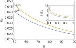
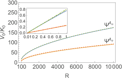
Figure 3: Energetics analysis of the three-electron ground states of distinct symmetries. (a) Plot of the ground-state energy $E_{0}$ vs the radius $R$ of the sphere. (b) The potential energy $V_{0}$ dominates over the kinetic energy $K_{0}$ in the large-$R$ regime. Solid lines are from the CI method. Dashed lines conform to a power law of exponent $3/2$, as derived from the small-oscillation theory. Dot-dashed lines (in inset) are linear functions of $R$ according to perturbation theory for small $R$.

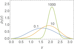
(a)  $\Psi^{A_{o}}$

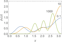
(b)  $\Psi^{A_{e}}$

Figure 4: Distribution of the reduced probability density $\rho_{3}(\gamma)$ in the three-electron system. $\rho_{3}(\gamma)$ is the probability of finding any two of the three electrons with angular separation $\gamma$.

III.2 The case of three electrons

For the three-electron system, we focus on the case of identical spin states. The ground-state wave functions must be exchange antisymmetric. We consider both odd and even parities. These ground-state wave functions are denoted as $\Psi^{A_{p}}$, where $p=e$ (even parity) or $p=o$ (odd parity). In comparison with the two-electron system, we find richer vibration modes for the three-electron system in the large-$R$ regime.

Construction of symmetrized ground-state wave functions For the three-electron system, $\hat{L}_{12}^{2}$, $\hat{L}_{1}^{2}$, $\hat{L}_{2}^{2}$, $\hat{L}_{3}^{2}$, $\hat{L}^{2}$, and $\hat{L}_{z}$ commute with each other. Their common eigenstate $|l_{12},l_{1},l_{2},l_{3},l,m\rangle$ is denoted as $|\mathbf{n}\rangle$. These eigenstates constitute the basis set $\varepsilon(l,m)$ of the Hilbert space $\mathscr{H}$. $\mathscr{H}=\mathop{\oplus}\limits_{l,m}\mathscr{H}(l,m)$. $\varepsilon(l,m)=\big{\{}|l_{12},l_{1},l_{2},l_{3},l,m\rangle\big{|}l_{1},l_{2},l_{3},l_{12}=0,1,2...\big{\}}$, where $|l_{1}-l_{2}|\leq l_{12}\leq l_{1}+l_{2},|l_{12}-l_{3}|\leq l\leq l_{12}+l_{3},-l\leq m\leq l$ (see SI). We construct the ground-state wave functions in the subspace $\mathscr{H}(0,0)$. $\varepsilon(0,0)=\{|l_{12}=l_{3},l_{1},l_{2},l_{3},l=0,m=0\rangle\}$, where the first equality is due to the zero total angular momenta. The basis set $\varepsilon(0,0)$ is completely determined by $\mathbb{L}=(l_{1},l_{2},l_{3})$.

By the standard coupling of three angular momentums, we obtain the eigenstate wave function of the three-electron system (see SI):

$$\Psi_{\mathbb{L}}(\vec{r}_{1},\vec{r}_{2},\vec{r}_{3}) =\sum\limits_{m_{1}=-l_{1}}^{l_{1}}\sum\limits_{m_{2}=-l_{2}}^{l_{2}}\left(\begin{array}[]{ccc}l_{1}&l_{2}&l_{3}\\ m_{1}&m_{2}&-m_{1}-m_{2}\end{array}\right)$$ (11)

$$\times\frac{1}{R^{3}}Y_{l_{1}}^{m_{1}}(\vec{n}_{1})Y_{l_{2}}^{m_{2}}(\vec{n}_{2})Y_{l_{3}}^{-m_{1}-m_{2}}(\vec{n}_{3}).$$ (12)

Note that by Eq. (11), $\Psi_{l_{1}l_{2}l_{3}}(\hat{P}_{ijk}\{\vec{r}_{1},\vec{r}_{2},\vec{r}_{3}\})=(-1)^{s(l_{1}+l_{2}+l_{3})}\Psi_{\hat{P}^{-1}_{ijk}\{l_{1}l_{2}l_{3}\}}(\vec{r}_{1},\vec{r}_{2},\vec{r}_{3})$. $\hat{P}_{ijk}$ is a permutation operator that changes the subscripts 1, 2, 3 of $r_{m}$ to $i$, $j$, $k$, respectively. $\hat{P}^{-1}_{ijk}$ changes the subscripts $i$, $j$, $k$ of $\ell_{m}$ to 1, 2, 3, respectively. $s=0$ and $1$ for even and odd permutations, respectively. This equation indicates that the new wave function is still in the basis set $\varepsilon(0,0)$ under the permutation of the three electrons. In the numerical construction of symmetrized ground state wave functions, we use 1360 allowed odd parity bases from $\Psi^{A_{o}}_{l_{1},l_{2},l_{3}}$ ($l_{1}\in[1,29]$, $l_{2},l_{3}\in[1,30]$) and 1120 allowed even parity bases from $\Psi^{A_{e}}_{1,2,3}$ ($l_{1}\in[1,27]$, $l_{2},\in[2,29]$, $l_{3}\in[3,30]$).

Analysis of ground states In Fig. 3(a), we show the monotonous decrease of the ground state energy $E_{0}$ with $R$ for both cases of $\Psi^{A_{o}}$ and $\Psi^{A_{e}}$. In the large-$R$ limit, both curves tend to converge towards $\sqrt{3}/R$, which is the potential energy of three classical electrons sitting on the vertices of a regular triangle circumscribed by the equator. In this asymptotic process up to $R=10000$, the ground-state energy of the $\Psi^{A_{o}}$ state is always slightly lower than that of the $\Psi^{A_{e}}$ state.

Figure 3(b) shows the ratio of the potential and kinetic energies for both kinds of wave functions. Similar to the case of the two-electron system, the potential energy will dominate over the kinetic energy with $R$, suggesting the Coulomb-potential-driven localization of electrons in the large-$R$ limit.

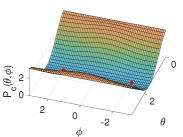
(a)  $\Psi^{A_{o}}$, $R=1$

(b)  $\Psi^{A_{o}}$, $R=10$

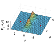
(c)  $\Psi^{A_{o}}$, $R=100$

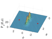
(d)  $\Psi^{A_{o}}$, $R=1000$

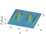
(e)  $\Psi^{A_{e}}$, $R=1$

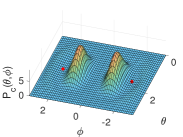
(f)  $\Psi^{A_{e}}$, $R=10$

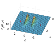
(g)  $\Psi^{A_{e}}$, $R=100$

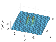
(h)  $\Psi^{A_{e}}$, $R=1000$

Figure 5: Probability density distribution $P_{c}(\theta,\phi)$ of any electron when the other two electrons are fixed at two vertices of a regular triangle circumscribed by the equator of the sphere. The fixed electrons are indicated by the red dots. The in-plane and out-of-plane vibrations of the electrons in the $\Psi^{A_{o}}$ and $\Psi^{A_{e}}$ states are characterized by $\{n_{1}=1,\ n_{2}=0\}$ and $\{n_{1}=0,\ n_{2}=3\}$, respectively. See text for more information.

In Fig. 4, we show the distribution of the probability density $\rho_{3}(\gamma)$ for both $\Psi^{A_{o}}(\vec{r}_{1},\vec{r}_{2},\vec{r}_{3})$ and $\Psi^{A_{e}}(\vec{r}_{1},\vec{r}_{2},\vec{r}_{3})$. $\rho_{3}(\gamma)$ is the probability of finding any two of the three electrons with angular separation $\gamma$. $\rho_{3}(\gamma)=8\pi^{2}R^{4}P(\vec{r}_{1},\vec{r}_{2})$, where $P(\vec{r}_{1},\vec{r}_{2})=\int P(\vec{r}_{1},\vec{r}_{2},\vec{r}_{3})dS_{3}$, and $P(\vec{r}_{1},\vec{r}_{2},\vec{r}_{3})=|\Psi^{A_{p}}(\vec{r}_{1},\vec{r}_{2},\vec{r}_{3})|^{2}$. The factor $8\pi^{2}$ arises from the normalization of $\rho_{3}(\gamma)$. From Fig. 4(a) for the case of $\Psi^{A_{o}}$, with the increase of $R$, we see the movement of the peak towards $\gamma=2.1\approx 2\pi/3$ and, simultaneously, the shrinking width of the peak. The value of $2\pi/3$ for $\gamma$ is recognized as the angular distance between any neighboring vertices in a triangular configuration of electrons on the equator. It signifies the enhanced correlation and localization of the electrons with $R$. In contrast, the $\Psi^{A_{e}}$ state exhibits distinct behaviors. From Fig. 4(b), we see three peaks on the curve of $R=1000$. These peaks correspond to distinct vibration modes, which will be discussed in the next section.

We also define the mean inverse separation $\tilde{d}_{ee}^{-1}$ of any two electrons to characterize their correlation. $\tilde{d}_{ee}^{-1}=\int\int\frac{R}{|\vec{r}_{i}-\vec{r}_{j}|}P(\vec{r}_{i},\vec{r}_{j})dS_{i}dS_{j}$. We recognize that $\tilde{d}_{ee}^{-1}=V_{0}R/3$. It is numerically shown that $\tilde{d}_{ee}^{-1}$ decreases monotonously with $R$ and approaches $1/\sqrt{3}\approx 0.577$ in the large-$R$ limit. Specifically, for $R$ increasing from 5000 to 10 000, $\tilde{d}_{ee}^{-1}$ decreases slightly from $0.582$ to $0.581$ for $\Psi^{A_{o}}$ and from $0.586$ to $0.584$ for $\Psi^{A_{e}}$.

Asymptotic behaviors in the small- and large-$R$ regimes In this section, we present asymptotic analysis of the ground states of the three-electron system in the small- and large-$R$ regimes. The relevant theoretical results are consistent with the energy curves in Fig. 3.

For small $R$, we perform perturbation analysis around the zeroth order wave function $\Psi^{A_{p}}_{\mathbf{L}_{0}}$, where the subscript refers to the state of $\mathbf{L}_{0}=\{l_{1}=1,l_{2}=1,l_{3}=1\}$ for $\Psi^{A_{o}}$ and $\mathbf{L}_{0}=\{l_{1}=1,l_{2}=2,l_{3}=3\}$ for $\Psi^{A_{e}}$. For both cases, $l=0$, and $m=0$. The zeroth- and first-order corrections to the ground-state energy $E_{0}$ are: $E^{(0)}_{0}=K_{0}=\left(l_{1}(l_{1}+1)+l_{2}(l_{2}+1)+l_{3}(l_{3}+1)\right)\hbar^{2}/R^{2}$, and $E^{(1)}_{0}=V^{A_{p}}_{\mathbf{L}_{0}\mathbf{L}_{0}}$. Specifically, $V^{A_{o}}_{\mathbf{L}_{0}\mathbf{L}_{0}}\approx 2.4/R$, $V^{A_{e}}_{\mathbf{L}_{0}\mathbf{L}_{0}}\approx 2.6/R$. Therefore, up to the first-order correction, we have $V_{0}/K_{0}=E^{(1)}_{0}/E^{(0)}_{0}\propto R$. This linear dependence of $V_{0}/K_{0}$ on $R$ agrees well with the numerical result presented in the inset of Fig. 3(b). For $R\leq 1$, the maximum deviation of $E_{0}$ from the CI method and the perturbation analysis up to the first-order correction is less than $1\%$ (see SI).

We proceed to analyze the small vibration of the three strongly correlated electrons in the large-$R$ regime. The equilibrium positions of the electrons are at the vertices of a regular triangle circumscribed by the equator of the sphere: $(\bar{\theta}_{1}=\pi/2,\bar{\phi}_{1}=0)$, $(\bar{\theta}_{2}=\pi/2,\bar{\phi}_{2}=2\pi/3)$, and $(\bar{\theta}_{3}=\pi/2,\bar{\phi}_{3}=4\pi/3)$. By introducing a set of collective coordinates $\eta_{r}$ ($r=1,2...6$) like in the treatment of the two-electron system, the classical Hamiltonian of the three-electron system is

$$H=\frac{1}{2}R^{2}\sum\limits_{r=1}^{6}\dot{\eta}_{r}^{2}+\frac{1}{2}\sum\limits_{r=1}^{3}\omega_{r}^{2}R^{2}\eta_{r}^{2}+\frac{\sqrt{3}}{R},$$ (13)

where $\omega_{1}=3^{-\frac{1}{4}}R^{-\frac{3}{2}}$, $\omega_{2}=\omega_{3}=(\sqrt{5}/2)\omega_{1}$ (see SI). These six collective coordinates describe three types of vibrations: the relative in-plane vibration between any two electrons (by $\eta_{1}$ and $\eta_{2}$), the out-of-plane vibration (by $\eta_{3}$), and the rotation of the whole system along three mutually perpendicular axes (by $\eta_{4}$, $\eta_{5}$, and $\eta_{6}$). In the large-$R$ regime, the vibrational energy is proportional to $R^{-3/2}$, and the rotational energy scales with $R$ in the form of $R^{-2}$ (see SI). By ignoring the rotational motion, quantization of the Hamiltonian in Eq. (13) leads to the following asymptotic expression for the energy levels in the three-electron system in the large-$R$ regime:

$$E_{\{n_{1},n_{2}\}}=(n_{1}+\frac{1}{2})\hbar\omega_{1}+(n_{2}+1)\hbar\omega_{2}+\frac{\sqrt{3}}{R}.$$ (14)

Applying the virial theorem to Eq. (14), we obtain the asymptotic expression for $V_{0}/K_{0}$: $\lim_{R\rightarrow\infty}V_{0}/K_{0}\rightarrow R^{\frac{1}{2}}$. The numerically solved $V_{0}/K_{0}$-$R$ curves as shown in Fig. 3(b) are in good agreement with this power law.

To characterize the correlation of the three electrons on the sphere, we calculate the probability density distribution $P_{c}(\theta,\phi)$ of any electron when the other two electrons are fixed at $\vec{r}^{\ast}_{2}=(\bar{\theta}_{2}=\frac{\pi}{2},\bar{\phi}_{2}=\frac{2\pi}{3})$ and $\vec{r}^{\ast}_{3}=(\bar{\theta}_{3}=\frac{\pi}{2},\bar{\phi}_{3}=-\frac{2\pi}{3})$. $P_{c}(\theta,\phi)=P(\vec{r},\vec{r}^{\ast}_{2},\vec{r}^{\ast}_{3})/P(\vec{r}^{\ast}_{2},\vec{r}^{\ast}_{3})$, where $P(\vec{r}^{\ast}_{2},\vec{r}^{\ast}_{3})=\int P(\vec{r}_{1},\vec{r}^{\ast}_{2},\vec{r}^{\ast}_{3})|dS_{1}$ and $P(\vec{r},\vec{r}^{\ast}_{2},\vec{r}^{\ast}_{3})=|\Psi^{A_{p}}(\vec{r},\vec{r}^{\ast}_{2},\vec{r}^{\ast}_{3})|^{2}$. A striking feature in the profiles of $P_{c}(\theta,\phi)$, as shown in Fig. 5, is the appearance of the double peaks. For the odd-parity case in Figs. 5(a)-5(d), the peaks near $\theta=0$ are out of the plane of the equator. In contrast, for the even-parity case shown in Figs. 5(e)-5(h), the peaks are in the plane of the equator. These two classes of ground-state vibration modes are completely determined by the parity of the wave function.

To determine the values for $n_{1}$ and $n_{2}$ in Eq.(14) in the ground states, we compare a series of $V_{0}/K_{0}$-$R$ curves using trial values for $n_{1}$ and $n_{2}$ with that from the CI method. It turns out that $n_{1}=1$, $n_{2}=0$ for $\Psi^{A_{o}}$, and $n_{1}=0$, $n_{2}=3$ for $\Psi^{A_{e}}$. The difference in the vibration modes is related to the distinct nodal structures caused by the opposite parities of $\Psi^{A_{o}}$ and $\Psi^{A_{e}}$ Bao et al. (1997). Here, it is of interest to note the appearance of the peaks in the $P_{c}(\theta,\phi)$ profiles even at relatively small $R$, as shown in Fig. 5(b) and 5(e). This observation suggests that the vibration modes are determined by the symmetry of the wave function instead of the size of the system. Increasing $R$ enhances these pre-existenting vibration modes.

IV Conclusion

In summary, we generalized the classical Thomson problem to the quantum regime to explore the underlying physics in electron correlations. We constructed symmetrized ground-state wave functions based on the CI method, systematically investigated the energetics and electron correlations, and proposed a small-oscillation theory to analyze the collective vibration modes of the electrons. As a key result of this work, we illustrated the routine to the strongly correlated, highly localized electron states with the expansion of the sphere. These results provide insights into the manipulation of electron states by exploiting confinement geometry. Finally, it is of interest to speculate on the connection of the $N$-electron system to the classical Thomson problem Bowick et al. (2002a, 2006). Despite the challenge in theory to construct the ground-state wave function of the $N$-electron system, experimentally, the spontaneous convergence of the electron state to the highly localized configuration with the expansion of the sphere may lead to a global solution to the 100-year-old, still unsolved classical Thomson problem Bowick et al. (2002a); Loos and Gill (2011); Agboola et al. (2015).

References

- Reimann and Manninen (2002) S. M. Reimann and M. Manninen, Rev. Mod. Phys. 74, 1283 (2002).
- Sabin and Brandas (2009) J. R. Sabin and E. J. Brandas, Theory of Confined Quantum Systems-Part One, Advances in Quantum Chemistry, Vol. 57 (Academic, 2009).
- Koning and Vitelli (2016) V. Koning and V. Vitelli, Crystals and Liquid Crystals Confined to Curved Geometries (Wiley, Hoboken, NJ, 2016).
- Thomson (1904) J. J. Thomson, Philos. Mag. 7, 237 (1904).
- Nelson (2002) D. R. Nelson, Defects and Geometry in Condensed Matter Physics (Cambridge University Press, Cambridge, 2002).
- Bowick et al. (2002a) M. Bowick, A. Cacciuto, D. R. Nelson, and A. Travesset, Phys. Rev. Lett. 89, 185502 (2002a).
- Levin and Arenzon (2003) Y. Levin and J. J. Arenzon, Europhys. Lett. 63, 415 (2003).
- Bausch et al. (2003) A. Bausch, M. Bowick, A. Cacciuto, A. Dinsmore, M. Hsu, D. Nelson, M. Nikolaides, A. Travesset, and D. Weitz, Science 299, 1716 (2003).
- De Luca et al. (2005) J. De Luca, S. B. Rodrigues, and Y. Levin, Europhys. Lett. 71, 84 (2005).
- Wales and Ulker (2006) D. J. Wales and S. Ulker, Phys. Rev. B 74, 212101 (2006).
- Wales et al. (2009) D. J. Wales, H. McKay, and E. L. Altschuler, Phys. Rev. B 79, 224115 (2009).
- Mehta et al. (2016) D. Mehta, J. Chen, D. Z. Chen, H. Kusumaatmaja, and D. J. Wales, Phys. Rev. Lett. 117, 028301 (2016).
- Dinsmore et al. (2002) A. Dinsmore, M. F. Hsu, M. Nikolaides, M. Marquez, A. Bausch, and D. Weitz, Science 298, 1006 (2002).
- Bowick et al. (2006) M. J. Bowick, A. Cacciuto, D. R. Nelson, and A. Travesset, Phys. Rev. B 73, 024115 (2006).
- Cioslowski (2009) J. Cioslowski, Phys. Rev. E 79, 046405 (2009).
- Agboola et al. (2015) D. Agboola, A. L. Knol, P. M. Gill, and P.-F. Loos, J. Chem. Phys. 143, 084114 (2015).
- Yao (2016) Z. Yao, Soft Matter 12, 7020 (2016).
- Yao (2017) Z. Yao, Soft Matter 13, 5905 (2017).
- Chen et al. (2018) J. Chen, X. Xing, and Z. Yao, Phys. Rev. E 97, 032605 (2018).
- Davis (1997) E. J. Davis, Aerosol Sci. Technol. 26, 212 (1997).
- Caspar and Klug (1962) D. L. Caspar and A. Klug, Cold Spring Harbor Symp. Quant. Biol. 27, 1 (1962).
- Lidmar et al. (2003) J. Lidmar, L. Mirny, and D. R. Nelson, Phys. Rev. E 68, 051910 (2003).
- Brojan et al. (2015) M. Brojan, D. Terwagne, R. Lagrange, and P. M. Reis, Proc. Natl. Acad. Sci. U.S.A. 112, 14 (2015).
- Kastner (1992) M. A. Kastner, Rev. Mod. Phys. 64, 849 (1992).
- Ashoori (1996) R. C. Ashoori, Nature (Landon) 379, 413 EP (1996).
- Peeters and Schweigert (1996) F. M. Peeters and V. A. Schweigert, Phys. Rev. B 53, 1468 (1996).
- Creffield et al. (1999) C. E. Creffield, W. Häusler, J. H. Jefferson, and S. Sarkar, Phys. Rev. B 59, 10719 (1999).
- Cantele et al. (2001) G. Cantele, D. Ninno, and G. Iadonisi, Phys. Rev. B 64, 125325 (2001).
- Ezra and Berry (1982) G. S. Ezra and R. S. Berry, Phys. Rev. A 25, 1513 (1982).
- Ojha and Berry (1987) P. C. Ojha and R. S. Berry, Phys. Rev. A 36, 1575 (1987).
- Watanabe and Lin (1987) S. Watanabe and C. D. Lin, Phys. Rev. A 36, 511 (1987).
- Bao et al. (1997) C. G. Bao, X. Yang, and C. D. Lin, Phys. Rev. A 55, 4168 (1997).
- Loos and Gill (2009a) P.-F. Loos and P. M. W. Gill, Phys. Rev. A 79, 062517 (2009a).
- Wigner (1934) E. Wigner, Phys. Rev. 46, 1002 (1934).
- Loos and Bressanini (2015) P.-F. Loos and D. Bressanini, J. Chem. Phys. 142, 214112 (2015).
- Seidl (2007) M. Seidl, Phys. Rev. A 75, 062506 (2007).
- T. Helgaker (2013) T. Helgaker, P. Jorgensen and J. Olsen, Molecular Electronic-Structure Theory (Wiley, Hoboken, NJ, 2013).
- Loos and Gill (2009b) P.-F. Loos and P. M. Gill, Phys. Rev. Lett. 103, 123008 (2009b).
- Loos and Gill (2010) P.-F. Loos and P. M. Gill, Mol. Phys. 108, 2527 (2010).
- Loos and Gill (2011) P.-F. Loos and P. M. Gill, J. Chem. Phys. 135, 214111 (2011).
- Michael P. (2001) M. M. Mueller., Fundamentals of Quantum Chemistry: Molecular Spectroscopy and Modern Electronic Structure Computations (Springer, 2001).
- L. D. Landau and E. M. Lifshitz (1981) L. D. Landau and E. M. Lifshitz, Quantum Mechanics, 3rd ed. (Butterworth-Heinemann, 1981).