Tunnelling-induced restoration of classical degeneracy in quantum kagome ice

Abstract

Quantum effect is expected to dictate the behaviour of physical systems at low temperature. For quantum magnets with geometrical frustration, quantum fluctuation usually lifts the macroscopic classical degeneracy, and exotic quantum states emerge. However, how different types of quantum processes entangle wave functions in a constrained Hilbert space is not well understood. Here, we study the topological entanglement entropy (TEE) and the thermal entropy of a quantum ice model on a geometrically frustrated kagome lattice. We find that the system does not show a $Z_{2}$ topological order down to extremely low temperature, yet continues to behave like a classical kagome ice with finite residual entropy. Our theoretical analysis indicates an intricate competition of off-diagonal and diagonal quantum processes leading to the quasi-degeneracy of states and effectively, the classical degeneracy is restored.

In systems with macroscopic ground state degeneracy, quantum correlation introduces non-trivial constraints on the Hilbert space, leading to the emergence of highly entangled quantum states of matter. The scenario is the gist in the studies of quantum Hall effect Prange and Girvin (1990.), flat band physics Tang et al. (2011); Neupert et al. (2011); Sun et al. (2011) and quantum spin liquids Anderson (1973, 1987); Moessner and Sondhi (2001a); Gingras and McClarty (2014); Zhou et al. (2017); Savary and Balents (2017a); Knolle and Moessner (2018). Among them, quantum magnets with geometrical frustration have become a fruitful playground to search for exotic quantum phases. In particular, spin ice systems on the corner-sharing tetrahedron lattices have attracted enormous attention due to their relevance to rare-earth pyrochlore materials Gingras and McClarty (2014); Gardner et al. (2010); Savary and Balents (2017a); Knolle and Moessner (2018) and the possibility to explore exotic quantum states of matter with anisotropic quantum exchange Hermele et al. (2004); Savary and Balents (2012); Lee et al. (2012); Shannon et al. (2012); Huang et al. (2014); Kato and Onoda (2015); Li et al. (2016); Li and Chen (2017); Savary and Balents (2017b).

Strong spin-orbit couplings in these materials lead to relatively unexplored anisotropic quantum effects. Dominant ferromagnetic Ising coupling in pyrochlore spin ice materials aligns spins along the local $\langle 111\rangle$ directions on the tetrahedron, and the system becomes geometrically frustrated at low temperatures. The macroscopically degenerate ground states obey the so-called “ice rules”, with two spins pointing in and two spins pointing out of the centre of each tetrahedron. By introducing different quantum tunnelling processes, it is possible to drive spin ice systems into various exotic quantum phases Hermele et al. (2004); Savary and Balents (2012); Shannon et al. (2012); Lee et al. (2012); Savary and Balents (2017b).

In addition to the intriguing physics in three dimensions, these pyrochlore spin ice materials also serve as a playground for studying quantum ice physics on a kagome lattice. The pyrochlore lattice can be visualized as alternating layers of triangular and kagome lattice stacking along the [111] direction (Fig. 1a). When an external field along this axis pins the spins on the triangular layer, effectively the system becomes decoupled layers of two-dimensional (2D) kagome lattices, provided the field is not too strong. This dimensional reduction partially reduces the degeneracy, and the ice rule is modified to the kagome ice rule with two spins pointing into each triangle, and one out (2-up-1-down in terms of the pseudo-spin), or vice versa, as shown in Fig. 1b.

Recently, numerical simulation on the kagome lattice that focuses on the pair-flipping process finds a gapped disordered quantum state, dubbed as quantum kagome ice (QKI)  Carrasquilla et al. (2015), which is argued to be an exotic $Z_{2}$ QSL. However, direct evidence characterising the non-trivial entanglement pattern in the ground state, such as the TEE, has not been analysed. Furthermore, how pair flipping processes induce quantum effects to the ice manifold is not clear. Using large-scale quantum Monte Carlo (QMC) simulations and degenerate perturbation theory (DPT), we show that the QKI state does not show a $Z_{2}$ topological order, but continues to behave like a classical kagome ice (CKI) due to the competition among different quantum tunnelling processes. Such competition originating from anisotropic exchange coupling could be relevant for pyrochlore material and recently synthesized tripod Kagome material Scheie et al. (2018).

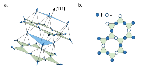
Figure 1: Geometry of pyrochlore lattice and the kagome layer. a. A pyrochlore spin ice consists of corner sharing tetrahedra of spins pointing into or out of each tetrahedron. The ferromagnetic coupling between nearest-neighbour spins leads to geometrical frustration, where spins on each tetrahedron follow a ’2-in-2-out’ ice rule. Pinning the spin on the triangular layers by applying a strong enough field along the [111] direction reduces the pyrochlore lattice to decoupled kagome layers (green layers). b. Kagome lattice can be viewed as corner-sharing triangles, or equivalently, corner-sharing hexagons. In a field, pseudo-spins on each triangle satisfies the kagome ice rule with ’2-up-1-down’ or ’2-down-1-up’ depending on the sign of the field ( $h>0$ here).

I Results

Quantum kagome ice model with pair-flipping interaction— On a kagome lattice, the nearest-neighbour, symmetry-allowed exchange interactions for the ground state dipolar-octupolar doublets can be modelled with an effective pseudo-spin-1/2 XYZh model Carrasquilla et al. (2015),

$$H_{\textrm{XYZh}}=\sum_{\langle\mathbf{r},\mathbf{r}^{\prime}\rangle}J_{z}S^{z}_{\mathbf{r}}S^{z}_{\mathbf{r}^{\prime}}-h\sum_{\mathbf{r}}S^{z}_{\mathbf{r}}-\sum_{\langle\mathbf{r},\mathbf{r}^{\prime}\rangle}\frac{J_{\pm}}{2}\left(S^{+}_{\mathbf{r}}S^{-}_{\mathbf{r}^{\prime}}+S^{-}_{\mathbf{r}}S^{+}_{\mathbf{r}^{\prime}}\right)+\frac{J_{\pm\pm}}{2}\left(S^{+}_{\mathbf{r}}S^{+}_{\mathbf{r}^{\prime}}+S^{-}_{\mathbf{r}}S^{-}_{\mathbf{r}^{\prime}}\right)$$ (1)

where $J_{z}>0$, $\mathbf{r}$ labels kagome lattice sites, and $\langle\mathbf{r},\mathbf{r}^{\prime}\rangle$ denotes the nearest-neighbour pairs. The first two terms correspond to the CKI model in a field, the third term corresponds to the hopping exchange and the last term is the pair-flipping interaction. We emphasize that even though the model is derived from the dipolar-octupolar doublets, the anisotropic exchange is ubiquitous in related materials, and we focus on the simplest anisotropic exchange term, $S^{+}_{\bm{r}}S^{+}_{\bm{r}^{\prime}}$, in the system that can be simulated with large-scale QMC. In the following, we set $J_{z}=1$ unless explicitly stated otherwise.

For $J_{\pm\pm}=0$ and $J_{\pm}>0$, this model is equivalent to the XXZ model with an external field. Previous studies show the ground state as a valence-bond solid (VBS) phase with a three-fold degeneracy Isakov et al. (2006); Damle and Senthil (2006). With $J_{\pm}=0$ and $J_{\pm\pm}<0$, recently the model is proposed to harbour a $Z_{2}$ QSL both numerically Carrasquilla et al. (2015) and theoretically Huang and Hermele (2017). Note that the parameter space of $J_{\pm\pm}>0$ and $J_{\pm\pm}<0$ are physically equivalent, connected via a unitary transformation $S^{+}\to iS^{+}$. Without loss of generality, here, we analyse model (1) with $J_{\pm\pm}<0$.

Topological entanglement entropy— For a quantum system with short-range interaction, the Renyi entanglement entropy between subregion $A$ and its complement obeys the so-called area law,

$$S_{n}(A)=\kappa l-\eta\gamma+O(L^{-1}),$$ (2)

where $\kappa$ is a non-universal constant and $l$ is the boundary length of the subregion. $\gamma$ is the TEE and $\eta$ is related to the number of (disconnected) boundaries. As a universal constant, the TEE plays the role of “order parameter” for detecting the hidden topological order in the system Kitaev and Preskill (2006); Levin and Wen (2006). The value of the TEE is related to the quantum dimension $\mathcal{D}$ with $\gamma=\ln\mathcal{D}$ that characterises the quasi-particle fractionalization of the topological order Kitaev and Preskill (2006). For a system with $Z_{2}$ topological order, the quantum dimension $\mathcal{D}=2$, and $\gamma=\ln 2$ is expected  Rowell et al. (2009); Jiang et al. (2012).

We measure the quantum entanglement using the second Renyi entropy Isakov et al. (2011); Cirac et al. (2011),

$$S_{2}(A)=-\ln\textrm{Tr}({\rho_{A}^{2}}),$$ (3)

where $\rho_{A}$ is the reduced density matrix of subregion $A$. Using the replica trick Isakov et al. (2011), we measure $S_{2}$ with four different subregions (Fig. 2a) that are strategically designed to eliminate the area terms Levin and Wen (2006), and

$$2\gamma=-S_{2}(R_{1})-S_{2}(R_{2})+S_{2}(R_{3})+S_{2}(R_{4}).$$ (4)

Fig. 2a shows TEE as a function of the inverse temperature $\beta=1/T$ with parameters in the QKI regime ($J_{\pm\pm}=-0.49$, $J_{\pm}=0$, and $h=0.833$). We find $\gamma$ is far below the expected $\ln 2$ value even at a temperature as low as $T\approx 1/48(\beta=48)$, indicating the system does not have a $Z_{2}$ topological order. The small finite $\gamma$ at low temperature is due to sub-leading corrections that cannot be cancelled. This result suggests two possibilities: either the QKI state is a short-range entangled symmetry protected topological order or the quantum fluctuations couple different kagome ice states in such a manner that the system behaves classically. We clarify this issue through the study of thermal entropy at low temperature.

Thermal entropy— The ground states of the XYZh model (1) in the classical limit satisfy the 2-up-1-down kagome ice rule and are extensively degenerate, leading to a residual entropy per spin $S/N=0.108$ Moessner and Sondhi (2001b).

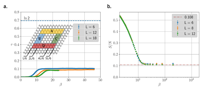
Figure 2: Topological entanglement entropy and thermal entropy. a. Topological entanglement entropy (TEE) as a function of the inverse temperature $\beta=1/T$ with parameters in the QKI phase ($J_{\pm\pm}=-0.49$ , $J_{\pm}=0$, and $h=0.833$). The system size is $N$=3$\times L\times L$. $\gamma$ converges to a value far smaller than $\ln 2$ (blue horizontal line), indicating the system does not show a $Z_{2}$ topological order. Four regions in Eq. (4) are defined as $R_{1}\equiv A\cup B\cup D$, $R_{2}\equiv A\cup C\cup D$, $R_{3}\equiv A\cup D$ and $R_{4}\equiv A\cup B\cup C\cup D$. b. Thermal entropy per spin $S/N$ as a function of $\beta$ in the QKI phase ( $J_{\pm\pm}=-0.45$ , $J_{\pm}=0$ , $h=1$). The low temperature plateau is consistent with the residual entropy per spin of a CKI (brown horizontal dot-dashed line).

In order to directly measure the thermal entropy in our QMC simulations, we employ the Wang-Landau method Troyer et al. (2004). We observe the thermal entropy remains finite at an extremely low temperature $T=1/200(\beta=200)$ with the value corresponding to the residual entropy per spin of a CKI. This classical behaviour in the supposedly quantum region is counter-intuitive. The system neither enters an ordered phase through the quantum order-by-disorder scheme Villain et al. (1980); Savary et al. (2012); Zhitomirsky et al. (2012) nor becomes a highly entangled disordered quantum state. To solve this puzzle, we analyse possible quantum processes out of the CKI manifold using DPT Bergman et al. (2007a, b).

Degenerate Perturbation Theory— Starting from the classical model, we treat all the quantum fluctuations as perturbations. It is useful in the following analysis to view the kagome lattice as corner-sharing hexagons; thus, all the non-trivial perturbation processes are within a single star of David (Fig. 3a). Due to the presence of the field that splits the degeneracy of the kagome ice rule on each triangle, the 2-up-1-down configurations are favoured. Spin configuration on each star is therefore uniquely determined by the hexagon configuration (Fig. 3b) that determines the process in the perturbation theory.

First, we consider the case $J_{\pm\pm}\neq 0$ and $J_{\pm}=0$ where the proposed QKI is realized. The leading non-trivial processes appear at the sixth-order of perturbation, and an effective Hamiltonian $\hat{P}_{6}$ can be written as,

$$\hat{P}_{6} =H_{d}+K_{pp}\sum_{\forall\hexagon n=3}H_{\hexagon,n=3}$$ (5)

$$H_{d} =D_{4,a}\sum_{\forall\hexagon n=4,a}H_{\hexagon,n=4,a}+D_{4,b}\sum_{\forall\hexagon n=4,b}H_{\hexagon,n=4,b}$$

$$+D_{5}\sum_{\forall\hexagon n=5}H_{\hexagon,n=5}$$

$$+D_{6}\sum_{\forall\hexagon n=6}H_{\hexagon,n=6}.$$ (6)

$H_{\hexagon,n=3}$ acts on an $n$=3 hexagon to generate an effective ring-exchange process, as shown in Fig. 3c, which brings one CKI configuration to a different one. In addition to the ring-exchange term, various non-trivial diagonal terms $H_{d}$ appear at the same order of perturbation acting on hexagons $n\geq 4$. For the case of $n=4$, there exist two different terms $H_{\hexagon,n=4,a}$ and $H_{\hexagon,n=4,b}$ acting on the $a$ and $b$ types of hexagons (Fig. 3b) respectively. The coefficients of these processes can be directly computed in DPT (See Supplementary Information for details). In the case of $h=J_{z}$, we have $K_{pp}=-\frac{58}{81}\Gamma$, $D_{4,b}=-\frac{1}{6}\Gamma$, $D_{4,a}=-\frac{1}{36}\Gamma$, $D_{5}=-\frac{289}{5292}\Gamma$, $D_{6}=-\frac{2}{49}\Gamma$, where $\Gamma={J_{\pm\pm}^{6}}/{J_{z}^{5}}$.

Consider the other limiting case where $J_{\pm}\neq 0$ and $J_{\pm\pm}=0$. The lowest non-trivial process occurs at the third order of perturbation, with an effective Hamiltonian,

$$\hat{P}_{3}=K_{np}\sum_{\forall\hexagon n=3}H_{\hexagon,n=3}+c,$$ (7)

where $K_{np}=-12{J^{3}_{\pm}}/{J_{z}^{2}}$. All diagonal processes at this level contribute to an overall constant energy shift $c$ which is irrelevant. The ring-exchange term $H_{\hexagon,n=3}$ drives the system into a VBS ground state Isakov et al. (2006); Damle and Senthil (2006).

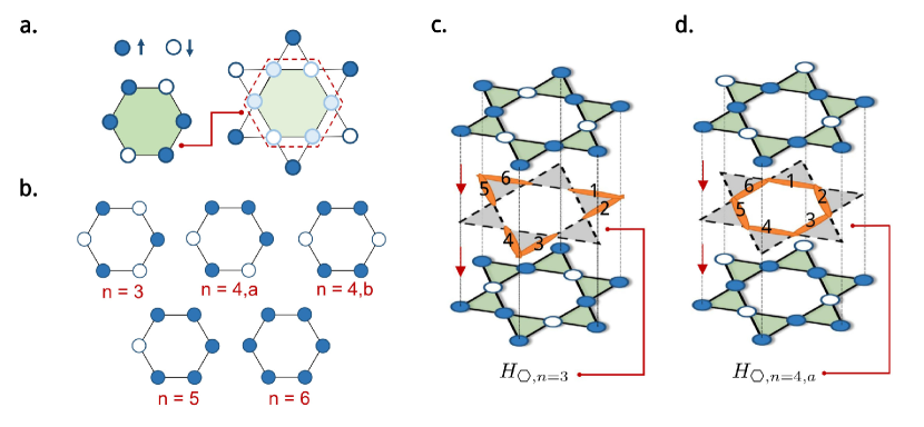
Figure 3: Hexagon units and quantum tunnelling processes. a. In a field, spins on each triangle follow the 2-up-1-down rule. When the spin configuration on the hexagon is determined, the configuration of the remaining spins within the star of David is uniquely defined. b. The allowed hexagon configurations in a field, classified according to the number of up-spins $n$. c. Example of the off-diagonal tunnelling term $H_{\hexagon,n=3}$ formed by six nearest-neighbour $S^{\pm}S^{\pm}$ operators on the orange bonds that couples two different $n=3$ CKI states . (d) Example of the diagonal tunnelling term $H_{\hexagon,n=4,a}$ that couples the same $n=4,a$ CKI states.

Fig. 4a shows a schematic picture to illustrate the effects coming from the diagonal and off-diagonal quantum tunnelling processes. For a QKI ($J_{\pm\pm}\neq 0$ and $J_{\pm}=0$), the introduction of the off-diagonal ring-exchange $H_{\hexagon,n=3}$ selects the three-fold degenerate VBS state out of the degenerate classical ice manifold, leaving all other states at higher energies. Adding the diagonal terms, reconfiguration of the energy levels occurs. These terms tend to maximize the overall fraction of $n$=4, 5, 6 hexagons while minimizing the fraction of $n$=3 hexagons. The competition between diagonal and off-diagonal processes reorganizes the states into quasi-degenerate levels and the classical degeneracy is restored. On the other hand, for the case $J_{\pm}\neq 0$ and $J_{\pm\pm}=0$, the process terminates at the ring-exchange level, and the VBS ground state is selected.

We further demonstrate this mechanism by measuring $P_{n}$, the fraction of hexagons with $n$ up spins using QMC (Fig. 4b). For the VBS parameters, the weight of $n$=3 hexagons $P_{3}$ dramatically increases at low temperature, accompanied with the decrease of $P_{4}$ . On the other hand, for the QKI parameters, the fractions for each type of hexagons remain unchanged, suggesting the system remains within the CKI state down to temperature much lower than the perturbative energy scale. Although DPT is expected to work only in the small $J_{\pm\pm}/J_{z}$ limit, the QMC results indicate the competition between these quantum tunnelling processes is indeed nonperturbative.

To illustrate the quantum origin of this quasi-degeneracy, we study the effective model using exact diagonalisation. Here, we slightly modify the effective Hamiltonian by introducing a tuning parameter $\alpha$ in order to change the weight of the diagonal process,

$$\hat{P}_{6}(\alpha)=\alpha H_{d}+K_{pp}\sum_{\forall\hexagon n=3}H_{\hexagon,n=3}.$$ (8)

Since the exact weight ratio between the two types of processes in the original XYZh model is unknown, tuning $\alpha$ provides information for how the energy spectrum is affected by adding the diagonal term.

For $\alpha=0$ where the ring-exchange dominates, the ground state should be the three-fold degenerate VBS state. Due to the finite size effect, the three lowest energy states in our ED results are not exactly degenerate. However, a detailed analysis of the wave function confirms these states correspond to the VBS state and becomes degenerate in the thermodynamic limit (See Supplementary Information). For $\alpha\to\infty$, the model corresponds to keeping only the diagonal terms. Therefore, all the classical kagome ice configurations are eigenstates of the Hamiltonian. We find the ground states are also three-fold degenerate, and corresponds to the three charge-ordered states in the classical kagome ice Chern et al. (2011); Wolf and Schotte (1988).

We expect there should be a level crossing at some intermediate $\alpha$, which indeed occurs somewhere around $\alpha=1.703\sim 1.778$ (Fig. 5a). Also, we find that the spectrum is compressed toward the ground state. To give a quantitative measure of this compression, we set an energy cutoff $\epsilon/N_{p}=0.00082$ and study how the number of levels below this cutoff, $N_{lv}$, changes with $\alpha$. We observe that the $N_{lv}$ increases as $\alpha$ increases, indicating a compression of energy levels toward the ground states, until after $\alpha>1.703$ (Fig. 5b). This suggests the quasi-degeneracy observed in our QMC simulation is a consequence of the compressed spectrum due to the competition between diagonal and off-diagonal term. With this physical picture in mind, we expect by tuning $K_{pp}$ in the effective Hamiltonian (6), the VBS phase should emerge with large enough $K_{pp}$. This can be realized in the original XYZh model by including both nonzero $J_{\pm}$ and $J_{\pm\pm}$ terms. The emergence of VBS by adding a small $J_{\pm}$ in QKI is then confirmed from the peaks of the static structure factor at VBS ordering momentum vector in our QMC simulation (See Supplementary Information).

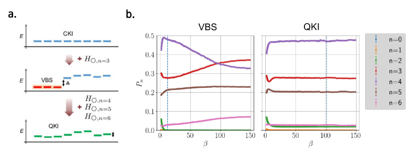
Figure 4: Effects of quantum tunnelling processes. a. The schematic picture of the energy level reorganization due to the sixth-order perturbation (6). Starting from the degenerate classical ice manifold, we first introduce the ring-exchange term $H_{\hexagon,n=3}$. This will select the three-fold degenerate VBS states with an energy gap $\Delta$. Further adding the diagonal terms $H_{\hexagon,n=4,5,6}$, the energy levels are reorganized to become quasi-degenerate with a suppressed energy gap. b. QMC results of the hexagon fraction $P_{n}$ v.s. $\beta$ in the VBS regime with $J_{\pm}=0.19$ and $J_{\pm\pm}=0$ (left panel); and in the QKI regime $J_{\pm\pm}=-0.49$ and $J_{\pm}=0$ (right panel). Both are under a field $h=J_{z}$. The vertical dashed lines indicate the perturbative energy scale estimated by the leading ring-exchange contribution with $\beta\sim 12.1/J_{z}$ and $\beta\sim 100.9/J_{z}$ for the left and right panel respectively.

Conclusions Although the XYZh model on a kagome lattice has been proposed to be a new playground to search for 2D $Z_{2}$ QSL, our results suggest that the QKI does not show a $Z_{2}$ topological order down to low temperature, and the system bahaves classically. The suppression of the quantum energy scale originated from the competition between the off-diagonal ring-exchange and diagonal processes indicates that a much lower temperature than $T=1/200$ has to be reached before entering the true quantum regime. Even if the true quantum ground state is a $Z_{2}$ QSL with an extremely small gap, it will be very hard to be realized experimentally or confirmed numerically since it is extremely fragile.

Our results also indicate that the kagome ice states cannot be hybridized easily with quantum anisotropic exchange. Thus, the kagome ice physics is more likely to be observed at finite temperature experiments with non-trivial dynamics. This non-perturbative result of QMC provides crucial information for understanding the experiments, such as the recent experiments on Nd₂Zr₂O₇ Lhotel et al. (2018). In addition to pyrochlore materials, such physics could also play a role in the recently synthesized tripod materials Paddison et al. (2016); Scheie et al. (2018); Dun et al. (2018).

On the other hand, although the true ground state remains unknown, it would be interesting to study the effects of tilting the field away from the [111] axis as this can provide an easy method to tune the weights of the ring-exchange and diagonal processes. We finish by pointing out the non-trivial diagonal terms we found through DPT also exist on the pyrochlore lattice since the CKI states are a subset of the ice manifold. Further systematic studies are necessary to see if the phenomena discussed in this paper can be extended to three-dimensional cases Rau and Gingras (2015); Huang et al. (2018).

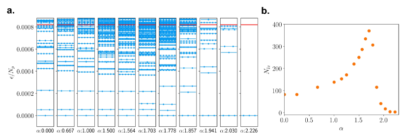
Figure 5: Spectrum of the effective Hamiltonian and effects of diagonal processes. (a) The energy spectrum of the effective model $\hat{P_{6}}$ with tuning parameter $\alpha$. Each dot represents a single state. The $y$-axis is the energy per-hexagon ($N_{p}=N/3$ is the number of hexagons), and each ground state is shifted to zero for easy comparison. The red line indicates an energy cutoff $\epsilon/N_{p}=0.00082$. (b) Number of energy levels, $N_{lv}$, that lies below the cutoff. $N_{lv}$ increases as $\alpha$ increases, indicating that the energy spectrum is compressed toward the ground state, until $\alpha>1.703$ where $N_{lv}$ decreases again.

II Methods

We implement the stochastic series expansion (SSE) Sandvik and Kurkijärvi (1991); Syljuasen and Sandvik (2002) in the $S^{z}$ basis with a triangular plaquette break-up of the XYZh Hamiltonian. The directed loop equations are solved using numerical linear solver to minimize the bounce probability. The Renyi entanglement entropy is measured by implementing the replica trick Isakov et al. (2011). In our simulations, we follow the scheme proposed in Ref. Melko et al. (2010) to measure the second Renyi entanglement entropy $S_{2}$ with four subregions independently. The simulation runs on average $10^{8}\sim 10^{9}$ Monte Carlo steps (MCS) for each subregion. The topological entanglement entropy $\gamma$ is calculated by combining $S_{2}$ of the four subregions with the standard bootstrap resampling procedure. The thermal entropy is measured with $10^{8}$ MCS using SSE with the Wang-Landau algorithm Troyer et al. (2004) for a long operator string with a fixed length. For the exact-diagonalisation of the effective Hamiltonian, we first search for all basis states that satisfy the 2-up-1-down ice-rule. We then construct the effective Hamiltonian $\hat{P}_{6}(\alpha)$, and perform a Lanczos diagonalisation to obtain the energy spectrum and eigenstates. The data presented in this paper requires the computation resources approximately about 330 CPU core-years on two different heterogeneous high-performance computers (HPCs) with 2.50GHz Intel Xeon or equivalent CPUs at the National Center for High-performance Computing.

Appendix A Degenerate perturbation theory

We start by identifying the classical part in the XYZh model as unperturbed system, denoting as $H_{0}$, and

$$H =H_{0}+V$$

$$H_{0} =J_{z}\sum_{\langle i,j\rangle}S^{i}_{z}S^{j}_{z}-h\sum_{i}S^{i}_{z}.$$ (9)

Next, we treat the quantum term $V$ as perturbation acting on the degenerate classical ice manifold $\bm{\Omega}=\{\Omega_{0},\Omega_{1},\ldots\}$ with the ice rule ”2-up-1-down” ($h>0$) or ”2-down-1-up” ($h<0$),

$$H_{0}\bm{\Omega} =E_{0}\bm{\Omega}.$$ (10)

Define an operator $\mathbb{P}$ that projects the states $\bm{\Psi}=\{\Psi_{0},\Psi_{1},\ldots\}$ in the Hilbert space to the degenerate ice manifold,

$$\mathbb{P}\bm{\Psi}=\bm{\Omega}$$ (11)

where $\mathbb{P}^{2}=\mathbb{P}$.

Following the standard Brillouin-Wigner perturbation theory Fulde (1995), the perturbation expansion can be written as Bergman et al. (2007a, b),

$$(H_{0}+\mathbb{P}V\sum_{t=0}^{\infty}G^{t}\mathbb{P})\bm{\Omega} =E\bm{\Omega}$$

$$G=\frac{(I-\mathbb{P})}{E-H_{0}}V.$$ (12)

We now have a non-linear eigenvalue problem to solve for the energy shifts ($\epsilon=E-E_{0}$),

$$\hat{P}\bm{\Omega}=\epsilon\bm{\Omega}$$ (13)

with

$$\hat{P}\equiv\left(V\sum_{t=0}^{\infty}G^{t}\right).$$ (14)

Essentially, perturbations coming from the quantum fluctuations lift the degeneracy of the ice manifold and quantum phase emerges. In the following calculation, we use hexagon units as defined in the main text and take $h>0$, where all the triangular plaques follows ”2-up-1-down” rule.

For the case that the $S^{\pm}S^{\pm}$ is the only present quantum fluctuation, the lowest non-constant term is at the sixth order,

$$VG^{5} \equiv\hat{P}_{6},$$ (15)

which is the sum of off-diagonal $H_{o}$ and diagonal $H_{d}$ contributions.

$$\hat{P}_{6} =H_{d}+H_{o}$$ (16)

$$H_{d} =D_{4,a}\sum_{\forall\hexagon n=4,a}H_{\hexagon}+D_{4,b}\sum_{\forall\hexagon n=4,b}H_{\hexagon}+D_{5}\sum_{\forall\hexagon n=5}H_{\hexagon}+D_{6}\sum_{\forall\hexagon n=6}H_{\hexagon}$$ (17)

$$H_{o} =K_{pp}\sum_{\forall\hexagon n=3}H_{\hexagon},$$ (18)

where the off-diagonal term corresponds to the ring-exchange process that acts on $n=3$ hexagons, and the diagonal terms correspond to processes that $V$ acts on each bond only once on $n\geq 4$ hexagons (see Fig. 6, 7, 8). Prefactors associated with each term can be computed by listing all possible ways to arrange the local two-site ($S^{\pm}S^{\pm}$ or $S^{\pm}S^{\mp}$) operators ($G$) to form the perturbation operators $H_{\hexagon}$ that transfer states within the ice manifold Bergman et al. (2007a, b).

The prefactors for the off-diagonal ring-exchange term,

$$K_{pp}=-\frac{6J^{6}_{\pm\pm}}{J_{z}^{2}(2h+J_{z})^{5}}\left[7J_{z}^{2}+14J_{z}h+8h^{2}\right]$$ (19)

and diagonal terms

$$D_{4,a} =-\frac{J^{6}_{\pm\pm}}{4hJ_{z}^{2}(J_{z}+2h)^{2}}$$

$$D_{4,b} =-\frac{(2J+h)J^{6}_{\pm\pm}}{4hJ_{z}^{2}(J_{z}+2h)^{2}(J-\frac{h}{2})}$$

$$D_{5} =-J^{6}_{\pm\pm}\frac{8J(3J_{z}+4h)(2J_{z}+h)+h(7J_{z}+4h)^{2}}{4hJ_{z}^{2}(J_{z}+2h)^{2}(2J_{z}+h)(3J_{z}+4h)^{2}}$$

$$D_{6} =-\frac{12J^{6}_{\pm\pm}}{(3J_{z}+4h)^{2}(J_{z}+2h)(J_{z}+h)h}.$$ (20)

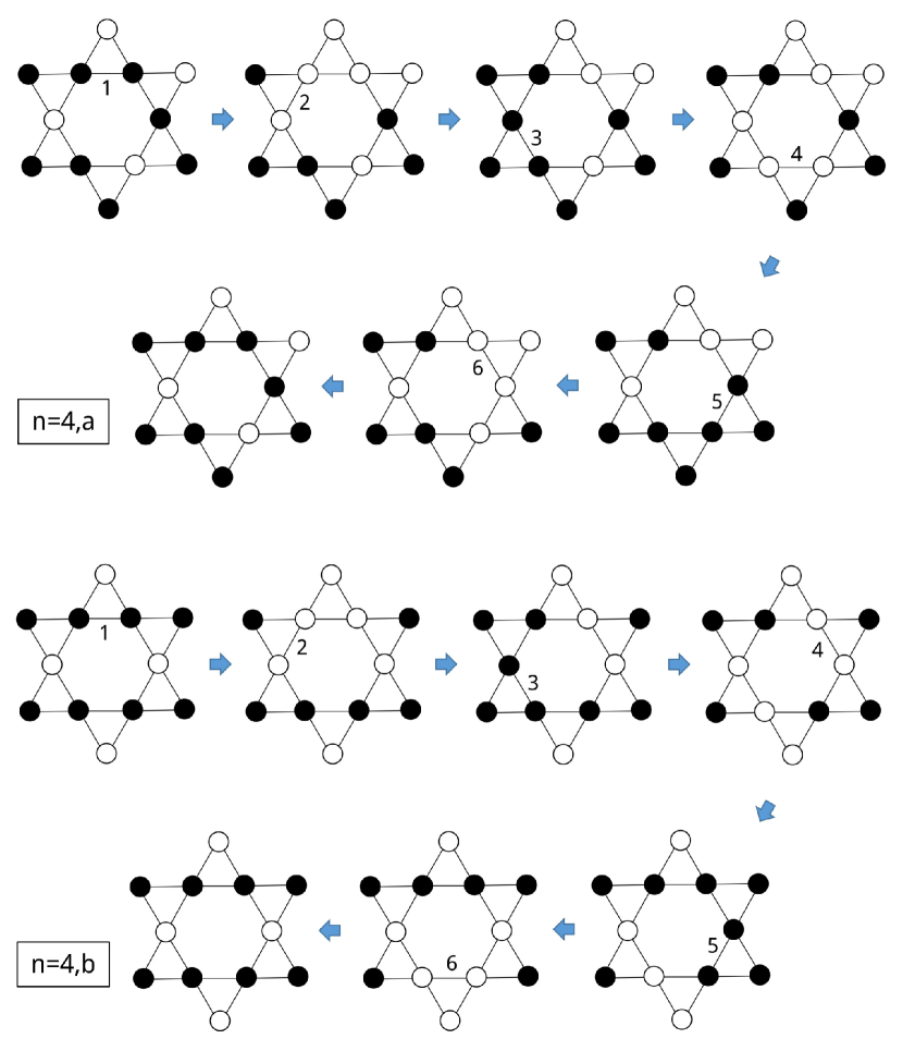
Figure 6: Relevant diagonal processes on two types of hexagon with $n=4$

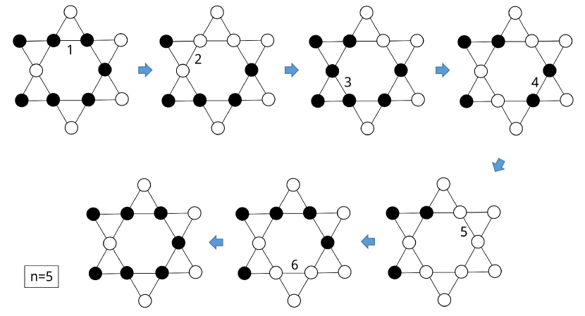
Figure 7: Relevant diagonal process on hexagon with $n=5$

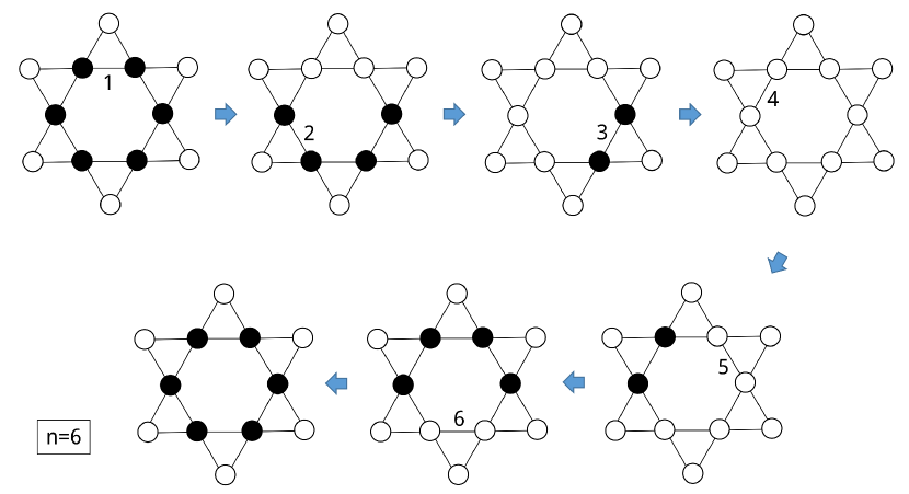
Figure 8: Relevant diagonal process on hexagon with $n=6$

If we further let $h=J_{z}$ provided the system is within the lobe, we obtain,

$$K_{pp} =-\frac{58}{81}\frac{J^{6}_{\pm\pm}}{J_{z}^{5}}$$

$$D_{4,a} =-\frac{1}{36}\frac{J^{6}_{\pm\pm}}{J_{z}^{5}}$$

$$D_{4,b} =-\frac{1}{6}\frac{J^{6}_{\pm\pm}}{J_{z}^{5}}$$

$$D_{5} =-\frac{289}{5292}\frac{J^{6}_{\pm\pm}}{J_{z}^{5}}$$

$$D_{6} =-\frac{2}{49}\frac{J^{6}_{\pm\pm}}{J_{z}^{5}}.$$ (21)

Appendix B Thermal entropy measurement using Wang-Landau method

In general, one can estimate thermal entropy by numerically integrating the specific heat data from QMC. However, this approach requires a very accurate estimate of the specific heat and suffers from the error due to the discretized temperature intervals. Instead, we use the Wang-Landau sampling scheme Troyer et al. (2004) to directly access the thermal entropy in our QMC simulations.

In the SSE formalism, the partition function is written as

$$Z =\textrm{Tr}{\left[e^{-\beta H}\right]}$$

$$=\sum_{n}\frac{(\beta)^{n}}{n!}\sum_{\phi,a,b}\bra{\phi}H_{a_{0},b_{0}}...H_{a_{n},b_{n}}\ket{\phi}$$

$$=\sum_{n}\beta^{n}S_{n}$$

$$=\sum_{n}W(n),$$ (22)

where $H_{a_{i},b_{i}}$ is the local Hamiltonian. In our simulation, we perform triangle plaquette decomposition of the Hamiltonian as discussed in Ref. Melko (2007) and sampling using the directed loop algorithm Syljuasen and Sandvik (2002). Here, we rewrite Eq. (22) into a generalized representation by introducing a weighting factor $g(n)$,

$$Z^{\prime} =\sum_{n}\beta^{n}S_{n}\ g(n)$$

$$=\sum_{n}W^{\prime}(n).$$ (23)

In the simulation, we first search for $g(n)$ such that the modified weight $W^{\prime}(n)$ are roughly equal, and then sample $Z^{\prime}$ with the modified weight $W^{\prime}(n)$.

The partition function for a range of arbitrary temperatures $\bar{\beta}$ can be calculated by,

$$Z(\bar{\beta})=\sum_{n}\left(\frac{\bar{\beta}}{\beta}\right)^{n}\frac{W^{\prime}(n)}{g(n)}.$$ (24)

In our simulation, we fix $\beta=1$ for convenience. To obtain the estimates for physical observables, we first record the estimates for each observables in each $n$ separately,

$$\langle O_{n}\rangle =\sum_{n^{\prime}}O\delta_{n,n^{\prime}}\frac{W^{\prime}(n^{\prime})}{Z^{\prime}}$$

$$\langle I_{n}\rangle =\delta_{n,n^{\prime}}\frac{W^{\prime}(n^{\prime})}{Z^{\prime}}.$$ (25)

We then reweight the estimates with the set $\{g(n)\}$ with an undetermined normalization constant $A$,

$$\langle\bar{O}(\bar{\beta})\rangle =A\sum_{n}\frac{(\bar{\beta})^{n}}{g(n)}\langle O_{n}\rangle$$

$$\langle\bar{Z}(\bar{\beta})\rangle =A\sum_{n}\frac{(\bar{\beta})^{n}}{g(n)}\langle I_{n}\rangle.$$ (26)

The observables with arbitrary $\bar{\beta}$ can be obtained with the relation,

$$\langle O(\bar{\beta})\rangle=\frac{\langle\bar{O}(\bar{\beta})\rangle}{\langle\bar{Z}(\bar{\beta})\rangle}.$$ (27)

To determine $A$, we use the fact that the $n=0$ sector corresponds to a system at infinite temperature ($\beta\rightarrow 0$),

$$A\frac{\langle I_{0}\rangle}{g(0)}=2^{N},$$ (28)

where $N$ is the total number of spins in the system. Using this relation, the physical partition function, free energy and entropy can be calculated,

$$\langle Z(\bar{\beta})\rangle =\sum_{n}(\bar{\beta})^{n}\frac{I_{n}}{I_{0}}\frac{g(0)}{g(n)}2^{N},$$ (29)

$$\langle F(\bar{\beta})\rangle =-\frac{1}{\bar{\beta}}\ln\left[\langle Z(\bar{\beta})\rangle\right],$$ (30)

$$\langle S(\bar{\beta})\rangle =\bar{\beta}\left[E(\bar{\beta})-F(\bar{\beta})\right].$$ (31)

Appendix C Topological entanglement entropy and Levin-Wen construction

As shown in the main text, in order to identify the $Z_{2}$ QSL, we have to numerically compute the topological entanglement entropy (TEE). In our simulation, we use the second Renyi entropy $S_{2}$ as our entanglement measurement. The Renyi entropy with sub-region $A$ follows the area law,

$$S_{A}=\kappa l-\eta\gamma+O(L^{-1})$$ (32)

where $l$ is the boundary of the sub-region $A$ and $\gamma$ is the topological entanglement entropy. Here, we also consider a finite size correction $O(L^{-1})$ that goes to zero in the thermodynamic limit.

The Renyi entropy is computed using QMC following the procedure in Ref. Melko et al. (2010). Application of this method to identify the $Z_{2}$ topological order can be found in Ref. Isakov et al. (2011). To estimate the topological entanglement entropy, we use the Levin-Wen construction  Levin and Wen (2006) to eliminate the contributions from the boundaries (area law term). We first construct four different parts out of the lattice; marked by $A$, $B$, $C$ and $D$ as shown in Fig. 9.

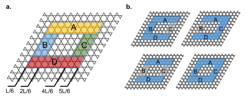
Figure 9: Levin-Wen construction. a. Four small parts $A$, $B$, $C$ and $D$ in the system with size $L$. b. Four different sub-regions $R_{1}$ (upper-left), $R_{2}$ (upper-right), $R_{3}$ (lower-left) and $R_{4}$ (lower-right) are constructed from the four parts $A$, $B$, $C$ and $D$ in order to eliminate the contribution from the boundaries.

We then strategically construct four different sub-regions $R_{1}$, $R_{2}$, $R_{3}$ and $R_{4}$ with different combination of these four parts as

$$R_{1} =A\cup B\cup D,$$

$$R_{2} =A\cup C\cup D,$$

$$R_{3} =A\cup D,$$

$$R_{4} =A\cup B\cup C\cup D.$$

The choice for these subregions allows one to extract the topological entanglement entropy $\gamma$ using the relation

$$2\gamma=-S_{2}(R_{1})-S_{2}(R_{2})+S_{2}(R_{3})+S_{2}(R_{4})$$

to eliminate the contributions coming from the boundaries Levin and Wen (2006).

Appendix D Hexagon fraction for $J_{\pm}\neq 0$ and $J_{\pm\pm}\neq 0$

Here we present the hexagon fraction for the case $J_{\pm}\neq 0$ and $J_{\pm\pm}\neq 0$ where a VBS ground state is expected to establish based on our degenerate perturbation theory analysis. In Fig. 10 we show the QMC results of hexagon fractions $P_{n}$ at $h=J_{z}$, $J_{\pm}=0.1219J_{z}$ and $J_{\pm\pm}=-0.25J_{z}$. The parameters lie in the VBS region with a dominant ring-exchange term as the third-order perturbation (as also presented in Fig. 11b). Our result clearly shows the rise of $P_{3}$ and the decrease of $P_{4}$ at temperature lower than the perturbative energy scale estimated by the ring-exchange process $\beta\sim\frac{J_{z}^{2}}{12J_{\pm}^{3}}=46/J_{z}$, with the same behaviour as in the XXZ model ($J_{\pm}\neq 0$, $J_{\pm\pm}=0$). This should be contrasted with the behaviour of Fig. 4b in the main text.

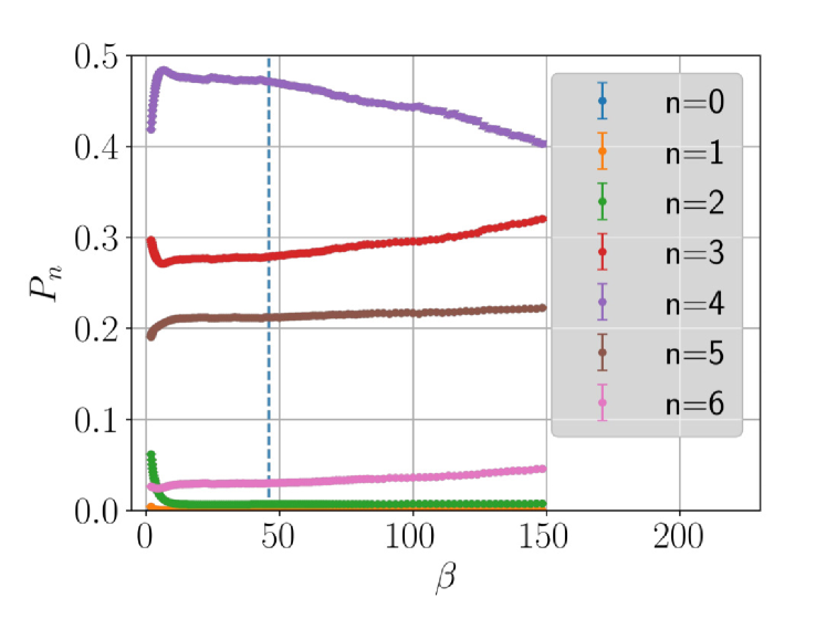
Figure 10: Hexagon occupation fraction. The hexagon fraction in the VBS region with $h=J_{z}$, $J_{\pm}=0.1219J_{z}$ and $J_{\pm\pm}=-0.25J_{z}$. The vertical blue line indicates the perturbative energy scale

Appendix E Phase diagrams and Structure factors

In Fig. 11 we show a general phase diagram of XYZh model in parameter space $J_{\pm}-J_{\pm\pm}-h$. In the figure, projections to the $J_{\pm}=0$ and $J_{\pm\pm}=0$ planes are shown with the simulation data. To map out the phase boundaries, we take the advantage of the sudden change of the magnetization $M_{z}$ and magnetic susceptibility $\chi_{z}$ across the transition to identify the phase boundaries. The magnetization $M_{z}$ and magnetic susceptibility $\chi_{z}$ are defined as

$$M_{z} =\frac{1}{N}\left\langle\sum_{i}S^{z}_{i}\right\rangle,$$

$$\chi_{z} =\left\langle\left(\sum_{i}S^{z}_{i}\right)^{2}\right\rangle-\left\langle\sum_{i}S^{z}_{i}\right\rangle^{2}.$$ (33)

Fig. 12 shows the phase diagrams of various cross section of the parameter space. For plane with $J_{\pm}=0$, two phases of QKI and ferromagnetic (FM) are identified, which is consistent with previous study  Carrasquilla et al. (2015). For plane with $J_{\pm\pm}=0$, we have VBS and superfluid (SF) phase as  Isakov et al. (2006).

At $J_{\pm}-J_{\pm\pm}$ plane with a horizontal cross section at $h=1.0$, we find a lobe with VBS ordering at a finite $J_{\pm}$. The emergence of VBS is consistent and expected as a consequences of introducing a third order ring-exchange term that is shown in our DPT analysis.

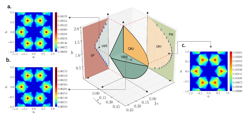
Figure 11: Phase diagram and structure factors. The schematic phase diagram shows possible phases of the XYZh model. The phase boundaries are guides to the eye. For $J_{\pm}=0$ plane, two phases of QKI and ferromagnetic (FM) ordered phase are identified as also shown in Fig. 12b. For $J_{\pm\pm}=0$ plane, the lobe of VBS phase appears at $J_{\pm}\ll 1$. The system enters the super fluid phase (SF) when increasing the hopping term $J_{\pm}$ as also shown in Fig. 12a. Structure factors for three cases with a. $J_{\pm\pm}=0$ , $J_{\pm}=0.19$ and $h=1.0$, b. $J_{\pm\pm}=-0.25$ , $J_{\pm}=0.1219$ , $h=1.0$, and c. $J_{\pm\pm}=-0.45$ , $J_{\pm}=0$ and $h=1.0$. In cases a and b, peaks are observed at $\bm{Q}=\left\langle\frac{2\pi}{3},0\right\rangle$ and symmetry related momenta, indicating the emergence of the VBS order; while in the QKI phase (case c), no such peak is observed. The structure factors are measured with system size $L=12$ at $T=0.02$. The momentum vectors $q_{x}$ and $q_{y}$ are in unit of $2\pi$ with ferromagnetic peaks being removed for clarity.

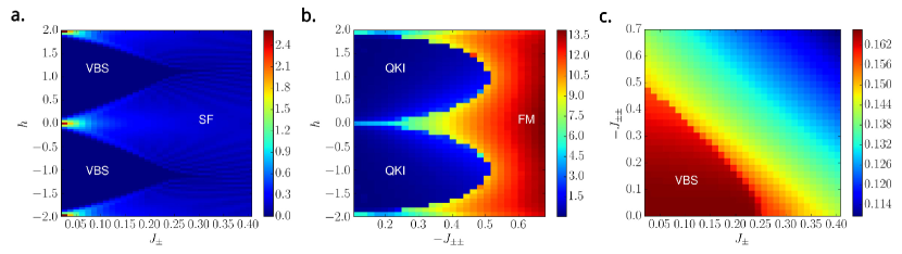
Figure 12: Phase diagram in various planes of the parameter space. a. Phase diagram in the $J_{\pm}$-$h$ plane. b. Phase diagram in the $J_{\pm\pm}-h$ plane. c. Phase diagram in the $J_{\pm}-J_{\pm\pm}$ plane with $h=1$. Simulations are performed with system size $L=6$ at temperature $T=0.015J_{z}$ using standard SSE. For a. and .b, the phase diagram are mapped by the magnetic susceptibility $\chi_{z}$. For (c), the phase diagram is mapped by the magnetization $M_{z}$.

The three-fold degenerate VBS state with broken translational symmetry can be identified from the peaks of the static structure factor $S(\mathbf{q})$ at ordering momentum vector $\mathbf{q}=\left\langle\frac{2\pi}{3},0\right\rangle$ and symmetry related momenta Isakov et al. (2006). The static structure factor defines as :

$$f(\mathbf{q}) =\frac{1}{N}\sum_{j}e^{i\mathbf{q}\cdot\mathbf{r}_{j}}S^{z}_{j}$$

$$S(\mathbf{q}) =\left\langle f(\mathbf{q})f(-\mathbf{q})\right\rangle-\left\langle f(\mathbf{q})\right\rangle\left\langle f(-\mathbf{q})\right\rangle$$ (34)

with $N=3\times L\times L$ is the total number of spins. Fig. 13 shows the line cut along $\mathbf{q}=(q_{x},0)$ of the structure factors shown in Fig. 11. In both the VBS-a and VBS-b cases, peaks at $\mathbf{q}=\left\langle\frac{2\pi}{3},0\right\rangle$ emerge out of the background.

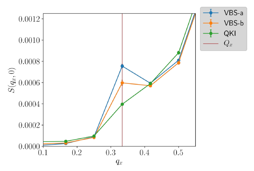
Figure 13: Structure factors in various phases. The structure factors are measured at $N=3\times 12\times 12$ at $T=0.02$. The curves of VBS-a, VBS-b and QKI correspond to the line cut along $\mathbf{q}=(q_{x},0)$ of Fig. 11a, Fig. 11b and Fig. 11c respectively. The $x$ component momentum vector $q_{x}$ are in units of $2\pi$. $Q_{x}=\frac{2\pi}{3}$ indicates the VBS ordering vector.

Appendix F Ground states of the modified effective model

To understand the ground states of the modified effective model, we analyse the spectral properties of the energy eigenstates $\ket{\phi_{i}}$ obtained by exact diagonalisation. We write the state of interest $\ket{\phi_{i}}$ in terms of the classical kagome ice basis $\{\Omega_{n}\}$ where the energy eigenstate $\ket{\phi_{i}}$ can be represented as:

$$\ket{\phi_{i}}=\sum_{n}A_{n}\ket{\Omega_{n}},\quad C_{n}\equiv\left|A_{n}\right|^{2},$$ (35)

where $C_{n}$ corresponds to the probability of the classical state $\Omega_{n}$.

We first study the effective model in the classical limit with only the diagonal term Eq. (17) present. This amounts to taking $\alpha\to\infty$ in the original $\hat{P}_{6}$ model in the main text.

Fig. 14a shows the energy spectrum and we find the ground states are three-fold degenerate. These states are linear combination of three possible charge-ordered states in the classical kagome ice Chern et al. (2011); Wolf and Schotte (1988) (Fig. 14b), marked with $\mathrm{I}$, $\mathrm{II}$ and $\mathrm{III}$ shown in Fig. 14c. Note that every hexagons within these charge-ordered configurations are all $n=4,b$. These states are smoothly connected to the ground states for $\alpha\gtrsim 1.703$.

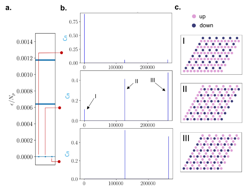
Figure 14: Energy spectrum of the diagonal-only model. a. The spectrum of the effective model (17) with only the diagonal terms for $N=6\times 6\times 3$, $J_{\pm\pm}=-0.49,h=1.0,J_{\pm}=0$. $N_{p}=N/3$ is the number of hexagons. The ground energy is shifted to zero. b. The three-fold degenerate ground states represented in the classical kagome ice states. The blue bar represents the probability $C_{n}$ for each configuration and the $x$-axis is the classical configuration index.where $x$-axis is the classical configuration index. The ground states corresponds to linear combination of three charge-ordered states in classical kagome ice c..

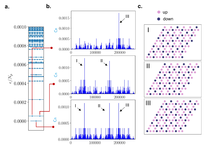
Figure 15: Energy spectrum of the ring-exchange model. a. The spectrum of the ring-exchange model Eq. (18). The ground energy is shifted to zero. The system size is $N=6\times 6\times 3$ and $N_{p}=N/3$ is the number of hexagons. b. The three lowest energy eigenstates represented in the classical kagome ice states. The blue bar represents the probability $C_{n}$ for each configuration and the $x$-axis is the classical configuration index. c. Three ice configurations with dominant probabilities $C_{n}$ for the three lowest energy states. The classical configurations correspond to the $\sqrt{3}\times\sqrt{3}$ states. The parameters considered here are $J_{\pm\pm}=-0.49,h=1.0,J_{\pm}=0$.

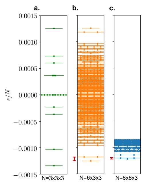
Figure 16: The energy spectrums of different system sizes. The full spectrum the effective model at $\alpha=0$ for systems with total number of spins $N=3\times 3\times 3$ (a) , and $N=6\times 3\times 3$ (b) , and the lowest 300 states for system $N=6\times 6\times 3$ (c). The finite-size gap between the ground states and the first-excited state, indicated by the red line, decreases as the system size increases. The parameters are $J_{\pm\pm}=-0.49,h=1.0,J_{\pm}=0$.

In the other limit $\alpha=0$, where only the ring-exchange term Eq. (18) is present, we expect a three-fold degenerate VBS ground state Isakov et al. (2006); Moessner et al. (2001) in the thermodynamic limit. In a finite-size simulation, these states are not exactly degenerate. However, the spectral property of these states should manifest the VBS signature. Fig. 15a shows the energy spectrum of the ring-exchange model. The three lowest energy states ( Fig. 15b) are the linear superposition of classical configurations with $n=3$ hexagons, dominated by three configurations corresponding configurations to the $\sqrt{3}\times\sqrt{3}$ states as shown in Fig. 15c. The VBS states are generated by the tunnelling between these three $\sqrt{3}\times\sqrt{3}$ states with the ring-exchange, and other $n=3$ states are intermediate configurations generated from the tunnelling processes. These states are smoothly connected to the lowest energy states for $\alpha\lesssim 1.703$.

Finally, to show the three lowest states will eventually combined to form the three-fold degenerate states in the thermodynamic limit, we compare the finite-size gap for different system sizes as shown in Fig. 16. We see that the gap between the lowest three states decreases as system size increases, and the states become degenerate in the thermodynamic limit.

References

- Prange and Girvin (1990.) Richard E. Prange and Steven M. Girvin, The Quantum Hall effect, 2nd ed. (Springer-Verlag,, New York, 1990.).
- Tang et al. (2011) Evelyn Tang, Jia-Wei Mei, and Xiao-Gang Wen, “High-temperature fractional quantum hall states,” Phys. Rev. Lett. 106, 236802 (2011).
- Neupert et al. (2011) Titus Neupert, Luiz Santos, Claudio Chamon, and Christopher Mudry, “Fractional quantum hall states at zero magnetic field,” Phys. Rev. Lett. 106, 236804 (2011).
- Sun et al. (2011) Kai Sun, Zhengcheng Gu, Hosho Katsura, and S. Das Sarma, “Nearly flatbands with nontrivial topology,” Phys. Rev. Lett. 106, 236803 (2011).
- Anderson (1973) Philip W. Anderson, “Resonating valence bonds: A new kind of insulator?” Materials Research Bulletin 8, 153 (1973).
- Anderson (1987) Philip W. Anderson, “The resonating valence bond state in and superconductivity,” Science 235, 1196 (1987).
- Moessner and Sondhi (2001a) R. Moessner and S. L. Sondhi, “Resonating valence bond phase in the triangular lattice quantum dimer model,” Phys. Rev. Lett. 86, 1881–1884 (2001a).
- Gingras and McClarty (2014) Michel J. P. Gingras and P. A. McClarty, “Quantum spin ice: a search for gapless quantum spin liquids in pyrochlore magnets,” Reports on Progress in Physics 77, 056501 (2014).
- Zhou et al. (2017) Yi Zhou, Kazushi Kanoda, and Tai-Kai Ng, “Quantum spin liquid states,” Rev. Mod. Phys. 89, 025003 (2017).
- Savary and Balents (2017a) Lucile Savary and Leon Balents, “Quantum spin liquids: a review,” Reports on Progress in Physics 80, 016502 (2017a).
- Knolle and Moessner (2018) J. Knolle and R. Moessner, “A Field Guide to Spin Liquids,” (2018), arXiv:1804.02037 [cond-mat.str-el] .
- Gardner et al. (2010) Jason S. Gardner, Michel J. P. Gingras, and John E. Greedan, “Magnetic pyrochlore oxides,” Rev. Mod. Phys. 82, 53–107 (2010).
- Hermele et al. (2004) Michael Hermele, Matthew P. A. Fisher, and Leon Balents, “Pyrochlore photons: The spin liquid in a three-dimensional frustrated magnet,” Phys. Rev. B 69, 064404 (2004).
- Savary and Balents (2012) Lucile Savary and Leon Balents, “Coulombic quantum liquids in spin- pyrochlores,” Phys. Rev. Lett. 108, 037202 (2012).
- Lee et al. (2012) SungBin Lee, Shigeki Onoda, and Leon Balents, “Generic quantum spin ice,” Phys. Rev. B 86, 104412 (2012).
- Shannon et al. (2012) Nic Shannon, Olga Sikora, Frank Pollmann, Karlo Penc, and Peter Fulde, “Quantum ice: A quantum monte carlo study,” Phys. Rev. Lett. 108, 067204 (2012).
- Huang et al. (2014) Yi-Ping Huang, Gang Chen, and Michael Hermele, “Quantum spin ices and topological phases from dipolar-octupolar doublets on the pyrochlore lattice,” Phys. Rev. Lett. 112, 167203 (2014).
- Kato and Onoda (2015) Yasuyuki Kato and Shigeki Onoda, “Numerical evidence of quantum melting of spin ice: Quantum-to-classical crossover,” Phys. Rev. Lett. 115, 077202 (2015).
- Li et al. (2016) Yao-Dong Li, Xiaoqun Wang, and Gang Chen, “Hidden multipolar orders of dipole-octupole doublets on a triangular lattice,” Phys. Rev. B 94, 201114 (2016).
- Li and Chen (2017) Yao-Dong Li and Gang Chen, “Symmetry enriched U(1) topological orders for dipole-octupole doublets on a pyrochlore lattice,” Phys. Rev. B 95, 041106 (2017).
- Savary and Balents (2017b) Lucile Savary and Leon Balents, “Disorder-induced quantum spin liquid in spin ice pyrochlores,” Phys. Rev. Lett. 118, 087203 (2017b).
- Carrasquilla et al. (2015) Juan Carrasquilla, Zhihao Hao, and R. G. Melko, “A two-dimensional spin liquid in quantum kagome ice,” Nature communications 6, 7421 (2015).
- Scheie et al. (2018) A. Scheie, M. Sanders, J. Krizan, A. D. Christianson, V. O. Garlea, R. J. Cava, and C. Broholm, “Crystal field levels and magnetic anisotropy in the kagome compounds , , and ,” (2018), arXiv:1808.05111 [cond-mat.str-el] .
- Isakov et al. (2006) S. V. Isakov, S. Wessel, R. G. Melko, K. Sengupta, and Yong Baek Kim, “Hard-core bosons on the kagome lattice: Valence-bond solids and their quantum melting,” Phys. Rev. Lett. 97, 147202 (2006).
- Damle and Senthil (2006) Kedar Damle and T. Senthil, “Spin nematics and magnetization plateau transition in anisotropic kagome magnets,” Phys. Rev. Lett. 97, 067202 (2006).
- Huang and Hermele (2017) Yi-Ping Huang and Michael Hermele, “Theory of quantum kagome ice and vison zero modes,” Phys. Rev. B 95, 075130 (2017).
- Kitaev and Preskill (2006) Alexei Kitaev and John Preskill, “Topological entanglement entropy,” Phys. Rev. Lett. 96, 110404 (2006).
- Levin and Wen (2006) Michael Levin and Xiao-Gang Wen, “Detecting topological order in a ground state wave function,” Phys. Rev. Lett. 96, 110405 (2006).
- Rowell et al. (2009) Eric Rowell, Richard Stong, and Zhenghan Wang, “On classification of modular tensor categories,” Communications in Mathematical Physics 292, 343–389 (2009).
- Jiang et al. (2012) Hong-Chen Jiang, Zhenghan Wang, and Leon Balents, “Identifying topological order by entanglement entropy,” Nature Physics 8, 902 (2012).
- Isakov et al. (2011) Sergei V. Isakov, Matthew B. Hastings, and Roger G. Melko, “Topological entanglement entropy of a Bose-Hubbard spin liquid,” Nature Physics 7, 772 (2011).
- Cirac et al. (2011) J. Ignacio Cirac, Didier Poilblanc, Norbert Schuch, and Frank Verstraete, “Entanglement spectrum and boundary theories with projected entangled-pair states,” Phys. Rev. B 83, 245134 (2011).
- Moessner and Sondhi (2001b) R. Moessner and S. L. Sondhi, “Ising models of quantum frustration,” Phys. Rev. B 63, 224401 (2001b).
- Troyer et al. (2004) Matthias Troyer, Fabien Alet, and Stefan Wessel, “Histogram methods for quantum systems: from reweighting to Wang-Landau sampling,” Brazilian Journal of Physics 34, 377 – 383 (2004).
- Villain et al. (1980) J. Villain, R. Bidaux, J.-P. Carton, and R. Conte, “Order as an effect of disorder,” Journal de Physique 41, 1263–1272 (1980).
- Savary et al. (2012) Lucile Savary, Kate A. Ross, Bruce D. Gaulin, Jacob P. C. Ruff, and Leon Balents, “Order by quantum disorder in ,” Phys. Rev. Lett. 109, 167201 (2012).
- Zhitomirsky et al. (2012) M. E. Zhitomirsky, M. V. Gvozdikova, P. C. W. Holdsworth, and R. Moessner, “Quantum order by disorder and accidental soft mode in ,” Phys. Rev. Lett. 109, 077204 (2012).
- Bergman et al. (2007a) Doron L Bergman, Ryuichi Shindou, Gregory A Fiete, and Leon Balents, “Effective hamiltonians for some highly frustrated magnets,” Journal of Physics: Condensed Matter 19, 145204 (2007a).
- Bergman et al. (2007b) Doron L. Bergman, Ryuichi Shindou, Gregory A. Fiete, and Leon Balents, “Degenerate perturbation theory of quantum fluctuations in a pyrochlore antiferromagnet,” Phys. Rev. B 75, 094403 (2007b).
- Chern et al. (2011) Gia-Wei Chern, Paula Mellado, and O. Tchernyshyov, “Two-stage ordering of spins in dipolar spin ice on the kagome lattice,” Phys. Rev. Lett. 106, 207202 (2011).
- Wolf and Schotte (1988) M Wolf and K D Schotte, “Ising model with competing next-nearest-neighbour interactions on the kagome lattice,” Journal of Physics A: Mathematical and General 21, 2195 (1988).
- Lhotel et al. (2018) E. Lhotel, S. Petit, M. Ciomaga Hatnean, J. Ollivier, H. Mutka, E. Ressouche, M. R. Lees, and G. Balakrishnan, “Evidence for dynamic kagome ice,” Nature Communications 9, 3786 (2018).
- Paddison et al. (2016) Joseph A. M. Paddison, Harapan S. Ong, James O. Hamp, Paromita Mukherjee, Xiaojian Bai, Matthew G. Tucker, Nicholas P. Butch, Claudio Castelnovo, Martin Mourigal, and S. E. Dutton, “Emergent order in the kagome ising magnet Dy3Mg2Sb3O14,” Nature Communications 7, 13842 EP – (2016).
- Dun et al. (2018) Z. Dun, X. Bai, J. A. M. Paddison, N. P. Butch, C. D. Cruz, M. B. Stone, T. Hong, M. Mourigal, and H. Zhou, “Quantum spin fragmentation in kagome ice ,” (2018), arXiv:1806.04081 [cond-mat.str-el] .
- Rau and Gingras (2015) Jeffrey G. Rau and Michel J. P. Gingras, “Magnitude of quantum effects in classical spin ices,” Phys. Rev. B 92, 144417 (2015).
- Huang et al. (2018) C.-J. Huang, C. Liu, Z. Meng, Y. Yu, Y. Deng, and G. Chen, “Extended Coulomb liquid of paired hardcore boson model on a pyrochlore lattice,” (2018), arXiv:1806.04014 [cond-mat.str-el] .
- Sandvik and Kurkijärvi (1991) Anders W. Sandvik and Juhani Kurkijärvi, “Quantum Monte Carlo simulation method for spin systems,” Phys. Rev. B 43, 5950–5961 (1991).
- Syljuasen and Sandvik (2002) Olav F. Syljuasen and Anders W. Sandvik, “Quantum Monte Carlo with directed loops,” Phys. Rev. E 66, 046701 (2002).
- Melko et al. (2010) Roger G. Melko, Ann B. Kallin, and Matthew B. Hastings, “Finite-size scaling of mutual information in Monte Carlo simulations: Application to the spin- XXZ model,” Phys. Rev. B 82, 100409 (2010).
- Fulde (1995) Peter Fulde, Electron correlations in molecules and solids, 3rd ed., Springer series in solid-state sciences ; 100 (Springer-Verlag, Berlin ; New York, 1995).
- Melko (2007) Roger G Melko, “Simulations of quantum XXZ models on two-dimensional frustrated lattices,” Journal of Physics: Condensed Matter 19, 145203 (2007).
- Moessner et al. (2001) R. Moessner, S. L. Sondhi, and P. Chandra, “Phase diagram of the hexagonal lattice quantum dimer model,” Phys. Rev. B 64, 144416 (2001).