Sliced-Wasserstein Flows: Nonparametric Generative Modeling via Optimal Transport and Diffusions

Sliced-Wasserstein Flows: Nonparametric Generative Modeling via Optimal Transport and Diffusions
SUPPLEMENTARY DOCUMENT

Abstract

By building upon the recent theory that established the connection between implicit generative modeling (IGM) and optimal transport, in this study, we propose a novel parameter-free algorithm for learning the underlying distributions of complicated datasets and sampling from them. The proposed algorithm is based on a functional optimization problem, which aims at finding a measure that is close to the data distribution as much as possible and also expressive enough for generative modeling purposes. We formulate the problem as a gradient flow in the space of probability measures. The connections between gradient flows and stochastic differential equations let us develop a computationally efficient algorithm for solving the optimization problem. We provide formal theoretical analysis where we prove finite-time error guarantees for the proposed algorithm. To the best of our knowledge, the proposed algorithm is the first nonparametric IGM algorithm with explicit theoretical guarantees. Our experimental results support our theory and show that our algorithm is able to successfully capture the structure of different types of data distributions.

1 Introduction

Implicit generative modeling (IGM) (Diggle & Gratton, 1984; Mohamed & Lakshminarayanan, 2016) has become very popular recently and has proven successful in various fields; variational auto-encoders (VAE) (Kingma & Welling, 2013) and generative adversarial networks (GAN) (Goodfellow et al., 2014) being its two well-known examples. The goal in IGM can be briefly described as learning the underlying probability measure of a given dataset, denoted as $\nu\in{\cal P}(\Omega)$, where ${\cal P}$ is the space of probability measures on the measurable space $(\Omega,\mathcal{A})$, $\Omega\subset\mathbb{R}^{d}$ is a domain and $\mathcal{A}$ is the associated Borel $\sigma$-field.

Given a set of data points $\{y_{1},\dots,y_{P}\}$ that are assumed to be independent and identically distributed (i.i.d.) samples drawn from $\nu$, the implicit generative framework models them as the output of a measurable map, i.e. $y=T(x)$, with $T:\Omega_{\mu}\mapsto\Omega$. Here, the inputs $x$ are generated from a known and easy to sample source measure $\mu$ on $\Omega_{\mu}$ (e.g. Gaussian or uniform measures), and the outputs $T(x)$ should match the unknown target measure $\nu$ on $\Omega$.

Learning generative networks have witnessed several groundbreaking contributions in recent years. Motivated by this fact, there has been an interest in illuminating the theoretical foundations of VAEs and GANs (Bousquet et al., 2017; Liu et al., 2017). It has been shown that these implicit models have close connections with the theory of Optimal Transport (OT) (Villani, 2008). As it turns out, OT brings new light on the generative modeling problem: there have been several extensions of VAEs (Tolstikhin et al., 2017; Kolouri et al., 2018) and GANs (Arjovsky et al., 2017; Gulrajani et al., 2017; Guo et al., 2017; Lei et al., 2017), which exploit the links between OT and IGM.

OT studies whether it is possible to transform samples from a source distribution $\mu$ to a target distribution $\nu$. From this perspective, an ideal generative model is simply a transport map from $\mu$ to $\nu$. This can be written by using some ‘push-forward operators’: we seek a mapping $T$ that ‘pushes $\mu$ onto $\nu$’, and is formally defined as $\nu(A)=\mu(T^{-1}(A))$ for all Borel sets $A\subset\mathcal{A}$. If this relation holds, we denote the push-forward operator $T_{\#}$, such that $T_{\#}\mu=\nu$. Provided mild conditions on these distributions hold (notably $\mu$ is non-atomic (Villani, 2008)), existence of such a transport map is guaranteed; however, it remains a challenge to construct it in practice.

One common point between VAE and GAN is to adopt an approximate strategy and consider transport maps that belong to a parametric family $T_{\phi}$ with $\phi\in\Phi$. Then, they aim at finding the best parameter $\phi^{\star}$ that would give $T_{\phi^{\star}\#}\mu\approx\nu$. This is typically achieved by attempting to minimize the following optimization problem: $\phi^{\star}=\operatorname*{arg\min}_{\phi\in\Phi}{\cal W}_{2}(T_{\phi\#}\mu,\nu)$, where ${\cal W}_{2}$ denotes the Wasserstein distance that will be properly defined in Section 2. It has been shown that (Genevay et al., 2017) OT-based GANs (Arjovsky et al., 2017) and VAEs (Tolstikhin et al., 2017) both use this formulation with different parameterizations and different equivalent definitions of ${\cal W}_{2}$. However, their resulting algorithms still lack theoretical understanding.

In this study, we follow a completely different approach for IGM, where we aim at developing an algorithm with explicit theoretical guarantees for estimating a transport map between source $\mu$ and target $\nu$. The generated transport map will be nonparametric (in the sense that it does not belong to some family of functions, like a neural network), and it will be iteratively augmented: always increasing the quality of the fit along iterations. Formally, we take $T_{t}$ as the constructed transport map at time $t\in[0,\infty)$, and define $\mu_{t}=T_{t}\#\mu$ as the corresponding output distribution. Our objective is to build the maps so that $\mu_{t}$ will converge to the solution of a functional optimization problem, defined through a gradient flow in the Wasserstein space. Informally, we will consider a gradient flow that has the following form:

$$\partial_{t}\mu_{t}=-\nabla_{{\cal W}_{2}}\Bigl{\{}\mathrm{Cost}(\mu_{t},\nu)+\mathrm{Reg}(\mu_{t})\Bigr{\}}\,,\>\>\mu_{0}=\mu,$$ (1)

where the functional $\mathrm{Cost}$ computes a discrepancy between $\mu_{t}$ and $\nu$, $\mathrm{Reg}$ denotes a regularization functional, and $\nabla_{{\cal W}_{2}}$ denotes a notion of gradient with respect to a probability measure in the ${\cal W}_{2}$ metric for probability measures. If this flow can be simulated, one would hope for $\mu_{t}=(T_{t})_{\#}\mu$ to converge to the minimum of the functional optimization problem: $\min_{\mu}(\mathrm{Cost}(\mu,\nu)+\mathrm{Reg}(\mu))$ (Ambrosio et al., 2008; Santambrogio, 2017).

We construct a gradient flow where we choose the $\mathrm{Cost}$ functional as the sliced Wasserstein distance (${\cal S}{\cal W}_{2}$) (Rabin et al., 2012; Bonneel et al., 2015) and the $\mathrm{Reg}$ functional as the negative entropy. The ${\cal S}{\cal W}_{2}$ distance is equivalent to the ${\cal W}_{2}$ distance (Bonnotte, 2013) and has important computational implications since it can be expressed as an average of (one-dimensional) projected optimal transportation costs whose analytical expressions are available.

We first show that, with the choice of ${\cal S}{\cal W}_{2}$ and the negative-entropy functionals as the overall objective, we obtain a valid gradient flow that has a solution path $(\mu_{t})_{t}$, and the probability density functions of this path solve a particular partial differential equation, which has close connections with stochastic differential equations. Even though gradient flows in Wasserstein spaces cannot be solved in general, by exploiting this connection, we are able to develop a practical algorithm that provides approximate solutions to the gradient flow and is algorithmically similar to stochastic gradient Markov Chain Monte Carlo (MCMC) methods (Welling & Teh, 2011; Ma et al., 2015; Durmus et al., 2016; Şimşekli, 2017; Şimşekli et al., 2018). We provide finite-time error guarantees for the proposed algorithm and show explicit dependence of the error to the algorithm parameters.

To the best of our knowledge, the proposed algorithm is the first nonparametric IGM algorithm that has explicit theoretical guarantees. In addition to its nice theoretical properties, the proposed algorithm has also significant practical importance: it has low computational requirements and can be easily run on an everyday laptop CPU.Our experiments on both synthetic and real datasets support our theory and illustrate the advantages of the algorithm in several scenarios.

2 Technical Background

2.1 Wasserstein distance, optimal transport maps and Kantorovich potentials

For two probability measures $\mu,\nu\in{\cal P}_{2}(\Omega)$, ${\cal P}_{2}(\Omega)=\{\mu\in{\cal P}(\Omega)\,:\,\int_{\Omega}\left\|x\right\|^{2}\mu(\mathrm{d}x)<+\infty\}$, the 2-Wasserstein distance is defined as follows:

$${\cal W}_{2}(\mu,\nu)\triangleq\Bigl{\{}\inf_{\gamma\in{\cal C}(\mu,\nu)}\int_{\Omega\times\Omega}\|x-y\|^{2}\gamma(dx,dy)\Bigr{\}}^{1/2},$$ (2)

where ${\cal C}(\mu,\nu)$ is called the set of transportation plans and defined as the set of probability measures $\gamma$ on $\Omega\times\Omega$ satisfying for all $A\in{\cal A}$, $\gamma(A\times\Omega)=\mu(A)$ and $\gamma(\Omega\times A)=\nu(A)$, i.e. the marginals of $\gamma$ coincide with $\mu$ and $\nu$. From now on, we will assume that $\Omega$ is a compact subset of $\mathbb{R}^{d}$.

In the case where $\Omega$ is finite, computing the Wasserstein distance between two probability measures turns out to be a linear program with linear constraints, and has therefore a dual formulation. Since $\Omega$ is a Polish space (i.e. a complete and separable metric space), this dual formulation can be generalized as follows (Villani, 2008)[Theorem 5.10]:

$${\cal W}_{2}(\mu,\nu)=\sup_{\psi\in\mathrm{L}^{1}(\mu)}\Bigl{\{}\int_{\Omega}\psi(x)\mu(dx)+\int_{\Omega}\psi^{c}(x)\nu(dx)\Bigr{\}}^{1/2}$$ (3)

where $\mathrm{L}^{1}(\mu)$ denotes the class of functions that are absolutely integrable under $\mu$ and $\psi^{c}$ denotes the c-conjugate of $\psi$ and is defined as follows: $\psi^{c}(y)\triangleq\{\inf_{x\in\Omega}\|x-y\|^{2}-\psi(x)\}$. The functions $\psi$ that realize the supremum in (3) are called the Kantorovich potentials between $\mu$ and $\nu$. Provided that $\mu$ satisfies a mild condition, we have the following uniqueness result.

Theorem 1 ((Santambrogio, 2014)[Theorem 1.4]).

Assume that $\mu\in{\cal P}_{2}(\Omega)$ is absolutely continuous with respect to the Lebesgue measure. Then, there exists a unique optimal transport plan $\gamma^{\star}$ that realizes the infimum in (2) and it is of the form $(\text{Id}\times T)_{\#}\mu$, for a measurable function $T:\Omega\to\Omega$. Furthermore, there exists at least a Kantorovich potential $\psi$ whose gradient $\nabla\psi$ is uniquely determined $\mu$-almost everywhere. The function $T$ and the potential $\psi$ are linked by $T(x)=x-\nabla\psi(x)$.

The measurable function $T:\Omega\to\Omega$ is referred to as the optimal transport map from $\mu$ to $\nu$. This result implies that there exists a solution for transporting samples from $\mu$ to samples from $\nu$ and this solution is optimal in the sense that it minimizes the $\ell_{2}$ displacement. However, identifying this solution is highly non-trivial. In the discrete case, effective solutions have been proposed (Cuturi, 2013). However, for continuous and high-dimensional probability measures, constructing an actual transport plan remains a challenge. Even if recent contributions (Genevay et al., 2016) have made it possible to rapidly compute ${\cal W}_{2}$, they do so without constructing the optimal map $T$, which is our objective here.

2.2 Wasserstein spaces and gradient flows

By (Ambrosio et al., 2008)[Proposition 7.1.5], ${\cal W}_{2}$ is a distance over ${\cal P}(\Omega)$. In addition, if $\Omega\subset\mathbb{R}^{d}$ is compact, the topology associated with ${\cal W}_{2}$ is equivalent to the weak convergence of probability measures and $({\cal P}(\Omega),{\cal W}_{2})$ is compact. The metric space $({\cal P}_{2}(\Omega),{\cal W}_{2})$ is called the Wasserstein space.

In this study, we are interested in functional optimization problems in $({\cal P}_{2}(\Omega),{\cal W}_{2})$, such as $\min_{\mu\in{\cal P}_{2}(\Omega)}{\cal F}(\mu)$, where ${\cal F}$ is the functional that we would like to minimize. Similar to Euclidean spaces, one way to formulate this optimization problem is to construct a gradient flow of the form $\partial_{t}\mu_{t}=-\nabla_{{\cal W}_{2}}{\cal F}(\mu_{t})$ (Benamou & Brenier, 2000; Lavenant et al., 2018), where $\nabla_{{\cal W}_{2}}$ denotes a notion of gradient in $({\cal P}_{2}(\Omega),{\cal W}_{2})$. If such a flow can be constructed, one can utilize it both for practical algorithms and theoretical analysis.

Gradient flows $\partial_{t}\mu_{t}=\nabla_{{\cal W}_{2}}\mathcal{F}(\mu_{t})$ with respect to a functional $\mathcal{F}$ in $({\cal P}_{2}(\Omega),{\cal W}_{2})$ have strong connections with partial differential equations (PDE) that are of the form of a continuity equation (Santambrogio, 2017). Indeed, it is shown than under appropriate conditions on $\mathcal{F}$ (see e.g.(Ambrosio et al., 2008)), $(\mu_{t})_{t}$ is a solution of the gradient flow if and only if it admits a density $\rho_{t}$ with respect to the Lebesgue measure for all $t\geq 0$, and solves the continuity equation given by: $\partial_{t}\rho_{t}+\operatorname{div}(v\rho_{t})=0$, where $v$ denotes a vector field and $\operatorname{div}$ denotes the divergence operator. Then, for a given gradient flow in $({\cal P}_{2}(\Omega),{\cal W}_{2})$, we are interested in the evolution of the densities $\rho_{t}$, i.e. the PDEs which they solve. Such PDEs are of our particular interest since they have a key role for building practical algorithms.

2.3 Sliced-Wasserstein distance

In the one-dimensional case, i.e. $\mu,\nu\in{\cal P}_{2}(\mathbb{R})$, ${\cal W}_{2}$ has an analytical form, given as follows: ${\cal W}_{2}(\mu,\nu)=\int_{0}^{1}|F_{\mu}^{-1}(\tau)-F_{\nu}^{-1}(\tau)|^{2}\>d\tau$, where $F_{\mu}$ and $F_{\nu}$ denote the cumulative distribution functions (CDF) of $\mu$ and $\nu$, respectively, and $F^{-1}_{\mu},F^{-1}_{\nu}$ denote the inverse CDFs, also called quantile functions (QF). In this case, the optimal transport map from $\mu$ to $\nu$ has a closed-form formula as well, given as follows: $T(x)=(F_{\nu}^{-1}\circ F_{\mu})(x)$ (Villani, 2008). The optimal map $T$ is also known as the increasing arrangement, which maps each quantile of $\mu$ to the same quantile of $\nu$, e.g. minimum to minimum, median to median, maximum to maximum (Villani, 2008). Due to Theorem 1, the derivative of the corresponding Kantorovich potential is given as:

$$\psi^{\prime}(x)\triangleq\partial_{x}\psi(x)=x-(F_{\nu}^{-1}\circ F_{\mu})(x).$$

In the multidimensional case $d>1$, building a transport map is much more difficult. The nice properties of the one-dimensional Wasserstein distance motivate the usage of sliced-Wasserstein distance (${\cal S}{\cal W}_{2}$) for practical applications. Before formally defining ${\cal S}{\cal W}_{2}$, let us first define the orthogonal projection $\theta^{*}(x)\triangleq\langle\theta,x\rangle$ for any direction $\theta\in\mathbb{S}^{d-1}$ and $x\in\mathbb{R}^{d}$, where $\langle\cdot,\cdot\rangle$ denotes the Euclidean inner-product and $\mathbb{S}^{d-1}\subset\mathbb{R}^{d}$ denotes the $d$-dimensional unit sphere. Then, the ${\cal S}{\cal W}_{2}$ distance is formally defined as follows:

$${\cal S}{\cal W}_{2}(\mu,\nu)\triangleq\int_{\mathbb{S}^{d-1}}{\cal W}_{2}(\theta^{*}_{\#}\mu,\theta^{*}_{\#}\nu)\>d\theta,$$ (4)

where $d\theta$ represents the uniform probability measure on $\mathbb{S}^{d-1}$. As shown in (Bonnotte, 2013), ${\cal S}{\cal W}_{2}$ is indeed a distance metric and induces the same topology as ${\cal W}_{2}$ for compact domains.

The ${\cal S}{\cal W}_{2}$ distance has important practical implications: provided that the projected distributions $\theta^{*}_{\#}\mu$ and $\theta^{*}_{\#}\nu$ can be computed, then for any $\theta\in\mathbb{S}^{d-1}$, the distance ${\cal W}_{2}(\theta^{*}_{\#}\mu,\theta^{*}_{\#}\nu)$, as well as its optimal transport map and the corresponding Kantorovich potential can be analytically computed (since the projected measures are one-dimensional). Therefore, one can easily approximate (4) by using a simple Monte Carlo scheme that draws uniform random samples from $\mathbb{S}^{d-1}$ and replaces the integral in (4) with a finite-sample average. Thanks to its computational benefits, ${\cal S}{\cal W}_{2}$ was very recently considered for OT-based VAEs and GANs (Deshpande et al., 2018; Wu et al., 2018; Kolouri et al., 2018), appearing as a stable alternative to the adversarial methods.

3 Regularized Sliced-Wasserstein Flows for Generative Modeling

3.1 Construction of the gradient flow

In this paper, we propose the following functional minimization problem on ${\cal P}_{2}(\Omega)$ for implicit generative modeling:

$$\min_{\mu}\Bigl{\{}{\cal F}^{\nu}_{\lambda}(\mu)\triangleq\frac{1}{2}{\cal S}{\cal W}_{2}^{2}(\mu,\nu)+\lambda{\cal H}(\mu)\Bigr{\}},$$ (5)

where $\lambda>0$ is a regularization parameter and ${\cal H}$ denotes the negative entropy defined by ${\cal H}(\mu)\triangleq\int_{\Omega}\rho(x)\log\rho(x)dx$ if $\mu$ has density $\rho$ with respect to the Lebesgue measure and ${\cal H}(\mu)=+\infty$ otherwise. Note that the case $\lambda=0$ has been already proposed and studied in (Bonnotte, 2013) in a more general OT context. Here, in order to introduce the necessary noise inherent to generative model, we suggest to penalize the slice-Wasserstein distance using ${\cal H}$. In other words, the main idea is to find a measure $\mu^{\star}$ that is close to $\nu$ as much as possible and also has a certain amount of entropy to make sure that it is sufficiently expressive for generative modeling purposes. The importance of the entropy regularization becomes prominent in practical applications where we have finitely many data samples that are assumed to be drawn from $\nu$. In such a circumstance, the regularization would prevent $\mu^{\star}$ to collapse on the data points and therefore avoid ‘over-fitting’ to the data distribution. Note that this regularization is fundamentally different from the one used in Sinkhorn distances (Genevay et al., 2018).

In our first result, we show that there exists a flow $(\mu_{t})_{t\geq 0}$ in $({\cal P}(\operatorname{\overline{B}}(0,r)),{\cal W}_{2})$ which decreases along ${\cal F}_{\lambda}^{\nu}$, where $\operatorname{\overline{B}}(0,a)$ denotes the closed unit ball centered at $0$ and radius $a$. This flow will be referred to as a generalized minimizing movement scheme (see Definition $1$ in the supplementary document). In addition, the flow $(\mu_{t})_{t\geq 0}$ admits a density $\rho_{t}$ with respect to the Lebesgue measure for all $t>0$ and $(\rho_{t})_{t\geq 0}$ is solution of a non-linear PDE (in the weak sense).

Theorem 2.

Let $\nu$ be a probability measure on $\operatorname{\overline{B}}(0,1)$ with a strictly positive smooth density. Choose a regularization constant $\lambda>0$ and radius $r>\sqrt{d}$, where $d$ is the data dimension. Assume that $\mu_{0}\in\mathcal{P}(\operatorname{\overline{B}}(0,r))$ is absolutely continuous with respect to the Lebesgue measure with density $\rho_{0}\in\mathrm{L}^{\infty}(\operatorname{\overline{B}}(0,r))$. There exists a generalized minimizing movement scheme $(\mu_{t})_{t\geq 0}$ associated to (5) and if $\rho_{t}$ stands for the density of $\mu_{t}$ for all $t\geq 0$, then $(\rho_{t})_{t}$ satisfies the following continuity equation:

$$\frac{\partial\rho_{t}}{\partial t} =-\operatorname{div}(v_{t}\rho_{t})+\lambda\Delta\rho_{t},$$ (6)

$$v_{t}(x)\triangleq v(x,\mu_{t}) =-\int_{\mathbb{S}^{d-1}}\psi_{t,\theta}^{\prime}(\langle x,\theta\rangle)\theta d\theta$$ (7)

in a weak sense. Here, $\Delta$ denotes the Laplacian operator, $\operatorname{div}$ the divergence operator, and $\psi_{t,\theta}$ denotes the Kantorovich potential between $\theta^{*}_{\#}\mu_{t}$ and $\theta^{*}_{\#}\nu$.

The precise statement of this Theorem, related results and its proof are postponed to the supplementary document. For its proof, we use the technique introduced in (Jordan et al., 1998): we first prove the existence of a generalized minimizing movement scheme by showing that the solution curve $(\mu_{t})_{t}$ is a limit of the solution of a time-discretized problem. Then we prove that the curve $(\rho_{t})_{t}$ solves the PDE given in (6).

3.2 Connection with stochastic differential equations

As a consequence of the entropy regularization, we obtain the Laplacian operator $\Delta$ in the PDE given in (6). We therefore observe that the overall PDE is a Fokker-Planck-type equation (Bogachev et al., 2015) that has a well-known probabilistic counterpart, which can be expressed as a stochastic differential equation (SDE). More precisely, let us consider a stochastic process $(X_{t})_{t}$, that is the solution of the following SDE starting at $X_{0}\sim\mu_{0}$:

$$dX_{t}=v(X_{t},\mu_{t})dt+\sqrt{2\lambda}dW_{t},$$ (8)

where $(W_{t})_{t}$ denotes a standard Brownian motion. Then, the probability distribution of $X_{t}$ at time $t$ solves the PDE given in (6) (Bogachev et al., 2015). This informally means that, if we could simulate (8), then the distribution of $X_{t}$ would converge to the solution of (5), therefore, we could use the sample paths $(X_{t})_{t}$ as samples drawn from $(\mu_{t})_{t}$. However, in practice this is not possible due to two reasons: (i) the drift $v_{t}$ cannot be computed analytically since it depends on the probability distribution of $X_{t}$, (ii) the SDE (8) is a continuous-time process, it needs to be discretized.

We now focus on the first issue. We observe that the SDE (8) is similar to McKean-Vlasov SDEs (Veretennikov, 2006; Mishura & Veretennikov, 2016), a family of SDEs whose drift depends on the distribution of $X_{t}$. By using this connection, we can borrow tools from the relevant SDE literature (Malrieu, 2003; Cattiaux et al., 2008) for developing an approximate simulation method for (8).

Our approach is based on defining a particle system that serves as an approximation to the original SDE (8). The particle system can be written as a collection of SDEs, given as follows (Bossy & Talay, 1997):

$$dX_{t}^{i}=v(X_{t}^{i},\mu_{t}^{N})dt+\sqrt{2\lambda}dW_{t}^{i}\>,\quad i=1,\dots,N,$$ (9)

where $i$ denotes the particle index, $N\in\mathbb{N}_{+}$ denotes the total number of particles, and $\mu_{t}^{N}=(1/N)\sum_{j=1}^{N}\delta_{X_{t}^{j}}$ denotes the empirical distribution of the particles $\{X_{t}^{j}\}_{j=1}^{N}$. This particle system is particularly interesting, since (i) one typically has $\lim_{N\rightarrow\infty}\mu_{t}^{N}=\mu_{t}$ with a rate of convergence of order ${\cal O}(1/\sqrt{N})$ for all $t$ (Malrieu, 2003; Cattiaux et al., 2008), and (ii) each of the particle systems in (9) can be simulated by using an Euler-Maruyama discretization scheme. We note that the existing theoretical results in (Veretennikov, 2006; Mishura & Veretennikov, 2016) do not directly apply to our case due to the non-standard form of our drift. However, we conjecture that a similar result holds for our problem as well. Such a result would be proven by using the techniques given in (Zhang et al., 2018); however, it is out of the scope of this study.

3.3 Approximate Euler-Maruyama discretization

In order to be able to simulate the particle SDEs (9) in practice, we propose an approximate Euler-Maruyama discretization for each particle SDE. The algorithm iteratively applies the following update equation: ($\forall i\in\{1,\dots,N\}$)

$$\bar{X}^{i}_{0}\stackrel{{\scriptstyle\mathclap{\mbox{\tiny i.i.d.}}}}{{\sim}}\mu_{0},\>\>\bar{X}^{i}_{k+1}=\bar{X}^{i}_{k}+h\hskip 0.5pt\hat{v}_{k}(\bar{X}^{i}_{k})+\sqrt{2\lambda h}Z^{i}_{k+1},$$ (10)

where $k\in\mathbb{N}_{+}$ denotes the iteration number, $Z^{i}_{k}$ is a standard Gaussian random vector in $\mathbb{R}^{d}$, $h$ denotes the step-size, and $\hat{v}_{k}$ is a short-hand notation for a computationally tractable estimator of the original drift $v(\cdot,\bar{\mu}_{kh}^{N})$, with $\bar{\mu}_{kh}^{N}=(1/N)\sum_{j=1}^{N}\delta_{\bar{X}_{k}^{j}}$ being the empirical distribution of $\{\bar{X}_{k}^{j}\}_{j=1}^{N}$. A question of fundamental practical importance is how to compute this function $\hat{v}$.

We propose to approximate the integral in (7) via a simple Monte Carlo estimate. This is done by first drawing $N_{\theta}$ uniform i.i.d. samples from the sphere $\mathbb{S}^{d-1}$, $\{\theta_{n}\}_{n=1}^{N_{\theta}}$. Then, at each iteration $k$, we compute:

$$\hat{v}_{k}(x)\triangleq-(1/{N_{\theta}})\sum\nolimits_{n=1}^{N_{\theta}}\psi_{k,\theta_{n}}^{\prime}(\langle\theta_{n},x\rangle)\theta_{n},$$ (11)

where for any $\theta$, $\psi_{k,\theta}^{\prime}$ is the derivative of the Kantorovich potential (cf. Section 2) that is applied to the OT problem from $\theta^{*}_{\#}\bar{\mu}_{kh}^{N}$ to $\theta^{*}_{\#}\nu$: i.e.

$$\psi_{k,\theta}^{\prime}(z)=\bigl{[}z-(F^{-1}_{\theta^{*}_{\#}\nu}\circ F_{\theta^{*}_{\#}\bar{\mu}_{kh}^{N}})(z)\bigr{]}.$$ (12)

input : ${\cal D}\equiv\{y_{i}\}_{i=1}^{P}$, $\mu_{0}$, $N$, $N_{\theta}$, $h$, $\lambda$

output : $\{\bar{X}_{K}^{i}\}_{i=1}^{N}$

// Initialize the particles

$\bar{X}_{0}^{i}\stackrel{{\scriptstyle\mathclap{\mbox{\tiny i.i.d.}}}}{{\sim}}\mu_{0}$, $i=1,\dots,N$

// Generate random directions

$\theta_{n}\sim\mathrm{Uniform}(\mathbb{S}^{d-1})$, $n=1,\dots,N_{\theta}$

// Quantiles of projected target

for $\theta\in\{\theta_{n}\}_{n=1}^{N_{\theta}}$ do

     $F^{-1}_{\theta^{*}_{\#}\nu}=\textnormal{QF}\{\langle\theta,y_{i}\rangle\}_{i=1}^{P}$

    

// Iterations

for $k=0,\dots K-1$ do

     for $\theta\in\{\theta_{n}\}_{n=1}^{N_{\theta}}$ do

         // CDF of projected particles

         $F_{\theta^{*}_{\#}\bar{\mu}_{kh}^{N}}=\textnormal{CDF}\{\langle\theta,\bar{X}_{k}^{i}\rangle\}_{i=1}^{N}$

        

     // Update the particles

     $\bar{X}_{k+1}^{i}=\bar{X}_{k}^{i}-h\hskip 0.5pt\hat{v}_{k}(\bar{X}^{i}_{k})+\sqrt{2\lambda h}Z^{i}_{k+1}$

     $\hfill i=1,\dots,N$

Algorithm 1 Sliced-Wasserstein Flow (SWF)

For any particular $\theta\in\mathbb{S}^{d-1}$, the QF, $F_{\theta^{*}_{\#}\nu}^{-1}$ for the projection of the target distribution $\nu$ on $\theta$ can be easily computed from the data. This is done by first computing the projections $\langle\theta,y_{i}\rangle$ for all data points $y_{i}$, and then computing the empirical quantile function for this set of $P$ scalars. Similarly, $F_{\theta^{*}_{\#}\bar{\mu}_{kh}^{N}}$, the CDF of the particles at iteration $k$, is easy to compute: we first project all particles $\bar{X}_{k}^{i}$ to get $\langle\theta,\bar{X}_{k}^{i}\rangle$, and then compute the empirical CDF of this set of $N$ scalar values.

In both cases, the true CDF and quantile functions are approximated as a linear interpolation between a set of the computed $Q\in\mathbb{N}_{+}$ empirical quantiles. Another source of approximation here comes from the fact that the target $\nu$ will in practice be a collection of Dirac measures on the observations $y_{i}$. Since it is currently common to have a very large dataset, we believe this approximation to be accurate in practice for the target. Finally, yet another source of approximation comes from the error induced by using a finite number of $\theta_{n}$ instead of a sum over $\mathbb{S}^{d-1}$ in (12).

Even though the error induced by these approximation schemes can be incorporated into our current analysis framework, we choose to neglect it for now, because (i) all of these one-dimensional computations can be done very accurately and (ii) the quantization of the empirical CDF and QF can be modeled as additive Gaussian noise that enters our discretization scheme (10) (Van der Vaart, 1998). Therefore, we will assume that $\hat{v}_{k}$ is an unbiased estimator of $v$, i.e. $\mathbb{E}[\hat{v}(x,\mu)]=v(x,\mu)$, for any $x$ and $\mu$, where the expectation is taken over $\theta_{n}$.

The overall algorithm is illustrated in Algorithm 1. It is remarkable that the updates of the particles only involves the learning data $\{y_{i}\}$ through the CDFs of its projections on the many $\theta_{n}\in\mathbb{S}^{d-1}$. This has a fundamental consequence of high practical interest: these CDF may be computed beforehand in a massively distributed manner that is independent of the sliced Wasserstein flow. This aspect is reminiscent of the compressive learning methodology (Gribonval et al., 2017), except we exploit quantiles of random projections here, instead of random generalized moments as done there.

Besides, we can obtain further reductions in the computing time if the CDF, $F_{\theta^{*}_{\#}\nu}$ for the target is computed on random mini-batches of the data, instead of the whole dataset of size $P$. This simplified procedure might also have some interesting consequences in privacy-preserving settings: since we can vary the number of projection directions $N_{\theta}$ for each data point $y_{i}$, we may guarantee that $y_{i}$ cannot be recovered via these projections, by picking fewer than necessary for reconstruction using, e.g. compressed sensing (Donoho & Tanner, 2009).

3.4 Finite-time analysis for the infinite particle regime

In this section we will analyze the behavior of the proposed algorithm in the asymptotic regime where the number of particles $N\rightarrow\infty$. Within this regime, we will assume that the original SDE (8) can be directly simulated by using an approximate Euler-Maruyama scheme, defined starting at $\bar{X}_{0}\stackrel{{\scriptstyle\mathclap{\mbox{\tiny i.i.d.}}}}{{\sim}}\mu_{0}$ as follows:

$$\bar{X}_{k+1}=\bar{X}_{k}+h\hskip 0.5pt\hat{v}(\bar{X}^{i}_{k},\bar{\mu}_{kh})+\sqrt{2\lambda h}Z_{k+1},\qquad$$ (13)

where $\bar{\mu}_{kh}$ denotes the law of $\bar{X}_{k}$ with step size $h$ and $\{Z_{k}\}_{k}$ denotes a collection of standard Gaussian random variables. Apart from its theoretical significance, this scheme is also practically relevant, since one would expect that it captures the behavior of the particle method (10) with large number of particles.

In practice, we would like to approximate the measure sequence $(\mu_{t})_{t}$ as accurate as possible, where $\mu_{t}$ denotes the law of $X_{t}$. Therefore, we are interested in analyzing the distance $\|\bar{\mu}_{Kh}-\mu_{T}\|_{\textnormal{TV}}$, where $K$ denotes the total number of iterations, $T=Kh$ is called the horizon, and $\|\mu-\nu\|_{\textnormal{TV}}$ denotes the total variation distance between two probability measures $\mu$ and $\nu$: $\|\mu-\nu\|_{\textnormal{TV}}\triangleq\sup_{A\in{\cal B}(\Omega)}|\mu(A)-\nu(A)|$.

In order to analyze this distance, we exploit the algorithmic similarities between (13) and the stochastic gradient Langevin dynamics (SGLD) algorithm (Welling & Teh, 2011), which is a Bayesian posterior sampling method having a completely different goal, and is obtained as a discretization of an SDE whose drift has a much simpler form. We then bound the distance by extending the recent results on SGLD (Raginsky et al., 2017) to time- and measure-dependent drifts, that are of our interest in the paper.

We now present our second main theoretical result. We present all our assumptions and the explicit forms of the constants in the supplementary document.

Theorem 3.

Assume that the conditions given in the supplementary document hold. Then, the following bound holds for $T=Kh$:

$$\|\bar{\mu}_{Kh}-\mu_{T}\|_{\textnormal{TV}}^{2}\leq\delta_{\lambda}\Biggl{\{}\frac{L^{2}K}{2\lambda}\Bigl{(}\frac{C_{1}h^{3}}{3}+3\lambda dh^{2}\Bigr{)}\hskip 13.0pt$$

$$+\frac{C_{2}\delta Kh}{4\lambda}\Biggr{\}},$$ (14)

for some $C_{1},C_{2},L>0$, $\delta\in(0,1)$, and $\delta_{\lambda}>1$.

Here, the constants $C_{1}$, $C_{2}$, $L$ are related to the regularity and smoothness of the functions $v$ and $\hat{v}$; $\delta$ is directly proportional to the variance of $\hat{v}$, and $\delta_{\lambda}$ is inversely proportional to $\lambda$. The theorem shows that if we choose $h$ small enough, we can have a non-asymptotic error guarantee, which is formally shown in the following corollary.

Corollary 1.

Assume that the conditions of Theorem 3 hold. Then for all $\varepsilon>0$, $K\in\mathbb{N}_{+}$, setting

$$h=(3/C_{1})\wedge\left(\frac{2\varepsilon^{2}\lambda}{\delta_{\lambda}L^{2}T}(1+3\lambda d)^{-1}\right)^{1/2},$$ (15)

we have

$$\|\bar{\mu}_{Kh}-\mu_{T}\|_{\textnormal{TV}}\leq\varepsilon+\left(\frac{C_{2}\delta_{\lambda}\delta T}{4\lambda}\right)^{1/2}$$ (16)

for $T=Kh$.

This corollary shows that for a large horizon $T$, the approximate drift $\hat{v}$ should have a small variance in order to obtain accurate estimations. This result is similar to (Raginsky et al., 2017) and (Nguyen et al., 2019): for small $\varepsilon$ the variance of the approximate drift should be small as well. On the other hand, we observe that the error decreases as $\lambda$ increases. This behavior is expected since for large $\lambda$, the Brownian term in (8) dominates the drift, which makes the simulation easier.

We note that these results establish the explicit dependency of the error with respect to the algorithm parameters (e.g. step-size, gradient noise) for a fixed number of iterations, rather than explaining the asymptotic behavior of the algorithm when $K$ goes to infinity.

Figure 1: SWF on toy 2D data. Left: Target distribution (shaded contour plot) and distribution of particles (lines) during SWF. (bottom) SW cost over iterations during training (left) and test (right) stages. Right: Influence of the regularization parameter $\lambda$.

4 Experiments

In this section, we evaluate the SWF algorithm on a synthetic and a real data setting. Our primary goal is to validate our theory and illustrate the behavior of our non-standard approach, rather than to obtain the state-of-the-art results in IGM. In all our experiments, the initial distribution $\mu_{0}$ is selected as the standard Gaussian distribution on $\mathbb{R}^{d}$, we take $Q=100$ quantiles and $N=5000$ particles, which proved sufficient to approximate the quantile functions accurately.

4.1 Gaussian Mixture Model

We perform the first set of experiments on synthetic data where we consider a standard Gaussian mixture model (GMM) with $10$ components and random parameters. Centroids are taken as sufficiently distant from each other to make the problem more challenging. We generate $P=50000$ data samples in each experiment.

In our first experiment, we set $d=2$ for visualization purposes and illustrate the general behavior of the algorithm. Figure 1 shows the evolution of the particles through the iterations. Here, we set $N_{\theta}=30$, $h=1$ and $\lambda=10^{-4}$. We first observe that the SW cost between the empirical distributions of training data and particles is steadily decreasing along the SW flow. Furthermore, we see that the QFs, $F^{-1}_{\theta^{*}_{\#}\bar{\mu}_{kh}^{N}}$ that are computed with the initial set of particles (the training stage) can be perfectly re-used for new unseen particles in a subsequent test stage, yielding similar — yet slightly higher — SW cost.

In our second experiment on Figure 1, we investigate the effect of the level of the regularization $\lambda$. The distribution of the particles becomes more spread with increasing $\lambda$. This is due to the increment of the entropy, as expected.

4.2 Experiments on real data

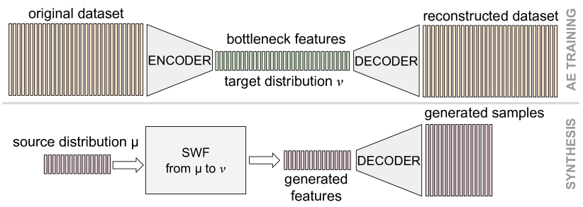
Figure 2: First, we learn an autoencoder (AE). Then, we use SWF to transport random vectors to the distribution of the bottleneck features of the training set. The trained decoder is used for visualization.

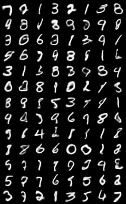
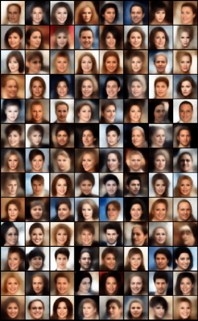
Figure 3: Samples generated after 200 iterations of SWF to match the distribution of bottleneck features for the training dataset. Visualization is done with the pre-trained decoder.

In the second set of experiments, we test the SWF algorithm on two real datasets. (i) The traditional MNIST dataset that contains 70K binary images corresponding to different digits. (ii) The popular CelebA dataset (Liu et al., 2015), that contains $202$K color-scale images. This dataset is advocated as more challenging than MNIST. Images were interpolated as $32\times 32$ for MNIST, and $64\times 64$ for CelebA.

In experiments reported in the supplementary document, we found out that directly applying SWF to such high-dimensional data yielded noisy results, possibly due to the insufficient sampling of $\mathbb{S}^{d-1}$. To reduce the dimensionality, we trained a standard convolutional autoencoder (AE) on the training set of both datasets (see Figure 2 and the supplementary document), and the target distribution $\nu$ considered becomes the distribution of the resulting bottleneck features, with dimension $d$. Particles can be visualized with the pre-trained decoder. Our goal is to show that SWF permits to directly sample from the distribution of bottleneck features, as an alternative to enforcing this distribution to match some prior, as in VAE. In the following, we set $\lambda=0$, $N_{\theta}=40000$, $d=32$ for MNIST and $d=64$ for CelebA.

Assessing the validity of IGM algorithms is generally done by visualizing the generated samples. Figure 3 shows some particles after $500$ iterations of SWF. We can observe they are considerably accurate. Interestingly, the generated samples gradually take the form of either digits or faces along the iterations, as seen on Figure 4. In this figure, we also display the closest sample from the original database to check we are not just reproducing training data.

Figure 4: Initial random particles (left), particles through iterations (middle, from 1 to 200 iterations) and closest sample from the training dataset (right), for both MNIST and CelebA.

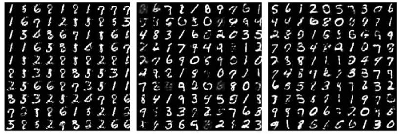
Figure 5: Performance of GAN (left), W-GAN (middle), SWG (right) on MNIST. (The figure is directly taken from (Deshpande et al., 2018).)

For a visual comparison, we provide the results presented in (Deshpande et al., 2018) in Figure 5. These results are obtained by running different IGM approaches on the MNIST dataset, namely GAN (Goodfellow et al., 2014), Wasserstein GAN (W-GAN) (Arjovsky et al., 2017) and the Sliced-Wasserstein Generator (SWG) (Deshpande et al., 2018). The visual comparison suggests that the samples generated by SWF are of slightly better quality than those, although research must still be undertaken to scale up to high dimensions without an AE.

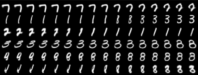
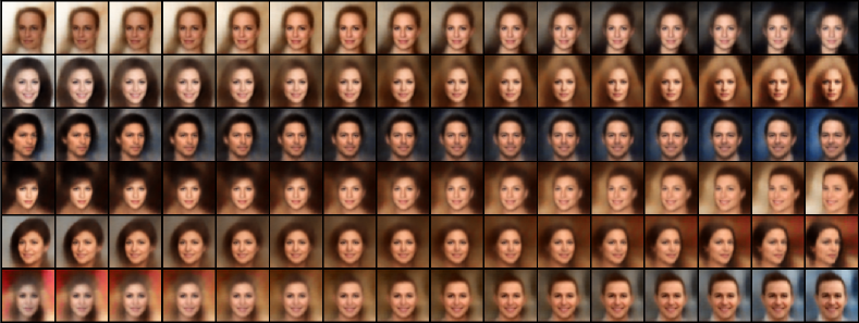
Figure 6: Applying a pre-trained SWF on new samples located in-between the ones used for training. Visualization is done with the pre-trained decoder.

We also provide the outcome of the pre-trained SWF with samples that are regularly spaced in between those used for training. The result is shown in Figure 6. This plot suggests that SWF is a way to interpolate non-parametrically in between latent spaces of regular AE.

5 Conclusion and Future Directions

In this study, we proposed SWF, an efficient, nonparametric IGM algorithm. SWF is based on formulating IGM as a functional optimization problem in Wasserstein spaces, where the aim is to find a probability measure that is close to the data distribution as much as possible while maintaining the expressiveness at a certain level. SWF lies in the intersection of OT, gradient flows, and SDEs, which allowed us to convert the IGM problem to an SDE simulation problem. We provided finite-time bounds for the infinite-particle regime and established explicit links between the algorithm parameters and the overall error. We conducted several experiments, where we showed that the results support our theory: SWF is able to generate samples from non-trivial distributions with low computational requirements.

The SWF algorithm opens up interesting future directions: (i) extension to differentially private settings (Dwork & Roth, 2014) by exploiting the fact that it only requires random projections of the data, (ii) showing the convergence scheme of the particle system (9) to the original SDE (8), (iii) providing bounds directly for the particle scheme (10).

1 Proof of Theorem 2

We first need to generalize (Bonnotte, 2013)[Lemma 5.4.3] to distribution $\rho\in\mathrm{L}^{\infty}(\operatorname{\overline{B}}(0,r))$, $r>0$.

Theorem S4.

Let $\nu$ be a probability measure on $\operatorname{\overline{B}}(0,1)$ with a strictly positive smooth density. Fix a time step $h>0$, regularization constant $\lambda>0$ and a radius $r>\sqrt{d}$. For any probability measure $\mu_{0}$ on $\operatorname{\overline{B}}(0,r)$ with density $\rho_{0}\in\mathrm{L}^{\infty}(\operatorname{\overline{B}}(0,r))$, there is a probability measure $\mu$ on $\operatorname{\overline{B}}(0,r)$ minimizing:

$$\mathcal{G}(\mu)=\mathcal{F}^{\nu}_{\lambda}(\mu)+\frac{1}{2h}{\cal W}_{2}^{2}(\mu,\mu_{0}),$$

where $\mathcal{F}^{\nu}_{\lambda}$ is given by (5). Moreover the optimal $\mu$ has a density $\rho$ on $\operatorname{\overline{B}}(0,r)$ and:

$$||\rho||_{\mathrm{L}^{\infty}}\leq(1+h/\sqrt{d})^{d}||\rho_{0}||_{\mathrm{L}^{\infty}}.$$ (S1)

Proof.

The set of measures supported on $\operatorname{\overline{B}}(0,r)$ is compact in the topology given by ${\cal W}_{2}$ metric. Furthermore by (Ambrosio et al., 2008)[Lemma 9.4.3] ${\cal H}$ is lower semicontinuous on $({\cal P}(\operatorname{\overline{B}}(0,r)),{\cal W}_{2})$. Since by (Bonnotte, 2013)[Proposition 5.1.2, Proposition 5.1.3], ${\cal S}{\cal W}_{2}$ is a distance on ${\cal P}(\operatorname{\overline{B}}(0,r))$, dominated by $d^{-1/2}{\cal W}_{2}$, we have:

$$|{\cal S}{\cal W}_{2}(\pi_{0},\nu)-{\cal S}{\cal W}_{2}(\pi_{1},\nu)|\leq{\cal S}{\cal W}_{2}(\pi_{0},\pi_{1})\leq\frac{1}{\sqrt{d}}{\cal W}_{2}(\pi_{0},\pi_{1}).$$

The above means that ${\cal S}{\cal W}_{2}(\cdot,\nu)$ is continuous with respect to topology given by ${\cal W}_{2}$, which implies that ${\cal S}{\cal W}_{2}^{2}(\cdot,\nu)$ is continuous in this topology as well. Therefore $\mathcal{G}:{\cal P}(\operatorname{\overline{B}}(0,r))\to\left(-\infty,+\infty\right]$ is a lower semicontinuous function on the compact set $({\cal P}(\operatorname{\overline{B}}(0,r)),{\cal W}_{2})$. Hence there exists a minimum $\mu$ of $\mathcal{G}$ on $\mathcal{P}(\operatorname{\overline{B}}(0,r))$. Furthermore, since $\mathcal{H}(\pi)=+\infty$ for measures $\pi$ that do not admit a density with respect to Lebesgue measure, the measure $\mu$ must admit a density $\rho$.

If $\rho_{0}$ is smooth and positive on $\operatorname{\overline{B}}(0,r)$, the inequality S1 is true by (Bonnotte, 2013)[Lemma 5.4.3.] When $\rho_{0}$ is just in $\mathrm{L}^{\infty}(\operatorname{\overline{B}}(0,r))$, we proceed by smoothing. For $t\in(0,1]$, let $\rho_{t}$ be a function obtained by convolution of $\rho_{0}$ with a Gaussian kernel $(t,x,y)\mapsto(2\pi)^{d/2}\exp(\left\|x-y\right\|^{2}/2)$, restricting the result to $\operatorname{\overline{B}}(0,r)$ and normalizing to obtain a probability density. Then $(\rho_{t})_{t}$ are smooth positive densities, and it is easy to see that $\lim_{t\rightarrow 0}||\rho_{t}||_{\mathrm{L}^{\infty}}\leq||\rho_{0}||_{\mathrm{L}^{\infty}}$. Furthermore, if we denote by $\mu_{t}$ the measure on $\operatorname{\overline{B}}(0,r)$ with density $\rho_{t}$, then $\mu_{t}$ converge weakly to $\mu_{0}$. For $t\in(0,1]$ let $\hat{\mu}_{t}$ be the minimum of $\mathcal{F}^{\nu}_{\lambda}(\cdot)+\frac{1}{2h}{\cal W}_{2}^{2}(\cdot,\mu_{t})$, and let $\hat{\rho}_{t}$ be the density of $\hat{\mu}_{t}$. Using (Bonnotte, 2013)[Lemma 5.4.3.] we get

$$||\hat{\rho}_{t}||_{\mathrm{L}^{\infty}}\leq(1+h\sqrt{d})^{d}||\rho_{t}||_{\mathrm{L}^{\infty}}.$$

so $\hat{\rho_{t}}$ lies in a ball of finite radius in $\mathrm{L}^{\infty}$. Using compactness of $\mathcal{P}(\operatorname{\overline{B}}(0,r))$ in weak topology and compactness of closed ball in $\mathrm{L}^{\infty}(\operatorname{\overline{B}}(0,r))$ in weak star topology, we can choose a subsequence $\hat{\mu}_{t_{k}},\hat{\rho}_{t_{k}}$, $\lim_{k\to+\infty}t_{k}=0$, that converges along that subsequence to limits $\hat{\mu}$, $\hat{\rho}$. Obviously $\hat{\rho}$ is the density of $\hat{\mu}$, since for any continuous function $f$ on $\operatorname{\overline{B}}(0,r)$ we have:

$$\int\hat{\rho}fdx=\lim_{k\rightarrow\infty}\int\rho_{t_{k}}fdx=\lim_{k\rightarrow\infty}\int fd\mu_{t_{k}}=\int fd\mu.$$

Furthermore, since $\hat{\rho}$ is the weak star limit of a bounded subsequence, we have:

$$||\hat{\rho}||_{\mathrm{L}^{\infty}}\leq\limsup_{k\rightarrow\infty}(1+h\sqrt{d})^{d}||\rho_{t_{k}}||_{\mathrm{L}^{\infty}}\leq(1+h\sqrt{d})^{d}||\rho_{0}||_{\mathrm{L}^{\infty}}.$$

To finish, we just need to prove that $\hat{\mu}$ is a minimum of $\mathcal{G}$. We remind our reader, that we already established existence of some minimum $\mu$ (that might be different from $\hat{\mu}$). Since $\hat{\mu}_{t_{k}}$ converges weakly to $\hat{\mu}$ in $\mathcal{P}(\operatorname{\overline{B}}(0,r))$, it implies convergence in ${\cal W}_{2}$ as well since $\operatorname{\overline{B}}(0,r)$ is compact. Similarly $\mu_{t_{k}}$ converges to $\mu_{0}$ in ${\cal W}_{2}$. Using the lower semicontinuity of $\mathcal{G}$ we now have:

$$\mathcal{F}^{\nu}_{\lambda}(\hat{\mu})+\frac{1}{2h}{\cal W}_{2}^{2}(\hat{\mu},\mu_{0}) \leq\liminf_{k\rightarrow\infty}\left(\mathcal{F}^{\nu}_{\lambda}(\hat{\mu}_{t_{k}})+\frac{1}{2h}{\cal W}_{2}^{2}(\hat{\mu}_{t_{k}},\mu_{0})\right)$$

$$\leq\liminf_{k\rightarrow\infty}\mathcal{F}^{\nu}_{\lambda}(\mu)+\frac{1}{2h}{\cal W}_{2}^{2}(\mu,\mu_{t_{k}})$$

$$+\frac{1}{2h}{\cal W}_{2}^{2}(\hat{\mu}_{t_{k}},\mu_{0})-\frac{1}{2h}{\cal W}_{2}^{2}(\hat{\mu}_{t_{k}},\mu_{t_{k}})$$

$$=\mathcal{F}^{\nu}_{\lambda}(\mu)+\frac{1}{2h}{\cal W}_{2}^{2}(\mu,\mu_{0}),$$

where the second inequality comes from the fact, that $\hat{\mu}_{t_{k}}$ minimizes $\mathcal{F}^{\nu}_{\lambda}(\cdot)+\frac{1}{2h}{\cal W}_{2}^{2}(\cdot,\mu_{t_{k}})$. From the above inequality and previously established facts, it follows that $\hat{\mu}$ is a minimum of $\mathcal{G}$ with density satisfying S1. ∎

Definition 1.

Minimizing movement scheme Let $r>0$ and $\mathcal{F}:\mathbb{R_{+}}\times{\cal P}(\operatorname{\overline{B}}(0,r))\times{\cal P}(\operatorname{\overline{B}}(0,r))\rightarrow\mathbb{R}$ be a functional. Let $\mu_{0}\in{\cal P}(\operatorname{\overline{B}}(0,r))$ be a starting point. For $h>0$ a piecewise constant trajectory $\mu^{h}:[0,\infty)\rightarrow{\cal P}(\operatorname{\overline{B}}(0,r))$ for $\mathcal{F}$ starting at $\mu_{0}$ is a function such that:

• $\mu^{h}(0)=\mu_{0}$.

• $\mu^{h}$ is constant on each interval $[nh,(n+1)h)$, so $\mu^{h}(t)=\mu^{h}(nh)$ with $n=\lfloor t/h\rfloor$.

• $\mu^{h}((n+1)h)$ minimizes the functional $\zeta\mapsto\mathcal{F}(h,\zeta,\mu^{h}(nh))$, for all $n\in\mathbb{N}$.

We say $\hat{\mu}$ is a minimizing movement scheme for $\mathcal{F}$ starting at $\mu_{0}$, if there exists a family of piecewise constant trajectory $(\mu^{h})_{h>0}$ for $\mathcal{F}$ such that $\hat{\mu}$ is a pointwise limit of $\mu^{h}$ as $h$ goes to $0$, i.e. for all $t\in\mathbb{R}_{+}$, $\lim_{h\to 0}\mu^{h}(t)=\mu(t)$ in ${\cal P}(\operatorname{\overline{B}}(0,r))$. We say that $\tilde{\mu}$ is a generalized minimizing movement for $\mathcal{F}$ starting at $\mu_{0}$, if there exists a family of piecewise constant trajectory $(\mu^{h})_{h>0}$ for $\mathcal{F}$ and a sequence $(h_{n})_{n}$, $\lim_{n\to\infty}h_{n}=0$, such that $\mu^{h_{n}}$ converges pointwise to $\tilde{\mu}$.

Theorem S5.

Let $\nu$ be a probability measure on $\operatorname{\overline{B}}(0,1)$ with a strictly positive smooth density. Fix a regularization constant $\lambda>0$ and radius $r>\sqrt{d}$. Given an absolutely continuous measure $\mu_{0}\in\mathcal{P}(\operatorname{\overline{B}}(0,r))$ with density $\rho_{0}\in\mathrm{L}^{\infty}(\operatorname{\overline{B}}(0,r))$, there is a generalized minimizing movement scheme $(\mu_{t})_{t}$ in $\mathcal{P}(\operatorname{\overline{B}}(0,r))$ starting from $\mu_{0}$ for the functional defined by

$$\mathcal{F}^{\nu}(h,\mu_{+},\mu_{-})=\mathcal{F}^{\nu}_{\lambda}(\mu_{+})+\frac{1}{2h}{\cal W}_{2}^{2}(\mu_{+},\mu_{-}).$$ (S2)

Moreover for any time $t>0$, the probability measure $\mu_{t}=\mu(t)$ has density $\rho_{t}$ with respect to the Lebesgue measure and:

$$||\rho_{t}||_{\mathrm{L}^{\infty}}\leq e^{dt\sqrt{d}}||\rho_{0}||_{\mathrm{L}^{\infty}}.$$ (S3)

Proof.

We start by noting, that by S4 for any $h>0$ there exists a piecewise constant trajectory $\mu^{h}$ for S2 starting at $\mu_{0}$. Furthermore for $t\geq 0$ measure $\mu_{t}^{h}=\mu^{h}(t)$ has density $\rho_{t}^{h}$, and:

$$||\rho_{t}^{h}||_{\mathrm{L}^{\infty}}\leq e^{d\sqrt{d}(t+h)}||\rho_{0}||_{\mathrm{L}^{\infty}}.$$ (S4)

Let us choose $T>0$. We denote $\rho^{h}(t,x)=\rho_{t}^{h}(x)$. For $h\leq 1$, the functions $\rho^{h}$ lie in a ball in $\mathrm{L}^{\infty}([0,T]\times\operatorname{\overline{B}}(0,r))$, so from Banach-Alaoglu theorem there is a sequence $h_{n}$ converging to $0$, such that $\rho^{h_{n}}$ converges in weak-star topology in $\mathrm{L}^{\infty}([0,T]\times\operatorname{\overline{B}}(0,r))$ to a certain limit $\rho$. Since $\rho$ has to be nonnegative except for a set of measure zero, we assume $\rho$ is nonnegative. We denote $\rho_{t}(x)=\rho(t,x)$. We will prove that for almost all $t$, $\rho_{t}$ is a probability density and $\mu_{t}^{h_{n}}$ converges in ${\cal W}_{2}$ to a measure $\mu_{t}$ with density $\rho_{t}$.

First of all, for almost all $t\in[0,T]$, $\rho_{t}$ is a probability density, since for any Borel set $A\subseteq[0,T]$ the indicator of set $A\times\operatorname{\overline{B}}(0,r)$ is integrable, and hence by definition of the weak-star topology:

$$\int_{A}\int_{\operatorname{\overline{B}}(0,r)}\rho_{t}(x)dxdt=\lim_{n\rightarrow\infty}\int_{A}\int_{\operatorname{\overline{B}}(0,r)}\rho_{t}^{h_{n}}(x)dxdt,$$

and so we have to have $\int\rho_{t}(x)dx=1$ for almost all $t\in[0,T]$. Nonnegativity of $\rho_{t}$ follows from nonnegativity of $\rho$.

We will now prove, that for almost all $t\in[0,T]$ the measures $\mu_{t}^{h_{n}}$ converge to a measure with density $\rho_{t}$. Let $t\in(0,T)$, take $\delta<\min(T-t,t)$ and $\zeta\in\mathrm{C}^{1}(\operatorname{\overline{B}}(0,r))$. We have:

$$\left|\int_{\operatorname{\overline{B}}(0,r)}\zeta d\mu_{t}^{h_{n}}-\int_{\operatorname{\overline{B}}(0,r)}\zeta d\mu_{t}^{h_{m}}\right|\leq\\ \left|\int_{\operatorname{\overline{B}}(0,r)}\zeta d\mu_{t}^{h_{n}}-\frac{1}{2\delta}\int_{t-\delta}^{t+\delta}\int_{\operatorname{\overline{B}}(0,r)}\zeta d\mu_{s}^{h_{n}}ds\right|+\left|\int_{\operatorname{\overline{B}}(0,r)}\zeta d\mu_{t}^{h_{m}}-\frac{1}{2\delta}\int_{t-\delta}^{t+\delta}\int_{\operatorname{\overline{B}}(0,r)}\zeta d\mu_{s}^{h_{m}}ds\right|+\\ \left|\frac{1}{2\delta}\int_{t-\delta}^{t+\delta}\int_{\operatorname{\overline{B}}(0,r)}\zeta d\mu_{s}^{h_{m}}ds-\frac{1}{2\delta}\int_{t-\delta}^{t+\delta}\int_{\operatorname{\overline{B}}(0,r)}\zeta d\mu_{s}^{h_{n}}ds\right|.$$ (S5)

Because $\mu_{t}^{h_{n}}$ have densities $\rho_{t}^{h_{n}}$ and both $\rho^{h_{n}}$, $\rho^{h_{m}}$ converge to $\rho$ in weak-star topology, the last element of the sum on the right hand side converges to zero, as $n,m\rightarrow\infty$. Next, we get a bound on the other two terms.

First, if we denote by $\gamma$ the optimal transport plan between $\mu_{t}^{h_{n}}$ and $\mu_{s}^{h_{n}}$, we have:

$$\left|\int_{\operatorname{\overline{B}}(0,r)}\zeta d\mu_{t}^{h_{n}}-\int_{\operatorname{\overline{B}}(0,r)}\zeta d\mu_{s}^{h_{n}}\right|^{2}\leq\int_{\operatorname{\overline{B}}(0,r)\times\operatorname{\overline{B}}(0,r)}\left|\zeta(x)-\zeta(y)\right|^{2}d\gamma(x,y)\leq||\nabla\zeta||_{\infty}^{2}{\cal W}_{2}^{2}(\mu_{t}^{h_{n}},\mu_{s}^{h_{n}}).$$ (S6)

In addition, for $n_{t}=\lfloor t/h_{n}\rfloor$ and $n_{s}=\lfloor s/h_{n}\rfloor$ we have $\mu_{t}^{h_{n}}=\mu_{n_{t}h_{n}}^{h_{n}}$ and $\mu_{s}^{h_{n}}=\mu_{n_{s}h_{n}}^{h_{n}}$. For all $k\geq 0$ we have:

$${\cal W}_{2}^{2}(\mu_{kh_{n}}^{h_{n}},\mu_{(k+1)h_{n}}^{h_{n}})\leq 2h_{n}(\mathcal{F}^{\nu}_{\lambda}(\mu_{kh_{n}}^{h_{n}})-\mathcal{F}^{\nu}_{\lambda}(\mu_{(k+1)h_{n}}^{h_{n}}).$$ (S7)

Using this result and (S6) and assuming without loss of generality $n_{t}\leq n_{s}$, from the Cauchy-Schwartz inequality we get:

$${\cal W}_{2}^{2}(\mu_{t}^{h_{n}},\mu_{s}^{h_{n}}) \leq\left(\sum_{k=n_{t}}^{n_{s}-1}{\cal W}_{2}(\mu_{kh_{n}}^{h_{n}},\mu_{(k+1)h_{n}}^{h_{n}})\right)^{2}$$

$$\leq|n_{t}-n_{s}|\sum_{k=n_{t}}^{n_{s}1}{\cal W}_{2}^{2}(\mu_{kh_{n}}^{h_{n}},\mu_{(k+1)h_{n}}^{h_{n}})$$

$$\leq 2h_{n}|n_{t}-n_{s}|(\mathcal{F}^{\nu}_{\lambda}(\mu_{n_{t}h_{n}}^{h_{n}})-\mathcal{F}^{\nu}_{\lambda}(\mu_{n_{s}h_{n}}^{h_{n}}))\leq 2C(|t-s|+h_{n}),$$ (S8)

where we used for the last inequality, denoting $C=\mathcal{F}^{\nu}_{\lambda}(\mu_{0})-\min_{{\cal P}(\operatorname{\overline{B}}(0,r))}\mathcal{F}^{\nu}_{\lambda}$, that $(\mathcal{F}^{\nu}_{\lambda}(\mu_{kh_{n}}^{h_{n}}))_{n}$ is non-increasing by (S7) and $\min_{{\cal P}(\operatorname{\overline{B}}(0,r))}\mathcal{F}^{\nu}_{\lambda}$ is finite since $\mathcal{F}^{\nu}_{\lambda}$ is lower semi-continuous. Finally, using Jensen’s inequality, the above bound and S6 we get:

$$\left|\int_{\operatorname{\overline{B}}(0,r)}\zeta d\mu_{t}^{h_{n}}-\frac{1}{2\delta}\int_{t-\delta}^{t+\delta}\int_{\operatorname{\overline{B}}(0,r)}\zeta d\mu_{s}^{h_{n}}ds\right|^{2} \leq\frac{1}{2\delta}\int_{t-\delta}^{t+\delta}\left|\int_{\operatorname{\overline{B}}(0,r)}\zeta d\mu_{t}^{h_{n}}-\int_{\operatorname{\overline{B}}(0,r)}\zeta d\mu_{s}^{h_{n}}\right|^{2}ds$$

$$\leq\frac{C||\nabla\zeta||_{\infty}^{2}}{\delta}\int_{t-\delta}^{t+\delta}(|t-s|+h_{n})ds$$

$$\leq 2C||\nabla\zeta||_{\infty}^{2}(h_{n}+\delta).$$

Together with (S5), when taking $\delta=h_{n}$, this result means that $\int_{\operatorname{\overline{B}}(0,r)}\zeta d\mu_{t}^{h_{n}}$ is a Cauchy sequence for all $t\in(0,T)$. On the other hand, since $\rho^{h_{n}}$ converges to $\rho$ in weak-star topology on $\mathrm{L}^{\infty}$, the limit of $\int_{\operatorname{\overline{B}}(0,r)}\zeta d\mu_{t}^{h_{n}}$ has to be $\int_{\operatorname{\overline{B}}(0,r)}\zeta(x)\rho_{t}(x)dx$ for almost all $t\in(0,T)$. This means that for almost all $t\in[0,T]$ sequence $\mu_{t}^{h_{n}}$ converges to a measure $\mu_{t}$ with density $\rho_{t}$.

Let $S\in[0,T]$ be the set of times such that for $t\in S$ sequence $\mu_{t}^{h_{n}}$ converges to $\mu_{t}$. As we established almost all points from $[0,T]$ belong to $S$. Let $t\in[0,T]\setminus S$. Then, there exists a sequence of times $t_{k}\in S$ converging to $t$, such that $\mu_{t_{k}}$ converge to some limit $\mu_{t}$. We have:

$${\cal W}_{2}(\mu_{t}^{h_{n}},\mu_{t})\leq{\cal W}_{2}(\mu_{t}^{h_{n}},\mu_{t_{k}}^{h_{n}})+{\cal W}_{2}(\mu_{t_{k}}^{h_{n}},\mu_{t_{k}})+{\cal W}_{2}(\mu_{t_{k}},\mu_{t}).$$

From which we have for all $k\geq 1$:

$$\limsup_{n\rightarrow\infty}{\cal W}_{2}(\mu_{t}^{h_{n}},\mu_{t})\leq{\cal W}_{2}(\mu_{t_{k}},\mu_{t})+\limsup_{n\rightarrow\infty}{\cal W}_{2}(\mu_{t}^{h_{n}},\mu_{t_{k}}^{h_{n}}),$$

and using (S8), we get $\mu_{t}^{h_{n}}\rightarrow\mu_{t}$. Furthermore, the measure $\mu_{t}$ has to have density, since $\rho_{t}^{h_{n}}$ lie in a ball in $\mathrm{L}^{\infty}(\operatorname{\overline{B}}(0,r))$, so we can choose a subsequence of $\rho_{t}^{h_{n}}$ converging in weak-star topology to a certain limit $\hat{\rho}_{t}$, which is the density of $\mu_{t}$.

We use now the diagonal argument to get convergence for all $t>0$. Let $(T_{k})_{k=1}^{\infty}$ be a sequence of times increasing to infinity. Let $h_{n}^{1}$ be a sequence converging to $0$, such that $\mu_{t}^{h_{n}^{1}}$ converge to $\mu_{t}$ for all $t\in[0,T_{1}]$. Using the same arguments as above, we can choose a subsequence $h_{n}^{2}$ of $h_{n}^{1}$, such that $\mu_{t}^{h_{n}^{2}}$ converges to a limit $\mu_{t}$ for all $t\in[0,T_{2}]$. Inductively, we construct subsequences $h_{n}^{k}$, and in the end take $h_{n}=h_{n}^{n}$. For this subsequence we have that $\mu_{t}^{h_{n}}$ converges to $\mu_{t}$ for all $t>0$, and $\mu_{t}$ has a density satisfying the bound from the statement of the theorem.

Finally, note that (S5) follows from (S4). ∎

Theorem S6.

Let $(\mu_{t})_{t\geq 0}$ be a generalized minimizing movement scheme given by Theorem S5 with initial distribution $\mu_{0}$ with density $\rho_{0}\in\mathrm{L}(\operatorname{\overline{B}}(0,r))$. We denote by $\rho_{t}$ the density of $\mu_{t}$ for all $t\geq 0$. Then $\rho_{t}$ satisfies the continuity equation:

$$\frac{\partial\rho_{t}}{\partial t}+\operatorname{div}(v_{t}\rho_{t})+\lambda\Delta\rho_{t}=0\,,\quad\quad\quad v_{t}(x)=-\int_{\mathbb{S}^{d-1}}\psi_{t,\theta}^{\prime}(\langle x,\theta\rangle)\theta d\theta,$$

in a weak sense, that is for all $\xi\in\mathrm{C}_{c}^{\infty}([0,\infty)\times\operatorname{\overline{B}}(0,r))$ we have:

$$\int_{0}^{\infty}\int_{\operatorname{\overline{B}}(0,r)}\left[\frac{\partial\xi}{\partial t}(t,x)-v_{t}\nabla\xi(t,x)-\lambda\Delta\xi(t,x)\right]\rho_{t}(x)dxdt=-\int_{\operatorname{\overline{B}}(0,r)}\xi(0,x)\rho_{0}(x)dx.$$

Proof.

Our proof is based on the proof of (Bonnotte, 2013)[Theorem 5.6.1]. We proceed in five steps.

1. Let $h_{n}\rightarrow 0$ be a sequence given by Theorem S5, such that $\mu_{t}^{h_{n}}$ converges to $\mu_{t}$ pointwise. Furthermore we know that $\mu^{h_{n}}$ have densities $\rho^{h_{n}}$ that converge to $\rho$ in $\mathrm{L}^{r}$, for $r\geq 1$, and in weak-star topology in $\mathrm{L}^{\infty}$. Let $\xi\in\mathrm{C}_{c}^{\infty}([0,\infty)\times\operatorname{\overline{B}}(0,r))$. We denote $\xi_{k}^{n}(x)=\xi(kh_{n},x)$. Using part $1$ of the proof of (Bonnotte, 2013)[Theorem 5.6.1], we obtain:

   $$\int_{\operatorname{\overline{B}}(0,r)}\xi(0,x)\rho_{0}(x)dx+\int_{0}^{\infty}\int_{\operatorname{\overline{B}}(0,r)}\frac{\partial\xi}{\partial t}(t,x)\rho_{t}(x)dxdt\\ =\lim_{n\rightarrow\infty}-h_{n}\sum_{k=1}^{\infty}\int_{\operatorname{\overline{B}}(0,r)}\xi_{k}^{n}(x)\frac{\rho_{kh_{n}}^{h_{n}}(x)-\rho_{(k-1)h_{n}}^{h_{n}}(x)}{h_{n}}dx.$$ (S9)

2. Again, this part is the same as part $2$ of the proof of (Bonnotte, 2013)[Theorem 5.6.1]. For any $\theta\in\mathbb{S}^{d-1}$ we denote by $\psi_{t,\theta}$ the unique Kantorovich potential from $\theta_{\#}^{*}\mu_{t}$ to $\theta_{\#}^{*}\nu$, and by $\psi_{t,\theta}^{h_{n}}$ the unique Kantorovich potential from $\theta_{\#}^{*}\mu_{t}^{h_{n}}$ to $\theta_{\#}^{*}\nu$. Then, by the same reasoning as part $2$ of the proof of (Bonnotte, 2013)[Theorem 5.6.1], we get:

   $$\int_{0}^{\infty}\int_{\operatorname{\overline{B}}(0,r)}\int_{\mathbb{S}^{d-1}}(\psi_{t,\theta})^{\prime}(\langle\theta,x\rangle)\langle\theta,\nabla\xi(x,t)\rangle d\theta d\mu_{t}(x)dt\\ =\lim_{n\rightarrow\infty}h_{n}\sum_{k=1}^{\infty}\int_{\operatorname{\overline{B}}(0,r)}\int_{\mathbb{S}^{d-1}}\psi_{kh_{n},\theta}^{h_{n}}(\theta^{*})\langle\theta,\nabla\xi_{k}^{n}\rangle d\theta d\mu_{kh_{n}}^{h_{n}}.$$ (S10)

3. Since $\xi$ is compactly supported and smooth, $\Delta\xi$ is Lipschitz, and so for any $t\geq 0$ if we take $k=\lfloor t/h_{n}\rfloor$ we get $|\Delta\xi_{k}^{n}(x)-\Delta\xi(t,x)|\leq Ch_{n}$ for some constant $C$. Let $T>0$ be such that $\xi(t,x)=0$ for $t>T$. We have:

   $$\left|\sum_{k=1}^{\infty}h_{n}\int_{\operatorname{\overline{B}}(0,r)}\Delta\xi_{k}^{n}(x)\rho_{kh_{n}}^{h_{n}}(x)dx-\int_{0}^{+\infty}\int_{\operatorname{\overline{B}}(0,r)}\Delta\xi(t,x)\rho_{t}^{h_{n}}(x)dxdt\right|\leq CTh_{n}.$$

   On the other hand, we know, that $\rho^{h_{n}}$ converges to $\rho$ in weak star topology on $\mathrm{L}^{\infty}([0,T]\times\operatorname{\overline{B}}(0,r))$, and $\Delta\xi$ is bounded, so:

   $$\lim_{n\to+\infty}\left|\int_{0}^{+\infty}\int_{\operatorname{\overline{B}}(0,r)}\Delta\xi(t,x)\rho_{t}^{h_{n}}(x)dxdt-\int_{0}^{+\infty}\int_{\operatorname{\overline{B}}(0,r)}\Delta\xi(t,x)\rho_{t}(x)dxdt\right|=0.$$

   Combining those two results give:

   $$\lim_{n\rightarrow\infty}h_{n}\sum_{k=1}^{\infty}\int_{\operatorname{\overline{B}}(0,r)}\Delta\xi_{k}^{n}(x)\rho_{kh_{n}}^{h_{n}}(x)dx=\int_{0}^{+\infty}\int_{\operatorname{\overline{B}}(0,r)}\Delta\xi(t,x)\rho_{t}(x)dxdt.$$ (S11)

4. Let $\phi_{k}^{h_{n}}$ denote the unique Kantorovich potential from $\mu_{kh_{n}}^{h_{n}}$ to $\mu_{(k-1)h_{n}}^{h_{n}}$. Using (Bonnotte, 2013)[Propositions 1.5.7 and 5.1.7], as well as (Jordan et al., 1998)[Equation (38)] with $\Psi=0$, and optimality of $\mu_{kh_{n}}^{h_{n}}$, we get:

   $$\frac{1}{h_{n}}\int_{\operatorname{\overline{B}}(0,r)}\langle\nabla\phi_{k}^{h_{n}}(x),\nabla\xi_{k}^{n}(x)\rangle d\mu_{kh_{n}}^{h_{n}}(x)-\int_{\operatorname{\overline{B}}(0,r)}\int_{\mathbb{S}^{d-1}}(\psi_{kh_{n}}^{h_{n}})^{\prime}(\theta^{*})\langle\theta,\nabla\xi_{k}^{n}(x)\rangle d\theta d\mu_{kh_{n}}^{h_{n}}(x)\\ -\lambda\int_{\operatorname{\overline{B}}(0,r)}\Delta\xi_{k}^{n}(x)d\mu_{kh_{n}}^{h_{n}}(x),$$ (S12)

   which is the derivative of $\mathcal{F}^{\nu}_{\lambda}(\cdot)+\frac{1}{2h_{n}}{\cal W}_{2}^{2}(\cdot,\mu_{(k-1)h_{n}})$ in the direction given by vector field $\nabla\xi_{k}^{n}$ is zero.

   Let $\gamma$ be the optimal transport between $\mu_{kh_{n}}^{h_{n}}$ and $\mu_{(k-1)h_{n}}^{h_{n}}$. Then:

   $$\int_{\operatorname{\overline{B}}(0,r)}\xi_{k}^{n}(x)\frac{\rho_{kh_{n}}^{h_{n}}(x)-\rho_{(k-1)h_{n}}^{h_{n}}(x)}{h_{n}}dx=\frac{1}{h_{n}}\int_{\operatorname{\overline{B}}(0,r)}(\xi_{k}^{n}(y)-\xi_{k}^{n}(x))d\gamma(x,y).$$ (S13)

   $$\frac{1}{h_{n}}\int_{\operatorname{\overline{B}}(0,r)}\langle\nabla\phi_{k}^{h_{n}}(x),\nabla\xi_{k}^{n}(x)\rangle d\mu_{kh_{n}}^{h_{n}}(x)=\frac{1}{h_{n}}\int_{\operatorname{\overline{B}}(0,r)}\langle\nabla\xi_{k}^{n}(x),y-x\rangle d\gamma(x,y).$$ (S14)

   Since $\xi$ is $\mathrm{C}_{c}^{\infty}$, it has Lipschitz gradient. Let $C$ be twice the Lipschitz constant of $\nabla\xi$. Then we have $|\xi(y)-\xi(x)-\langle\nabla\xi(x),y-x\rangle|\leq C|x-y|^{2}$, and hence:

   $$\int_{\operatorname{\overline{B}}(0,r)}|\xi_{k}^{n}(y)-\xi_{k}^{n}(x)-\langle\nabla\xi_{k}^{n}(x),y-x\rangle|d\gamma(x,y)\leq C{\cal W}_{2}^{2}(\mu_{(k-1)h_{n}}^{h_{n}},\mu_{kh_{n}}^{h_{n}}).$$ (S15)

   Combining (S13), (S14) and (S15), we get:

   $$\left|\sum_{k=1}^{\infty}h_{n}\int_{\operatorname{\overline{B}}(0,r)}\xi_{k}^{n}(x)\frac{\rho_{kh_{n}}^{h_{n}}-\rho_{(k-1)h_{n}}^{h_{n}}}{h_{n}}dx+\sum_{k=1}^{\infty}h_{n}\int_{\operatorname{\overline{B}}(0,r)}\langle\nabla\phi_{k}^{h_{n}},\nabla\xi_{k}^{n}\rangle d\mu_{kh_{n}}^{h_{n}}\right|\\ \leq C\sum_{k=1}^{\infty}{\cal W}_{2}^{2}(\mu_{(k-1)h_{n}}^{h_{n}},\mu_{kh_{n}}^{h_{n}}).$$ (S16)

   As some $\mathcal{F}^{\nu}_{\lambda}$ have a finite minimum on $\mathcal{P}(\operatorname{\overline{B}}(0,r))$, we have:

   $$\sum_{k=1}^{\infty}{\cal W}_{2}^{2}(\mu_{(k-1)h_{n}}^{h_{n}},\mu_{kh_{n}}^{h_{n}}) \leq 2h_{n}\sum_{k=1}^{\infty}\mathcal{F}^{\nu}_{\lambda}(\mu_{(k-1)h_{n}}^{h_{n}})-\mathcal{F}^{\nu}_{\lambda}(\mu_{kh_{n}}^{h_{n}})$$ (S17)

   $$\leq 2h_{n}\left(\mathcal{F}^{\nu}_{\lambda}(\mu_{0})-\min_{\mathcal{P}(\operatorname{\overline{B}}(0,r))}\mathcal{F}^{\nu}_{\lambda}\right).$$

   and so the sum on the right hand side of the equation goes to zero as $n$ goes to infinity.

   From (S16), (S17) and (S12) we conclude:

   $$\lim_{n\rightarrow\infty}-h_{n}\sum_{k=1}^{\infty}\xi_{k}^{n}(x)\frac{\rho_{kh_{n}}^{h_{n}}-\rho_{(k-1)h_{n}}^{h_{n}}}{h_{n}}dx=\\ \lim_{n\rightarrow\infty}\left(h_{n}\sum_{k=1}^{\infty}\int_{\operatorname{\overline{B}}(0,r)}\int_{\mathbb{S}^{d-1}}\psi_{kh_{n},\theta}^{h_{n}}(\theta^{*})\langle\theta,\nabla\xi_{k}^{n}\rangle d\theta d\mu_{kh_{n}}^{h_{n}}+h_{n}\sum_{k=1}^{\infty}\int_{\operatorname{\overline{B}}(0,r)}\Delta\xi_{k}^{n}(x)\rho_{kh_{n}}^{h_{n}}(x)dx\right),$$ (S18)

   where both limits exist, since the difference of left hand side and right hand side of the equation goes to zero, while the left hand side converges to a finite value by (S9).

5. Combining (S9), (S10), (S11) and (S18) we get the result.

∎

2 Proof of Theorem 3

Before proceeding to the proof, let us first define the following Euler-Maruyama scheme which will be useful for our analysis:

$$\hat{X}_{k+1}=\hat{X}_{k}+h\hat{v}(\hat{X}_{k},\mu_{kh})+\sqrt{2\lambda h}Z_{n+1},$$ (S19)

where $\mu_{t}$ denotes the probability distribution of $X_{t}$ with $(X_{t})_{t}$ being the solution of the original SDE (8). Now, consider the probability distribution of $\hat{X}_{k}$ as $\hat{\mu}_{kh}$. Starting from the discrete-time process $(\hat{X}_{k})_{k\in\mathbb{N}_{+}}$, we first define a continuous-time process $(Y_{t})_{t\geq 0}$ that linearly interpolates $(\hat{X}_{k})_{k\in\mathbb{N}_{+}}$, given as follows:

$$dY_{t}=\tilde{v}_{t}(Y)dt+\sqrt{2\lambda}dW_{t},$$ (S20)

where $\tilde{v}_{t}(Y)\triangleq-\sum_{k=0}^{\infty}\hat{v}_{kh}(Y_{kh})\mathds{1}_{[kh,(k+1)h)}(t)$ and $\mathds{1}$ denotes the indicator function. Similarly, we define a continuous-time process $(U_{t})_{t\geq 0}$ that linearly interpolates $(\bar{X}_{k})_{k\in\mathbb{N}_{+}}$, defined by (13), given as follows:

$$dU_{t}=\bar{v}_{t}(U)dt+\sqrt{2\lambda}dW_{t},$$ (S21)

where $\bar{v}_{t}(U)\triangleq-\sum_{k=0}^{\infty}\hat{v}(U_{kh},\bar{\mu}_{kh})\mathds{1}_{[kh,(k+1)h)}(t)$ and $\bar{\mu}_{kh}$ denotes the probability distribution of $\bar{X}_{k}$. Let us denote the distributions of $(X_{t})_{t\in[0,T]}$, $(Y_{t})_{t\in[0,T]}$ and $(U_{t})_{t\in\left[0,T\right]}$ as $\pi_{X}^{T}$, $\pi_{Y}^{T}$ and $\pi_{U}^{T}$ respectively with $T=Kh$.

We consider the following assumptions:

H S1.

For all $\lambda>0$, the SDE (8) has a unique strong solution denoted by $(X_{t})_{t\geq 0}$ for any starting point $x\in\mathbb{R}^{d}$.

H S2.

There exits $L<\infty$ such that

$$\|v_{t}(x)-v_{t^{\prime}}(x^{\prime})\|\leq L(\|x-x^{\prime}\|+|t-t^{\prime}|),$$ (S22)

where $v_{t}(x)=v(x,\mu_{t})$ and

$$\|\hat{v}(x,\mu)-\hat{v}(x^{\prime},\mu^{\prime})\|\leq L(\|x-x^{\prime}\|+\|\mu-\mu^{\prime}\|_{\textnormal{TV}}).$$ (S23)

H S3.

For all $t\geq 0$, $v_{t}$ is dissipative, i.e. for all $x\in\mathbb{R}^{d}$,

$$\langle x,v_{t}(x)\rangle\geq m\|x\|^{2}-b,$$ (S24)

for some $m,b>0$.

H S4.

The estimator of the drift satisfies the following conditions:  $\mathbb{E}[\hat{v}_{t}]=v_{t}$ for all $t\geq 0$, and for all $t\geq 0$, $x\in\mathbb{R}^{d}$,

$$\mathbb{E}[\|\hat{v}(x,\mu_{t})-v(x,\mu_{t})\|^{2}]\leq 2\delta(L^{2}\|x\|^{2}+B^{2}),$$ (S25)

for some $\delta\in(0,1)$.

H S5.

For all $t\geq 0$: $|\Psi_{t}(0)|\leq A$ and $\|v_{t}(0)\|\leq B$, for $A,B\geq 0$, where $\Psi_{t}=\int_{\mathbb{S}^{d-1}}\psi_{t}(\left\langle\theta,\cdot\right\rangle)d\theta$.

We start by upper-bounding $\|\hat{\mu}_{Kh}-\mu_{T}\|_{\textnormal{TV}}$.

Lemma S1.

Assume that the conditions H S2, S4, S3 and S5 hold. Then, the following bound holds:

$$\|\hat{\mu}_{Kh}-\mu_{T}\|_{\textnormal{TV}}^{2}\leq\|\pi^{T}_{Y}-\pi_{X}^{T}\|_{\textnormal{TV}}^{2}\leq\frac{L^{2}K}{4\lambda}\Bigl{(}\frac{C_{1}h^{3}}{3}+3\lambda dh^{2}\Bigr{)}+\frac{C_{2}\delta Kh}{8\lambda},$$ (S26)

where $C_{1}\triangleq 12(L^{2}C_{0}+B^{2})+1$, $C_{2}\triangleq 2(L^{2}C_{0}+B^{2})$, $C_{0}\triangleq C_{e}+2(1\vee\frac{1}{m})(b+2B^{2}+d\lambda)$, and $C_{e}$ denotes the entropy of $\mu_{0}$.

Proof.

We use the proof technique presented in (Dalalyan, 2017; Raginsky et al., 2017). It is easy to verify that for all $k\in\mathbb{N}_{+}$, we have $Y_{kh}=\hat{X}_{k}$.

By Girsanov’s theorem to express the Kullback-Leibler (KL) divergence between these two distributions, given as follows:

$$\textnormal{KL}(\pi_{X}^{T}||\pi_{Y}^{T}) =\frac{1}{4\lambda}\int_{0}^{Kh}\mathbb{E}[\|v_{t}(Y_{t})+\tilde{v}_{t}(Y)\|^{2}]\>dt$$ (S27)

$$=\frac{1}{4\lambda}\sum_{k=0}^{K-1}\int_{kh}^{(k+1)h}\mathbb{E}[\|v_{t}(Y_{t})+\tilde{v}_{t}(Y)\|^{2}]\>dt$$ (S28)

$$=\frac{1}{4\lambda}\sum_{k=0}^{K-1}\int_{kh}^{(k+1)h}\mathbb{E}[\|v_{t}(Y_{t})-\hat{v}_{kh}(Y_{kh})\|^{2}]\>dt.$$ (S29)

By using $v_{t}(Y_{t})-\hat{v}_{kh}(Y_{kh})=(v_{t}(Y_{t})-v_{kh}(Y_{kh}))+(v_{kh}(Y_{kh})-\hat{v}_{kh}(Y_{kh}))$, we obtain

$$\textnormal{KL}(\pi_{X}^{T}||\pi_{Y}^{T})\leq \frac{1}{2\lambda}\sum_{k=0}^{K-1}\int_{kh}^{(k+1)h}\mathbb{E}[\|v_{t}(Y_{t})-{v}_{kh}(Y_{kh})\|^{2}]\>dt$$

$$+\frac{1}{2\lambda}\sum_{k=0}^{K-1}\int_{kh}^{(k+1)h}\mathbb{E}[\|v_{kh}(Y_{kh})-\hat{v}_{kh}(Y_{kh})\|^{2}]\>dt$$ (S30)

$$\leq \frac{L^{2}}{\lambda}\sum_{k=0}^{K-1}\int_{kh}^{(k+1)h}\bigl{(}\mathbb{E}[\|Y_{t}-Y_{kh}\|^{2}]+(t-kh)^{2}\bigr{)}\>dt$$

$$+\frac{1}{2\lambda}\sum_{k=0}^{K-1}\int_{kh}^{(k+1)h}\mathbb{E}[\|v_{kh}(Y_{kh})-\hat{v}_{kh}(Y_{kh})\|^{2}]\>dt.$$ (S31)

The last inequality is due to the Lipschitz condition H S2.

Now, let us focus on the term $\mathbb{E}[\|Y_{t}-Y_{kh}\|^{2}]$. By using (S20), we obtain:

$$Y_{t}-Y_{kh}=-(t-kh)\hat{v}_{kh}(Y_{kh})+\sqrt{2\lambda(t-kh)}Z,$$ (S32)

where $Z$ denotes a standard normal random variable. By adding and subtracting the term $-(t-kh)v_{kh}(Y_{kh})$, we have:

$$Y_{t}-Y_{kh}=-(t-kh)v_{kh}(Y_{kh})+(t-kh)(v_{kh}(Y_{kh})-\hat{v}_{kh}(Y_{kh}))+\sqrt{2\lambda(t-kh)}Z.$$ (S33)

Taking the square and then the expectation of both sides yields:

$$\mathbb{E}[\|Y_{t}-Y_{kh}\|^{2}]\leq 3(t-kh)^{2}\mathbb{E}[\|v_{kh}(Y_{kh})\|^{2}]+3(t-kh)^{2}\mathbb{E}[\|v_{kh}(Y_{kh})-\hat{v}_{kh}(Y_{kh})\|^{2}]$$

$$+6\lambda(t-kh)d.$$ (S34)

As a consequence of H S2 and H S5, we have $\|v_{t}(x)\|\leq L\|x\|+B$ for all $t\geq 0$, $x\in\mathbb{R}^{d}$. Combining this inequality with H S4, we obtain:

$$\mathbb{E}[\|Y_{t}-Y_{kh}\|^{2}]\leq 6(t-kh)^{2}(L^{2}\mathbb{E}[\|Y_{kh}\|^{2}]+B^{2})+6(t-kh)^{2}(L^{2}\mathbb{E}[\|Y_{kh}\|^{2}]+B^{2})$$

$$+6\lambda(t-kh)d$$ (S35)

$$= 12(t-kh)^{2}(L^{2}\mathbb{E}[\|Y_{kh}\|^{2}]+B^{2})+6\lambda(t-kh)d.$$ (S36)

By Lemma 3.2 of (Raginsky et al., 2017), we have $\mathbb{E}[\|Y_{kh}\|^{2}]\leq C_{0}\triangleq C_{e}+2(1\vee\frac{1}{m})(b+2B^{2}+d\lambda)$, where $C_{e}$ denotes the entropy of $\mu_{0}$. Using this result in the above equation yields:

$$\mathbb{E}[\|Y_{t}-Y_{kh}\|^{2}]\leq 12(t-kh)^{2}(L^{2}C_{0}+B^{2})+6\lambda(t-kh)d.$$ (S37)

We now focus on the term $\mathbb{E}[\|v_{kh}(Y_{kh})-\hat{v}_{kh}(Y_{kh})\|^{2}]$ in (S31). Similarly to the previous term, we can upper-bound this term as follows:

$$\mathbb{E}[\|v_{kh}(Y_{kh})-\hat{v}_{kh}(Y_{kh})\|^{2}]\leq 2\delta(L^{2}\mathbb{E}[\|Y_{kh}\|^{2}]+B^{2})$$ (S38)

$$\leq 2\delta(L^{2}C_{0}+B^{2}).$$ (S39)

By using (S37) and (S39) in (S31), we obtain:

$$\textnormal{KL}(\pi_{X}^{T}||\pi_{Y}^{T})\leq \frac{L^{2}}{\lambda}\sum_{k=0}^{K-1}\int_{kh}^{(k+1)h}\bigl{(}12(t-kh)^{2}(L^{2}C_{0}+B^{2})+6\lambda(t-kh)d+(t-kh)^{2}\bigr{)}dt$$

$$+\frac{1}{2\lambda}\sum_{k=0}^{K-1}\int_{kh}^{(k+1)h}2\delta(L^{2}C_{0}+B^{2})\>dt$$ (S40)

$$= \frac{L^{2}K}{\lambda}\Bigl{(}\frac{C_{1}h^{3}}{3}+\frac{6\lambda dh^{2}}{2}\Bigr{)}+\frac{C_{2}\delta Kh}{2\lambda},$$ (S41)

where $C_{1}=12(L^{2}C_{0}+B^{2})+1$ and $C_{2}=2(L^{2}C_{0}+B^{2})$.

Finally, by using the data processing and Pinsker inequalities, we obtain:

$$\|\hat{\mu}_{Kh}-\mu_{T}\|_{\textnormal{TV}}^{2}\leq\|\pi_{X}^{T}-\pi_{Y}^{T}\|_{\textnormal{TV}}^{2}\leq \frac{1}{4}\textnormal{KL}(\pi_{X}^{T}||\pi_{Y}^{T})$$ (S42)

$$= \frac{L^{2}K}{4\lambda}\Bigl{(}\frac{C_{1}h^{3}}{3}+3\lambda dh^{2}\Bigr{)}+\frac{C_{2}\delta Kh}{8\lambda}.$$ (S43)

This concludes the proof. ∎

Now, we bound the term $\|\bar{\mu}_{Kh}-\hat{\mu}_{Kh}\|_{\textnormal{TV}}$.

Lemma S2.

Assume that H S2 holds. Then the following bound holds:

$$\|\pi_{U}^{T}-\pi_{Y}^{T}\|_{\textnormal{TV}}^{2}\leq\frac{L^{2}Kh}{16\lambda}\|\pi_{X}^{T}-\pi_{U}^{T}\|_{\textnormal{TV}}^{2}.$$ (S44)

Proof.

We use that same approach than in Lemma S1. By Girsanov’s theorem once again, we have

$$\textnormal{KL}(\pi_{Y}^{T}||\pi_{U}^{T}) =\frac{1}{4\lambda}\sum_{k=0}^{K-1}\int_{kh}^{(k+1)h}\mathbb{E}[\|\hat{v}(U_{kh},\mu_{kh})-\hat{v}(U_{kh},\bar{\mu}_{kh})\|^{2}]\>dt,$$ (S45)

where $\pi_{U}^{T}$ denotes the distributions of $(U_{t})_{t\in[0,T]}$ with $T=Kh$. By using H S2, we have:

$$\textnormal{KL}(\pi_{Y}^{T}||\pi_{U}^{T}) \leq\frac{L^{2}h}{4\lambda}\sum_{k=0}^{K-1}\|\mu_{kh}-\bar{\mu}_{kh}\|_{\textnormal{TV}}^{2}$$ (S46)

$$\leq\frac{L^{2}Kh}{4\lambda}\|\pi_{X}^{T}-\pi_{U}^{T}\|_{\textnormal{TV}}^{2}.$$ (S47)

By applying the data processing and Pinsker inequalities, we obtain the desired result. ∎

2.1 Proof of Theorem 3

Here, we precise the statement of Theorem 3.

Theorem S7.

Assume that the assumptions in Lemma S1 and Lemma S2 hold. Then for $\lambda>\frac{KL^{2}h}{8}$, the following bound holds:

$$\|\bar{\mu}_{Kh}-\mu_{T}\|_{\textnormal{TV}}^{2} \leq\delta_{\lambda}\Biggl{\{}\frac{L^{2}K}{2\lambda}\Bigl{(}\frac{C_{1}h^{3}}{3}+3\lambda dh^{2}\Bigr{)}+\frac{C_{2}\delta Kh}{4\lambda}\Biggr{\}},$$ (S48)

where $\delta_{\lambda}=(1-\frac{KL^{2}h}{8\lambda})^{-1}$.

Proof.

We have the following decomposition: (with $T=Kh$)

$$\|\pi_{X}^{T}-\pi_{U}^{T}\|_{\textnormal{TV}}^{2} \leq 2\|\pi_{X}^{T}-\pi_{Y}^{T}\|_{\textnormal{TV}}^{2}+2\|\pi_{Y}^{T}-\pi_{U}^{T}\|_{\textnormal{TV}}^{2}$$ (S49)

$$\leq\frac{L^{2}K}{2\lambda}\Bigl{(}\frac{C_{1}h^{3}}{3}+3\lambda dh^{2}\Bigr{)}+\frac{C_{2}\delta Kh}{4\lambda}+\frac{L^{2}Kh}{8\lambda}\|\pi_{X}^{T}-\pi_{U}^{T}\|_{\textnormal{TV}}^{2}$$ (S50)

$$\leq\Bigl{(}1-\frac{KL^{2}h}{8\lambda}\Bigr{)}^{-1}\Biggl{\{}\frac{L^{2}K}{2\lambda}\Bigl{(}\frac{C_{1}h^{3}}{3}+3\lambda dh^{2}\Bigr{)}+\frac{C_{2}\delta Kh}{4\lambda}\Biggr{\}}.$$ (S51)

The second line follows from Lemma S1 and Lemma S2. Last line follows from the assumption that $\lambda$ is large enough. This completes the proof. ∎

3 Proof of Corollary 1

Proof.

Considering the bound given in Theorem 3, the choice $h$ implies that

$$\frac{\delta_{\lambda}L^{2}K}{2\lambda}\Bigl{(}\frac{C_{1}h^{3}}{3}+3\lambda dh^{2}\Bigr{)}\leq\varepsilon^{2}.$$ (S52)

This finalizes the proof. ∎

4 Additional Experimental Results

4.1 The Sliced Wasserstein Flow

The whole code for the Sliced Wasserstein Flow was implemented in Python, for use with Pytorch. The code was written so as to run efficiently on GPU, and is available on the publicly available repository related to this paper.

In practice, the SWF involves relatively simple operations, the most important being:

• For each random $\theta\in\{\theta_{n}\}_{n=1\dots N_{\theta}}$, compute its inner product with all items from a dataset and obtain the empirical quantiles for these projections.

• At each step $k$ of the SWF, for each projection $z=\left<\theta,\bar{X}^{i}_{k}\right>$, apply two piece-wise linear functions, corresponding to the scalar optimal transport $\psi_{k,\theta}^{\prime}(z)$.

Even if such steps are conceptually simple, the quantile and required linear interpolation functions were not available on GPU for any framework we could figure out at the time of writing this paper. Hence, we implemented them ourselves for use with Pytorch, and the interested reader will find the details in the Github repository dedicated to this paper.

Given these operations, putting a SWF implementation together is straightforward. The code provided allows not only to apply it on any dataset, but also provides routines to have the computation of these sketches running in the background in a parallel manner.

4.2 The need for dimension reduction through autoencoders

In this study, we used an autoencoder trained on the dataset as a dimension reduction technique, so that the SWF is applied to transport particles in a latent space of dimension $d\approx 50$, instead of the original $d>1000$ of image data.

The curious reader may wonder why SWF is not applied directly to this original space, and what performances should be expected there. We have done this experiment, and we found out that SWF has much trouble rapidly converging to satisfying samples. In figure S1, we show the progressive evolution of particles undergoing SWF when the target is directly taken as the uncompressed dataset.

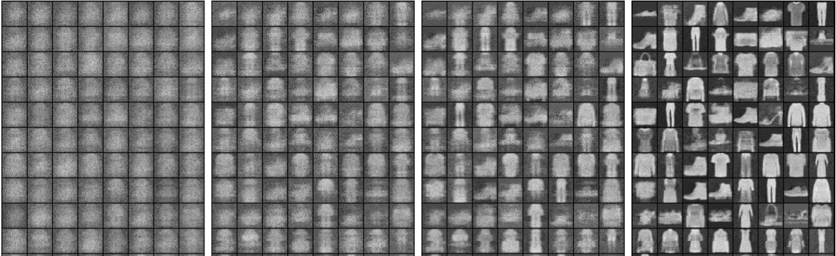
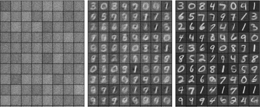
Figure S1: The evolution of SWF through 15000 iterations, when the original high-dimensional data is kept instead of working on reduced bottleneck features as done in the main document. Showing results on the MNIST and FashionMNIST datasets. For a visual comparison for FashionMNIST, we refer the reader to (Samangouei et al., 2018).

In this experiment, the strategy was to change the projections $\theta$ at each iteration, so that we ended up with a set of projections being $\{\theta_{n,k}\}_{n=1\dots N_{\theta}}^{k=1\dots K}$ instead of the fixed set of $N_{\theta}$ we now consider in the main document (for this, we picked $N_{\theta}=200$). This strategy is motivated by the complete failure we observed whenever we picked such fixed projections throughout iterations, even for a relatively large number as $N_{\theta}=16000$.

As may be seen on Figure S1, the particles definitely converge to samples from the desired datasets, and this is encouraging. However, we feel that the extreme number of iterations required to achieve such convergence comes from the fact that theory needs an integral over the $d-$dimensional sphere at each step of the SWF, which is clearly an issue whenever $d$ gets too large. Although our solution of picking new samples from the sphere at each iteration alleviated this issue to some extent, the curse of dimensionality prevents us from doing much better with just thousands of random projections at a time.

This being said, we are confident that good performance would be obtained if millions of random projections could be considered for transporting such high dimensional data because i/ theory suggests it and ii/ we observed excellent performance on reduced dimensions.

However, we, unfortunately, did not have the computing power it takes for such large scale experiments and this is what motivated us in the first place to introduce some dimension-reduction technique through AE.

4.3 Structure of our autoencoders for reducing data dimension

As mentioned in the text, we used autoencoders to reduce the dimensionality of the transport problem. The structure of these networks is the following:

• Encoder Four 2d convolution layers with (num_chan_out, kernel_size, stride, padding) being $(3,3,1,1)$, $(32,2,2,0)$, $(32,3,1,1)$, $(32,3,1,1)$, each one followed by a ReLU activation. At the output, a linear layer gets the desired bottleneck size.

• Decoder A linear layer gets from the bottleneck features to a vector of dimension $8192$, which is reshaped as $(32,16,16)$. Then, three convolution layers are applied, all with $32$ output channels and (kernel_size, stride, panning) being respectively $(3,1,1)$, $(3,1,1)$, $(2,2,0)$. A 2d convolution layer is then applied with an output number of channels being that of the data ($1$ for black and white, $3$ for color), and a (kernel_size, stride, panning) as $(3,1,1)$. In any case, all layers are followed by a ReLU activation, and a sigmoid activation is applied a the very output.

Once these networks defined, these autoencoders are trained in a very simple manner by minimizing the binary cross entropy between input and output over the training set of the considered dataset (here MNIST, CelebA or FashionMNIST). This training was achieved with the Adam algorithm (Kingma & Ba, 2014) with learning rate $1e-3$.

No additional training trick was involved as in Variational Autoencoder (Kingma & Welling, 2013) to make sure the distribution of the bottleneck features matches some prior. The core advantage of the proposed method in this respect is indeed to turn any previously learned AE as a generative model, by automatically and non-parametrically transporting particles drawn from an arbitrary prior distribution $\mu$ to the observed empirical distribution $\nu$ of the bottleneck features over the training set.

4.4 Convergence plots of SWF

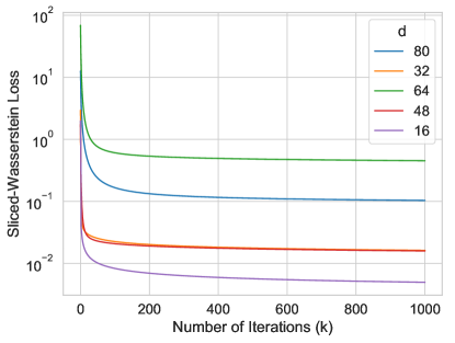
Figure S2: Approximately computed ${\cal S}{\cal W}_{2}$ between the output $\bar{\mu}_{k}^{N}$ and data distribution $\nu$ in the MNIST experiment for different dimensions $d$ for the bottleneck features (and the corresponding pre-trained AE).

In the same experimental setting as in the main document, we also illustrate the behavior of the algorithm for varying dimensionality $d$ for the bottleneck-features. To monitor the convergence of SWF as predicted by theory, we display the approximately computed ${\cal S}{\cal W}_{2}$ distance between the distribution of the particles and the data distribution. Even though minimizing this distance is not the real objective of our method, arguably, it is still a good proxy for understanding the convergence behavior.

Figure S2 illustrates the results. We observe that, for all choices of $d$, we see a steady and smooth decrease in the cost for all runs, which is in line with our theory. The absolute value of the cost for varying dimensions remains hard to interpret at this stage of our investigations.

5 Additional samples

5.1 Evolution throughout iterations

In Figures S3 and S4 below, we provide the evolution of the SWF algorithm on the Fashion MNIST and the MNIST datasets in higher resolution, for an AE with $d=48$ bottleneck features.

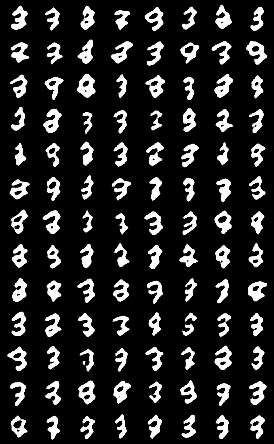
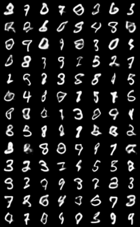
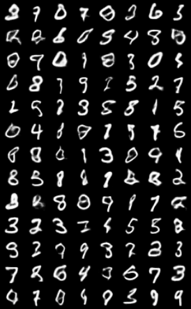
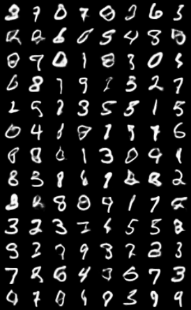
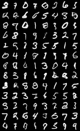
Figure S3: The evolution of SWF through 200 iterations on the MNIST dataset. Plots are for $1$, $11$, $21$, $31$, $41$, $51$, $101$ and $201$ iterations

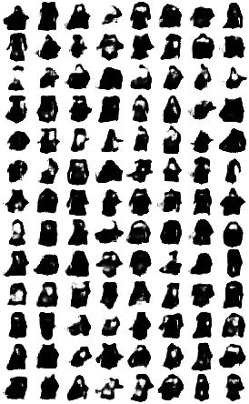
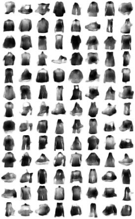
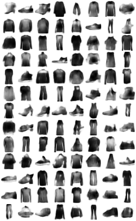
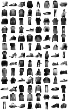
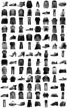
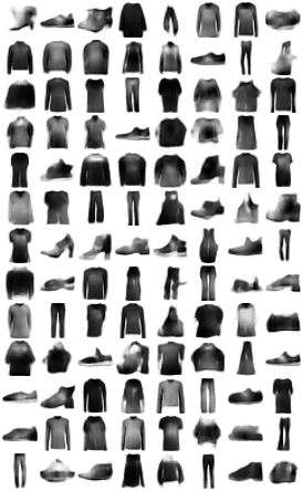
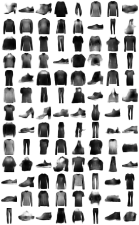
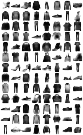
Figure S4: The evolution of SWF through 200 iterations on the FashionMNIST dataset. Plots are for $1$, $11$, $21$, $31$ (upper row) and $41$, $51$, $101$, $201$ (lower row) iterations

5.2 Training samples, interpolation and extrapolation

In Figures S5 and S6 below, we provide other examples of outcome from SWF, both for the MNIST and the FashionMNIST datasets, still with $d=48$ bottleneck features.

The most noticeable fact we may see on these figures is that while the actual particles which went through SWF, as well as linear combinations of them, all yield very satisfying results, this is however not the case for particles that are drawn randomly and then brought through a pre-learned SWF.

Once again, we interpret this fact through the curse of dimensionality: while we saw in our toy GMM example that using a pre-trained SWF was totally working for small dimensions, it is already not so for $d=48$ and only $3000$ training samples.

This noticed, we highlight that this generalization weakness of SWF for high dimensions is not really an issue, since it is always possible to i/ run SWF with more training samples if generalization is required ii/ re-run the algorithm for a set of new particles. Remember indeed that this does not require passing through the data again, since the distribution of the data projections needs to be done only once.

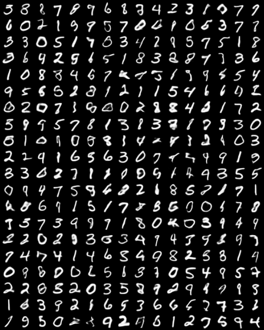
(a) particles undergoing SWF

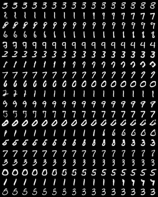
(b) After SWF is done: applying learned map on linear combinations of train particles

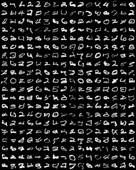
(c) After SWF is done: applying learned map on random inputs.

Figure S5: SWF on MNIST: training samples, interpolation in learned mapping, extrapolation.

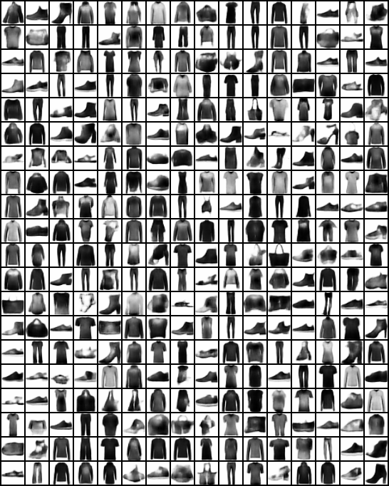
(a) particles undergoing SWF

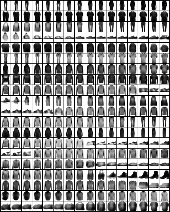
(b) After SWF is done: applying learned map on linear combinations of train particles

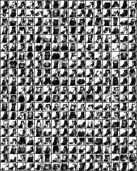
(c) After SWF is done: applying learned map on random inputs.

Figure S6: SWF on FashionMNIST: training samples, interpolation in learned mapping, extrapolation.

References

• Ambrosio et al. (2008) Ambrosio, L., Gigli, N., and Savaré, G. Gradient flows: in metric spaces and in the space of probability measures. Springer Science & Business Media, 2008.
• Arjovsky et al. (2017) Arjovsky, M., Chintala, S., and Bottou, L. Wasserstein generative adversarial networks. In International Conference on Machine Learning, pp. 214–223, 2017.
• Benamou & Brenier (2000) Benamou, J.-D. and Brenier, Y. A computational fluid mechanics solution to the Monge-Kantorovich mass transfer problem. Numerische Mathematik, 84(3):375–393, 2000.
• Bogachev et al. (2015) Bogachev, V. I., Krylov, N. V., Röckner, M., and Shaposhnikov, S. V. Fokker-Planck-Kolmogorov Equations, volume 207. American Mathematical Soc., 2015.
• Bonneel et al. (2015) Bonneel, N., Rabin, J., Peyré, G., and Pfister, H. Sliced and Radon Wasserstein barycenters of measures. Journal of Mathematical Imaging and Vision, 51(1):22–45, 2015.
• Bonnotte (2013) Bonnotte, N. Unidimensional and evolution methods for optimal transportation. PhD thesis, Paris 11, 2013.
• Bossy & Talay (1997) Bossy, M. and Talay, D. A stochastic particle method for the McKean-Vlasov and the Burgers equation. Mathematics of Computation of the American Mathematical Society, 66(217):157–192, 1997.
• Bousquet et al. (2017) Bousquet, O., Gelly, S., Tolstikhin, I., Simon-Gabriel, C.-J., and Schoelkopf, B. From optimal transport to generative modeling: the vegan cookbook. arXiv preprint arXiv:1705.07642, 2017.
• Cattiaux et al. (2008) Cattiaux, P., Guillin, A., and Malrieu, F. Probabilistic approach for granular media equations in the non uniformly convex case. Prob. Theor. Rel. Fields, 140(1-2):19–40, 2008.
• Şimşekli et al. (2018) Şimşekli, U., Yildiz, C., Nguyen, T. H., Cemgil, A. T., and Richard, G. Asynchronous stochastic quasi-Newton MCMC for non-convex optimization. In ICML, pp.  4674–4683, 2018.
• Cuturi (2013) Cuturi, M. Sinkhorn distances: Lightspeed computation of optimal transport. In Advances in neural information processing systems, pp. 2292–2300, 2013.
• Dalalyan (2017) Dalalyan, A. S. Theoretical guarantees for approximate sampling from smooth and log-concave densities. Journal of the Royal Statistical Society: Series B (Statistical Methodology), 79(3):651–676, 2017.
• Deshpande et al. (2018) Deshpande, I., Zhang, Z., and Schwing, A. Generative modeling using the sliced wasserstein distance. arXiv preprint arXiv:1803.11188, 2018.
• Diggle & Gratton (1984) Diggle, P. J. and Gratton, R. J. Monte carlo methods of inference for implicit statistical models. Journal of the Royal Statistical Society. Series B (Methodological), pp.  193–227, 1984.
• Donoho & Tanner (2009) Donoho, D. and Tanner, J. Observed universality of phase transitions in high-dimensional geometry, with implications for modern data analysis and signal processing. Philosophical Transactions of the Royal Society of London A: Mathematical, Physical and Engineering Sciences, 367(1906):4273–4293, 2009.
• Durmus et al. (2016) Durmus, A., Şimşekli, U., Moulines, E., Badeau, R., and Richard, G. Stochastic gradient Richardson-Romberg Markov Chain Monte Carlo. In NIPS, 2016.
• Dwork & Roth (2014) Dwork, C. and Roth, A. The algorithmic foundations of differential privacy. Foundations and Trends® in Theoretical Computer Science, 9(3–4):211–407, 2014.
• Genevay et al. (2016) Genevay, A., Cuturi, M., Peyré, G., and Bach, F. Stochastic optimization for large-scale optimal transport. In Advances in Neural Information Processing Systems, pp. 3440–3448, 2016.
• Genevay et al. (2017) Genevay, A., Peyré, G., and Cuturi, M. Gan and vae from an optimal transport point of view. arXiv preprint arXiv:1706.01807, 2017.
• Genevay et al. (2018) Genevay, A., Peyré, G., and Cuturi, M. Learning generative models with Sinkhorn divergences. In International Conference on Artificial Intelligence and Statistics, pp.  1608–1617, 2018.
• Goodfellow et al. (2014) Goodfellow, I., Pouget-Abadie, J., Mirza, M., Xu, B., Warde-Farley, D., Ozair, S., Courville, A., and Bengio, Y. Generative adversarial nets. In Advances in neural information processing systems, pp. 2672–2680, 2014.
• Gribonval et al. (2017) Gribonval, R., Blanchard, G., Keriven, N., and Traonmilin, Y. Compressive statistical learning with random feature moments. arXiv preprint arXiv:1706.07180, 2017.
• Gulrajani et al. (2017) Gulrajani, I., Ahmed, F., Arjovsky, M., Dumoulin, V., and Courville, A. C. Improved training of Wasserstein GANs. In Advances in Neural Information Processing Systems, pp. 5769–5779, 2017.
• Guo et al. (2017) Guo, X., Hong, J., Lin, T., and Yang, N. Relaxed Wasserstein with applications to GANs. arXiv preprint arXiv:1705.07164, 2017.
• Jordan et al. (1998) Jordan, R., Kinderlehrer, D., and Otto, F. The variational formulation of the Fokker–Planck equation. SIAM journal on mathematical analysis, 29(1):1–17, 1998.
• Kingma & Ba (2014) Kingma, D. and Ba, J. Adam: A method for stochastic optimization. arXiv preprint arXiv:1412.6980, 2014.
• Kingma & Welling (2013) Kingma, D. P. and Welling, M. Auto-encoding variational bayes. arXiv preprint arXiv:1312.6114, 2013.
• Kolouri et al. (2018) Kolouri, S., Martin, C. E., and Rohde, G. K. Sliced-wasserstein autoencoder: An embarrassingly simple generative model. arXiv preprint arXiv:1804.01947, 2018.
• Lavenant et al. (2018) Lavenant, H., Claici, S., Chien, E., and Solomon, J. Dynamical optimal transport on discrete surfaces. In SIGGRAPH Asia 2018 Technical Papers, pp.  250. ACM, 2018.
• Lei et al. (2017) Lei, N., Su, K., Cui, L., Yau, S.-T., and Gu, D. X. A geometric view of optimal transportation and generative model. arXiv preprint arXiv:1710.05488, 2017.
• Liu et al. (2017) Liu, S., Bousquet, O., and Chaudhuri, K. Approximation and convergence properties of generative adversarial learning. In Advances in Neural Information Processing Systems, pp. 5551–5559, 2017.
• Liu et al. (2015) Liu, Z., Luo, P., Wang, X., and Tang, X. Deep learning face attributes in the wild. In Proceedings of International Conference on Computer Vision (ICCV), 2015.
• Ma et al. (2015) Ma, Y. A., Chen, T., and Fox, E. A complete recipe for stochastic gradient MCMC. In Advances in Neural Information Processing Systems, pp. 2899–2907, 2015.
• Malrieu (2003) Malrieu, F. Convergence to equilibrium for granular media equations and their Euler schemes. Ann. Appl. Probab., 13(2):540–560, 2003.
• Mishura & Veretennikov (2016) Mishura, Y. S. and Veretennikov, A. Y. Existence and uniqueness theorems for solutions of McKean–Vlasov stochastic equations. arXiv preprint arXiv:1603.02212, 2016.
• Mohamed & Lakshminarayanan (2016) Mohamed, S. and Lakshminarayanan, B. Learning in implicit generative models. arXiv preprint arXiv:1610.03483, 2016.
• Nguyen et al. (2019) Nguyen, T. H., Şimşekli, U., , and Richard, G. Non-asymptotic analysis of fractional Langevin Monte Carlo for non-convex optimization. In ICML, 2019.
• Rabin et al. (2012) Rabin, J., Peyré, G., Delon, J., and Bernot, M. Wasserstein barycenter and its application to texture mixing. In Bruckstein, A. M., ter Haar Romeny, B. M., Bronstein, A. M., and Bronstein, M. M. (eds.), Scale Space and Variational Methods in Computer Vision, pp.  435–446, Berlin, Heidelberg, 2012. Springer Berlin Heidelberg. ISBN 978-3-642-24785-9.
• Raginsky et al. (2017) Raginsky, M., Rakhlin, A., and Telgarsky, M. Non-convex learning via stochastic gradient Langevin dynamics: a nonasymptotic analysis. In Proceedings of the 2017 Conference on Learning Theory, volume 65, pp.  1674–1703, 2017.
• Samangouei et al. (2018) Samangouei, P., Kabkab, M., and Chellappa, R. Defense-GAN: Protecting classifiers against adversarial attacks using generative models. In International Conference on Learning Representations, 2018.
• Santambrogio (2014) Santambrogio, F. Introduction to optimal transport theory. In Pajot, H., Ollivier, Y., and Villani, C. (eds.), Optimal Transportation: Theory and Applications, chapter 1. Cambridge University Press, 2014.
• Santambrogio (2017) Santambrogio, F. $\{$Euclidean, metric, and Wasserstein$\}$ gradient flows: an overview. Bulletin of Mathematical Sciences, 7(1):87–154, 2017.
• Şimşekli (2017) Şimşekli, U. Fractional Langevin Monte Carlo: Exploring Lévy Driven Stochastic Differential Equations for Markov Chain Monte Carlo. In International Conference on Machine Learning, 2017.
• Tolstikhin et al. (2017) Tolstikhin, I., Bousquet, O., Gelly, S., and Schoelkopf, B. Wasserstein auto-encoders. arXiv preprint arXiv:1711.01558, 2017.
• Van der Vaart (1998) Van der Vaart, A. W. Asymptotic statistics, volume 3. Cambridge university press, 1998.
• Veretennikov (2006) Veretennikov, A. Y. On ergodic measures for McKean-Vlasov stochastic equations. In Monte Carlo and Quasi-Monte Carlo Methods 2004, pp. 471–486. Springer, 2006.
• Villani (2008) Villani, C. Optimal transport: old and new, volume 338. Springer Science & Business Media, 2008.
• Welling & Teh (2011) Welling, M. and Teh, Y. W. Bayesian learning via stochastic gradient Langevin dynamics. In International Conference on Machine Learning, pp. 681–688, 2011.
• Wu et al. (2018) Wu, J., Huang, Z., Li, W., and Gool, L. V. Sliced wasserstein generative models. arXiv preprint arXiv:1706.02631, abs/1706.02631, 2018.
• Zhang et al. (2018) Zhang, J., Zhang, R., and Chen, C. Stochastic particle-optimization sampling and the non-asymptotic convergence theory. arXiv preprint arXiv:1809.01293, 2018.