Arbitrage–Free Interpolation in Models of Market Observable Interest Rates
Abstract.
Models which postulate lognormal dynamics for interest rates which are compounded according to market conventions, such as forward LIBOR or forward swap rates, can be constructed initially in a discrete tenor framework. Interpolating interest rates between maturities in the discrete tenor structure is equivalent to extending the model to continuous tenor. The present paper sets forth an alternative way of performing this extension; one which preserves the Markovian properties of the discrete tenor models and guarantees the positivity of all interpolated rates.
Practitioners have long priced caps, floors and other interest rate derivative contracts by Black/ Scholes–like111cf. ? (?). formulae, a practice usually attributed to the work of ? (?). Initially, this approach was very much focused on the pricing of individual contracts, without regard to the arbitrage relationships between different fixed income instruments. The seminal paper of ? (?) instigated further research into models of the entire yield curve and fitting initial data, where the yield curve was given either terms of zero coupon bond prices222cf. such papers as ? (?) or ? (?). or continuously compounded short or forward rates. The latter approach was taken by ? (?) (HJM), who developed a general framework for models of the term structure of interest rates, deriving drift conditions for instantaneous forward rates which must be satisfied in any arbitrage–free model. Thus the fundamental objects of these models were mainly mathematical constructs, not market observables. The first work to move away from this paradigm was ? (?, ?), who construct a binomial term structure model with the short rate compounded according to market conventions (e.g. three–month LIBOR) as the fundamental model variable. Taking the modelling of market observable interest rates to continuous time and bringing theoretical developments back into line with widespread market practice, ? (?)333See also ? (?) and ? (?). (MSS) embedded the pricing of caps and floors by Black/Scholes–like formulae in a consistent HJM framework. The critical assumption for this result is that relative volatility444The relative volatility of a diffusion process is if its quadratic variation is given by . of observable market forward rates such as LIBOR is deterministic.555For a succinct treatment of the significance of this assumption, see ? (?).
? (?) (BGM) resolved key questions in the construction of such a model, in particular concerning existence and measure relationships. Given the deterministic volatility assumption, they explicitly identified forward LIBOR as lognormal martingales under the forward measure to the end of the respective accrual periods. Their label Market Models seems to have become the generally accepted descriptor for models which postulate lognormality (under the appropriate probability measure) for market observable interest rates. The same methodology can be applied to forward swap rates to derive a model which supports the market practice of pricing swaptions by a Black/Scholes–type formula, as demonstrated by ? (?). ? (?) use a similar approach to construct a model of lognormal futures rates (implied by the prices of interest rate futures), which nests the lognormal forward LIBOR model.
Starting point of our discussion is the work of ? (?), who bring important clarity into the construction of lognormal market models. Besides explicitly deriving the relationships between forward measures of different maturities, they set up the model of lognormal forward LIBORs for a discrete set of maturities (the tenor structure) first and then extend it to a continuum of maturities by applying the assumptions of BGM, i.e. lognormality of all forward rates with compounding period and zero volatility for all zero coupon bonds with time to maturity less than . This makes transparent the fact that extending the model to continuous tenor in effect stipulates how the model will interpolate between a discrete set of maturities. Note that in all cases considered in the present paper the stochastic dynamics of interest rates are modelled in continuous time. Interpolation occurs in the maturity dimension only. Furthermore, the rates modelled have a fixed maturity (as opposed to a fixed time–to–maturity). In simple terms, the question addressed is how to determine the continuous time dynamics of, say, the yield for an investment maturing next August given the continuous time dynamics of three–month forward rates for accrual periods starting in March, June, September and December of every year.
Specifying lognormal dynamics for all –compounded forward rates, as MSS and BGM do, has the obvious advantage that all caplets and floorlets on such rates are valued by Black/Scholes–like formulae. However, this elegance comes at a price. For one, the no–arbitrage with cash property cannot be guaranteed, i.e. although the forward LIBORs modelled as lognormal will always be positive, other rates may not be.666? (?) give an example of this. Second, the Markovian properties of the discrete tenor model are lost; this is a fact which can cause considerable problems in numerical implementations, including Monte Carlo simulation, as we will discuss below. Third, one may take the pragmatic point of view that in reality one observes only a discrete number of rates on the market, with the rest determined by some interpolation method of choice. Thus one may prefer a version of the model which implies an interpolation method for future dates that is transparent and tractable. As the approach of ? (?) to the construction of a continuous tenor model makes clear, once volatilities are specified for continuous tenor, one has the freedom to arbitrarily interpolate initial observed market rates. Thereafter, interpolation is fixed by no arbitrage conditions and must be evaluated numerically.
The alternative way of extending a lognormal market model from discrete to continuous tenor proposed here addresses each of these points. It is also worthy to note that while the practical relevance of the lognormal market models makes the deterministic volatility case a natural focus of attention, Musiela and Rutkowski’s forward measure approach to term structure modelling is valid for much more general volatility specifications, and this generality carries over to a large part of the results presented here. In particular, this is true for other models constructed in discrete tenor, such as the lognormal forward swap rate model of ? (?).
In the present paper, the extension to continuous tenor is initially performed by deterministically interpolating zero coupon bond prices maturing before the earliest (future) date in the tenor structure (the “short bonds”), not only for the initial term structure, but at any future time as well (section 1). At any point in time, interpolation of longer–dated bonds is determined by no arbitrage conditions (section 2). Interpolating short bond prices from the two adjacent discrete tenor LIBORs introduces volatility for the short bonds and the associated interest rates (section 3). The dynamics of all interpolated rates remain Markovian in the state vector of discrete tenor forward LIBORs (section 4). The properties of the interpolated rates are discussed in section 5. Section 6 analyses the implications for the pricing of cap/floor contacts which do not fit into the discrete tenor structure and section 7 concludes.
1. Interpolation of Short–dated Bonds
Given a filtered probability space satisfying the usual conditions, let denote a –dimensional standard Wiener process and assume that the filtration is the usual –augmentation of the filtration generated by .
The model is set up on the basis of assumptions (BP.1) and (BP.2) of ? (?):
-
(BP.1)
For any date , the price process of a zero coupon bond , is a strictly positive special martingale under .
-
(BP.2)
For any fixed , the forward process
follows a martingale under .
Note that assumption (BP.2) means that can be interpreted as the time forward measure and implies that the bond price dynamics are arbitrage–free.
The objects to be modelled on the fixed income markets are the -compounded forward rates defined by
| (1) |
Since the compounding matches the market convention for rates such as the London Interbank Offer Rate, is also referred to as forward LIBOR.
Consider a discrete tenor structure . For notational simplicity, let also be the time origin and . The dynamics of the rates , , are given as in the discrete tenor version of the lognormal forward rate model put forth by ? (?):777Note that the focus here is on lognormal forward LIBOR models for expositional purposes only, because this represents the mainstream of the literature. The results presented here apply equally well to the discrete tenor versions of other models of market observable rates, such as the lognormal forward swap rate model of ? (?) or extensions such models to more general volatility functions, such as the model of level–dependent LIBOR volatilities proposed by ? (?).
| (2) |
where is a -dimensional standard Brownian motion under the time forward measure and is a deterministic function of its arguments, i.e. each is a lognormal martingale under .888For details of the model construction, see ? (?).
Define the function
as
Similarly to the extensions to continuous tenor proposed in ? (?) and ? (?), we initially make the following
1.1 Assumption.
Let volatility be zero for all zero coupon bonds maturing by the next (future) date in the tenor structure , i.e. .
Consequently, at time the price of the zero coupon bond maturing in is given by
and its dynamics are deterministic thereafter. Since they are deterministic, interpolation of interest rates with time to maturity less than is the same as specifying the evolution of the bond price, and arbitrary deterministic dynamics can be specified for , , with . For obvious reasons, these dynamics should be monotonically increasing and continuous, which means defining the continuously compounded short rate as some positive function999Note that this immediately implies that all interest rates generated by the model will be positive. , such that101010Given Assumption 1.1, (3) is simply a restatement of the identity (23) in ? (?).
| (3) |
Thus is an –measurable random variable. Consequently,
Note that while the dynamics of the abstract variable are in general discontinuous at each , any rate associated with a compounding period greater than length zero will have continuous dynamics.
1.2 Remark.
In a term structure model with zero volatility for zero coupon bonds for all , the risk neutral and rolling spot LIBOR measures are identical and the short rate interpolation (3) is arbitrage free.
Proof: The risk neutral equivalent martingale measure is conventionally defined as the measure associated with taking the (continuously compounded) savings account as the numeraire asset, i.e. under this measure all assets discounted by the savings account are martingales. The savings account defined by the interpolation is
| (4) | |||||
For the rolling spot LIBOR measure as introduced by ? (?), the numeraire is a roll–over strategy in which money is invested and subsequently reinvested at spot LIBOR. Investing one monetary unit in at the spot LIBOR is the same as buying zero coupon bonds , where . Thus in continuous tenor the value at time of the roll–over strategy is
| (5) |
Since is –measurable for , we have by construction that
for . Thus the numeraire processes are identical, which means that the associated martingale measures must be111111In a continuous tenor model, the market is (dynamically) complete, therefore the martingale measure for a given numeraire is unique. For an alternative proof, cf. Lemma 3.3 in ? (?)..
The interpolation defined by (3) is consistent with no arbitrage if the savings account given by (4) discounted by a numeraire asset is a martingale under the martingale measure associated with this numeraire. It is sufficient to verify this for one measure and by the above argument, this condition is trivially fulfilled since the value of the savings account is identically equal to the value of the spot LIBOR roll–over strategy.
In other words, since at any time the dynamics of the shortest remaining bond to a discrete tenor date are consistent with the deterministic interpolation for the continuously compounded short rate, all martingale properties (and thus no arbitrage) are preserved.
The observation that the roll–over strategy in spot LIBOR corresponds to a roll-over strategy in the shortest remaining bond to a discrete tenor date also leads us to the following
1.3 Remark.
Conditional on the information at time , for all –measurable events, the rolling spot LIBOR measure is identical to the forward measure of maturity , i.e.
Thus can be interpreted as “pasting together” a sequence of conditional forward measures. This is valid for any arbitrage free term structure model.
Proof: This is an immediate consequence of the fact that the time value of the spot LIBOR roll–over strategy (5) can be written, independently of how the discrete tenor model is extended to continuous tenor, as a –measurable factor times , the numeraire of the time forward measure.121212For a more formal statement of this proof, see ? (?).
2. Interpolation of Longer–dated Bonds
2.1 Remark.
Given a discrete tenor model and the interpolation of the short–dated zero coupon bonds , the continuous tenor model is completely specified.
Proof: Consider a completely arbitrary pair of time points , . The time price of a zero coupon bond maturing in is given by
| (6) |
where the short–dated bond is given by the interpolation and the bond price quotient on the far right by the no–arbitrage requirement that
Given a choice of interpolation (3), we can determine a function such that
| (7) |
In the lognormal case, the right hand side can easily be evaluated numerically and depends only on and deterministic volatilities.
When intermediate rates with LIBOR–type compounding are linearly interpolated by day–count fractions, (7) becomes very tractable for any model satisfying the assumptions (BP.1) and (BP.2). Define implicitly by setting
| (8) |
i.e.
Then
and
Note that by remark 2.1, if interpolation of short–dated bonds is specified for all times, there is no modelling freedom to interpolate longer–dated bonds, including initial model inputs. In addition to being intuitively appealing, linear interpolation by day–count fractions has the added attraction of providing one consistent interpolation method for all times and all maturities. Other popular interpolation methods, such as loglinear interpolation of discount factors or linear interpolation of continuously compounded yields, do not have this property.
3. Introducing Volatility for the Short Bonds
In some applications, setting short bond volatilities to zero may be unsatisfactory. Assumption 1.1 can certainly be relaxed in any way which satisfies the arbitrage constraints. Remark 2.1 remains valid, i.e. to extend the model to continuous tenor it is sufficient to specify the dynamics of the short bonds. However, when the short bond dynamics are stochastic, the constraint given by equation (3) is replaced by the more general formulation given in terms of instantaneous forward rates in equation (23) of ? (?):
| (9) |
where is the instantaneous forward rate at time for maturity .
One tractable and intuitively appealing way to introduce volatility for the interpolated short bonds is to make the interpolated rates dependent on the closest remaining forward LIBOR . Set
where
e.g.
As in section 2, the prices of bonds with longer maturities must satisfy
Using the expected value of under given in ? (?):
| (10) | |||||
The “correction factor” will usually be quite close to one, unless volatility is very high or time to maturity is very long. Thus interpolation remains essentially linear.
Note that since the short bonds are no longer deterministic, we also need to evaluate the appropriate expectation to derive for :
4. Forward Measures and the Markov Property
Both ? (?) and ? (?) set up the model of lognormal forward LIBORs in continuous tenor, i.e. equation (2) applies to all maturities :
with a deterministic function of its arguments, i.e. each is a lognormal martingale under for a continuum of maturities up to the time horizon . This has the advantage that all caps and floors on –compounded rates will be priced by the Black/Scholes–type formulae favoured by market practitioners.
The main disadvantage of this approach is revealed when one attempts to price instruments for which closed form solutions are unavailable. This is already the case if the cashflow underlying a derivative does not fit neatly into a tenor structure of –compounded rates and even more so for many popular interest rate exotics. The problem is that the continuous tenor model is infinite–dimensional even if the driving Brownian motion is one–dimensional. That is, the Markovian state variable for such a model is the entire yield curve.131313The term “yield curve” generally denotes the term structure interest rates for a continuum of maturities up to the time horizon. It can be represented in several equivalent ways, for example by the curve of all continuously compounded yields at time , with defined by This causes considerable difficulties for all types of numerical methods. Even the method of last resort for high–dimensional problems, Monte Carlo simulation, cannot handle infinite–dimensional state variables.
From the start, it has been part of the “folk wisdom” on these models that they do not permit a finite dimensional representation. ? (?) derive the dynamics of the continuously compounded short rate under a given set of assumptions on the volatility structure and show that they are highly path–dependent and thus not Markovian in any finite set of state variables. Recently, ? (?) formalised this conjecture and showed that when the model is driven by a one–dimensional Brownian motion, a finite–dimensional representation can only exist in the trivial case of zero volatility. He also derives similarly restrictive conditions on the finite–dimensional representability of continuous tenor LIBOR models driven by a multidimensional Brownian motion. These conditions, though stopping short of precluding finite–dimensional cases, indicate that such cases are not likely to be practically useful if they do exist.
The extensions of the discrete tenor model to continuous tenor proposed in the previous sections provide a way around this problem. Since the interpolated rates are specified as functions of the discrete tenor rates, the Markovian structure of the discrete tenor model is preserved. This structure can be characterised as follows:
4.1 Remark.
In the discrete tenor lognormal forward LIBOR model, consider the dynamics of a rate under some forward measure141414Note that the Markov property depends on the probability measure under consideration.. These dynamics are Markovian in a state variable vector consisting of rates with .
Proof: ? (?) show that the relationship between forward measures and is given by the Radon/Nikodym derivative
where is a Brownian motion under and
with the (deterministic) volatility of . Thus
Since the dynamics of are given by
the joint dynamics of all rates with under are
| (11) |
where
If is the dimension of the driving Brownian motion, is an matrix with
is an matrix with
Finally, is an –dimensional vector with
Conversely, under we have
| (12) |
with
By the Markov property of Ito diffusions, the dynamics given by (11) resp. (12) are Markov in .
This result does not rely on the assumption that the LIBOR volatilities are deterministic functions of their arguments. Rather, if the are level dependent on some or all rates in , the Markov property still holds. Also, by remark 1.3, the above result implies that under the rolling spot LIBOR measure, any rate is Markov in the state variable vector .
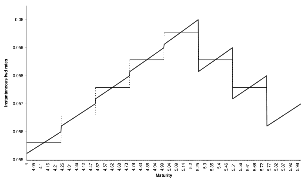
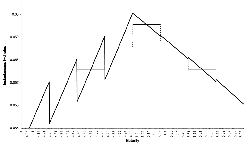
Interpolation by daycount fractions vs. interpolation with short bond volatility
5. A Look at the Interpolated Interest Rates
This section illustrates some of the properties of the interpolated interest rates and contrasts the two interpolation methods proposed in the previous sections. The method described in section 2 will be referred to as method 1 or interpolation by daycount fractions; the one introduced in section 3 will be labelled method 2 or interpolation with short bond volatility. For the inputs used to produce each of the plots, please refer to table 1 in the appendix. The algorithm from ? (?) was used to generate sample paths for the evolution of the term structure.
5.1. Term Structures
Figures 2 and 2 show how the two methods interpolate instantaneous forward rates. For reference, the stepwise constant rates resulting from loglinear interpolation of zero coupon bond prices are included in each plot. The instantaneous forward rates jump when one moves from one –compounding period to the next. From equations (8) and (9), this is to be expected, as the maturities of the LIBORs underlying the interpolation are different on each interval. Instantaneous forward rates on are determined on each interval by calculating
Instantaneous forward rates give the most disaggregate representation of the term structure and therefore effectively demonstrate the implications of the choice of interpolation method. However, one should not judge the usefulness of a particular method from this perspective alone. At first glance the “sawtooth” patterns of the interpolated rates for falling term structures in method 1 and rising term structures in method 2 seem to represent serious drawbacks to using either method, but one should keep in mind that the instantaneous forward rates are also purely mathematical artifacts, while the objects being modelled are market observable rates such as LIBOR. Forward LIBORs are interpolated by
| (13) | |||||
For method 1 this becomes
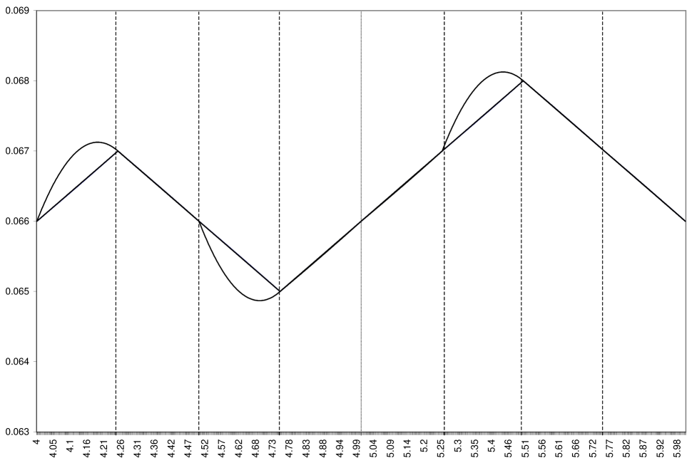
Figure 3 shows interpolated forward three–month LIBORs for a continuum of start dates between four and six years forward. The piecewise linear graph is actually two plots so close as to be indistinguishable: Interpolation by daycount fractions and loglinear interpolation of zero coupon bond prices results in nearly identical forward three–month LIBORs, even though the resulting instantaneous forward rates are very different. This also implies that if one is only concerned with rates such as forward three–month LIBORs, using loglinear interpolation of zero coupon bond prices is for all intents and purposes arbitrage free.
Introducing short bond volatility as per method 2 makes a difference for the interpolated LIBORs only when the interest rate term structure changes slope. The vertical gridlines in figure 3 represent boundaries between the accrual periods in the original discrete tenor. Interpolated forward LIBORs with start date in an accrual period immediately preceding a change in the slope of the term structure depart from the linearly interpolated plots and curve “outward”. This is due to the fact that a forward LIBOR for a given start date is interpolated using the forward LIBOR for the preceding and the two following discrete tenor start dates , and , as can easily be seen by appropriately inserting (10) into (13).
5.2. Rate Dynamics
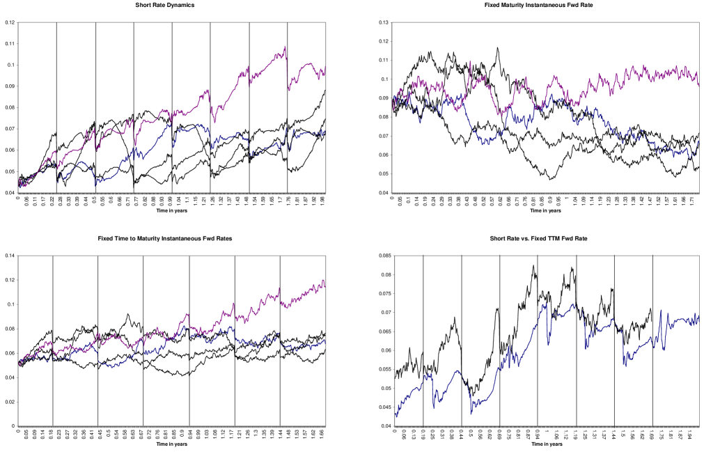
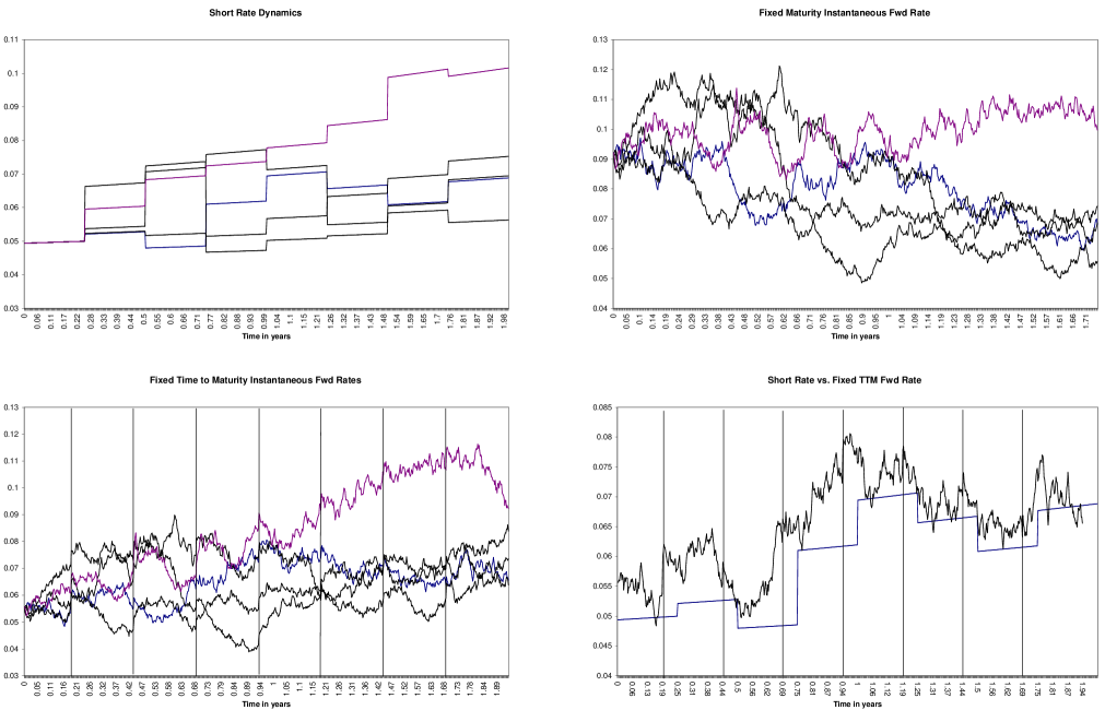
The dynamics which the two methods imply for interpolated rates are illustrated in Figures 4 and 5. Not only, as in the previous section, do equations (8) and (9) imply discontinuities in the instantaneous rates in the maturity dimension, but also in the time dimension. This becomes particularly clear in the dynamics of the continuously compounded short rate under interpolation by daycount fractions: This rate evolves deterministically within each accrual period of the discrete tenor structure and jumps at the accrual period boundaries. For instantaneous forward rates the dynamics are stochastic as long as the time to maturity is greater than the accrual period length . The maturity of the forward rate determines which forward LIBORs are used in the interpolation, so if one considers an instantaneous forward rate for a fixed maturity, this rate will be interpolated from the same forward LIBORs at all times. Since the LIBOR dynamics are modelled to be continuous, the interpolated rate will not jump (cf. plot in upper right of Figure 4). On the other hand, holding time to maturity (TTM) fixed means that there will be jumps when the maturity moves across a boundary between accrual periods in the original discrete tenor structure. The bottom two plots in Figure 4) illustrate this. The time to maturity of the instantaneous forward rate shown here is , resulting in a jump at three–quarters of every –interval of the tenor structure; these points are marked by vertical gridlines in the plot. Thus different points on the forward rate curve jump at different times.
The same observations can be made for the dynamics of instantaneous rates under interpolation with short bond volatility, as shown in Figure 5. The only qualitative difference is that now rates with times to maturity less than , including the continuously compounded short rate, also have stochastic dynamics (cf. the upper left plot of Figure 5).
As in the previous section, the observed discontinuities apply only to instantaneous rates. Of more practical relevance is the fact that interpolated rates for accrual periods of any arbitrary length, for example a –compounded forward LIBOR for a “broken date” maturity , will have continuous dynamics: The instantaneous rates are continuous almost everywhere under the Lebesgue measure on the time line, thus any jumps are integrated out once one considers accrual periods of greater than infinitesimal length.
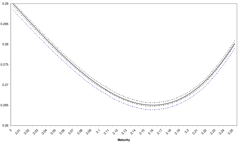
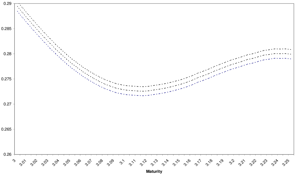
Implied volatilities resulting from
interpolation by daycount fractions vs. interpolation with short bond volatility
6. Broken Date Caplets: A Comparison
Another point of interest is how the choice of interpolation method affects the pricing of derivatives. In this context, the volatility of interpolated rates is of key importance. When extending the discrete tenor model to continuous tenor, one is faced with a tradeoff of completing the model via volatilities or interest rate interpolation. By fixing the volatilities of rates for all maturities, say all –compounded forward LIBORs , as in MSS and BGM, the model is completely specified and there is no need to interpolate interest rates. On the other hand, when the interpolated rates are given as functions of the discrete tenor forward LIBORs, their volatilities can be calculated by an application of Ito’s Lemma. The former approach has the disadvantage of rather intractable dynamics for rates other the –compounded forward LIBORs, while latter implies that the “broken date” forward LIBORs , are not lognormal. Applying Ito’s Lemma to (13), the relative volatility of is
For method 1 this becomes
Figures 7 and 7 illustrate how the two interpolation methods presented in the previous sections affect the prices for “broken date” caplets. In each plot, we vary the maturity of the forward LIBOR underlying the caplet within one –accrual period of the discrete tenor structure (i.e. the caplets on the two endpoints of each plot are based on non-interpolated rates). The strike is chosen at 1.25 times the at–the–money level and the volatility function is two–dimensional exponentially decaying.151515For details see appendix. This choice should provide a representative example well away from the trivial at–the–money, one–dimensional constant volatility case. The caplet prices were generated by Monte Carlo simulation; the middle line in each plot give the Monte Carlo estimate, while the outside lines are the confidence interval boundaries two standard deviations to either side of the Monte Carlo estimate. One million MC runs make these confidence bounds reasonably tight. We represent the caplet prices in terms of their Black/Scholes implied volatility, i.e. in terms of the one–dimensional constant relative volatility of the underlying rate which would result in the same caplet price. The dip in the implied volatilities is due to the fact that the interpolation of at maturity of the caplet is in part based on , i.e. a rate which evolves stochastically only until . This effect is less pronounced under interpolation with short bond volatility, as in this case plays a lesser role.
The disadvantage that the “broken date” forward LIBORs are not lognormal is greatly alleviated by the fact that their distribution is actually very close to lognormal. One can apply the argument which was first used to derive an approximate swaption formula in a lognormal forward LIBOR model.161616This argument first appears in ? (?). It was developed further in ? (?) and formalized by ? (?). This approximation works well not only for pricing, but also for hedging, as demonstrated in ? (?). Noting that the level dependence of the volatility of the interpolated forward LIBORs varies slowly compared to the rates themselves, one can derive an approximate closed–form solution for the “broken date” caplet by calculating the level dependence with respect to the initial rates, e.g. for method 1 by setting
The Black/Scholes implied volatility is then given by
with
As illustrated by Figure 7, the resulting approximation of Black/Scholes implied volatilities is very accurate.
7. Conclusion
Extending the models of market observable interest rates from discrete to continuous tenor by interpolation is particularly useful in implementations where there are some financial products which must be priced numerically, as the Markovian structure of the discrete tenor model is preserved. It is important to note that the interpolation method cannot be chosen arbitrarily for all maturities. Rather, it must take into account the relevant no–arbitrage conditions.
Shifting the focus from instantaneous forward rates to market observables such as forward LIBOR, the rate dynamics implied by the proposed interpolation methods are reasonable. These methods supply alternatives to the continuous tenor versions of the lognormal forward rate Market Models proposed in the literature and in those cases where moving to continuous tenor by interpolation entails a loss of tractability, for example for “broken date” caplets, very accurate approximations exist.
Appendix: Model Parameters
To generate the plots, two volatility specifications and were used:
The length of the discrete tenor accrual period is in all cases 0.25.
Initial Fixed Figure Term Volatility Fixed Time to Structure Maturity Maturity 2 1 10 NA NA 2 1 10 NA NA 3 2 10 NA NA 4 3 2.25 1.8125 0.3125 5 3 2.25 1.8125 0.3125 7 3 4.25 NA NA 7 3 4.25 NA NA
Three initial term structures of discrete tenor forward LIBORs are considered:
-
(1)
Linearly increasing from 4% at 0 years up to 6% at 5 years and then linearly decreasing down to 4% at 10 years.
-
(2)
Linearly increasing from 5% at 0 years up to 6.7% at 4.25 years, then linearly decreasing to 6.5% at 4.75 years, then linearly increasing to 6.8% at 5.5 years, and then linearly decreasing down to 5% at 10 years.
-
(3)
Linearly increasing from 5% at 0 years up to 10% at .
References
- [1]
- [2] [] Andersen, L. and Andreasen, J. (1998), Volatility Skews and Extensions of the LIBOR Market Model, General Re Financial Products, working paper .
- [3]
- [4] [] Black, F. (1976), The Pricing of Commodity Contracts, Journal of Financial Economics 3, 167–79.
- [5]
- [6] [] Black, F. and Scholes, M. (1973), The Pricing of Options and Corporate Liabilities, Journal of Political Economy pp. 637–654.
- [7]
- [8] [] Brace, A. and Womersley, R. S. (2000), Exact Fit to the Swaption Volatility Matrix Using Semidefinite Programming, ICBI Global Derivatives Conference, working paper .
- [9]
- [10] [] Brace, A., Dun, T. and Barton, G. (1998a), Towards a Central Interest Rate Model, Conference Global Derivatives ’98, working paper .
- [11]
- [12] [] Brace, A., Gatarek, D. and Musiela, M. (1997), The Market Model of Interest Rate Dynamics, Mathematical Finance 7(2), 127–155.
- [13]
- [14] [] Brace, A., Musiela, M. and Schlögl, E. (1998b), A Simulation Algorithm for Lognormal Market Models, FMMA, working paper .
- [15]
- [16] [] Corr, A. (2000), Finite Dimensional Representability of Forward Rate and LIBOR Models, PhD thesis, School of Mathematics, University of New South Wales.
- [17]
- [18] [] Dun, T., Barton, G. and Schlögl, E. (2001), Simulated Swaption Delta–Hedging in the Lognormal Forward LIBOR Model, International Journal of Theoretical and Applied Finance 4(4), 677–709.
- [19]
- [20] [] El Karoui, N., Lepage, C., Myneni, R., Roseau, N. and Viswanathan, R. (1991), The Valuation and Hedging of Contingent Claims with Markovian Interest Rates, Université de Paris 6, working paper .
- [21]
- [22] [] Heath, D., Jarrow, R. and Morton, A. (1992), Bond Pricing and the Term Structure of Interest Rates: A New Methodology for Contingent Claims Valuation, Econometrica 60(1), 77–105.
- [23]
- [24] [] Ho, T. S. and Lee, S.-B. (1986), Term Structure Movements and Pricing Interest Rate Contingent Claims, Journal of Finance XLI(5), 1011–1029.
- [25]
- [26] [] Jamshidian, F. (1997), LIBOR and Swap Market Models and Measures, Finance and Stochastics 1(4), 293–330.
- [27]
- [28] [] Miltersen, K. R., Nielsen, J. A. and Sandmann, K. (2001), The Market Model of Future Rates, University of Mainz, working paper .
- [29]
- [30] [] Miltersen, K. R., Sandmann, K. and Sondermann, D. (1997), Closed Form Solutions for Term Structure Derivatives with Log-Normal Interest Rates, The Journal of Finance 52(1), 409–430.
- [31]
- [32] [] Musiela, M. and Rutkowski, M. (1997), Continuous–Time Term Structure Models: A Forward Measure Approach, Finance and Stochastics.
- [33]
- [34] [] Rady, S. (1997), Option Pricing in the Presence of Natural Boundaries and a Quadratic Diffusion Term, Finance and Stochastics 1(4), 331–344.
- [35]
- [36] [] Rutkowski, M. (1997), Spot, Forward, and Futures LIBOR Rates, Institute of Mathematics, Politechnika Warszawska, working paper .
- [37]
- [38] [] Sandmann, K. and Sondermann, D. (1989), A Term Structure Model and the Pricing of Interest Rate Options, SFB 303, Universität Bonn, working paper B–129.
- [39]
- [40] [] Sandmann, K. and Sondermann, D. (1994), A Term Structure Model and the Pricing of Interest Rate Options, The Review of Futures Markets 12(2), 391–423.
- [41]
- [42] [] Sandmann, K., Sondermann, D. and Miltersen, K. (1995), Closed Form Term Structure Derivatives in a Heath–Jarrow–Morton Model with Log–normal Annually Compounded Interest Rates, Research Symposium Proceedings CBOT pp. 145–164.
- [43]
- [44] [] Schlögl, E. (2002a), Arbitrage–Free Interpolation in Models of Market Observable Interest Rates, in K. Sandmann and P. Schönbucher (eds), Advances in Finance and Stochastics, Springer-Verlag.
- [45]
- [46] [] Schlögl, E. (2002b), A Multicurrency Extension of the Lognormal Interest Rate Market Models, Finance and Stochastics 6(2), 173–196.
- [47]