Gaia-ESO Survey: INTRIGOSS - A new library of High Resolution Synthetic Spectra

Abstract

We present a high resolution synthetic spectral library, INTRIGOSS, designed for studying FGK stars. The library is based on atmosphere models computed with specified individual element abundances via ATLAS12 code. Normalized SPectra (NSP) and surface Flux SPectra (FSP), in the 4830-5400 Å  wavelength range, were computed with the SPECTRUM code. INTRIGOSS uses the solar composition by Grevesse et al. (2007) and four [$\alpha$/Fe] abundance ratios and consists of 15,232 spectra. The synthetic spectra are computed with astrophysical gf-values derived by comparing synthetic predictions with a very high SNR solar spectrum and the UVES-U580 spectra of five cool giants. The validity of the NSPs is assessed by using the UVES-U580 spectra of 2212 stars observed in the framework of the Gaia-ESO Survey and characterized by homogeneous and accurate atmospheric parameter values and by detailed chemical compositions. The greater accuracy of NSPs with respect to spectra from the AMBRE, GES_Grid, PHOENIX, C14, and B17 synthetic spectral libraries is demonstrated by evaluating the consistency of the predictions of the different libraries for the UVES-U580 sample stars. The validity of the FSPs is checked by comparing their prediction with both observed spectral energy distribution and spectral indices. The comparison of FSPs with SEDs derived from ELODIE, INDO–U.S., and MILES libraries indicates that the former reproduce the observed flux distributions within a few percent and without any systematic trend. The good agreement between observational and synthetic Lick/SDSS indices shows that the predicted blanketing of FSPs well reproduces the observed one, thus confirming the reliability of INTRIGOSS FSPs.

1 Introduction

The use of stellar spectral libraries dates back to several decades with some of the most prominent examples being the data set constructed by Jacoby, Hunter, & Christian (1984) and that of Kurucz (1979) which provide examples, respectively, of empirical and theoretical approaches to understand the stellar atmospheres, in particular the photospheres. Over the nearly 40 years since those papers a wealth of works have furnished with very extensive spectral libraries that have (partially) coped with the drawbacks found in the different approaches. On the empirical side, newer databases contain higher resolution spectra (e.g. ELODIE (Moultaka et al., 2004); Sloan Digital Sky Survey (SDSS) as, for example, SEGUE (Yanny et al., 2009) and APOGEE (Majewski et al., 2017); Galactic Archaeology with HERMES (GALAH) survey (De Silva et al., 2015); Gaia-ESO Survey (GES, Gilmore et al., 2012; Randich & Gilmore, 2013); etc.) with a much comprehensive coverage of the parameter space (i.e. in effective temperature, $T_{\rm eff}$, surface gravity, log $g$, and chemical composition, [Fe/H] and [$\alpha$/Fe]), and wavelength. On the theoretical side, current available libraries of theoretical spectra have incorporated more extended line lists and updated atomic and molecular parameters in addition to a more detailed calculation of the radiative transfer equation allowing for departures of the local thermodynamic equilibrium and, in general, including more realistic treatment of the physical processes, e.g. motions, from microturbulence to 3D dynamics of convection, than those that characterize a classical model atmosphere (Hubeny, 1988; Husser et al., 2013, etc).

Stellar libraries have been extensively applied in a number of astrophysical topics as:

• automatic analysis of data in stellar surveys to derive atmospheric parameters, radial and rotational velocities;

• detection of exoplanets via cross-correlation with spectra templates;

• study of star formation history of galaxies by using synthetic and observed photometric indices and/or Spectral Energy Distributions (SEDs).

It is practically impossible to review here the full set of applications, however, the compilation of Leitherer et al. (1996) gives evidence of the use of spectroscopic stellar data sets in the particular case of, perhaps, the most widely spread implementation: studies of galaxy structure and evolution.

It is worthwhile noticing that most of the empirical libraries carry on the imprints of the local properties of the solar neighbourhood hampering the study of stellar populations characterized by star formation history different from that one in our vicinity. Therefore, several theoretical libraries were computed to complement the empirical ones and are available in the literature (e.g. Coelho et al. 2005, C05; de Laverny et al. 2012, AMBRE; Husser et al. 2013, PHOENIX; Coelho 2014, C14; Brahm et al. 2017, B17). As mentioned before, these theoretical libraries can be used to derive stellar atmospheric parameters by comparing observed spectra with their predictions even if some limitations arise from the approximation and inaccuracies in the models and input data used to compute them.

The computation of a theoretical library consists in the calculation of a set of model atmospheres giving the temperature, gas, electron and radiation pressure distributions as a function of column mass or optical depth and the computation of the emerging spectra via a spectral synthesis code. As far as the set of atmosphere models the most commonly used for the analysis of Sun-like stars are those computed with ATLAS9 (Castelli & Kurucz, 2003), ATLAS12 (Kurucz, 2005a), MARCS (Gustafsson et al., 2008), or PHOENIX (Hauschildt & Baron, 1999) codes, while synthetic spectra may be computed with several spectral synthesis codes like DFSYNTHE (Castelli, 2005; Kurucz, 2005a, b), SPECTRUM (Gray & Corbally, 1994), PHOENIX, MOOG, etc.

The available libraries in the literature differ not only because of the different model and synthesis codes used but also because of different adopted chemical mixture and different atomic and molecular line lists. Moreover, not all the libraries provide both normalized High Resolution (HR) spectra and SEDs since they require different approaches (see, for example, the discussion in C14).

A comparison among the performance of existing libraries is given in B17 where the authors presented their synthetic spectra library devoted to the determination of atmospheric stellar parameters via the Zonal Atmospheric Stellar Parameters Estimator (ZASPE). Even if the B17 spectral library is able to obtain results more consistent with the SWEET-Cat catalogue used to validate ZASPE code than C05 and PHOENIX, such a library, adopting solar scale abundances, may introduce systematic biases in the determination of log g values for stars having non solar [Mg/Fe] (see B17). Furthermore, B17 library consists only of normalized HR spectra and therefore is not fully suited for stellar population studies requiring SEDs.

In this paper we present a new library of HR synthetic spectra, INaf-TRIeste Grid Of Synthetic Spectra (INTRIGOSS), for F,G,K stars covering the wavelength range from 4830 to 5400 Å which, even if rather narrow, is very useful to derive stellar atmosphere parameter values for these stellar types. INTRIGOSS spectral library, which is available on the web, aims to furnish a tool for stellar atmosphere parameter determination and it consists of Normalized SPectra (NSP) and surface Flux SPectra (FSP). Model atmospheres and theoretical spectra were obtained assuming as solar composition the one derived by Grevesse et al. (2007) and the full consistency of the library was guaranteed by using ATLAS12 and SPECTRUM v2.76f codes which allowed us to specify the same individual element abundances both in deriving the atmosphere structures and the emerging spectra. The NSPs and FSPs were computed with an atomic and molecular line list built by tuning oscillator strengths in order to reproduce a set of HR reference spectra, namely the Solar spectrum and the GES spectra of five cool giants with high Signal-to-Noise Ratios (SNR $>$ 100). The final line list includes also a sub-set of bona fide predicted lines. The predicted lines (PLs) are calculated absorption lines corresponding to transitions between levels predicted by atomic structure codes but not measured in laboratory and are affected by large uncertainties in their computed intensity and wavelength. We call bona fide PLs those with wavelength positions and oscillator strengths consistent with the features in the HR reference spectra and which can be safely used to compute reliable SEDs. The NSP and FSP spectra are computed with a wavelength sampling of 0.01 Å thus allowing their degradation at any resolving power $R\lesssim$ 240,000.

INTRIGOSS covers in the parameter space the following ranges: $T_{\rm eff}$ 3750$\div$7000 K, log $g$ 0.5$\div$5.0 dex, and [Fe/H] -1.0$\div$+0.5 dex. Furthermore, to also account for stars with non-solar scaled abundances of $\alpha$ elements, four different chemical compositions with [$\alpha$/Fe]=-0.25, 0.00, +0.25, and +0.50 were adopted.

The validity of the line list used in computing INTRIGOSS NSPs and FSPs and the improvement of INTRIGOSS NSP spectra with respect to those of the already available libraries is attested by comparing them with a set of 2212 GES UVES spectra (hereafter UVES-U580 sample) obtained in a setup centered at 580nm (UVES-580) in the framework of the iDR4 release of Gaia-ESO Survey. GES was designed to target all major Galactic components (i.e. bulge, thin and thick discs, halo and clusters), with the goal of constraining the chemical and dynamical evolution of the Milky Way (Gilmore et al., 2012; Randich & Gilmore, 2013). When completed, the survey will have observed with Fibre Large Array Multi Element Spectrograph/UV-Visual Echelle Spectrograph (FLAMES/UVES) a sample of several thousand FGK-type stars within 2 kpc of the Sun in order to derive the detailed kinematic and elemental abundance distribution functions of the solar neighbourhood. The sample includes mainly thin and thick disc stars, of all ages and metallicities, but also a small fraction of local halo stars. Data reduction of the FLAMES/UVES spectra has been performed using a workflow specifically developed for this project (Sacco et al., 2014). The iDR4 release contains radial and rotational velocities, recommended stellar atmosphere parameters, and individual element abundances. It also contains the stacked spectra derived from observations made for the Gaia-ESO Survey during iDR4 and tables of metadata summarizing these spectra. The UVES-580 spectra were analyzed with the Gaia-ESO multiple pipelines strategy, as described in Smiljanic et al. (2014). The results of each pipeline are combined with an updated methodology (Casey et al., in prep.) to define the final set of recommended values of the atmospheric parameters and chemical abundances that are part of iDR4 (see also Magrini et al., 2017).

The validity of the INTRIGOSS FSP spectra is checked by comparing observed and synthetic SEDs for a sub-sample of stars and through the analysis of synthetic photometric indices computed for all the UVES-U580 stars from the corresponding derived FSPs. In particular, in this paper, we show the very good agreement between observational and INTRIGOSS synthetic Mg₁, Mg₂, and Mgb Lick/SDSS indices (Franchini et al., 2010).

In Section 2 we describe how the models and the synthetic spectra were computed, the atomic and molecular line lists we used, and the sample of UVES-U580 spectra adopted as reference to check the reliability of our library. Section 3 compares the predictions of INTRIGOSS with those of publicly available spectral libraries and discusses the achieved improvements. In Section 4 we describe the INTRIGOSS data products and auxiliary files available on the web. Finally, in Section 5 we summarize and conclude.

2 The theoretical library of synthetic spectra: INTRIGOSS

The construction of a theoretical stellar library requires several fundamental ingredients that are applied along different steps. The two main ingredients are: (a) a set of model atmospheres that are needed as input in the calculation of synthetic spectra and (b) a fiducial line list to take into account the relevant individual atomic as well as molecular transitions expected to be important for the parameter space under consideration. Additionally, one requires the appropriate codes for the computations and the choice of the spectrum/spectra to which the theoretical data set will be compared to check the capability of the library in representing real stars.

The construction of INTRIGOSS consists of several steps. The first is the calculation of a grid of model atmospheres that provide the variation of physical quantities throughout the atmosphere. This task has been carried out by using the ATLAS12 code developed by Kurucz (2005a). Once a set of theoretical models has been constructed, the next step is to calculate, under the same considerations (i.e. Local Thermodynamic Equilibrium, LTE), the corresponding synthetic spectra at high resolution. If the input fiducial atomic and molecular line list is adequate to predict line profiles of observed spectra, this would be the second and last step in the process, nevertheless, any working line list actually needs fine tuning of the main agent that affect line intensities, i.e. the oscillator strengths or the log(gf) values, for the (at least) more prominent transitions. This last task is usually conducted by comparing synthetic spectra with observed data of the highest quality. Below we provide details of these processes that end-up with the theoretical library INTRIGOSS.

2.1 The atmosphere models

As discussed in Kurucz (2005a) and Castelli (2005), ATLAS12 can generate an atmospheric model for any desired individual element chemical composition and microturbulent velocity ($\xi$), since the treatment of opacity is based on the Opacity Sampling technique, instead of the Opacity Distribution Functions method used, for example, by ATLAS9. We adopted for the reference solar abundances those obtained from Grevesse et al. (2007) which have a wide consensus in the literature and whose validity is also confirmed, within the quoted uncertainties, by the abundance determinations derived by the Working Group 11 (WG11) of the Gaia-ESO consortium (Magrini et al., 2017) from the analysis of solar and M67 giant UVES spectra obtained with the U580 and U520 setups (Dekker et al., 2000).

We computed sets of atmosphere models in the following ranges of atmospheric parameters:

1. $T_{\rm eff}$ from 3750 to 7000 K at a step of 250 K;

2. log $g$ from 0.5 to 5.0 dex at a step of 0.5 dex;

3. $[$Fe/H$]$ from -1.0 to +0.5 dex at a step of 0.25 dex;

4. $[\alpha$/Fe$]$ from -0.25 to +0.5 dex at a step of 0.25 dex where the $\alpha$ elements considered are O, Ne, Mg, Si, S, Ar, Ca, and Ti;

5. $\xi$ equal to 1 and 2 km s^-1.

Our atmosphere models were calculated by using ATLAS12 and, as initial starting models, the ATLAS9 Model Atmospheres calculated for the APOGEE survey available online. The resulting models computed with the two $\xi$ values, were checked by looking at the behaviors of temperature, gas pressure, electron density, Rosseland absorption coefficient, and radiation pressure at all Rosseland optical depths. The few gaps in the coverage of the resulting atmosphere models in the $T_{\rm eff}$-log $g$ plane correspond to the absence of initial models in the APOGEE set. In running ATLAS12 we used in input atomic and molecular species (file molecules.dat), the lines of all the elements in the first 5 stages of ionization (fclowlines.bin), the lines of diatomic molecules (diatomicsiwl.bin⁵ and tioschwenke.bin by Schwenke 1998), and the lines of H₂O (h2ofastfix.bin) by Partridge & Schwenke (1997). The adopted steps along $T_{\rm eff}$, log $g$, $[$Fe/H$]$, and $[\alpha$/Fe$]$ correspond, roughly, to twice the standard uncertainties in the atmosphere parameter determinations quoted in the literature (see for example Magrini et al. 2017). It is worth noting, that on the basis of the considerations presented in Sections 3.1 and 3.2, a smaller step in temperature would make safer any interpolation required for deriving stellar atmospheric parameters. Therefore, in a future extended version of INTRIGOSS aimed to increase, in particular, its wavelength coverage, we plan to adopt a finer temperature grid.

2.2 The synthetic spectra

To obtain from each atmosphere model the corresponding emergent flux and normalized spectrum we used SPECTRUM v2.76f. SPECTRUM is a stellar spectral synthesis program that calculates, under the LTE approximation, the synthetic spectrum for a given model atmosphere. The code additionally requires line lists of atomic and molecular transitions, that should be as accurate and complete as possible, and supports all expected atomic elements and the following diatomic molecules: H2, CH, NH, OH, MgH, SiH, CaH, SiO, C2, CN, CO and TiO. The code can deliver both the stellar-disk-integrated normalized spectrum and the absolute monochromatic flux at the stellar surface. The user should specify the wavelength range and sampling, the value of microturbulence velocity ($\xi$), and the individual element abundances to be used. For this work we have built a line list by merging the line data used by Lobel (2011, hereafter LO11) and the cool5.iso.lst line list kindly provided to us by R. O. Gray (2011, private communication), complemented with molecular lines of CH, NH, MgH, SiH, C₂, CN, and TiO and with both atomic (in the three main expected stages of ionization) and molecular predicted lines from Kurucz’s site. The lines included in our calculations for the wavelength interval 4830 to 5400 Å are 1427628 including 16531, 339652, and 1071445 transitions for atomic, molecular, and PL entries, respectively.

As indicated previously, accurate astrophysical synthetic spectra computation requires reliable atomic and molecular data, in particular accurate oscillator strength, gf-values, for the transitions expected in the wavelength interval of interest. In recent years a number of online databases (i.e. NIST, VALD, NORAD, the Kurucz website, etc) provide line data from a large variety of sources in the scientific literature. The gf-values given in the databases may either have been determined in the laboratory or derived from theoretical calculations. Thus the accuracy of these gf-values may vary widely from line to line; some are known with accuracies of 1% or better, while others may be off by orders of magnitude. A possible way to reduce these uncertainties is to compare high SNR spectra of stars, with well known atmospheric parameters and abundances, with their corresponding computed synthetic spectra. In this way the gf-values may be checked (and if needed, adapted with a trial-and-error strategy) by looking for a best agreement between the synthetic and observed line profiles thus deriving astrophysical gf-values. Since the line profiles depend both on stellar characteristics, namely $T_{\rm eff}$, log $g$, element abundance, and $\xi$, and on the gf-value, the risk in such an approach is to wrongly adapt the gf-values to compensate for potential inaccuracies in the assumed values of atmospheric parameters and in the modeling assumptions. It is, therefore, important to perform the comparison of the synthetic and observed profile of the same line in spectra of as many (and as different) as possible stars in order to disentangle the effect of incorrect gf-values from those due to uncertainties in the other parameters.

In this context, Lobel (2011, hereafter LO11) used the high-resolution spectrum of three main sequence stars, the Sun, Procyon, and $\epsilon$ Eri, characterized by the following $T_{\rm eff}$, log $g$, and $\xi$ values: SUN (5777,4.438,1.1), Procyon (6550,4.0,1.2), and $\epsilon$ Eri (5050,4.5,0.55) and assuming solar composition from Anders & Grevesse (1989) also for the last two stars. He used the solar spectrum observed in 1981 with the NSO/KPNO Fourier Transform Spectrograph (FTS), degraded at R$\sim$80,000, and, for Procyon and $\epsilon$ Eri, several optical spectra taken with the Hermes spectrometer on the 1.2 m Mercator telescope at La Palma Observatory, Canary Islands. The comparison synthetic spectra were calculated with the LTE radiative transfer SCANSPEC code and, in such a way, LO11 updated the log(gf) values of 911 neutral lines in the wavelength range 4000$\div$6800 Å. The main causes of uncertainties in the LO11 results arise from: i) the problems of deriving the solar intensity (averaged over the solar disk) from the NSO/KPNO Fourier Transform observations; ii) the assumption of solar composition for Procyon, and $\epsilon$ Eri even if some differences in individual element abundances are reported in the literature (see for example Jofré et al., 2015); iii) the use of only relatively high temperature ($T_{\rm eff}>$ 5000 K) main sequence stars which does not allow to check the log(gf) values of those atomic and molecular lines that are mainly prominent in giants and/or cooler stars.

We decided to complement the LO11 work by performing the same kind of analysis but by using an ad hoc derived high SNR solar spectrum and the UVES-U580 spectra with SNR above 100 of five giant stars (see Table 1) with atmospheric parameters in the following ranges: $T_{\rm eff}$ between 4500 and 5000 K, log $g$ from 2.0 to 3.2 dex, and $\xi$ from 1.0 to 1.5 km s^-1, and, for each star, the individual element abundances derived by GES Consortium and reported in the GESiDR4Final catalogue (Magrini et al., 2017).

The outline of our method is the following:

• use of the solar spectrum as the main reference to derive the astrophysical log(gf) values for atomic and molecular lines that are important at solar effective temperature and gravity by assuming no uncertainties in the solar parameters and in the adopted atmosphere model;

• use of the five giant spectra to derive the astrophysical log(gf) values of those lines that are more prominent at temperatures and gravities lower than the solar ones and to fix globally the MgH opacity by using the scaling factor f_MgH (see Section 2.2.2);

• use of a large sample of stars (more than 2200) covering a wider range of atmospheric parameter values to validate the final list of astrophysical log(gf) values.

2.2.1 Refinement of oscillator strengths and tuning of the central wavelengths: The solar case

We used an observed solar spectrum which is the average of 59 integrated sunlight spectra, as reflected by the Moon, taken with HARPS spectrograph at the 3.6-m La Silla European Southern Observatory (ESO) telescope. These spectra are the out-of-transit sub-sample of those taken to detect the Rossiter-McLaughlin effect in the Sun due to the Venus transit of 2012 June 6 (Molaro et al., 2013). The SNR of the average spectrum, as evaluated by looking at the ratio between the mean flux and the standard deviation of the mean at each wavelength, is about 4000. Then the spectrum was degraded at the resolution of the Hermes spectra (R=80,000).

The normalized synthetic solar spectrum to be used in the comparison was computed with SPECTRUM starting from the ATLAS12 model obtained with $T_{\rm eff}$=5777 K, log $g$=4.4377 dex, $\xi$=1.0 km s^-1, and with the solar abundances by Grevesse et al. (2007). This spectrum was then degraded at R=80,000 and convolved with the geometric mean of the solar $v\sin i$ and macroturbulence velocity values (2.5 km s^-1).

Prior to conducting modifications on the line data we first need to normalize the observed spectra, a crucial process to derive reliable log(gf)s. With the goal of matching the continuum levels of observed and synthetic spectra, we searched for continuum flux reference points in the normalized synthetic spectrum and identified the wavelength intervals with flux levels in excess of 0.99, avoiding, in this way, regions with absorption lines where the uncertainties in the log(gf) values may play a role. Then, the observed spectrum in each of the corresponding wavelength regions is divided by the synthetic one and these ratios are fitted with a polynomial. Eventually, the observed spectrum is divided by the so computed polynomial to obtain the normalized spectrum.

A trial-and-error procedure based on the comparison between the normalized and the synthetic solar spectrum is now applied to modify (when needed) the input log(gf) values and/or the central wavelengths in order to match the profile of the observed lines or blends. We compared our observed and synthetic solar spectra to adapt the log(gf)s of those lines which are responsible of clearly detectable flux minima in the observed and/or synthetic spectra to obtain their astrophysical values. We followed a three steps approach:

1. we looked in our input line list to identify the transitions responsible for those minima present in both the observed and synthetic spectra and we iteratively modified their log(gf) values until we found a satisfactory agreement. In general we stopped the iteration when the difference between synthetic and observed spectra were below $\pm$ 0.003;

2. we selected the minima present only in the synthetic spectra and reduced the log(gf) values of the corresponding theoretical lines to match the observed spectrum;

3. we searched in our input line list and in the online databases listed in Section 2.2 for theoretical lines which may correspond to minima present only in the observed spectrum and, for those lines found, we fine tuned their log(gf) values and added them to our input list if needed.

In all the above listed steps we also checked the central wavelength of each identified features and, in a few cases, we slightly modified it to better match the observed spectrum. Eventually, the identification of the lines corresponding to the minima was double-checked by looking at the same wavelength regions in the synthetic and observed spectra of five giants (see Section 2.2.2).

In conclusion we derived astrophysical log(gf) values for 2229 lines, that include 850, 35, and 1344 atomic, molecular, and predicted transitions, respectively. The 850 atomic lines include 100 lines from LO11 that required slight modification of their log(gf)s or of their central wavelength to get a better match of the spectra. These corrections are mainly due to the slightly different solar abundances adopted, by the higher SNR of our solar spectrum and by the inclusion in our synthetic spectrum of molecular and predicted lines non present in the SCANSPEC spectra of LO11.

2.2.2 Refinement of oscillator strengths: five giant stars

The above procedure should, in principle, be sufficient to calculate fiducial theoretical spectra that represent stars with atmospheric parameters close to solar. However, to account for potential targets of lower temperature and surface gravity one needs to extend the log(gf) tuning analysis to giant stars. For this extension we considered the five giants in Table 1.

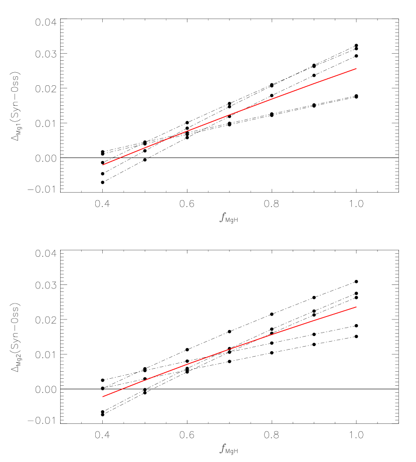
Figure 1: Differences between synthetic and observed Mg₁ and Mg₂ Lick/SDSS indices for the five giant stars in Table 1 (black dot-dashed thin lines) and their average values (red thick line) as a function of the $f_{\rm MgH}$ value used in computing the synthetic spectra (see text).

We computed for each i-th star its synthetic spectrum (S_i) by using the GES atmospheric parameter values, the individual element abundances and the line list which includes the astrophysical log(gf)s derived from the solar spectrum analysis. Then, we adopted the same procedures used for normalizing the observed solar spectrum for each i-th giant to derive from its UVES-580 spectrum the normalized one (O_i). First of all we checked that the modified log(gf) values obtained in Section 2.2.1 provide a good agreement of synthetic and observed spectra also for these five stars. We adopted as acceptance threshold a value of $\pm 0.01$ which is larger than that one used for the Sun due to the lower resolution (R=47,700) and SNR ($\sim 100$). Actually, in all but a very few cases, we did not need to go back to the analysis of the solar spectra to re-tune the log(gf)s. Then, we looked for features which were present only in the spectra of the giants. By adopting the same trial-and-error strategy used for the solar case but the new acceptance threshold we were able to derive astrophysical log(gf) values for an additional number of 175 lines, namely 49, 42, and 84 atomic, molecular, and predicted transitions, respectively. As far as the large number of weak lines of MgH, which is the dominant molecular opacity contributor in our wavelength range, are concerned we decided to check individually, for this molecule, only the log(gf)s of the strongest features. The contribution of the other MgH lines was then fine-tuned by means of a scaling factor, f_MgH, by which their gfs are multiplied (see SPECTRUM documentation). To evaluate the most appropriate value of f_MgH we computed the Lick/SDSS Mg₁ and Mg₂ indices (Franchini et al., 2010), which are strongly affected by the MgH lines, from the UVES-U580 spectra and compare them with those from synthetic spectra calculated with f_MgH in the range 1.0$\div$0.4. Figure 1 shows that, on the average, the best agreement is obtained with f_MgH=0.45.

It is important to remark that, should we consider that the need of such a low f_MgH is ascribed to uncertainties in the Mg abundances, one would require to decrease the Mg abundances, log(Mg/H), of all the five giants by $\sim$0.35 dex in order to keep the f_MgH value at 1.0. On the other hand, such a low Mg abundances are inconsistent with those derived from the analysis of atomic Mg lines. Therefore, we are confident that the obtained f_MgH=0.45 is not due to a wrong GES Magnesium abundance determination but to an overestimate of the MgH opacities computed by Kurucz (2014) as also found and discussed by Weck et al. (2003). Thus, hereafter we adopted the value f_MgH=0.45 to correct such overestimate and to be consistent with the log(Mg/H) derived from atomic lines.

Table 1: Giant stars used to derive astrophysical log(gf) values

Cname	$T_{\rm eff}$	$\sigma_{T_{\rm eff}}$	log $g$	$\sigma_{{\rm log}\,g}$	[Fe/H]	$\sigma_{\rm[Fe/H]}$	$\xi$	$\sigma_{\xi}$	$V_{\rm rad}$	$\sigma_{V_{\rm rad}}$	$v\sin i$	$\sigma_{v\sin i}$	SNR
	K	K	dex	dex	dex	dex	km s-1	km s-1	km s-1	km s-1	km s-1	km s-1
00241708-7206106	4510	117	2.10	0.23	-0.70	0.10	1.34	0.08	2.91	0.57	2.15	2.82	108
00251219-7208053	4513	114	2.04	0.23	-0.67	0.10	1.45	0.03	-34.30	0.57	2.12	2.61	105
00240054-7208550	4541	121	2.06	0.23	-0.71	0.09	1.40	0.07	-13.13	0.57	2.10	2.56	108
02561410-0029286	4834	117	2.75	0.21	-0.70	0.09	1.05	0.05	-68.65	0.57	2.39	2.85	113
03173493-0022132	4966	121	3.14	0.23	-0.63	0.10	1.03	0.07	-40.28	0.57	2.22	2.51	113

Note. — Atmospheric parameter values from the recommended parameters and abundances table in the GESiDR4Final catalogue

2.3 Assessment of the quality of the modified line list

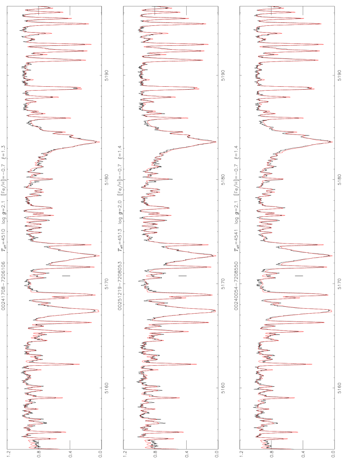
Figure 2: Example of the comparison between the observed spectra (black lines) and the synthetic ones (red lines) computed by using the derived astrophysical log(gf) for the first 3 giant stars in Table 1. As an example of unidentified lines the feature at 5170.77 is indicated (vertical bar).

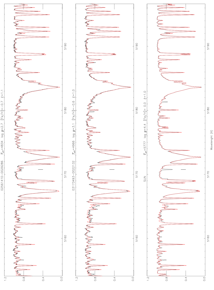
Figure 3: Example of the comparison between the observed spectra (black lines) and the synthetic ones (red lines) computed by using the derived astrophysical log(gf) for the last 2 giant stars in Table 1 and for the Sun. As an example of unidentified lines the feature at 5170.77 is indicated (vertical bar).

Figures 2 and 3 show an example of the agreement between observed and synthetic spectra achieved by using the above-derived astrophysical log(gf)s. For the solar case, in which the uncertainties of the observed spectrum are negligible, a quantitative estimate of the improvement with respect to the use of the initial log(gf) list is given by the decrease of the standard deviation of the residuals from $\sim 0.06$ to $\sim 0.03$. In the case of the five giants, where observational uncertainties must be taken into account, we calculated, as a figure of merit, $r^{\rm i}_{med}=median[(\frac{{\rm O_{i}}(\lambda)-{\rm S_{i}}(\lambda)}{\Delta{\rm O_{i}}(\lambda)})^{2}]$, where $\Delta{\rm O_{i}}(\lambda)$ were obtained from the inverse variance-per-pixel given in the UVES-U580 FITS files. In computing $r^{\rm i}_{med}$ we excluded those wavelength regions which were used to normalize the O_i because they are bound to near-zero residuals and are not sensitive to the quality of the used log(gf)s. We decided to use the median of the normalized residuals instead of the mean because the latter is strongly affected by the residuals in the region of unidentified lines. As can be seen in Table 2 the use of the astrophysical log(gf)s allows us to achieve a 30% decrease of the $r_{med}$ values with respect to the initial ones.

Table 2: Comparison of $r_{med}$ values for the five giants in Table 1 when using initial or astrophysical log(gf)s

Cname	$r_{med}$	$r_{med}$	ratio
	astrophysical	initial	%
00240054-7208550	1.46	2.10	69
00241708-7206106	1.30	1.84	71
02561410-0029286	1.33	1.96	68
00251219-7208053	0.89	1.37	65
03173493-0022132	0.76	1.14	67

We want to point out that some discrepancies still persist, in limited narrow wavelength regions, due to the presence in the observed spectra of lines that we were not able to find in any of the atomic and molecular databases available in literature and, thus, being unidentified cannot be present in the synthetic spectra. A clear example of this situation is the feature at 5170.77 Å  that is present in all observed spectra (see Figures 2, 3 and Table 4), and particularly prominent in the solar one. In Appendix A we list the unidentified observed features.

2.4 Validation of line list improvements on the GES sample

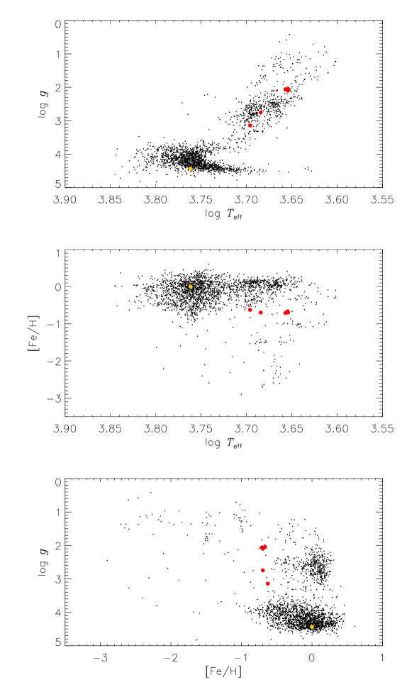
Figure 6: GES atmospheric parameters of the 2212 stars in the UVES-U580 sample (black points) with superimposed those of the Sun (yellow circle) and of the five giants in Table 1 (red circles).

To check the validity of our line list and, as a consequence, of the synthesized spectra over the full atmospheric parameter space covered by F,G, and K stars we decided to use a large sample of stars with well known atmospheric parameter values and individual element abundances. On what follows, we will use the observed spectra of 2212 UVES-U580 stars extracted from the forth Gaia-ESO (iDR4) release, whose atmospheric parameter coverage is shown in Figure 6, in order to compare them with the corresponding individual NSP synthetic spectra. Our check is based on the important remark that, if we had derived wrong gf-values from the spectra of the Sun and of the five stars in Table 1 because of errors in the adopted stellar atmosphere parameters, these gf-values should be very ineffective in reproducing the observed spectra of stars covering a much more extended parameter space. Furthermore, we have to point out that any coupling between our astrophysical gf-values and GES atmospheric parameter determinations is very unlikely since our main reference star in deriving astrophysical gf-values is the Sun (whose adopted atmospheric parameter values were not from GES). Moreover, the GES atmospheric parameter values of the five giants in Table 1 are the homogenized results of several Working Group and Nodes of the Gaia-ESO consortium and are not at all related to the process conducted in this work for calculating theoretical models and spectra.

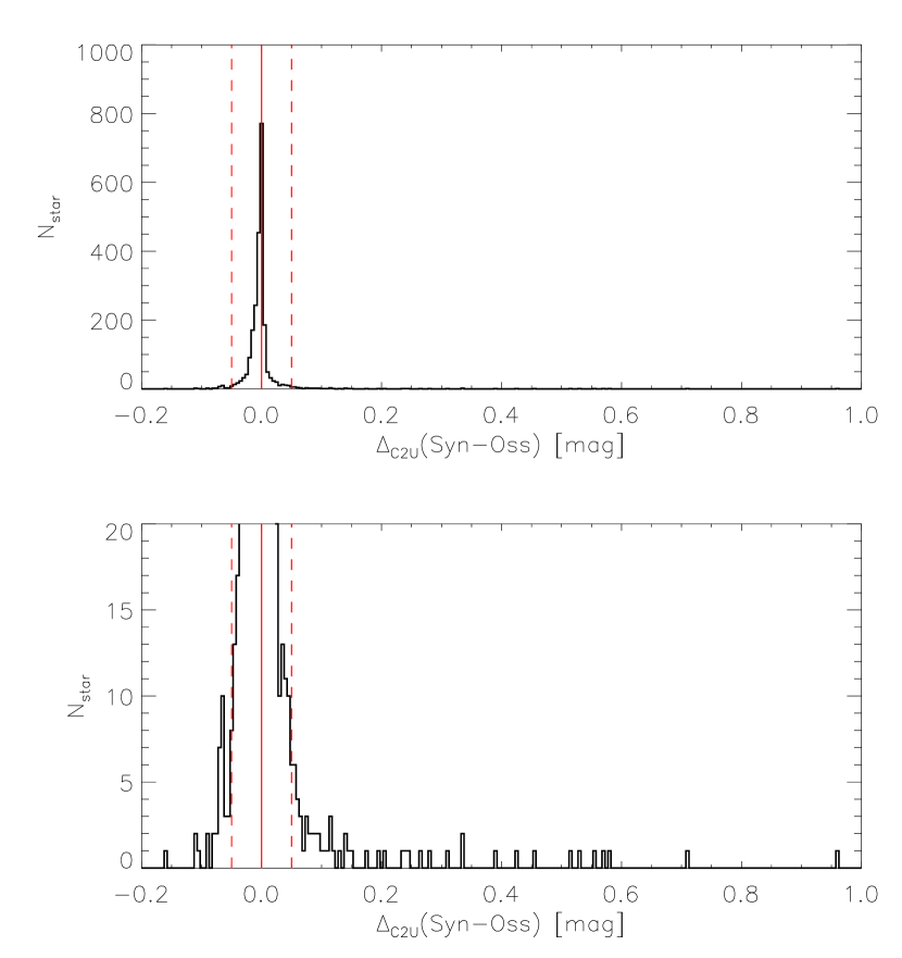
Figure 4: Distribution of the differences between C2U indices derived for each pair of synthetic and UVES-U580 spectra; the lower panel shows, by zooming the y-scale, the presence of several outliers. Stars with $\Delta_{\rm C2U}$ values outside the red dashed lines ($\pm 0.05$ mag) are removed from the UVES-U580 sample (see text).

A first sample of 2616 stars was obtained by performing an SQL search to select all the stars in the 3500-7000 K and 0.25-5.25 dex effective temperature and surface gravity ranges observed with U580 setup and characterized by a Signal to Noise Ratio (SNR) greater than 10. Then, we removed all the stars with some peculiarity flag and/or lack of an error estimate of the stellar atmosphere parameters. In such a way we obtained a sample of 2311 stars well suitable for our analysis since it contains objects with homogeneously determined $T_{\rm eff}$, log $g$, detailed chemical composition, $\xi$, and $v\sin i$ spanning the following ranges: $T_{\rm eff}$ from 3900 to 7000 K; log $g$ from 0.4 to 4.9 dex; $[$Fe/H$]$ from -2.9 to +0.6 dex; $[\alpha$/Fe$]$ from -0.1 to +0.6 dex; and $\xi$=0.1–3.0 km s^-1. For each i-th star we run ATLAS12 and SPECTRUM codes, using its GES atmospheric parameter values, individual element abundances (for those elements with no estimate of [X/Fe] we assumed [X/Fe]=0) and our modified line list, to compute the appropriate normalized synthetic spectrum (S_i) which is then used to obtain from the corresponding observed (stacked) UVES-U580 spectrum a normalized one (O_i). The normalization was performed by applying the same technique as for the solar spectrum. In few cases the S_i resulted to be significantly different from the O_i, in particular below 5167 Å. This region includes the C₂ bands of the Swan system (Swan, 1957) and, in particular the one used by Gonneau et al. (2016, Table 2) to define the C2U index, thus suggesting that the mismatch between S_i and O_i may be related to differences in the estimated and actual stellar Carbon content. The abundance determination of C is quite challenging and the values of [C/Fe] derived by GES are, in general, less accurate than for the other elements. In particular, GES does not include carbon abundances for 254 stars and, in almost all the other 2057 cases, the estimated [C/Fe] is based on the analysis of only 2 (1572 stars) or even 1 (478 stars) spectral lines. To further investigate the role of [C/Fe] in the comparison of our synthetic spectra with the observed ones we computed for the whole sample of UVES-U580 stars the C2U index from both S_i and O_i. Figure 4 shows that, while in most cases the observed and synthetic C2U indices agree between $\pm 0.05$ mag, there are 99 stars which show larger differences suggesting that their estimated (or assumed) [C/Fe] are not correct. As a consequence, these stars are, for precaution, removed from our UVES-U580 sample which, at the end, consists of 2212 stars with normalized observed spectra and NSPs.

In order to quantitatively estimate the agreement between each pair of S_i and O_i within the working GES sample, we calculate the same figure of merit, $r^{\rm i}_{med}$, used to compare the O_i and S_i spectra of the five giants in Table 1. The use of $r^{\rm i}_{med}$ as an estimate of the accuracy of our synthetic spectra requires, however, that we take into account that its value also depends on the uncertainties in the GES atmospheric parameters and in the normalization procedure. In order to investigate these two contributions we computed for each star, in addition to the figure of merit derived from synthetic spectra for the nominal set of GES atmospheric parameters and elemental abundances (that we call n_$r^{\rm i}_{med}$), the synthetic spectra and the figure of merit by adding or subtracting for each atmospheric parameter the given 1-$\sigma$ uncertainty. Note that we have also obtained for each new S_i the corresponding normalized observed spectrum O_i.

The goodness of the GES estimates is confirmed by the general increase of $r^{\rm i}_{med}$ values with respect to the nominal ones when the S_is are computed considering the parameter uncertainties. We found that the main mean increase is caused by the adoption of $T_{\rm eff}-\sigma_{T{\rm eff}}$ and amounts about 10%. The effects of varying the other parameters and of the normalization procedure turned out to be negligible.

The resulting distribution of the n_$r^{\rm i}_{med}$ is presented in the top panel of Figure 5 which shows that the reliability of the astrophysical gf-values in our list and, therefore, of the resulting synthetic spectra, is validated by the small n_$r^{\rm i}_{med}$ values for the bulk of the 2212 stars. In fact, as can be seen, the n_$r_{med}$ distribution is strongly peaked at values below 1, with the maximum of the distribution between 0.6 and 0.7, attesting that, in most cases, the differences between S_i and O_i are on the same order (or even lower) of the estimated observational errors. The presence of a wing in the distribution towards higher n_$r_{med}$ values is mainly due, as expected, to the coolest stars as can be seen in the second panel of Figure 5 where the median values of the n_$r^{\rm i}_{med}$ in partially overlapping bins containing 51 stars each ($\tilde{r}_{med}$) are plotted versus $T_{\rm eff}$. Actually, for these objects, a lower accuracy of our synthetic spectra in reproducing the observed ones is somehow unavoidable due to both the difficulties in computing their atmosphere models and the absence, in our computations, of the tri-atomic molecular lines. In the third and fourth panels we depict the trends of $\tilde{r}_{med}$ vs log $g$ and $[$Fe/H$]$, respectively. The increase of $\tilde{r}_{med}$ for log $g$ between 2.0 and 2.4 dex probably reflects the high number of cool GES stars in this gravity interval. The increase of $\tilde{r}_{med}$ at $[$Fe/H$]\gtrsim 0$ can plausibly be attributed to the insufficient improvement (or lack of it) of the log(gf)s of weak lines in the solar and giant stellar spectra that are more prominent in the super-metal-rich regime.

In conclusion we derived and validated astrophysical gf-values for 899, 77, and 1428 atomic, molecular and predicted lines, respectively. In particular, by adapting also the log(gf) values of PLs, we minimized both the unavoidable underestimation of the blanketing in the synthetic spectra if PLs are ignored (see discussion in C14) and the risk of worsening the match with the observed spectrum if PLs with incorrect intensity are used (see Figure 3 in Munari et al., 2005). Therefore, on the basis of the above discussion, we confidently computed synthetic spectra for each of the ATLAS12 model listed in Section 2.1 and generate the final INTRIGOSS library.

The INTRIGOSS spectral library and the linelist used to compute the synthetic spectra are available online together with auxiliary data as described in Section 4.

3 Comparison with other spectral libraries

One of the main applications of stellar spectral libraries is the automatic analysis of spectra in stellar surveys to derive atmospheric parameters. Several examples can be found in the literature by using different spectral libraries and numerical codes, see for example García Pérez, et al. (2015), Worley et al. (2016), B17, Kos et al. (2017), etc. The accuracy of the obtained atmospheric parameters depends both on the reliability of the input spectral libraries and on the algorithms implemented in the numerical codes used to derive them. It is therefore necessary to remove the effect of the different parameter estimate codes if we want to compare the spectral libraries. Thus we decided to use as reference the UVES-U580 stars together with the homogeneously derived set of GES atmospheric parameter values that we consider as one of the best currently available. Therefore, the comparison of observed stellar spectra with the theoretical predictions of any synthetic stellar libraries can be safely performed by using these GES parameter values as input. In order to perform such a comparison we downloaded the following spectral libraries available on-line: AMBRE, GES_Grid, PHOENIX, C14, and B17. To make a fair comparison, since we could not compute for each UVES-U580 star the corresponding nominal synthetic spectra from the literature libraries, we adopted the following approach: within the six (j) libraries and INTRIGOSS we computed the corresponding synthetic spectrum for each UVES-U580 star by linearly interpolating in $T_{\rm eff}$, log $g$, [Fe/H], $<$[$\alpha$/Fe]$>$ or [Mg/Fe], and $\xi$ at the nominal GES atmospheric parameter values. The interpolation procedure implies the addition of (systematic) errors that will depend on two main factors: the spacing in the grid nodes and the applied interpolation strategy (see for example Mészáros & Allende Prieto, 2013). Whilst a full analysis of the effects of interpolating within INTRIGOSS is beyond the scope of this paper, we hereafter provide some tests to estimate the errors associated with our linear interpolation.

In order to evaluate the errors introduced by our interpolation procedure we computed by using INTRIGOSS prescriptions the intra-mesh atmosphere models and the corresponding synthetic spectra, NSPs and FSPs, of 50 representative UVES-U580 stars, i.e. by using their nominal GES $T_{\rm eff}$, log $g$, [Fe/H], $<$[$\alpha$/Fe]$>$, and $\xi$, but not their individual element abundances. For each star we computed the mean value and the standard deviation ($\sigma_{\rm rd}$) of the relative differences between the interpolated and the intra-mesh spectra. The mean relative differences can be used to evaluate the interpolation error introduced in the overall spectrum levels while the standard deviations can be seen as an estimate of the “noise” introduced point-by-point. In the following Sections 3.1 and 3.2 we will use these values to provide estimates of the interpolation errors introduced by interpolating NSPs and FSPs, respectively.

3.1 The normalized synthetic spectra, NSPs

We used the synthetic spectra obtained by interpolating the different j spectral libraries to normalize the corresponding UVES-U580 spectra and to compute the $r^{j}_{med}$ figure of merit as described in Section 2.2. Due to the different wavelength and parameter space coverage of the six libraries, namely INTRIGOSS, AMBRE, GES_Grid, PHOENIX, C14, and B17, we restricted our analysis to the regions in common, i.e. 4900-5370 Å, and -1.0$\leq$ [Fe/H] $\leq$ 0.5 dex, but for C14 which is limited to [Fe/H] $\leq$ 0.2 dex.

Table 3: Median values of the normalized $r_{med}$s for different spectral libraries

Library	INTRIGOSSMg	INTRIGOSSα	AMBRE	GES_Grid	PHOENIX	C14	B17
$R_{med}$	1.043	1.025	1.313	1.266	2.161	1.700	1.298
$\sigma$	0.003	0.003	0.021	0.011	0.033	0.021	0.014

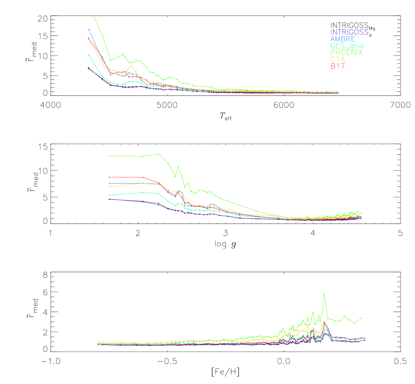
Figure 7: Trends of the median values of the computed $r^{\rm j}_{med}$s for the different spectral libraries (identified by different colours) versus GES $T_{\rm eff}$, log $g$, and [Fe/H] (top to bottom); see text and Figure 5.

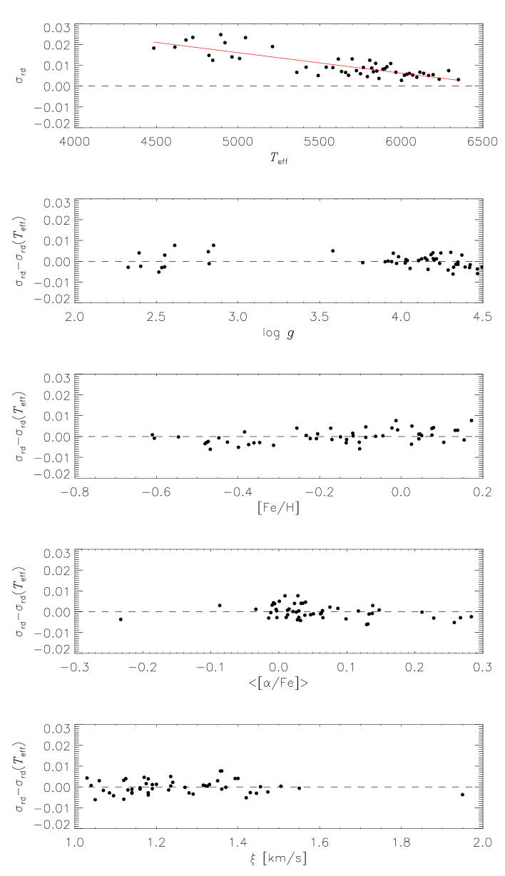
Figure 8: Trends of the standard deviation ($\sigma_{\rm rd}$) of the relative differences between the 50 interpolated and intra-mesh NSPs versus $T_{\rm eff}$, log $g$, [Fe/H], $<$[$\alpha$/Fe]$>$, and $\xi$. The general trend of $\sigma_{\rm rd}$ versus $T_{\rm eff}$, $\sigma_{\rm rd}(T_{\rm eff})$, as derived by a linear regression (red line in the top panel), has been subtracted from $\sigma_{\rm rd}$ in the other panels.

Figure 7 shows the trend of the $\tilde{r}^{j}_{med}$ for the different spectral libraries versus GES $T_{\rm eff}$, log $g$, and [Fe/H]. Table 3 summarizes, for each $j$-spectral library, the variations of $r^{j}_{med}$s with respect to the nominal ones, as evaluated by computing $R^{j}_{med}$=median($\frac{r^{j}_{med}}{n\_r_{med}}$), i.e. the median value of the normalized $r_{med}$s. As can be seen, the use of synthetic spectra computed at the $T_{\rm eff}$, log $g$, [Fe/H], [Mg/Fe] or $<$[$\alpha$/Fe]$>$, and $\xi$ by interpolating the INTRIGOSS library leads to a general increase of a few percents of their $r_{med}$s with respect of the corresponding n_$r_{med}$s thus confirming that the best agreement with the observed spectra can be reached, in general, by using ad-hoc models and the individual element abundances instead of the average metallicity and the average abundance ratio of the $\alpha$-elements. Table 3 shows that slightly better results are obtained by interpolating according to the $<$[$\alpha$/Fe]$>$ stellar value instead of using [Mg/Fe] indicating that, even if one of the major contributors to absorption in this wavelength range is Mg (and MgH), also the behaviour of all the other $\alpha$-elements plays a not negligible role and must be properly taken into consideration. The increase of $r_{med}$s also contains the contribution introduced by the interpolation among the INTRIGOSS grid nodes. By comparing the 50 intra-mesh normalized synthetic spectra (see Section 3) with the corresponding interpolated ones, we found that the mean relative differences are on the order of $\pm 0.1$% showing that the interpolation does not introduce significant inaccuracies in the overall normalized spectrum levels. As far as the relative standard deviations are concerned, top panel of Figure 8 shows that $\sigma_{\rm rd}$ increases with decreasing temperature showing that for $T_{\rm eff}\gtrsim 5500$ interpolation errors become visible when working with spectra at SNR $\gtrsim$ 100 ($\sigma_{\rm rd}\simeq 0.01$) while for lower temperatures interpolation errors become significant also for SNR $\sim$ 50 ($\sigma_{\rm rd}\simeq 0.02$). Furthermore, from Figure 8 we can also see that for the other parameters, once the general trend of the standard deviations with $T_{\rm eff}$ is removed (linear fit shown in the first panel of Figure 8), the expected interpolation errors are less than 1% and do not show any significant trend with regard to the parameter values. On the basis of these results we plan to use a finer step in $T_{\rm eff}$ in the future extended version of INTRIGOSS in order to reduce interpolation errors.

As far as the other spectral library are concerned, we point out that the $\tilde{r}^{j}_{med}$ in Figure 7 and the $R_{med}$s in Table 3 obtained with AMBRE, GES_Grid, PHOENIX, C14, and B17 libraries are much larger than those derived by using INTRIGOSS interpolated spectra (both INTRIGOSS_Mg and INTRIGOSS_α). Their values include both the interpolation errors and the effects of the differences in physical assumptions and atomic and molecular line data in the different libraries. Unfortunately, the quantitative estimates of the uncertainties introduced by the interpolation cannot easily be given because we do not have at our disposal the equivalent intra-mesh synthetic spectra for AMBRE, GES_Grid, PHOENIX, C14, and B17 libraries. Furthermore, different libraries have different nodes, sometimes not equally spaced, and these differences may reflect in different interpolation errors. Nevertheless, it is very unlikely that such large $R_{med}$ values as those reported in Table 3 can be due only to the interpolation errors. Thus, we conclude that the differences in the $R_{med}$ values indicates that INTRIGOSS spectra better reproduce the observed spectra of our UVES-U580 sample than the synthetic spectra from the other libraries.

The better performance of INTRIGOSS synthetic spectra can be inferred not only by the low $R_{med}$ values in Table 3 but also by the much smaller spreads of their normalized $r_{med}$ values which reach a maximum of $\frac{r^{j}_{med}}{n\_r_{med}}$=1.6 with only the 10% of points above 1.2. On the other hand, not only the $R_{med}$ values for the other five libraries are higher but also the spreads of the normalized $r^{j}_{med}$s span interval several units wide with 10% of the $\frac{r^{j}_{med}}{n\_r_{med}}$ values above 2.2, 1.9, 4.3, 2.6, 2.2 for AMBRE, GES_Grid, PHOENIX, C14, and B17, respectively. In particular, inspection of Figure 7 shows that the coolest and/or metal richest stars are those characterized by higher $\tilde{r}^{j}_{med}$ values thus confirming that they are the most critical objects.

3.2 The surface flux spectra, FSPs

3.2.1 Comparison of FSPs versus observed SEDs

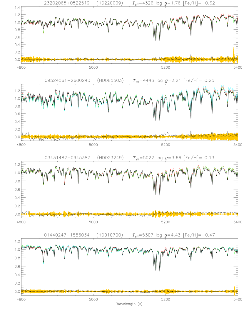
Figure 9: Comparison of flux calibrated spectra (MILES in red, Indo-US in green, and ELODIE in light blue) scaled according to their median values and the corresponding n_FSPs (black). Black curve at the bottom of each panel shows the flux difference, i.e. the average of the observations minus the correspondent n_FSP, superimposed on the 3$\sigma$ of the observed spectra (yellow area).

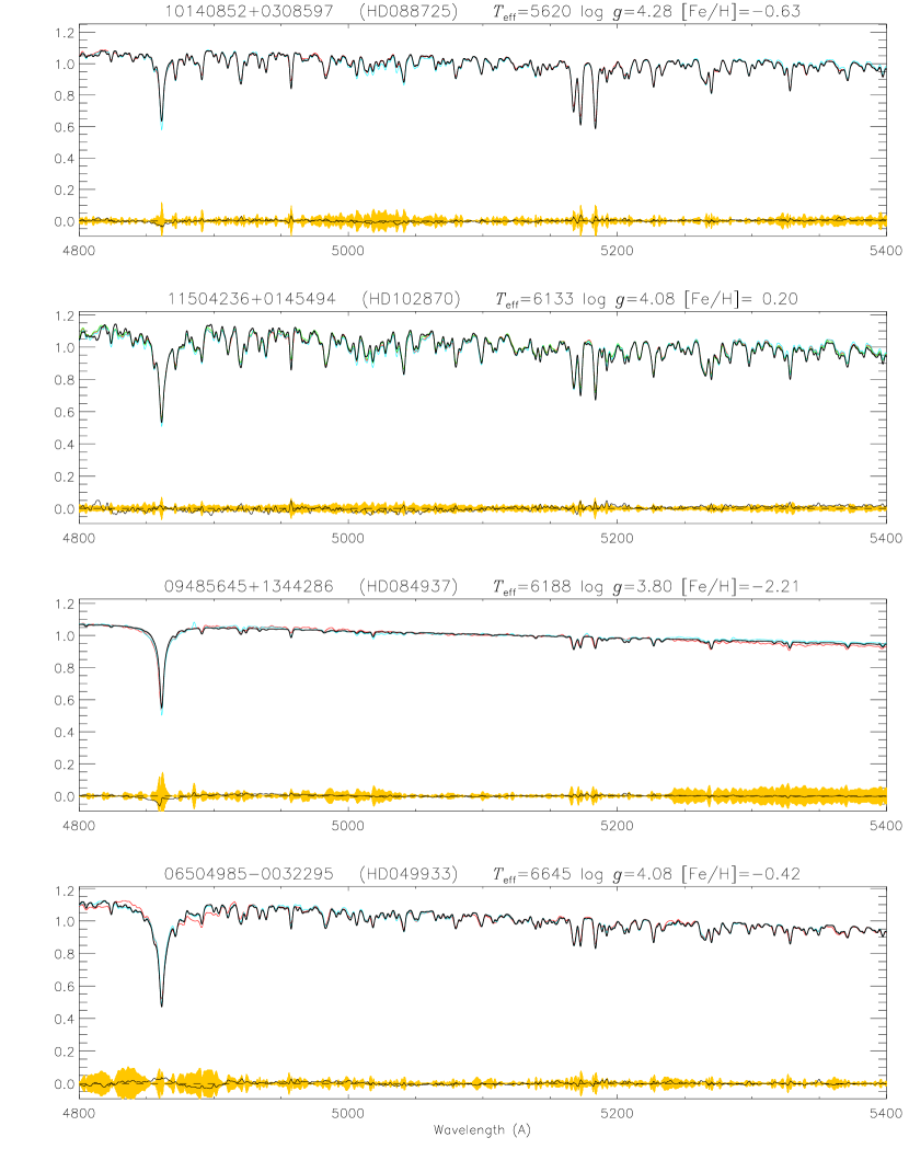
Figure 10: As in Figure 9.

In this Section, the INTRIGOSS FSPs are compared to observed flux calibrated spectra. A search for stars of our UVES-U580 sample within the ELODIE (Prugniel & Soubiran, 2001; Prugniel et al., 2007), INDO–U.S. (Valdes et al., 2004), and MILES (Sánchez-Blázquez et al., 2006) SED libraries provided a list of about 20 stars in common. Eight of them are present in MILES and, at least, in one other SED library and can be used to check the predictions of INTRIGOSS as far as the FSPs are concerned. We chose MILES as the reference SED source because it is one of the most used standard empirical library for stellar population models (see for example Vazdekis et al., 2015). Since only relative fluxes are, in general, needed for this kind of studies we did not attempt to use absolute fluxes but we scaled the observed stellar SEDs and the corresponding synthetic spectra computed using the nominal GES atmospheric parameter values and the individual element abundances of each star (hereafter n_FSPs) according to their median flux value. In Figures 9 and 10 we plot the scaled n_FSPs and observed SEDs together with the residuals obtained after computing the average of the available SEDs, i.e. $<$SED$>$-n_FSP, and the $3\sigma<$SED$>$ uncertainties. These two figures indicate that the n_FSPs for the stars at $T_{\rm eff}<5300$ K reproduce, without any systematic trend, the mean observed SEDs within $\sim 3$%, while for higher $T_{\rm eff}$s the agreement is within 1%. We also remark, by looking at Figures 9 and 10, the absence of the excessive opacity near 5200 Å found by C14 in her synthetic spectra (see their Figure 10). We can conclude that the n_FSPs of the stars in Figures 9 and 10 accurately predict the observed SEDs. Unfortunately, the small number of UVES-U580 stars with accurate observed SEDs does not allow us to check in details, through a complete coverage and a fine sampling, the accuracy of FPSs over the whole extension of INTRIGOSS library in the atmospheric parameter space. Therefore, in next Section we will use, instead of SEDs, a different approach based on the comparison of spectral feature indices.

3.2.2 Comparison of observed and synthetic Mg₁, Mg₂, and Mgb Lick/SDSS indices

For a long time (and still now), several spectroscopic analyses of stellar populations have relied on the Lick/IDS system of indices (Gorgas et al., 1993; Worthey et al., 1994; Worthey & Ottaviani, 1997; Thomas, Maraston & Korn, 2004; Korn, Maraston & Thomas, 2005; Worthey, Danilet & Faber, 2014). More recently, several authors introduced new Lick-like systems (see for example Kim et al., 2016) to avoid the possible uncertainties associated with the response curve of the original Lick/IDS spectrograph and/or any potential loss of information that would occur in degrading spectra obtained from current surveys at medium resolution (e.g. R$\sim$1800) like the Sloan Digital Sky Survey, SDSS, (York et al., 2000) or the Large Sky Area Multi–Object Fiber Spectroscopic Telescope survey, LAMOST,) to match the low resolution (R$\sim$630) of the original Lick/IDS system. One of these Lick-like systems is the Lick/SDSS (Franchini et al., 2010) which was built from observed energy distributions, SEDs, at R=1800 and which is not affected by any particular instrumental signature. The Lick/SDSS indices are computed by integrating the spectrum in central bandpasses covering prominent stellar features after normalization to a pseudo-continuum defined via two bracketing blue and red side bands, and are, therefore, not very sensitive to small inaccuracies in the flux spectra calibration. Nevertheless, since the three bandpasses cover, in some cases, relatively large wavelength ranges, some indices are sensitive not only to the main absorption feature they were designed to measure, but also to the overall line blanketing present in the spectra. It is therefore possible to use them to check the accuracy and completeness of the atomic, molecular, and predicted lines used to compute the FSPs. In fact, if it turns out that the FSPs are able to accurately predict the observed indices, then the accuracy of the atomic and molecular absorption caused by the atmospheric models used to derive them, and therefore of the FSPs themselves, would be substantiated. In the following we will use the comparison between observational and synthetic Lick/SDSS indices as a method to evaluate the validity of the FSPs over the full atmospheric parameter space covered by the UVES-U580 stars. In particular, we chose the Mg₁, Mg₂, and Mgb indices which are characterized by quite extended bandpasses falling in the wavelength region covered by our synthetic spectra. First we computed the observational indices, hereafter UVES-U580 indices, for each of the 2212 stars of the UVES-U580 sample, after removing from the observed (stacked) UVES-U580 spectrum, degraded at $R=$1800, the instrumental signature by means of the corresponding n_FSP. Then, we computed the corresponding synthetic indices from INTRIGOSS FSPs and from the spectra libraries listed in Section 3.1 with the same interpolation adopted in Section 3.1. Unfortunately, the GES_Grid, and B17 libraries contains only normalized spectra and cannot be used to compute Lick/SDSS indices. Therefore, we were able to compute the following synthetic indices:

• n_FSP indices obtained from the above-defined n_FSPs;

• Interp_FSP_α indices obtained from the spectra computed by interpolating INTRIGOSS FSPs at the stellar $T_{\rm eff}$, log $g$, [Fe/H], $\xi$, and $<$[$\alpha$/Fe]$>$;

• Interp_FSP_Mg indices obtained from the spectra computed by interpolating INTRIGOSS FSPs at the stellar [Mg/Fe] abundance ratio instead of at $<$[$\alpha$/Fe]$>$;

• Interp_PHOENIX indices obtained from the spectra computed by interpolating the flux calibrated PHOENIX spectra at the stellar $T_{\rm eff}$, log $g$, [Fe/H], and $<$[$\alpha$/Fe]$>$;

• Interp_C14 indices obtained from the spectra computed by interpolating the flux calibrated C14 spectra at the stellar $T_{\rm eff}$, log $g$, [Fe/H], and $<$[$\alpha$/Fe]$>$.

• Interp_AMBRE indices obtained from the spectra computed by interpolating the flux calibrated AMBRE spectra at the stellar $T_{\rm eff}$, log $g$, [Fe/H], and $<$[$\alpha$/Fe]$>$.

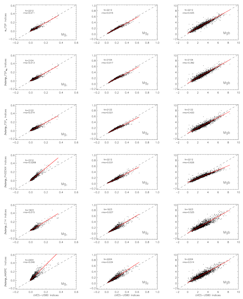
Figure 11: Comparison of synthetic and observational Lick/SDSS indices Mg₁ (left panels), Mg₂ (central panels), and Mgb (right panels). Indices computed from synthetic spectra are plotted versus those measured from UVES-U580 spectra (see text) together with the 45^∘ (dashed) and the regression (red) lines. From top to bottom: n_FSP indices computed from n_FSPs; Interp_FSP_Mg and Interp_FSP_α indices computed from INTRIGOSS; Interp_PHOENIX, Interp_C14, and Interp_AMBRE indices computed from PHOENIX, C14, and AMBRE libraries respectively (see text).

While we were able to compute n_FSPs and, therefore the corresponding n_FSP indices, for all the stars in the UVES-U580 sample, the number of stars for which the interpolation within the spectral grids was possible varies because of the different parameter space coverages. In Figure 11 we plot the synthetic indices versus the UVES-U580 indices. Each panel contains the number of stars (N), the rms of the deviations from the 45^∘ line and the synthetic vs UVES-U580 regression lines. It can be seen that there is a very good agreement between n_FSP indices and UVES-U580 ones indicating that the blanketing of the FSP spectra correctly predict the observed one. The non significant increase of the rms when using Interp_FSP_α and Interp_FSP_Mg indices indicates that spectra computed from individual star models and element abundances provides synthetic indices that are almost equivalent to those obtained by Interp_FSPs. This different result with respect to that one obtained by looking at the $r_{med}$ values (see Section 3.1) could be ascribed to the lower sensitivity of the spectral index comparison with respect to that one performed at each wavelength point.

The panels referring to Interp_PHOENIX, Interp_C14, and Interp_AMBRE indices show a larger rms and/or some systematic trend. The deviations of the Mg₁, Mg₂ indices derived from PHOENIX and AMBRE spectra from the 45^∘ line indicates significant differences in the blanketing predicted by these spectra. In the case of the indices derived from C14 spectra the deviations are smaller and the increase of rms is present only in Mg₂ and Mgb. It is worthwhile to recall that the comparison with the UVES-U580 indices is, in this case, limited to stars with $-1.0<[Fe/H]<0.2$ dex due to the absence of super-metal rich spectra in the C14 library. The small systematic deviations may indicate that C14 has, on average, more accurate line lists than PHOENIX and that the increase in rms with respect to the upper panels may be due to the different treatment of the PLs.

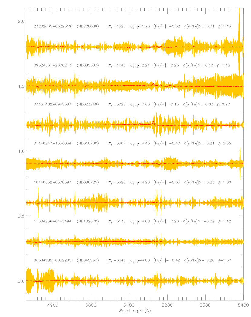
Figure 12: Comparison between the 3$\sigma$ of the $<$SEDs$>$ (yellow area) and the differences between the intra-mesh and the interpolated INTRIGOSS FSPs (red lines) for seven of the stars discussed in Section 3.2. Horizontal dashed black lines represent the zero levels after vertical shifts applied to better visualize all the stars in the same plot.

Concerning the errors introduced by our interpolation procedure, we confirm the results already obtained in Section 3.1 also for FSPs. In addition, we computed intra-mesh FSPs for the seven stars in Figures 9 and 10 for which we were able to compute interpolated INTRIGOSS FSPs. Then, we compare the $3\sigma$ uncertainties of the $<$SED$>$ of these stars with the differences between the intra-mesh and the interpolated INTRIGOSS FSPs. Figure 12 shows that the interpolation procedure introduces inaccuracies in the spectra (red lines) which are well below the SEDs uncertainties (yellow areas).

Eventually, we compared the Interp_FSP_α indices with those computed by using the 50 intra-mesh FSPs to estimate the effect of the interpolation on the computation of the indices and we did not find any systematic trend in the differences. The use of the interpolated spectra instead of the intra-mesh ones introduces an rms scatter which is one order of magnitude smaller than those reported in the first row of Figure 11 showing that the interpolation error on the indices does not undermine the above-given discussion about the indices computed with the different spectral libraries.

In conclusion, the comparison of observational and synthetic Mg₁, Mg₂, and Mgb Lick/SDSS indices indicates that the INTRIGOSS FSPs predict well the observed blanketing thus suggesting that this library can provide accurate synthetic SEDs not only for the stars discussed in Section 3.2.1 but also for all of those in the UVES-U580 sample.

4 Data products

The INTRIGOSS spectral library and the linelist used to compute the synthetic spectra are available on the website http://archives.ia2.inaf.it/intrigoss together with auxiliary data.

The synthetic spectra are computed from 4830 to 5400 Å at wavelength sampling $\Delta\lambda=0.01$ Å, rotational velocity of 0 km s^-1 , and, in order to be consistent with the ATLAS12 models, with microturbulent velocities $\xi$ = 1 and 2 km s^-1 leading to a final total number of 7616 NSPs and 7616 FSPs.

The gaps in the final grid are due to the absence of converging ATLAS12 atmosphere models for log $g=0.5$ dex and $T_{\rm eff}\geq 6250$ K. In order to keep the grid homogeneous, we decided to avoid any patches based on, for example, the use of ATLAS9 atmosphere models. Work is in progress to attain convergence of ATLAS12 code at relatively high temperatures and low surface gravities.

The INTRIGOSS spectra are provided in FITS binary table format and can be downloaded by selecting:

• the type of spectra: NSP, FSP, or both;

• a range in $T_{\rm eff}$ and/or log $g$ and/or [Fe/H] and/or [$\alpha$/Fe] and/or $\xi$, or the whole library (15232 spectra);

The following auxiliary data are also available from links given in the http://archives.ia2.inaf.it/intrigoss-details web-page:

• A FITS binary table with the line list of atomic and molecular transitions used in computing INTRIGOSS synthetic spectra. The table contains 1427628 entries in the format of the linelist file used by SPECTRUM code (see Section 3.3.1 and 3.6 of Documentation for SPECTRUM Gray & Corbally, 1994), i.e, for each line we list:

  • WAVELENGTH: wavelength in Å;

  • ELEM_ION: element and ion identifier, e.g. 26.1 for FeII;

  • ISOTOPE: mass number of isotope (the 0 code corresponds to entries representing all possible isotopes for that species taken together);

  • ELOW: energy of the lower state in cm^-1;

  • EHIGH: energy of the upper state in cm^-1; this entry is sometimes used to encode the molecular band information since only ELOW is used in molecular calculation;

  • LOG_GF: the logarithm of the product of the statistical weight of the lower level and the oscillator strength for the transition;

  • FUDGE: a fudge factor to adjust the line broadening;

  • TRANSITION_TYPE: the type of transition;

  • REFERENCE: The sub-set of lines with derived astrophysical gf values are indicated as FRA18 and FRA18_P for laboratory and predicted lines, respectively.

• A FITS binary image with the very high SNR ($\sim$4000) observed solar spectrum described in Section 2.2.1 and used to derive astrophysical log(gf) values;

• A set of 100 FITS binary tables with synthetic spectra (50 NSPs and 50 FSPs) computed at 50 representative intra-mesh positions. These spectra are used in Section 3.1 to test the errors arising from our interpolation procedure of the INTRIGOSS spectra.

5 Summary

In this paper we present a new high resolution synthetic spectral library, INTRIGOSS, which covers the parameter space range of F, G, and K stars. INTRIGOSS is based on atmosphere models computed with ATLAS12 which allowed us to specify each individual element abundance. The normalized (NSP) and surface flux (FSP) spectra, in the 4830-5400 Å  wavelength range, were computed in a fully consistent mode by means of SPECTRUM v2.76f code using the detailed solar composition by Grevesse et al. (2007) and varying it by adopting different [$\alpha$/Fe] abundance ratios. Particular attention was devoted to derive astrophysical gf-values by comparing synthetic prediction with a very high SNR solar spectrum and good SNR UVES-U580 spectra of cool giants. The validity of the obtained spectra and, in particular, of the used astrophysical gf-values, was assessed by using as reference more than 2000 stars with homogeneously and accurately derived atmospheric parameter values and detailed chemical compositions.

The greater accuracy of INTRIGOSS NSPs with respect to other publicly available stellar libraries, i.e. AMBRE, GES_Grid, PHOENIX, C14, and B17, in reproducing the observed spectra was shown by computing a figure of merit, $r_{med}$, to evaluate the consistency of the prediction of different libraries with respect to the spectra of the UVES-U580 sample stars.

As far as the FSPs are concerned, the comparison with SEDs derived from ELODIE, INDO–U.S., and MILES libraries showed that they reproduce the observed flux distributions within a few percent without any systematic trend. A check on the predicted blanketing of FSPs and, therefore, on the adopted line lists (including the treatment of the Predicted Lines) based on Lick/SDSS indices comparison confirmed the reliability of INTRIGOSS surface flux spectra and their ability to better reproduce the observational index values with respect to PHOENIX, AMBRE and C14 libraries.

The results of the validity checks on both INTRIGOSS normalized (NSP) and surface flux spectra (FSP) make us confident that the presented spectral library, which is available on the web together with the adopted line list and the observed solar spectrum (see Section 4), will provide to the astronomical community a valuable tool for both stellar atmosphere parameter determinations and stellar population studies.

Figure 5: Distribution of n_$r^{\rm i}_{med}$ obtained by using the nominal atmospheric parameter values in computing the synthetic spectra (top panel); trend of the median values of the n_$r^{\rm i}_{med}$ computed in overlapped bins containing 51 stars each vs $T_{\rm eff}$, log $g$, and [Fe/H] (second, third, and fourth panel respectively from top to bottom).

Appendix A Unidentified spectral features

Together with the accurate determination of astrophysical log(gf) values, the analysis of the Solar spectrum and of the GES spectra of the five giant stars in Table 1 allows us to determine where the adopted line list is missing features. To construct the list of these unidentified features we computed the difference between the observed and synthetic spectrum of the Sun and of the five giants and the corresponding standard deviations ($\sigma{{}_{\rm Sun}}$, $\sigma_{\rm i}$). Then, we run the LineSearcher code, which is a derivation from the ARES code (Sousa et al., 2015), using as input the six files of the differences and we obtained for all the absorption features in the differences, i.e. those below zero, their center wavelength and depth. Eventually, we extracted from the solar LineSearcher output all the features which have a depth larger than 2$\sigma{{}_{\rm Sun}}$ while a 3$\sigma_{\rm i}$ threshold was used in the case of the five giants, due to the lower resolution and SNR of their spectra. At the end we checked if the so selected features were present in more than one spectra but with smaller depths. Table 4 lists the wavelength of each unidentified feature together with its depth in all the stars in which it is detectable while Table 5 shows the total number of detected unidentified features in each star spectrum (column 2), and the number of those with depth between 2$\sigma$ and 3$\sigma$ (column 3) and larger than 3$\sigma$ (column 4).

Table 4: Unidentified spectral lines

	SUN	00241708-7206106	00251219-7208053	00240054-7208550	02561410-0029286	03173493-0022132
$\sigma$:	0.03	0.04	0.04	0.04	0.03	0.03
Wavelength [$\AA$]	Depth	Depth	Depth	Depth	Depth	Depth
4834.60	0.08	0.12	0.04	0.10	0.05	–
4844.19	–	–	–	0.14	–	–
4855.20	0.05	–	0.17	–	–	–
4858.14	0.11	–	0.08	–	0.06	–
4861.95	0.08	0.20	0.21	0.18	0.15	0.11
4866.72	0.04	–	–	–	–	0.09
4880.97	0.06	0.08	–	0.09	0.07	0.04
4884.94	0.13	0.16	0.21	0.15	0.11	0.10
4906.80	0.07	–	0.08	0.05	–	0.03
4916.23	0.07	0.03	0.06	0.03	–	–
4916.49	0.14	0.04	0.10	0.06	–	–
4921.85	–	–	–	–	–	0.14
4922.81	0.07	–	–	–	–	–
4927.88	0.59	0.40	0.43	0.42	0.33	0.35
4934.20	–	–	–	0.22	–	–
4937.09	0.07	–	–	–	–	–
4940.06	0.16	0.10	0.10	0.09	0.04	0.06
4940.50	0.08	–	–	–	–	–
4944.29	0.11	–	–	–	–	0.03
4948.33	0.07	–	0.09	–	–	–
4954.60	–	–	–	–	–	0.10
4961.05	0.13	0.10	0.15	0.10	0.07	0.07
4964.14	0.08	–	–	–	–	–
4966.29	0.09	0.09	0.11	0.08	0.08	0.04
4971.35	0.51	0.29	0.31	0.32	0.27	0.30
4990.45	0.27	0.18	0.22	0.19	0.16	0.13
5013.93	0.17	0.13	0.09	0.11	0.08	0.08
5016.89	0.44	0.28	0.27	0.27	0.22	0.22
5031.18	0.06	–	0.07	0.06	–	–
5036.28	0.43	0.30	0.31	0.29	0.22	0.22
5041.34	0.07	0.09	0.07	0.06	0.05	0.07
5041.44	0.08	0.11	0.09	0.09	0.05	0.07
5088.16	0.18	0.10	0.11	0.10	0.06	0.09
5092.29	0.07	–	0.04	0.04	0.04	0.05
5097.49	0.38	0.24	0.24	0.23	0.19	0.18
5136.27	0.08	0.05	0.08	–	–	–
5140.82	0.14	0.08	0.09	0.09	0.04	0.05
5156.66	0.13	–	0.06	0.06	0.05	0.07
5157.21	0.08	–	–	–	–	–
5169.30	0.14	0.08	0.08	0.08	0.07	0.06
5170.77	0.29	0.10	0.10	0.10	0.09	0.08
5179.78	0.03	–	–	–	–	0.10
5181.32	0.16	–	–	–	–	–
5212.22	0.08	–	0.06	–	–	–
5214.61	0.11	0.05	0.03	0.04	0.05	0.03
5215.57	0.14	–	–	–	–	–
5217.89	0.13	–	–	–	–	–
5221.03	0.20	0.12	0.12	0.09	0.09	0.10
5221.75	0.12	0.04	–	0.06	–	0.03
5225.81	0.14	–	–	–	–	–
5226.13	0.08	0.05	0.02	0.04	0.03	–
5228.10	0.12	–	–	–	–	–
5242.06	0.15	0.06	–	–	–	0.06
5243.18	0.10	0.06	–	–	–	0.03
5248.98	0.08	0.09	0.10	0.08	0.07	0.05
5255.70	0.07	0.08	0.10	0.12	0.05	0.06
5263.77	0.07	0.09	–	–	–	–
5272.00	0.09	–	–	–	–	–
5274.53	0.10	0.06	0.05	0.06	–	0.04
5275.13	0.22	–	–	–	–	–
5276.17	0.07	–	0.08	0.08	–	0.06
5278.78	0.08	–	–	–	–	–
5281.32	0.10	–	–	–	–	–
5284.34	–	–	0.21	0.16	–	–
5298.51	0.11	–	–	–	–	–
5299.97	0.11	–	–	–	–	–
5303.84	0.06	–	–	–	–	–
5314.92	0.07	–	–	0.03	–	–
5341.15	0.27	0.30	0.25	0.29	0.23	0.22
5370.30	0.06	0.04	0.06	–	–	0.04
5389.85	0.09	–	0.08	–	–	–
5390.53	0.19	–	0.05	0.05	0.04	0.06

Note. — Depth values larger than 3$\sigma$ are in bold

Table 5: Number of unidentified features

Star	Ntot	N2σ-3σ	N>3σ
Sun	67	25	35
00241708-7206106	36	11	10
00251219-7208053	42	12	12
00240054-7208550	40	11	12
02561410-0029286	30	8	9
03173493-0022132	39	10	17

References

- Anders & Grevesse (1989) Anders,E. & Grevesse, N. 1989, Geochim. Cosmochim. Acta, 53, 197
- Brahm et al. (2017) Brahm, R., Jordán, A.; Hartman, J., & Bakos, G. 2017, MNRAS, 467, 971 (B17)
- Castelli (2005) Castelli, F., 2005, Mem. Soc. Astron. Ital. Suppl., 8, 34
- Castelli & Kurucz (2003) Castelli, F., Kurucz, R. L. 2003, in IAU Symp. 210, Modelling of Stellar Atmosphere, ed. N. E. Piskunov,W.W.Weiss, & D. F. Gray (San Francisco, CA: ASP), A20
- Coelho et al. (2005) Coelho P., Barbuy B., Meléndez J., et al. 2005, A&A, 443, 735 (C05)
- Coelho (2014) Coelho, P. R. T. 2014, MNRAS, 440, 1027 (C14)
- Dekker et al. (2000) Dekker H., D’Odorico S., Kaufer A., Delabre B., Kotzlowski H., in Iye M., Moorwood A. F., eds, Proc. SPIE Conf. Ser. Vol. 4008, Optical and IR Telescope Instrumentation and Detectors. SPIE, Bellingham, p. 534
- de Laverny et al. (2012) de Laverny, P., Recio-Blanco, A., Worley, C. C., Plez, B. 2012, A&A, 544, A126 (AMBRE)
- De Silva et al. (2015) De Silva, G. et al. 2015, MNRAS, 449, 2604
- Franchini et al. (2010) Franchini M., Morossi C., Di Marcantonio P., Malagnini M. L., Chavez M., 2010, ApJ, 719, 240
- García Pérez, et al. (2015) García Pérez, A. E., et al. 2015, AJ, 151, 144
- Gilmore et al. (2012) Gilmore, G. et al. 2012, The Messenger, 147, 25
- Gonneau et al. (2016) Gonneau, A. et al. 2016, A&A, 589, A36
- Gorgas et al. (1993) Gorgas, J. et al. 1993, ApJS, 86, 153
- Gray & Corbally (1994) Gray, R. O., & Corbally, D. J. L. I. 1994, AJ, 107, 742
- Grevesse et al. (2007) Grevesse, N., Asplund, M., Sauval, A. J. 2007, Space Sci. Rev., 130, 105
- Gustafsson et al. (2008) Gustafsson, B., Edvardsson, B., Eriksson, K., et al. 2008, A&A, 486, 951
- Hauschildt & Baron (1999) Hauschildt, P. H., & Baron, E. 1999, J. Computat. Appl. Math., 109, 41
- Hubeny (1988) Hubeny, I. 1988 Computer Physics Communications, Volume 52, Issue 1, p. 103-132
- Husser et al. (2013) Husser, T.-O., Wende-von Berg, S., Dreizler, S., et al. 2013, A&A553, A6 (PHOENIX)
- Jacoby, Hunter, & Christian (1984) Jacoby, G. H.; Hunter, D. A.; Christian, C. A. 1984, ApJS, 56, 257
- Jofré et al. (2015) Jofré et al. 2015, A&A, 582, A81
- Kim et al. (2016) Kim, H. et al. 2016, AJSS, 227, 24
- Korn, Maraston & Thomas (2005) Korn A., Maraston C., Thomas D. 2005, A&A, 438, 685
- Kos et al. (2017) Kos, J., et al. 2017, MNRAS, 464, 1259
- Kurucz (1979) Kurucz, R. L. 1979, ApJS, 40, 1
- Kurucz (2005a) Kurucz, R. L. 2005a, Mem. Soc. Astron. Ital. Suppl., 8, 14
- Kurucz (2005b) Kurucz, R. L. 2005b, Mem. Soc. Astron. Ital. Suppl., 8, 76
- Kurucz (2014) Kurucz, R. L. 2014, in “Determination of Atmospheric Parameters of B-, A-, F- and G-Type Stars.” Series: GeoPlanet: Earth and Planetary Sciences, ISBN: 978-3-319-06955-5. Springer International Publishing (Cham), Edited by Ewa Niemczura, Barry Smalley and Wojtek Pych, pp. 63-73
- Leitherer et al. (1996) Leitherer, C. Alloin, D., Alvensleben, U. F.-v, et al. 1996, PASP, 108, 996
- Lobel (2011) Lobel, A.2011, CaJPh, 89,395
- Magrini et al. (2017) Magrini, L., Randich, S., Kordopatis, G. et al. 2017, A&A, 603A, 2
- Majewski et al. (2017) Majewski, Steven R., Schiavon, Ricardo P., Frinchaboy, Peter M., el al. 2017, AJ, 154, 94
- Mészáros & Allende Prieto (2013) Mészáros, Sz. & Allende Prieto, C. 2013, MNRAS, 430, 3285
- Molaro et al. (2013) Molaro, P., Monaco, L., Barbieri, M., Zaggia, S. 2013, MNRAS, 429, 79
- Moultaka et al. (2004) Moultaka, J., Ilovaisky, S. A., Prugniel, P., Soubiran, C. 2004, PASP, 116, 693 (ELODIE)
- Munari et al. (2005) Munari, U., Sordo, R., Castelli, F., & Zwitter, T. 2005, A&A, 442, 1127
- Partridge & Schwenke (1997) Partridge, H., & Schwenke, D. W. 1997, J. Chem. Phys., 106, 4618
- Prugniel & Soubiran (2001) Prougniel, Ph. & Soubiran, C. 2001, A&A, 369, 1048
- Prugniel et al. (2007) Prugniel,Ph et al. 2007, arXiv:astro-ph/0703658
- Randich & Gilmore (2013) Randich, S., Gilmore, G., Gaia-ESO Consortium 2013, The Messenger, 154,47
- Sacco et al. (2014) Sacco G. G. et al. 2014, A&A, 565,513
- Sánchez-Blázquez et al. (2006) Sánchez-Blázquez et al. 2006, MNRAS, 371, 703 (MILES)
- Schwenke (1998) Schwenke, D. W. 1998, Faraday Discuss., 109, 321
- Smiljanic et al. (2014) Smiljanic R. et al. 2014, A&A, 570, A122
- Sousa et al. (2015) Sousa, S. G. et al. 20145, A&A, 577, A67
- Swan (1957) Swan, W. 1857, Transactions of the Royal Society of Edinburgh, 21, 411
- Thomas, Maraston & Korn (2004) Thomas D., Maraston C., Korn A. 2004, MNRAS, 351, L19
- Valdes et al. (2004) Valdes, F. et al. 2004, ApJS, 152, 251 (INDO-U.S.)
- Vazdekis et al. (2015) Vazdekis, A. et al. 2004, MNRAS, 449, 1177 (INDO-U.S.)
- Weck et al. (2003) Weck, P. F. et al. 2003, ApJ, 582, 1059
- Worley et al. (2016) Worley, C. C. et al. 2016, A&A, 591, A81
- Worthey et al. (1994) Worthey, G. et al. 1994, ApJS, 94, 687
- Worthey & Ottaviani (1997) Worthey G. & Ottaviani D. L., 1997, ApJS, 111, 377
- Worthey, Danilet & Faber (2014) Worthey, G., Danilet, A. B., Faber, S. M., 2014, A&A561, A36
- Yanny et al. (2009) Yanny, B., Rockosi, C., Newberg, H. J., et al. 2009, AJ, 137, 4377
- York et al. (2000) York, D. G. et al. 2000,AJ, 120, 1579