Abstract

We extend the so-called singlet doublet dark matter model, where the dark matter is an admixture of a Standard Model singlet and a pair of electroweak doublet fermions, by a singlet scalar field. The new portal coupling of it with the dark sector not only contributes to the dark matter phenomenology (involving relic density and direct detection limits), but also becomes important for generation of dark matter mass through its vacuum expectation value. While the presence of dark sector fermions affects the stability of the electroweak vacuum adversely, we find this additional singlet is capable of making the electroweak vacuum absolutely stable upto the Planck scale. A combined study of dark matter phenomenology and Higgs vacuum stability issue reflects that the scalar sector mixing angle can be significantly constrained in this scenario.

1 Introduction

Although the discovery of the 125 GeV Higgs boson at Large Hadron Collider (LHC) [1, 2] undoubtedly marks the ultimate success of the Standard Model (SM), there are issues in particle physics and cosmology, supported by observations, which can not be explained in the SM framework. For example, SM justifies only 5% of the total matter content of the Universe preferably known as visible matter. Compelling evidences from astrophysical and cosmological observations of cosmic microwave background radiation (CMBR), spiral galaxy rotation curve, colliding clusters etc. indicate the presence of unknown matter, called dark matter (DM) which constitutes 25% of the Universe. There are some other theoretical issues for which SM can not provide clear answer. In particular, it is well known that the Higgs quartic coupling ($\lambda_{H}$) turns negative at energy scale $\Lambda_{I}^{\textrm{SM}}\sim 10^{10}$ GeV [3, 4, 5, 6, 7] (with $m_{t}=173.2$ GeV [8]) leading to a possible instability of the electroweak (EW) minimum[9]. However the conclusion crucially depends on precise value of the top quark and Higgs mass. In presence of a deeper minimum compared to the EW one, question will also arise why the Universe has chosen the EW vacuum over the global minimum [10, 11, 15, 12, 13, 14].

In order to circumvent these shortcomings of the SM, one has to introduce new physics beyond the Standard Model. In an earlier attempt [16], the SM is extended with two SM singlet scalars, one is with zero and other has non-zero vacuum expectation value (vev). It is shown in [16] that while the singlet scalar with zero vev plays the role of the DM, the other scalar with non-zero vev mixes with SM Higgs (Higgs portal) and affect the dark matter phenomenology in such a way that the scalar DM having mass $\sim 200$ GeV and onward can satisfy the relic density and direct search constraints from LUX[17], XENON-1T[18], Panda 2018[19] and XENON-nT[20]. On the other hand, it turns out that the interaction of the scalar fields with SM Higgs can modify the instability scale ($\Lambda_{I}$) to a value larger than $\Lambda_{I}^{\textrm{SM}}$ by several order of magnitude. In fact the scalar with non-zero vacuum expectation value having mass smaller than $\Lambda_{I}^{\textrm{SM}}$ can indeed make the electroweak vacuum absolutely stable [16] with the help of threshold effect[21, 22, 23]. Other works involving DM and EW vacuum stability can be found in [24, 25, 26, 27, 28, 32, 33, 29, 30, 31]. The extra scalar field(s) could also be connected to several other unresolved physics of the Universe involving inflation[34, 35, 36] or neutrinos[37, 38, 39, 40, 41, 42, 43] etc.

In this work we consider the singlet doublet dark matter (SDDM) scenario and explore how it can be extended minimally (if required) so as to achieve the EW vacuum stability till $M_{P}$. In a typical SDDM model [44, 45, 46, 47, 48, 49, 50, 51, 52, 53, 54, 55, 56, 57, 58, 59], the dark sector is made up with two Weyl fermion doublets and one Weyl singlet fermion. The Yukawa interactions of them with SM Higgs result three neutral fermion states, the lightest of which becomes a viable candidate for DM provided the stability is guaranteed by some symmetry argument. Unlike Higgs portal dark matter models, singlet doublet dark matter scenario directly couples the mass and dynamics of dark sector with the SM gauge sector. This is analogous to the case of supersymmetric extensions[60] where the supersymmetry breaking scale provides mass of dark matter [50]. Singlet doublet dark matter models also induce considerable co-annihilation effect which is absent in usual Higgs portal DM scenarios. Another interesting feature of SDDM model is related to evading the direct detection bound with some specified “blind spots” of the model [50].

The SDDM carries different phenomenology from the usual extension of dark sector with vector-like fermion doublet and singlet [61, 62, 63, 64, 66, 65] due to the involvement of three neutral Majorana fermions in SDDM as compared to two vector like neutral fermions in [61, 62, 63, 64, 66]. In case of vector like singlet doublet models, it is possible to have interaction with $Z$ boson which can enhance the spin independent dark matter nucleon cross-section considerably. On the other hand, in case of SDDM, such interaction is suppressed [50]. Although in SDDM, spin dependent interaction (i.e. axial vector interaction) survives, the bounds on spin dependent dark matter nucleon cross-section[67] is not that stringent compared to spin independent limits and hence remain well below the projected upper limits. Therefore it relaxes the bounds on model parameters in the singlet doublet model allowing the model to encompass a large range of parameter space.

Although the SDDM has many promising features as mentioned above, it also has some serious issues with the Higgs vacuum stability. The model involves new fermions, which can affect the running of Higgs quartic coupling leading to instability at high energy scale [68]. In an attempt to solve the Higgs vacuum stability where the DM is part of the SDDM model, we propose an extension of the SDDM with a SM singlet scalar. We employ a $Z_{4}$ symmetry under which all the beyond SM fields carry non-trivial charges while SM fields are not transforming. The salient features of our model are the followings:

• There exists a coupling between the additional scalar and the singlet Weyl fermion which eventually contributes to the mass matrix involving three neutral Weyl fermions. After the SM Higgs doublet and the scalar get vevs, mixing between neutral singlet fermion and doublet Weyl fermions occur and the lightest neutral fermion can serve as a stable Majorana dark matter protected by the residual $Z_{2}$ symmetry. In this way, the vev of the additional scalar contributes to the mass of the DM as well as the mixing.

• Due to the mixing between this new scalar and the SM Higgs doublet, two physical Higgses will result in this set-up. One of these would be identified with the Higgs discovered at LHC. This set-up therefore introduces a rich DM phenomenology (and different as compared to usual SDDM model) as the second Higgs would also contribute to DM annihilation and the direct detection cross-section.

• The presence of the singlet scalar with non-zero vev helps in achieving the absolute stability of the EW vacuum. Here the mixing between singlet doublet scalars (we call it scalar mixing) plays an important role. Hence the combined analysis of DM phenomenology (where this scalar mixing also participates) and vacuum stability results in constraining this scalar mixing at a level which is even stronger than the existing limits on it from experiments.

The paper is organized as follows. In Sec. 2, we describe the singlet scalar extended SDDM model. Various theoretical and observational limits on the specified model are presented in Sec. 3. In the next section, we present our strategy, the related expressions including Feynman diagrams for studying dark matter phenomenology of this model. The discussion on the allowed parameter space of the model in terms of satisfying the DM relic density and direct detection limits are also mentioned in this Sec. 4. In Sec. 5, the strategy to achieve vacuum stability of the scalar enhanced singlet doublet model is presented. In Sec. 6, we elaborate on how to constrain parameters of the model while having a successful DM candidate with absolute vacuum stability within the framework. Finally the work is concluded with conclusive remarks in Sec. 7.

2 The Model

Like the usual singlet doublet dark matter model[45, 46, 47, 48], here also we extend the SM framework by introducing two doublet Weyl fermions, $\psi_{D_{1}},\psi_{D_{2}}$ and a singlet Weyl fermion field $\psi_{S}$. The doublets are carrying equal and opposite hypercharges ($Y=\frac{1}{2}(-\frac{1}{2})$ for $\psi_{{D_{1}}(D_{2})}$) as required from gauge anomaly cancellation. Additionally the scalar sector is extended by including a SM real singlet scalar field, $\phi$. There exists a $Z_{4}$ symmetry, under which only these additional fields are charged which are tabulated in Table 1. The purpose of introducing this $Z_{4}$ is two fold: firstly it avoids a bare mass term for the $\psi_{S}$ field. Secondly, although the $Z_{4}$ is broken by the vev of the $\phi$ field, there prevails a residual $Z_{2}$ under which all the extra fermions are odd. Hence the lightest combination of them is essentially stable. Note that with this construction, not only the DM mass involves vev of $\phi$ but also the dark matter phenomenology becomes rich due to the involvement of two physical Higgs (as a result of mixing between $\phi$ and the SM Higgs doublet $H$). Apart from these, $\phi$ is also playing a crucial role in achieving electroweak vacuum stability. The purpose of $\phi$ will be unfolded as we proceed. For the moment, we split our discussion into two parts first as extended fermion and next as scalar sectors of the model.

Symmetry	$\psi_{D_{1}}$	$\psi_{D_{2}}$	$\psi_{S}$	$\phi$
$Z_{4}$	-i	i	i	-1

Table 1: Particle multiplets and their transformation properties under $Z_{4}$ symmetry.

2.1 Extended fermion sector

The dark sector fermions $\psi_{D_{1}},\psi_{D_{2}}$ and $\psi_{S}$ are represented as,

$$\psi_{D_{1}}=\left(\begin{array}[]{c}\psi_{1}^{0}\\ \psi_{1}^{-}\end{array}\right)\leavevmode\nobreak\ \leavevmode\nobreak\ :[2,\frac{1}{2}]\,\,,\leavevmode\nobreak\ \leavevmode\nobreak\ \leavevmode\nobreak\ \leavevmode\nobreak\ \leavevmode\nobreak\ \psi_{D_{2}}=\left(\begin{array}[]{c}\psi_{2}^{+}\\ \psi_{2}^{0}\end{array}\right)\leavevmode\nobreak\ \leavevmode\nobreak\ :[2,-\frac{1}{2}]\,\,,\leavevmode\nobreak\ \leavevmode\nobreak\ \leavevmode\nobreak\ \leavevmode\nobreak\ \leavevmode\nobreak\ \psi_{S}\leavevmode\nobreak\ \leavevmode\nobreak\ :[1,0]\,\,.$$ (1)

Here field transformation properties under SM ($SU(2)_{L}\times U(1)_{Y}$) are represented within square brackets. The additional fermionic Lagrangian in the present framework is therefore given as

$${\cal L}_{Dark} = i\psi_{D_{1}}^{\dagger}{{\bar{\sigma}}^{\mu}}{D_{\mu}}{\psi_{D_{1}}}+i\psi_{D_{2}}^{\dagger}{{\bar{\sigma}}^{\mu}}{D_{\mu}}{\psi_{D_{2}}}+$$ (2)

$$i\psi_{S}^{\dagger}{{\bar{\sigma}}^{\mu}}{\partial_{\mu}}{\psi_{S}}-({m_{\psi}}\epsilon^{ab}{\psi_{D_{1}a}}{\psi_{D_{2}b}}+\frac{1}{2}c\phi\psi_{S}\psi_{S}+h.c.)\,\,,$$

where $D_{\mu}$ is the gauge covariant derivative in the Standard Model, $D_{\mu}=\partial_{\mu}-igW_{\mu}^{a}\frac{\sigma_{a}}{2}-ig^{\prime}YB_{\mu}$. From Eq.(2) it can be easily observed that after $\phi$ gets a vev, the singlet fermion $\psi_{S}$ in the present model receives a Majorana mass, $m_{\psi_{S}}=c\langle\phi\rangle$.

Apart from the interaction with the singlet scalar $\phi$, the dark sector doublet $\psi_{D_{1}}$ and singlet $\psi_{S}$ can also have Yukawa interactions with the Standard Model Higgs doublet, $H$. This Yukawa interaction term is given as

$$-{{\cal L}_{{\rm{Y}}}}={\lambda}\psi_{S}\psi_{D_{1}}{H}+h.c.\,\,.$$ (3)

Note that due to $Z_{4}$ charge assignment, $\psi_{D_{2}}$ does not have such Yukawa coupling in this present scenario. Once $\phi$ gets a vev $v_{\phi}$ and the electroweak symmetry is broken (with $H$ acquires a vev $v/{\sqrt{2}}$, with $v=246$ GeV), Eq.(3) generates a Dirac mass term for the additional neutral fermions. Hence including Eq.(2) and Eq.(3), the following mass matrix (involving the neutral fermions only) results

$$\mathcal{M} = \left(\begin{array}[]{ccc}m_{\psi_{S}}&\frac{1}{\sqrt{2}}\lambda v&0\\ \frac{1}{\sqrt{2}}\lambda v&0&m_{\psi}\\ 0&m_{\psi}&0\end{array}\right).$$ (7)

The matrix is constructed with the basis $\mathcal{X}^{T}=(\psi_{S},\leavevmode\nobreak\ \psi_{1}^{0},\leavevmode\nobreak\ \psi_{2}^{0})$. On the other hand, the charged components have a Dirac mass term, $m_{\psi}\psi_{1}^{-}\psi_{2}^{+}+h.c.$.

In general the mass matrix $\mathcal{M}$ could be complex. However for simplicity, we consider the parameters $m_{\psi_{S}},\lambda$ and $m_{\psi}$ to be real. By diagonalizing this neutral fermion mass matrix, we obtain $V^{T}\mathcal{M}V=diag(m_{\chi_{1}},m_{\chi_{2}},m_{\chi_{3}})$, where the three physical states $\mathcal{P}^{T}=(\chi_{1},\chi_{2},\chi_{3})$ are related to $\mathcal{X}$ by,

$$\mathcal{X}_{i}=V_{ij}\mathcal{P}_{j},$$ (8)

where $V$ is diagonalizing matrix of $\mathcal{M}$. Then the corresponding real mass eigenvalues obtained at the tree level are given as [47, 69]

$$m_{\chi_{1}} =-\frac{B}{3A}-\frac{2}{3A}\Big{(}\frac{R}{2}\Big{)}^{1/3}\cos\theta_{m}\,,$$ (9)

$$m_{\chi_{2}} =-\frac{B}{3A}+\frac{1}{3A}\Big{(}\frac{R}{2}\Big{)}^{1/3}(\cos\theta_{m}-\sqrt{3}\sin\theta_{m})\,,$$ (10)

$$m_{\chi_{3}} =-\frac{B}{3A}+\frac{1}{3A}\Big{(}\frac{R}{2}\Big{)}^{1/3}(\cos\theta_{m}+\sqrt{3}\sin\theta_{m})\,,$$ (11)

where $A=1,\leavevmode\nobreak\ B=-m_{\psi_{S}},\leavevmode\nobreak\ C=-(m_{\psi}^{2}+\frac{\lambda^{2}v^{2}}{2}),\leavevmode\nobreak\ D=m_{\psi}^{2}m_{\psi_{S}}$ (provided the discriminant ($\Delta$) of $\mathcal{M}$ is positive). Now $R$ and the angle $\theta_{m}$ can be expressed as

$$R=\sqrt{P^{2}+Q^{2}},\leavevmode\nobreak\ \leavevmode\nobreak\ \leavevmode\nobreak\ \leavevmode\nobreak\ \leavevmode\nobreak\ \tan 3\theta_{m}=\frac{Q}{P}\,\,,$$ (12)

where $P=2B^{3}-9ABC+27A^{2}D$ and $Q=3\sqrt{3\Delta}A$, $\Delta=18ABCD-4B^{3}D+B^{2}C^{2}-4AC^{3}-27A^{2}D^{2}$ is the discriminant of the matrix $\mathcal{M}$. The lightest neutral fermion, protected by the unbroken $Z_{2}$, can serve as a potential candidate for dark matter.

At this stage, one can form usual four component spinors out of these physical fields [45, 46, 47, 48]. Below we define the Dirac fermion ($F^{+}$) and three neutral Majorana fermions ($F_{i=1,2,3}$) as,

$$F^{+}=\left(\begin{array}[]{c}{\psi^{+}}_{\alpha}\\ (\psi^{-})^{\dagger^{\dot{\alpha}}}\end{array}\right),\leavevmode\nobreak\ \leavevmode\nobreak\ F_{i}=\left(\begin{array}[]{c}{\chi_{i}}_{\alpha}\\ (\chi_{i})^{\dagger^{\dot{\alpha}}}\end{array}\right)\,\,,$$ (13)

where $\psi_{1}^{-}$ and $\psi_{2}^{+}$ are identified with $\psi^{-}$ and $\psi^{+}$ respectively. In the above expressions of $F^{+}$ and $F_{i}$, $\alpha(\dot{\alpha})=1,2$ refers to upper (lower) two components of the Dirac spinor that distinguishes the left handed Weyl spinor from the right handed Weyl spinor [70]. Hence $m_{F^{+}}=-m_{\psi}$ corresponds to the tree level Dirac mass for the charged fermion. Masses of the neutral fermions are then denoted as $m_{F_{i}}=m_{\chi_{i}}$. As we have discussed earlier, although the $Z_{4}$ symmetry is broken by $\langle\phi\rangle$, a remnant $Z_{2}$ symmetry prevails in the dark sector which prevents dark sector fermions to have direct interaction with SM fermions. This can be understood later from the Lagrangian of Eq.(27) which remains invariant if the dark sector fermions are odd under the remnant $Z_{2}$ symmetry.

Now we need to proceed for finding out various interaction terms involving these fields which will be crucial in evaluating DM relic density and finding direct detection cross-sections. However as in our model, there exists an extra singlet scalar, $\phi$ with non-zero vev, its mixing with SM Higgs doublet also requires to be included. For that purpose, we now discuss the scalar sector of our framework.

2.2 Scalar sector

As mentioned earlier, we introduce an additional real singlet scalar $\phi$ that carries $Z_{4}$ charge as given in Table 1. The most general potential involving the SM Higgs doublet and the newly introduced scalar is given as

$$\mathcal{L_{\textrm{scalar}}}(H,\phi)=-\mu_{H}^{2}|H|^{2}+\lambda_{H}|H|^{4}-\frac{\mu_{\phi}^{2}}{2}\phi^{2}+\frac{\lambda_{\phi}}{4}\phi^{4}+\frac{\lambda_{\phi H}}{2}|H|^{2}\phi^{2}.$$ (14)

After electroweak symmetry is broken and $\phi$ gets vev, these scalar fields can be expressed as

$$H=\left(\begin{array}[]{c}0\\ \frac{1}{\sqrt{2}}(v+H_{0})\end{array}\right)\,,\leavevmode\nobreak\ \leavevmode\nobreak\ \leavevmode\nobreak\ \leavevmode\nobreak\ \leavevmode\nobreak\ \phi=v_{\phi}+\phi_{0}\,\,.$$ (17)

Minimization of the scalar potential leads to the following vevs of $\phi$ and $H$ given by

$$v_{\phi}^{2}=\frac{4\mu_{\phi}^{2}\lambda_{H}-2\mu_{H}^{2}\lambda_{\phi H}}{4\lambda_{H}\lambda_{\phi}-\lambda_{\phi H}^{2}},$$ (18)

$$v^{2}=\frac{4\mu_{H}^{2}\lambda_{\phi}-2\mu_{\phi}^{2}\lambda_{\phi H}}{4\lambda_{H}\lambda_{\phi}-\lambda_{\phi H}^{2}}.$$ (19)

Therefore, after $\phi$ gets the vev and electroweak symmetry is broken, the mixing between the neutral component of $H$ and $\phi$ will take place (the mixing is parametrized by angle $\theta$) and new mass or physical eigenstates will be formed. The two physical eigenstates ($H_{1}$ and $H_{2}$) can be obtained in terms of $H_{0}$ and $\phi_{0}$ as

$$H_{1}=H_{0}\cos\theta-\phi_{0}\sin\theta,$$

$$H_{2}=H_{0}\sin\theta+\phi_{0}\cos\theta,$$ (20)

where $\theta$ is the scalar mixing angle defined by

$$\tan 2\theta=\frac{\lambda_{\phi H}vv_{\phi}}{-\lambda_{H}v^{2}+\lambda_{\phi}v_{\phi}^{2}}.$$ (21)

Similarly the mass eigenvalues of these physical scalars at tree level are found to be

$$m_{H_{1}}^{2}=\lambda_{\phi}v_{\phi}^{2}(1-\sec 2\theta)+\lambda_{H}v^{2}(1+\sec 2\theta),$$ (22)

$$m_{H_{2}}^{2}=\lambda_{\phi}v_{\phi}^{2}(1+\sec 2\theta)+\lambda_{H}v^{2}(1-\sec 2\theta).$$ (23)

Using Eqs.(21-23), the couplings $\lambda_{H}$, $\lambda_{\phi}$ and $\lambda_{\phi H}$ can be expressed in terms of the masses of the physical eigenstates $H_{1}$ and $H_{2}$, the vevs ($v$, $v_{\phi}$) and the mixing angle $\theta$ as

$$\lambda_{H}= \frac{m_{H_{1}}^{2}}{4v^{2}}(1+\cos 2\theta)+\frac{m_{H_{2}}^{2}}{4v^{2}}(1-\cos 2\theta),$$ (24)

$$\lambda_{\phi}= \frac{m_{H_{1}}^{2}}{4v_{\phi}^{2}}(1-\cos 2\theta)+\frac{m_{H_{2}}^{2}}{4v_{\phi}^{2}}(1+\cos 2\theta),$$ (25)

$$\lambda_{\phi H}= \sin 2\theta\Big{(}\frac{m_{H_{2}}^{2}-m_{H_{1}}^{2}}{2vv_{\phi}}\Big{)}.$$ (26)

Note that with $H_{1}$ as the SM Higgs, second term in Eq. (24) serves as the threshold correction to the SM Higgs quartic coupling. This would help $\lambda_{H}$ to maintain its positivity at high scale. Before proceeding for discussion of how this model works in order to provide a successful DM scenario and the status of electroweak vacuum stability, we first summarize relevant part of the interaction Lagrangian and the various vertices relevant for DM phenomenology and study of our model.

2.3 Interactions in the model

Substituting the singlet and doublet fermion fields of Eqs.(2-3) in terms of their mass eigenstates following Eq.(8) and using the redefinition of fields given in Eq.(13), gauge and Yukawa interaction terms can be obtained as

$$\mathcal{L}_{int} = eA_{\mu}\bar{F^{+}}\gamma^{\mu}F^{+}+\frac{g}{2c_{\mathrm{W}}}(c_{\mathrm{W}}^{2}-s_{\mathrm{W}}^{2})Z_{\mu}\bar{F^{+}}\gamma^{\mu}F^{+}+\frac{g}{\sqrt{2}}\sum_{i}W_{\mu}^{-}(V_{3i}^{*}\bar{F}_{i}\gamma^{\mu}P_{\mathrm{L}}F^{+}-V_{2i}\bar{F}_{i}\gamma^{\mu}P_{\mathrm{R}}F^{+})$$ (27)

$$+\frac{g}{\sqrt{2}}\sum_{i}W_{\mu}^{+}(V_{3i}\bar{F^{+}}\gamma^{\mu}P_{\mathrm{L}}F_{i}-V_{2i}^{*}\bar{F^{+}}\gamma^{\mu}P_{\mathrm{R}}F_{i})-\frac{1}{2}\sum_{ij}\textrm{Re}X_{ij}Z_{\mu}\bar{F}_{i}\gamma^{\mu}\gamma^{5}F_{j}+\frac{1}{2}\sum_{ij}\textrm{Im}X_{ij}Z_{\mu}\bar{F}_{i}\gamma^{\mu}F_{j}$$

$$-\frac{1}{2}\sum_{i}\bar{F_{i}}F_{i}[\textrm{Re}Y_{ii}\cos\theta-\textrm{Re}(cV_{1i}^{2})\sin\theta]H_{1}-\frac{1}{2}\sum_{i\neq j}\bar{F_{i}}F_{j}[\textrm{Re}(Y_{ij}+Y_{ji})\cos\theta-\textrm{Re}(cV_{1i}V_{1j})\sin\theta]H_{1}$$

$$-\frac{1}{2}\sum_{i}\bar{F_{i}}F_{i}[\textrm{Re}Y_{ii}\sin\theta+\textrm{Re}(cV_{1i}^{2})\cos\theta]H_{2}-\frac{1}{2}\sum_{i\neq j}\bar{F_{i}}F_{j}[\textrm{Re}(Y_{ij}+Y_{ji})\sin\theta+\textrm{Re}(cV_{1i}V_{1j})\cos\theta]H_{2}$$

$$+\frac{1}{2}\sum_{i}\bar{F_{i}}i\gamma^{5}F_{i}[\textrm{Im}Y_{ii}\cos\theta-\textrm{Im}(cV_{1i}^{2})\sin\theta]H_{1}+\frac{1}{2}\sum_{i}\bar{F_{i}}i\gamma^{5}F_{i}[\textrm{Im}Y_{ii}\sin\theta+\textrm{Im}(cV_{1i}^{2})\cos\theta]H_{2}$$

$$+\frac{1}{2}\sum_{i\neq j}\bar{F_{i}}i\gamma^{5}F_{j}[\textrm{Im}(Y_{ij}+Y_{ji})\cos\theta-\textrm{Im}(cV_{1i}V_{1j})\sin\theta]H_{1}$$

$$+\frac{1}{2}\sum_{i\neq j}\bar{F_{i}}i\gamma^{5}F_{j}[\textrm{Im}(Y_{ij}+Y_{ji})\sin\theta+\textrm{Im}(cV_{1i}V_{1j})\cos\theta]H_{2}\,\,.$$

Here the expressions of different couplings are given as

$$X_{ij} = \frac{g}{2c_{\mathrm{W}}}(V_{2i}^{*}V_{2j}-V_{3i}^{*}V_{3j}),\quad$$ (28)

$$Y_{ii} = \sqrt{2}\leavevmode\nobreak\ \lambda V_{1i}V_{2i},\quad Y_{ij}+Y_{ji}=\sqrt{2}\leavevmode\nobreak\ \lambda(V_{1i}V_{2j}+V_{1j}V_{2i}).$$ (29)

With the consideration that all the couplings involved in $\mathcal{M}$ are real, the elements of diagonalizing matrix $V$ in Eq.(8) become real[69] and hence the interactions proportional to the imaginary parts in Eq.(27) will disappear. Only real parts of $X_{ij},\leavevmode\nobreak\ Y_{ij}$ will survive. From Eq.(27) we observe that the Largrangian remains invariant if a $Z_{2}$ symmetry is imposed on the fermions. Therefore this residual $Z_{2}$ stabilises the lightest fermion that serves as our dark matter candidate.

The various vertex factors involved in DM phenomenology, generated from the scalar Lagrangian, are

$$H_{1}f\bar{f},H_{2}f\bar{f} : \frac{m_{f}}{v}\cos\theta,\frac{m_{f}}{v}\sin\theta$$

$$H_{1}ZZ,H_{2}ZZ : \frac{2m_{Z}^{2}}{v}\cos\theta g^{\mu\nu},\frac{2m_{Z}^{2}}{v}\sin\theta g^{\mu\nu}$$

$$H_{1}W^{+}W^{-},H_{2}W^{+}W^{-} : \frac{2m_{Z}^{2}}{v}\cos\theta g^{\mu\nu},\frac{2m_{Z}^{2}}{v}\sin\theta g^{\mu\nu}$$

$$H_{1}H_{1}H_{1} : [6v\lambda_{H}\cos^{3}\theta-3v_{\phi}\lambda_{\phi H}\cos^{2}\theta\sin\theta+3v\lambda_{\phi H}\cos\theta\sin^{2}\theta-6v_{\phi}\lambda_{\phi}\sin^{3}\theta]$$

$$H_{2}H_{2}H_{2} : [6v\lambda_{H}\sin^{3}\theta+3v_{\phi}\lambda_{\phi H}\cos\theta\sin^{2}\theta+3v\lambda_{\phi H}\cos^{2}\theta\sin\theta+6v_{\phi}\lambda_{\phi}\cos^{3}\theta]$$

$$H_{1}H_{1}H_{2} : [2v(3\lambda_{H}-\lambda_{\phi H})\cos^{2}\theta\sin\theta+v\lambda_{\phi H}\sin^{3}\theta+v_{\phi}(6\lambda_{\phi}-2\lambda_{\phi H})\cos\theta\sin^{2}\theta$$

$$+v_{\phi}\lambda_{\phi H}\cos^{3}\theta]$$

$$H_{1}H_{2}H_{2} : [2v(3\lambda_{H}-\lambda_{\phi H})\cos\theta\sin^{2}\theta+v\lambda_{\phi H}\cos^{3}\theta-v_{\phi}(6\lambda_{\phi}-2\lambda_{\phi H})\cos^{2}\theta\sin\theta$$

$$-v_{\phi}\lambda_{\phi H}\sin^{3}\theta],$$

where $m_{f}$ represents mass of SM fermion(s) ($f$) and $m_{Z}$ corresponds to the mass of the $Z$ boson (at tree level).

3 Constraints

In this section we illustrate important theoretical and experimental bounds that can constrain the parameter space of the proposed model. Note that among $H_{1}$ and $H_{2}$, one of them would be the Higgs discovered at LHC (say the SM Higgs). The other Higgs can be heavier or lighter than the SM Higgs. In this analysis, we consider the lightest scalar state $H_{1}$ as the Higgs with mass $m_{H_{1}}=125.09$ GeV [71]. We argue at the end of this section why such a choice is phenomenologically favoured from DM and vacuum stability issues with respect to the case with additional Higgs being lighter than the SM one. Now from the discussion of Secs. 2.1 and 2.2, it turns out that there are six independent parameters in the set up: three ($m_{H_{2}}$, $\sin\theta$ and $v_{\phi}$) from the scalar sector and other three ($\lambda,m_{\psi},c$) from the fermionic sector. These parameters can be constrained using the limits from perturbativity, perturbative unitarity, electroweak precision data and the singlet induced NLO correction to the W boson mass [72, 73, 74]. In addition, constraints from DM experiments, LHC and LEP will also be applicable. We discuss these constraints below.

[A] Theoretical Constraints:

• The scalar potential should be bounded from below in any field direction. This poses some constraints[75, 76] on the scalar couplings of the model which we will discuss in Sec. 5 in detail. The conditions must be satisfied at any energy scales till $M_{P}$ in order to ensure the stability of the entire scalar potential in any field direction.

• One should also consider the the perturbative unitarity bound associated with the S matrix corresponding to scattering processes involving all two-particle initial and final states. In the specific model under study, there are five neutral ($W^{+}W^{-},\leavevmode\nobreak\ ZZ,\leavevmode\nobreak\ H_{0}H_{0},\leavevmode\nobreak\ H_{0}\phi_{0},\leavevmode\nobreak\ \phi_{0}\phi_{0}$) and three singly charged ($W^{+}H_{0},\leavevmode\nobreak\ W^{+}\phi_{0},\leavevmode\nobreak\ W^{+}Z$) combinations of two-particle initial and final states[77, 78, 79]. The perturbative unitarity limit can be derived by implementing the bound on the scattering amplitude $\mathcal{M}$[77, 78, 79]

  $$\mathcal{M}<8\pi.$$ (31)

  The unitarity constraints are obtained as [77, 78, 79]

  $$\lambda_{H}<4\pi,\leavevmode\nobreak\ \leavevmode\nobreak\ \leavevmode\nobreak\ \lambda_{\phi H}<8\pi,\leavevmode\nobreak\ \leavevmode\nobreak\ \textrm{and}\leavevmode\nobreak\ \leavevmode\nobreak\ \frac{1}{4}\{12\lambda_{H}+\lambda_{\phi}\pm\sqrt{16\lambda_{\phi H}^{2}+(\lambda_{\phi}-12\lambda_{H})^{2}}\}<8\pi.$$ (32)

• In addition, all relevant couplings in the framework should maintain the perturbativity limit. Perturbative conditions of relevant couplings in our set up appear as[29]

  $$\lambda_{H}<\frac{2}{3}\pi,\leavevmode\nobreak\ \lambda_{\phi}<\frac{2}{3}\pi,\leavevmode\nobreak\ \lambda_{\phi H}<4\pi,\leavevmode\nobreak\ \lambda<\sqrt{4\pi},\leavevmode\nobreak\ \leavevmode\nobreak\ \textrm{and}\leavevmode\nobreak\ c<\sqrt{4\pi}.$$ (33)

  We will ensure the perturbativity of the couplings present in the model till $M_{P}$ energy scale by employing the renormalization group equations.

[B] Experimental Constraints:

• In the present singlet doublet dark matter model, dark matter candidate $\chi_{1}$ has coupling with the Standard Model Higgs $H_{1}$ and neutral gauge boson $Z$. Therefore, if kinematically allowed, the gauge boson and Higgs can decay into pair of dark matter particles. Hence we should take into account the bound on invisible decay width of Higgs and $Z$ boson from LHC and LEP. The corresponding tree level decay widths of Higgs boson $H_{1}$ and $Z$ into DM is given as

  $$\Gamma_{H_{1}}^{inv}=\frac{\lambda_{H_{1}{\chi}_{1}\chi_{1}}^{2}}{16\pi}m_{H_{1}}\left(1-\frac{4m_{\chi_{1}}^{2}}{m_{H_{1}}^{2}}\right)^{3/2}\,$$

  $$\Gamma_{Z}^{inv}=\frac{\lambda_{Z\chi_{1}\chi_{1}}^{2}}{24\pi}m_{Z}\left(1-\frac{4m_{\chi_{1}}^{2}}{m_{Z}^{2}}\right)^{3/2}\,,$$ (34)

  where the couplings, $\lambda_{H_{1}\chi_{1}\chi_{1}}$ and $\lambda_{Z\chi_{1}\chi_{1}}$ can be obtained from Eq.(27). The bound on $Z$ invisible decay width from LEP is $\Gamma_{Z}^{inv}\leq 2$ MeV at 95% C.L. [80] while LHC provides bound on Higgs invisible decay and invisible decay branching fraction $\Gamma_{H_{1}}^{inv}/\Gamma_{H_{1}}$ is 23% [81].

• The mass of the SM gauge boson W gets correction from the scalar induced one loop diagram[82]. This poses stronger limit on the scalar mixing angle $\sin\theta\lesssim(0.3-0.2)$ for $300\leavevmode\nobreak\ {\rm GeV}<m_{H_{2}}<800$ GeV[74].

• Moreover, the Higgs production cross-section also gets modified in the present model due to mixing with the real scalar singlet. As a result, Higgs production cross-section at LHC is scaled by a factor $\cos^{2}\theta$ and the corresponding Higgs signal strength is given as $R=\frac{\sigma_{H_{1}}}{\sigma_{SM}}\frac{Br(H_{1}\rightarrow XX)}{Br_{SM}}$ [83], where $\sigma_{SM}$ is the SM Higgs production cross-section and $Br_{SM}$ is the measure of SM Higgs branching ratio to final state particles $X$. The simplified expression for the signal strength is given as [83, 74, 84, 85, 86, 87, 88, 89]

  $$R=\cos^{4}\theta\frac{\Gamma_{1}}{\Gamma_{H_{1}}^{Tot}}\,\,,$$ (35)

  where $\Gamma_{1}$ is the decay width of $H_{1}$ in SM. In absence of any invisible decay (when $m_{\chi_{1}}>m_{H_{1}}/2$), the signal strength is simply given as $R=\cos^{2}\theta$. Since $H_{1}$ is the SM like Higgs with mass $125.09$ GeV, $R\simeq 1$. Hence, this restricts the mixing between the scalars. The ATLAS[80] and CMS[81] combined result provides

  $$R=1.09^{+0.11}_{-0.10}.$$ (36)

  This can be translated into an upper bound on $\sin\theta\lesssim 0.36$ at $3\sigma$.

  Similarly, one can also obtain signal strength of the other scalar involved in the model expressed as $R^{{}^{\prime}}=\sin^{4}\theta\frac{\Gamma_{2}}{\Gamma_{H_{2}}^{Tot}}$, where $\Gamma_{2}$ being the decay with of $H_{2}$ with mass $m_{H_{2}}$ in SM and $\Gamma_{H_{2}}^{Tot}$ is the total decay width of the scalar $H_{2}$ given as $\Gamma_{H_{2}}^{Tot}=\sin^{2}\theta\leavevmode\nobreak\ \Gamma_{2}+\Gamma_{H_{2}}^{inv}+{\Gamma_{H_{2}\rightarrow H_{1}H_{1}}}$. The additional term $\Gamma_{H_{2}\rightarrow H_{1}H_{1}}$ appears when $m_{H_{2}}\geq 2m_{H_{1}}$ and is expressed as $\Gamma_{H_{2}\rightarrow H_{1}H_{1}}=\frac{\lambda_{H_{1}H_{1}H_{2}}^{2}}{32\pi m_{H_{2}}}\sqrt{1-\frac{4m_{H_{1}}^{2}}{m_{H_{2}}^{2}}}$, where $\lambda_{H_{1}H_{1}H_{2}}$ can be obtained from Eq.( LABEL:couplings). However due to small mixing with the SM Higgs $H_{1}$, $R^{{}^{\prime}}$ is very small to provide any significant signal to be detected at LHC[74].

• In addition, we include the LEP bound on the charged fermions involved in the singlet doublet model. The present limit from LEP excludes a singly charged fermion having mass below 100 GeV [90]. Therefore we consider $m_{\psi}\gtrsim$ 100 GeV. The LEP bound on the heavy Higgs state (having mass above 250 GeV) turns out to be weaker compared to the limit obtained from $W$ boson mass correction [74].

• The presence of fermions in the dark sector and the additional scalar $\phi$ will affect the oblique parameters[91] $S$, $T$ and $U$ through changes in gauge boson propagators. However only $T$ parameter could have a relevant contributions from the newly introduced fields. Contributions to the $T$ parameter by the additional scalar field $\phi$ can be found in [92]. However in the small mixing case, this turns out to be negligible [93] and can be safely ignored[47]. When we consider fermions, the corresponding $T$ parameter in our model is obtained as [94, 46]

  $$\Delta T=\sum_{i=1}^{3}\Big{[}\frac{1}{2}(V_{3i}-V_{2i})^{2}\mathcal{A}(m_{\psi},m_{i})+\frac{1}{2}(V_{3i}+V_{2i})^{2}\mathcal{A}(m_{\psi},-m_{i})\Big{]}$$

  $$-\sum_{i,j=1}^{3}\frac{1}{4}(V_{2i}V_{2j}-V_{3i}V_{3j})^{2}\mathcal{A}(m_{i},-m_{j}),$$ (37)

  where $\mathcal{A}(m_{i},m_{j})=\frac{1}{32\alpha_{\textrm{em}}\pi v^{2}}\Big{[}(m_{i}-m_{j})^{2}\textrm{ln}\frac{\Lambda^{4}}{m_{i}^{2}m_{j}^{2}}-2m_{i}m_{j}+\frac{2m_{i}m_{j}(m_{i}^{2}+m_{j}^{2})-m_{i}^{4}-m_{j}^{4}}{m_{i}^{2}-m_{j}^{2}}\textrm{ln}\frac{m_{i}^{2}}{m_{j}^{2}}\Big{]}$ and $\Lambda$ is the cutoff of the loop integral which vanishes during the numerical estimation.

• Furthermore, we also use the measured value of DM relic abundance by Planck experiment [97] and apply limits on DM direct detection cross-sections from LUX [17], XENON-1T [18], Panda 2018 [19] and XENON-nT [20] experiments to constrain the parameter space of the model. Detailed discussions on direct searches of dark matter have been presented later in Sec. 4.

In the above discussion, we infer that the scalar mixing angle $\sin\theta$ is restricted by $\sin\theta\lesssim 0.3$, provided the mass of additional Higgs ($m_{H_{2}}$) is around 300 GeV. For further heavier $m_{H_{2}}$, $\sin\theta$ is even more restricted, e.g. $\sin\theta\lesssim 0.2$ for $m_{H_{2}}$ around 800 GeV. On the other hand, if we consider $H_{1}$ to be lighter than the Higgs discovered at LHC, we need to identify $H_{2}$ as the SM Higgs as per Eqs.(2.2,22-23) (where $\sin\theta\rightarrow 1$ is the decoupling limit). In this case, the limit turns out to be $\sin\theta\gtrsim 0.87$ for $m_{H_{1}}\lesssim 100$ GeV [74]. Note that this case is not interesting from vacuum stability point of view in this work for the following reason. From Eq. (24), we find the first term in right hand side serves as the threshold correction to the SM Higgs quartic coupling (contrary to the case with $H_{1}$ as the SM Higgs and $H_{2}$ as the heavier one, where the threshold correction is provided by the second term). However with $m_{H_{1}}<m_{H_{2}}\equiv$ SM Higgs and $\sin\theta\gtrsim 0.87$, the contribution of the first term is much less compared to the second term. Hence in this case, the SM Higgs quartic coupling $\lambda_{H}$ cannot be enhanced significantly such that its positivity till very high scale can be ensured. Therefore we mainly focus on the case with $m_{H_{2}}>m_{H_{1}}(\equiv$ SM Higgs) for the rest of our analysis.

4 Dark matter phenomenology

In the present model, apart from the SM particles we have three neutral Majorana fermions, one charged Dirac fermion and one additional Higgs (other than the SM one). Out of these, the lightest neutral Majorana ($\chi_{1}$) plays the role of dark matter. Being odd under residual $Z_{2}$, stability of the DM is ensured. As observed through Eq.(7), masses of these neutral Majorana fermions depend effectively on three parameters $m_{\psi_{S}},\leavevmode\nobreak\ \lambda$ and $m_{\psi}$. However in our present scenario, $m_{\psi_{S}}$ actually involves two parameters; $c$ and $v_{\phi}$, the individual roles of which are present in DM annihilation and vacuum stability. For the case when coupling $\lambda$ is small ($\lambda<1$), with $m_{\psi}>m_{\psi_{S}}$ (with $\lambda v/{\sqrt{2}}<m_{\psi}$), our DM candidate remains singlet dominated and for $m_{\psi}<m_{\psi_{S}}$, this becomes doublet like [54]. In the present work we will investigate the characteristics of the dark matter candidate irrespective of its singlet or doublet like nature.

4.1 Dark Matter relic Density

Dark matter relic density is obtained by solving the Boltzmann equation. The expression for dark matter relic density is given as [95, 96]

$$\Omega_{\chi_{1}}h^{2}=\frac{2.17\times 10^{8}\leavevmode\nobreak\ {\rm GeV}^{-1}}{g_{\star}^{1/2}M_{P}}\frac{1}{J(x_{f})}\,\,,$$ (38)

where $M_{P}$ denotes the reduced Planck mass ($2.435\times 10^{18}$ GeV) and the factor $J(x_{f})$ is expressed as

$$J(x_{f})=\int_{x_{f}}^{\infty}\frac{\langle\sigma|v|\rangle}{x^{2}}dx\,\,,$$ (39)

where $x_{f}=m_{\chi_{1}}/T_{f}$, with $T_{f}$ denoting freeze out temperature and $g_{\star}$ is the total number of degrees of freedom of particles. In the above expression, $\langle\sigma|v|\rangle$ is the measure of thermally averaged annihilation cross-section of dark matter $\chi_{1}$ into different SM final state particles. It is to be noted that annihilation of dark matter in the present model also includes co-annihilation channels due to the presence of other dark sector particles. Different Feynmann diagrams for dark matter annihilations and co-annihilations are shown in Fig. 1 and Figs. 2,3,4 respectively.

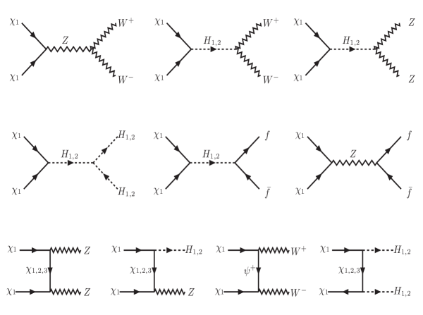
Figure 1: The dominant annihilation channels of DM to SM fields and heavy Higgs in the final states.

The thermally averaged dark matter annihilation cross-section $\langle\sigma|v|\rangle$ is expressed as

$$\begin{split}\langle\sigma|v|\rangle=&\frac{g_{1}^{{}^{\prime}2}}{g_{eff}^{2}}\sigma(\chi_{1}\chi_{1})+2\frac{g^{\prime}_{1}g^{\prime}_{2}}{g_{eff}^{2}}\sigma(\chi_{1}{\chi}_{2})(1+\Delta_{21})^{3/2}exp(-x\Delta_{21})+2\frac{g^{\prime}_{1}g^{\prime}_{3}}{g_{eff}^{2}}\sigma(\chi_{1}{\chi}_{3})(1+\Delta_{31})^{3/2}exp(-x\Delta_{31})\\ &+2\frac{g^{\prime}_{2}g^{\prime}_{3}}{g_{eff}^{2}}\sigma(\chi_{2}{\chi}_{3})(1+\Delta_{21})^{3/2}(1+\Delta_{31})^{3/2}exp(-x(\Delta_{21}+\Delta_{31}))\\ &+2\frac{g^{\prime}_{1}g^{\prime}_{+}}{g_{eff}^{2}}\sigma(\chi_{1}\psi^{+})(1+\Delta_{+1})^{3/2}exp(-x\Delta_{+1})+\frac{g_{+}^{{}^{\prime}2}}{g_{eff}^{2}}\sigma(\psi^{+}\psi^{-})(1+\Delta_{+1})^{3}exp(-2x\Delta_{+1})\\ &+2\frac{g^{\prime}_{2}g^{\prime}_{+}}{g_{eff}^{2}}\sigma(\chi_{2}\psi^{+})(1+\Delta_{+1})^{3/2}(1+\Delta_{21})^{3/2}exp(-x(\Delta_{+1}+\Delta_{21}))\\ &+2\frac{g^{\prime}_{3}g^{\prime}_{+}}{g_{eff}^{2}}\sigma(\chi_{3}\psi^{+})(1+\Delta_{+1})^{3/2}(1+\Delta_{31})^{3/2}exp(-x(\Delta_{+1}+\Delta_{31})\\ &+\frac{g_{2}^{{}^{\prime}2}}{g_{eff}^{2}}\sigma(\chi_{2}{\chi}_{2})(1+\Delta_{21})^{3}exp(-2x\Delta_{21})+\frac{g_{3}^{{}^{\prime}2}}{g_{eff}^{2}}\sigma(\chi_{3}{\chi}_{3})(1+\Delta_{31})^{3}exp(-2x\Delta_{31})\,\,,\end{split}$$ (40)

where $\Delta_{i1}=\frac{{m_{\chi_{i}}}-m_{\chi_{1}}}{m_{\chi_{1}}}$ and $\Delta_{+1}=\frac{m_{\psi}-m_{\chi_{1}}}{m_{\chi_{1}}}$ are the corresponding mass splitting ratios. Therefore it can be easily concluded that for smaller values of mass splitting co-annihilation effects will enhance the final dark matter annihilation cross-section significantly. The effective degrees of freedom $g_{eff}$

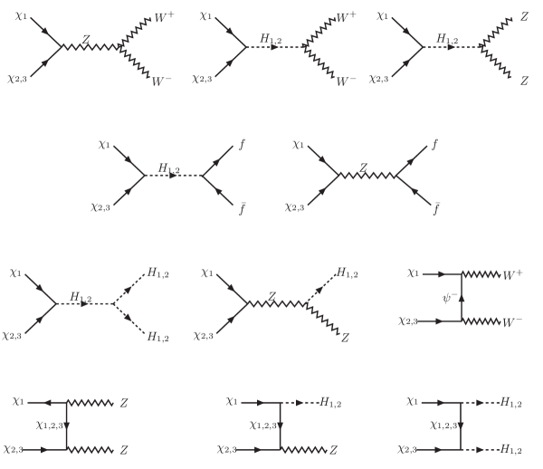
Figure 2: The dominant co-annihilation channels of DM (${\chi}_{1}$) with neutral fermions ${\chi}_{2,3}$.

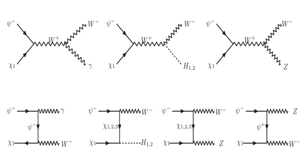
Figure 3: The dominant co-annihilation channels of DM (${\chi}_{1}$) with charged fermion $\psi^{-}$.

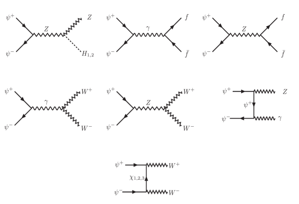
Figure 4: The dominant co-annihilation channels of the charged fermion pair $\psi^{+}$ and $\psi^{-}$.

is denoted as

$$g_{eff}=g^{\prime}_{1}+g^{\prime}_{2}(1+\Delta_{21})^{3/2}exp(-x\Delta_{21})+g^{\prime}_{3}(1+\Delta_{31})^{3/2}exp(-x\Delta_{31})+g^{\prime}_{+}(1+\Delta_{+1})^{3/2}exp(-x\Delta_{+1})\,.$$ (41)

In the above expression $g^{\prime}_{i},i=1-3$ are spin degrees of freedom of particles. Using Eqs.(38-41), relic density of the dark matter ${\chi}_{1}$ can be obtained for the model parameters. The relic density of the dark matter candidate must satisfy the bounds from Planck [97] with $1\sigma$ uncertainty is given as

$$0.1175\leq\Omega_{DM}h^{2}\leq 0.1219\,\,.$$ (42)

4.2 Direct searches for dark matter

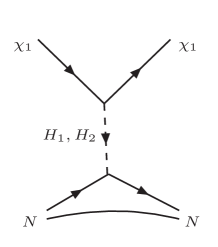
Figure 5: Schematic diagrams for dark matter direct detection processes: left panel: spin independent and right panel: spin dependent processes ($N$ is the nucleon).

Direct detection of dark matter is based on the scattering of the incoming dark matter particle with detector nucleus. In the present scenario, the dark matter candidate $\chi_{1}$ can have both spin independent (SI) and spin dependent (SD) scatterings with the detector. In view of Eq.(27), spin independent interactions are mediated by scalars $H_{1}$ and $H_{2}$ while spin dependent scattering is mediated via neutral gauge boson $Z$ as shown in Fig. 5.

The expression for spin independent direct detection cross-section in the present singlet doublet model is given as [98]

$$\sigma_{SI}\simeq\frac{m_{r}^{2}}{8\pi}\left(\frac{\lambda_{H_{1}\chi_{1}\chi_{1}}\cos{\theta}}{m_{H_{1}}^{2}}-\frac{\lambda_{H_{2}\chi_{1}{\chi}_{1}}\sin{\theta}}{m_{H_{2}}^{2}}\right)^{2}\lambda_{p}^{2}$$ (43)

where $\lambda_{H_{i}\chi_{1}\chi_{1}},\leavevmode\nobreak\ i=1,2$ denotes the coupling of dark matter ${\chi}_{1}$ with the scalar $H_{1}$ and $H_{2}$ as given in the Eq.(27). In the above expression of direct detection cross-section, $m_{r}$ is the reduced mass for the dark matter-nucleon scattering, $m_{r}=\frac{m_{\chi_{1}}m_{p}}{m_{\chi_{1}}+m_{p}}$, $m_{p}$ being the proton mass. The scattering factor $\lambda_{p}$ is expressed as [99]

$$\lambda_{p}=\frac{m_{p}}{v}\left[\sum_{q}f_{q}+\frac{2}{9}\left(1-\sum_{q}f_{q}\right)\right]\simeq 1.3\times 10^{-3}\,\,,$$ (44)

where $f_{q}$ is the atomic form factor[100, 101].

As we have mentioned earlier, following the interaction Lagrangian described in Eq.(27), we have an axial vector interaction of the neutral Majorana fermions with the SM gauge boson $Z$. This will infer spin dependent dark matter nucleon scattering with the detector nuclei. The expression for the spin dependent cross-section is given as [102]

$$\sigma_{SD}=\frac{16m_{r}^{2}}{\pi}\left[\sum_{q=u,d,s}{d_{q}\lambda_{q}}\right]^{2}J_{N}(J_{N}+1).$$ (45)

where $d_{q}\sim\frac{g^{2}}{2c_{W}m_{Z}^{2}}ReX_{11}$ (following Eq.(27)) and $\lambda_{q}$ depends on the nucleus considering ${\chi}_{1}$ as the dark matter candidate.

4.3 Results

In this section we present the dark matter phenomenology involving different model parameters and constrain the parameter space with theoretical and experimentally observed bounds discussed in Sec. 4. As mentioned earlier, the dark matter candidate is a thermal WIMP (Weakly Interacting Massive Particle) in nature. The dark matter phenomenology is controlled by the following parameters ,

$$\{c,\leavevmode\nobreak\ v_{\phi},\leavevmode\nobreak\ \lambda,\leavevmode\nobreak\ \sin\theta,\leavevmode\nobreak\ m_{\psi}\,,\leavevmode\nobreak\ m_{H_{2}}\}.$$

We have used LanHEP (version 3.2) [103] to extract the model files and use MicrOmegas (version 3.5.5) [104] to perform the numerical analysis. The model in general consists of three neutral fermions ${\chi}_{i},\leavevmode\nobreak\ i=1-3$ and one charged fermion $\psi^{+}$ which take part in this analysis. The lightest fermion ${\chi}_{1}$ is the dark matter candidate that annihilates into SM particles and freeze out to provide the required dark matter relic density. The heavier neutral particles in the dark sector ${\chi}_{2,3}$ and the charged particle $\psi$ annihilates into the lightest particle ${\chi}_{1}$. Also ${\chi}_{2,3}$ co-annihilation contributes to the dark matter relic abundance (when the mass differences are small). Different possible annihilation and co-annihilation channels of the dark matter particle is shown in Figs. 1, 2, 3, 4 .

We have kept the mass of the heavier Higgs $m_{H_{2}}$ below 1 TeV from the viewpoint of future experimental search at LHC. In particular, unless otherwise stated, for discussion purpose we have kept the heavy Higgs at 300 GeV. Also note that in this regime, $\sin\theta$ is bounded by $\sin\theta\lesssim 0.3$[74], so we could exploit maximum amount of variation for $\sin\theta$ as otherwise with heavier $H_{2}$ $\sin\theta$ will be more restrictive. In the small $\sin\theta$ approximation, $\lambda_{\phi}$ almost coincides with the second term in Eq.(25). Now it is quite natural to keep the magnitude of a coupling below unity to maintain the perturbativity at all energy scales (including its running). Hence with the demand $\lambda_{\phi}<1$, from Eq.(25) one finds $v_{\phi}>\sqrt{3}m_{H_{2}}$.

4.3.1 Study of importance of individual parameters

Now we would like to investigate how the relic density and direct detection cross-section depend on different parameters of the set-up. For this purpose, in Fig. 6 (left panel) we plot the variation of DM mass $m_{\chi_{1}}$ with relic density for four different values of Yukawa coupling $\lambda$ while $m_{\psi}$ is taken to be 500 GeV. The vev of the singlet scalar $\phi$ is varied from 500 GeV to 10 TeV. Fig. 6 (right panel) corresponds to a different $m_{\psi}=1000$ GeV. Other parameters $m_{{\rm{H}}_{2}},\sin\theta$ and $c$ are kept fixed at 300 GeV, 0.1 and 0.1 respectively as indicated on top of each figures. Note that $c=0.1$ is a natural choice from the viewpoint that it remains non-perturbative even at very high scale. The horizontal black lines in both the figures denote the required dark matter relic abundance. In producing Fig. 6, dark matter direct detection limits from both spin independent and spin dependent searches are included. The solid (colored) portion of a curve correspond to the range of $m_{\chi_{1}}$ which satisfies the SI direct detection (DD) bounds while the dotted portion exhibits the disallowed range using DD limits.

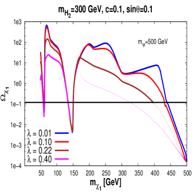
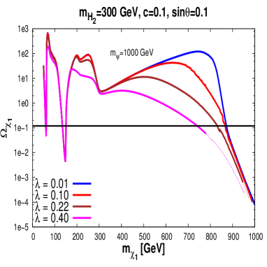
Figure 6: DM relic density as a function of DM mass for [left panel:] $m_{\psi}=$ 500 GeV and [right panel:] $m_{\psi}=$ 1000 GeV with different choices of $\lambda=$ 0.01 (blue), 0.1 (red), 0.25 (brown) and 0.4 (pink). Values of heavy Higgs mass, scalar mixing angle and $c$ have been kept fixed at $m_{H_{2}}=300$ GeV, $\sin\theta=0.1$ and $c=0.1$. Dotted portions indicate the disallowed part from SI direct detection cross-section limit.

From Fig. 6, we also observe that apart from the two resonances, one for the SM Higgs and other for the heavy Higgs, the dark matter candidate satisfies the required relic density in another region with large value of $m_{\chi_{1}}$. For example, with $\lambda=0.22$, the relic density and DD cross-section is marginally satisfied by $m_{\chi_{1}}\sim$ 400 GeV. The presence of this allowed value of dark matter mass is due to the fact that the co-annihilation processes turn on (they become effective when $\Delta_{i1}/m_{\chi_{1}}\sim 0.1$ or less) which increases the effective annihilation cross-section $\langle\sigma|v|\rangle$ and hence a sharp fall in relic density results. Since both annihilation and co-annihilations are proportional to $\lambda$ (see Eq.(27)), an increase in $\lambda$ (from pink to red lines) leads to decrease in relic density (for a fixed dark matter mass) and this would correspond to smaller value of $m_{\chi_{1}}$ for the satisfaction of the relic density apart from resonance regions. For example, with $\lambda=0.1$ or 0.01, relic density and DD satisfied value of $m_{\chi_{1}}$ is shifted to $\sim$ 440 GeV compared to $m_{\chi_{1}}\sim 400$ GeV with $\lambda=0.22$. It can also be traced that there exist couple of small drops of relic density near $m_{\chi_{1}}\sim 212$ GeV and 300 GeV. This is mostly prominent for the line with small $\lambda$ (=0.1 (red line) and 0.01 (blue line)). While the first drop indicates the opening of the final states $H_{1}H_{2}$, the next one is due to the appearance of $H_{2}H_{2}$ final states.

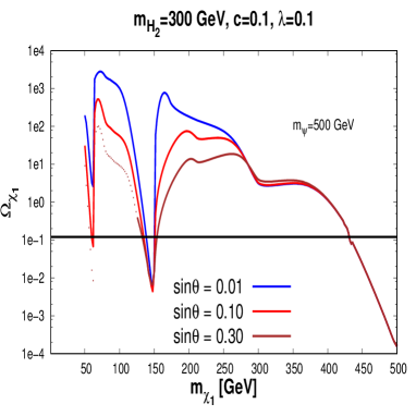
Figure 7: DM relic density as a function of DM mass considering [left panel:] $m_{\psi}=$ 500 GeV and [right panel:] $m_{\psi}=$ 1000 GeV for different choices of scalar mixing angle $\sin\theta\sim$ 0.01 (blue), 0.1 (red) and 0.3 (brown). Values of other parameters have been fixed at $m_{H_{2}}=300$ GeV, $\lambda=0.1$ and $c=0.1$. Dotted portions indicate the disallowed part from SI direct detection cross-section limit.

In the present dark matter model, we found that the regions that satisfy dark matter relic density has spin dependent cross-section $\sim 10^{-42}-10^{-44}$ cm² which is well below the present limit obtained from spin dependent bounds (for the specific mass range of dark matter we are interested in) from direct search experiments [67]. Therefore, it turns out that the spin independent scattering of dark matter candidate is mostly applicable in restricting the parameter space of the present model.

In Fig. 7, we depict the effect of scalar mixing in dark matter phenomenology keeping parameters $c$ and $\lambda$ both fixed at 0.1 along with the same values of $m_{\psi}$ and $m_{H_{2}}$ used in Fig. 6. The vev $v_{\phi}$ is varied within the range $500\leavevmode\nobreak\ {\rm GeV}\leq v_{\phi}\leq 10\leavevmode\nobreak\ {\rm TeV}$. Similar to Fig. 6 (there with $\lambda$), here also we notice a scaling with respect to different values of $\sin\theta$ as the dark matter annihilations depend upon it and there exist two resonances. However beyond $m_{\chi_{1}}\sim 250$ GeV, dependence on $\sin\theta$ mostly disappears as seen from the Fig. 7 as we observe all three lines merge into a single one. Note that this is also the region where co-annihilations start to become effective as explained in the context of Fig. 6. It turns out that due to the presence of axial type of coupling in the Lagrangian (see Eq.(27)), the co-annihilation processes with final state particles including $W^{\pm}$ and $Z$ bosons are most significant and they are independent of the scalar mixing $\theta$. It therefore explains the behavior of the red (with $\sin\theta=0.01$), green (with $\sin\theta=0.1$) and blue (with $\sin\theta=0.2$) lines in Fig. 7.

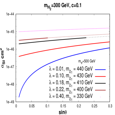
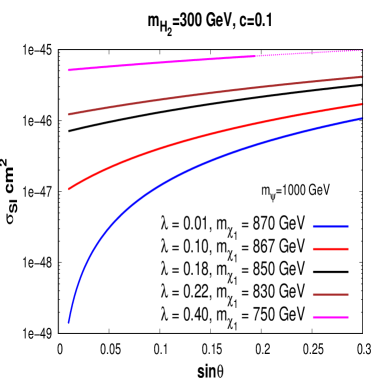
Figure 8: Effects of scalar mixing angle for different values of $\lambda\sim$ 0.01 (blue), 0.1 (red), 0.18 (black), 0.22 (brown), 0.4 (pink) on dark matter spin independent direct detection cross-section for [left panel:] $m_{\psi}=500$ GeV and [right panel:] $m_{\psi}=1000$ GeV. Values of other parameters have been fixed at $m_{H_{2}}=300$ GeV and $c=0.1$. Dotted portions indicate the disallowed part from SI direct detection cross-section limit.

From Fig. 7, it is observed that scalar mixing has not much role to play in the co-annihilation region. However the scalar mixing has significant effect in the direct detection (DD) of dark matter. To investigate the impact of $\sin\theta$ on DD cross-section of DM, we choose few benchmark points (set of $\lambda,m_{\chi_{1}}$ values) in our model that satisfy DM relic density excluding the resonance regions ($m_{\chi_{1}}\simeq m_{H_{1}}/2$ resonance regime is highly constrained from invisible Higgs decay limits from LHC). Here we vary scalar mixing from 0.01 to 0.3.

In Fig. 8, we show the variation of spin independent dark matter direct detection cross-section ($\sigma_{SI}$) against $\sin\theta$ for those chosen benchmark values of dark matter mass. Keeping parameters $c$ and $m_{H_{2}}$ fixed at values 0.1 and 300 GeV respectively, $m_{\psi}$ is considered at 500 GeV for the left panel and at 1000 GeV for the right panel of Fig. 8. Among these five benchmark sets, four of them (except $\lambda=0.18$, $m_{\chi_{1}}=410$ GeV) were already present in the of Fig. 6 (corresponding to $\sin\theta=0.1$). Five lines (blue, red, black, brown and pink colored ones corresponding to different sets of values of $\lambda$ and $m_{\chi_{1}}$) describe the DD cross-section dependence with $\sin\theta$. It is interesting to observe that with higher $\lambda$, there exists an increasing dotted portion on the curves (e.g. in brown colored line for $m_{\psi}=500$ GeV, it starts from $\sin\theta>0.1$, which stands for the non-satisfaction of the parameter space by the DD limits. This behaviour can be understood in the following way. From Eq.(43), it is clear that the first term dominates and hence an increase of SI DD cross-section with respect to larger $\sin\theta$ value (keeping other parameters fixed) is expected as also evident in the

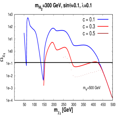
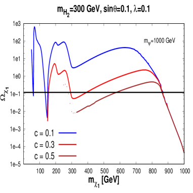
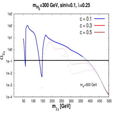
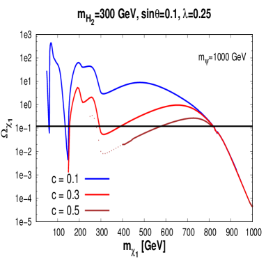
Figure 9: Dark matter relic density as a function of DM mass with different choices of $c\sim$ 0.1 (blue), 0.3 (red), 0.5 (brown) for [top left:] $m_{\psi}=500$ GeV, $\lambda=0.1$, [top right:] $m_{\psi}=1000$ GeV, $\lambda=0.1$, [bottom left:] $m_{\psi}=500$ GeV, $\lambda=0.0.25$ and [bottom right:] $m_{\psi}=1000$ GeV, $\lambda=0.25$. Values of other parameters have been kept fixed at $m_{H_{2}}=300$ GeV and $\sin\theta=0.3$. Dotted portions indicate the disallowed part from SI direct detection cross-section limit.

figures. We do not include the spin dependent cross-section here; however checked that it remains well within the observed limits.

In Fig. 9, we plot the dark matter relic density against dark matter mass for different values of $c$ keeping other parameters fixed and using the same range of $v_{\phi}$ (500 GeV - 10 TeV) as considered in earlier plots. The top (bottom) left panel of Fig. 9 corresponds to $m_{\psi}=500$ GeV and top (bottom) right panel are plotted for $m_{\psi}=1000$ GeV. Curves with higher value of $c$ start with larger initial value of dark matter mass. This can be understood easily from mass matrix $\mathcal{M}$ of Eq.(7), as large

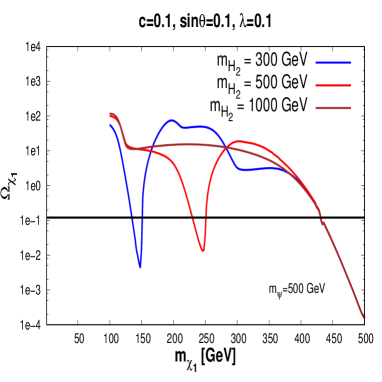
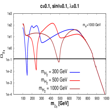
Figure 10: Relic density of dark matter as a function of DM mass for different values of $m_{H_{2}}=300$ GeV (blue), 500 GeV (red) and 1000 GeV (brown) with [left panel:] $m_{\psi}=$ 500 GeV and [right panel:] $m_{\psi}=$ 1000 GeV. The other parameters $c$, $\lambda$ and $\sin\theta$ are kept fixed at 0.1.

$m_{\psi}$ with small $v_{\phi}$ and $\lambda$, dark matter mass $\sim cv_{\phi}$. Hence as $c$ increases, the DM mass starts from a higher value. The upper panel of figures is for $\lambda=0.1$ and the lower panel stands for $\lambda=0.25$.

We observe from Fig. 9 that enhancing $c$ reduces DM relic density particularly for the region where DM annihilation processes are important. At some stage co-annihilation, in particular, processes with final states including SM gauge fields takes over which is mostly insensitive to $c$. Hence all different curves join together. This is in line with observation in Fig. 7 as well. Here also

we notice that all the curves have fall around 212 GeV and 300 GeV where DM DM $\rightarrow H_{1},H_{2}$ and DM DM $\rightarrow H_{2},H_{2}$ channels open up respectively. We observe that with a higher value of $c$, for example with $c=0.5$ in Fig. 9 (top left panel), the $DMDM\rightarrow H_{2}H_{2}$ annihilation becomes too large and also disallowed by the DD bounds as indicated by dotted lines. We therefore infer that the satisfaction of the DD bounds and the DM relic density prefer a lower value of $c$ which is also consistent with the perturbativity point of view. Increasing the Yukawa coupling $\lambda$ will change the above scenario, as depicted in lower panel of Fig. 9. We found that such effect is prominent for smaller values of $m_{\psi}$ while compared top and bottom left panels of Fig. 9.

So far, in Figs. 6-9, we have presented the variations of DM relic density with DM mass keeping the mass of heavy scalar $H_{2}$ fixed. In Fig. 10 (left panel), we show the variation of DM relic density against $m_{\chi_{1}}$ for three different values of $m_{H_{2}}=300,500,1000$ GeV with fixed values of $c,\leavevmode\nobreak\ \lambda,\leavevmode\nobreak\ \sin\theta$ (all set to the value 0.1) with $m_{\psi}=500$ GeV. The vev $v_{\phi}$ is varied from 1 TeV to 10 TeV. From Fig. 10 (left panel), we note that each plot for a specific $m_{H_{2}}$ follow the same pattern as in previous figures. Here we notice that with different $m_{H_{2}}$, the heavy Higgs resonance place ($m_{\chi_{1}}\sim m_{H_{2}}/2)$

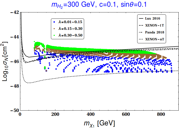
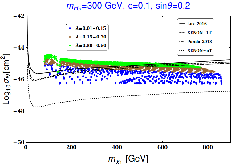
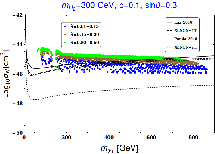
Figure 11: SI direct detection cross-section is plotted against DM mass for relic density satisfied points for [top left:] $\sin\theta=0.1$, [top right:] $\sin\theta=0.2$ and [bottom:] $\sin\theta=0.3$. The other parameters $c=0.1$ and $m_{H_{2}}=300$ GeV have been kept fixed. Bounds from LUX 2016, XENON 1T, PANDA 2018, XENON-nT are also included in the plot.

is only affected. For large $m_{H_{2}}$ (say for 1000 GeV), the resonance point disappears as it falls within the co-annihilation dominated region. A similar plot using the same set of parameters and value of $m_{H_{2}}$ but with $m_{\psi}=1000$ GeV in Fig. 10 (right panel) clearly shows this. In this case, we have a prominent resonance region for $m_{H_{2}}=1000$ GeV as the co-annihilation takes place at a higher value of dark matter mass with the increase in $m_{\psi}$. It is to be mentioned once again that in all the above plots (Figs. 6-10), solid regions indicate the satisfied region and dotted region indicates the disallowed region for DM mass by spin independent direct detection cross-section bounds.

4.3.2 Constraining $\lambda-\sin\theta$ from a combined scan of parameters

A more general result for the present dark matter model can be obtained by varying the mass of charged fermion $m_{\psi}$, vev $v_{\phi}$ of the heavy singlet scalar field and the Yukawa coupling $\lambda$. We use the LEP bound on chargino mass to set the lower limit on the mass of charged fermion $m_{\psi}\gtrsim 100$ GeV [90]. Using this limit on charged fermion mass, we scan the parameter space of the model with the following set of parameters

$$100\leavevmode\nobreak\ {\rm GeV}\lesssim m_{\psi}\lesssim 1000\leavevmode\nobreak\ {\rm GeV};\leavevmode\nobreak\ 500\leavevmode\nobreak\ {\rm GeV}\lesssim v_{\phi}\lesssim 10\leavevmode\nobreak\ {\rm TeV};\leavevmode\nobreak\ 0.01\lesssim\lambda\lesssim 0.5;$$

$$\textrm{ }\sin\theta\leavevmode\nobreak\ =\leavevmode\nobreak\ 0.1,0.2,0.3;\leavevmode\nobreak\ c=0.1;\leavevmode\nobreak\ \leavevmode\nobreak\ m_{H_{2}}=300\leavevmode\nobreak\ {\rm GeV.}$$ (46)

In Fig. 11 (top left panel) we plot the values of DM mass against dark matter spin independent cross-section for the above mentioned ranges of parameters with $\sin\theta=0.1$ which already satisfy DM relic abundance obtained from Planck [97]. Different ranges of the Yukawa coupling $\lambda$ are shown in blue (0.01-0.15), brown (0.15-0.30) and green (0.30-0.50) shaded regions.

The bounds on DM mass and SI direct detection scattering cross-section from LUX[17], XENON-1T[18], Panda 2018[19] and XENON-nT[20] are also shown for comparison. The spin dependent scattering cross-section for the allowed parameter space is found to be in agreement with the present limits from Panda 2018[19] and does not provide any new constraint on the present phenomenology. From Fig. 11 (top left panel) it can also be observed that increasing $\lambda$ reduces the region allowed by the most stringent Panda 2018 limit. This is due to the fact that an increase in $\lambda$ enhances the dark matter direct detection cross-section as we have clearly seen from previous plots (see Fig. 6). Here we observe that with the specified set of parameters, dark matter with mass above 100 GeV is consistent with DD limits with $\lambda=0.01-0.15$ (see the blue shaded region). For the brown region, we conclude that with $\lambda=0.15-0.30$, DM mass above 400 GeV is allowed and with high $\lambda=0.30-0.50$, DM with mass 600 GeV or more is only allowed. We also note that a large region of the allowed parameter space is ruled out when XENON-nT [20] direct detection limit is taken into account.

Similar plots for the same range of parameters given in Eq.(46) for $\sin\theta=0.2$ and 0.3 are shown in top right panel and bottom panel of Fig. 11 respectively. These plots depict the same nature as observed in top left panel of Fig. 11. In all these plots, the low mass region ($m_{\chi_{1}}\lesssim 62.5$ GeV) is excluded due to invisible decay bounds on Higgs and $Z$. It can be observed comparing all three plots in Fig. 11, that the allowed region of DM satisfying relic density and DD limits by Panda 2018 becomes shortened with the increase $\sin\theta$. In other words, it prefers a larger value of DM mass with the increase of $\sin\theta$. This is also expected as the increase of $\sin\theta$ is associated with larger DD cross-section (due to $H_{1},H_{2}$ mediated diagram). Hence overall we conclude from this DM phenomenology that increase of both $\lambda$ and $\sin\theta$ push the allowed value of DM mass toward a high value. In terms of vacuum stability, these two parameters, the Yukawa coupling $\lambda$ and the scalar mixing $\sin\theta$, affect the Higgs vacuum stability differently. The Yukawa coupling destabilizes the Higgs vacuum while the scalar mixing $\sin\theta$ makes the vacuum more stable. Detailed discussion on the Higgs vacuum stability is presented in the next section.

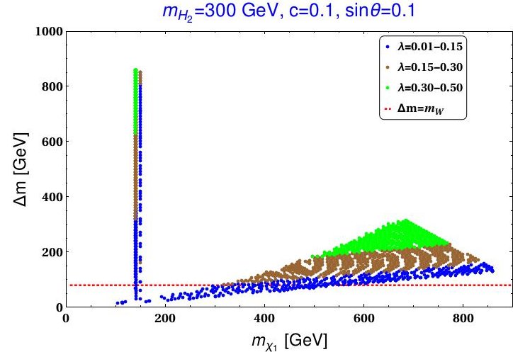
Figure 12: Mass difference between DM and the charged fermion $\Delta m$ is plotted against $m_{\chi_{1}}$ for different sets of $\lambda\sim$ 0.01-0.15 (blue), 0.15-0.30 (brown) and 0.30-0.50 (green) with $\sin\theta=0.1$. All points satisfy the relic density direct detection cross-section bound from PANDA 2018. The other parameters are kept fixed at $c=0.1$ and $m_{H_{2}}=300$ GeV. The red line indicates the $W$ boson mass ($m_{W}$).

A general feature of the singlet doublet model is the existence of two other neutral fermions, $\chi_{2,3}$ and a charged fermion, $\psi^{+}$. All these participate in the co-annihilation process which contributes to the relic density of the dark matter candidate, $\chi_{1}$. The charged fermion $\psi^{+}$ can decay into $W^{+}$ and $\chi_{1}$, when the mass splitting $\Delta m=m_{\psi}-m_{\chi_{1}}$ is larger than $W^{+}$ mass. However, for mass splitting $\Delta m$ between $\chi_{1}$ and $\psi^{+}$ smaller than the mass of gauge boson $W^{+}$, the three body decay of charged fermion, $\psi^{+}$ into ${\chi}_{1}$ associated with lepton and neutrino becomes plausible. This three body decay must occur before ${\chi}_{1}$ freezes out, otherwise it would contribute to the relic. Therefore, the decay lifetime of $\psi^{+}$ should be smaller compared to the freeze out time of ${\chi}_{1}$. The freeze out of the dark matter candidate ${\chi}_{1}$ takes place at temperature $T_{f}=m_{\chi_{1}}/20$. Therefore, the corresponding freeze out time can be expressed as

$$t=1.508g_{\star}^{-\frac{1}{2}}M_{P}/T_{f}^{2}\,\,,$$ (47)

where $M_{P}$ is the reduced Planck mass $M_{P}=2.435\times 10^{18}$ GeV and $g_{\star}$ is effective number of degrees of freedom. The decay lifetime of the charged fermion $\psi^{+}$ is given as $\tau_{\psi^{+}}=\frac{1}{\Gamma_{\psi^{+}}}$, where $\Gamma_{\psi^{+}}$ is the decay width for the decay $\psi^{+}\rightarrow{\chi}_{1}l^{+}\bar{\nu}_{l}$, is of the form

$$\Gamma_{\psi^{+}} = \frac{G_{F}^{2}}{12\pi^{3}}\left[(V_{31}^{2}+V_{21}^{2})\{-2m_{\psi}m_{\chi_{1}}^{2}I_{1}+3(m_{\psi}^{2}+m_{\chi_{1}}^{2})I_{2}-4m_{\psi}I_{3}\}\right.$$ (48)

$$\left.+12V_{31}V_{21}\{m_{\chi_{1}}(m_{\psi}^{2}+m_{\chi_{1}}^{2})I_{1}-2m_{\psi}m_{\chi_{1}}I_{2}\}\right]\,\,.$$

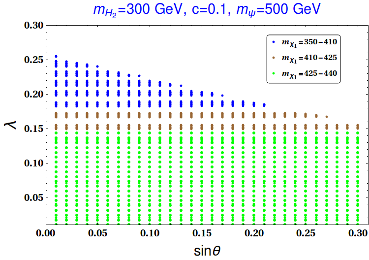
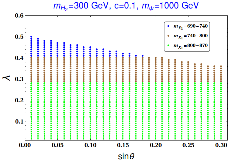
Figure 13: Correlation between $\lambda$ and $\sin\theta$ for both relic and direct detection cross-section satisfied points with [left panel:] $m_{\psi}=500$ GeV and [right panel:] $m_{\psi}=1000$ GeV. The other parameters are kept fixed at $c=0.1$, $m_{H_{2}}=300$ GeV. Different ranges of $m_{\chi_{1}}$ (in GeV) are shown with color codes as mentioned in the inset.

In the above expression, $G_{F}$ is the Fermi constant and the terms $I_{1,2,3}$ is expressed as

$$I_{1}=\int\sqrt{x^{2}-a^{2}}dx,\leavevmode\nobreak\ \leavevmode\nobreak\ I_{2}=\int x\sqrt{x^{2}-a^{2}}dx,\leavevmode\nobreak\ \leavevmode\nobreak\ I_{3}=\int x^{2}\sqrt{x^{2}-a^{2}}dx\,\,$$ (49)

where $x=E_{\chi_{1}}$ and $a=m_{\chi_{1}}$, $E_{\chi_{1}}$ being the total energy of $\chi_{1}$.

In order to satisfy the condition that $\psi^{+}$ decays before the freeze out of ${\chi}_{1}$, one must have $\tau_{\psi_{+}}\leq t$. The integrals $I_{1,2,3}$ in Eq.(49) are functions of mass splitting $\Delta m$ and so is the total decay width $\Gamma_{\psi^{+}}$. To show the dependence on $\Delta m$, we present a correlation plot $m_{\chi_{1}}$ against $\Delta m$ in Fig. 12. Fig. 12 is plotted for the case $\sin\theta=0.1$ (consistent with Fig. 11 having the region allowed by the DD bound from Panda 2018). We use the same color code for $\lambda$ as shown in Fig. 11. The horizontal red line indicates the the region where $\Delta m=m_{W}$. From Fig. 12 we observe that for smaller values of $\lambda$ (0.01-0.15), $\Delta m<m_{W}$ is satisfied upto $m_{\chi_{1}}\sim 500$ GeV. The mass splitting increases for larger $\lambda$ values. We find that for the chosen range of model parameters (Eq.(46)), the decay life time $\tau_{\psi^{+}}$ is several order of magnitudes smaller than the freeze out time of $\chi_{1}$.

We end this section by estimating the value of $T$ parameter in Table 2 for two sets of relic satisfied points (with $\lambda=0.4$ and 0.18) as we mentioned before that among the $S,T$ and $U$, only $T$ would be relevant in this scenario.

$c$	$m_{\psi}(GeV)$	$v_{\phi}$ (TeV)	$m_{\chi_{1}}$ (GeV)	$\lambda$	T$\times 10^{-4}$
0.1	1000	7.55	750	$0.4$	$1$
0.1	500	4.20	410	$0.28$	$0.1$

Table 2: Values of T-parameter induced by extra fermions in the set up for two sets of relic density satisfied points (see Fig. 8).

With further smaller $\lambda$, $T$ parameter comes out to be very small and hence it does not pose any stringent constraint on the relic satisfied parameter space. However with large $\lambda\sim 1$, the situation may alter.

In our scenario, we have also seen in Fig. 6 that for value of $\lambda$ larger than 0.4, the direct detection cross-section of dark matter candidate also increases significantly and are thereby excluded by present limits on dark matter direct detection cross-section. To make this clear, here we present a plot, Fig. 13 (left panel), of relic density and DD satisfied points in the $\sin\theta-\lambda$ plane, where the other parameters are fixed at $c=0.1,m_{\psi}=500$ GeV, $m_{H_{2}}=300$ GeV. As before, $v_{\phi}$ is varied between 500 GeV and 10 TeV. Similar plot with same set of $c,\leavevmode\nobreak\ m_{H_{2}}$ but with $m_{\psi}=1000$ GeV is depicted in right panel of Fig. 13. Different ranges of dark matter masses are specified with different colors as mentioned in the caption of Fig. 13. From Fig. 13 we observe that allowed range of $\lambda$ reduces with the increase of scalar mixing due to the DD bounds. From Fig. 13 (left panel) we get a maximum allowed $\lambda\sim 0.25$ while the same for the $m_{\psi}=1000$ GeV (right panel) turns out to be $\lambda=0.5$. Furthermore as we will see the study of vacuum stability, discussed in Sec. 5, indicates that the Yukawa coupling $\lambda$ should not be large in order to maintain the electroweak vacuum absolutely stable till Planck scale. Therefore, larger values of $\lambda$ (close to 1) is not favoured in the present scenario.

5 EW vacuum stability

In the present work consisting of singlet doublet dark matter model with additional scalar, we have already analysed (in previous section) the parameter space of the set-up using the relic density and direct detection bounds. Here we extend the analysis by examining the Higgs vacuum stability within the framework. It is particularly interesting as the framework contains two important parameters, (i) coupling of dark sector fermions with SM Higgs doublet ($\lambda$) and (ii) mixing (parametrized by angle $\theta$) between the singlet scalar and SM Higgs doublet. The presence of these two will modify the stability of the EW vacuum. First one makes the situation worse than in the SM by driving the Higgs quartic coupling $\lambda_{H}$ negative earlier than $\Lambda_{I}^{\textrm{SM}}$. The second one, if sufficiently large, can negate the effect of first and make the Higgs vacuum stable. Thus the stability of Higgs vacuum depends on the interplay between these two. Moreover, as we have seen, the scalar singlet also enriches the dark sector with several new interactions that significantly contribute to DM phenomenology satisfying the observed relic abundance and direct detection constraint. Also the scalar mixing angle is bounded by experimental constraints ($\sin\theta\lesssim 0.3$) as we have discussed in Sec. 3.

The proposed set up has two additional mass scales: the DM mass ($m_{\chi_{1}}$) and heavy Higgs ($m_{H_{2}}$). Although the dark sector has four physical fermions (three neutral and one charged), we can safely ignore the mass differences between them when we consider our DM to fall outside the two resonance regions (Figs. 6-10). As we have seen in this region (see Fig. 12), co-annihilation becomes dominant, all the masses in the dark sector fermions are close enough ($\sim m_{\chi_{1}}$, see Figs. 6-10). Hence the renormalisation group (RG) equations will be modified accordingly from SM ones with the relevant couplings entering at different mass scales. Here we combine the RG equations (for the relevant couplings only) [105] together in the following (provided $\mu>m_{\phi},m_{\chi_{1}}$),

$$\frac{dg_{1}}{dt} =\beta^{\textrm{SM}}_{g_{1}}+\frac{1}{16\pi^{2}}\frac{2}{3}g_{1}^{3},$$ (50)

$$\frac{dg_{2}}{dt} =\beta^{\textrm{SM}}_{g_{2}}+\frac{1}{16\pi^{2}}\frac{2}{3}g_{2}^{3},$$ (51)

$$\frac{d\lambda_{H}}{dt} =\beta^{\textrm{SM}}_{\lambda_{H}}+\frac{1}{16\pi^{2}}\Big{\{}\frac{\lambda_{\phi H}^{2}}{2}\Big{\}}+\frac{1}{16\pi^{2}}\Big{\{}-2\lambda^{4}+4\lambda_{H}\lambda\Big{\}},$$ (52)

$$\frac{dy_{t}}{dt} =\beta^{\textrm{SM}}_{y_{t}}+\frac{1}{16\pi^{2}}\Big{\{}\lambda^{2}y_{t}\Big{\}},$$ (53)

$$\frac{d\lambda}{dt} =\frac{1}{16\pi^{2}}\Big{\{}\lambda(3y_{t}^{2}-\frac{3}{4}g_{1}^{2}-\frac{9}{4}g_{2}^{2})+\frac{5}{2}\lambda^{3}\Big{\}},$$ (54)

$$\frac{d\lambda_{\phi H}}{dt} =\frac{1}{16\pi^{2}}\Big{\{}12\lambda_{H}\lambda_{\phi H}+6\lambda_{\phi}\lambda_{\phi H}+4\lambda_{\phi H}^{2}+6y_{t}^{2}\lambda_{\phi H}-\frac{3}{2}g_{1}^{2}\lambda_{\phi H}-\frac{9}{2}g_{2}^{2}\lambda_{\phi H}+2\lambda^{2}\lambda_{\phi H}+2c^{2}\lambda_{\phi H}\Big{\}},$$

$$\frac{d\lambda_{\phi}}{dt} =\frac{1}{16\pi^{2}}\Big{\{}18\lambda_{\phi}^{2}+2\lambda_{\phi H}^{2}-\frac{1}{2}c^{4}+4\lambda_{\phi}c^{2}\Big{\}},$$ (55)

$$\frac{dc}{dt} =\frac{1}{16\pi^{2}}\Big{\{}6c^{3}\Big{\}},$$ (56)

where $\beta^{\textrm{SM}}$ is the SM $\beta$ function (in three loop) of respective couplings [3, 106, 107, 108].

In this section our aim is to see whether we can achieve SM Higgs vacuum stability till Planck mass ($M_{P}$). However we have two scalars (SM Higgs doublet and one gauge singlet $\phi$) in the model. Therefore we should ensure the boundedness or stability of the entire scalar potential in any field direction. In that case the following matrix

$$\begin{pmatrix}\lambda_{H}&\frac{\lambda_{\phi H}}{2}\\ \frac{\lambda_{\phi H}}{2}&\lambda_{\phi}\\ \end{pmatrix},$$ (57)

has to be co-positive. The conditions of co-positivity [75, 76] of such a matrix is provided by

$$\lambda_{H}(\mu)>0,\textrm{ }\lambda_{\phi}(\mu)>0,\textrm{ and }\lambda_{\phi H}(\mu)+2\sqrt{\lambda_{H}(\mu)\lambda_{\phi}(\mu)}>0.$$ (58)

Violation of $\lambda_{H}>0$ could lead to unbounded potential or existence of another deeper minimum along the Higgs direction. The second condition ($\lambda_{\phi}(\mu)>0$) restricts the scalar potential from having any runway direction along $\phi$. Finally, $\lambda_{\phi H}(\mu)+2\sqrt{\lambda_{H}(\mu)\lambda_{\phi}(\mu)}>0$ ensures the potential to be bounded from below or non-existence of another deeper minimum somewhere between $\phi$ or $H$ direction.

On the other hand, if there exists another deeper minimum other than the EW one, the estimate of the tunneling probability $P_{T}$ of the EW vacuum to the second minimum is essential. The Universe will be in metastable state only, provided the decay time of the EW vacuum is longer than the age of the Universe. The tunneling probability is given by [3, 9],

$$P_{T}=T_{U}^{4}\mu_{B}^{4}e^{-\frac{8\pi^{2}}{3|\lambda_{H}(\mu_{B})|}}.$$ (59)

where $T_{U}$ is the age of the Universe, $\mu_{B}$ is the scale at which probability is maximized, determined from $\beta_{\lambda_{H}}=0$. Hence metastable Universe requires [3, 9]

$$\lambda_{H}(\mu_{B})\leavevmode\nobreak\ >\leavevmode\nobreak\ \frac{-0.065}{1-\textrm{ln}\Big{(}\frac{v}{\mu_{B}}\Big{)}}.$$ (60)

As noted in [3], for $\mu_{B}>M_{P}$, one can safely consider $\lambda_{H}(\mu_{B})=\lambda_{H}(M_{P})$.

The RG improved effective Higgs potential (at high energies $H_{0}\gg v$) can be written as [109, 4]

$$V_{H}^{\textrm{eff}}=\frac{\lambda_{H}^{\textrm{eff}}(\mu)}{4}H_{0}^{4},$$ (61)

with $\lambda_{H}^{\textrm{eff}}(\mu)=\lambda_{H}^{\textrm{SM, eff}}(\mu)+\lambda_{H}^{\phi,\textrm{eff}}(\mu)+\lambda_{H}^{(\psi_{D_{1}},\psi_{S},)\textrm{eff}}(\mu)$ where $\lambda_{H}^{\textrm{SM, eff}}$ is the Standard Model contribution to $\lambda_{H}$. The other two contributions $\lambda_{H}^{\phi,\textrm{eff}}$ and $\lambda^{(\psi_{D_{1}},\chi),\textrm{eff}}$ are due to the newly added fields in the present model as provided below.

$$\lambda_{H}^{\phi,\textrm{eff}}(\mu)=e^{4\Gamma(H_{0}=\mu)}\Big{[}\frac{\lambda_{\phi H}^{2}}{64\pi^{2}}\Big{(}\textrm{ln}\frac{\lambda_{\phi H}}{2}-\frac{3}{2}\Big{)}\Big{]},$$ (62)

$$\lambda_{H}^{(\psi_{D_{1}},\chi),\textrm{eff}}(\mu)=e^{4\Gamma(H_{0}=\mu)}\Big{[}\frac{\lambda^{4}}{16\pi^{2}}\Big{(}\textrm{ln}\frac{\lambda}{2}-\frac{3}{2}\Big{)}\Big{]}.$$ (63)

Here $\Gamma(H_{0})=\int_{m_{t}}^{H_{0}}\gamma(\mu)d\textrm{ln}\mu$, $\gamma(\mu)$ is the anomalous dimension of the Higgs field[3].

In SM, the top quark Yukawa coupling ($y_{t}$) drives the Higgs quartic coupling to negative values. In our set up, the coupling $\lambda$ has very similar effect on $\lambda_{H}$ in Eq.(52). So combination of both $y_{t}$ and $\lambda$ make the situation worse (by driving Higgs vacuum more towards instability) than in SM. However due to the presence of extra singlet scalar, $\lambda_{H}$ gets a positive threshold shift (second term in Eq.(24) at energy scale $m_{H_{2}}$. Also the RG equation of $\lambda_{H}$ is aided by a positive contribution from the interaction of SM Higgs with the extra scalar ($\lambda_{\phi H}$). Here we study whether these two together can negate the combined effect of $y_{t}$ and $\lambda$ leading to $\lambda_{H}^{\textrm{eff}}>0$ for all energy scale running from $m_{t}$ to $M_{P}$. Note that the threshold shift (second term in Eq.(24)) in $\lambda_{H}$ is function of $m_{H_{2}}$ and $\sin\theta$. On the other hand, other new couplings relevant for study of EW vacuum stability are $\lambda_{\phi}$ and $\lambda_{\phi H}$ which can be evaluated from the values of $m_{H_{2}}$, $v_{\phi}$ and $\sin\theta$ through Eq.(25) and Eq.(26). Hence once we fix $m_{H_{2}}$ and use the SM values of Higgs and top mass, the stability analysis effectively depends on $\lambda$, $\sin\theta$ and $v_{\phi}$. We run the three loop RG equations for all the SM couplings and one loop RG equations for the other relevant couplings in the model from $\mu=m_{t}$ to $M_{P}$. We use the boundary conditions of SM couplings as provided in Table 3. The boundary values have been evaluated in [3] by taking various threshold corrections at $m_{t}$ and mismatch between top pole mass and $M\bar{S}$ renormalised couplings into account.

Scale	$y_{t}$	$g_{1}$	$g_{2}$	$g_{3}$	$\lambda_{H}$
$\mu=m_{t}$	$0.93610$	$0.357606$	$0.648216$	$1.16655$	$0.125932$

Table 3: Values of the relevant SM couplings (top-quark Yukawa $y_{t}$, gauge couplings $g_{i}$ and $\lambda_{H}$) at energy scale $\mu=m_{t}=173.2$ GeV with $m_{h}\leavevmode\nobreak\ (m_{H_{1}})=125.09$ GeV and $\alpha_{S}(m_{Z})=0.1184$.

6 Phenomenological implications from DM analysis and EW vacuum stability

We have already found the correlation between $\lambda$ and $\sin\theta$ to satisfy the relic abundance and spin independent DD cross-section limits on DM mass as displayed in Fig. 13. It clearly shows that for comparatively larger value of $\lambda$, upper limit on $\sin\theta$ from DD cross-section is more restrictive. On the other hand, a relatively large value of $\lambda$ affects the EW vacuum stability adversely. In this regard, a judicious choice of reference points from Fig. 13 is made in fixing benchmark points (BP-I of Table 4, corresponding to left panel of Fig. 13 and BP-II of Table 4 corresponding to right panel of Fig. 13). BP-I and BP-II involve moderate values of $\lambda$ for which DD-limits starts constraining $\sin\theta$ (more than the existing constraints as per Sec. 3) and $\lambda_{H}$ gets significant running. These points would then indeed test the viability of the model. Note that the benchmark points (BP-I and II) are also present in Fig. 13 in which restrictions on $\sin\theta$ from DD limits are explicitly shown.

Benchmark points	$m_{\chi_{1}}$ (GeV)	$m_{\psi}$ (GeV)	$m_{H_{2}}$ (GeV)	$c$	$v_{\phi}$ (TeV)	$\lambda$
BP-I	410	500	300	$0.1$	4.2	0.18
BP-II	750	1000	300	0.1	7.55	0.4

Table 4: Initial values of the relevant mass scales (DM mass $m_{\chi_{1}}$ and heavy Higgs mass $m_{H_{2}}$), $v_{\phi}$ and the couplings ($c$ and $\lambda$) of the dark sector used to study the Higgs vacuum stability.

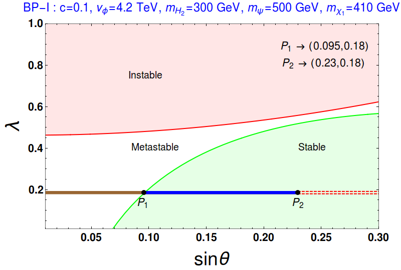
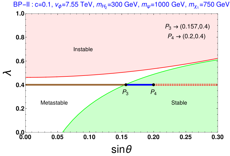
Figure 14: Vacuum stability (green), metastable (white) and instability (pink) region in $\sin\theta-\lambda$ plane for BP-I [left panel] and BP-II [right panel]. The horizontal lines describe correct relic density contours for BP-I and BP-II. The red dashed portion of these horizontal lines represent the disallowed regions from direct detection limit. The blue section of each relic contour satisfies both vacuum stability criteria as well as the direct detection bound while the brown portion is excluded by vacuum stability condition only. The points $P_{1}$ and $P_{2}$ in left panel and $P_{3}$ and $P_{4}$ from right panel will be used to show the evolution of $\lambda_{H}$ as a function of energy scale $\mu$ in Fig. 15.

In Fig.14, we constrain the $\sin\theta-\lambda$ parameter space using the absolute stability criteria ($\lambda_{H}^{\textrm{eff}}(\mu)>0$ for $\mu=m_{t}$ to $M_{P}$) for the EW vacuum for BP-I and BP-II as values of parameters given in Table 4. The solid green line in Fig. 14 indicates the boundary line in $\sin\theta-\lambda$ plane beyond which the stability criteria of SM Higgs vacuum violates. Hence all points in the green shaded region satisfies the absolute stability of the EW vacuum. Similarly the solid red line indicates the boundary of the metastable-instable region as obtained through Eq.(60). The pink shaded region therefore indicates instability of the EW vacuum with $m_{t}=173.2$ GeV and $m_{h}=125.09$ GeV. Here we use the upper limit on the scalar mixing as 0.3 so as to be consistent with experimental limits on it. The DD cross-section corresponding to these particular dark matter masses (410 GeV and 750 GeV) with specific choices of $\lambda$ ($\lambda=0.18$ in left plot while $\lambda=0.4$ in right plot in Fig. 14) against $\sin\theta$ along with the same values of other parameters ($c,v_{\phi},m_{\psi},m_{H_{2}}$) are already provided in Fig. 8 (also in Fig. 13). Using Fig. 8, we identify here the relic density satisfied contour (horizontal solid line) in the $\sin\theta-\lambda$ plane on Fig.14. We note that DD sets an upper bound on $\sin\theta$, due to which the excluded region of $\sin\theta$ is marked in red within the horizontal line(s) in both the figures. The brown portion of the $\lambda=0.18(0.4)$ line corresponds to the relic and DD allowed range of $\sin\theta$ in left(right) plot; however this falls in a region where EW vacuum is metastable. In Fig. 14 (left panel), the blue portion of the constant $\lambda$ line indicates that with this restricted region of $\sin\theta$, we have a dark matter of mass 410 GeV which satisfy the relic density and DD bounds and on the other hand, the EW vacuum remains absolutely stable all the way till $M_{P}$.

The outcome of this combined analysis of relic and DD satisfied value of a DM mass and stability of the EW vacuum in presence of two new scales, DM mass and heavy Higgs, seems to be interesting. It can significantly restrict the scalar mixing angle. For example with $m_{\chi_{1}}=410$ GeV in Fig. 8 (left panel) and $m_{H_{2}}=300$ GeV, we find $\lambda=0.18$ restricts $\sin\theta\lesssim 0.23$ which is more stringent than the existing experimental one. This set of ($\sin\theta,\lambda$) values is denoted by $P_{2}$ in left panel of

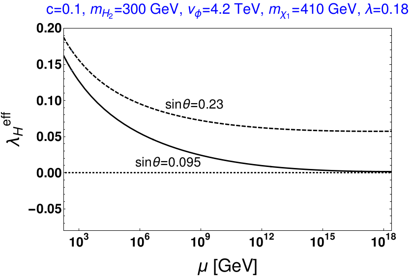
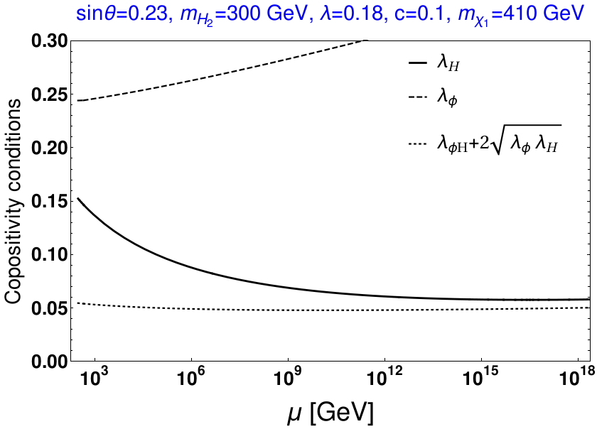
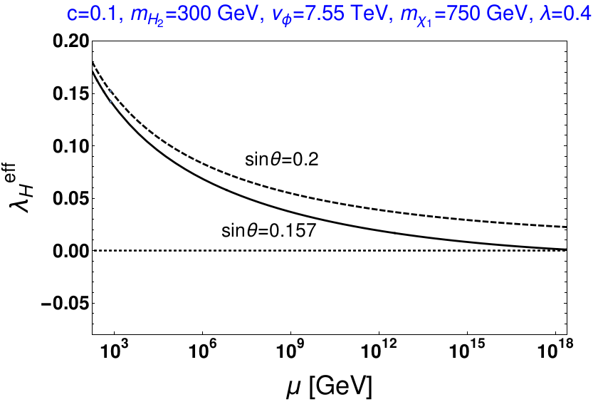
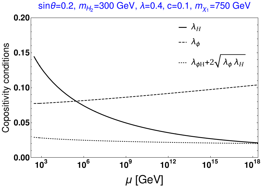
Figure 15: Evolution of $\lambda_{H}^{\textrm{eff}}$ from $\mu=m_{t}$ to $M_{P}$ for $P_{1}$, $P_{2}$ [top left] and $P_{3}$, $P_{4}$ [bottom left] points of Fig.14. In right panels, copositivity criterias are shown as a function of $\mu$ for $P_{2}$ [top] and $P_{4}$ [bottom] points.

Fig. 13. On top of this, if the EW vacuum needs to be absolutely stable, we note that we can obtain a lower limit on $\sin\theta$ as 0.095. The corresponding set of ($\sin\theta,\lambda$) values is denoted by $P_{1}$ which follows from the intersection of relic density contour ($\lambda=0.18$ line) with boundary line of the absolute stability region (solid green line). Combining these we obtain: $0.095\lesssim\sin\theta\lesssim 0.23$. A similar criteria with $m_{\chi_{1}}=750$ GeV restricts $\sin\theta$ to be within $0.157\leavevmode\nobreak\ ({\rm point\leavevmode\nobreak\ }P_{3})\lesssim\sin\theta\lesssim 0.2\leavevmode\nobreak\ ({\rm point\leavevmode\nobreak\ }P_{4})$. Therefore, from this analysis we are able to draw both upper and lower limits on $\sin\theta$ for the two benchmark points. This turns out to be the most interesting and key feature of the proposed model. The vacuum stability analysis can be extended for any other points in Fig. 13. However if we go for higher value of $\lambda$, the simultaneous satisfied region of DM relic abundance, DD cross-section bound and stability of EW vacuum will be reduced as seen while comparing the left with right panel of Fig. 14.

Finally one may wonder about the nature of evolution of $\lambda_{H}^{\textrm{eff}}$ and the co-positivity conditions for any points within EW vacuum stability satisfied region of Fig. 14. Hence, in Fig.15, running of $\lambda_{H}^{\textrm{eff}}$ is shown against the energy scale $\mu$ for $P_{1}$ and $P_{2}$ (in top left panel of Fig. 15); $P_{3}$ and $P_{4}$ (in bottom left panel of Fig. 15). Note that these two points also satisfy the relic density and DD cross-section bounds. We find for $\sin\theta=0.2$, $\lambda_{H}^{\textrm{eff}}$ remains positive starting from $\mu=m_{t}$ to $M_{P}$ energy scale and for $\sin\theta=0.157$, although $\lambda_{H}^{\textrm{eff}}$ stays positive throughout its evolution, it marginally reaches zero at $M_{P}$. Hence this point appears as the boundary point in $\sin\theta-\lambda$ plane of Fig. 14 (right panel) beyond which the SM Higgs vacuum becomes unstable. In top and bottom right panel of Fig. 15, we show the evolution of all the co-positivity conditions from $\mu=m_{t}$ to $M_{P}$ corresponding to $P_{2}$ and $P_{4}$ points respectively.

7 Conclusion

We have explored a dark matter model by extending the Standard Model of particle physics with a singlet scalar and a dark sector comprised of two Weyl doublets and a Weyl singlet fermions. The scalar singlet acquires a vev and contributes to the mass the dark sector particles consisting of three neutral Majorana fermions and one charged Dirac fermion. The lightest Majorana particle is stable due to the presence of a residual $Z_{2}$ symmetry and hence we study whether this can account for the dark matter relic density and also satisfy the direct detection bounds. There exists a mixing of the singlet scalar with the SM Higgs doublet in the model which results in two physical scalars, which in turn affect the DM phenomenology. We have found that apart from the region of two resonances, there exists a large available region of parameter space satisfying various theoretical and experimental bounds particularly due to large co-annihilations effects present. On the other hand, inclusion of new fermions in the model affects the Higgs vacuum stability adversely by leading it more toward instability at high scale due to new Yukawa like coupling. This issue however can be resolved by the involvement of extra scalar singlet. We find that with the demand of having a dark matter mass $\sim$ few hundred GeV to 1 TeV consistent with appropriate relic density and DD limits and simultaneously to make the EW vacuum absolutely stable upto the Planck scale, we can restrict the scalar mixing angle significantly. The result is carrying a strong correlation with the dark sector Yukawa coupling, $\lambda$. It turns out that, with higher dark matter mass, the allowed range of $\sin\theta$ becomes more stringent from this point of view. Hence future limits of $\sin\theta$ will have the potential to allow or rule out the model under consideration.

Acknowledgments : ADB and AS acknowledge the support from Department of Science and Technology, Government of India, under PDF/2016/002148. Work of ADB is supported by the SERB National Post-Doctoral fellowship under this project (PDF/2016/002148). AKS would like to acknowledge MHRD, Govt. of India for research fellowship. ADB and AKS also thank P. B. Pal, Anirban Biswas, Biswajit Karmakar, Rishav Roshan and Rashidul Islam for useful help and discussions.

References

- [1] G. Aad et al. [ATLAS Collaboration], Phys. Rev. D 90, no. 5, 052004 (2014) doi:10.1103/PhysRevD.90.052004 [arXiv:1406.3827 [hep-ex]].
- [2] S. Chatrchyan et al. [CMS Collaboration], JHEP 1203, 040 (2012) doi:10.1007/JHEP03(2012)040 [arXiv:1202.3478 [hep-ex]].
- [3] D. Buttazzo, G. Degrassi, P. P. Giardino, G. F. Giudice, F. Sala, A. Salvio and A. Strumia, JHEP 1312, 089 (2013) doi:10.1007/JHEP12(2013)089 [arXiv:1307.3536 [hep-ph]].
- [4] G. Degrassi, S. Di Vita, J. Elias-Miro, J. R. Espinosa, G. F. Giudice, G. Isidori and A. Strumia, JHEP 1208, 098 (2012) doi:10.1007/JHEP08(2012)098 [arXiv:1205.6497 [hep-ph]].
- [5] Y. Tang, Mod. Phys. Lett. A 28, 1330002 (2013) doi:10.1142/S0217732313300024 [arXiv:1301.5812 [hep-ph]].
- [6] J. Ellis, J. R. Espinosa, G. F. Giudice, A. Hoecker and A. Riotto, Phys. Lett. B 679, 369 (2009) doi:10.1016/j.physletb.2009.07.054 [arXiv:0906.0954 [hep-ph]].
- [7] J. Elias-Miro, J. R. Espinosa, G. F. Giudice, G. Isidori, A. Riotto and A. Strumia, Phys. Lett. B 709, 222 (2012) doi:10.1016/j.physletb.2012.02.013 [arXiv:1112.3022 [hep-ph]].
- [8] V. Khachatryan et al. [CMS Collaboration], Phys. Rev. D 93, no. 7, 072004 (2016) doi:10.1103/PhysRevD.93.072004 [arXiv:1509.04044 [hep-ex]].
- [9] G. Isidori, G. Ridolfi and A. Strumia, Nucl. Phys. B 609, 387 (2001) doi:10.1016/S0550-3213(01)00302-9 [hep-ph/0104016].
- [10] J. R. Espinosa, G. F. Giudice and A. Riotto, JCAP 0805, 002 (2008) doi:10.1088/1475-7516/2008/05/002 [arXiv:0710.2484 [hep-ph]].
- [11] O. Lebedev and A. Westphal, Phys. Lett. B 719, 415 (2013) doi:10.1016/j.physletb.2012.12.069 [arXiv:1210.6987 [hep-ph]].
- [12] A. Kobakhidze and A. Spencer-Smith, Phys. Lett. B 722, 130 (2013) doi:10.1016/j.physletb.2013.04.013 [arXiv:1301.2846 [hep-ph]].
- [13] M. Fairbairn and R. Hogan, Phys. Rev. Lett. 112, 201801 (2014) doi:10.1103/PhysRevLett.112.201801 [arXiv:1403.6786 [hep-ph]].
- [14] J. Kearney, H. Yoo and K. M. Zurek, Phys. Rev. D 91, no. 12, 123537 (2015) doi:10.1103/PhysRevD.91.123537 [arXiv:1503.05193 [hep-th]].
- [15] A. Hook, J. Kearney, B. Shakya and K. M. Zurek, JHEP 1501, 061 (2015) doi:10.1007/JHEP01(2015)061 [arXiv:1404.5953 [hep-ph]].
- [16] P. Ghosh, A. K. Saha and A. Sil, Phys. Rev. D 97, no. 7, 075034 (2018) doi:10.1103/PhysRevD.97.075034 [arXiv:1706.04931 [hep-ph]].
- [17] D. S. Akerib et al. [LUX Collaboration], Phys. Rev. Lett. 118, no. 2, 021303 (2017) doi:10.1103/PhysRevLett.118.021303 [arXiv:1608.07648 [astro-ph.CO]].
- [18] E. Aprile et al. [XENON Collaboration], Phys. Rev. Lett. 119, no. 18, 181301 (2017) doi:10.1103/PhysRevLett.119.181301 [arXiv:1705.06655 [astro-ph.CO]].
- [19] X. Cui et al. [PandaX-II Collaboration], Phys. Rev. Lett. 119, no. 18, 181302 (2017) doi:10.1103/PhysRevLett.119.181302 [arXiv:1708.06917 [astro-ph.CO]].
- [20] E. Aprile et al. [XENON Collaboration], JCAP 1604, no. 04, 027 (2016) doi:10.1088/1475-7516/2016/04/027 [arXiv:1512.07501 [physics.ins-det]].
- [21] I. Gogoladze, N. Okada and Q. Shafi, Phys. Rev. D 78, 085005 (2008) doi:10.1103/PhysRevD.78.085005 [arXiv:0802.3257 [hep-ph]].
- [22] J. Elias-Miro, J. R. Espinosa, G. F. Giudice, H. M. Lee and A. Strumia, JHEP 1206, 031 (2012) doi:10.1007/JHEP06(2012)031 [arXiv:1203.0237 [hep-ph]].
- [23] O. Lebedev, Eur. Phys. J. C 72, 2058 (2012) doi:10.1140/epjc/s10052-012-2058-2 [arXiv:1203.0156 [hep-ph]].
- [24] N. Khan and S. Rakshit, Phys. Rev. D 90, no. 11, 113008 (2014) doi:10.1103/PhysRevD.90.113008 [arXiv:1407.6015 [hep-ph]].
- [25] V. V. Khoze, C. McCabe and G. Ro, JHEP 1408, 026 (2014) doi:10.1007/JHEP08(2014)026 [arXiv:1403.4953 [hep-ph]].
- [26] M. Gonderinger, Y. Li, H. Patel and M. J. Ramsey-Musolf, JHEP 1001, 053 (2010) doi:10.1007/JHEP01(2010)053 [arXiv:0910.3167 [hep-ph]].
- [27] I. Garg, S. Goswami, Vishnudath K.N. and N. Khan, Phys. Rev. D 96, no. 5, 055020 (2017) doi:10.1103/PhysRevD.96.055020 [arXiv:1706.08851 [hep-ph]].
- [28] C. S. Chen and Y. Tang, JHEP 1204, 019 (2012) doi:10.1007/JHEP04(2012)019 [arXiv:1202.5717 [hep-ph]].
- [29] N. Chakrabarty, U. K. Dey and B. Mukhopadhyaya, JHEP 1412, 166 (2014) doi:10.1007/JHEP12(2014)166 [arXiv:1407.2145 [hep-ph]].
- [30] N. Chakrabarty, D. K. Ghosh, B. Mukhopadhyaya and I. Saha, Phys. Rev. D 92, no. 1, 015002 (2015) doi:10.1103/PhysRevD.92.015002 [arXiv:1501.03700 [hep-ph]].
- [31] N. Chakrabarty and B. Mukhopadhyaya, Eur. Phys. J. C 77, no. 3, 153 (2017) doi:10.1140/epjc/s10052-017-4705-0 [arXiv:1603.05883 [hep-ph]].
- [32] R. Costa, A. P. Morais, M. O. P. Sampaio and R. Santos, Phys. Rev. D 92, 025024 (2015) doi:10.1103/PhysRevD.92.025024 [arXiv:1411.4048 [hep-ph]].
- [33] S. Oda, N. Okada and D. s. Takahashi, Phys. Rev. D 96, no. 9, 095032 (2017) doi:10.1103/PhysRevD.96.095032 [arXiv:1704.05023 [hep-ph]].
- [34] K. Bhattacharya, J. Chakrabortty, S. Das and T. Mondal, JCAP 1412, no. 12, 001 (2014) doi:10.1088/1475-7516/2014/12/001 [arXiv:1408.3966 [hep-ph]].
- [35] A. K. Saha and A. Sil, Phys. Lett. B 765, 244 (2017) doi:10.1016/j.physletb.2016.12.031 [arXiv:1608.04919 [hep-ph]].
- [36] S. Oda, N. Okada, D. Raut and D. s. Takahashi, Phys. Rev. D 97, no. 5, 055001 (2018) doi:10.1103/PhysRevD.97.055001 [arXiv:1711.09850 [hep-ph]].
- [37] A. Datta, A. Elsayed, S. Khalil and A. Moursy, Phys. Rev. D 88, no. 5, 053011 (2013) doi:10.1103/PhysRevD.88.053011 [arXiv:1308.0816 [hep-ph]].
- [38] C. Coriano, L. Delle Rose and C. Marzo, Phys. Lett. B 738, 13 (2014) doi:10.1016/j.physletb.2014.09.001 [arXiv:1407.8539 [hep-ph]].
- [39] J. N. Ng and A. de la Puente, Eur. Phys. J. C 76, no. 3, 122 (2016) doi:10.1140/epjc/s10052-016-3981-4 [arXiv:1510.00742 [hep-ph]].
- [40] C. Bonilla, R. M. Fonseca and J. W. F. Valle, Phys. Lett. B 756, 345 (2016) doi:10.1016/j.physletb.2016.03.037 [arXiv:1506.04031 [hep-ph]].
- [41] N. Haba and Y. Yamaguchi, PTEP 2015, no. 9, 093B05 (2015) doi:10.1093/ptep/ptv121 [arXiv:1504.05669 [hep-ph]].
- [42] J. Chakrabortty, P. Konar and T. Mondal, Phys. Rev. D 89, no. 5, 056014 (2014) doi:10.1103/PhysRevD.89.056014 [arXiv:1308.1291 [hep-ph]].
- [43] S. Khan, S. Goswami and S. Roy, Phys. Rev. D 89, no. 7, 073021 (2014) doi:10.1103/PhysRevD.89.073021 [arXiv:1212.3694 [hep-ph]].
- [44] C. Cai, Z. H. Yu and H. H. Zhang, Nucl. Phys. B 921, 181 (2017) doi:10.1016/j.nuclphysb.2017.05.015 [arXiv:1611.02186 [hep-ph]].
- [45] R. Mahbubani and L. Senatore, Phys. Rev. D 73, 043510 (2006) doi:10.1103/PhysRevD.73.043510 [hep-ph/0510064].
- [46] F. D’Eramo, Phys. Rev. D 76, 083522 (2007) doi:10.1103/PhysRevD.76.083522 [arXiv:0705.4493 [hep-ph]].
- [47] R. Enberg, P. J. Fox, L. J. Hall, A. Y. Papaioannou and M. Papucci, JHEP 0711, 014 (2007) doi:10.1088/1126-6708/2007/11/014 [arXiv:0706.0918 [hep-ph]].
- [48] T. Cohen, J. Kearney, A. Pierce and D. Tucker-Smith, Phys. Rev. D 85, 075003 (2012) doi:10.1103/PhysRevD.85.075003 [arXiv:1109.2604 [hep-ph]].
- [49] C. Cheung and D. Sanford, JCAP 1402, 011 (2014) doi:10.1088/1475-7516/2014/02/011 [arXiv:1311.5896 [hep-ph]].
- [50] L. Calibbi, A. Mariotti and P. Tziveloglou, JHEP 1510, 116 (2015) doi:10.1007/JHEP10(2015)116 [arXiv:1505.03867 [hep-ph]].
- [51] S. Horiuchi, O. Macias, D. Restrepo, A. Rivera, O. Zapata and H. Silverwood, JCAP 1603, no. 03, 048 (2016) doi:10.1088/1475-7516/2016/03/048 [arXiv:1602.04788 [hep-ph]].
- [52] S. Banerjee, S. Matsumoto, K. Mukaida and Y. L. S. Tsai, JHEP 1611, 070 (2016) doi:10.1007/JHEP11(2016)070 [arXiv:1603.07387 [hep-ph]].
- [53] T. Abe, Phys. Lett. B 771, 125 (2017) doi:10.1016/j.physletb.2017.05.048 [arXiv:1702.07236 [hep-ph]].
- [54] Q. F. Xiang, X. J. Bi, P. F. Yin and Z. H. Yu, Phys. Rev. D 97, no. 5, 055004 (2018) doi:10.1103/PhysRevD.97.055004 [arXiv:1707.03094 [hep-ph]].
- [55] N. Maru, T. Miyaji, N. Okada and S. Okada, JHEP 1707, 048 (2017) doi:10.1007/JHEP07(2017)048 [arXiv:1704.04621 [hep-ph]].
- [56] N. Maru, N. Okada and S. Okada, Phys. Rev. D 96, no. 11, 115023 (2017) doi:10.1103/PhysRevD.96.115023 [arXiv:1801.00686 [hep-ph]].
- [57] L. Calibbi, L. Lopez-Honorez, S. Lowette and A. Mariotti, arXiv:1805.04423 [hep-ph].
- [58] S. Esch, M. Klasen and C. E. Yaguna, arXiv:1804.03384 [hep-ph].
- [59] G. Arcadi, arXiv:1804.04930 [hep-ph].
- [60] N. Arkani-Hamed, A. Delgado and G. F. Giudice, Nucl. Phys. B 741, 108 (2006).
- [61] S. Bhattacharya, B. Karmakar, N. Sahu and A. Sil, Phys. Rev. D 93, no. 11, 115041 (2016) doi:10.1103/PhysRevD.93.115041 [arXiv:1603.04776 [hep-ph]].
- [62] S. Bhattacharya, B. Karmakar, N. Sahu and A. Sil, JHEP 1705, 068 (2017) doi:10.1007/JHEP05(2017)068 [arXiv:1611.07419 [hep-ph]].
- [63] S. Bhattacharya, N. Sahoo and N. Sahu, Phys. Rev. D 96, no. 3, 035010 (2017) doi:10.1103/PhysRevD.96.035010 [arXiv:1704.03417 [hep-ph]].
- [64] S. Bhattacharya, N. Sahoo and N. Sahu, Phys. Rev. D 93, no. 11, 115040 (2016) doi:10.1103/PhysRevD.93.115040 [arXiv:1510.02760 [hep-ph]].
- [65] N. Narendra, N. Sahoo and N. Sahu, arXiv:1712.02960 [hep-ph].
- [66] C. E. Yaguna, Phys. Rev. D 92, no. 11, 115002 (2015) doi:10.1103/PhysRevD.92.115002 [arXiv:1510.06151 [hep-ph]].
- [67] C. Fu et al. [PandaX-II Collaboration], Phys. Rev. Lett. 118, no. 7, 071301 (2017) doi:10.1103/PhysRevLett.118.071301 [arXiv:1611.06553 [hep-ex]].
- [68] D. Egana-Ugrinovic, JHEP 1712, 064 (2017) doi:10.1007/JHEP12(2017)064 [arXiv:1707.02306 [hep-ph]].
- [69] B. Adhikary, M. Chakraborty and A. Ghosal, JHEP 1310, 043 (2013) Erratum: [JHEP 1409, 180 (2014)] doi:10.1007/JHEP10(2013)043, 10.1007/JHEP09(2014)180 [arXiv:1307.0988 [hep-ph]].
- [70] S. P. Martin, Adv. Ser. Direct. High Energy Phys. 21, 1 (2010) [Adv. Ser. Direct. High Energy Phys. 18, 1 (1998)] [hep-ph/9709356].
- [71] C. Patrignani et al. [Particle Data Group], Chin. Phys. C 40, no. 10, 100001 (2016). doi:10.1088/1674-1137/40/10/100001
- [72] T. Robens and T. Stefaniak, Eur. Phys. J. C 75, 104 (2015) doi:10.1140/epjc/s10052-015-3323-y [arXiv:1501.02234 [hep-ph]].
- [73] G. Chalons, D. Lopez-Val, T. Robens and T. Stefaniak, PoS DIS 2016, 113 (2016) [arXiv:1606.07793 [hep-ph]].
- [74] T. Robens and T. Stefaniak, Eur. Phys. J. C 76, no. 5, 268 (2016) doi:10.1140/epjc/s10052-016-4115-8 [arXiv:1601.07880 [hep-ph]].
- [75] K. Kannike, Eur. Phys. J. C 72, 2093 (2012) doi:10.1140/epjc/s10052-012-2093-z [arXiv:1205.3781 [hep-ph]].
- [76] J. Chakrabortty, P. Konar and T. Mondal, Phys. Rev. D 89, no. 9, 095008 (2014) doi:10.1103/PhysRevD.89.095008 [arXiv:1311.5666 [hep-ph]].
- [77] J. Horejsi and M. Kladiva, Eur. Phys. J. C 46, 81 (2006) doi:10.1140/epjc/s2006-02472-3 [hep-ph/0510154].
- [78] G. Bhattacharyya and D. Das, Pramana 87, no. 3, 40 (2016) doi:10.1007/s12043-016-1252-4 [arXiv:1507.06424 [hep-ph]].
- [79] S. K. Kang and J. Park, JHEP 1504, 009 (2015) doi:10.1007/JHEP04(2015)009 [arXiv:1306.6713 [hep-ph]].
- [80] S. Schael et al. [ALEPH and DELPHI and L3 and OPAL and SLD Collaborations and LEP Electroweak Working Group and SLD Electroweak Group and SLD Heavy Flavour Group], Phys. Rept. 427, 257 (2006) doi:10.1016/j.physrep.2005.12.006 [hep-ex/0509008].
- [81] CMS Collaboration [CMS Collaboration], CMS-PAS-HIG-16-016.
- [82] D. López-Val and T. Robens, Phys. Rev. D 90, 114018 (2014) doi:10.1103/PhysRevD.90.114018 [arXiv:1406.1043 [hep-ph]].
- [83] M. J. Strassler and K. M. Zurek, Phys. Lett. B 661, 263 (2008) doi:10.1016/j.physletb.2008.02.008 [hep-ph/0605193].
- [84] V. Khachatryan et al. [CMS Collaboration], JHEP 1510, 144 (2015) doi:10.1007/JHEP10(2015)144 [arXiv:1504.00936 [hep-ex]].
- [85] G. Aad et al. [ATLAS Collaboration], Eur. Phys. J. C 76, no. 1, 45 (2016) doi:10.1140/epjc/s10052-015-3820-z [arXiv:1507.05930 [hep-ex]].
- [86] S. Chatrchyan et al. [CMS Collaboration], Phys. Rev. D 89, no. 9, 092007 (2014) doi:10.1103/PhysRevD.89.092007 [arXiv:1312.5353 [hep-ex]].
- [87] CMS Collaboration (2012), CMS-PAS-HIG-12-045.
- [88] CMS Collaboration (2013), CMS-PAS-HIG-13-003.
- [89] ATLAS and CMS Collaborations (2015), ATLAS-CONF-2015-044
- [90] J. Abdallah et al. [DELPHI Collaboration], interpretation of the results within the MSSM,” Eur. Phys. J. C 31, 421 (2003) doi:10.1140/epjc/s2003-01355-5 [hep-ex/0311019].
- [91] M. E. Peskin and T. Takeuchi, Phys. Rev. D 46, 381 (1992). doi:10.1103/PhysRevD.46.381
- [92] V. Barger, P. Langacker, M. McCaskey, M. J. Ramsey-Musolf and G. Shaughnessy, Phys. Rev. D 77, 035005 (2008) doi:10.1103/PhysRevD.77.035005 [arXiv:0706.4311 [hep-ph]].
- [93] S. Ghosh, A. Kundu and S. Ray, Phys. Rev. D 93, no. 11, 115034 (2016) doi:10.1103/PhysRevD.93.115034 [arXiv:1512.05786 [hep-ph]].
- [94] R. Barbieri, L. J. Hall, Y. Nomura and V. S. Rychkov, Phys. Rev. D 75, 035007 (2007) doi:10.1103/PhysRevD.75.035007 [hep-ph/0607332].
- [95] J. McDonald, Phys. Rev. D 50, 3637 (1994) doi:10.1103/PhysRevD.50.3637 [hep-ph/0702143 [HEP-PH]].
- [96] G. Cynolter and E. Lendvai, Eur. Phys. J. C 58, 463 (2008)
- [97] P. A. R. Ade et al. [Planck Collaboration], Astron. Astrophys. 594, A13 (2016) doi:10.1051/0004-6361/201525830 [arXiv:1502.01589 [astro-ph.CO]].
- [98] E. Gabrielli, M. Heikinheimo, K. Kannike, A. Racioppi, M. Raidal and C. Spethmann, Phys. Rev. D 89, no. 1, 015017 (2014) doi:10.1103/PhysRevD.89.015017 [arXiv:1309.6632 [hep-ph]].
- [99] L. Lopez-Honorez, T. Schwetz and J. Zupan, Phys. Lett. B 716, 179 (2012) doi:10.1016/j.physletb.2012.07.017 [arXiv:1203.2064 [hep-ph]].
- [100] J. M. Alarcon, J. Martin Camalich and J. A. Oller, Phys. Rev. D 85, 051503 (2012) doi:10.1103/PhysRevD.85.051503 [arXiv:1110.3797 [hep-ph]].
- [101] J. M. Alarcon, L. S. Geng, J. Martin Camalich and J. A. Oller, Phys. Lett. B 730, 342 (2014) doi:10.1016/j.physletb.2014.01.065 [arXiv:1209.2870 [hep-ph]].
- [102] P. Agrawal, Z. Chacko, C. Kilic and R. K. Mishra, arXiv:1003.1912 [hep-ph].
- [103] A. Semenov, Comput. Phys. Commun. 201, 167 (2016) doi:10.1016/j.cpc.2016.01.003 [arXiv:1412.5016 [physics.comp-ph]].
- [104] G. Belanger, F. Boudjema, A. Pukhov and A. Semenov, Comput. Phys. Commun. 185, 960 (2014) doi:10.1016/j.cpc.2013.10.016 [arXiv:1305.0237 [hep-ph]].
- [105] Q. Lu, D. E. Morrissey and A. M. Wijangco, JHEP 1706, 138 (2017) doi:10.1007/JHEP06(2017)138 [arXiv:1705.08896 [hep-ph]].
- [106] L. N. Mihaila, J. Salomon and M. Steinhauser, Phys. Rev. Lett. 108, 151602 (2012) doi:10.1103/PhysRevLett.108.151602 [arXiv:1201.5868 [hep-ph]].
- [107] L. Mihaila, J. Salomon and M. Steinhauser, PoS LL 2012, 043 (2012) [PoS LL 2012, 043 (2012)] [arXiv:1209.5497 [hep-ph]].
- [108] A. V. Bednyakov, A. F. Pikelner and V. N. Velizhanin, Phys. Lett. B 722, 336 (2013) doi:10.1016/j.physletb.2013.04.038 [arXiv:1212.6829 [hep-ph]].
- [109] J. A. Casas, J. R. Espinosa and M. Quiros, Phys. Lett. B 342, 171 (1995) doi:10.1016/0370-2693(94)01404-Z [hep-ph/9409458].