Percolation Thresholds and Fisher Exponents in Hypercubic Lattices

Abstract

We use invasion percolation to compute highly accurate numerical values for bond and site percolation thresholds $p_{c}$ on the hypercubic lattice $\mathbb{Z}^{d}$ for $d=4,\ldots,13$. We also compute the Fisher exponent $\tau$ governing the cluster size distribution at criticality. Our results support the claim that the mean-field value $\tau=5/2$ holds for $d\geq 6$, with logarithmic corrections to power-law scaling at $d=6$.

I Introduction

According to Auguste Rodin, “sculpture is the art of the hole and the lump” Mauclair (1905). Percolation is the science of the hole and the lump: each site of a lattice is considered a lump with probability $p$ and a hole with probability $1-p$. Lumps that are connected to each other form larger lumps, and in percolation theory Grimmett (1999); *stauffer:aharony:book one studies the structure of these large lumps as a function of $p$.

Whereas the sculptor is confined to three-dimensional pieces of art, the scientist can study structures in any dimension. In this contribution we study percolation on the hypercubic lattce $\mathbb{Z}^{d}$ in dimensions $d=4,\ldots,13$. In particular we present a method that allows us to approximate the critical density $p_{c}$ very efficiently. This is the density at which a lump—pardon, a cluster—first appears that spans the entire system.

For larger values of $d$, numerical simulations in $\mathbb{Z}^{d}$ are challenging because the lattice quickly becomes too big to fit into the memory of a computer. Grassberger Grassberger (2003) avoided this problem by growing single clusters at a given value of $p$ using the Leath algorithm Leath (1976a). With this approach, he estimated the critical densities to 5 or 6 digits of accuracy. We will use another algorithm—invasion percolation—to get even more accurate estimates of the critical densities.

The paper is organized as follows. We begin by explaining the basic invasion percolation algorithm and its efficient implementation for percolation on $\mathbb{Z}^{d}$. In Section III we discuss how to compute $p_{c}$ from simple properties of the invasion cluster. Section IV provides our numerical results, including our new estimates of $p_{c}$ and how they compare to previous results. In Sections V and VI we examine the scaling of the cluster size distribution, and to what extent it supports the claim that $d=6$ is the upper critical dimension. We find that the Fisher exponent $\tau$ matches its mean-field value $5/2$ for $d\geq 6$, with logarithmic corrections at $d=6$.

II Invasion Percolation

Invasion percolation is a stochastic growth process that was introduced as a model of fluid transport through porous media Lenormand and Bories (1980); Chandler et al. (1982); Wilkinson and Willemsen (1983). It starts with a single seed vertex of the underlying graph, and grows a cluster around it. There are two versions of the model which invade vertices or edges, which we use to study site and bond percolation respectively. For site percolation, we assign each vertex a random weight uniformly distributed in the unit interval $[0,1]$. At each step, we add the neighboring vertex with the smallest weight to the cluster, increasing the cluster size $N$ by one. For bond percolation, we assign weights to edges rather than vertices, and we extend the invasion cluster along the edge incident to it with the smallest weight. For simplicity, we will focus our discussion here on site percolation.

The benefit of invasion percolation is that we do not need to store a lattice large enough to hold the largest cluster that we might encounter; for high-dimensional lattices this would be computationally infeasible. Instead we only need to store the vertices belonging to the cluster, and the weights of the neighboring sites, which we can choose “on the fly” as the cluster grows. Because the coordination number of the lattice is fixed, the total number of vertices and weights we need to store grows only linearly with the mass of the cluster.

We use two data structures to keep track of the vertices we have explored so far, and to find the boundary vertex with the smallest weight. A set is used to hold all vertices that have already been assigned weights, and a priority queue Dasgupta et al. (2006) is used to hold the boundary, i.e., all vertices that have been assigned weights that are not already part of the cluster. The priority queue lets us select and remove the lowest-weight vertex from the boundary, or add new vertices to it, in time logarithmic in the size of the boundary. The set lets us add, remove, or search for a vertex in a cluster of size $N$ in time $O(\log N)$. Thus each step of invasion percolation takes $O(\log N)$ time.

Modern programming languages provide built-in implementations of these data structures, such as the container classes set and priority_queue from the C++ standard library Weert and Gregoire (2016). While these implementations are convenient, we found it more efficient to build our own implementation of the set data structure as a hash table, using essentially the same hash function as in Grassberger (2003).

A priori, invasion percolation differs from classical Bernoulli percolation, where each vertex is independently occupied with probability $p$. But invasion percolation reproduces, both qualitatively and quantitatively, Bernoulli percolation at criticality Chayes et al. (1985); Häggström et al. (1999). We can explain this connection as follows. Since the vertex weights are uniform in the unit interval, one way to implement Bernoulli percolation is to declare a vertex occupied if its weight is less than $p$. If $p>p_{c}$, the occupied sites possess a unique infinite component. If the initial vertex is in a finite component, invasion percolation fills it and then breaks out of it by adding a vertex with weight greater than $p$; but after an initial transient of these finite components, it breaks through to the infinite component. After that, it grows the cluster to infinite mass by adding vertices of weight less than $p$.

Thus, for any $p>p_{c}$, the maximum weight of the vertices added to the cluster falls below $p$ after some finite time. As the cluster grows, the maximum weight approaches $p_{c}$ from above, so the weights of the vertices added to the cluster are asymptotically uniform in the interval $[0,p_{c}]$.

III Measuring the Threshold

To compute $p_{c}$ using invasion percolation, we use a simple estimator. Let $B(N)$ denote the number of vertices that have been assigned weights in the course of building a cluster with mass $N$, i.e., which are either in the cluster or on its boundary. Since almost all of the $N$ vertices actually added to the cluster have weight less than or equal to $p_{c}$, and since the weight distribution is uniform, we have

$$\lim_{N\to\infty}\frac{N}{B(N)}=p_{c}\,.$$ (1)

The relationship between $p_{c}$ and this “boundary-to-bulk ratio” goes back to the classic work of Leath Leath (1976a). The limit (1) has been established rigorously for invasion bond percolation in $\mathbb{Z}^{2}$ Chayes et al. (1985), but it is believed to hold on general lattices. Moreover, it appears to be an excellent numerical estimator for $p_{c}$, and in Mertens and Moore (2017) we used it to estimate $p_{c}$ to high precision on hyperbolic lattices.

Based on these facts, we estimate $p_{c}$ by extrapolating the measured values $N/B(N)$ to $N=\infty$. The estimator $N/B(N)$ is extremely easy to compute, since $N$ and $B(N)$ are simply integers given by the progress of the invasion percolation process. Moreover, it turns out to have excellent finite-size scaling and small statistical fluctuations.

We first consider the behavior of this estimator on a Bethe lattice of degree $\Delta$, i.e., a tree where every vertex has $\Delta-1$ children. Here we have $p_{c}=1/(\Delta-1)$ for both site and bond percolation. Moreover, any cluster of mass $N$ is surrounded by exactly $(\Delta-2)N+2$ neighboring vertices regardless of its shape, giving

$$\frac{N}{B(N)}=\frac{N}{(\Delta-1)N+2}=\frac{p_{c}}{1+\frac{2}{(\Delta-1)N}}\,.$$ (2)

Thus on the tree this estimator has zero variance, and a finite-size effect which decays as $O(N^{-\delta})$ for $\delta=1$.

We find that the convergence of this estimator is almost as good on $d$-dimensional lattices as it is on the tree. As in Mertens and Moore (2017) we assume the form

$$\frac{N}{B(N)}=\frac{p_{c}}{1+bN^{-\delta}}\simeq p_{c}(1-bN^{-\delta})$$ (3)

and fit the parameters $p_{c}$, $b$, and $\delta$ to our numerical data. We will see that $\delta$ quickly approaches $1$ as $d$ increases. This is plausible since high-dimensional lattices are treelike, in the sense that most paths never return to the origin. Moreover, $N/B(N)$ has small statistical fluctuations, so we can obtain accurate estimates of $p_{c}$ with a reasonable number of independent runs of the algorithm.

It is interesting to consider the relationship between $\delta$ and the transient described above. The invasion cluster of mass $N$ contains both “good” vertices, i.e., those with weights in the interval $[0,p_{c}]$, and “breakout” vertices of weight greater than $p_{c}$, which are added to the cluster whenever it fills a finite component and runs out of good vertices on the boundary. One might think that the error in the estimator comes from these breakout vertices: for instance, one might think that if there are $N_{b}=O(N^{\alpha})$ breakout vertices in the cluster, then the error is $O(N_{b}/N)=O(N^{-\delta})$ where $\delta=1-\alpha$.

However, this is overly pessimistic. On the tree, each boundary vertex has $\Delta-1$ children; the probability that a given child is good is $p_{c}=1/(\Delta-1)$, so the expected number of good children is $1$. Since invasion percolation will add a good boundary vertex to the cluster if there is one, it follows that the number $N_{g}$ of good boundary vertices follows an unbiased random walk. A breakout occurs when $N_{g}=0$, i.e., when this random walk touches the origin. Since an unbiased random walk touches the origin $O(N^{1/2})$ times in its first $N$ steps, the cluster includes $N_{b}=O(N^{1/2})$ breakout vertices. On the other hand, after $N$ steps there are also typically $N_{g}=O(N^{1/2})$ good vertices waiting to be added to the cluster. Miraculously, these two cancel out, and $N=p_{c}B(N)+O(1)$ as shown in (2). We suspect that a similar cancellation occurs on lattices, so that $\delta$ is smaller than one would expect from naively considering the number of breakouts before the infinite component is reached.

IV Critical Densities

To compute $p_{c}$ numerically, we grow an invasion cluster and report values of $N/B(N)$ for

$$N=\lfloor 100\times 2^{t/4}\rfloor\qquad(t=0,1,\ldots,67)\,,$$ (4)

where $\lfloor x\rfloor$ denotes the integer part of $x$. This correponds to cluster sizes ranging from $100$ to $\numprint{11021797}\approx 10^{7}$. These $68$ data points are then averaged over $10^{6}$ independent runs of the invasion percolation algorithm. Figure 1 shows that the statistical fluctuations between runs are small: for large $d$ the standard deviation decays as $O(N^{-1/2})$, just as if the $N$ steps of invasion percolation were independent events.

The data follows (3) very well, as can be seen from Figure 2. Fitting $p_{c}$, $b$, and $\delta$, and thus extrapolating $N/B(N)$ to $N\to\infty$, then allows us to estimate $p_{c}$. Table 1 shows that the exponent $\delta$ governing the finite-size effects increases with $d$, approaching its treelike value $1$. Together with the small standard deviation of $B(N)/N$, these values of $N$ and the sample size of $10^{6}$ are large enough to estimate $p_{c}$ quite precisely.

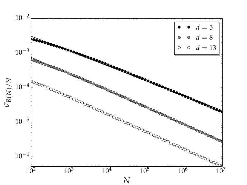
Figure 1: The standard deviation of $B(N)/N$ vs. $N$ over multiple runs of invasion percolation. The straight lines show that the statistical fluctuations decay as $O(N^{-1/2})$ for large $d$. For $d=5$ the decay is slightly slower, $O(N^{-0.46})$.

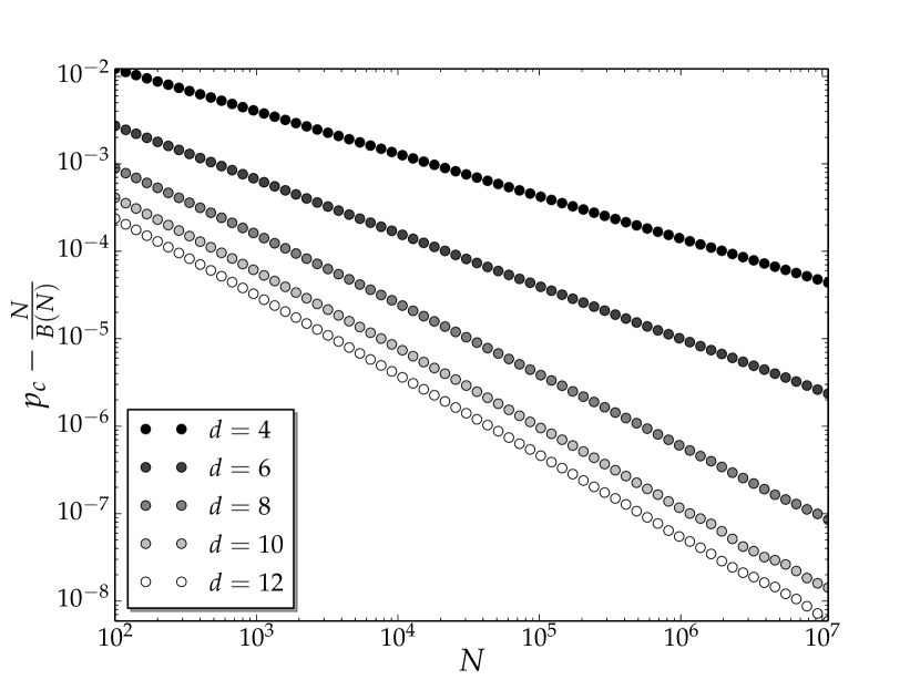
Figure 2: Convergence of $N/B(N)$ to $p_{c}^{\text{site}}$. The finite-size effects decay as $O(N^{-\delta})$, where $\delta$ approaches $1$ for large $d$.

$\begin{array}[]{ll}d&\delta\\ \hline\cr 4&0.483\,21(6)\\ 5&0.518\,3(3)\\ 6&0.601\,2(3)\\ 7&0.717\,9(4)\\ 8&0.812(1)\\ 9&0.870(2)\\ 10&0.903(2)\\ 11&0.911(1)\\ 12&0.916(1)\\ 13&0.935(1)\end{array}$

Table 1: Numerical values of the exponent $\delta$ governing the finite-size effects (3). As $d$ increases, $\delta$ approaches its value $1$ on the tree.

Table 2 contains the values for $p_{c}$ obtained by our approach, for both site and bond percolation, in comparison to the most precise values we could find in the literature. Our values for $p_{c}$ are consistent with the previous results of Grassberger (2003); Dammer and Hinrichsen (2004) but are more accurate. Note that, because $\delta$ increases with $d$, our estimates become more accurate as $d$ increases: with invasion clusters of size $N=10^{7}$, our multiplicative error on $p_{c}$ is $10^{-4}$ for $d=4$, but just $10^{-8}$ for $d=13$. Our new values have error bars that are at least a factor $10^{-2}$ smaller than those of the previous values, giving $p_{c}$ to two or three more digits of accuracy.

$d$	$p_{c}^{\text{site}}$	$p_{c}^{\text{bond}}$
4	0.196 886 1(14)Grassberger (2003)	0.160 131 0(10)Dammer and Hinrichsen (2004)
	0.196 885 61(3)	0.160 131 22(6)
5	0.140 796 6(15)Grassberger (2003)	0.118 171 8(3)Dammer and Hinrichsen (2004)
	0.140 796 33(4)	0.118 171 45(3)
6	0.109 017(2)Grassberger (2003)	0.094 201 9(6)Grassberger (2003)
	0.109 016 661(8)	0.094 201 65(2)
7	0.088 951 1(9)Grassberger (2003)	0.078 675 2(3)Grassberger (2003)
	0.088 951 121(1)	0.078 675 230(2)
8	0.075 210 1(5)Grassberger (2003)	0.067 708 39(7)Grassberger (2003)
	0.075 210 128(1)	0.067 708 418 1(3)
9	0.065 209 5(3)Grassberger (2003)	0.059 496 01(5)Grassberger (2003)
	0.065 209 5348(6)	0.059 496 003 4(1)
10	0.057 593 0(1)Grassberger (2003)	0.053 092 58(4)Grassberger (2003)
	0.057 592 948 8(4)	0.053 092 584 2(2)
11	0.051 589 71(8)Grassberger (2003)	0.047 949 69(1)Grassberger (2003)
	0.051 589 684 3(2)	0.047 949 683 73(8)
12	0.046 730 99(6)Grassberger (2003)	0.043 723 86(1)Grassberger (2003)
	0.046 730 975 5(1)	0.043 723 858 25(10)
13	0.042 715 08(8)Grassberger (2003)	0.040 187 62(1)Grassberger (2003)
	0.042 715 079 60(10)	0.040 187 617 03(6)

Table 2: Previous and new numerical values for the percolation thresholds on the $d$-dimensional hypercube.

V Fisher Exponent $\mathbf{\tau}$

Now that we have precise values for $p_{c}$, we can measure other quantities at criticality, such as the cluster size distribution and critical exponents. According to scaling theory, the average number of clusters of size $s$ per lattice site scales as

$$n_{s}(p)=s^{-\tau}\,(f_{0}(z)+s^{-\Omega}f_{1}(z)+\cdots)\,,$$ (5)

where the exponent $\Omega$ governs the leading finite-size corrections (e.g. Ziff (2011)). The scaling functions $f_{0}$ and $f_{1}$ are analytic for small values of $z$, and where the scaling variable $z$ is defined as

$$z=(p-p_{c})s^{\sigma}\,.$$ (6)

(We ignore nonuniversal metric factors in $z$.) At $p=p_{c}$ we have $z=0$, and (5) becomes

$$n_{s}(p_{c})=s^{-\tau}\,(c_{0}+c_{1}s^{-\Omega}+\cdots)\,,$$ (7)

for some constants $c_{0}=f_{0}(0)$ and $c_{1}=f_{1}(0)$.

The critical exponents $\tau$ and $\sigma$ are known exactly for percolation in two dimensions from conformal field theory and exactly solvable models (e.g. Nienhuis et al. (1980)), and on the Bethe lattice from mean field theory:

$$(\tau,\sigma)=\begin{cases}\left(\frac{187}{91},\frac{36}{91}\right)&d=2\,,\\ \left(\frac{5}{2},\frac{1}{2}\right)&\mbox{Bethe lattice.}\end{cases}$$ (8)

It is believed that upper critical dimension for percolation is $d_{c}=6$, i.e., that $\tau$ and $\sigma$ take their mean-field values for $d\geq d_{c}$. The original argument by Toulouse Toulouse (1974) rests on the Josephson hyper-scaling relation

$$d\nu=2\beta+\gamma\,,$$ (9)

that relates the critical exponents $\nu$, $\beta$, and $\gamma$ with the spatial dimension $d$. For the mean-field solution on the Bethe lattice we have $\beta=\gamma=1$ and $\nu=\frac{1}{2}$, which implies $d_{c}=6$. Rigorous results provide only upper bounds for the critical dimension; the best known bounds are $6\leq d_{c}\leq 10$ Chayes and Chayes (1987); Fitzner and van der Hofstad (2017). We will compute $\tau$ numerically for $3\leq d\leq 10$ and see that these values support the claim that $d_{c}=6$, with logarithmic corrections at $d=d_{c}$.

To measure the critical exponent $\tau$, we grow a cluster outward from the origin using the Leath algorithm Leath (1976a); *leath:76b. This is similar to invasion percolation except that it adds every neighboring vertex with weight $p\leq p_{c}$ to the cluster, instead of just the vertex with minimum weight. By running the Leath algorithm $T$ times at $p=p_{c}$, we generate $T$ independent samples from the cluster size distribution at criticality. The probability $P(s)$ that a given occupied vertex is contained in a cluster of size $s$ scales as $sn_{s}\sim s^{-(\tau-1)}$, so we can infer $\tau$ from the fraction $T_{s}/T$ of runs in which the Leath algorithm gives a cluster of each size $s$.

We fit $\tau$ to the data from these experiments using the complementary cumulative distribution $Q(s)=\sum_{s^{\prime}=s}^{\infty}P(s^{\prime})$. Including the term of (7) governing the leading finite-size effects and approximating this sum as an integral gives the form

$$Q(s)=Cs^{-(\tau-2)}(1+as^{-\Omega})\,,$$

for some constants $C$ and $a$, and taking the logarithm gives

$$\log Q(s) =-(\tau-2)\log s+\log(1+as^{-\Omega})+c$$ (10)

$$\approx-(\tau-2)\log s+as^{-\Omega}+c$$ (11)

where $c=\log C$. We find the parameters $\tau$, $\Omega$, $a$, and $c$ using a nonlinear least-squares fit to $Q(s)$ of this form; we found that using (10) vs. (11) changes our estimate of $\tau$ only very slightly, within the error bars we report below. We also found that representing the sum $\sum_{s^{\prime}=s}^{\infty}{s^{\prime}}^{-\alpha}$ exactly with the Hurwitz zeta function $\zeta(\alpha,s)$ makes no appreciable difference to our results.

For each experiment we generate $T$ clusters, where in most cases $T=10^{8}$. For site percolation we did more extensive experiments near the critical dimension, with $T=10^{9}$ for $d=5,6,7$. We reduce our computation time by stopping the Leath algorithm at a maximum size $s_{\mathrm{max}}=2^{20}$, counting the clusters that reach this size toward $Q(s)$ for all $s\leq s_{\mathrm{max}}$. We bin the data logarithmically, computing $Q(s)$ for $s=\lfloor 2^{k/4}\rfloor$ for integer $k$. We discard the first $30$ bins, i.e., clusters of size $180$ or less. (Note that for bond percolation we define the size of a cluster as the number of edges it contains.)

In order to estimate the error bars on our estimate of $\tau$, we perform a nonparametric bootstrap Efron and Gong (1983); Shalizi (2010), resampling $T$ cluster sizes with replacement from the original empirical distribution. We perform $1000$ independent trials of this bootstrap procedure, fit $\tau$ to each one, and define the 90% confidence interval by cutting off the lowest 5% and the highest 5% values of $\tau$. This gives the estimates and error bars shown in Table 3.

We can estimate the finite-size scaling exponent $\Omega$ using the same procedure, albeit with much less precision than $\tau$. For $d=3$ we obtained $\Omega=0.77(3)$, which is larger than the value $0.63(2)$ reported in Lorenz and Ziff (1998). However, we found that our estimate of $\Omega$ depends on how many initial bins we discard, suggesting that there are competing finite-size effects that mask the first term in (7).

$\begin{array}[]{cll}d&\tau^{\mathrm{site}}&\tau^{\mathrm{bond}}\\ \hline\cr 3&2.1892(1)&2.1890(2)\\ 4&2.3142(5)&2.311(2)\\ 5&2.419(1)&2.422(4)\\ 6&2.487(2)^{*}&2.488(6)^{*}\\ 7&2.499(1)&2.499(2)\\ 8&2.499(2)&2.500(1)\\ 9&2.501(2)&2.505(5)\\ 10&2.503(4)&2.498(2)\end{array}$

Table 3: The Fisher exponent $\tau$ for percolation on the $d$-dimensional hypercubic lattice, measured using a least-squares fit to a power law with finite-size corrections of the form (10). Error bars shown are $90\%$ confidence intervals obtained by bootstrap resampling. For $d>6$ these results are consistent with the mean-field value $5/2$. At the critical dimension $d=6$ the measured exponent (marked with $*$) is depressed due to logarithmic corrections; see text.

For $d=3$ our results are consistent with the recent value $\tau=2.18909(5)$ Xu et al. (2014). For $d=4$ our value is consistent with the previous result $\tau=2.313(2)$ Tiggemann (2001); Paul et al. (2001), but (for site percolation) with smaller error bars. For $d=5$ our estimate is larger than the previous value $\tau=2.412(4)$ from Paul et al. (2001), which we think is due to larger cluster sizes and better avoidance of finite-size effects. Our results are also quite close to the estimates $2.1888$ ($d=3$), $2.3124$ ($d=4$), and $2.4171$ ($d=5$) from four-loop renormalization theory Gracey (2015).

For $d>6$, our values are consistent with the mean-field prediction $\tau=5/2$. This result was also recently obtained for $d=7$ in Huang et al. (2018). However, for $d=6$, a fit of the form (10) yields an estimate of $\tau$ significantly below its mean-field value $5/2$. This is due to the fact that the leading term is modified by logarithmic corrections, as we discuss in the next section.

VI Logarithmic Corrections at $d=6$

At the critical dimension $d_{c}=6$, we expect the size distribution of clusters to obey mean-field theory but with logarithmic corrections Essam et al. (1978); Nakanishi and Stanley (1980),

$$n_{s}\sim s^{-\tau}(\log s)^{\theta}\,.$$

To be more specific, we expect the cumulative size distribution of the cluster containing the origin to scale as

$$Q(s)\sim s^{-(\tau-2)}(\log s)^{\theta}\,,$$

or

$$\log Q(s)=-(\tau-2)\log s+\theta\log\log s+c$$ (12)

for some constant $c$.

Using the same data as in the previous section, namely $10^{9}$ site percolation clusters grown at $p=p_{c}$ using the Leath algorithm up to a maximum size $s_{\mathrm{max}}=2^{20}$, with sizes binned logarithmically, we find $\tau$, $\theta$, and $c$ using a nonlinear least-squares fit to the form (12). We again obtain a 90% confidence interval using the bootstrap, fitting these parameters to 1000 independently resampled data sets. To avoid finite-size effects we discard the first $40$ bins, i.e., clusters of size less than $1024$.

Using this approach, we obtain $\tau=2.501(1)$, consistent with the mean-field value $5/2$. Our estimate for $\theta$ is $0.34(1)$. This is inconsistent with the prediction $\theta=2/7$ from renormalization group techniques Essam et al. (1978); Nakanishi and Stanley (1980). However, as with the finite-size exponent $\Omega$ for $d=3$, our estimate of $\theta$ is sensitive to how many initial bins we discard, presumably because it is confounded by finite-size effects. If we discard the first $60$ bins, ignoring clusters of size less than $2^{15}=32\,768$, we obtain $\tau=2.498(5)$ and $\theta=0.32(6)$, consistent with theory. We hope to provide more precise measurements of $\theta$ with additional numerical work in the future.

VII Conclusions

We implemented invasion percolation using efficient data structures on the hypercubic lattice, and used a simple, rapidly-converging estimator based on the boundary-to-bulk ratio to obtain highly accurate measurements of the critical densities $p_{c}$ for site and bond percolation. This approach has the benefit that we do not need to perform multiple runs at different values of $p$, nor do we need to choose a criterion for criticality such as clusters that cross or wrap around a finite lattice. Instead, the estimate of $p_{c}$ emerges naturally from the process. Moreover, by storing the invasion cluster in a hash table, we can grow much larger clusters than we could store in memory in a surrounding lattice.

Using the size distribution of clusters at $p=p_{c}$ using the Leath algorithm, we computed numerical values of the Fisher exponent $\tau$, confirming that its mean-field value $\tau=5/2$ holds for $d\geq 6$ but with logarithmic corrections at the critical dimension $d=6$. There are many other critical exponents that one could measure with this approach, as well as quantities such as the ratio of the mean cluster size above and below $p_{c}$. We leave these for future work.

It is interesting to consider measuring critical behavior using invasion percolation directly, rather than by first estimating $p_{c}$ and then using the Leath algorithm. The invasion cluster consists of a union of connected clusters at $p=p_{c}$, so as it grows its statistical properties approach those of the giant cluster that appears at the transition. This suggests that its surface area, radius of gyration, and other properties scale like those of the critical cluster in the limit $N\to\infty$, and indeed in two and three dimensions the invasion cluster and critical cluster have the same fractal dimension Wilkinson and Willemsen (1983); Zhang (1995). In the same spirit as other notions of “self-organized percolation” Alencar et al. (1997); Grassberger and Zhang (1996), we hope invasion percolation will allow us to measure other properties of the critical cluster without tuning the parameter $p$. We leave this for future work as well.