Analyzing stability of a delay differential equation involving two delays

Abstract

Analysis of the systems involving delay is a popular topic among applied scientists. In the present work, we analyze the generalized equation $D^{\alpha}x(t)=g\left(x(t-\tau_{1}),x(t-\tau_{2})\right)$ involving two delays viz. $\tau_{1}\geq 0$ and $\tau_{2}\geq 0$. We use the the stability conditions to propose the critical values of delays. Using examples, we show that the chaotic oscillations are observed in the unstable region only. We also propose a numerical scheme to solve such equations.

1 Introduction

Equations involving nonlocal operators are crucial in modeling natural systems. The memory involved in such systems cannot be modeled properly by using local operators such as ordinary integer order derivative. The fractional order derivative and the time delay (lag) are proved suitable for this task.

If the order of the derivative involved in the model is non-integer then it can be called as a fractional derivative. Analysis and applications of fractional derivatives can be found in [2, 1, 3, 4, 5, 6].

If the modeling differential equation includes the past values of state variable then it is called as a delay differential equation (DDE). Basic analysis and various applications of DDE are discussed in [7, 8, 9, 10].

Stability of fractional order delay differential equations (FDDEs) is discussed by Matignon in [11]. BIBO stability of linear time invariant FDDEs is discussed in [12, 13]. A numerical algorithm is proposed by Hwang and Cheng [14] to test the stability of FDDEs. Stability of a class of FDDE is studied in [15]. In [16], the present author proposed stability and bifurcation analysis of generalized FDDE. Chaos in various FDDEs is analyzed by Bhalekar and Daftardar-Gejji [17, 18, 19]. Application of FDDE in NMR is discussed by Bhalekar et al. [20, 21].

Equations involving single delay are extensively studied in the literature. However, the analysis of the systems with multiple delay is complicated and hence the work is relatively rare. Geometry of stable regions in differential equations with two delays is presented in [22] and references cited therein. Hopf bifurcation in these systems is studied in [23, 24, 25] and references cited therein. Applications of systems involving multiple delay can be found in various natural systems. Bi and Ruan [26] discussed these systems in tumor and immune system interaction models. Prey-predator system with multiple delay is analyzed by Gakkhar and Singh [27].

In this work, we extend our analysis in [16] to consider two delay differential equation with fractional order. We present stability and bifurcation analysis of these equations, propose numerical method and solve examples.

The paper is organized as follows: Basic definitions are listed in Section 2. The expressions for critical curves are derived in Section 3. Section 4 deals with the numerical method for solving general two delay models. Illustrated examples are presented in Section 5. Conclusions are summarized in Section 6.

2 Preliminaries

In this section, we discuss some basic definitions [1, 2, YLG].

Definition 2.1

A real function $f(t),\,t>0$ is said to be in space $C_{\alpha},\,\alpha\in\Re$ if there exists a real number $p$ ($>\alpha$), such that $f(t)=t^{p}f_{1}(t)$ where $f_{1}(t)\in C[0,\infty)$.

Definition 2.2

A real function $f(t),$ $t>0$ is said to be in space $C_{\alpha}^{m},\,m\in I\!\!N\bigcup\left\{0\right\}$ if $f^{(m)}\in C_{\alpha}.$

Definition 2.3

Let $f\in C_{\alpha}$ and $\alpha\geq-1,$ then the (left-sided) Riemann–Liouville integral of order $\mu,\,\mu>0$ is given by

$$I^{\mu}f(t)=\frac{1}{\Gamma(\mu)}\int_{0}^{t}(t-\tau)^{\mu-1}f(\tau)\,d\tau,\quad t>0.$$ (1)

Definition 2.4

The Caputo fractional derivative of $f$, $f\in C_{-1}^{m},m\in I\!\!N,$ is defined as:

$$D^{\mu}f(t) =\frac{d^{m}}{dt^{m}}f(t),\quad\quad\quad\mu=m$$ (2)

$$=I^{m-\mu}\frac{d^{m}f(t)}{dt^{m}},\quad m-1<\mu<m.$$

Note that for $m-1<\mu\leq m,\,\,m\in I\!\!N,$

$$I^{\mu}D^{\mu}f(t) =f(t)-\sum^{m-1}_{k=0}\frac{d^{k}f}{dt^{k}}(0)\frac{t^{k}}{k!},$$ (3)

$$I^{\mu}t^{\nu} =\frac{\Gamma(\nu+1)}{\Gamma(\mu+\nu+1)}t^{\mu+\nu}.$$ (4)

3 Main Results

We consider the following generalized delay differential equation (GDDE)

$$D^{\alpha}x(t)=g\left(x(t-\tau_{1}),x(t-\tau_{2})\right),$$ (5)

where $D^{\alpha}$ is a Caputo fractional derivative of order $\alpha\in(0,1]$, $g$ is continuously differentiable function and $\tau_{1}\geq 0$, $\tau_{2}\geq 0$ are delays.

A number $x^{*}\in\mathbb{R}$ is called an equilibrium point of (5) if

$$g\left(x^{*},x^{*}\right)=0.$$ (6)

Linearization of the system (5) in the neighborhood of equilibrium point $x^{*}$ is given by

$$D^{\alpha}\xi=a\xi_{\tau_{1}}+b\xi_{\tau_{2}},$$ (7)

where $x_{\tau}(t)=x(t-\tau)$ and $a$, $b$ are partial derivatives of $g$ with respect to first and second variables evaluated at $\left(x^{*},x^{*}\right)$ respectively. The characteristic equation of the system is

$$\lambda^{\alpha}=a\exp(-\lambda\tau_{1})+b\exp(-\lambda\tau_{2}).$$ (8)

3.1 Stability of equilibrium

We present the stability analysis by using the same strategy as in [16]. If all the eigenvalues $\lambda_{i}$ of characteristic equation (8) satisfy

$$Re(\lambda_{i})<0,\,\forall i.$$ (9)

then the equilibrium $x^{*}$ is asymptotically stable.

Hence, the equation without delay (i.e. with $\tau_{1}=\tau_{2}=0$) is asymptotically stable if

$$a+b<0.$$ (10)

Now, we assmue that $\tau_{1}>0$, $\tau_{2}>0$ and $\lambda=u+\imath v$, $u,v\in\Re$. The stability properties of equilibrium will change at $\lambda=\imath v$. In this case, the characteristic equation takes the form

$$\left(\imath v\right)^{\alpha}=a\exp(-\imath v\tau_{1})+b\exp(-\imath v\tau_{2}).$$ (11)

Simplifying, we get

$$v^{\alpha}\cos\left(\frac{\alpha\pi}{2}\right)-a\cos(v\tau_{1}) = b\cos(v\tau_{2})$$ (12)

$$v^{\alpha}\sin\left(\frac{\alpha\pi}{2}\right)+a\sin(v\tau_{1}) = -b\sin(v\tau_{2}).$$ (13)

Squaring and adding

$$v^{2\alpha}+a^{2}-2av^{\alpha}\cos\left(\frac{\alpha\pi}{2}+v\tau_{1}\right)=b^{2}.$$ (14)

This gives

$$\tau_{1}=\frac{1}{v}\left(-\frac{\alpha\pi}{2}+\arccos\left[\frac{v^{2\alpha}+a^{2}-b^{2}}{2av^{\alpha}}\right]\right).$$ (15)

Using similar arguments and rewriting system (12)–(13), we get

$$\tau_{2}=\frac{1}{v}\left(-\frac{\alpha\pi}{2}+\arccos\left[\frac{v^{2\alpha}-a^{2}+b^{2}}{2bv^{\alpha}}\right]\right).$$ (16)

Equations (15) and (16) are parametric expressions of $\tau_{1}$ and $\tau_{2}$ in parameter $v$. These can be used to plot critical curves.

4 Numerical Method

In this section, we present a numerical scheme based on [28] to solve GDDE (5) with initial function $x(t)=\phi(t),$ $t\leq 0$. This initial value problem (IVP) is equivalent to the integral equation

$$x(t) = \int_{0}^{t}\frac{\left(t-\zeta\right)^{\alpha-1}}{\Gamma(\alpha)}f\left(x(\zeta-\tau_{1}),x(\zeta-\tau_{2})\right)d\zeta$$ (17)

$$+\phi(0),\quad t\in[0,T].$$

We consider the uniform grid $\left\{t_{n}=nh:n=-k,-k+1,\cdots,-1,0,1,\cdots,N\right\}$ where $k$ and $N$ are the integers chosen so that $h=T/N=\tau_{1}/k_{1}=\tau_{2}/k_{2}$ and $k=max\left\{k_{1},k_{2}\right\}$. Let $x_{j}$ be the approximation to $x(t_{j})$. Note that $x_{j}=\phi(t_{j}),$ if $j\leq 0$ and $x(t_{j}-\tau_{1})=x_{j-k_{1}}$, $x(t_{j}-\tau_{2})=x_{j-k_{2}}$.

Evaluating (17) at $t=t_{n+1}$ and using product trapezoidal formula, we get

$$x_{n+1}=\phi(0)+\frac{h^{\alpha}}{\Gamma(\alpha+2)}\sum_{j=0}^{n+1}a_{j,n+1}f\left(x_{j-k_{1}},x_{j-k_{2}}\right),$$ (18)

where

$$a_{j,n+1}=\left\{\begin{array}[]{ccc}n^{\alpha+1}-(n-\alpha)(n+1)^{\alpha}&\mbox{ if}&j=0;\\ (n-j+2)^{\alpha+1}+(n-j)^{\alpha+1}&\\ -2(n-j+1)^{\alpha+1}&\mbox{if}&1\leq j\leq n;\\ 1&\mbox{if}&j=n+1.\\ \end{array}\right.$$

5 Illustrative Examples

In this section, we analyze stability and solve some examples using the numerical scheme presented in preceding section.

Example 5.1

Consider the fractional order generalization of Uçar system [29]

$$D^{\alpha}x(t)=\delta x(t-\tau_{1})-\epsilon\left[x(t-\tau_{2})\right]^{3},$$ (19)

where $\delta$ and $\epsilon$ are positive parameters.

There are three equilibrium points of the system (19) viz. $0,\pm\sqrt{\delta/\epsilon}$. If $\tau_{1}=\tau_{2}=0$ then $0$ is unstable whereas $\pm\sqrt{\delta/\epsilon}$ are stable. We take $\delta=1$.

The characteristic equation of the system (19) at $x^{*}=\pm\sqrt{\delta/\epsilon}$ is

$$\lambda^{\alpha}-\exp(-\lambda\tau_{1})+3\exp(-\lambda\tau_{2})=0.$$ (20)

Note that the characteristic equation and hence stability does not depend on $\epsilon$. We take $\epsilon=1$.

Using (15) and (16) we obtain the critical values of delay as

$$\tau_{1}=\frac{1}{v}\left(-\frac{\alpha\pi}{2}+\arccos\left[\frac{v^{2\alpha}-8}{2v^{\alpha}}\right]\right)$$ (21)

and

$$\tau_{2}=\frac{1}{v}\left(-\frac{\alpha\pi}{2}+\arccos\left[\frac{v^{2\alpha}+8}{-6v^{\alpha}}\right]\right).$$ (22)

The following stability result based on [24] for integer order case $\alpha=1$ is proposed in [29].

Theorem 5.1

[29] The system $\dot{x}(t)=\delta x(t-\tau_{1})-\epsilon\left[x(t-\tau_{2})\right]^{3}$ is locally stable if one of the following conditions hold:
(i) $\tau_{2}\in[0,0.366667/\delta)$
(ii) $\tau_{2}\in[0.366667/\delta,0.43521/\delta)$ and $\tau_{1}\in[0,0.0697127/\delta)$.

It can be verified that the stability region described in this Theorem can be readily obtained by using expressions (21) and (22). Further, as shown in Fig. 1 we can extend this region for higher values of delay also.

Fig. 2 shows the critical curves for different values of $\alpha$.

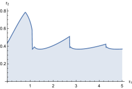
Figure 1: Extended stability region of Uçar system for $\alpha=1$

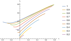
Figure 2: Critical curves of Uçar system for different values of $\alpha$

Now, we verify these stability results using numerical computations. In Fig. 3, we have taken $\tau_{1}=0.4$, $\tau_{2}=0.5$ and $\alpha=0.9$. These values are in stable region and the figure shows the orbit converging to an equilibrium state. In Fig. 4, we take the parameter values $\tau_{1}=1.6$, $\tau_{2}=1.4$ and $\alpha=0.9$ in unstable region. In this case, the system exhibit chaotic oscillations.

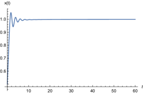
Figure 3: Stable orbit of Uçar system for $\alpha=0.9$, $\tau_{1}=0.4$ and $\tau_{2}=0.5$

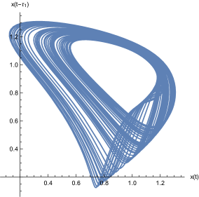
Figure 4: Chaotic attractor of Uçar system for $\alpha=0.9$, $\tau_{1}=1.6$ and $\tau_{2}=1.4$

Example 5.2

Consider the generalization of fractional order Ikeda equation [30] with two delays

$$D^{\alpha}x(t)=-3x\left(t-\tau_{1}\right)+24\sin\left(x\left(t-\tau_{2}\right)\right),\quad 0<\alpha\leq 1.$$ (23)

As discussed in [16], there are seven equilibrium points. The points $x_{0}=0$ and $x_{3,4}=\pm 7.49775$ are unstable whereas $x_{1,2}=\pm 2.7859$ and $x_{5,6}=\pm 7.95732$ are stable at $\tau_{1}=\tau_{2}=0$. The characteristic equation of the system (23) at the equilibrium point $x^{*}$ is

$$\lambda^{\alpha}=-3\exp(-\lambda\tau_{1})+24\cos(x^{*})\exp(-\lambda\tau_{2}).$$ (24)

If we take $x^{*}=x_{1,2}$ then the characteristic equation becomes

$$\lambda^{\alpha}=-3\exp(-\lambda\tau_{1})-22.4977\exp(-\lambda\tau_{2}).$$ (25)

This gives $a=-3$ and $b=-22.4977$. The critical curve in this case is given in Fig. 5 for $\alpha=0.7$.

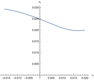
Figure 5: Critical curve of Ikeda system for $\alpha=0.7$

In Fig. 6, we have presented stable solution of system (23) with $\tau_{1}=0.02$ and $\tau_{2}=0.01$ in stable region. If we consider the values $\tau_{1}=0.01$ and $\tau_{2}=0.1$ in unstable region then we get chaotic attractor (cf. Fig. 7).

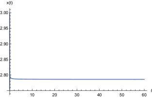
Figure 6: Stable orbit of Ikeda system for $\alpha=0.7$, $\tau_{1}=0.02$ and $\tau_{2}=0.01$

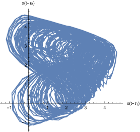
Figure 7: Chaotic attractor shown by Ikeda system for $\alpha=0.7$, $\tau_{1}=0.01$ and $\tau_{2}=0.1$

6 Conclusion

In [16], we have presented the complete analysis of the generalized equation involving delay. However, the analysis of the systems with multiple delay is not as simple as that of single delay. In this article, we have presented the expressions for critical values of generalized two delay system. We obtain the parametric relation between the delays $\tau_{1}$ and $\tau_{2}$. The region bounded by horizontal axis and the critical curve is stable region if the eigenvalues are stable at $\tau_{1}=\tau_{2}=0$. The nonlinear system may exhibit chaotic oscillations in unstable region. We also have presented numerical scheme to solve these systems. Further, the results are illustrated with two examples.

References

- [1] I. Podlubny, Fractional Differential Equations (Academic Press, New York, 1999).
- [2] S. G. Samko, A. A. Kilbas and O. I. Marichev, Fractional Integrals and Derivatives: Theory and Applications (Gordon and Breach, Yverdon, 1993).
- [3] A. A. Kilbas, H. M. Srivastava, J. J. Trujillo, Theory and applications of fractional differential equations (Elsevier, Amsterdam, 2006).
- [4] F. Mainardi, Fractional calculus and waves in linear viscoelasticity (Imperial College Press, London, 2010).
- [5] R. L. Magin, Fractional calculus in bioengineering (Begll House Publishers, USA, 2006).
- [6] X. Yang, D. Baleanu and H. M. Srivastava, Local Fractional Integral Transforms and Their Applications (Academic Press, London, 2015).
- [7] H. Smith, An introduction to delay differential equations with applications to the life sciences (Springer, New York, 2010).
- [8] M. Lakshmanan, D. V. Senthilkumar, Dynamics of nonlinear time-delay systems (Springer, Heidelberg, 2010).
- [9] C. Lainscsek, P. Rowat, L. Schettino, D. Lee, D. Song, C. Letellier, and H. Poizner, “Finger tapping movements of Parkinson’s disease patients automatically rated using nonlinear delay differential equations,” Chaos 22, 013119 (2012).
- [10] C. Lainscsek, and T. J. Sejnowski, “Electrocardiogram classification using delay differential equations,” Chaos 23, 023132 (2013)
- [11] D. Matignon, “Stability results for fractional differential equations with applications to control processing.” In: Computational Engineering in Systems and Application multiconference, vol. 2, pp. 963–968, IMACS, IEEE-SMC Proceedings, Lille, France, July (1996).
- [12] M. A. Pakzad and S. Pakzad, “Stability map of fractional order time-delay systems,” WSEAS Trans. Syst. 11(10), 541–550 (2012).
- [13] C. Bonnet and J. R. Partington, “Analysis of fractional delay systems of retarded and neutral type,” Automatica 38(7), 1133–1138 (2002).
- [14] C. Hwang, Y. C. Cheng, “A numerical algorithm for stability testing of fractional delay systems,” Automatica 42, 825–831 (2006).
- [15] S. Bhalekar, “Stability analysis of a class of fractional delay differential equations,” Pramana- Journal of Physics 81(2), 215–224 (2013).
- [16] S. Bhalekar, “Stability and bifurcation analysis of a generalized scalar delay differential equation,” Chaos 26(8), 084306 (2017).
- [17] S. Bhalekar and V. Daftardar-Gejji, “Fractional ordered Liu system with time-delay,” Commun. Nonlinear Sci. Numer. Simulat. 15(8), 2178–2191 (2010).
- [18] V. Daftardar-Gejji, S. Bhalekar and P. Gade, “Dynamics of fractional ordered Chen system with delay,” Pramana- Journal of Physics 79(1), 61–69 (2012).
- [19] S. Bhalekar, “Dynamical analysis of fractional order Ucar prototype delayed system,” Signals Image and Video Processing 6(3), 513–519 (2012).
- [20] S. Bhalekar, V. Daftardar-Gejji, D. Baleanu and R. Magin, “Fractional Bloch equation with delay,” Comput. Math. Appl. 61(5), 1355–1365 (2011).
- [21] S. Bhalekar, V. Daftardar-Gejji, D. Baleanu and R. Magin, “Generalized fractional order Bloch equation with extended delay,” Int. J. Bifurc. Chaos 22(4), 1250071 (2012).
- [22] J. K. Hale and W. Huang, “Global geometry of the stable regions for two delay differential equations,” J. Math. Anal. Appl. 178, 344–362 (1993).
- [23] J. Belair and S. A. Campbell, “Stability and bifurcations of equilibria in a multiple-delayed differential equation,” SIAM J. Appl. Math. 54, 1402–1424 (1994).
- [24] X. Li and S. Ruan, “Stability and bifurcation in delay differential equations with two delays,” J. Math. Anal. Appl. 236, 254–280 (1999).
- [25] X. P. Wu and L. Wang, “Zero-Hopf bifurcation analysis in delayed differential equations with two delays,” J. Franklin Inst. 354, 1484–1513 (2017).
- [26] P. Bi and S. Ruan, “Bifurcations in delay differential equations and applications to tumor and immune system interaction models,” SIAM J. Appl. Dyn. Sys. 12(4), 1847–1888 (2013).
- [27] S. Gakkhar and A. Singh, “Complex dynamics in a prey predator system with multiple delays,” Commun. Nonlinear Sci. Numer. Simulat. 17, 914–929 (2012).
- [28] V. Daftardar-Gejji, Y. Sukale and S. Bhalekar, “Solving fractional delay differential equations: A new approach,” Fract. Calc. Appl. Anal. 18, 400–418 (2015).
- [29] S. Bhalekar, “On the Uçar prototype model with incommensurate delays,” Signal, Image and Video Processing 8(4), 635–639 (2014).
- [30] J. G. Lu, “Chaotic dynamics of the fractional-order Ikeda delay system and its synchronization,” Chinese Physics 15(2) 301–305 (2006).