Reconstructing networks with unknown and heterogeneous errors

Abstract

The vast majority of network datasets contains errors and omissions, although this is rarely incorporated in traditional network analysis. Recently, an increasing effort has been made to fill this methodological gap by developing network reconstruction approaches based on Bayesian inference. These approaches, however, rely on assumptions of uniform error rates and on direct estimations of the existence of each edge via repeated measurements, something that is currently unavailable for the majority of network data. Here we develop a Bayesian reconstruction approach that lifts these limitations by not only allowing for heterogeneous errors, but also for single edge measurements without direct error estimates. Our approach works by coupling the inference approach with structured generative network models, which enable the correlations between edges to be used as reliable uncertainty estimates. Although our approach is general, we focus on the stochastic block model as the basic generative process, from which efficient nonparametric inference can be performed, and yields a principled method to infer hierarchical community structure from noisy data. We demonstrate the efficacy of our approach with a variety of empirical and artificial networks.

I Introduction

The study of network systems of various kinds constitutes a significant fraction of contemporary interdisciplinary research in physics, biology, computer science and social sciences, among other disciplines Barabási (2011). This is motivated in large part by the surging availability of network data during the past couple of decades, which describe the detailed interactions among constituents of large-scale complex systems, such as transportation networks, cell metabolism, social contacts, the internet, and various others. Despite the widespread growth of this field, its relative infancy is still noticeable in some aspects. In particular, even though sophisticated and successful models of network structure and function have been proposed, as well as powerful data analysis methods, most studies of empirical data are performed without taking into account measurement error. Most typically, real networks are represented as adjacency matrices, sometimes enriched with additional information such as edge weights and types, as well as various kinds of node properties, the validity of which is simply taken for granted. But as is true for any empirical scenario, network data is subject to observational errors: parts of the network might not have been recorded, and the parts that have might be wrong. Although this problem has been recognized in the past in several studies Marsden (1990); Butts (2003); Liben-Nowell and Kleinberg (2007); Clauset et al. (2008); Guimerà and Sales-Pardo (2009); Lü and Zhou (2011); Žnidaršič et al. (2012); Squartini and Garlaschelli (2017); Newman (2018a, b), the practice of ignoring measurement error is still mainstream, and robust methods to take it into account are underdeveloped. This is in no small part due to the fact that most available network data contain no quantitative error assessment information of any kind, thus preventing primary experimental uncertainties to be propagated up the chain of analysis.

In this work we formulate a principled method to reconstruct networks that have been imperfectly measured. We do so by simultaneously formulating generative models of network structure — that incorporate degree heterogeneity, modules and hierarchies — as well as models of the noisy measurement process. By performing Bayesian statistical inference of this joint model, we are able to reconstruct the underlying network given an imperfect measurement affected by observational noise. Importantly, our method works also when a single measurement of the underlying network has been made, and the noise magnitudes are unknown. This means it can be directly applied to the majority of network data without available error estimates. In addition to this, our method is capable of extracting hierarchical modular structure from such noisy networks, thus generalizing the task of community detection to this uncertain setting.

Our method is equally applicable when information on measurement error is available, either as repeated measurements or as estimated edge probabilities. For this class of data, we construct a general model that allows for heterogeneous errors, that vary in different parts of the network. We show strong empirical evidence for the existence of this kind of heterogeneity, and demonstrate the efficacy of our method to include it in the reconstruction.

Our method shares some underlying similarities with well known model-based approaches of edge prediction Clauset et al. (2008); Guimerà and Sales-Pardo (2009), but is different from them in fundamental aspects. Most importantly, model-based edge prediction methods yield relative probabilities of edges existing or not, given a generative model fitted to the observed data. These relative probabilities can be used to reconstruct a network provided one knows how many edges are missing or spurious. Our method obviates the need for this information (which is in general unknown), and yields not only a reconstructed network, but also the uncertainty estimate that must come with it, via a posterior distribution over all possible reconstructions. Thus our method realizes the underlying promise of reconstruction that motivates most edge prediction methods, but in a principled and nonparametric way.

We form the basis of our reconstruction scenario on Ref. Newman (2018a), which defined a statistical inference method based on multiple measurements of network data, but here we use a different approach based on nonparametric Bayesian inference, combined with community detection. This yields a more powerful method that, differently from Ref. Newman (2018a), can be applied also when the network data does not contains any kind of primary error estimate, such as when the edges and nonedges have been measured only once.

This work is organized as follows. In Sec. II we formulate our Bayesian reconstruction framework. In Sec. II.1 we present our measurement model, and in Sec. II.2 we illustrate the use of our reconstruction method with some examples. In Sec. II.3 we perform a detailed analysis of the reconstruction performance of the method, as well as its use to provide estimates of various network properties. In Sec. II.4 we employ our approach to some empirical network data without primary error estimates, and evaluate their reliability. In Sec. II.5 we extend our method to heterogeneous errors, and use it to analyze network data with multiple measurements. In Sec. III we show how our method can be extended to situations where the arbitrary error estimates are extrinsically provided, and we finalize in Sec. IV with a conclusion.

II Bayesian network reconstruction

The scenario we consider is one where instead of a direct observation of a network $\bm{A}$, we perform a noisy measurement $\bm{\mathcal{D}}$ that contains only indirect information about $\bm{A}$. The task of network reconstruction is then to obtain $\bm{A}$ from $\bm{\mathcal{D}}$. The approach we take is to perform statistical inference, where first we model the network generating process via a probability

$$P(\bm{A}|\theta),$$ (1)

where $\theta$ are arbitrary model parameters. The entire data generating process is then completed by modelling also the noisy measurement,

$$P(\bm{\mathcal{D}}|\bm{A},\phi),$$ (2)

conditioned on the generated network $\bm{A}$ (the “true” network) and some further parameters $\phi$. Given this general setup, the reconstruction procedure consists of determining $\bm{A}$ from the posterior distribution

$$P(\bm{A}|\bm{\mathcal{D}})=\frac{P(\bm{\mathcal{D}}|\bm{A})P(\bm{A})}{P(\bm{\mathcal{D}})},$$ (3)

where

$$P(\bm{\mathcal{D}}|\bm{A})=\int P(\bm{\mathcal{D}}|\bm{A},\phi)P(\phi)\;\mathrm{d}\phi,$$ (4)

is the marginal probability of the measurements $\bm{\mathcal{D}}$, and

$$P(\bm{A})=\int P(\bm{A}|\theta)P(\theta)\;\mathrm{d}\theta,$$ (5)

is the prior probability for $\bm{A}$, summed over all possible parameter choices, weighted according to their (hyper-)prior probabilities. The remaining term $P(\bm{\mathcal{D}})=\sum_{\bm{A}}P(\bm{\mathcal{D}}|\bm{A})P(\bm{A})$ is a normalization constant that corresponds to the total probability — or evidence — for the observed measurement. In the above, the probabilities $P(\theta)$ and $P(\phi)$ encode our prior knowledge (or lack thereof) about the network generation and measurement processes, respectively. With these at hand, Eq. 3 assigns the probability of a given network $\bm{A}$ being responsible for measurement $\bm{\mathcal{D}}$. Importantly, this distribution defines an ensemble of possibilities for the underlying network $\bm{A}$ that incorporates the amount uncertainty resulting from the measurement. This contrasts with reconstruction approaches that attempt to reproduce a single network, although within the above framework we could also attempt to find the single most likely reconstruction that maximizes Eq. 3, i.e. a maximum posterior point estimate. However, as we will see below, this is not the most appropriate point estimate, as it tends to incorporate noise from the data, biasing the reconstruction. Instead, we should consider the consensus of the full posterior distribution, which can also give us an estimation of uncertainty.

The above framework is general, and can be used for any kind of generative and measurement processes. Here, we are interested in those that can be used to describe the large-scale modular structures of networks, characterized by the partition of the nodes into groups $\bm{b}=\{b_{i}\}$, where $b_{i}\in\{1,\dots,B\}$ is group membership of node $i$. The simplest and most commonly used model for this is the stochastic block model (SBM) Holland et al. (1983),

$$P(\bm{A}|\bm{\omega},\bm{b})=\prod_{i<j}\omega_{b_{i},b_{j}}^{A_{ij}}(1-\omega_{b_{i},b_{j}})^{1-A_{ij}}$$ (6)

where $\omega_{rs}$ is the probability of an edge existing between nodes of groups $r$ and $s$. Alternatively, we could also consider a more realistic version called the degree-corrected SBM (DC-SBM) Karrer and Newman (2011),

$$P(\bm{A}|\bm{\lambda},\bm{\kappa},\bm{b})=\prod_{i<j}\frac{e^{-\kappa_{i}\kappa_{j}\lambda_{b_{i},b_{j}}}(\kappa_{i}\kappa_{j}\lambda_{b_{i},b_{j}})^{A_{ij}}}{A_{ij}!},$$ (7)

where $\lambda_{rs}$ controls the number of edges between groups $r$ and $s$ and $\kappa_{i}$ the expected degree of node $i$. This model variant decouples the degrees from the group memberships, allowing for arbitrary degree variability inside modules, a feature often found to be more compatible with real networks Peixoto (2017). (Note that the DC-SBM generates multigraphs with $A_{ij}\in\mathbb{N}$, whereas the SBM above generates simple graphs with $A_{ij}\in\{0,1\}$, as our framework requires. In appendix D we amend this inconsistency.) Using the above, we compute the marginal network probability as

$$P(\bm{A})=\sum_{b}P(\bm{A}|\bm{b})P(\bm{b}),$$ (8)

with

$$P(\bm{A}|\bm{b})=\int P(\bm{A}|\bm{\lambda},\bm{\kappa},\bm{b})P(\bm{\kappa}|\bm{b})P(\bm{\lambda}|\bm{b})\;\mathrm{d}\kappa\,\mathrm{d}\lambda,$$ (9)

integrated over the remaining model parameters, weighted by their respective prior probabilities. However, although Eq. 9 can be computed exactly Peixoto (2017), the complete marginal of Eq. 8 cannot, as it involves an intractable sum over all possible network partitions. Hence, instead of computing directly the posterior of Eq. 3, we obtain the joint posterior

$$P(\bm{A},\bm{b}|\bm{\mathcal{D}})=\frac{P(\bm{\mathcal{D}}|\bm{A})P(\bm{A}|\bm{b})P(\bm{b})}{P(\bm{\mathcal{D}})},$$ (10)

which involves only quantities that can be computed exactly, except $P(\bm{\mathcal{D}})$, which as we will shortly see, is unnecessary for the inference procedure. We do the above without any loss, as the original posterior of Eq. 3 can be obtained by marginalization, i.e.

$$P(\bm{A}|\bm{\mathcal{D}})=\sum_{\bm{b}}P(\bm{A},\bm{b}|\bm{\mathcal{D}}).$$ (11)

This means that if we can sample from the joint posterior $P(\bm{A},\bm{b}|\bm{\mathcal{D}})$, we can compute any estimate $\hat{y}$ of a network property $y(\bm{A})$ (e.g. the clustering coefficient) over the full marginal $P(\bm{A}|\bm{\mathcal{D}})$ by averaging it over the joint posterior, i.e.

$$\hat{y}=\sum_{\bm{A}}y(\bm{A})P(\bm{A}|\bm{\mathcal{D}})=\sum_{\bm{A},\bm{b}}y(\bm{A})P(\bm{A},\bm{b}|\bm{\mathcal{D}}).$$ (12)

The procedure we use to sample from the posterior distribution is Markov chain Monte Carlo (MCMC). We consider move proposals of the kind $P(\bm{b}^{\prime}|\bm{A},\bm{b})$ and $P(\bm{A}^{\prime}|\bm{A},\bm{b})$ for the partition and network, respectively, and accept the proposal according to the Metropolis-Hastings Metropolis et al. (1953); Hastings (1970) probability

$$\min\left(1,\frac{P(\bm{A}^{\prime},\bm{b}^{\prime}|\bm{\mathcal{D}})P(\bm{A}|\bm{A}^{\prime},\bm{b}^{\prime})P(\bm{b}|\bm{A}^{\prime},\bm{b}^{\prime})}{P(\bm{A},\bm{b}|\bm{\mathcal{D}})P(\bm{A}^{\prime}|\bm{A},\bm{b})P(\bm{b}^{\prime}|\bm{A},\bm{b})}\right),$$ (13)

which enforces detailed balance. If the move proposals are ergodic, i.e. they allow every network $\bm{A}$ and partition $\bm{b}$ to be proposed eventually, this algorithm will generate samples from the posterior distribution $P(\bm{A},\bm{b}|\bm{\mathcal{D}})$ after a sufficiently large number of iterations (usually determined by requiring that statistical properties of the chain, such as average log-probability, become stationary). The ratio in Eq. 13 can be determined exactly without computing the intractable constant $P(\bm{\mathcal{D}})$ in Eq. 10, making this method asymptotically exact. We give more technical details of our MCMC procedure in Appendix B.

The above setup is still sufficiently general that it can be used with any variant of the SBM. In particular, here we will make extensive use of the hierarchical DC-SBM (HDC-SBM) Peixoto (2014a, 2017), which differs from the DC-SBM in that a nested hierarchy of priors and hyperpriors is used in place of the single prior $P(\bm{\lambda}|\bm{b})$ for the connections between groups. In this model, groups are clustered hierarchically into meta-groups, yielding a nested hierarchical partition $\{\bm{b}^{l}\}$, where $\bm{b}^{l}$ is the partition of the groups in level $l$. As discussed in Refs. Peixoto (2014a, 2017), this choice of structured priors removes a tendency of noninformative priors to underfit Peixoto (2013), and enables the detection of structures at multiple scales, while at the same time remaining unbiased with respect to different types of mixing patterns. Its posterior distribution is obtained in the same fashion, following the framework above, simply by replacing $\bm{b}\to\{\bm{b}^{l}\}$.

In the following, whenever we mention that we sample from the posterior $P(\bm{A}|\bm{\mathcal{D}})$, it is meant we sample from the joint posterior $P(\bm{A},\bm{b}|\bm{\mathcal{D}})$, and marginalize over $\bm{b}$, as described above. The same is true when using the hierarchical model, i.e. we sample from $P(\bm{A},\{\bm{b}^{l}\}|\bm{\mathcal{D}})$, and marginalize over the hierarchical partitions $\{\bm{b}^{l}\}$.

The main difference from typical community detection based on statistical inference is that here we are not only interested in detecting modules in networks, but also inferring the network itself. Therefore, both the network and its partition into (hierarchical) groups are inferred from indirect data. As we will see, the simultaneous detection of modules offers a substantial advantage to the reconstruction task, as it allows correlations among edges to inform it. This means that we are able to perform reconstruction in situations which would otherwise be impossible. But before we proceed, we need to model the measurement process itself, as we do in the following.

II.1 Noisy network measurements

Here we will consider the scenario used in Ref. Newman (2018a), where the edges of a network are measured directly and repeatedly, but the process is noisy, and potentially distorts the network. In particular, we will assume that for each node pair $(i,j)$ we perform $n_{ij}$ distinct measurements, and record $x_{ij}$ positive outcomes, i.e. an edge is observed. For each observation, we have a probability $p$ of observing a missing edge (i.e. a false negative) and a probability $q$ of observing a spurious edge (i.e. a false positive), depending in each case if the underlying network possesses or not an edge $(i,j)$. Thus, for each edge the observation probability is distributed according to a binomial distribution, with a success rate that depends on whether an edge exists in the underlying network, i.e.

$$P(x_{ij}|n_{ij},A_{ij},p,q)=\\ {n_{ij}\choose x_{ij}}\left[(1-p)^{x_{ij}}p^{n_{ij}-x_{ij}}\right]^{A_{ij}}\left[q^{x_{ij}}(1-q)^{n_{ij}-x_{ij}}\right]^{1-A_{ij}}.$$ (14)

Thus, the joint likelihood for the whole set of measurements $\bm{x}=\{x_{ij}\}$ is

$$P(\bm{x}|\bm{n},\bm{A},p,q)=\prod_{i<j}P(x_{ij}|n_{ij},A_{ij},p,q)\\ =\left[\prod_{i<j}{n_{ij}\choose x_{ij}}\right](1-p)^{\mathcal{T}}p^{\mathcal{E}-\mathcal{T}}q^{\mathcal{X}-\mathcal{T}}(1-q)^{\mathcal{M}-\mathcal{X}-\mathcal{E}+\mathcal{T}},$$ (15)

written in terms of the following summary quantities,

$$\mathcal{M} =\sum_{i<j}n_{ij}, \mathcal{X} =\sum_{i<j}x_{ij},$$ (16)

$$\mathcal{E} =\sum_{i<j}n_{ij}A_{ij}, \mathcal{T} =\sum_{i<j}x_{ij}A_{ij},$$ (17)

where $\mathcal{M}$ is the total number of measurements (edge or nonedge), $\mathcal{X}$ is the total number of observed edges, $\mathcal{E}$ is the total number of measured edges and $\mathcal{T}$ is the total number of correctly observed edges. From this, we also identify the total number of false positives (spurious edges) as $\mathcal{X}-\mathcal{T}$ and of false negatives (missing edges) as $\mathcal{E}-\mathcal{T}$.

To proceed with our calculation we need to specify the degree of prior knowledge we have on the error rates $p$ and $q$. We can express this most naturally with a Beta distribution,

$$P(p|\alpha,\beta)=\frac{p^{\alpha-1}(1-p)^{\beta-1}}{\mathcal{B}(\alpha,\beta)}$$ (18)

where $\mathcal{B}(x,y)=\Gamma(x)\Gamma(y)/\Gamma(x+y)$ is the Euler beta function, and $\Gamma(x)$ is the gamma function, and likewise for $P(q|\mu,\nu)$, with hyperparameters $\mu$ and $\nu$. As illustrated in Fig. 17 of appendix A, a value of $\alpha=\beta=1$ encodes a maximum amount of prior ignorance with respect to $p$, which is then uniformly distributed in the unit interval. Conversely, values $\alpha\to\infty$ and $\beta\to\infty$ converge to a Dirac delta function centered at $\alpha/(\alpha+\beta)$, amounting to a maximum certainty for a particular value of $p$, and therefore intermediary values of $\alpha$ and $\beta$ interpolate between these two extremes (and analogously for $q$ with $\mu$ and $\nu$). With this, we can compute the integrated likelihood

$$P(\bm{x}|\bm{n},\bm{A},\alpha,\beta,\mu,\nu)\\ =\int P(\bm{x}|\bm{n},\bm{A},p,q)P(p|\alpha,\beta)P(q|\mu,\nu)\;\mathrm{d}p\,\mathrm{d}q\\ =\left[\prod_{i<j}{n_{ij}\choose x_{ij}}\right]\frac{\mathcal{B}(\mathcal{E}-\mathcal{T}+\alpha,\mathcal{T}+\beta)}{\mathcal{}B(\alpha,\beta)}\times\\ \frac{\mathcal{B}(\mathcal{X}-\mathcal{T}+\mu,\mathcal{M}-\mathcal{X}-\mathcal{E}+\mathcal{T}+\nu)}{\mathcal{B}(\mu,\nu)}.$$ (19)

The noninformative case $\alpha=\beta=\mu=\nu=1$ simplifies further to

$$P(\bm{x}|\bm{n},\bm{A})=\left[\prod_{i<j}{n_{ij}\choose x_{ij}}\right]\times\\ {\mathcal{E}\choose\mathcal{T}}^{-1}\frac{1}{\mathcal{E}+1}{\mathcal{M}-\mathcal{E}\choose\mathcal{X}-\mathcal{T}}^{-1}\frac{1}{\mathcal{M}-\mathcal{E}+1}.$$ (20)

The above noninformative generative process can also be equivalently interpreted as first choosing the number of false positives $\mathcal{X}-\mathcal{T}$ uniformly from the interval $[0,\mathcal{M}-\mathcal{E}]$ and then selecting them uniformly at random from the possible set with ${\mathcal{M}-\mathcal{E}\choose\mathcal{X}-\mathcal{T}}$ elements, and similarly choosing the number of false-negatives $\mathcal{E}-\mathcal{T}$ uniformly in the interval $[0,\mathcal{E}]$ and the false-negatives from the set of size ${\mathcal{E}\choose\mathcal{E}-\mathcal{T}}={\mathcal{E}\choose\mathcal{T}}$.

With the integrated likelihood in place, we can finally complete the posterior distribution of Eq. 3 with $\bm{\mathcal{D}}=(\bm{n},\bm{x})$, which in this case becomes,

$$P(\bm{A}|\bm{n},\bm{x},\alpha,\beta,\mu,\nu)=\frac{P(\bm{x}|\bm{n},\bm{A},\alpha,\beta,\mu,\nu)P(\bm{A})}{P(\bm{x}|\alpha,\beta,\mu,\nu)}.$$ (21)

For $P(\bm{A})$ we will use the SBM and sample $\bm{A}$ using MCMC from the joint posterior $P(\bm{A},\bm{b}|\bm{n},\bm{x},\alpha,\beta,\mu,\nu)$, as discussed previously.

Even though we have integrated over the error probabilities $p$ and $q$ in the above, we can nevertheless obtain their posterior estimates by averaging from the above posterior

$$P(p|\bm{n},\bm{x},\alpha,\beta,\mu,\nu)=\\ \sum_{\bm{A}}P(p|\bm{n},\bm{x},\bm{A},\alpha,\beta)P(\bm{A}|\bm{n},\bm{x},\alpha,\beta,\mu,\nu),$$ (22)

using the posterior for $p$ conditioned on the network $\bm{A}$,

$$P(p|\bm{n},\bm{x},\bm{A},\alpha,\beta)=\frac{p^{\mathcal{E}-\mathcal{T}+\alpha-1}(1-p)^{\mathcal{T}+\beta-1}}{\mathcal{B}(\mathcal{E}-\mathcal{T}+\alpha,\mathcal{T}+\beta)}$$ (23)

and likewise for $q$ with

$$P(q|\bm{n},\bm{x},\bm{A},\mu,\nu)=\frac{q^{\mathcal{X}-\mathcal{T}+\mu-1}(1-q)^{\mathcal{M}-\mathcal{X}-\mathcal{E}+\mathcal{T}+\mu-1}}{\mathcal{B}(\mathcal{X}-\mathcal{T}+\mu,\mathcal{M}-\mathcal{X}-\mathcal{E}+\mathcal{T}+\nu)}.$$ (24)

In the following, we will most often assume the noninformative case $\alpha=\beta=\nu=\mu=1$, corresponding to the maximum lack of prior knowledge about the measurement noise. In order to unclutter our expressions, if this is the case we will simply omit those hyperparameters from the posterior distribution, i.e. $P(\bm{A}|\bm{n},\bm{x})\equiv P(\bm{A}|\bm{n},\bm{x},\alpha=1,\beta=1,\mu=1,\nu=1)$.

II.1.1 Single edge measurements

As we increase the number of measurements $n_{ij}$ of each pair of nodes, we should expect also to increase the accuracy of the reconstruction, resulting in a posterior distribution $P(\bm{A}|\bm{n},\bm{x})$ that is very sharply peaked around the true underlying network. Although this scenario is plausible, and indeed desirable under controlled experimental conditions, this is not representative of the majority of the network data that are currently available. In fact, inspecting comprehensive network catalogs such as KONECT Kunegis (2013) and ICON Clauset et al. (2016) reveals a very pauper set of network data that can be cast under this setting of repeated measurements. On the contrary, the vast majority of them offer only a single adjacency matrix without quantitative error estimates of any kind. Needless to say, this is no reason to assume that they do not, in fact, contain errors, only that they have not been assessed or published.

Here we propose an approach of assessing the uncertainty of this dominating kind of network data by interpreting it as a single measurement with unknown errors rates, using the framework outlined above. In more detail, we assume that $n_{ij}=1$ for every pair $i,j$ and that the single measurements $x_{ij}\in\{0,1\}$, correspond to the reported adjacency matrix. The lack of knowledge about the underlying error rates $p$ and $q$ can be expressed by choosing $\alpha=\beta=\mu=\nu=1$, in which case it is assumed that they both lie a priori anywhere in the unit interval. At first we may wonder if this approach has any chance of succeeding, since the lack of knowledge about the error rates means that the network could have been modified in arbitrary ways, such that the true underlying network is radically different from what has been observed. Indeed, if we define the distance between measured and generated networks,

$$d(\bm{A},\bm{x})=\sum_{i<j}\left|A_{ij}-x_{ij}\right|=(\mathcal{E}-\mathcal{T})+(\mathcal{X}-\mathcal{T}),$$ (25)

which equals the sum of false negatives and false positives, we have that according to Eq. 20, the expected distance over many measurements is

$$\bar{d}(\bm{A})=\sum_{\bm{x}}d(\bm{A},\bm{x})P(\bm{x}|\bm{n},\bm{A})={N\choose 2}/2,$$ (26)

which is half the maximum possible distance of ${N\choose 2}$, which might lead us to conclude that our noise model will invariably destroy the network beyond the possibility of reconstruction, regardless of its original structure. What changes this picture is the fact that the posterior distribution $P(\bm{A}|\bm{x},\bm{n})$ of Eq. 21 will in fact be more concentrated on the generated network than the implied by the above, and ultimately will depend crucially on our generative process $P(\bm{A})$. The first point can be made by assuming a fully random generative model,

$$P(\bm{A}|\omega)=\prod_{i<j}\omega^{A_{ij}}(1-\omega)^{1-A_{ij}},$$ (27)

which means that the true networks being measured are assumed to be completely random, given a particular density $\omega$. The full prior can be obtained by a noninformative assumption $P(\omega)=1$, which yields

$$P(\bm{A}) =\int P(\bm{A}|\omega)P(\omega)\,\mathrm{d}\omega,$$ (28)

$$={{N\choose 2}\choose E}^{-1}\frac{1}{{N\choose 2}+1},$$ (29)

with $E=\sum_{i<j}A_{ij}=\mathcal{E}$ being the total number of edges, which is equivalent to sampling to the total number of edges from the interval $[0,{N\choose 2}]$ and then a fully random graph with that number of edges. Combining this with Eq. 20, yields the posterior distribution, which can be written as the product of two conditional probabilities,

$$P(\bm{A}|\bm{x},\bm{n})=P(\bm{A}|\bm{x},\mathcal{T},\mathcal{E})P(\mathcal{T},\mathcal{E}|\bm{x}),$$ (30)

with

$$P(\bm{A}|\bm{x},\mathcal{T},\mathcal{E})={\mathcal{X}\choose\mathcal{X}-\mathcal{T}}^{-1}{{N\choose 2}-X\choose\mathcal{E}-\mathcal{T}}^{-1}$$ (31)

corresponding to the uniform sampling of $\bm{A}$ with exactly $\mathcal{E}-\mathcal{T}$ false negatives and $\mathcal{X}-\mathcal{T}$ false positives, and

$$P(\mathcal{T},\mathcal{E}|\bm{x})\propto\frac{[\mathcal{T}\leq\mathcal{E}][\mathcal{T}\leq\mathcal{X}]}{(\mathcal{E}+1)[{N\choose 2}-\mathcal{E}+1]}$$ (32)

with $[\cdots]$ being the Inverson bracket that equals $1$ if the condition inside it is true, or $0$ otherwise, determines the posterior probability of the number of false negatives and false positives, up to a normalization constant. Although this distribution decays for values of $\mathcal{E}$ larger than $0$, the decay is slow with $\sim 1/\mathcal{E}$, and hence, on average, the inferred networks $\bm{A}$ sampled from $P(\bm{A}|\bm{x},\bm{n})$ will be dense, yielding large distances $d(\bm{A},\bm{A}^{*})$ if the true generated network $\bm{A}^{*}$ is sparse. Although the posterior distribution of false negatives and positives resulting from $P(\mathcal{T},\mathcal{E}|\bm{x})$ is not uniformly distributed in the allowed interval, it is also not sufficiently concentrated to enable any reasonable accuracy in the reconstruction, regardless of how large the network is. What changes this considerably is to replace the fully random model of Eq. 28 by a more structured model. The key observation here is that the modifications induced by the error rates $p$ and $q$ affect uniformly every edge and nonedge, and thus with structured models we can exploit the observed correlations in the measurements $\bm{x}$ to infer the underlying network $\bm{A}$, and in fact even the error rates $p$ and $q$, which are a priori unknown.

Figure 1: (a) Illustration of a hypothetical measured network, with a priori unknown errors, but from which error estimates can be made: the lack of edges between groups 2 and 3, 3 and 4, 2 and 4, and 1 and 3 implies that the probability $q$ of missing edges is likely to be low. Similarly, the large internal density of group 3 (which forms a clique of 10 nodes) implies that the missing edge probability $p$ must be low as well. (b) How the network in (a) would look like for higher values of $p$ and $q$. (c) The distribution of marginal edge probabilities $p_{ij}$ between every node pair, for a fit of the HDC-SBM on the openflights data (see Appendix E), measured with different values of the noise parameters $(p,q)$. As the noise magnitudes increase, the probabilities become less heterogeneous, and concentrate in narrower intervals. Hence, the inference of broad connection probabilities from data rules out the existence of strong noise in the measurement.

We illustrate this by considering the non-degree-corrected SBM, where networks are generated with probability

$$P(\bm{A}|\bm{\omega},\bm{b})=\prod_{i<j}\omega_{b_{i}b_{j}}^{A_{ij}}(1-\omega_{b_{i}b_{j}})^{1-A_{ij}}.$$ (33)

The final likelihood for the measurements $\bm{x}$ in this case will be identical to an effective SBM, given by

$$P(\bm{x}|\bm{n},p,q,\bm{\omega},\bm{b}) =\sum_{\bm{A}}P(\bm{x}|\bm{n},\bm{A},p,q)P(\bm{A}|\bm{\omega},\bm{b})$$ (34)

$$=\prod_{i<j}{\omega_{b_{i}b_{j}}^{\prime}}^{x_{ij}}(1-\omega_{b_{i}b_{j}}^{\prime})^{1-x_{ij}}$$ (35)

where

$$\omega_{rs}^{\prime}=(1-p-q)\omega_{rs}+q$$ (36)

are the new effective SBM probabilities that have been scaled and shifted by the measurement noise. Suppose, for simplicity, that we know the true network partition $\bm{b}$, and that the number of groups is very small compared to the number of nodes in each group. In this situation, the posterior distribution for $\bm{\omega}^{\prime}$ should be tightly peaked around the maximum likelihood estimate $\bm{\hat{\omega}^{\prime}}$,

$$\hat{\omega}^{\prime}_{rs}=(1-p-q)\omega_{rs}+q=\frac{e_{rs}}{n_{r}n_{s}},$$ (37)

where $e_{rs}=\sum_{ij}x_{ij}\delta_{b_{i},r}\delta_{b_{j},s}$ is the number of observed edges between groups $r$ and $s$ (or twice that for $r=s$) and $n_{r}$ is the number of nodes in group $r$. The joint posterior distribution for $p$ and $q$ will then be asymptotically given by

$$P(p,q|\bm{x},\bm{n},\bm{b})\propto\int P(\bm{x}|\bm{n},p,q,\bm{\omega},\bm{b})P(\bm{\omega}|\bm{b})\;\mathrm{d}\bm{\omega}\\ \begin{aligned} &\propto\prod_{r\leq s}\int_{0}^{1}\delta((1-p-q)\omega_{rs}+q-e_{rs}/n_{r}n_{s})P(\omega_{rs}|\bm{b})\;\mathrm{d}\omega_{rs}\\ &\propto\prod_{r\leq s}\left[0\leq\frac{e_{rs}/n_{r}n_{s}-q}{1-p-q}\leq 1\right]\frac{P\left(\frac{e_{rs}/n_{r}n_{s}-q}{1-p-q}\middle|\bm{b}\right)}{1-p-q},\end{aligned}$$ (38)

up to normalization, where $[\cdots]$ is again the Inverson bracket. The constraints above imply that the inferred error rates will be bounded by the maximum and minimum inferred connection probabilities, i.e.

$$\hat{q} \leq\min_{rs}\frac{e_{rs}}{n_{r}n_{s}},$$ (39)

$$\hat{p} \leq 1-\max_{rs}\frac{e_{rs}}{n_{r}n_{s}}.$$ (40)

These bounds mean that if we have not observed many edges between groups $r$ and $s$, this implies that $q$ could not have been very large. If instead we do observe many edges between these groups, then this means that the value of $p$ could not have been very large either (see Fig. 1a and b). This holds for every pair of groups $r$ and $s$, but the values of $p$ and $q$ are global. Therefore, as long as the inferred SBM probabilities are sufficiently heterogeneous, they should constrain the inferred error rates to narrow intervals — which will also constrain the inferred number of false negatives and false positives (see Fig. 1c). On the other hand, if the model probabilities are homogeneous, the posterior distribution for the errors will be broad, and the quality of the reconstruction will be poor. Therefore, the success of this approach depends ultimately on the observed networks being sufficiently structured, and of our models being capable of describing them.

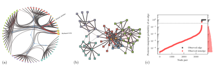
Figure 2: Network of social associations between 9/11 terrorists Krebs (2002a, b). This network was measured by potentially unreliable means, but no quantitative error estimates are known, and no repeated measurements were made. In (a) and (b) is shown the inferred network according to our method — which does not require direct error estimates or repeated measurements — where the edge thickness indicates the posterior marginal probability of an edge existing. In (a) the inferred hierarchical structure is shown, with pie charts on the nodes indicating the marginal probabilities of group memberships, and in (b) a spatial layout of the same network shows the lowest level of the hierarchy as the node colors. The edge shown in red is inferred as existing with a large probability, despite not being measured. Other potentially missing edges are also shown in red, with a probability given by their thickness and opacity. In (c) is shown the marginal probability of edge existence for all node pairs, indicating a fair amount of inferred reliability — with the exception of the single missing edge highlighted in (a) and (b) — despite the lack of direct error estimates in the data. The horizontal line marks a 1/3 probability as a visual aid. The missing edge corresponds to a connection between Mohamed Atta and Waleed Alshehri, which was not considered in Refs. Krebs (2002a, b), but is corroborated by reports that they shared an apartment in Berlin, and met previously in Spain.

The above means that we have a better chance of accurate reconstruction if our models are capable of detecting heterogeneous connection probabilities among nodes. A fully uniform model like the Erdős-Renyi of Eq. 28 (equivalent to a SBM with only one group) will exhibit the worse possible performance. The DC-SBM, on the other hand, should in general perform better than the SBM, since it is capable of capturing degree heterogeneity inside groups, which is a common feature of many networks Karrer and Newman (2011); Peixoto (2017). The HDC-SBM Peixoto (2014a, 2017) should perform even better, since its tendency not to underfit means it can detect statistically significant structures at smaller scales.

Finally, it must also be noted that when performing only single measurements, there remains an unavoidable identification problem, where it becomes impossible to fully distinguish a network that has been sampled from a SBM with parameters $\bm{\omega}$ and error rates $p$ and $q$ from the same network sampled from a SBM with parameters $\bm{\omega}^{\prime}$ given by Eq. 36 and error rates $p=q=0$ (and in fact any interpolation between these two extremes). This uncertainty, however, will be reflected in the variance of the posterior distribution, and serves as a worse-case estimation of the error rates, which ultimately can be improved either by incorporating better prior knowledge (e.g. via the hyperparameters $\alpha,\beta,\nu$ and $\mu$) or performing multiple measurements.

II.2 Empirical examples

Before we proceed further with a systematic analysis of our reconstruction method, we illustrate its behavior with some empirical data that are likely to contain errors and omissions. We begin with the network of social associations between 62 terrorists responsible for the 9/11 attacks Krebs (2002a, b). The existence of an edge between two terrorists is established if there is evidence they interacted directly in some way, e.g. if they attended the same college or shared an address. Clearly, this approach is inherently unreliable, as investigators may either fail to record evidence, or the evidence recorded may be simply erroneous. Nevertheless, although this potential unreliability was acknowledged in Refs. Krebs (2002a, b), is was not assessed quantitatively, and the data presented there is a single adjacency matrix with no error estimates. Therefore it serves as a suitable candidate for the application of our reconstruction method. When applied to this dataset, our approach yields the results seen in Fig. 2, which shows the marginal posterior probability of each possible edge in the network, in addition to the hierarchical modular structured captured by the HDC-SBM. Our method identifies the organization into a few largely disconnected cells, typical of terrorist groups. When ranking the potential edges according to their marginal posterior probability, as shown in Fig. 2c, we have that all observed edges are more likely to be true edges than any of the nonedges, indicating a fair degree of inferred reliability. The observed nonedges have a probability substantially smaller than the observed edges of being edges, with the sole exception of a connection between Mohamed Atta (one of the main leaders) and Waleed al-Shehri, which was not considered in Refs. Krebs (2002a, b), but to which our method ascribes a reasonably high probability of $0.48$. Atta is connected to all members of al-Shehri’s group, and according to the HDC-SBM the sole missing link between them is therefore suspicious. Indeed, journalistic reports place both individuals occasionally sharing an apartment in Berlin, and meeting at least once in Spain, prior to the attacks, which seems to corroborate our reconstruction. The remaining observed nonedges have a probability of $0.15$ or smaller, which should not be outright discarded, and could serve as candidates for further investigation.

We now move to another social network, namely the interactions between 34 members of a karate club, originally studied by Zachary Zachary (1977). This network has been widely used to evaluate community detection methods, after its use for this purpose in Ref. Girvan and Newman (2002). It was recorded just before the split of the club in two disjoint groups after a conflict, and many community detection methods are capable of accurately predicting the split by detecting communities from this snapshot. However, not only does the original publication of Ref. Zachary (1977) omits any assessment of measurement uncertainties, but also it clearly contains one obvious error: the adjacency matrix $\bm{A}$ published in the original study, although it is supposed to be symmetric, contains two inconsistent entries with $A_{ij}\neq A_{ji}$, for $(i,j)=(23,34)$, creating an ambiguity about the existence of this particular edge. The authors of Ref. Girvan and Newman (2002) made the decision of assuming $A_{23,34}=1$, even though there seems to be no obvious reason to decide either way a priori. The vast majority of other works in the area followed suit (possibly inadvertently), thus incorporating this potential, though arguably small, error in their analysis. Here we tackle this reconstruction problem by mapping the uncertain dataset of Ref. Zachary (1977) to our framework. Since each node pair $(i,j)$ was also presented reversed $(j,i)$, we consider these as independent measurements, such that $n_{ij}=2$ for every pair $(i,j)$. Since the measurements were consistent for all but one pair, we have $x_{ij}=2$ or $0$, except for the offending entry with $x_{(23,34)}=1$. Based on this we employed our reconstruction approach to obtain $P(\bm{A}|\bm{n},\bm{x})$, using as generative processes the Erdős-Rényi (ER) model (equivalent to a SBM with only one group, $B=1$), the configuration model (CM) (equivalent to a DC-SBM with $B=1$) and the HDC-SBM. As we see in Fig. 3, the ER model is incapable of disambiguating the data, as it cannot be used to detect any structure in it, and ascribes a posterior probability of $0.5$ to the uncertain edge. Both the CM and the HDC-SBM, however, ascribe high probabilities for the edge, of $0.87$ and $0.93$, respectively. The CM approach is able to recognize that since node 34 is a hub in the network, an edge connecting to it more likely to occur than not, and the HDC-SBM can further use the fact that both nodes belong to the same group. Therefore, it seems like the choice made by the authors of Ref. Girvan and Newman (2002) of assuming $A_{23,34}=1$ was fortuitous, and the de facto instance of this network used by the majority of researchers is the one mostly likely to correspond to the original study.

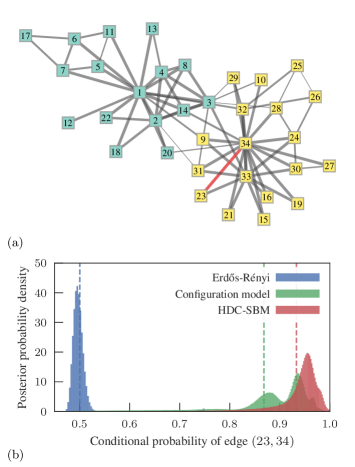
Figure 3: Inferred Zachary’s karate club network using the uncertain data from the original publication Zachary (1977), which contains an ambiguous edge $(23,34)$, as explained in the text. (a) Layout of the reconstructed network showing the posterior edge probabilities as edge thickness, according to the HDC-SBM, and the ambiguous edge in red. The node colors correspond to a sample from the posterior distribution of the node partitions. (b) Posterior probability density of the probability of edge $(23,34)$, conditioned on the remaining edges and model parameters, for the different model variants indicated in the legend and explained in the text. The vertical dashed lines indicate the distribution averages, corresponding to the marginal posterior probability of the edge.

In the following we move to a systematic analysis of the reconstruction method, based on empirical and simulated data.

II.3 Reconstruction performance

Before we evaluate the performance of the reconstruction approach, we must first decide how to quantify it. As a criterion of how close an inferred network $\hat{\bm{A}}$ is to the true network $\bm{A}^{*}$ underlying the data we will use the distance of Eq. 25,

$$d(\hat{\bm{A}},\bm{A}^{*})=\sum_{i<j}|\hat{A}_{ij}-A_{ij}^{*}|.$$

A successful reconstruction method should seek to find an estimate $\hat{\bm{A}}$ that minimizes this distance. However, since we do not have direct access to the true network $\bm{A}^{*}$, the best we can do is to consider the average distance over the posterior distribution given the noisy data,

$$\bar{d}(\hat{\bm{A}}) =\sum_{\bm{A}}d(\hat{\bm{A}},\bm{A})P(\bm{A}|\bm{x},\bm{n})$$ (41)

$$=\sum_{i<j}|\hat{A}_{ij}-\pi_{ij}|,$$ (42)

where

$$\pi_{ij}=\sum_{\bm{A}}A_{ij}P(\bm{A}|\bm{x},\bm{n}),$$ (43)

is the marginal posterior probability of edge $(i,j)$. If we minimize $\bar{d}(\hat{\bm{A}})$ with respect to $\hat{\bm{A}}$, we obtain

$$\hat{A}_{ij}=\begin{cases}1&\text{ if }\pi_{ij}>1/2\\ 0&\text{ if }\pi_{ij}<1/2,\end{cases}$$ (44)

for $\pi_{ij}\neq 1/2$. Eq. 44 defines what is called a maximum marginal posterior (MMP) estimator, and it leverages the consensus of the entire posterior distribution of all possible networks for the estimation of every edge. Operationally, it can be obtained very easily by sampling networks from the posterior distribution, and computing how often each edge is observed, yielding an estimate for $\bm{\pi}$ and hence $\hat{\bm{A}}$.

Given the above criterion, we evaluate the reconstruction performance by simulating the noisy measurement process. We do this by taking a real network $\bm{A}^{*}$ (which for this purpose we are free to declare to be error free), and obtaining a measurement $\bm{x}$ given error rates $p$ and $q$, and measuring each edge and nonedge the same number of times $n_{ij}=n$. We choose $p$ arbitrarily and $q=pE/[{N\choose 2}-E]$, where $E$ is the number of edges in $\bm{A}^{*}$, so that the measured networks have the same average density as $\bm{A}^{*}$. Given a final measurement $\bm{x}$, we sample inferred networks $\bm{A}$ from the posterior distribution $P(\bm{A}|\bm{x},\bm{n})$ and compute the MMP estimate $\hat{\bm{A}}$ from the marginal distribution $\bm{\pi}$. The quality of the reconstruction is then assessed according to the similarity to the true network $\bm{A}^{*}$, $S(\hat{\bm{A}},\bm{A}^{*})\in[0,1]$, defined as

$$S(\hat{\bm{A}},\bm{A}^{*})=1-\frac{d(\hat{\bm{A}},\bm{A}^{*})}{\sum_{i<j}\hat{A}_{ij}+A_{ij}^{*}},$$ (45)

where $d(\hat{\bm{A}},\bm{A}^{*})$ is the distance defined in Eq. 25. A value of $S(\hat{\bm{A}},\bm{A}^{*})=1$ indicates perfect reconstruction, and $S(\hat{\bm{A}},\bm{A}^{*})=0$ the situation where $\hat{\bm{A}}$ and $\bm{A}^{*}$ do not share a single edge.

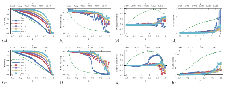
Figure 4: Reconstruction performance for political blogs (top row) and openflights (bottom row) networks. In each case, the empirical network was considered as the true network, and simulated measurements were made for several values of missing edge probability $p$, with a spurious edge probability $q=pE/[{N\choose 2}-E]$. [(a) and (e)] Similarity of the MMP estimator to the true network, $S(\hat{\bm{A}},\bm{A}^{*})$, as a function of $p$, and for several values of the number of repeated measurements, $n$. [(b), (c), (f), and (g)] Posterior average local clustering and degree assortativity coefficients, according to the same legend as (a) and (e). [(d) and (g)] KL divergence between true and inferred degree distributions, as discussed in the text. In all cases [(a) to (h)] the dashed curve shows the corresponding value obtained directly with the measured data with $n=1$, and the solid horizontal line marks the true value corresponding to perfect reconstruction.

In Figs. 4a and e are shown the results of this procedure with the political blogs and openflights networks (see Appendix E). As a baseline, in both figures we show the direct similarity $S(\bm{x},\bm{A}^{*})$ of the data obtained with $n=1$ to the true network $\bm{A}^{*}$, as dashed curves. In both cases the similarity of the inferred network $S(\hat{\bm{A}},\bm{A}^{*})$ to the true network is larger than the one obtained with the direct observation $S(\bm{x},\bm{A}^{*})$ for the vast majority of the parameter range, indicating systematic positive reconstruction even with single measurements. Expectedly, the quality of reconstruction increases progressively with a larger number of measurements $n$, with the similarity eventually approaching one. Although perfect reconstruction is not possible with single measurements when the noise is large, it is a noteworthy and nontrivial fact that the distance to the true network always decreases when performing it. This is only possible due to the use of a structured model such as the HDC-SBM that can recognize the structure in the data and extrapolate from it. If one would use a fully random model in its place, the similarity would be zero in the entire range, if $n=1$ (although it would improve for $n>1$).

A particularly interesting outcome of the successful reconstruction is that the noise magnitudes $p$ and $q$ can be determined as well, even though they are not a priori known. As shown in Fig. 5 the posterior probability for $p$ and $q$ are very close to the true values used, even for single measurements. (The precision of the inferred values of $q$ is generally higher than of $p$, as we are dealing with sparse networks, with vastly more nonedges than edges.) For the openflights data the accurate noise recovery only occurs for moderate magnitudes, and a strong discrepancy is observed for values around $p\gtrsim 0.5$. In such situations, prior knowledge of the noise values could have aided the reconstruction for $n=1$, but otherwise any benefit from this information would have been marginal. Again, the noise recovery becomes asymptotically exact as we increase the number of measurements, and is already very accurate for $n=2$.

We note that the results of Fig. 4 remain largely unchanged if the underlying network considered is sampled from the DC-SBM with parameters inferred from the original data (not shown).

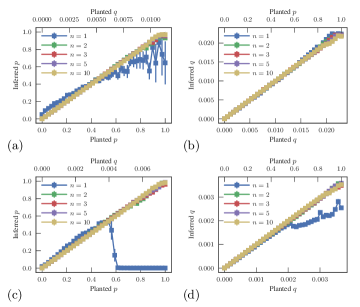
Figure 5: Inferred values of noise magnitude $p$ and $q$ as a function of the planted values, for the same simulated measurements described in Fig. 4, for the political blogs [(a) and (b)] and openflights [(c) and (d)] networks.

II.3.1 Estimating summary quantities

In addition or instead of the network itself, we may want to estimate a given scalar observable $y(\bm{A})$ that acts as a summary of some aspect of the network’s structure. In this case, we should seek to minimize the squared error with respect to the true network $\bm{A}^{*}$,

$$(\hat{y}-y(\bm{A}^{*}))^{2},$$ (46)

where $\hat{y}$ is our estimated value. Like before, without knowing $\bm{A}^{*}$ the best we can do is minimize the squared error averaged over the posterior distribution,

$$\sigma_{\hat{y}}^{2}=\sum_{\bm{A}}(\hat{y}-y(\bm{A}))^{2}P(\bm{A}|\bm{n},\bm{x}).$$ (47)

Minimizing $\sigma_{\hat{y}}^{2}$ with respect to $\hat{y}$ yields the posterior mean estimator,

$$\hat{y}=\sum_{\bm{A}}y(\bm{A})P(\bm{A}|\bm{n},\bm{x}).$$ (48)

We can also obtain the uncertainty of this estimator by computing its variance of Eq. 47, so that the uncertainty of $\hat{y}$ is summarized by its standard deviation, $\sigma_{\hat{y}}$.

It is important to emphasize that in general $\hat{y}\neq y(\hat{\bm{A}})$, with $\hat{\bm{A}}$ being the MMP estimator of Eq. 44. In other words, the best estimate for $y(\bm{A}^{*})$ (i.e. with minimal squared error) is not the same as the value obtained for the best estimate of $\bm{A}^{*}$ (i.e. with minimal distance).

In Figs. 4b, c, f, and g we see the results of the same experiment described above, where we attempt to recover the average local clustering coefficient and the degree assortativity of the original network. As with the similarity, the inferred values are closer to the true network’s. However, in this case the values for $n=1$ are substantially closer to the true value for a large range of noise magnitudes, and is often indistinguishable from it. This means that even in situations where the posterior distribution of inferred networks yields a relatively poor similarity to the true network, as it cannot precisely correct the altered edges and nonedges, it still shares a high degree of statistical similarity with it, and can accurately reproduce these summary quantities.

II.3.2 Estimating degree distributions

We can also estimate degree distributions $\hat{p}_{k}$, defined as the probability that a node has degree $k$, by treating them like a collection of scalar measurements, and minimize the squared error $\sum_{k}(\hat{p}_{k}-p_{k}(\bm{A}))^{2}$ averaged over the posterior distribution, which yields the same posterior mean estimator used so far,

$$\hat{p}_{k}=\sum_{\bm{A}}p_{k}(\bm{A})P(\bm{A}|\bm{x},\bm{n}).$$ (49)

The same estimator is also obtained when minimizing the Kullback-Leibler (KL) divergence,

$$\operatorname{KL}(p(\bm{A})||\hat{p})=\sum_{k}p_{k}(\bm{A})\ln\frac{p_{k}(\bm{A})}{\hat{p}_{k}},$$ (50)

over the posterior, which offers a more convenient way to compare distributions, as it can be interpreted as the amount of information “lost” when $\hat{p}_{k}$ is used to approximate $p_{k}(\bm{A})$.

For the estimation of the degree probabilities $p_{k}(\bm{A})$ for each individual network sampled from the posterior, we model the degrees $\bm{k}=\{k_{i}\}$ as a multinomial distribution

$$P(\bm{k}|\{p_{k}\})=\frac{N!\prod_{k}p_{k}^{n_{k}}}{\prod_{k}n_{k}!},$$ (51)

where $n_{k}$ is the number of nodes of degree $k$. The probabilities themselves are modelled by a uniform Dirichlet mixture, i.e., sampled uniformly from a simplex constrained by the normalization $\sum_{k=0}^{K}p_{k}=1$,

$$P(\{p_{k}\})=K!\delta\left(\textstyle\sum_{k}p_{k}-1\right),$$ (52)

where $K$ is the largest possible degree. With this, the the posterior mean becomes

$$p_{k}(\bm{A})=\frac{n_{k}+1}{N+K+1}.$$ (53)

This estimation is superior to the more naive $p_{k}=n_{k}/N$, as it is less susceptible to statistical fluctuations due to lack of data, such as when $n_{k}=0$, although it approaches it for $N\gg K$ and $n_{k}\gg 1$.

In Figs. 4d and h are shown the KL divergence between the inferred and true distributions, for the same experiments as before. Like with the local clustering and assortativity coefficients, the reconstructed degree distributions remain very close to the true one, despite the continuously decreasing similarity for larger noise magnitudes. In Fig. 6 can be seen the true, measured and reconstructed distributions for the political blogs network, for a value of $(p,q)=(0.41,0.0094)$. Despite the relatively high noise magnitudes, a single measurement of the network does fairly well in reconstructing the original distribution, failing mostly only for degrees zero and one, despite the significant distortion caused by the noisy measurement process.

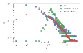
Figure 6: True, measured (with $n=1$) and reconstructed degree distributions of the political blog network, with noise magnitudes $(p,q)=(0.41,0.0094)$.

II.3.3 Edge prediction: network de-noising and completion

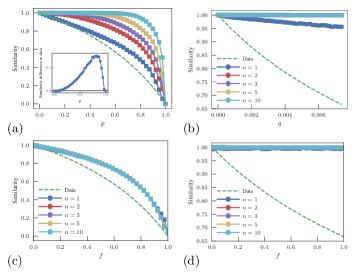
Figure 7: (a) Edge de-noising reconstruction performance for the openflights data, as a function of the missing edge probability $p$, for various $n$, and $q=0$. The dashed curve shows the corresponding value obtained directly with the measured data with $n=1$, and the inset shows the difference between the curve for $n=1$ and the dashed curve. (b) Same as (a) but for nonedge de-noising, with $p=0$. The values of $q$ were chosen to yield the same number of affected nonedges as edges in (a). (c) Edge completion reconstruction performance as a function of fraction $f$ of unobserved edges. The dashed line shows the value of similarity obtained by considering the unobserved edges as nonedges. (d) Same as (c) but for nonedge completion, as a function of the fraction $f$ of unobserved nonedges. The dashed line shows the value of similarity obtained by considering the unobserved nonedges as edges.

The reconstruction task we have been considering shares many similarities with the task of model-based edge prediction Clauset et al. (2008); Guimerà and Sales-Pardo (2009), but is also different from it in some fundamental aspects. Most typically, edge prediction is formulated as a binary classification task Lü and Zhou (2011), in which to each missing (or spurious) edge is attributed a “score” (which may or may not be a probability), so that those that reach a pre-specified discrimination threshold are classified as true edges (or true nonedges). This threshold is an input of the procedure, and usually the quality of the classification is assessed by integrating the true positive rate versus the false positive rate [a.k.a. the Receiver Operating Characteristic (ROC) curve] for all discrimination threshold values. This yields the Area Under the Curve (AUC), which lies in the unit interval, and can be equivalently interpreted as the probability that a randomly selected true positive will be ranked above a randomly chosen true negative. Thus, a value of $1/2$ indicates a performance equivalent to a random guess, and a value of $1$ indicates “perfect” classification (note that a classifier with AUC value of $1$ still requires the correct discrimination threshold as an input to fully recover the network).

In contrast, the reconstruction task considered here yields a full posterior distribution $P(\bm{A}|\bm{n},\bm{x})$ for the inferred network $\bm{A}$. Although this can be used to perform the same binary classification task, by using the posterior marginal probabilities $\pi_{ij}$ as the aforementioned “scores,” it contains substantially more information. For example, the number of missing and spurious edges (and hence the inferred probabilities $p$ and $q$) are contained in this distribution, and thus do not need to be pre-specified. Indeed, our method lacks any kind of ad hoc input, such as a discrimination threshold (note that the threshold $1/2$ in the MMP estimator of Eq. 44 is a derived optimum, not an input). This means that absolute assessments such as the similarity of Eq. 45 can be computed instead of relative ones such as the AUC.

Furthermore, the reconstruction approach can be used to recover summary quantities and perform error estimates, which is usually not directly possible in the binary classifier framing. In addition, reconstructed networks can contain spurious and missing edges simultaneously, whereas with traditional edge prediction methods, they each require their own binary classification (with their own discrimination thresholds).

When doing edge prediction, one often distinguishes recovering from the effects of noise (i.e. an edge has been transformed into a nonedge, or vice versa) — to which we refer as de-noising — and from a lack of observation (i.e. a given entry in the adjacency matrix is unknown) — to which we refer as completion. In each scenario the scores are computed differently, yielding different classifiers. When performing reconstruction with our method, we inherently allow for any arbitrary combination of de-noising and completion: if an entry is not observed, it has a value of $n_{ij}=0$, which is different from it being observed with $n_{ij}>0$ as a nonedge $x_{ij}=0$. If the noise parameters $p$ and $q$ are zero, recovery via the posterior distribution amounts to a pure completion task for the entries with $n_{ij}=0$, and likewise we have a pure de-noising task if $n_{ij}>0$ for every pair $(i,j)$, otherwise we have a mixture of these two tasks.

In Fig. 7 we illustrate some of these tasks, performed using our framework for the openflights dataset, which we found to be representative of the majority investigated. In Fig. 7a and b are shown the results for edge ($q=0$) and nonedge ($p=0$) de-noising, respectively. Given that this network is sparse, the probability of an edge is on average much smaller than that of a nonedge, which means that the edge de-noising task is significantly harder than nonedge de-noising, for which very high accuracy can be obtained even for $n=1$ measurement per edge. Nevertheless, positive reconstruction is possible in each case, approaching a similarity of $1$ as the number of measurements is increased.

We also perform network completion by choosing a fraction $f$ of edges or nonedges, for which zero measurements are performed, $n_{ij}=0$, while the remaining entries are observed $n$ times, $n_{ij}=n$. In Fig. 7c and d are shown the reconstruction results for edge and nonedge completion, respectively. Like for de-noising, nonedge completion is easier, approaching near perfection for the entire range of parameters, and for the same reason as before. For the completion tasks, however, the number of observations $n$ for the non-affected entries has a negligible effect in the reconstruction, and we observe near-optimal performance already for $n=1$.

Although the number of edges and nonedges affected is the same for both our de-noising and completion examples, the latter yields a larger rate of successful reconstruction for both edges and nonedges. This is understood by noting that these tasks have a different number of unknowns. In the case of edge completion, on the one hand, for a given finite fraction $f$ of non-observed edges, we have $O(E)$ unknowns, which for sparse networks is $O(N)$. For edge de-noising, on the other hand, for any fraction $p$ of missing edges, for sparse networks we have in principle $O(N^{2})$ possibilities for their placements, corresponding to all observed nonedges. For nonedge de-noising and completion, the difficulty is comparable: For any fraction $f=O(1/N)$ left unobserved, or $q=O(1/N)$ transformed into spurious edges, there are $O(N)$ unknowns, if the network is sparse. However, the actual number of unknowns for nonedge completion is strictly smaller, as it must involve only the fraction not observed, whereas for de-noising it involves every observed edge.

This difference in performance shows how the correct interpretation of the data can be crucial — as absence of evidence is not evidence of absence. Unfortunately, most available datasets fail to make this distinction, including those few which actually provide some amount of error assessments, as they do not indicate which pairs of nodes have not been measured at all.

II.3.4 Detectability of modular structures

Figure 8: (a) Normalized mutual information (NMI) between planted and inferred partitions for a PP model with $N=10^{4}$, $B=2$, ${\left<k\right>}=10$, and measurement errors $q=0$ and $p$ given in the legend, together with the number of measurements $n$. The black solid line marks the threshold of Eq. 55, and the blue dashed line the threshold of Eq. 56 with $(p,q)=(1/2,0)$. (b) Same as in (a), but for the similarity $S(\hat{\bm{A}},\bm{A}^{*})$ between the inferred and true networks.

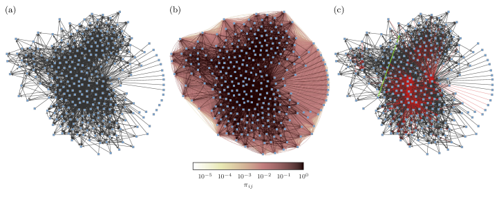
Figure 9: (a) Measured neural network of the C. elegans worm White et al. (1986). (b) Marginal posterior distribution $\pi_{ij}$ of the edges according to our reconstruction method, shown as edge colors. (c) Maximum marginal posterior (MMP) estimate of the network, with inferred missing edges shown in red, and spurious edges shown in green.

Our approach generalizes the task of community detection for networks with measurement errors. However, even in the case of error-free networks with planted community structure, this task is not always realizable. This is most often illustrated with a simple SBM parametrization known as the planted partition model (PP),

$$\omega_{rs}=\omega_{\text{in}}\delta_{rs}+\omega_{\text{out}}(1-\delta_{rs}),$$ (54)

with equal-sized groups, $n_{r}=N/B$. As has been shown in Ref. Decelle et al. (2011), the detection of communities from networks sampled from this model undergoes as phase transition, and becomes impossible for parameter values satisfying

$$N|\omega_{\text{in}}-\omega_{\text{out}}|<B\sqrt{{\left<k\right>}},$$ (55)

where ${\left<k\right>}=N[\omega_{\text{in}}+(B-1)\omega_{\text{out}}]/B$ is the average degree of the network. This transition means that even though a PP model may contain assortative community structure with $\omega_{\text{in}}>\omega_{\text{out}}$, the individual samples from the generative model will be indistinguishable from a fully random graph if the inequality of Eq. 55 is fulfilled, and hence will contain no information useful for the recovery of the planted communities.

When considering measured networks, it is expected that the introduced errors will make the detection task more difficult, as the noise will remove information from the data. As we have seen in Sec. II.1.1, when a single measurement of a SBM network is made with noise parameters $p$ and $q$, it becomes indistinguishable from a SBM sample with effective probabilities $\bm{\omega}^{\prime}$, given by Eq. 36. Applying this to the PP model, yields a transition according to

$$N|\omega_{\text{in}}-\omega_{\text{out}}|<\frac{B\sqrt{(1-p-q){\left<k\right>}+qN}}{(1-p-q)}.$$ (56)

For positive error magnitudes $p>0$ or $q>0$, the above threshold will be larger than Eq. 55. This highlights how measurement noise can hinder the detection of large-scale structures if they are sufficiently weak, and induce a phase transition in their detection. This also means that the reconstruction of the networks themselves will be affected by the same transition, as our approach hinges on the detectability of these large-scale structures.

In Fig. 8 are shown the reconstruction results for PP network samples with $B=2$ groups, for simulated measurements always using $q=0$, but with either $p=0$ or $p=1/2$. Without measurement noise, $p=0$, the detectability of the planted partition is possible all the way down to the detectability threshold of Eq. 55. Despite the lack of noise, the similarity with the true network is only slightly above $0.6$ in the detectable region. This is because the probabilities in this ensemble are not sufficiently heterogeneous to rule out high noise values, as some of the empirical networks we have considered. Below the transition, the similarity falls to zero, as the network becomes indistinguishable from a fully random one. Interestingly, this partial uncertainty about the network does not affect the inference of the node partition. If we increase the noise to $p=1/2$, the partition recovery is possible up to the threshold of Eq. 56 when only $n=1$ measurements are made. However, after sufficiently increasing $n$, the effects of noise are diminished, and the original threshold can be achieved. In this case, the similarity also becomes high even below the detectability threshold, where the community structure itself cannot be recovered. This is because the repeated measurements themselves yield sufficient information about the network structure, and the reconstruction no longer needs to rely on the network structure itself.

II.4 Reconstruction of empirical data and uncertainty assessment

A central advantage of our method is that it can be used to reconstruct noisy networks when only a single measurement has been made for each entry in the adjacency matrix, and no error assessment is known. As the majority of network data can be cast into this framework, our method can be used to reconstruct them and give uncertainty assessments for quantities of interest. In this section we discuss a few empirical examples.

We focus first on the neural network of the Caenorhabditis elegans worm. It has been used extensively as a model organism, and it had its full neural network mapped in 1986 by White et al White et al. (1986). The network measurement has been done by electron microscopy of transverse serial sections of the animal’s body of about 50 nm thickness, amounting to around 8000 images. Based on these images, the network was reconstructed by painstaking manual tracing of the neuron paths across the different images. The reliability of the reconstruction procedure was discussed in Ref. White et al. (1986), where human error in tracing the neuron bundles, the orientation of the neurons with respect to the transverse section, and poor image quality were identified as the main sources of potential errors. White et al. employed a series of error mitigating procedures, such as detecting basic connection inconsistencies, exploiting the partial bilateral symmetry for suspect connections, and comparing with independent reconstructions of parts of the network. Although the authors of that work profess to be “reasonably confident” that the structure they present is “substantially correct,” they do not exclude the possibility of remaining errors, nor do they quantify in any way the uncertainty of their measurements. Furthermore, the data commonly used for network analysis, which we also use here, has been manually compiled by Watts et al. Watts and Strogatz (1998), based on the original data of Ref. White et al. (1986), and may contain further errors. The resulting data we use amount to $N=302$ nodes and $E=2,345$ directed edges (note that five nodes were excluded in Ref. Watts and Strogatz (1998) for not having any connections. We include these nodes in our analysis, as it is suspicious that isolated neurons can exist, and thus is probably a symptom of missing data).

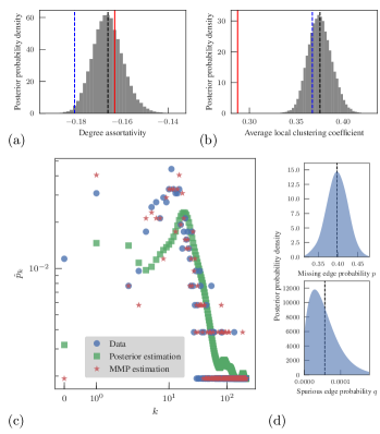
Figure 10: Reconstruction statistics for the neural network of C. elegans. (a) Posterior distribution of the degree assortativity coefficient. The black dashed line marks the mean of the distribution, and the blue dashed line the value obtained for the MMP estimate, $\hat{\bm{A}}$. The red solid line marks the value computed directly from the data. (b) Same as (a) but for the average local clustering coefficient. (c) Measured and estimated degree distributions. (d) Posterior distributions for the error probabilities $p$ and $q$.

When we employ our reconstruction procedure on the C. elegans data, we find the results shown in Figs. 9 and 10, and summarized in Table 1. The MMP estimate of this network contains $\hat{E}=2,773$ edges, but the posterior distribution is significantly broad, and contains on average ${\left<E\right>}=3,950$ edges, meaning that there are many potential edges with low but non-negligible probabilities. We note that our reconstruction connects the isolated nodes in the data to the main hub in the network, which is an important neuron situated in the head of the worm. As seen in Fig. 10a the inferred degree assortativity coefficient is compatible with the value measured directly from data, and our method is capable of providing a confidence interval for this estimation. The same is not true for the average local clustering coefficient, as seen in Fig. 10b, which is not compatible with the value measured directly from data with any reasonable confidence.

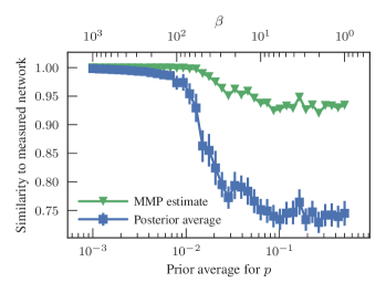
Figure 11: Average similarity between the posterior samples and the measured C. elegans data as function of the hyperparameter $\beta$ (with $\alpha=1$), which controls the prior belief on the probability $p$ of missing edges (the average of which is shown in the x axis). For reference, the similarity for the MMP estimate is also shown.

For the C. elegans data, the inferred error rates are $(\hat{p},\hat{q})=(0.4,6\times 10^{-5})$. Although this corresponds to a very high accuracy with respect to spurious edges, it indicates a low accuracy with respect to missing edges, and it implies that almost half of the original edges were misrepresented as nonedges. Although the consensus of the posterior distribution (represented by the MMP estimate) is reasonably close to the original data, with a similarity of $0.93$, the similarity averaged over the posterior distribution is only $0.74$ indicating a fair amount of uncertainty. This seems to contradict the qualitative assessment of Ref. White et al. (1986), which argued in favor of the reliability of their data. This discrepancy can be interpreted in two ways: 1. The assessment in Ref. White et al. (1986) was too optimistic, and the data contains indeed more errors than anticipated; 2. The data actually contains fewer errors than our method predicts, but the true network itself is not sufficiently structured to rule out errors in a manner that can be exploited by our method. However, even if case 2 happens to be true, our method correctly projects an agnostic prior assumption about the error rates onto the posterior distribution, after being informed by the data. This means that more confidence on the data and the existence of fewer errors must be accompanied by either more data (e.g. repeated measurements), or a more refined prior information on the error rates, obtained either by calibration or a quantitative study of the methods employed in Ref. White et al. (1986). As an illustration, in Fig. 11 is shown the posterior similarity with the date obtained with different choices of the hyperparameter $\beta$, using $\alpha=1$, which control the prior knowledge on the value of $p$, with an average given by ${\left<p\right>}=\alpha/(\alpha+\beta)$. A high accuracy of the data, with inferred similarities approaching one, is only achieved by a prior belief on $p$ being on the order of $0.01$ or smaller. This means that one should trust the claimed high accuracy in Ref. White et al. (1986) only if one is confident that the probability of an edge not being recognized as such was below one percent. This might very well be true, but would need to be substantiated with further evidence. Although in situations such as these our method cannot fully resolve the discrepancy without further data, it serves as the appropriate framework in which to place the issue, and shows that any analysis that takes the original measured data for granted, ignoring potential errors, inherently assumes more reliability than can be inferred from the data alone.

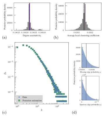
Figure 12: Reconstruction statistics for the co-authorship network of arxiv.org. (a) Posterior distribution of the degree assortativity coefficient. The black dashed line marks the mean of the distribution, and the blue dashed line the value obtained for the MMP estimate, $\hat{\bm{A}}$. The red solid line marks the value computed directly from the data. (b) Same as (a) but for the average local clustering coefficient. (c) Measured and estimated degree distributions. (d) Posterior distributions for the error probabilities $p$ and $q$.

For other kinds of data, it is possible to obtain very accurate reconstructions with single measurements. As an example, we consider the network of collaborations in papers published in the cond-mat section of the arxiv.org pre-print website in the period spanning from January 1, 1995 and March 31, 2005, where authors are nodes, and an edge exists if two authors published a paper together Newman (2001). This network was compiled by crawling through the website interface, and could contain errors due to incorrect parsing. When reconstructed using our method, however, we find that it is remarkably accurate, with very low error rates inferred as $(p,q)=(3\times 10^{-5},3\times 10^{-9})$. As can be seen in Fig. 12, all inferred properties match very closely the direct measurement — although our reconstruction is still useful in providing error estimates for them.

In Table 1 we provide a summary of reconstruction results with our method to several empirical networks. We observe a tendency of larger networks to be more accurate than smaller ones. This is not a trivial result of there being more data, but rather of these larger networks containing stronger structures which are informative of low measurement noise. If these networks were fully random, their reconstruction accuracy would have been very poor, regardless of their size.

Dataset	Similarity	Nodes	Edges		Degree assortativity		Local clustering		$B_{e}$	$\hat{p}$	$\hat{q}$
			Direct	Estimated	Direct	Estimated	Direct	Estimated
Karate club	$0.94(4)$	$34$	$78$	$77(7)$	$-0.475\,613\,097\,7$	$-0.49(5)$	$0.570\,638\,478\,2$	$0.58(5)$	$2.7(6)$	$0.06(5)$	$0.012(10)$
9/11 terrorists	$0.96(2)$	$62$	$152$	$154(8)$	$-0.080\,475\,661\,8$	$-0.096(20)$	$0.486\,371\,555\,9$	$0.50(2)$	$5.4(5)$	$0.05(4)$	$0.003(2)$
American football	$0.857(16)$	$115$	$613$	$500(18)$	$0.162\,442\,249\,6$	$0.18(7)$	$0.403\,216\,011$	$0.68(4)$	$12.7(3)$	$0.05(3)$	$0.0226(19)$
Network scientists	$0.9981(17)$	$379$	$914$	$915(3)$	$-0.081\,677\,848\,3$	$-0.0823(18)$	$0.741\,230\,614\,3$	$0.741(3)$	$29.6(14)$	$0.004(3)$	$3.1(19)\text{\times}{10}^{-5}$
C. elegans neural	$0.744(19)$	$302$	$2345$	$3950(160)$	$-0.163\,199\,210\,3$	$-0.167(7)$	$0.287\,522\,845\,9$	$0.378(12)$	$17.0(3)$	$0.41(2)$	$6(3)\text{\times}{10}^{-5}$
Malaria genes	$0.9981(15)$	$1103$	$2965$	$2973(9)$	$-0.300\,132\,763\,2$	$-0.2997(20)$	$0$	$0(0)$	$30.8(3)$	$0.004(3)$	$4(3)\text{\times}{10}^{-6}$
Power grid	$0.80(7)$	$4941$	$6594$	$9900(1300)$	$0.003\,456\,987\,7$	$0.043(17)$	$0.080\,103\,611\,1$	$0.058(7)$	$15.6(7)$	$0.33(10)$	$2.5(19)\text{\times}{10}^{-7}$
Political blogs	$0.965(5)$	$1222$	$16\,714$	$17\,860(190)$	$-0.221\,328\,723$	$-0.2226(16)$	$0.320\,254\,619\,4$	$0.343(5)$	$16.6(3)$	$0.066(10)$	$4.4(17)\text{\times}{10}^{-5}$
DBLP citations	$0.64(1)$	$12\,590$	$49\,744$	$106\,000(2000)$	$-0.045\,724\,583\,3$	$-0.0559(19)$	$0.117\,183\,554\,4$	$0.164(7)$	$86.4(20)$	$0.529(11)$	$9(5)\text{\times}{10}^{-9}$
Openflights	$0.9916(9)$	$3286$	$39\,430$	$40\,100(70)$	$-0.005\,311\,689\,7$	$-0.0071(11)$	$0.496\,468\,558\,8$	$0.507(2)$	$117.1(5)$	$0.0167(18)$	$1.0(3)\text{\times}{10}^{-7}$
Reactome	$0.999\,977(10)$	$6327$	$146\,160$	$146\,164(3)$	$0.244\,874\,480\,9$	$0.244\,87(4)$	$0.588\,375\,016$	$0.5887(3)$	$318.7(10)$	$4.1(18)\text{\times}{10}^{-5}$	$1.3(8)\text{\times}{10}^{-7}$
cond-mat	$0.999\,986(13)$	$40\,421$	$175\,693$	$175\,695(4)$	$0.186\,326\,578\,9$	$0.186\,33(2)$	$0.636\,159\,643\,3$	$0.636\,15(3)$	$1014(6)$	$3(2)\text{\times}{10}^{-5}$	$3(2)\text{\times}{10}^{-9}$
Enron email	$0.999\,86(5)$	$36\,692$	$183\,831$	$183\,885(18)$	$-0.110\,764\,032\,6$	$-0.110\,75(2)$	$0.496\,982\,559\,6$	$0.496\,92(8)$	$188.9(11)$	$0.000\,28(10)$	$2.9(19)\text{\times}{10}^{-9}$
Linux source	$0.9973(3)$	$30\,837$	$213\,424$	$214\,600(120)$	$-0.174\,678\,974\,1$	$-0.174\,67(7)$	$0.128\,491\,999$	$0.1322(10)$	$351.2(7)$	$0.0055(5)$	$1.7(10)\text{\times}{10}^{-9}$
Brightkite	$0.9985(3)$	$58\,228$	$214\,078$	$214\,740(80)$	$0.010\,815\,796\,3$	$0.011\,00(11)$	$0.172\,325\,927\,4$	$0.172\,34(10)$	$151(3)$	$0.0029(5)$	$1.7(12)\text{\times}{10}^{-8}$
PGP	$0.997\,99(9)$	$39\,796$	$301\,498$	$301\,660(60)$	$0.000\,757\,492\,8$	$0.000\,49(8)$	$0.461\,087\,299\,3$	$0.4617(2)$	$929(2)$	$0.002\,27(16)$	$3.35(18)\text{\times}{10}^{-7}$
Internet AS	$0.999\,67(13)$	$53\,387$	$496\,731$	$497\,070(130)$	$-0.186\,967\,455\,5$	$-0.186\,959(17)$	$0.680\,968\,528\,1$	$0.681\,26(14)$	$218.0(16)$	$0.0007(3)$	$1.0(8)\text{\times}{10}^{-9}$
Web Stanford	$0.999\,998\,7(8)$	$281\,903$	$2\,312\,497$	$2\,312\,494(4)$	$-0.112\,444\,517\,4$	$-0.112\,444\,7(2)$	$0.597\,630\,460\,8$	$0.597\,634(3)$	$4168(2)$	$1.0(2)\text{\times}{10}^{-6}$	$7(5)\text{\times}{10}^{-11}$
Flickr	$0.999\,976(13)$	$105\,938$	$2\,316\,948$	$2\,316\,830(60)$	$0.246\,851\,188\,3$	$0.246\,823(16)$	$0.089\,128\,022\,7$	$0.089\,138(7)$	$617(2)$	$6(3)\text{\times}{10}^{-7}$	$2.0(11)\text{\times}{10}^{-8}$

Table 1: Reconstruction results for empirical networks with single measurements per edge, and no available primary error assessments. Similarity refers to the average of $S(\bm{A},\bm{A}^{*})$ over the posterior distribution. For each quantity (number of edges, degree assortativity, average local clustering) is shown the value directly obtained from the data (direct) and the average over the posterior distribution (estimated). The value of $B_{e}$ is the posterior average of the effective number of inferred communities $e^{H(\bm{n})}$, with $H(\bm{n})=-\sum_{r}(n_{r}/N)\ln(n_{r}/N)$, where $n_{r}$ is the number of nodes in group $r$, being the entropy of the group size distribution. The values $\hat{p}$ and $\hat{q}$ are the posterior averages of the error rates. In all cases, the parentheses indicate the standard deviation over the posterior distribution. Dataset descriptions are given in Appendix E.

II.5 Heterogeneous errors

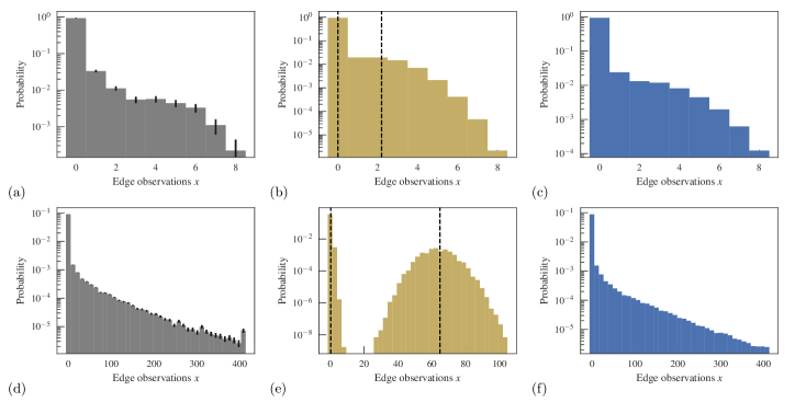
Figure 13: Distribution of edge occurrences, $x_{ij}$, for the reality mining (top row) and human connectome (bottom row) datasets. [(a) and (d)] Empirical data. [(b) and (e)] Generated from inferred parameters, according to the uniform model. [(c) and (f)] Generated from inferred parameters, according to the nonuniform model.

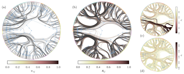
Figure 14: Reconstruction results for the human connectome. (a) Marginal posterior distribution of edges $\pi_{ij}$ and inferred hierarchical partition, according to the model with uniform errors. The upper hierarchy branch corresponds to the right hemisphere. (b) Same as (a) but with the nonuniform model. (c) Inferred missing edge probabilities $p_{ij}$ for the nonuniform model. (d) Same as (c) but for the spurious edge probabilities, $q_{ij}$.

So far we have considered only the situation where the error probabilities $p$ and $q$ are the same for every pair of nodes in the network. Although it is easy to imagine a simplified scenario where the same measurement instrument is used in every case, it is also easy to imagine situations where this is not an adequate representation of how measurement is made. For example, in the case of the C. elegans neural network, the spatial proximity of the neurons may make it harder or easier to measure the edges and nonedges, thus impacting their error probabilities.

With this in mind, it is easy to generalize our framework to allow for individual error probabilities $p_{ij}$ and $q_{ij}$, for missing and spurious edges between nodes $i$ and $j$, respectively. Given a true underlying entry $A_{ij}$ between these two nodes, its measurement probability is given by

$$P(x_{ij}|n_{ij},A_{ij},p_{ij},q_{ij})=\\ {n_{ij}\choose x_{ij}}\left[(1-p_{ij})^{x_{ij}}p_{ij}^{n_{ij}-x_{ij}}\right]^{A_{ij}}\times\\ \left[q_{ij}^{x_{ij}}(1-q_{ij})^{n_{ij}-x_{ij}}\right]^{1-A_{ij}}.$$ (57)

Using the same Beta priors as before, we can integrate over $p_{ij}$ and $q_{ij}$, obtaining

$$P(x_{ij}|n_{ij},A_{ij},\alpha,\beta,\mu,\nu)\\ =\int P(x_{ij}|n_{ij},A_{ij},p_{ij},q_{ij})P(p_{ij}|\alpha,\beta)P(q_{ij}|\mu,\nu)\;\mathrm{d}p_{ij}\mathrm{d}q_{ij}\\ ={n_{ij}\choose x_{ij}}\left[\frac{\mathcal{B}(n_{ij}-x_{ij}+\alpha,x_{ij}+\beta)}{\mathcal{B}(\alpha,\beta)}\right]^{A_{ij}}\times\\ \left[\frac{\mathcal{B}(x_{ij}+\mu,n_{ij}-x_{ij}+\nu)}{\mathcal{B}(\mu,\nu)}\right]^{1-A_{ij}}.$$ (58)

With this we have the full conditional distribution for the measured network,

$$P(\bm{x}|\bm{n},\bm{A},\alpha,\beta,\mu,\nu)=\prod_{i<j}P(x_{ij}|n_{ij},A_{ij},\alpha,\beta,\mu,\nu)$$ (59)

with which we can obtain the posterior distribution of Eq. 3. However, unlike the case with uniform errors, the choice of hyperparameters is now vital. The noninformative assumption $\alpha=\beta=\mu=\nu=1$ applied above makes the likelihood independent of the planted network $\bm{A}$, rendering the data completely uninformative as well. This means we must have some global information that specifies how the values of $p_{ij}$ and $q_{ij}$ are distributed. Although we could simply set (or fit) the values of the hyperparameters to values different from one, we favor a nonparametric approach, and we include the hyperparameters in the posterior distribution,

$$P(\bm{A},\bm{b},\alpha,\beta,\mu,\nu|\bm{n},\bm{x})=\\ \frac{P(\bm{x}|\bm{n},\bm{A},\alpha,\beta,\mu,\nu)P(\bm{A}|\bm{b})P(\bm{b})P(\alpha,\beta,\mu,\nu)}{P(\bm{x}|\bm{n})}$$ (60)

which requires their own hyperprior distribution $P(\alpha,\beta,\mu,\nu)$. Here we will be agnostic and use a constant prior $P(\alpha,\beta,\mu,\nu)\propto 1$, with an unspecified and unnecessary normalization constant, as it cancels out in the posterior distribution. The inference algorithm is the same as before, but in addition to move proposals for the network $\bm{A}$ and node partition $\bm{b}$, we make also move proposals for the hyperparameters.

Like in the uniform case, we can obtain the posterior distribution for the error probabilities via their conditional posteriors, i.e.

$$P(p_{ij}|n_{ij},x_{ij},A_{ij},\alpha,\beta)=\\ \frac{p^{A_{ij}(n_{ij}-x_{ij})+\alpha-1}(1-p)^{x_{ij}A_{ij}+\beta-1}}{\mathcal{B}(A_{ij}(n_{ij}-x_{ij})+\alpha,x_{ij}A_{ij}+\beta)}$$ (61)

and likewise for $q_{ij}$ with

$$P(q_{ij}|n_{ij},x_{ij},A_{ij},\mu,\nu)=\\ \frac{q^{(1-A_{ij})x_{ij}+\mu-1}(1-q)^{(1-A_{ij})(n_{ij}-x_{ij})+\nu-1}}{\mathcal{B}((1-A_{ij})x_{ij}+\mu,(1-A_{ij})(n_{ij}-x_{ij})+\nu)},$$ (62)

averaged over the posterior distribution.

We note that for heterogeneous error rates, the case with single measurements $n_{ij}=1$ become less interesting. If we replace $n_{ij}=1$ and $x_{ij}\in\{0,1\}$ in the above equations, they become identical to Eq. 15 for the case with uniform errors, if we make the substitution

$$p =\frac{\mathcal{B}(\alpha+1,\beta)}{\mathcal{B}(\alpha,\beta)}=\frac{\alpha}{\alpha+\beta},$$ (63)

$$q =\frac{\mathcal{B}(\mu+1,\nu)}{\mathcal{B}(\mu,\nu)}=\frac{\mu}{\mu+\nu}.$$ (64)

In this situation, only the prior averages of $p_{ij}$ and $q_{ij}$ matter, not their variance. A uniform prior for $\alpha,\beta,\mu$ and $\nu$ is equivalent to Beta priors with parameters $(1,0)$ for $p$ and $q$ computed via the equation above, and hence this approach becomes completely identical to the one with uniform errors considered before. Therefore, there is no sufficient data in the single measurement case to detect heterogeneous errors of this kind, and thus a meaningful use of this method is confined to data with $n_{ij}>1$. Note also that this implies that any error heterogeneity present in the data will be conflated with underlying network structure when single measurements are made. Ultimately, this conflation can only be resolved by making multiple measurements.

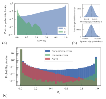
Figure 15: Inferred uncertainties for the human connectome. (a) Posterior distribution of $p_{ij}$ and $q_{ij}$, using the nonuniform model. (b) Posterior distribution of $p$ and $q$, using the uniform model. (c) Distribution of posterior marginal edge probabilities $\pi_{ij}$, according to both model variants, as well as the naive estimate $\tilde{\pi}_{ij}=x_{ij}/n_{ij}$.

Dataset	$n$	Nodes	Edges		Degree assortativity		Local clustering		$B_{e}$		$\hat{p}$		$\hat{q}$
			Uniform	Nonuniform	Uniform	Nonuniform	Uniform	Nonuniform	Uniform	Nonuniform	Uniform	Nonuniform	Uniform	Nonuniform
Karate club	$2$	$34$	$77.9(3)$	$95(6)$	$-0.475(3)$	$-0.43(5)$	$0.569(8)$	$0.63(5)$	$2.9(6)$	$2.9(6)$	$0.012(2)$	$0.49(3)$	$0.0011(3)$	$0.0004(13)$
Reality mining	$8$	$96$	$293(11)$	$280(20)$	$-0.23(3)$	$-0.23(3)$	$0.31(2)$	$0.29(2)$	$3.5(6)$	$3.4(6)$	$0.724(8)$	$0.71(3)$	$0.0007(2)$	$0.001(2)$
School friends	$6$	$2539$	$12\,500(40)$	$8200(300)$	$0.258(4)$	$0.322(6)$	$0.1535(13)$	$0.188(3)$	$82.5(3)$	$80.2(3)$	$0.5064(11)$	$0.16(3)$	$1.80(7)\text{\times}{10}^{-5}$	$0.0002(9)$
Human connectome	$418$	$1015$	$23\,020(16)$	$62\,000(6000)$	$0.0008(5)$	$0.002(3)$	$0.6796(4)$	$0.68(7)$	$100.5(11)$	$51.26(19)$	$0.845\,03(8)$	$0.93(9)$	$0.000\,984\,6(10)$	$1(11)\text{\times}{10}^{-4}$

Table 2: Reconstruction results for empirical networks with multiple measurements per edge. For each quantity is show the value obtained using either the uniform or the nonuniform model, as indicated. The value of $B_{e}=e^{H(\bm{n})}$ is the effective number of inferred communities, computed as $H(\bm{n})=-\sum_{r}(n_{r}/N)\ln(n_{r}/N)$, where $n_{r}$ is the number of nodes in group $r$. The values $\hat{p}$ and $\hat{q}$ are the posterior averages of the error rates. In all cases, the parentheses indicate the standard deviation over the posterior distribution. Dataset descriptions are given in Appendix E.

We consider two datasets which contain multiple measurements, in order to compare both approaches. We consider the reality mining dataset, which recorded proximity interactions between voluntary students over time Eagle and (Sandy). Following Ref. Newman (2018a), as measurements we considered the state of the network during eight consecutive Wednesdays in March and April of 2005, so chosen to avoid weekly periodic events. In addition, we consider the human connectome, using data from the Budapest Reference Connectome Szalkai et al. (2017) (which itself is based on primary data from the Human Connectome Project McNab et al. (2013)). This dataset contain records of the neuronal connections of $418$ individuals, each of which we considered as a separate measurement.

For both datasets considered — as it is arguably always true whenever multiple network measurements are made — it is debatable whether there is really a true single network behind the measurements, as our method assumes. For example, in the reality mining dataset, the underlying network could be changing over time, and the connectome can vary between individuals for physiological reasons, rather than measurement error. In each case, however, we are free to keep the mathematical structure of our model in place, and change its interpretation. We could, for instance, assume that the single network being inferred amounts simply to a consensus or a blue print of the network, and the “error” rates $p_{ij}$ and $q_{ij}$ indicate the variability of each single edge or nonedge around this blue print. Since both scenarios are generally conflated when making this kind of measurement, we can choose the interpretation that is most suitable according to the context.

In Fig. 13a and d are shown the distributions of the measured frequencies of edge occurrences, $x_{ij}$, for both datasets. For the human connectome, we observe a very broad distribution, with occurrences present in the entire possible range. In Fig. 13b and e we see the simulated results by sampling parameters from the posterior distribution and generating new data from them, using in this case the model with uniform errors. Whereas the results for reality mining are reasonably close to the data, the results for the human connectome show an obvious discrepancy, where the generated data is concentrated around two modes, corresponding to the frequencies of edges and nonedges. Indeed, for the uniform model this separation is guaranteed to occur for any given $p\neq 1/2$ and $q\neq 1/2$ and a sufficiently large number of measurements. The fact that this is not observed in the data is a clear indication that the error rates are not uniform (or alternatively, but mathematically equivalently, that there is no single network behind the measurements). Indeed when using the nonuniform model, it recovers the observed frequency almost perfectly, as seen in Figs. 13c and f.

If we look more closely at the human connectome data, we see that both approaches give us different pictures of the underlying network structure. As is summarized in Table 2, the uniform model yields a sparser network, which nevertheless seems more finely structured, with close to $100$ effective groups detected. Conversely, the nonuniform model yields a denser network, with a more uniform structure, and only half as many identified groups. In Fig. 14 we see more clearly the differences between both results. Both are capable of uncovering the hemispherical divisions and the partial bilateral symmetry of the connectome. The nonuniform model can detect a larger number of edges, but it yields larger probabilities of missing edges $p_{ij}$ which are heterogeneously distributed. In Fig. 14c it can be seen that the inferred $p_{ij}$ are strongly correlated with the detected group structure, and in particular seem to indicate a rather stable set of edges (low $p_{ij}$) that belong mostly to the left hemisphere. The uniform model, on the other hand, incorporates the variability of edge occurrences in the model itself, subdividing the groups further to accommodate it. Therefore, the nonuniform model gives a more faithful separation between the consensus and the variability around it.

In Fig. 15 we can see the posterior distributions of $p_{ij}$, $q_{ij}$ for the nonuniform model, as well $p$ and $q$ for the uniform model, showing how the former is indeed significantly more heterogeneous than the latter. In Fig. 15c is also shown the distribution of posterior probabilities $\pi_{ij}$ for both models, in addition to the naive estimate $\tilde{\pi}_{ij}=x_{ij}/n_{ij}$. This naive estimate is crude, as it does not differentiate between the different sources of error (spurious or missing edge), and does not take into account the observed correlations between the different entries. Indeed, as the Fig. 15c shows, it leads to very different results, which are not correctly justified, and should be avoided.

III Incorporating extrinsic uncertainty estimates

So far we have considered only situations where direct error estimates on the edges originate from repeated measurements. However, there are situations where primary error estimates are made under different formats. Here we consider the scenario of Ref. Martin et al. (2016), where an arbitrary measurement process is made which yields uncertainty assessments for each node pair, $Q_{ij}\in[0,1]$, interpreted as conditionally independent probabilities, i.e.

$$P_{Q}(\bm{A}|\bm{Q})=\prod_{i<j}Q_{ij}^{A_{ij}}(1-Q_{ij})^{1-A_{ij}}.$$ (65)

In principle, we could use these probabilities as they are, and generate networks and measure their properties from this distribution. But we could also extract from this information the measurement process which it represents, and couple it with our reconstruction approach. This gives us the advantage of being able to use the large scale structure in the data to better inform our estimates of the underlying network.

Figure 16: (a) Inferred E. coli protein interaction network, according to uncertain data $\bm{Q}$, using the MMP estimator from the posterior $P(\bm{A}|\bm{Q})$. (b) Difference between (a) and the MMP estimator using the original uncertainties $\bm{Q}$ directly, via $P_{Q}(\bm{A}|\bm{Q})$ (Eq. 65). Green edges are those that are added in (a), and red ones are removed. (The hierarchical partition is the same as in (a), and is shown only as a visual aid.) (c) Distribution of marginal posterior probabilities $\pi_{ij}$ and original uncertainties $Q_{ij}$.

The distribution $P_{Q}(\bm{A}|\bm{Q})$ implies the following noisy measurement process,

$$P(\bm{Q}|\bm{A})=\frac{P_{Q}(\bm{A}|\bm{Q})P_{Q}(\bm{Q})}{P_{Q}(\bm{A})},$$ (66)

with normalization constant

$$P_{Q}(\bm{A})=\int P_{Q}(\bm{A}|\bm{Q})P_{Q}(\bm{Q})\;\mathrm{d}\bm{Q}.$$ (67)

If we assume the prior on the edge uncertainties are identically distributed and conditionally independent, i.e.

$$P_{Q}(\bm{Q})=\prod_{i<j}P(Q_{ij}),$$ (68)

we have

$$P_{Q}(\bm{A})=\prod_{i<j}\bar{Q}^{A_{ij}}(1-\bar{Q})^{1-A_{ij}},$$ (69)

with $\bar{Q}=\int_{0}^{1}QP(Q)\mathrm{d}Q$. Combining these together we have

$$P(\bm{Q}|\bm{A})=P_{Q}(\bm{Q})\prod_{i<j}\left(\frac{Q_{ij}}{\bar{Q}}\right)^{A_{ij}}\left(\frac{1-Q_{ij}}{1-\bar{Q}}\right)^{1-A_{ij}}.$$ (70)

The above depends on an unknown prior $P_{Q}(\bm{Q})$. Determining it would require us to delve into the details of how this measurement is made, which is unavailable to us if all we know is $P_{Q}(\bm{A}|\bm{Q})$. However since it is only a multiplicative constant that does not depend on the data or any latent variable, it will not affect the posterior distribution, and thus we do not need to determine it. The single aspect of this distribution that is relevant is its average, $\bar{Q}$. By allowing only for a minor violation of the Bayesian ansatz, we can estimate this directly from data

$$\bar{Q}=\frac{\sum_{i<j}Q_{ij}}{{N\choose 2}}.$$ (71)

With this, we can couple this arbitrary noise generating process with our overall framework by taking $\bm{\mathcal{D}}=\bm{Q}$, and obtaining the posterior distribution

$$P(\bm{A}|\bm{Q})=\frac{P(\bm{Q}|\bm{A})P(\bm{A})}{P(\bm{Q})}$$ (72)

where $P(\bm{A})$ assumes that the network has been generated by a SBM. Note that $P(\bm{A}|\bm{Q})\neq P_{Q}(\bm{A}|\bm{Q})$, as we are keeping the same noise generating process, but changing our prior assumption about the data. As desired, our prior is structured, and is capable of detecting large-scale patterns — latent groups of nodes and their probabilities of connections, as well as node degrees and hierarchical structure — to inform our inference. This also highlights the versatility of our framework, as we are free to replace the measurement model as appropriate.

Although our derivation is somewhat different, equations Eq. 65 to 71 above are the same as in Ref. Martin et al. (2016). The resulting posterior of Eq. 72, however, is different, as our approach is nonparametric, and hence can be used to infer the number of groups, and does not involve any approximations that rely on the network being sparse or locally tree-like.

In Fig. 16 we show the results for the protein-protein interaction network of Escherichia coli, for which error estimates in the form of $Q_{ij}$ probabilities are provided Szklarczyk et al. (2017). The probabilities are computed in an elaborate manner by combining seven sources of evidence for the existence of an interaction between two proteins. As seen in the figure, our method is able to detect prominent large-scale features that help shape the posterior distribution. The resulting posterior probabilities are fairly different from the primary error estimates, showing that these observed correlations can be very informative for the reconstruction process.

IV Conclusion

We have presented a general nonparametric Bayesian network reconstruction framework that couples a noisy measurement model with the stochastic block model (SBM) as a generative process. The posterior distribution of this joint model yields simultaneously an ensemble of possibilities for the underlying network, as well as its large-scale hierarchical modular organization. As we have shown, this joint identification of the network structure enables the existence of correlations in the measured data to inform the network reconstruction. As a consequence, our method can be employed also when a single measurement of the network has been made — which is not possible with methods that do not exploit such correlations — and the error probabilities are unknown. This property makes our approach applicable to the dominating set of network datasets that do not provide primary error estimates of any kind, and can extract from them not only the most likely underlying network, but also error estimates for arbitrary network properties.

We have shown that our general methodology is versatile, allowing for different noise models. We have considered the situation where the error probabilities are heterogeneous, showing strong evidence for its existence in empirical data, and demonstrated the efficacy of our modified approach in capturing it. We have also shown how extraneous uncertainty estimations obtained with arbitrary methods can be incorporated into our approach, without requiring a detailed model for their generation.

The approach we have proposed is open ended, and admits many extensions and generalizations. For example, although the SBM can be used to exploit edge correlations if favor of reconstruction, this can be further improved by considering more realistic models that include other kinds of correlations such as triadic closure Strauss (1975) or latent spaces Hoff et al. (2002); Newman and Peixoto (2015). Furthermore, there is a wide range of possibilities for other kinds of noise models different from the ones considered here, including missing and duplicated nodes, and edge endpoint swaps (e.g. that can occur from crossings in imaging data). Additionally, network data often come with a wealth of node and edge annotations Newman and Clauset (2016); Hric et al. (2016), with important special cases being weighted Aicher et al. (2015); Peixoto (2018) and multilayer Kivelä et al. (2014); Peixoto (2015) networks. These extra data are potentially useful for reconstruction, although they also contain their own measurement errors. Determining the most appropriate and effective manner to model and exploit this extra information in reconstruction seems like fertile grounds for future work.

Appendix A Beta prior distribution

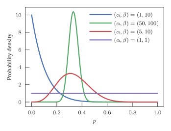
Figure 17: Beta distributions for the noise magnitudes $p$ and $q$ allow us to control the degree of prior knowledge we have on their values. For example, the values $(\alpha,\beta)=(1,10)$ represent an expectation that the value of $p$ is relatively low, with mode at $0$ and average $\alpha/(\alpha+\beta)=1/11\approx 0.09$. The values $(\alpha,\beta)=(50,100)$ express relative certainty that the value of $p$ is close to $1/3$, whereas the values $(\alpha,\beta)=(5,10)$ represent the same average expectation, but with less certainty. The values $(\alpha,\beta)=(1,1)$ express the largest amount of uncertainty about the parameter $p$, in which case it is uniformly distributed in unit interval.

In Fig. 17 are shown examples of the Beta distribution of Eq. 18, for different choices of the hyperparameters $\alpha$ and $\beta$, illustrating their meaning with respect to the prior knowledge assumed for the missing edge probability $p$ (and analogously for the spurious edge probability $q$, and its hyperparameters $\mu$ and $\nu$).

Appendix B Latent edge MCMC algorithm

As described in the main text, we use a Markov chain Monte Carlo (MCMC) algorithm to sample from the posterior distribution

$$P(\bm{A}|\bm{\mathcal{D}})=\frac{P(\bm{\mathcal{D}}|\bm{A})P(\bm{A})}{P(\bm{\mathcal{D}})},$$ (73)

where $\bm{A}$ is the network being inferred, and $\bm{\mathcal{D}}$ is the measurement data. Since we are using structured distributions in place of $P(\bm{A})$, consisting of nonparametric formulations of the SBM, its computation in closed form is not tractable. Instead, we sample from the joint posterior

$$P(\bm{A},\bm{b}|\bm{\mathcal{D}})=\frac{P(\bm{\mathcal{D}}|\bm{A})P(\bm{A}|\bm{b})P(\bm{b})}{P(\bm{\mathcal{D}})},$$ (74)

where $\bm{b}$ is the partition of nodes used for the SBM. If we sample from this distribution, and ignore the values of $\bm{b}$, we obtain the desired marginal $P(\bm{A}|\bm{\mathcal{D}})=\sum_{\bm{b}}P(\bm{A},\bm{b}|\bm{\mathcal{D}})$. However, we are often also interested in the partition itself, as it gives information on the large-scale network structure, so we often use this in our analyses as well.

The MCMC algorithm consists of making proposals of the kind $P(\bm{b}^{\prime}|\bm{A},\bm{b})$ and $P(\bm{A}^{\prime}|\bm{A},\bm{b})$ for the partition and network, respectively, and accepting them according to the Metropolis-Hastings probability

$$\min\left(1,\frac{P(\bm{A}^{\prime},\bm{b}^{\prime}|\bm{\mathcal{D}})P(\bm{A}|\bm{A}^{\prime},\bm{b}^{\prime})P(\bm{b}|\bm{A}^{\prime},\bm{b}^{\prime})}{P(\bm{A},\bm{b}|\bm{\mathcal{D}})P(\bm{A}^{\prime}|\bm{A},\bm{b})P(\bm{b}^{\prime}|\bm{A},\bm{b})}\right),$$ (75)

which does not require the computation of the intractable normalization constant $P(\bm{\mathcal{D}})$. In practice, at each step in the chain we make either a move proposal for $\bm{A}$ or $\bm{b}$, not both at once. For the node partition, we use the move proposals similar to the ones used in Refs. Peixoto (2014b, 2017), where for any given node $i$ in group $r$ we propose to move it to group $s$ (which can be previously unoccupied, in which case it is labelled $s=B+1$) according to

$$P(b_{i}=r\to s|\bm{A},\bm{b})=d\delta_{s,B+1}+{}\\ (1-d)(1-\delta_{s,B+1})\sum_{t=1}^{B}P(t|i)\frac{e_{ts}+\epsilon}{e_{t}+\epsilon B},$$ (76)

where $P(t|i)=\sum_{j}A_{ij}\delta_{b_{j},t}/k_{i}$ is the fraction of neighbors of $i$ that belong to group $t$, $\epsilon>0$ is a small parameter which guarantees ergodicity, and $d$ is the probability of moving to a previously unoccupied group. (If $k_{i}=0$, we assume $P(b_{i}=r\to s|\bm{A},\bm{b})=d\delta_{s,B+1}+(1-d)(1-\delta_{s,B+1})/B$.) This move proposal attempts to the use the currently known large-scale structure of the network to better inform the possible moves of the node, without biasing with respect to group assortativity. The parameters $d$ and $\epsilon$ do not affect the correctness of the algorithm, only the mixing time, which is typically not very sensitive, provided they are chosen within a reasonable range (we used $d=0.01$ and $\epsilon=1$ throughout). When using the HDC-SBM, we used the variation of the above for hierarchical partitions described in Ref. Peixoto (2017). The move proposals above require only minimal bookkeeping of the number edges incident on each group, and can be made in time $O(k_{i})$, which is also the time required to compute the ratio in Eq. 75, independent on how many groups are currently occupied.

For the network move proposals we could have used simple edge/nonedge flips with

$$P(A_{ij}^{\prime}=A_{ij}+\delta|\bm{A})=\begin{cases}1&\text{ if }A_{ij}+\delta=1-A_{ij},\\ 0&\text{ otherwise},\end{cases}$$ (77)

with $\delta\in\{-1,1\}$. But in fact, since we operate with latent multigraphs, the moves are slightly different, as described in Appendix D. The correctness of the algorithm does not depend on the order or the frequency with which we attempt to update the entries $(i,j)$, provided they are all eventually updated, so in principle we could choose them randomly each time. However, we have found this leads to poor mixing times, since most entries correspond to nonedges $A_{ij}=0$ which tend to remain in that state. Instead, we choose the entries to update with a probability given by the current SBM,

$$P(i,j|\bm{A},\bm{b})=\kappa_{i}\kappa_{j}m_{b_{i},b_{j}},$$ (78)

with

$$\kappa_{i}=\frac{k_{i}+1}{\sum_{j}\delta_{b_{j},b_{i}}k_{j}+1}$$ (79)

being the probability of selecting node $i$ from its group $b_{j}$, proportional to its current degree plus one, and

$$m_{rs}=\frac{e_{rs}+1}{\sum_{tu}e_{rs}+1}$$ (80)

is the probability of selecting groups $(r,s)$, where $e_{rs}=\sum_{ij}A_{ij}\delta_{b_{i},r}\delta_{b_{j},s}$. The above probabilities guarantee that every entry will be eventually sampled, but it tends to probe denser regions more frequently, which we found to typically lead to faster mixing times. This sampling can be done in time $O(1)$, simply by keeping urns of vertices and edges according to the group memberships. The time required to compute the ratio in Eq. 75 is also $O(1)$ for the DC-SBM and $O(L)$ for the HDC-SBM, where $L$ is the hierarchy depth, again independent of the number of occupied groups.

When combining both move proposals above for the partition and network, the time required to perform $V$ node proposals and $M$ edge proposals is $O({\left<k\right>}V+M)$, where ${\left<k\right>}$ is the average degree, which allows for the inference of very large networks, with up to millions of edges. A reference implementation of the above algorithm is freely available as part of the graph-tool library Peixoto (2014c).

Appendix C Nonparametric SBM formulation

Here we give a summary of the nonparametric SBMs used in this work, which are derived in detail in Ref. Peixoto (2017). We begin with the Poisson DC-SBM likelihood Karrer and Newman (2011),

$$P(\bm{A}|\bm{\lambda},\bm{\theta},\bm{b})=\prod_{i<j}\frac{e^{-\theta_{i}\theta_{j}\lambda_{b_{i},b_{j}}}(\theta_{i}\theta_{j}\lambda_{b_{i},b_{j}})^{A_{ij}}}{A_{ij}!}\times\\ \prod_{i}\frac{e^{-\theta_{i}^{2}\lambda_{b_{i},b_{i}}/2}(\theta_{i}^{2}\lambda_{b_{i},b_{i}}/2)^{A_{ii}/2}}{(A_{ii}/2)!},$$ (81)

which generates multigraphs with $A_{ij}\in\mathbb{N}$, and with self-loops allowed. By choosing the arbitrary parametrization $\sum_{i}\theta_{i}\delta_{b_{i},r}=1$ for every group $r$, $\lambda_{rs}$ becomes the expected number of edges between groups $r$ ans $s$, and $\theta_{i}$ is proportional to the expected degree of node $i$, $\theta_{i}={\left<k_{i}\right>}/\sum_{s}\lambda_{b_{i},s}$. We use the noninformative prior for $\bm{\theta}$,

$$P(\bm{\theta}|\bm{b})=\prod_{r}(n_{r}-1)!\delta({\textstyle\sum_{i}\theta_{i}\delta_{b_{i},r}-1}).$$ (82)

and $\bm{\lambda}$,

$$P(\bm{\lambda}|\bm{b})=\prod_{r\leq s}e^{-\lambda_{rs}/(1+\delta_{rs})\bar{\lambda}}/(1+\delta_{rs})\bar{\lambda}$$ (83)

with $\bar{\lambda}=2E/B(B+1)$, which results in the integrated marginal probability,

$$P(\bm{A}|\bm{b}) =\int P(\bm{A}|\bm{\lambda},\bm{\theta},\bm{b})P(\bm{\lambda}|\bm{b})P(\bm{\theta}|\bm{b})\;\mathrm{d}\bm{\lambda}\mathrm{d}\bm{\theta}$$

$$=\frac{\bar{\lambda}^{E}}{(\bar{\lambda}+1)^{E+B(B+1)/2}}\times\frac{\prod_{r<s}e_{rs}!\prod_{r}e_{rr}!!}{\prod_{i<j}A_{ij}!\prod_{i}A_{ii}!!}\times$$ (84)

$$\qquad\prod_{r}\frac{(n_{r}-1)!}{(e_{r}+n_{r}-1)!}\times\prod_{i}k_{i}!,$$ (85)

where $k_{i}=\sum_{j}A_{ij}$ is the degree of node $i$. As shown in Ref. Peixoto (2017), the above is equivalent to a microcanonical model given by

$$P(\bm{A}|\bm{b})=P(\bm{A}|\bm{k},\bm{e},\bm{b})P(\bm{k}|\bm{e},\bm{b})P(\bm{e}|\bm{b}),$$ (86)

with

$$P(\bm{A}|\bm{k},\bm{e},\bm{b}) =\frac{\prod_{r<s}e_{rs}!\prod_{r}e_{rr}!!\prod_{i}k_{i}!}{\prod_{i<j}A_{ij}!\prod_{i}A_{ii}!!\prod_{r}e_{r}!!},$$ (87)

$$P(\bm{k}|\bm{e},\bm{b}) =\prod_{r}\left(\kern-3.00003pt\left(\genfrac{}{}{0.0pt}{}{n_{r}}{e_{r}}\right)\kern-3.00003pt\right)^{-1},$$ (88)

$$P(\bm{e}|\bm{b}) =\bar{\lambda}^{E}/(\bar{\lambda}+1)^{E+B(B+1)/2},$$ (89)

being the corresponding noninformative priors. Following Ref. Peixoto (2017), we replace the microcanonical prior for the degrees with

$$P(\bm{k}|\bm{e},\bm{b})=P(\bm{k}|\bm{\eta})P(\bm{\eta}|\bm{e},\bm{b})$$ (90)

where $\bm{\eta}=\{\eta_{k}^{r}\}$ are the degree frequencies of each group, with $\eta_{k}^{r}$ being the number of nodes with degree $k$ that belong to group $r$, and

$$P(\bm{k}|\bm{\eta})=\prod_{r}\frac{\prod_{k}\eta_{k}^{r}!}{n_{r}!}$$ (91)

is a uniform distribution of degree sequences constrained by the overall degree counts, and finally

$$P(\bm{\eta}|\bm{e},\bm{b})=\prod_{r}q(e_{r},n_{r})^{-1}$$ (92)

is the distribution of the overall degree counts. The quantity $q(m,n)$ is the number of different degree counts with the sum of degrees being exactly $m$ and that have at most $n$ non-zero counts, given by

$$q(m,n)=q(m,n-1)+q(m-n,n).$$ (93)

For the node partition we use the prior,

$$P(\bm{b})=P(\bm{b}|\bm{n})P(\bm{n}|B)P(B)=\frac{\prod_{r}n_{r}!}{N!}{N-1\choose B-1}^{-1}N^{-1}.$$ (94)

which is agnostic to group sizes.

The hierarchical degree-corrected SBM (HDC-SBM) is obtained by replacing the uniform prior for $P(\bm{e}|\bm{b})$ by a nested sequence of SBMs, where the edge counts in level $l$ are generated by a SBM at a level above,

$$P(\bm{e}_{l}|\bm{e}_{l+1},\bm{b}_{l})=\prod_{r<s}\left(\kern-3.00003pt\left(\genfrac{}{}{0.0pt}{}{n_{r}^{l}n^{l}_{s}}{e_{rs}^{l+1}}\right)\kern-3.00003pt\right)^{-1}\prod_{r}\left(\kern-3.00003pt\left(\genfrac{}{}{0.0pt}{}{n_{r}^{l}(n_{r}^{l}+1)/2}{e_{rr}^{l+1}/2}\right)\kern-3.00003pt\right)^{-1},$$ (95)

where $\left(\kern-3.00003pt\left(\genfrac{}{}{0.0pt}{}{n}{m}\right)\kern-3.00003pt\right)={n+m-1\choose m}$ is the multiset coefficient. The prior for the hierarchical partition is obtained using Eq. 94 at every level. We refer to Ref. Peixoto (2017) for further details.

Directed variations of the model above are straightforward Peixoto (2017), together with their noise models considered in the text, which simply require sums and products to go over all directed node pairs. We omit the expressions here for brevity, but we used the directed models whenever appropriate.

The hierarchical model above is constructed to be agnostic about several large-scale aspects of the network, including the degree distribution, the distribution of group sizes and the mixing patterns. Due to its nonparametric nature, it can be used to infer the dimensions of the model, including the number of groups and hierarchy shape. The HDC-SBM has the additional advantage that it can detect small but statistically significant groups in large networks, where the maximum number of detectable groups scales with $O(N/\ln N)$, as opposed to the $O(\sqrt{N})$ obtainable with non-hierarchical models Peixoto (2013, 2014a).

Appendix D Adapting multigraph models to simple graphs

The SBM variations considered in the previous section generate multigraphs with self-loops, however the noise models considered in this work operate on simple graphs. The usual justification for the use of multigraph models on simple graph data is that in the sparse case they are approximately the same, since the probability of multiple edges and self-loops being generated is very small. Although this is true for uniform SBMs, like the planted partition model considered in Sec. II.3.4, it may not be true for the DC-SBM when the degree distribution is sufficiently broad. In this situation, the simple and multigraph ensembles are no longer equivalent Park and Newman (2003); Johnson et al. (2010); Garlaschelli et al. (2017), and the use of the multigraph model in this case may lead to biases. Unfortunately, the simple graph formulations of the DC-SBM cannot have their integrated likelihoods computed in closed form.

Here we adapt the multigraph models to simple graphs in tractable and simple way by generating multigraphs and then collapsing the multiple edges. In other words, if $\bm{G}$ is a multigraph with entries $G_{ij}\in\mathbb{N}$, the collapsed simple graph $\bm{A}(\bm{G})$ has binary entries

$$A_{ij}(G_{ij})=\begin{cases}1&\text{ if }G_{ij}>0\text{ and }i\neq j,\\ 0&\text{ otherwise.}\end{cases}$$ (96)

Therefore, if $\bm{G}$ is a multigraph generated by $P(\bm{G}|\theta)$, where $\theta$ are arbitrary parameters, then the corresponding collapsed simple graph $\bm{A}$ is generated by

$$P(\bm{A}|\theta) =\sum_{\bm{G}}P(\bm{A},\bm{G}|\theta),$$ (97)

$$=\sum_{\bm{G}}P(\bm{A}|\bm{G})P(\bm{G}|\theta),$$ (98)

with

$$P(\bm{A}|\bm{G})=\begin{cases}1&\text{ if }\bm{A}=\bm{A}(\bm{G}),\\ 0&\text{ otherwise.}\end{cases}$$ (99)

Even if $P(\bm{A}|\theta)$ cannot be computed in closed form, the joint distribution $P(\bm{A},\bm{G}|\theta)=P(\bm{A}|\bm{G})P(\bm{G}|\theta)$ is trivial, provided we have $P(\bm{G}|\theta)$ in closed form. Therefore, instead of directly sampling from the posterior distribution

$$P(\bm{A},\bm{b}|\bm{\mathcal{D}})=\frac{P(\bm{\mathcal{D}}|\bm{A})P(\bm{A},\bm{b})}{P(\bm{\mathcal{D}})},$$ (100)

we sample from the joint posterior

$$P(\bm{A},\bm{G},\bm{b}|\bm{\mathcal{D}})=\frac{P(\bm{\mathcal{D}}|\bm{A})P(\bm{A}|\bm{G})P(\bm{G},\bm{b})}{P(\bm{\mathcal{D}})},$$ (101)

using MCMC, treating the values $G_{ij}$ as latent variables, and then we marginalize

$$P(\bm{A},\bm{b}|\bm{\mathcal{D}})=\sum_{\bm{G}}P(\bm{A},\bm{G},\bm{b}|\bm{\mathcal{D}}),$$ (102)

which is done simply by sampling from $P(\bm{A},\bm{G},\bm{b}|\bm{\mathcal{D}})$ and ignoring the actual magnitudes of the $G_{ij}$ values, and the diagonal entries. This yields an almost identical MCMC algorithm to the one described in Appendix B, with the only difference that we keep track of the values of $G_{ij}$, which are no longer binary, but automatically give us $A_{ij}$ [which are used for the computation of $P(\bm{\mathcal{D}}|\bm{A})$]. The move proposals of the entries of $G_{ij}$ are done by unity changes,

$$P(G_{ij}^{\prime}=G_{ij}+\delta|\bm{G})=\begin{cases}1/2&\text{ if }G_{ij}>0,\\ 1&\text{ if }G_{ij}=0\text{ and }\delta=1,\\ 0&\text{ otherwise},\end{cases}$$ (103)

again for $\delta\in\{-1,1\}$.

In the case of the DC-SBM, the degree correction happens for the multigraph $\bm{G}$, and only indirectly for $\bm{A}$. But since our model is nonparametric, and the degrees of $\bm{G}$ are also generated from their own priors, this gives us a perfectly valid and useful degree-corrected model for $\bm{A}$ as well.

Appendix E Datasets

Here we give brief descriptions of the datasets used in this work, with properties listed in tables 1 and 2.

E.1 Data without primary error estimates

Karate club

Social network between $34$ members of a Karate club Zachary (1977). The version used in Table 1 is the same one used in Ref. Girvan and Newman (2002), with $A_{23,34}=1$ and hence $78$ edges in total. In Table 2, it was assumed that each repeated entry of the adjacency matrix reported in Ref. Zachary (1977) amounted to a different measurement, so that $n_{ij}=2$ and $x_{ij}=2A_{ij}$ for all $(i,j)$, except for $x_{23,34}=1$.

9/11 terrorists

Social associations between 62 terrorists responsible for the 9/11 attacks Krebs (2002a, b).

American football

Network of American football games between Division IA colleges during the regular season in fall of 2000 Girvan and Newman (2002).

Network scientists

Coauthorship network of scientists working on network science Newman (2006).

C. elegans neural

Directed neural network of the Caenorhabditis elegans worm White et al. (1986), manually compiled by Watts et al. Watts and Strogatz (1998), based on the original data. The $5$ nodes with zero degree omitted in Ref. Watts and Strogatz (1998) were included in our analysis, resulting in $N=302$ nodes in total.

Malaria genes

Bipartite gene-substring association network for malaria Larremore et al. (2013).

Power grid

Western states power grid of the United States Watts and Strogatz (1998).

Political blogs

Citations between political blogs during the 2004 presidential election in the United States Adamic and Glance (2005).

DBLP citations

Citation network of DBLP, a database of scientific publications Ley (2002).

Openflights

Directed network of flights between world-wide airports, collected from the community-driven website http://www.openflights.org.

Reactome

Network of protein–protein interactions in humans. Joshi-Tope et al. (2005)

cond-mat

Network of collaborations in papers published in the cond-mat section of the arxiv.org pre-print website in the period spanning from January 1, 1995 and March 31, 2005 Newman (2001).

Enron email

Emails sent between employees of Enron between 1999 and 2003 Klimt and Yang (2004).

Linux source

Network of Linux source code files, with directed edges denoting that they include each otherKunegis (2013).

Brightkite

Online social network from the defunct brightkite website.

PGP

Global web of trust of the Pretty-Good-Privacy (PGP) encryption protocol. Nodes are public keys, and directed edges indicate that one key digitally signed another Richters and Peixoto (2011).

Internet AS

Directed network of internet autonomous systems, ca. 2009, as measured by the Center for Applied Internet Data Analysis (CAIDA), available at https://www.caida.org/data/.

Web Stanford

Directed network of hyperlinks between the web pages from the website of the Stanford University Leskovec et al. (2008).

Flickr

Network of images in the image-sharing site http://flickr.com, where two images are connected if they share metadata, such tags, groups or location Mcauley and Leskovec (2014).

E.2 Data with primary error estimates

Reality mining

Proximity interactions between voluntary students over time Eagle and (Sandy). As measurements we considered the state of the network during eight consecutive Wednesdays in March and April of 2005.

School friends

Directed network of friendship between primary and high-school students Moody (2001). Each student have been asked repeatedly to list his or her best 5 female and 5 male friends.

Human connectome

Neuronal connections in the human brain, measured for $418$ individuals, each of which we considered as a separate measurement Szalkai et al. (2017).

References

- Barabási (2011) Albert-László Barabási, “The network takeover,” (2011).
- Marsden (1990) Peter V. Marsden, “Network Data and Measurement,” Annual Review of Sociology 16, 435–463 (1990).
- Butts (2003) Carter T. Butts, “Network inference, error, and informant (in)accuracy: a Bayesian approach,” Social Networks 25, 103–140 (2003).
- Liben-Nowell and Kleinberg (2007) David Liben-Nowell and Jon Kleinberg, “The link-prediction problem for social networks,” Journal of the American Society for Information Science and Technology 58, 1019–1031 (2007).
- Clauset et al. (2008) Aaron Clauset, Cristopher Moore, and M. E. J. Newman, “Hierarchical structure and the prediction of missing links in networks,” Nature 453, 98–101 (2008).
- Guimerà and Sales-Pardo (2009) Roger Guimerà and Marta Sales-Pardo, “Missing and spurious interactions and the reconstruction of complex networks,” Proceedings of the National Academy of Sciences 106, 22073 –22078 (2009).
- Lü and Zhou (2011) Linyuan Lü and Tao Zhou, “Link prediction in complex networks: A survey,” Physica A: Statistical Mechanics and its Applications 390, 1150–1170 (2011).
- Žnidaršič et al. (2012) Anja Žnidaršič, Anuška Ferligoj, and Patrick Doreian, “Non-response in social networks: The impact of different non-response treatments on the stability of blockmodels,” Social Networks 34, 438–450 (2012).
- Squartini and Garlaschelli (2017) Tiziano Squartini and Diego Garlaschelli, Maximum-Entropy Networks: Pattern Detection, Network Reconstruction and Graph Combinatorics (Springer, 2017).
- Newman (2018a) M. E. J. Newman, “Network reconstruction and error estimation with noisy network data,” arXiv:1803.02427 [physics] (2018a), arXiv: 1803.02427.
- Newman (2018b) M. E. J. Newman, “Network structure from rich but noisy data,” Nature Physics 14, 542–545 (2018b).
- Holland et al. (1983) Paul W. Holland, Kathryn Blackmond Laskey, and Samuel Leinhardt, “Stochastic blockmodels: First steps,” Social Networks 5, 109–137 (1983).
- Karrer and Newman (2011) Brian Karrer and M. E. J. Newman, “Stochastic blockmodels and community structure in networks,” Physical Review E 83, 016107 (2011).
- Peixoto (2017) Tiago P. Peixoto, “Nonparametric Bayesian inference of the microcanonical stochastic block model,” Physical Review E 95, 012317 (2017).
- Metropolis et al. (1953) Nicholas Metropolis, Arianna W. Rosenbluth, Marshall N. Rosenbluth, Augusta H. Teller, and Edward Teller, “Equation of State Calculations by Fast Computing Machines,” The Journal of Chemical Physics 21, 1087 (1953).
- Hastings (1970) W. K. Hastings, “Monte Carlo sampling methods using Markov chains and their applications,” Biometrika 57, 97 –109 (1970).
- Peixoto (2014a) Tiago P. Peixoto, “Hierarchical Block Structures and High-Resolution Model Selection in Large Networks,” Physical Review X 4, 011047 (2014a).
- Peixoto (2013) Tiago P. Peixoto, “Parsimonious Module Inference in Large Networks,” Physical Review Letters 110, 148701 (2013).
- Kunegis (2013) Jérôme Kunegis, “KONECT: The Koblenz Network Collection,” in Proceedings of the 22Nd International Conference on World Wide Web, WWW ’13 Companion (ACM, New York, NY, USA, 2013) pp. 1343–1350.
- Clauset et al. (2016) Aaron Clauset, Ellen Tucker, and Matthias Sainz, The Colorado index of complex networks (2016).
- Krebs (2002a) Valdis E. Krebs, “Mapping networks of terrorist cells,” Connections 24, 43–52 (2002a).
- Krebs (2002b) Valdis Krebs, “Uncloaking Terrorist Networks,” First Monday 7 (2002b), 10.5210/fm.v7i4.941.
- Zachary (1977) Wayne W. Zachary, “An Information Flow Model for Conflict and Fission in Small Groups,” Journal of Anthropological Research 33, 452–473 (1977).
- Girvan and Newman (2002) M. Girvan and M. E. J. Newman, “Community structure in social and biological networks,” Proceedings of the National Academy of Sciences 99, 7821 –7826 (2002).
- Clauset (2018) Aaron Clauset, private communication (2018).
- Havel (1955) Václav Havel, “Poznámka o existenci konečných grafů,” Časopis pro pěstování matematiky 080, 477–480 (1955).
- Hakimi (1962) S. L. Hakimi, “On realizability of a set of integers as degrees of the vertices of a linear graph. I,” J. Soc. Indust. Appl. Math. 10, 496–506 (1962).
- White et al. (1986) J. G. White, E. Southgate, J. N. Thomson, and S. Brenner, “The structure of the nervous system of the nematode Caenorhabditis elegans,” Philosophical Transactions of the Royal Society of London. Series B, Biological Sciences 314, 1–340 (1986).
- Decelle et al. (2011) Aurelien Decelle, Florent Krzakala, Cristopher Moore, and Lenka Zdeborová, “Inference and Phase Transitions in the Detection of Modules in Sparse Networks,” Physical Review Letters 107, 065701 (2011).
- Watts and Strogatz (1998) D. J. Watts and S. H. Strogatz, “Collective dynamics of ’small-world’ networks,” Nature 393, 409–10 (1998).
- Newman (2001) M. E. J. Newman, “The structure of scientific collaboration networks,” Proceedings of the National Academy of Sciences 98, 404–409 (2001).
- Eagle and (Sandy) Nathan Eagle and Alex (Sandy) Pentland, “Reality Mining: Sensing Complex Social Systems,” Personal Ubiquitous Comput. 10, 255–268 (2006).
- Szalkai et al. (2017) Balázs Szalkai, Csaba Kerepesi, Bálint Varga, and Vince Grolmusz, “Parameterizable consensus connectomes from the Human Connectome Project: the Budapest Reference Connectome Server v3.0,” Cognitive Neurodynamics 11, 113–116 (2017).
- McNab et al. (2013) Jennifer A. McNab, Brian L. Edlow, Thomas Witzel, Susie Y. Huang, Himanshu Bhat, Keith Heberlein, Thorsten Feiweier, Kecheng Liu, Boris Keil, Julien Cohen-Adad, M. Dylan Tisdall, Rebecca D. Folkerth, Hannah C. Kinney, and Lawrence L. Wald, “The Human Connectome Project and beyond: Initial applications of 300mt/m gradients,” NeuroImage Mapping the Connectome, 80, 234–245 (2013).
- Martin et al. (2016) Travis Martin, Brian Ball, and M. E. J. Newman, “Structural inference for uncertain networks,” Physical Review E 93, 012306 (2016).
- Szklarczyk et al. (2017) Damian Szklarczyk, John H. Morris, Helen Cook, Michael Kuhn, Stefan Wyder, Milan Simonovic, Alberto Santos, Nadezhda T. Doncheva, Alexander Roth, Peer Bork, Lars J. Jensen, and Christian von Mering, “The STRING database in 2017: quality-controlled protein-protein association networks, made broadly accessible,” Nucleic Acids Research 45, D362–D368 (2017).
- Strauss (1975) David J. Strauss, “A model for clustering,” Biometrika 62, 467–475 (1975).
- Hoff et al. (2002) Peter D Hoff, Adrian E Raftery, and Mark S Handcock, “Latent Space Approaches to Social Network Analysis,” Journal of the American Statistical Association 97, 1090–1098 (2002).
- Newman and Peixoto (2015) M. E. J. Newman and Tiago P. Peixoto, “Generalized Communities in Networks,” Physical Review Letters 115, 088701 (2015).
- Newman and Clauset (2016) M. E. J. Newman and Aaron Clauset, “Structure and inference in annotated networks,” Nature Communications 7, 11863 (2016).
- Hric et al. (2016) Darko Hric, Tiago P. Peixoto, and Santo Fortunato, “Network Structure, Metadata, and the Prediction of Missing Nodes and Annotations,” Physical Review X 6, 031038 (2016).
- Aicher et al. (2015) Christopher Aicher, Abigail Z. Jacobs, and Aaron Clauset, “Learning latent block structure in weighted networks,” Journal of Complex Networks 3, 221–248 (2015).
- Peixoto (2018) Tiago P. Peixoto, “Nonparametric weighted stochastic block models,” Physical Review E 97, 012306 (2018).
- Kivelä et al. (2014) Mikko Kivelä, Alex Arenas, Marc Barthelemy, James P. Gleeson, Yamir Moreno, and Mason A. Porter, “Multilayer networks,” Journal of Complex Networks 2, 203–271 (2014).
- Peixoto (2015) Tiago P. Peixoto, “Inferring the mesoscale structure of layered, edge-valued, and time-varying networks,” Physical Review E 92, 042807 (2015).
- Peixoto (2014b) Tiago P. Peixoto, “Efficient Monte Carlo and greedy heuristic for the inference of stochastic block models,” Physical Review E 89, 012804 (2014b).
- Peixoto (2014c) Tiago P. Peixoto, “The graph-tool python library,” figshare (2014c), 10.6084/m9.figshare.1164194, available at https://graph-tool.skewed.de.
- Park and Newman (2003) Juyong Park and M. E. J. Newman, “Origin of degree correlations in the Internet and other networks,” Physical Review E 68, 026112 (2003).
- Johnson et al. (2010) Samuel Johnson, Joaquín J. Torres, J. Marro, and Miguel A. Muñoz, “Entropic Origin of Disassortativity in Complex Networks,” Physical Review Letters 104, 108702 (2010).
- Garlaschelli et al. (2017) Diego Garlaschelli, Frank den Hollander, and Andrea Roccaverde, “Ensemble nonequivalence in random graphs with modular structure,” Journal of Physics A: Mathematical and Theoretical 50, 015001 (2017).
- Newman (2006) M. E. J. Newman, “Finding community structure in networks using the eigenvectors of matrices,” Physical Review E 74, 036104 (2006).
- Larremore et al. (2013) Daniel B. Larremore, Aaron Clauset, and Caroline O. Buckee, “A Network Approach to Analyzing Highly Recombinant Malaria Parasite Genes,” PLOS Comput Biol 9, e1003268 (2013).
- Adamic and Glance (2005) Lada A. Adamic and Natalie Glance, “The political blogosphere and the 2004 U.S. election: divided they blog,” in Proceedings of the 3rd international workshop on Link discovery, LinkKDD ’05 (ACM, New York, NY, USA, 2005) pp. 36–43.
- Ley (2002) Michael Ley, “The DBLP Computer Science Bibliography: Evolution, Research Issues, Perspectives,” in Proceedings of the 9th International Symposium on String Processing and Information Retrieval, SPIRE 2002 (Springer-Verlag, London, UK, UK, 2002) pp. 1–10.
- Joshi-Tope et al. (2005) G. Joshi-Tope, M. Gillespie, I. Vastrik, P. D’Eustachio, E. Schmidt, B. de Bono, B. Jassal, G. R. Gopinath, G. R. Wu, L. Matthews, S. Lewis, E. Birney, and L. Stein, “Reactome: a knowledgebase of biological pathways,” Nucleic Acids Research 33, D428–D432 (2005).
- Klimt and Yang (2004) Bryan Klimt and Yiming Yang, “Introducing the Enron Corpus.” in CEAS (2004).
- Richters and Peixoto (2011) Oliver Richters and Tiago P. Peixoto, “Trust Transitivity in Social Networks,” PLoS ONE 6, e18384 (2011).
- Leskovec et al. (2008) Jure Leskovec, Kevin J. Lang, Anirban Dasgupta, and Michael W. Mahoney, “Community Structure in Large Networks: Natural Cluster Sizes and the Absence of Large Well-Defined Clusters,” arXiv:0810.1355 (2008).
- Mcauley and Leskovec (2014) Julian Mcauley and Jure Leskovec, “Discovering Social Circles in Ego Networks,” ACM Trans. Knowl. Discov. Data 8, 4:1–4:28 (2014).
- Moody (2001) James Moody, “Peer influence groups: identifying dense clusters in large networks,” Social Networks 23, 261–283 (2001).