Exploring NSI degeneracies in long-baseline experiments

Abstract

One of the main purposes of long-baseline neutrino experiments is to unambiguously measure the CP violating phase in the neutrino sector within the three neutrino oscillation picture. In the presence of physics beyond the Standard Model, the determination of the CP phase will be more difficult, due to the already known degeneracy problem. Working in the framework of non-standard interactions (NSI), we compute the appearance probabilities in an exact analytical formulation and analyze the region of parameters where this degeneracy problem is present. We also discuss some cases where the degeneracy of the NSI parameters can be probed in long-baseline experiments.

I Introduction

Most of the Standard Model parameters in the leptonic sector have been measured with high precision, including most of the mixing angles of the PMNS matrix de Salas et al. (2017); Valencia-Globalfit (2018); Esteban et al. (2017); Capozzi et al. (2018) and the charged lepton masses Patrignani et al. (2016). It is expected that DUNEAcciarri et al. (2015); Habig (2015); Acciarri et al. (2016a, b) and Hyper-Kamiokande Abe et al. (2011, 2015) will accurately measure the CP violating phase, $\delta$, if we restrict to the standard three neutrino oscillation picture. The measurement of absolute neutrino masses is another challenge, pursued by the Katrin experiment Angrik et al. (2005).

On the other hand, the non-zero neutrino masses have motivated their theoretical explanation through beyond the Standard Model physics. One of the best motivated schemes is that of the seesaw Schechter and Valle (1980); Mohapatra and Senjanovic (1981); Gell-Mann et al. (1979); Minkowski (1977), although there are plenty of beyond the Standard Model theories searching to explain the neutrino mass pattern Valle and Romao (2015). The presence of new physics leads naturally to a degeneracy on the neutrino CP phases; for instance, non-unitarity of the leptonic mixing matrix Escrihuela et al. (2015, 2017); Fong et al. (2017); Tang et al. (2017) will lead to an ambiguity in the measurement of the standard CP violating phase, $\delta$, as has been already pointed out in Miranda et al. (2016). Models beyond the Standard Model also include the sterile neutrino hypothesis, that has also been studied in the context of long-baseline neutrino experiments Chatterjee et al. (2017); Dutta et al. (2016); Choubey et al. (2018, 2017); Blennow et al. (2017).

A model independent framework aiming to incorporate a wide set of models is the so called non-standard interaction (NSI) picture Farzan and Tortola (2018); Miranda and Nunokawa (2015); Ohlsson (2013), where the information on new physics is encoded in parameters proportional to the Fermi constant. Besides the search for new physics signals in neutrino experiments, the robustness of the standard solution has also been jeopardized by NSI Miranda et al. (2006) showing the importance of short-baseline neutrino experiments that could help constrain these parameters. Particularly, coherent elastic neutrino nucleus scattering Akimov et al. (2017) has been helpful in obtaining this restrictions Papoulias and Kosmas (2018); Esteban et al. (2018); Denton et al. (2018); Aristizabal Sierra et al. (2018) as had been foreseen in Barranco et al. (2005).

In this context, the sensitivity to NSI in the future DUNE experiment Acciarri et al. (2015) has been extensively studied de Gouvêa and Kelly (2016a, b); Coloma (2016); Coelho et al. (2012); Deepthi et al. (2017a) in order to know the expectative constraints in the future. It has been found that, as in the non-unitary case, a degeneracy appears that could weaken the resolution in the phase, $\delta$ Forero and Huber (2016). Due to this degeneracy, the sensitivity of DUNE to the standard CP phase in presence of NSI has been under inquiry Masud and Mehta (2016); Masud et al. (2016); Ge and Smirnov (2016); Liao et al. (2017); Agarwalla et al. (2016); Das et al. (2018); Blennow et al. (2016); Falkowski et al. (2018); Deepthi et al. (2017b).

In this work we focus on the NSI framework in the context of long-baseline neutrino experiments. We introduce an analysis of the exact analytical formulas and will obtain useful information to search for the regions leading to a degeneracy of the standard CP violating phase, $\delta$, with the NSI parameters. We find the values of the flavor-changing parameters that can mimic the standard appearance probabilities, making the new phase, $\phi_{e\tau}$ indistinguishable from $\delta$. We also discuss the implications of these values in the biprobability plots, a very useful tool to exhibit the degeneracy problem. On the other hand, it is also interesting to find the regions where a restriction to the NSI parameters can be done by long-baseline neutrino experiments (LBNE). It will be evinced that biprobability plots can be used to search for these regions, although in this case expectations are more limited.

II Nonstandard interactions in matter

New physics can affect the form of the different theories that consider an extended gauge symmetry, additional number of fermion singlets or extra scalars can be parametrized by the NSI parameters Ohlsson (2013); Miranda and Nunokawa (2015); Farzan and Tortola (2018). Therefore, to study the effect of new physics in the neutrino matter potential on Earth we will consider the NSI four-point effective Lagrangian, whose coupling will be proportional to the Fermi constant. In this way the non-standard interaction Lagrangian will be given as

$$\mathcal{L}_{NSI}=-2\sqrt{2}G_{F}\sum_{f}\varepsilon^{f,P}_{\alpha\beta}\left[\bar{\nu}_{\alpha}\gamma^{\rho}L\nu_{\beta}\right]\left[\bar{f}\gamma_{\rho}Pf\right],$$ (1)

where $f$ is a fermion of the first family ($e,u,d$) and $P$ is the projector operator $P=L,R$. In this work we will compute the effect of charged leptons and neutrinos propagating in matter and, therefore, we have taken $f=e$ and $\varepsilon^{u}_{\alpha\beta}=\varepsilon^{d}_{\alpha\beta}=0$. To have an estimate of our results for the case of $\varepsilon^{u}_{\alpha\beta}$ (or $\varepsilon^{d}_{\alpha\beta}$) one can consider that the density of quarks on Earth is approximately three times that for electrons Escrihuela et al. (2009, 2011).

This new interaction has a non SM contribution to the neutrino-charged lepton scattering process. As a consequence, neutrinos propagating in matter will feel a new potential, additional to the usual charged-current MSW Wolfenstein (1978) potential. This can be introduced in the propagation Hamiltonian and the total result will be

$$\widetilde{H}=H+\frac{A}{2E}\left(\begin{array}[]{ccc}1+\varepsilon_{ee}&\varepsilon_{e\mu}&\varepsilon_{e\tau}\\ \varepsilon^{*}_{e\mu}&\varepsilon_{\mu\mu}&\varepsilon_{\mu\tau}\\ \varepsilon^{*}_{e\tau}&\varepsilon^{*}_{\mu\tau}&\epsilon_{\tau\tau}\end{array}\right),$$ (2)

where $H$ is the Hamiltonian in vacuum and the matter potential $A=2\sqrt{2}G_{F}N_{e}E$, with $N_{e}$ is the electron number density and $E$ is the neutrino energy.

Due to the NSI contribution, there are non-diagonal terms in the Hamiltonian. To study the impact of NSI interactions on long-baseline experiments, wc compute here the exact expression for the oscillation probability in matter. We briefly mention the already known standard case and introduce the corresponding NSI formulas. To make the expressions more accessible to the reader, we show the flavor changing case for $\varepsilon_{e\tau}$ and set to zero all other NSI parameters.

We will compute first the effective neutrino mass in matter. We will follow the method used originally in Zaglauer and Schwarzer (1988) using an approach that is independent of the parametrization Flores and Miranda (2016). To find the exact expressions for the effective squared masses $\bar{M}_{i}^{2}\equiv\tilde{\lambda}_{i}$ in the presence of NSI, we start with the characteristic equation for the Hamiltonian in Eq. (2):

$$\tilde{\lambda}^{3}-\alpha\tilde{\lambda}^{2}+\beta\tilde{\lambda}-\gamma=0,$$ (3)

whose real solutions are given by

$$\tilde{\lambda}_{n}=\frac{\alpha}{3}+\frac{2}{3}\sqrt{\alpha^{2}-3\beta}\cos\left[\frac{1}{3}\arccos\left(\frac{2\alpha^{3}-9\alpha\beta+27\gamma}{2\sqrt{(\alpha^{2}-3\beta)^{3}}}\right)+\frac{2(n-1)\pi}{3}\right],\quad n=1,2,3$$ (4)

that in our case take the form

$$\alpha = \Delta m^{2}_{21}+\Delta m^{2}_{31}+A,$$

$$\beta = \Delta m^{2}_{31}\Delta m^{2}_{21}+A\Delta m^{2}_{21}[1-|U_{e2}|^{2}-2\operatorname{Re}(\varepsilon_{e\tau}U^{*}_{e2}U_{\tau 2})]$$ (5)

$$+ A\Delta m^{2}_{31}[1-|U_{e3}|^{2}-2\operatorname{Re}(\varepsilon_{e\tau}U^{*}_{e3}U_{\tau 3})]-A^{2}|\varepsilon_{e\tau}|^{2},$$

$$\gamma = A\Delta m^{2}_{21}\Delta m^{2}_{31}[|U_{e1}|^{2}+2\operatorname{Re}(\varepsilon_{e\tau}U^{*}_{e1}U_{\tau 1})]$$

$$- A^{2}|\varepsilon_{e\tau}|^{2}(\Delta m^{2}_{21}|U_{\mu 2}|^{2}+\Delta m^{2}_{31}|U_{\mu 3}|^{2}).$$

In this equation, the NSI parameters introduce a new dependence on the phases $\delta$ and $\varphi_{e\tau}$. This can be noticed, for instance, by looking at the terms that go as $2\operatorname{Re}(\varepsilon_{e\tau}U^{*}_{ei}U_{\tau i})$, that depend on the new phase, $\varphi_{e\tau}$. The last quadratic term, $|\varepsilon_{e\tau}|^{2}$, also introduces a new dependence on $\cos\delta$ through $|U_{\mu 2}|^{2}$.

The previous relations in Eq. (4) lead to three eigenvalue equations corresponding to the effective squared masses

$$\tilde{\lambda}_{1} = \frac{\alpha}{3}-\frac{1}{3}\sqrt{\alpha^{2}-3\beta}\eta-\frac{\sqrt{3}}{3}\sqrt{\alpha^{2}-3\beta}\sqrt{1-\eta^{2}},$$

$$\tilde{\lambda}_{2} = \frac{\alpha}{3}-\frac{1}{3}\sqrt{\alpha^{2}-3\beta}\eta+\frac{\sqrt{3}}{3}\sqrt{\alpha^{2}-3\beta}\sqrt{1-\eta^{2}},$$ (6)

$$\tilde{\lambda}_{3} = \frac{\alpha}{3}+\frac{2}{3}\sqrt{\alpha^{2}-3\beta}\eta,$$

where we have defined

$$\eta=\cos\left[\frac{1}{3}\arccos\left(\frac{2\alpha^{3}-9\alpha\beta+27\gamma}{2\sqrt{(\alpha^{2}-3\beta)^{3}}}\right)\right].$$

Once we have computed the effective masses in the NSI picture, we proceed to compute the neutrino probabilities in terms of the mixing matrix in this new basis, $\tilde{U}$. To make this computation, we rearrange first the form of our Hamiltonian in Eq. (2). This will make the appearance probability expressions more readable. Our main motivation is that, as it has been shown, the biprobability plots have an elliptic shape when the dependence of the oscillation probability on the CP violating phase $\delta$ is considered Kimura et al. (2002). We will follow the same procedure including now the dependence on the NSI parameters.

For simplicity, in what follows we will show the analysis for only one additional NSI parameter, the flavor changing $\varepsilon_{e\tau}$ and its phase $\varphi_{e\tau}$. Writing down the Hamiltonian from Eq.(2) as

$$\widetilde{H}=H+\frac{A}{2E}\mbox{diag}(1,0,0)+\frac{A}{2E}\varepsilon,$$ (7)

we can define two relations that will be useful later

$$\widetilde{H}_{\mu e} = \frac{p}{2E},$$

$$\widetilde{H}_{\mu\tau}\widetilde{H}_{\tau e}-\widetilde{H}_{\mu e}\widetilde{H}_{\tau\tau} = \frac{q}{(2E)^{2}}+\frac{A}{2E}r,$$ (8)

where

$$\frac{p}{2E} = H_{\mu e},$$ (9)

$$\frac{q}{(2E)^{2}} = H_{\mu\tau}H_{\tau e}-H_{\mu e}H_{\tau\tau},$$ (10)

$$r = H_{\mu\tau}\varepsilon^{*}_{e\tau}.$$ (11)

Note that these expressions have a similar form to the standard case Kimura et al. (2002), except for the additional dependence on $r$.

Both the vacuum Hamiltonian, $H$, and the modified matter one, $\widetilde{H}$, have the simple form

$$H=\frac{1}{2E}UMU^{\dagger},\quad\widetilde{H}=\frac{1}{2E}\tilde{U}\tilde{M}\tilde{U}^{\dagger},$$ (12)

respectively, where $\tilde{U}$ is the modified matter mixing matrix, $M=\mbox{diag}(m^{2}_{1},m^{2}_{2},m^{2}_{3})$, and $\tilde{M}=\mbox{diag}(\tilde{\lambda}_{1},\tilde{\lambda}_{2},\tilde{\lambda}_{3})$. Taking these two expressions and Eq.(II), one can find three relations for the product of $\tilde{U}_{\mu i}\tilde{U}_{ei}^{*}$:

$$\sum_{i}\tilde{U}_{\mu i}\tilde{U}^{*}_{ei} = \sum_{i}U_{\mu i}U^{*}_{ei}=0,$$ (13)

$$\sum_{i}\tilde{\lambda}_{i}\tilde{U}_{\mu i}\tilde{U}^{*}_{ei} = \sum_{i}m^{2}_{i}U_{\mu i}U^{*}_{ei}=p,$$ (14)

$$\sum_{(ijk)}^{cyclic}\tilde{\lambda}_{j}\tilde{\lambda}_{k}\tilde{U}_{\mu i}\tilde{U}^{*}_{ei} = \sum_{(ijk)}^{cyclic}m^{2}_{j}m^{2}_{k}U_{\mu i}U^{*}_{ei}+2EAr=q+2EAr.$$ (15)

From here we can see that $p$ and $q$ are functions of the usual oscillation parameters. Solving this system of equations, we found the following relation

$$\tilde{U}_{\mu i}\tilde{U}^{*}_{ei}=\frac{\tilde{\lambda}_{i}p+q+2EAr}{\tilde{\Delta}_{ji}\tilde{\Delta}_{ki}}.$$ (16)

This product of entries of $\tilde{U}$ is important because it appears in the oscillation amplitude for a muon neutrino to an electron neutrino:

$$A(\nu_{\mu}\rightarrow\nu_{e})=\sum_{i}\tilde{U}^{*}_{\mu i}\exp\left(-i\frac{\tilde{\lambda}_{i}L}{2E}\right)\tilde{U}_{ei}.$$ (17)

The oscillation probability for $\nu_{\mu}\rightarrow\nu_{e}$ is defined as the squared amplitude:

$$P(\nu_{\mu}\to\nu_{e})=|A(\nu_{\mu}\rightarrow\nu_{e})|^{2}.$$ (18)

In terms of the Jarlskog invariant $J$ defined as $J=\operatorname{Im}(J^{12}_{\mu e})$, with $J^{ij}_{\alpha\beta}=U_{\alpha i}U^{*}_{\beta i}U^{*}_{\alpha j}U_{\beta j}$ Jarlskog (1985) and the effective squared mass differences $\tilde{\Delta}_{ij}=\tilde{\lambda}_{i}-\tilde{\lambda}_{j}=\bar{M}^{2}_{i}-\bar{M}^{2}_{j}$, we have

$$P(\nu_{\mu}\to\nu_{e})=-4\sum_{(ij)}^{cyclic}\operatorname{Re}(\tilde{J}_{\mu e}^{ij})\sin^{2}\left(\frac{\tilde{\Delta}_{ij}L}{4E}\right)-2\tilde{J}\sum_{(ij)}^{cyclic}\sin\left(\frac{\tilde{\Delta}_{ij}L}{2E}\right).$$ (19)

From equation (16) we have

$$\operatorname{Re}(\tilde{J}^{ij}_{\mu e}) = \frac{\tilde{\lambda}_{i}\tilde{\lambda}_{j}|p|^{2}+|q+2EAr|^{2}+(\tilde{\lambda}_{i}+\tilde{\lambda}_{j})\operatorname{Re}[p(q^{*}+2EAr^{*})]}{\tilde{\Delta}_{ij}\tilde{\Delta}_{12}\tilde{\Delta}_{23}\tilde{\Delta}_{31}},$$ (20)

$$\tilde{J} = \frac{\operatorname{Im}[p(q^{*}+2EAr^{*})]}{\tilde{\Delta}_{12}\tilde{\Delta}_{23}\tilde{\Delta}_{31}}.$$ (21)

Let us notice that, if there were no NSI (meaning $r=0$), matter effects would only appear in the effective masses in Eq. (II) . The same would happen if we only have non-universal flavor-conserving NSI. On the other hand, the non-diagonal NSI parameters have more complex effects due to their presence in Eq. (15).

Replacing Eqs. (20) and  (21) in Eq. (19), we can find the appearance probability as a function of the CP phase $\delta$:

$$P(\nu_{\mu}\to\nu_{e})=a_{1}+a_{2}\cos\delta+a_{3}\sin\delta+a_{4}\cos 2\delta+a_{5}\sin 2\delta$$ (22)

and similarly, for anti-neutrinos oscillation $\bar{\nu}_{\mu}\rightarrow\bar{\nu}_{e}$,

$$P(\bar{\nu}_{\mu}\to\bar{\nu}_{e})=\bar{a}_{1}+\bar{a}_{2}\cos\delta+\bar{a}_{3}\sin\delta+\bar{a}_{4}\cos 2\delta+\bar{a}_{5}\sin 2\delta$$ (23)

with the coefficients $a_{k}$ defined as

$$a_{k}=\frac{-2}{\tilde{\Delta}_{12}\tilde{\Delta}_{23}\tilde{\Delta}_{31}}\sum_{(ij)}^{cyclic}\left[\frac{2w^{ij}_{k}}{\tilde{\Delta}_{ij}}\sin^{2}\left(\frac{\tilde{\Delta}_{ij}L}{4E}\right)+y_{k}\sin\left(\frac{\tilde{\Delta}_{ij}L}{2E}\right)\right],$$ (24)

where $w^{ij}_{k}$ depends on all the standard oscillation parameters and also on $\varepsilon_{e\tau}$ and $\varphi_{e\tau}$, while $y_{k}$ is independent from $\delta$. The coefficients for the antineutrino case, $\bar{a}_{k}$, have the same functional form, but with the changes $A\rightarrow-A$, $\delta\rightarrow-\delta$, and $\varphi_{e\tau}\rightarrow-\varphi_{e\tau}$.

Equations (22) and (23) have a similar form to the standard case. One difference is the appearance of the new coefficients $a_{4}$ and $a_{5}$, although we have verified that they are three orders of magnitude smaller than $a_{1}$, $a_{2}$, and $a_{3}$. Another difference is that all coefficients now depend on both phases. Again, we have verified that their variation is small, of the order of few percent.

With this exact formulation we will proceed, in the next chapter to compute the relevant appearance probabilities to study the NSI picture and to obtain the corresponding biprobility plots. As a cross check, we have also computed our results using the approximate expressions for long-baseline NSI probabilities that have been considered in Barger et al. (2002); Liao et al. (2016).

III NSI effects in long-baseline experiments

After the previous description of the exact appearance probabilities in the NSI framework, we can study the role of the NSI parameters in long-baseline neutrino experiments, in particular for the determination of the CP violating phase. Different works have studied the impact of NSI by comparing with the appearance data Coelho et al. (2012); Friedland and Shoemaker (2012) and have also discussed the potential degeneracy with a new CP phase, $\varphi_{e\tau}$, by analyzing either the expected survival probability in the presence of NSI or the expected number of events Forero and Huber (2016).

We start our discussion by computing the NSI regions that would be allowed by different long-baseline experiments. We consider the case of the T2K collaboration Abe et al. (2017), the NOVA experiment Adamson et al. (2017) and the future DUNE proposal that is expected to measure the CP phase with high accuracy. This is shown in Fig. (1), where we also show the combined case for the three experiments. We have made a scatter plot showing the points that would be allowed for the three experiments. We have considered as a test that the central value for the probabilities will be the one corresponding to the standard case with a value of $\delta=3\pi/2$ and we have assigned errors to the experiment’s measurements according to Table 1. In the same table we have mentioned the corresponding baseline and average energies considered for each experiment. In this scatter plot we have considered the central values for the standard oscillation parameters de Salas et al. (2017), a matter density of $\rho=2.84$ g/cm³ and a constant electron number density $N_{e}$. We show the different values of $\delta$, $\varepsilon_{e\tau}$, and $\varphi_{e\tau}$ that predict an allowed probability for the corresponding case. We can see that for any particular experiment there are different allowed points, leading to a relatively small region when we consider the combination of the three futuristic experimental results. Despite this, the degeneracy region is still considerably large. It is important to mention that a more detailed analysis, considering the neutrino spectrum for each experiment can reduce this degeneracy region, especially for the futuristic case of DUNE, where a wide-band beam neutrino flux will be used.

The utility of this scatter plot, as a tool for the understanding of the degeneracy regions, can be seen in Fig. (2) where we have considered the interesting case of the DUNE proposal as an example. As it is well known, biprobability plots can be studied to have a general idea of the NSI parameters restrictions, or its degeneracy. In this figure we show the biprobabilities for fixed values of $\delta$ and for the magnitude of the NSI parameter $\varepsilon_{e\tau}$. These values were easily read from Fig. (1) and, as expected, the corresponding ellipses always show a crossing point with the allowed region. The result is in agreement with already reported cases Forero and Huber (2016) and can be seen that many other values of $\varepsilon_{e\tau}$ were easily found by using the information from Fig. (1).

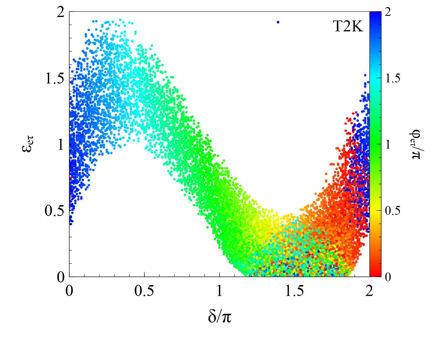
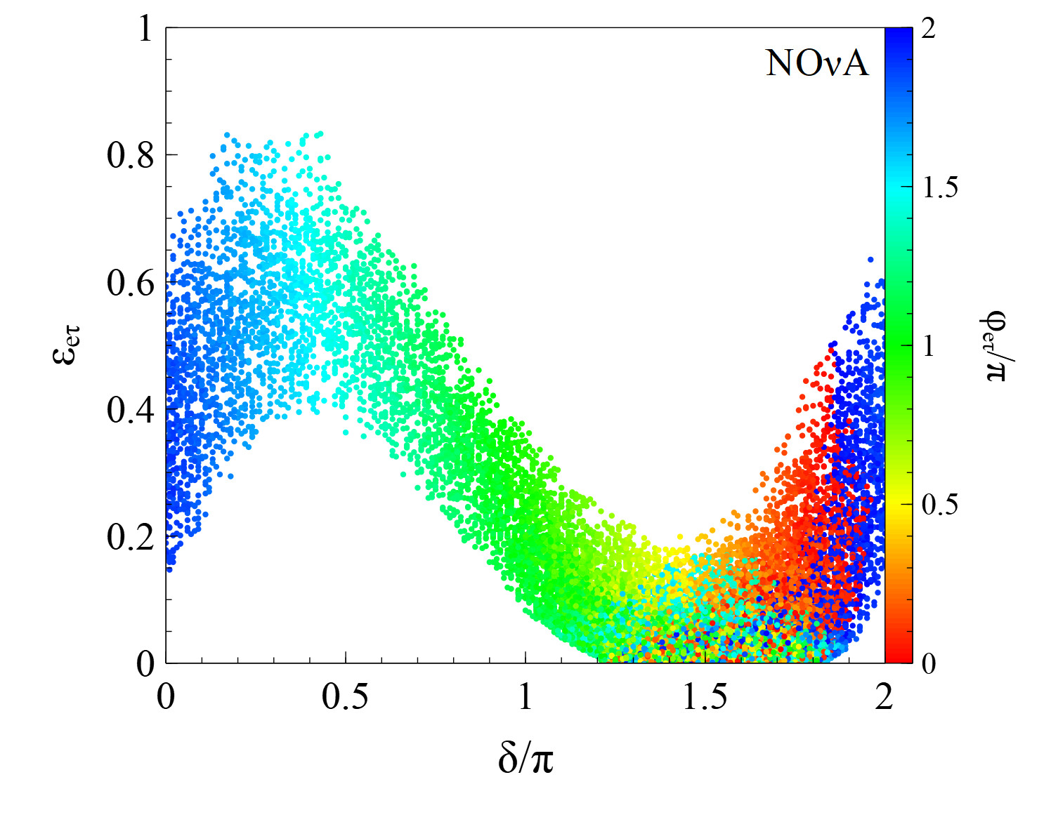
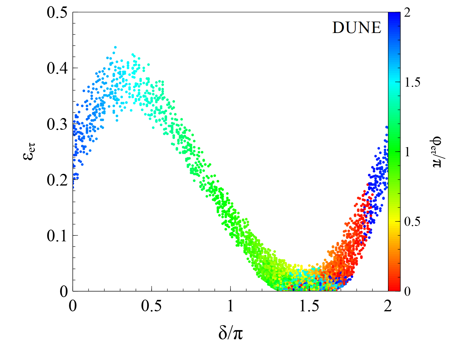
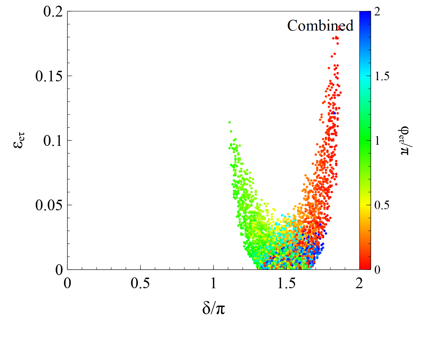
Figure 1: Scatter plot of the standard CP violating phase, $\delta$, and the non-standard parameter $\varepsilon_{e\tau}$ for a free non-standard CP phase, $\varphi_{e\tau}$. We show the dots that satisfy the biprobability region predicted by the standard oscillation picture. The first three panels show the case of T2K, NO$\nu$A and DUNE, while the bottom-right panel shows the values that satisfy simultaneously the three experiments. The uncertainties that define the appearance biprobability region, the baseline and the average energy used for these plots are shown in Table 1.

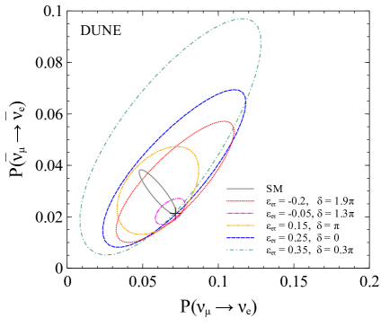
Figure 2: Biprobability plots for the DUNE proposal, varying $\varphi_{e\tau}$ from $0$ to $2\pi$, for a fixed value of the NSI magnitude of $\varepsilon_{e\tau}$ and the CP phase, $\delta$. The gray solid line represents the SM case, for varying $\delta$. Guided by the scatter plot from Fig. (1), we find ellipses that pass through the appearance biprobability region (considering a value of $\delta=3\pi/2$) marked with a cross. For the DUNE proposal we use $L=1300$ km and an average energy $E_{\nu}=3$ GeV.

	Uncertainties				Baseline (km)		Energy (GeV)
	$P(\nu_{\mu}\to\nu_{e})$		$P(\bar{\nu}_{\mu}\to\bar{\nu}_{e})$
T2K	10%		30%		295		0.6
NO$\nu$A	10%		25%		810		2.0
DUNE	5%		10%		1300		3.0

Table 1: Expected uncertainties for the neutrino and anti-neutrino appearance probability for long-baseline neutrino experiment. In the last two column the characteristic baselines and average beam energy are shown.

Another interesting analysis could be the search for restricted NSI regions, instead of a degeneracy problem, in order to look for future constraints from the DUNE experiment. We separate this discussion in two natural cases, one involving the presence flavor changing parameters, and the case of non-universal terms. For the later case, we take $\varepsilon_{ee}$ as the only parameter different from zero. As a result, according to the discussion from section II, the NSI effects will be present only in the effective masses. This implies an effective change in the potential: $V_{CC}\to V_{CC}(1+\varepsilon_{ee})$, resulting in a displaced ellipse of the same size as in the standard oscillation picture when we vary $\delta$. Several ellipses for this scenario are shown in Fig. 3, along with a curve for fixed $\delta=3\pi/2$ and a varying $\varepsilon_{ee}$. Therefore, in this case a test of the diagonal NSI parameter seems to be possible by long-baseline neutrino experiments.

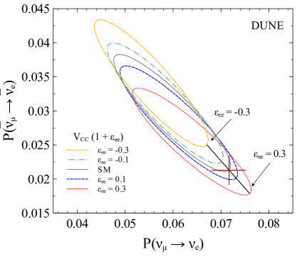
Figure 3: Biprobability plots for the DUNE proposal, considering only $\varepsilon_{ee}$ different from zero and varying $\delta$ from $0$ to $2\pi$. We show four ellipses, each for a different value of $\varepsilon_{ee}$, along with the SM case (solid gray line). The appearance probability region for DUNE is marked with a cross, considering a value of $\delta=3\pi/2$. We consider again $L=1300$ km and an average energy $E_{\nu}=3$ GeV. The presence of this diagonal NSI term only affects the standard charged-current potential as a small correction displacing the ellipse.

On the other hand, for the case non-diagonal NSI parameters, we show in Fig. (4) the biprobability curves for $\varepsilon_{e\tau}$ different from zero, varying the value of $\delta$. Since $\varepsilon_{e\tau}$ is a non-diagonal term, a new CP violating phase $\varphi_{e\tau}$ might appear. For this reason, we present two cases: $\varphi_{e\tau}=0$ in the left panel and $\varphi_{e\tau}=3\pi/2$ in the right one. As explained in the previous section, flavor-changing NSI modifies in a more complex way the oscillation probabilities and, consequently the size and orientation of the biprobability ellipses change notoriously, as seen in Fig. (4).

We can notice here that the situation is more complicated than for the diagonal NSI, making the restriction of the NSI parameters a more complicated task. For instance, for the case of a $\varphi_{e\tau}=0$, despite the particular value of $\delta=3\pi/2$ is shifted to a region different from the Standard Model prediction, a different value in the same ellipses can reach this region, allowing for a confusion for a given value of $\varepsilon_{e\tau}$. As expected, the quantitative values of $\varepsilon_{e\tau}$ and $\delta$ can be traced in the scatter plot shown in Fig. (1). For the case of $\varphi_{e\tau}=3\pi/2$, it is possible to see that the perspectives for a NSI restriction in this particular value are very promising as there are almost no crossing points of the NSI ellipses with the biprobability region, except for the particular case of a large NSI effect around $\varepsilon_{e\tau}=0.4$.

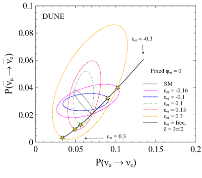
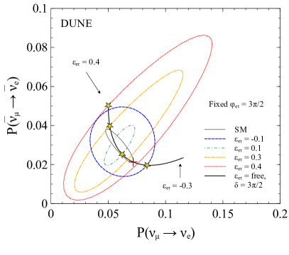
Figure 4: Biprobability plots for the DUNE proposal, varying $\delta$ from $0$ to $2\pi$, for particular values of $\varepsilon_{e\tau}$ and for $\varphi_{e\tau}=0\,(3\pi/2)$ for the left (right) panel. The gray solid line stands for the SM case, and its prediction at $\delta=3\pi/2$ is shown with a cross, including its uncertainties, which are displayed in Table 1. In both panels we can see that different values of $\varepsilon_{e\tau}$ change the orientation and size of the ellipse. The black line corresponds to a fixed value of $\delta=3\pi/2$ and $\varphi_{e\tau}=0\,(3\pi/2)$, while varying $\varepsilon_{e\tau}$ in the range $[-0.3,0.3]$, ($[-0.3,0.4]$) . In this black curve the yellow stars show its intersection with the ellipses.

IV Conclusions

In the standard three-neutrino oscillation picture, long-baseline neutrino experiments will measure the mixing parameters with precision and accuracy. In the presence of new physics the robustness of such measurements is not guaranteed and different degeneracies may appear, such as the well known LMA-D solution Miranda et al. (2006).

For the determination of the CP phase, a similar problem has been pointed out Forero and Huber (2016) when considering the flavor-changing NSI parameter $\epsilon_{e\tau}$. In this case, again, the non-oscillatory experiments will be of great help. In this work, we have focused in the interplay of different long-baseline experiments. We have shown the parameter space that will lead to an indetermination of the $\delta$ value, as well as the role of a combined restriction from several experiments. In all our computations, we have used an exact formulation, discussing its main characteristics.

The combination of different baselines can indeed help reduce the degeneracy problem, although a more detailed study is needed. Besides, we have computed the biprobability plots in the context of NSI and prove its usefulness to understand the degeneracy problem in the determination of the CP violating phase, when new physics is present. We have illustrated this with the case of the future experiment, DUNE. Although the combination of different baselines, and the wide-band beam for the DUNE neutrino flux, could help in the robust determination of the CP violating phase, short distance non-oscillatory experiments seem necessary to better constrain the NSI parameters.