Searching for a Single Community in a Graph

Abstract

In standard graph clustering/community detection, one is interested in partitioning the graph into more densely connected subsets of nodes. In contrast, the search problem of this paper aims to only find the nodes in a single such community, the target, out of the many communities that may exist. To do so , we are given suitable side information about the target; for example, a very small number of nodes from the target are labeled as such.

We consider a general yet simple notion of side information: all nodes are assumed to have random weights, with nodes in the target having higher weights on average. Given these weights and the graph, we develop a variant of the method of moments that identifies nodes in the target more reliably, and with lower computation, than generic community detection methods that do not use side information and partition the entire graph. Our empirical results show significant gains in runtime, and also gains in accuracy over other graph clustering algorithms.

1 Introduction

Community detection, or graph clustering, is the classic problem of finding subsets of nodes such that each subset has higher connectivity within itself, as compared to the average connectivity of the graph as a whole. Typically, when graphs represent similarity or affinity relationships between nodes, these subsets represent communities of similar nodes. Also typically, this problem has primarily been considered in the unsupervised setting, where the only input is the graph itself and the objective is to partition all or most of the nodes.

In this paper we look at a different, but related, community detection task, which we will refer to as the search problem. Our objective is to use the graph to find a single community of nodes – which we will call the target community – for which we have been given some relevant but quite noisy side information. We would like to do so more reliably, and with lower computation, than existing methods that do not use side information.

Our motivations are two-fold: (i) it is often the case that the network analyst is looking for nodes with a-priori specified characteristics, and (ii) it is rare that we are faced with a “pure” graph analysis problem; typically there is extra non-graphical side information that, if used properly, could make the inference task easier.

As an example setting, consider the case where we have some nodes from the target community explicitly marked as such, and our task is to recover the remaining nodes. This is a situation that frequently arises in military/intelligence settings, and also in analysis of regular consumer social networks, internet/web graphs etc. In military intelligence it can be useful to recover a single community which a known suspect is part of. Besides explicit node labels, side information could also come from meta-information one may have about the nodes; e.g. from text analysis if the graph is a web graph, or from browse/activity history of users in a social network. In recommendation system or targeted advertising it is useful to learn a community of users with a specific interest (e.g. sports) using the knowledge of how users interact with relevant contents (e.g. sports news and images). Our aim is to find a principled way to use such side information and the graph itself.

Our contributions are as follows.

• We develop a simple yet generic framework for how side information is to be specified: each node is given a (possibly random) weight, with nodes in the target community having higher weight on average than nodes not in the target – we call these biased weights. This setting would thus split an overall data + graph analysis objective into two: the analyst needs to devise a (application-dependent) procedure to convert her side information into biased node weights; these are then used by our algorithm.

• Given such biased weights, we develop a new spectral-like algorithm – specifically, a variant of the $2^{nd}$ order method of moments – to find the nodes in the target community. We call this Community Search below. In the following, we first provide the basic intuition behind it by considering the case where we have access to the population statistics of a graph coming from a stochastic block model, and then formally describe the algorithm.

• Our main results characterize the effectiveness of this algorithm in finding the target community; we study this in the standard stochastic block model setting with many communities. Analytically, we show that it matches (potentially up to log factors) the analytical guarantees of the state of the art unsupervised community detection methods; empirically, we show that the method outperforms these methods even with very noisy side information (e.g. very small number of labeled nodes), and has significantly lower computational complexity.

• We also specialize our results to the case where the side information is in the form of a small number of labeled nodes; for this case we show how one can effectively convert this to node weights, even for sparse graphs. Our experiments on a real world network further corroborate the practical applicability of this method.

1.1 Related work

While no other work has considered the problem of searching a single community in a graph, there has been a lot of research in three closely related fields; that of unsupervised and semi-supervised graph clustering, method of moments, and learning with side information. Each of these threads have a rich history – here we cover the ones most relevant to this paper.

Unsupervised graph clustering: Graph clustering or community detection has been widely studied mainly in the unsupervised setting where nodes do not have any associated labels. There is a vast literature of graph clustering algorithms both in the setting where clusters are non-overlapping Fortunato [2010] and overlapping Xie et al. [2013]. The most widely studied generative model for non-overlapping clusters in a graph is the planted partition or stochastic block model Condon and Karp [2001]. Assuming this model many algorithms have been proposed which provide statistical guarantees of recovery of all hidden clusters. These algorithms can be broadly divided into three categories (i) spectral clustering McSherry [2001]; Ng et al. [2002]; Rohe et al. [2011]; Chaudhuri et al. [2012]; Amini et al. [2013]; Yun and Proutiere [2014] (ii) convex optimization Chen et al. [2012]; Ailon et al. [2013]; Abbe et al. [2016] and more recently (iii) tensor decomposition Anandkumar et al. [2013]; Huang et al. [2013].

Semi-supervised graph clustering: The graph clustering problem has also been explored in a semi-supervised settings, where some of the nodes and/or edges are explicitly labeled. Many optimization and kernel based algorithms have been proposed Zhu [2005]; Kulis et al. [2009] to solve this problem. The popular label propagation based clustering algorithms Zhou et al. [2004]; Fujiwara and Irie [2014] are also essentially semi-supervised graph clustering algorithms with labeled nodes. Another related line of work also studies the graph clustering problem where the nodes have additional node features/attributes McAuley and Leskovec [2012]; Xu et al. [2012]; Yang et al. [2013]; Zhang et al. [2016]. More recently, local graph clustering algorithms based on message passing has also been studied in the semi-supervised setting Caltagirone et al. [2016]; Mossel and Xu [2016]; Cai et al. [2016]; Kadavankandy et al. [2018].

Method of Moments: This is a classical parameter estimation technique, where the parameters to be estimated are described in terms of the moments from the true distribution. Empirical moments are now used to replace the true moments, leading to parameter estimates Bowman and Shenton [2004]. There has been much recent interest in these methods for many statistical learning problems. These include learning Gaussian mixture models Hsu and Kakade [2013]; Anandkumar et al. [2014], LDA topic models Anandkumar et al. [2012], hidden Markov models Chang [1996] etc.

Others: There is a broader machine learning literature that incorporates the availability of extra side information into existing models and algorithms. In the context of LDA topic models, side information maybe available in the form of extra response variables for each document Mcauliffe and Blei [2008], or additional text review information of products Lu and Zhai [2008]. In collaborative filtering, side information can be of the form of item or user graph Rao et al. [2015].

In this paper we consider the community search problem with side information either in the form of biased node weights or a small set of labeled nodes.

2 Settings and Algorithm

Stochastic Block Model: Consider a graph $G=(V,E)$ with $n$ nodes and $k$ non-overlapping communities that partition the vertex set as $V=\cup_{i=1}^{k}V_{i}$. Let $\alpha_{i}=|V_{i}|/n$ be the fraction of nodes in the $i$-th community. In a stochastic block model the edge set $E$ is generated as follows. Let $0<q<p<1.$ Then for any two nodes in the same community $r,s\in V_{i}$ we have $P((r,s)\in E)=p,$ and when $r,s$ are in different community then $P((r,s)\in E)=q.$ We define this as the $(n,k,p,q)$ stochastic block model.

Target community and side information: In the search problem we are interested in the recovery of one target community, in this paper, without loss of generality, consider $V_{1}$ to be this target community. We are also provided with some side information on this target community $V_{1}.$ The side information is in the form of biased node weights. Suppose for each node $j\in V$ we are given a biased weight $w_{j}>0.$ These weights are generated by a random process satisfying the condition that for any node $j\in V$ we have $E[w_{j}|j\in V_{1}]>E[w_{j}|j\in V_{i}]$ for all $i\neq 1.$

These biased weights may be computed using a set of labeled nodes from the target community $\mathcal{L}\subset V_{1}$ (see Section 3.2). These weights can also arise from other available sources of side information. For example consider a social network graph where the target community consists of users who are sports enthusiasts. Then we can observe the amount of interaction (e.g. “likes” and “shares” in Facebook) of the users with known sports related contents. Since users in a sports community are more likely to interact with such contents, these will have the above biased node weight property. The main goal is to solve this search problem faster than the time required to recover all $k$ communities, and without any loss in estimation accuracy.

2.1 Algorithm

In this section we describe our main algorithm called Community Search. Let $X$ be the adjacency matrix of the graph $G.$ Also define community membership vectors $\mu_{1},\ldots,\mu_{k}$ where $\mu_{i}\in\mathbb{R}^{n},$ as follows. Let $\mu_{j,i}$ be the $j-$th coordinate of vector $\mu_{i}.$ Then,

$$\mu_{j,i}=\left\{\begin{array}[]{ll}p&\mbox{if }j\in V_{i}\\ q&\mbox{otherwise}\end{array}\right.$$

Note that these $\mu_{i}$-s are linearly independent and the community memberships of the nodes can be obtained from these membership vectors via thresholding. The main purpose of our algorithm is to estimate the membership vector of the first community $\mu_{1}$ (which can then be used to recover nodes in $V_{1}$).

Intuition behind our method: To understand the core of our technique, let us suppose here – just for intuition – that we actually had access to the “average” adjacency matrix $E[X]$ (recall that $X$ is the actual adjacency matrix of the stochastic block model), and let $E[X_{j}]$ be the average of the $j^{th}$ column. Then it is easy to see that $E[X_{j}]=\mu_{c_{j}}$, where $c_{j}\in 1,\ldots,k$ is the community that node $j$ belongs to. This means that the following holds for the matrix $A$ defined below:

$$A~{}:=~{}\frac{1}{n}\sum_{j=1}^{n}E[X_{j}]E[X_{j}]^{T}~{}=~{}\sum_{i=1}^{k}\alpha_{i}\mu_{i}\mu_{i}^{T}$$

Similarly, let us now also suppose that we see the “average” node weights $\bar{w}_{j}=E[w_{j}]$ for every node $j$. Then, the following holds for the matrix $B$ defined below:

$$B~{}:=~{}\frac{1}{n}\sum_{j=1}^{n}\bar{w}_{j}E[X_{j}]E[X_{j}]^{T}~{}=~{}\sum_{i=1}^{k}\alpha_{i}\omega_{i}\mu_{i}\mu_{i}^{T}$$

where in the above, for each cluster $i$, we have defined $\omega_{i}$ be the averaged weights of all nodes in that cluster. By the bias condition, we have that $\omega_{1}>\omega_{i}$ for all $i\neq 1$.

Note that both the $A$ and $B$ as defined above are symmetric positive definite rank-$k$ matrices, with the column space of each spanned by the $\mu_{i}$’s. However note also that our desired vector $\mu_{1}$ may not be an eigenvector of either $A$ or $B$; indeed if the target community $V_{1}$ is small, it may be quite far from the leading eigenvector of either matrix.

The main idea is that we can still recover $\mu_{1}$ by “whitening” $B$ using $A$, a process we describe in the proto-algorithm below. The description also provides the (simple) reason why it works – in this idealized case where average $X$ and $w$ are available.

Proto-algorithm (and explanation):

1. Compute matrices $A$ and $B$ as described above,

2. Perform rank-$k$ svd of $A$ as $A=UDU^{T},$ and let $W:=UD^{-1/2}.$ Also note that,

   $$W^{T}AW~{}=~{}I_{k}~{}=~{}\sum_{i=1}^{k}\tilde{\mu}_{i}\tilde{\mu}_{i}^{T}$$

   where we define $\tilde{\mu}_{i}:=\sqrt{\alpha_{i}}W^{T}\mu_{i}$. Now, we see that the addition of $k$ terms of the type $\tilde{\mu}_{i}\tilde{\mu}_{i}^{T}$ results in $I_{k}$; this can only happen if the corresponding $\tilde{\mu}_{i}$ are orthonormal vectors in $\mathbb{R}^{k}$. The vectors $\tilde{\mu}$ are thus “whitened” versions of the original $\mu$ vectors.

3. Next we compute the following matrix.

   $$R~{}:=~{}W^{T}BW~{}=~{}\sum_{i=1}^{k}\omega_{i}\tilde{\mu}_{i}\tilde{\mu}_{i}^{T}$$

   Now, since $\tilde{\mu}_{i}$ are orthonormal, the above equation represents an eigenvalue decomposition of the $k\times k$ size matrix $R$, with eigenvectors $\tilde{\mu}_{i}$ and corresponding eigenvalues $\omega_{i}.$ Thus, $\tilde{\mu}_{1}$ – the whitened vector corresponding to the target community – is now the leading eigenvector of $R$, because $\omega_{1}>\omega_{i}$.

4. Find $\tilde{\mu}_{1}$ by setting it to be the leading eigenvector of $R$. Finally we can recover $\mu_{1}$ from $\tilde{\mu}_{1}$ in two steps. First compute $z:=UD^{1/2}\tilde{\mu}_{1}=\sqrt{\alpha_{1}}\mu_{1}.$ Next compute vector

   $$m_{1}~{}:=~{}\frac{1}{n}\sum_{j=1}^{n}E[X_{j}]~{}=~{}\sum_{i=1}^{k}\alpha_{i}\mu_{i}$$

   We can recover $\sqrt{\alpha_{1}}=\tilde{\mu}_{1}^{T}W^{T}m_{1}.$ Then simply divide the $z$ defined above by this to find $\mu_{1}.$

An issue: Although simple, it is not straight forward to convert this intuition to an algorithm because due to inter dependencies it becomes hard to estimate these $A$ and $B$ matrices. In particular note that in the actual problem we are given the adjacency matrix $X$, and a natural impulse is to approximate A using the matrix

$$\frac{1}{n}\sum_{j=1}^{n}X_{j}X_{j}^{T}$$

Unfortunately, this is a good approximation to $E[XX^{T}]$, but $E[XX^{T}]\neq E[X]E[X]^{T}$ – and we require the latter. However we can get around these dependencies by first partitioning the graph. This is outlined in Algorithm 1 below.

For any two subsets $P,Q\subset[n]$ let $X_{P,Q}$ denote the submatrix of $X$ corresponding to the rows and columns in set $P$ and $Q$ respectively. The input parameters to Algorithm 1 are the adjacency matrix $X,$ number of communities $k,$ the set of biased node weights $(w_{1},\ldots,w_{n}),$ and a threshold $\tau.$ The output is the community estimate $\hat{V}_{1}.$

Input: Adjacency matrix $X,$ $k$, biased weights $(w_{1},\ldots,w_{n}),$ threshold $\tau$

Output: $\hat{V}_{1}$

1 Partition nodes into four sets $P_{1},P_{2},P_{3},P_{4}$ at random ;

2 Compute matrices $\hat{A}_{1}=\frac{1}{\sqrt{|P_{3}|}}X_{P_{1},P_{3}},$ $\hat{A}_{2}=\frac{1}{\sqrt{|P_{3}|}}X_{P_{2},P_{3}}$ ;

3 Compute vector $\hat{m}_{1}=\frac{1}{|P_{1}|}\sum_{j\in P_{1}}X_{P_{1},j}$ ;

4 Compute matrix $\hat{B}=\frac{1}{|P_{4}|}\sum_{j\in P_{4}}w_{j}X_{P_{1},j}X_{P_{2},j}^{T}$ ;

5 $\hat{\mu}_{P_{1}},\hat{\alpha}_{1}\leftarrow$ SearchSubroutine($\hat{A}_{1},\hat{A}_{2},\hat{B},\hat{m}_{1},k$) ;

6 Compute $V_{P_{1}}=\{j\in P_{1}:\hat{\mu}_{P_{1},j}>\tau\}$ ;

7 Repeat steps 1-1 with $P_{i}$’s rotated in order to estimate $\hat{\mu}_{P_{2}},\hat{\mu}_{P_{3}},\hat{\mu}_{P_{4}}.$ Use them to compute $V_{P_{2}},V_{P_{3}},V_{P_{4}}$ as in step 1 ;

8 Return community $\hat{V}_{1}=V_{P_{1}}\cup V_{P_{2}}\cup V_{P_{3}}\cup V_{P_{4}}$;

Algorithm 1 Community Search

Input: $\hat{A}_{1},\hat{A}_{2},\hat{B},\hat{m}_{1},k$

Output: $\hat{\mu}_{1},\hat{\alpha}_{1}$

1 Compute rank $k$-svd of matrices $\hat{A}_{1},\hat{A}_{2}:$ $\hat{A}_{1}=U_{1}D_{1}V_{1}^{T},$ $\hat{A}_{2}=U_{2}D_{2}V_{2}^{T}$;

2 Compute matrices $W_{1}=U_{1}D_{1}^{-1},$ $W_{2}=U_{2}D_{2}^{-1}$;

3 Let $u_{1}$ be the largest left singular vector of $W_{1}^{T}\hat{B}W_{2}$;

4 Compute $z=U_{1}D_{1}u_{1}$;

5 Compute $a=u_{1}^{T}W_{1}^{T}\hat{m}_{1}$;

6 Return $\hat{\mu}_{1}\leftarrow z/a$ and $\hat{\alpha}_{1}\leftarrow a^{2}$;

Algorithm 2 SearchSubroutine

3 Main Result

In this section we present our main theoretical results. First we show that when the set of biased weights $(w_{1},\ldots,w_{n})$ satisfy certain mild sufficient conditions, then Algorithm 1 is guaranteed to recover the target community $V_{1}.$ Later we show how such weights can be obtained even with a set of labeled nodes from the target community.

3.1 Recovery using biased weights

When side information is available in the form of biased weights $w_{j}$ for each node $j\in V,$ these weights need to be informative about the target community $V_{1}$ so that it could be recovered. Clearly good side information will lead to a better performance of any search algorithm. We quantify this quality of information in the following set of assumption (condition (A1) and (A2)) on the biased weights. The third condition (A3) is a more fundamental condition that determines when the community structure itself is identifiable in a stochastic block model.

• (A1) Average weight bias: Under this condition the expected weight of a node in community $V_{1}$ is greater than the expected weight of a node in any other community $V_{i}.$ Precisely the weights satisfy:

  $$E[w_{j}|j\in V_{1}]>E[w_{j}|j\in V_{i}],\ \forall i\neq 1$$

  This weight bias allows us to determine that community $V_{1}$ is being searched / preferred over the remaining communities. However we only require this to hold in expectation and the actual weights themselves may vary significantly. Clearly any algorithm which only uses the weight bias to determine community membership by simple thresholding will perform very poorly.

• (A2) Weight concentration: Let $\alpha_{max}=\max_{i\in[k]}\alpha_{i}$ and $\alpha_{min}=\min_{i\in[k]}\alpha_{i}.$ Define $\sigma_{1}(R):=E[w_{j}|j\in V_{1}],$ $\sigma_{2}(R):=\max_{i\neq 1}E[w_{j}|j\in V_{i}],$ $\gamma_{2}:=\max_{i\in[k],j\in V}|w_{j}-E[w_{j}|j\in V_{i}]|,$ and $\xi(n)=o(\sqrt{\log n})$ be any slowly growing function. Then with high probability the maximum deviation of the weights are bounded as,

  $$\frac{\gamma_{2}}{(\sigma_{1}(R)-\sigma_{2}(R))}=O\left(\min\left\{\frac{\alpha_{min}^{4}(p-q)^{4}}{\alpha_{max}^{4}p^{4}\xi(n)},\frac{\alpha_{min}^{5}\sqrt{n}(p-q)^{5}}{\alpha_{max}^{4}p^{4.5}\xi(n)}-1\right\}\right)$$

  This condition dictates that the maximum variation of the weights $\gamma_{2}$ is also small compared to the difference between the largest and second largest expected weights $\sigma_{1}(R)-\sigma_{2}(R).$ Since the weights are used primarily to construct the matrix $B$ in Algorithm 1, this condition ensures that the matrix $B$ can be estimated up to a tolerable error.

• (A3) $p,q$ separation: Let $p,q,n$ satisfy

  $$\frac{(p-q)^{2}}{p\sqrt{p}}=\tilde{\Omega}\left(\frac{\alpha_{max}}{\alpha_{min}^{2}\sqrt{n}}\right)$$

  This condition fundamentally determines when communities are identifiable in a stochastic block model and similar conditions are required for other community detection algorithms Anandkumar et al. [2013]; Chaudhuri et al. [2012]; Chen et al. [2012]. The more the gap $p-q$ easier it is to identify communities. Hence this condition gives a lower bound on $p-q$ which is required for community identifiability.

Theorem 1 shows that under the above assumptions on the biased weights Algorithm 1 can reconstruct community $V_{1}$ with high accuracy.

Theorem 1.

Consider a $(n,k,p,q)$ stochastic block model satisfying condition (A3). Given biased weights $(w_{1},\ldots,w_{n})$ satisfying conditions (A1), (A2), then Algorithm 1 recovers community $V_{1}$ with fraction of error nodes $o(1)$ with high probability.

Remark 1.

For a stochastic block model with equal community sizes $n/k$ condition (A3) reduces to $\frac{(p-q)^{2}}{p\sqrt{p}}=\tilde{\Omega}\left(\frac{k}{\sqrt{n}}\right).$ When $p=\Theta(p-q)$ this has the same scaling as other community detection algorithms Chen et al. [2012]; Anandkumar et al. [2013]; Chaudhuri et al. [2012]. Therefore even in sparse graphs where $p,q=\Theta\left(\frac{\log n}{n}\right)$ or for small community sizes up to $\Omega(\sqrt{n})$ nodes Algorithm 1 can recover the community.

In Theorem 1 the $o(1)$ fraction error can be easily converted to a zero error guarantee using an additional post-processing step. Instead of estimating community $1$ nodes inside partition $P_{1}$ we can estimate those in partition $P_{2},$ first by observing for each node $j\in P_{2}$ the number of edges shared with the estimated set $V_{P_{1}},$ followed by thresholding. Since $V_{P_{1}}$ estimates $V_{1}\cap P_{1}$ up to only $o(\alpha_{1}n)$ error nodes this does not cause any errors in thresholding, with high probability. This post-processing step is also independent of the previous steps in the algorithm since the edges between partitions $P_{1}$ and $P_{2}$ are not utilized in Algorithm 1. The following theorem formalizes this idea.

Theorem 2 (Exact recovery).

In a $(n,k,p,q)$ stochastic block model, under assumptions (A1)-(A3), Algorithm 1 with an additional degree thresholding step can recover community $V_{1}$ completely with high probability.

We prove Theorems 1 and 2 in Appendix A.

3.2 Recovery using labeled nodes

Biased weights, as required in Theorem 1, can be obtained from a small set of labeled nodes $\mathcal{L}$ as follows:

• Choose a radius $r$

• Weight $w_{i}$ is the number of edges between nodes in $\mathcal{L}$ and nodes at a distance of $r$ hops from node $i$

Note that the weight can also be viewed as the number of neighbors of the set $\mathcal{L}$ which are at a distance $r$ from node $i.$ Larger choice of radius $r$ means less variance in the weights, but also potentially less bias if it becomes too large. For example, $r=1$ means only neighbors of labeled nodes get weights; this is very high bias but also high variance.

The theorem below provides the correct way to choose the radius $r$ such that the weights $w_{i}$ can be made to satisfy conditions (A1), (A2). This means that even with such weights computed via labeled nodes we can efficiently find community $V_{1}$ using Algorithm 1. Note that when $p\geq\frac{1}{\sqrt{n}}$ then with high probability the labeled nodes in $\mathcal{L}$ has neighbors with any other node $i\in V_{1}\backslash\mathcal{L},$ hence the number of common neighbors between $i$ and nodes $l\in\mathcal{L}$ can be taken as weights $w_{i}$ which will satisfy conditions (A1), (A2). However this does not work for sparse graphs when $p<\frac{1}{\sqrt{n}}.$ In the following theorem we show that even for $p=\Theta\left(\frac{\log n}{n^{\epsilon}}\right),$ $\frac{1}{2}\leq\epsilon\leq 1$ the weights chosen by the above procedure and a correct $r$ will work.

Theorem 3.

Consider a $(n,k,p,q)$ stochastic block model satisfying condition (A3) where $p=\Theta\left(\frac{\log n}{n^{\epsilon}}\right),$ $q=\Theta\left(\frac{\log n}{n^{\epsilon}}\right),$ $p-q=\Theta\left(\frac{\log n}{n^{\epsilon}}\right)$ and all equal sized communities, where $\frac{1}{2}\leq\epsilon\leq 1.$ Given $L=\tilde{\Omega}(n^{\epsilon/2})$ labeled nodes, the biased weights computed with $r=\frac{2\log(n^{\epsilon}/L)}{\log np},$ satisfy conditions (A1), (A2) with high probability.

We prove this in Appendix A.3. For simplicity in Theorem 3 we assume equal community sizes, however this can be extended to unequal but comparable community sizes.

3.3 Parallel semi-supervised graph clustering

Our algorithm naturally provides a method for the standard semi-supervised graph clustering problem. This is the setting where we are given a small number of labeled nodes from every community, and we are interested in recovering all communities. In such a scenario we can apply the community search algorithm to search for each individual community using the labeled nodes in that target community. Moreover this search can be performed in parallel. Therefore Algorithm 1 can also be used as a parallel graph clustering algorithm. Note that the vector $m_{1}$ and matrices $A_{1},A_{2}$ remain the same for individual searches, only matrix $B$ should be computed separately for every target community. Section 4 shows some numerical results evaluating the performance of Algorithm 1 in this semi-supervised graph clustering setting.

3.4 Comparison

In this section we compare the theoretical performance of our algorithm with other unsupervised graph clustering algorithms.

For graphs with equal communities of size $n/k,$ convex optimization based algorithms by Chen et al. [2012]; Ailon et al. [2013]; Agarwal et al. [2015] can achieve the performance bound $\frac{(p-q)}{\sqrt{p}}=\tilde{\Omega}\left(\frac{k}{\sqrt{n}}\right).$ In comparison our algorithm achieves a slightly higher bound $\frac{(p-q)^{2}}{p\sqrt{p}}=\tilde{\Omega}\left(\frac{k}{\sqrt{n}}\right).$ However when $p=\Theta(p-q)$ both bounds are equivalent (up to log factors) implying our algorithm can recover communities even in sparse graphs with $p,q=\Theta\left(\frac{\log n}{n}\right)$ and for growing number of communities $k=O(\sqrt{n}).$ In terms of runtime our algorithm runs in $O(n^{2}k)$ time faster than $\Omega(n^{3})$ time required by convex optimization based algorithms.

The Community Search by Whitening algorithm is also faster than tensor decomposition based graph clustering algorithm by Anandkumar et al. [2013]. Note that the first step of this tensor algorithm is to compute a whitening matrix using rank–$k$ svd, which is identical to the search algorithm. In the remaining steps, for the tensor algorithm, the bulk of the computation is a rank–$k$ tensor decomposition requiring $O(k^{5})$ computation, which is slower than rank–$1$ svd computed in $O(k^{2})$ time by the search algorithm. This is corroborated by our experiments in Section 4.

Recently a quasi–linear time graph clustering algorithm was presented by Abbe and Sandon [2015] for the case when number of communities $k=O(1)$. In comparison our algorithm can be applied even when the number of communities scale as $k=O(\sqrt{n}),$ and it requires much lesser knowledge of model parameters than the former.

4 Experiments

In this section we present our numerical results showing the performance of the Community Search algorithm on synthetic and real datasets. We compare our algorithm with the Spectral clustering algorithm by Ng et al. Ng et al. [2002] and the Tensor decomposition based clustering algorithm by Anandkumar et al. Anandkumar et al. [2013]. We generate synthetic datasets according to the stochastic block model (see Section 2) with $n=1000$ nodes, $k\in\{5,8\}$ communities, and different values of $p$ and $q.$ The real world network we consider is the US political blogosphere network first introduced in Adamic and Glance [2005]. The Spectral clustering algorithm Ng et al. [2002] requires clustering of the rows corresponding to bottom $k$ eigenvectors of the normalized Laplacian. Although k-means may be used for this, it tends to converge to local minima resulting in poor performance. To prevent this we perform clustering of the rows via the hierarchical SLINK algorithm Sibson [1973]. We refer to this Spectral+SLINK algorithm simply as Spectral clustering in the remaining section. Our algorithm implementations are all in Matlab. We consider two types of side information: labeled nodes and synthetic weights.

Labeled Nodes: As discussed earlier, this is a natural means of providing side information to the algorithm. A set of $m$ labeled nodes are randomly chosen from the target community $V_{1}.$ The corresponding weights are then computed as described in Section 3.2 with $r\in\{1,2\}.$

Synthetic Weights: We synthetically generate three sets of weights, each of which are (on average) larger over the target community. These weights are generated as follows. A pair of weights $(w_{1},w_{2})$ are first chosen to be one of $\{(5,8),(5,10),(5,12)\}.$ For each node in community $V_{1},$ we set the node’s weight to be $w_{2}$ with probability $0.8,$ and $w_{1}$ other-wise. For all other nodes in $V\backslash V_{1},$ we swap the probabilities, i.e., we set a node’s weight to be $w_{2}$ with probability $0.2$ and $w_{1}$ other-wise. This process generates three possible values of the expected node weights in the target community, $\sigma_{1}(R)\in\{7.4,9,10.6\}.$

Performance Metrics: Note that our algorithm directly uses labeled nodes/biased node weights, and the graph to infer the target community. The baseline algorithms however first estimate all communities in the graph, then it computes the average node weight in each community, finally outputs as target the community which has the highest average node weight. The estimation error for the $i$-th community is given as $e_{i}=|\{j\in V:j\in V_{i},j\not\in\hat{V}_{i}\ or\ j\in\hat{V}_{i},j\not\in V_{i}\}|.$ We compute the error for searching each community and plot either the overall average, or average over a subset of clusters. Let $T_{\mathcal{A}_{1}},T_{\mathcal{A}_{2}}$ be the runtimes of algorithms $\mathcal{A}_{1},\mathcal{A}_{2}$ respectively. Then we define speedup $s$ of algorithm $\mathcal{A}_{1}$ over algorithm $\mathcal{A}_{2}$ as $s=T_{\mathcal{A}_{2}}/T_{\mathcal{A}_{1}}.$ $s>1$ implies algorithm $\mathcal{A}_{1}$ is faster than $\mathcal{A}_{2}.$

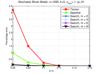
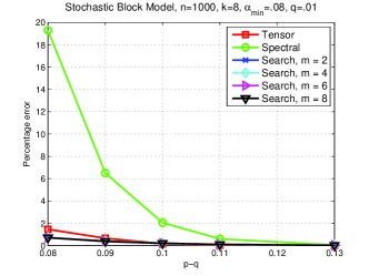
Figure 1: Labeled Nodes: Comparing the average error performance of Community Search algorithm with Spectral clustering Ng et al. [2002] and Tensor decomposition Anandkumar et al. [2013] algorithms in a stochastic block model with (a) $n=1000,$ $k=5,$ $\alpha_{min}=.1,$ (b) $n=1000,$ $k=8,$ $\alpha_{min}=.08.$ The algorithms use $m$ labeled node from target cluster as side information and compute biased weights. The Community Search algorithm outperforms both Spectral clustering and Tensor decomposition.

4.1 Performance and Speedup with Labeled Nodes

First we compare the error performance of Community Search algorithm with Spectral clustering and Tensor decomposition algorithms in the setting where side information is given in the form of $m$ labeled nodes from the target community. We then compute biased weights $w_{j}$ using the tree method of Section 3.2 with a radius $r=2.$ Note that this tree method may assign weights in violation of condition (A1) for small target communities, since for small target clusters the number of nodes in the tree from a large cluster may exceed those from the target community, in such cases Algorithm 1 cannot be expected to recover the communities. Therefore we consider a subset of larger communities which assign the correct weights satisfying condition (A1) and evaluate our algorithm over these communities. Figure 1 (a) plots the average error over $3$ largest cluster in a stochastic block model (SBM) with $n=1000,$ and $k=5$ unequal sized communities. The Community Search shows significantly less error than Tensor decomposition and Spectral clustering. In Figure 1 (b) we plot the average over $5$ larger cluster in a SBM with $n=1000,$ $k=8$ unequal communities. Again Community Search shows better error than Spectral clustering and comparable error to Tensor decomposition.

Figure 2 show the speedup performance of the Community Search and Spectral clustering algorithms over Tensor decomposition in this setting with labeled nodes. As indicated earlier, all three algorithms were implemented in Matlab. We observe that the Community Search has a much lower runtime than both Spectral clustering and Tensor decomposition.

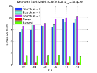
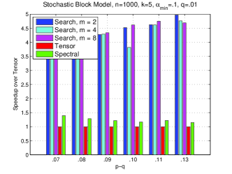
Figure 2: Labeled Nodes: The average speedup performance of the Community Search and Spectral clustering Ng et al. [2002] algorithms with respect to Tensor decomposition Anandkumar et al. [2013] in a stochastic block model with (a) $n=1000,$ $k=8,$ $\alpha_{min}=.08,$ (b) $n=1000,$ $k=5,$ $\alpha_{min}=.1,$ and labeled nodes as side information. The Community Search algorithm is faster than both Spectral clustering and Tensor decomposition.

4.2 Performance and Speedup with Synthetic Weights

Next we compare the error and runtime performance of all three algorithms in a setting where side information is available in the form of synthetically generated biased weights (as discussed earlier, three different choices of parameters). Figure 3 (a) plots the average error over all communities in a SBM with $n=1000,$ $k=8.$ The Community Search algorithm has a better performance over Spectral clustering and comparable performance with Tensor decomposition. In Figure 3 (b) plots the average error in a SBM with $n=1000,$ $k=5.$ In this case Community Search outperforms Tensor decomposition and has comparable performance to Spectral clustering.

In Figure 4 we plot the average speedup of Community Search and Spectral clustering over Tensor decomposition. Again the Community Search algorithm is significantly faster than both Spectral clustering and Tensor decomposition. We also observe that the speedup increases with increasing $p-q.$

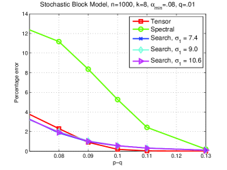
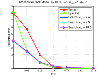
Figure 3: Synthetic Weights: Comparing the average error performance of Community Search algorithm with Spectral clustering Ng et al. [2002] and Tensor decomposition Anandkumar et al. [2013] algorithms in a stochastic block model with (a) $n=1000,$ $k=8,$ $\alpha_{min}=.08,$ (b) $n=1000,$ $k=5,$ $\alpha_{min}=.1.$ The algorithms use synthetic weights as side information to search for the target community. Community Search algorithm shows a lower error.

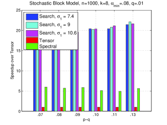
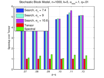
Figure 4: Synthetic Weights: The average speedup performance of the Community Search and Spectral clustering Ng et al. [2002] algorithms with respect to Tensor decomposition Anandkumar et al. [2013] in a stochastic block model with (a) $n=1000,$ $k=8,$ $\alpha_{min}=.08,$ (b) $n=1000,$ $k=5,$ $\alpha_{min}=.1,$ and synthetic weights as side information. The Community Search algorithm is faster than both Spectral clustering and Tensor decomposition.

4.3 Sensitivity

In order to determine the sensitivity of our algorithm with respect to the quality of side information, and the number of communities $k,$ we perform the following two experiments.

First, to see how the quality of side information effects the performance of our algorithm we plot the average error with increasing singular value gap $\sigma_{1}(R)-\sigma_{2}(R)$ (or the difference between the largest and second largest expected node weight) in Figure 5. In this experiment we fix the synthetic weights $(w_{1}=5,w_{2}=10)$ and vary $\sigma_{1}(R)-\sigma_{2}(R)$ by changing the probabilities with which the weights appear in each community. Note that the singular value gap increases when one weight appears with greater chance than the other. Therefore $\sigma_{1}(R)-\sigma_{2}(R)$ can also be viewed as a measure of quality of side information. As predicted from our analysis, we observe that the error improves with an increase in the gap $\sigma_{1}(R)-\sigma_{2}(R).$

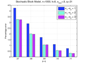
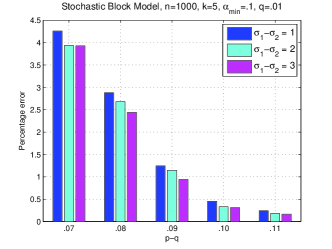
Figure 5: Sensitivity to side information: The average percentage error of Community Search Algorithm in a stochastic block model with (a) $n=1000,$ $k=8,$ $\alpha_{min}=.08,$ (b) $n=1000,$ $k=5,$ $\alpha_{min}=.1,$ with increasing singular value gap $\sigma_{1}(R)-\sigma_{2}(R).$ As shown in our analysis the performance improves with increase in the singular value gap.

Often in real applications one do not have perfect knowledge of the number of communities $k$ in a graph, which is required to run any community search or detection algorithm. Thankfully, there are several methods to estimate the parameter $k$ e.g. from the spectral properties of the graph Chen et al. [2012]; Newman and Reinert [2016]. Another approach is to compute a suitable community quality score metric like modularity Newman [2006]; Yang and Leskovec [2012] after running the algorithm with different values of $k,$ and choosing the $k$ which produce a community with the best score. However, such estimation may not be always accurate. Therefore it is crucial that any community search algorithm perform robustly with respect to the input parameter $k$ in the algorithm. In our next experiment we compare the sensitivity of our Community Search algorithm with Spectral clustering and Tensor decomposition when provided with imperfect parameter $k.$ In Figure 6 we plot the average percentage error of all three algorithms on two different SBM. We observe that even with imperfect knowledge of $k$ the Community Search algorithm has lower error than Spectral clustering and Tensor decomposition. Interestingly, the Community Search algorithm shows much less sensitivity to higher $k$ values than a lower $k$ (with respect to the ground truth $k$).

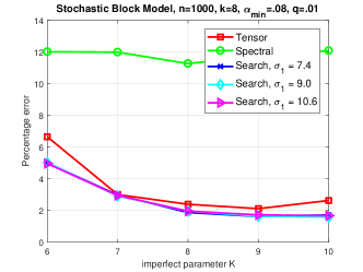
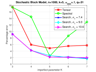
Figure 6: Sensitivity to $k$: The average percentage error of Community Search algorithm in a stochastic block model with (a) $n=1000,$ $k=8,$ $\alpha_{min}=.08,$ (b) $n=1000,$ $k=5,$ $\alpha_{min}=.1,$ $p=.09,q=.01$ in both models, synthetic weights as side information, and with imperfect knowledge of number of communities $k.$ Our Community Search algorithm exhibits lower sensitivity and error than Spectral clustering Ng et al. [2002] and Tensor decomposition Anandkumar et al. [2013] algorithms for both models.

4.4 Parallel Clustering

Finally, we consider the semi-supervised graph clustering setting described in Section 3.3 where we are provided with $m$ labeled nodes from each community, and we want to recover all communities. Recall that the Community Search algorithm can also be used as a semi-supervised parallel graph clustering algorithm. Figure 7 plots the cumulative error over all communities with increasing $p-q$ in a SBM with $n=1000,$ $k=8,$ and using different number of labeled nodes. The weights in this case are computed using the tree method and with radius $r=1.$ The Community Search algorithm outperforms both Spectral clustering and Tensor decomposition algorithms in both the experiments.

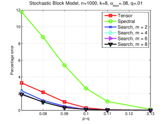
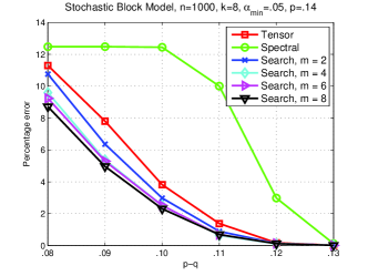
Figure 7: Labeled Nodes $+$ Parallel Clustering: Comparing the average error performance of Community Search algorithm with Spectral clustering Ng et al. [2002] and Tensor decomposition Anandkumar et al. [2013] algorithms in a stochastic block model with $n=1000,$ $k=8,$ $\alpha_{min}=.08,$ (a) $q=.01,$ (b) $p=.14.$ We consider the semi-supervised graph clustering setting when side information is available in the form of $m\in\{2,4,6,8\}$ labeled node from each community. The Community Search algorithm has a better performance over both Spectral clustering and Tensor decomposition.

4.5 Results on real dataset

In this section we evaluate the performance of Community Search algorithm on two real world networks.

In the first experiment we consider the US political blogosphere network first introduced by Adamic and Glance [2005] where nodes correspond to political blogs classified as either liberal or conservative during 2004 US election, and edges represent hyperlinks between them. We consider the largest connected component of the network having $1222$ nodes and $16,716$ edges. This dataset provides the ground-truth labels (liberal or conservative) for each node; these labels were manually generated by authors in Adamic and Glance [2005] according to their content. The largest component has two communities of sizes $586$ and $636$ according to this ground-truth.

Table 1: Average and best classification error (number of nodes that are misclassified in each estimated community compared to ground-truth) obtained by Community Search algorithm (W) with Spectral clustering (S) Ng et al. [2002] and Tensor decomposition (T) Anandkumar et al. [2013] algorithms on US political blogosphere network Adamic and Glance [2005]. The Community Search algorithm achieves the best classification error of $53$ and better average error over the competing algorithms.

	W ($m=2$)	W ($m=4$)	W ($m=6$)	W ($m=8$)	W ($m=10$)	T	S
Mean	$56$	$55.64$	$55.32$	$55.30$	$54.98$	$60$	$70$
Best	$55$	$54$	$54$	$53$	$53$	$60$	$70$

In this semi-supervised graph clustering setting, we randomly choose $m\in\{2,4,6,8,10\}$ labeled nodes from each ground-truth community as side information. Our performance metric is the classification error, namely, the number of nodes wrongly classified in each estimated community compared to the ground-truth communities ($e=|\{j\in V:j\in V_{1},j\not\in\hat{V}_{1}\ or\ j\in\hat{V}_{1},j\not\in V_{1}\}|$).

For each $m$ we observe the overall performance of the Community Search algorithm over $50$ different random choices of labeled nodes. As before, we compare the performance with Tensor decomposition and Spectral clustering algorithms. For the Community Search algorithm we compute weights using the tree method with radius $r=1.$ In Table 1, we show the best and average classification error obtained by the clustering algorithms. With $r=1$ the Community Search algorithm shows a better classification error than both Tensor and Spectral algorithms. In fact our algorithm achieves the best classification error of $53,$ which is better than other state–of–the–art algorithms Jin [2015]; Gao et al. [2017] which achieved errors in the range $58-60$ on this dataset. We also perform an in-depth analysis of the error cases in this dataset. We observed that $50$ nodes in the graph do not satisfy the community definition since they share fewer neighbors in their ground truth community (in degree) than the second community (out degree). Since the best error in our algorithm is $53,$ it appears that our algorithm performs close to the best achievable error in this dataset.

In our next experiment we consider the Facebook–ego network dataset from Leskovec and Krevl [2014], first introduced in Leskovec and Mcauley [2012]. The network corresponds to a Facebook graph with $4039$ user nodes and $88,234$ edges. The dataset also contains $193$ ground-truth ego circles, where each circle is a group of user sharing a particular interest e.g. circle of college friends, family etc. Hence each circle here corresponds to a community. We consider the $10$ largest circles with more than $100$ nodes each as the ground-truth communities. Note that in this dataset some user can belong to multiple circles/communities, unlike a typical SBM. We remove such nodes from the ground-truth communities, but not from the graph. Even after this pruning step $9$ out of $10$ ground-truth communities have more than $100$ users each. Next, we try to recover these $9$ largest ground-truth communities by randomly choosing $m\in\{5,10,15\}$ nodes as labeled nodes. We run our Community Search algorithm by computing weights using the tree method with radius $r=1,$ and we compare the average percentage estimation error (according to ground-truth) with that of Spectral clustering and Tensor decomposition algorithms. From the results presented in Table 2 we observe that the Community Search algorithm has lower average error than the baselines even with just $m=5$ labeled nodes. Also, as expected the error reduces with increasing number of labeled nodes.

Table 2: Average percentage error obtained by Community Search algorithm (W) with Spectral clustering (S) Ng et al. [2002] and Tensor decomposition (T) Anandkumar et al. [2013] algorithms to estimate $9$ largest ego circles in Facebook–ego network Leskovec and Mcauley [2012]. The Community Search algorithm achieves lower average error than the competing algorithms.

	W ($m=5$)	W ($m=10$)	W ($m=15$)	T	S
Average Error	$4.204\%$	$2.712\%$	$2.708\%$	$4.927\%$	$4.462\%$

5 Conclusion and Discussion

In this paper we defined the search problem in community detection, provided a simple generic framework for incorporating side information, and a corresponding algorithm to solve the problem. Our algorithm analytically matches the state of the art performance of existing algorithms that do not use side information, and empirically outperforms them on reliability and speed.

More generally, we believe that incorporating side information into graph analysis is a fertile and important area of research, as no real-world problem is a “pure” graph problem (i.e. where the only input is a graph) of the kind studied in e.g. the vast majority of clustering literature.

There are several possible future directions: (A) Understanding fundamental limits of community detection Mossel et al. [2014]; Montanari [2015] when there is non-trivial side information (e.g. $\Theta(\log n)$ of labeled nodes in a community). (B) Richer notions of side information, and corresponding problem definitions beyond search. (C) From a more practical viewpoint we show in our experimental results (Section 4) that even this simple form of side information can dramatically reduce the computation time for searching communities, and also improve error performance. As discussed in the previous section this work also provides a new method to parallelize graph clustering, an inherently difficult task. Adapting even faster algorithms, e.g. those based on belief-propagation, to this new semi-supervised setting is also an important prospect.

Appendix A Community Search: Proofs

In this section we provide the proof details of Theorem 1, Theorem 3 and the relevant Lemmas.

A.1 Community Search: Perturbation Analysis

Let the expectation of the estimates $\hat{m}_{1},$ $\hat{A}_{1},$ $\hat{A}_{2}$ and $\hat{B}$ be represented by $m_{1},$ $A_{1},$ $A_{2},$ $B$ respectively. Let $n_{i}=|P_{i}|$ be the size of partition $P_{i}.$ For a matrix $M,$ $\|M\|$ denotes its spectral norm. Recall that,

$$A_{1} = \frac{1}{\sqrt{n_{3}}}E[X_{P_{1},P_{3}}]\ ,\ A_{2}=\frac{1}{\sqrt{n_{3}}}E[X_{P_{2},P_{3}}]$$

$$m_{1} = \sum_{i=1}^{k}\alpha_{i}\mu_{P_{1},i}\ ,\ B=\sum_{i=1}^{k}\alpha_{i}\omega_{i}\mu_{P_{2},i}^{T}$$

where $\omega_{i}=E[w_{j}|j\in V_{i}].$ Let the rank $k$-svd of $A_{1},A_{2}$ be given by $A_{1}=U_{1}D_{1}V_{1}^{T},$ $A_{2}=U_{2}D_{2}V_{2}^{T},$ and for the estimates $\hat{A}_{1}=\hat{U}_{1}\hat{D}_{1}\hat{V}_{1}^{T},$ $\hat{A}_{2}=\hat{U}_{2}\hat{D}_{2}\hat{V}_{2}^{T}.$

Lemma 4.

Let $\max\{\|\hat{A}_{1}-A_{1}\|,\|\hat{A}_{2}-A_{2}\|\}\leq\epsilon_{2}$ and $\epsilon_{2}<\min\{\sigma_{k}(A_{1}),\sigma_{k}(A_{2})\}/12.$ Let $\hat{W}_{1}=\hat{U}_{1}\hat{D}_{1}^{-1},\hat{W}_{2}=\hat{U}_{2}\hat{D}_{2}^{-1}$ be the whitening matrices. Then,

$$\|I_{k}-(\hat{W}_{1}^{T}A_{1}A_{1}^{T}\hat{W}_{1})^{1/2}\| \leq \frac{6\epsilon_{2}}{\sigma_{k}(A_{1})}$$

$$\|I_{k}-(\hat{W}_{1}^{T}A_{1}A_{1}^{T}\hat{W}_{1})^{-1/2}\| \leq \frac{12\epsilon_{2}}{\sigma_{k}(A_{1})}$$

$$\|I_{k}-(\hat{W}_{2}^{T}A_{2}A_{2}^{T}\hat{W}_{2})^{-1/2}\| \leq \frac{12\epsilon_{2}}{\sigma_{k}(A_{2})}$$

Proof.

We prove this along the lines in Hsu and Kakade [2013]. The matrix $\hat{W}_{1}$ whitens $\hat{A}_{1}\hat{A}_{1}^{T}$ since,

$$\hat{W}_{1}^{T}\hat{A}_{1}\hat{A}_{1}^{T}\hat{W}_{1}=\hat{D}_{1}^{-1}\hat{U}_{1}^{T}\hat{A}_{1}\hat{A}_{1}^{T}\hat{U}_{1}\hat{D}_{1}^{-1}=I_{k}$$

Similarly $\hat{W}_{2}$ whitens $\hat{A}_{2}\hat{A}_{2}^{T}.$

Also note $\epsilon_{2}<\sigma_{k}(A_{1})/2,$ hence using Weyl’s inequality $\sigma_{k}(\hat{A}_{1})\geq\sigma_{k}(A_{1})/2.$ This implies

$$\|I_{k}-\hat{W}_{1}^{T}A_{1}A_{1}^{T}\hat{W}_{1}\| = \|\hat{W}_{1}^{T}(\hat{A}_{1}\hat{A}_{1}^{T}-A_{1}A_{1}^{T})\hat{W}_{1}\|$$

$$\leq \|\hat{W}_{1}^{T}\hat{A}_{1}(\hat{A}_{1}^{T}-A_{1}^{T})\hat{W}_{1}\|+\|\hat{W}_{1}^{T}(\hat{A}_{1}-A_{1})A_{1}^{T}\hat{W}_{1}\|$$

$$\leq \|\hat{W}_{1}^{T}\hat{A}_{1}\|\|\hat{A}_{1}^{T}-A_{1}^{T}\|\|\hat{W}_{1}\|+\|\hat{W}_{1}^{T}\|\|\hat{A}_{1}-A_{1}\|\|A_{1}^{T}\hat{W}_{1}\|$$

$$< \frac{2\epsilon_{2}}{\sigma_{k}(A_{1})}+\frac{2\epsilon_{2}}{\sigma_{k}(A_{1})}\left(\|\hat{A}_{1}^{T}\hat{W}_{1}\|+\|(A_{1}^{T}-\hat{A}_{1}^{T})\hat{W}_{1}\|\right)$$

$$< \frac{2\epsilon_{2}}{\sigma_{k}(A_{1})}+\frac{2\epsilon_{2}}{\sigma_{k}(A_{1})}\left(1+\frac{2\epsilon_{2}}{\sigma_{k}(A_{1})}\right)$$

$$\leq \frac{6\epsilon_{2}}{\sigma_{k}(A_{1})}$$

Therefore all eigenvalues of the matrix $\hat{W}_{1}^{T}A_{1}A_{1}^{T}\hat{W_{1}}$ lie in the interval $\left(1-\frac{6\epsilon_{2}}{\sigma_{k}(A_{1})},1+\frac{6\epsilon_{2}}{\sigma_{k}(A_{1})}\right).$ This implies the eigenvalues of $(\hat{W}_{1}^{T}A_{1}A_{1}^{T}\hat{W}_{1})^{1/2}$ also lie in the same interval and that of $(\hat{W}_{1}^{T}A_{1}A_{1}^{T}\hat{W}_{1})^{-1}$ lie in the interval $\left(1/(1+6\epsilon_{2}/\sigma_{k}(A_{1})),1/(1-6\epsilon_{2}/\sigma_{k}(A_{1})\right)).$ The first bound follows directly. To show the second bound we compute,

$$(I_{k}-(\hat{W}_{1}^{T}A_{1}A_{1}^{T}\hat{W}_{1})^{-1/2})(I_{k}+(\hat{W}_{1}^{T}A_{1}A_{1}^{T}\hat{W}_{1})^{-1/2}) = I_{k}-(\hat{W}_{1}^{T}A_{1}A_{1}^{T}\hat{W}_{1})^{-1}$$

$$I_{k}-(\hat{W}_{1}^{T}A_{1}A_{1}^{T}\hat{W}_{1})^{-1/2} = \left(I_{k}-(\hat{W}_{1}^{T}A_{1}A_{1}^{T}\hat{W}_{1})^{-1}\right)\times$$

$$(I_{k}+(\hat{W}_{1}^{T}A_{1}A_{1}^{T}\hat{W}_{1})^{-1/2})^{-1}$$

$$\|I_{k}-(\hat{W}_{1}^{T}A_{1}A_{1}^{T}\hat{W}_{1})^{-1/2}\| \leq \|I_{k}-(\hat{W}_{1}^{T}A_{1}A_{1}^{T}\hat{W}_{1})^{-1}\|$$

$$\leq \frac{1}{1-6\epsilon_{2}/\sigma_{k}(A_{1})}-1$$

$$\leq \frac{12\epsilon_{2}}{\sigma_{k}(A_{1})}$$

Similarly we can show the second bound using $\hat{W}_{2}$ and $A_{2}.$ ∎

Lemma 5.

Let $\|\hat{R}-R\|\leq\delta<\sigma_{2}(R)/2.$ $u_{1}$ be a left singular vector of $R$ corresponding to the largest singular value and $\hat{u}_{1}$ be that of $\hat{R}.$ Then,

$$\|\hat{u}_{1}-u_{1}\|\leq\frac{8\delta}{(\sigma_{1}(R)-\sigma_{2}(R))}$$

Proof.

The result follows from the generalized sin–$\theta$ theorem by Wedin [1972]. In particular we use an useful version of it from Yu et al. [2015] [Theorem $4$]. We get,

$$\|\hat{u}_{1}-u_{1}\| \leq \frac{2^{3/2}(2\sigma_{1}(R)+\|\hat{R}-R\|)\|\hat{R}-R\|}{\sigma_{1}(R)^{2}-\sigma_{2}(R)^{2}}$$

$$\leq \frac{2^{3/2}(2\sigma_{1}(R)+2\sigma_{2}(R))\|\hat{R}-R\|}{(\sigma_{1}(R)-\sigma_{2}(R))(\sigma_{1}(R)+\sigma_{2}(R))}$$

$$\leq \frac{8\delta}{(\sigma_{1}(R)-\sigma_{2}(R))}$$

∎

Lemma 6.

Assume $\|\hat{u}_{1}-u_{1}\|\leq\eta_{1},$ $\|\hat{A}_{1}-A_{1}\|\leq\epsilon_{2}.$ Let $\hat{z}=\hat{U}_{1}\hat{D}_{1}\hat{u}_{1}.$ $z$ be given by the equation $u_{1}=W_{1}^{T}z,$ where $W_{1}=\hat{W}_{1}(\hat{W}_{1}^{T}A_{1}A_{1}^{T}\hat{W}_{1})^{-1/2}.$ Then,

$$\|\hat{z}-z\|\leq 2\sigma_{1}(A_{1})\eta_{1}+\frac{16\sigma_{1}(A_{1})\epsilon_{2}}{\sigma_{k}(A_{1})}$$

Proof.

First using Wedin’s theorem Wedin [1972] we get,

$$\|\hat{U}_{1}\hat{U}_{1}^{T}-U_{1}U_{1}^{T}\|\leq\frac{4\epsilon_{2}}{\sigma_{k}(A_{1})}$$ (1)

We can bound $\hat{z}-z$ as follows.

$$\|\hat{z}-z\| = \|\hat{z}-U_{1}U_{1}^{T}z\|\leq\|\hat{z}-\hat{U}_{1}\hat{U}_{1}^{T}z\|+\|\hat{U}_{1}\hat{U}_{1}^{T}-U_{1}U_{1}^{T}\|\|z\|$$ (2)

$$\stackrel{{\scriptstyle(a)}}{{\leq}} \|\hat{z}-\hat{U}_{1}\hat{U}_{1}^{T}z\|+\frac{4\epsilon_{2}\|z\|}{\sigma_{k}(A_{1})}$$

$$\stackrel{{\scriptstyle(b)}}{{=}} \|\hat{z}-\hat{U}_{1}\hat{U}_{1}^{T}z\|+\frac{4\epsilon_{2}\|U_{1}D_{1}u^{\prime}\|}{\sigma_{k}(A_{1})}$$

$$\leq \|\hat{z}-\hat{U}_{1}\hat{U}_{1}^{T}z\|+\frac{4\sigma_{1}(A_{1})\epsilon_{2}}{\sigma_{k}(A_{1})}$$ (3)

The step (a) uses equation 1, and step (b) uses the fact that the matrix $D_{1}^{-1}U_{1}^{T}$ also whitens $A_{1}A_{1}^{T},$ therefore $z$ can also be expressed as $z=U_{1}D_{1}u^{\prime}$ for some unit vector $u^{\prime}.$ Since $u_{1}=W_{1}^{T}z,$ we can write also $\hat{D}_{1}(\hat{W}_{1}^{T}A_{1}A_{1}^{T}\hat{W}_{1})^{1/2}u_{1}=\hat{U}_{1}^{T}z.$ Now we bound the first term.

$$\|\hat{z}-\hat{U}_{1}\hat{U}_{1}^{T}z\| = \|\hat{U}_{1}\hat{D}_{1}\hat{u}_{1}-\hat{U}_{1}\hat{U}_{1}^{T}z\|$$ (4)

$$= \|\hat{U}_{1}\hat{D}_{1}(\hat{u}_{1}-u_{1})+\hat{U}_{1}\hat{D}_{1}u_{1}-\hat{U}_{1}\hat{U}_{1}^{T}z\|$$

$$\leq \|\hat{D}_{1}\|\|\hat{u}_{1}-u_{1}\|+\|\hat{U}_{1}\hat{D}_{1}u_{1}-\hat{U}_{1}\hat{U}_{1}z\|$$

$$\leq 2\sigma_{1}(A_{1})\eta_{1}+\|\hat{U}_{1}\hat{D}_{1}u_{1}-\hat{U}_{1}\hat{D}_{1}(\hat{W}_{1}^{T}A_{1}A_{1}^{T}\hat{W}_{1})^{1/2}u_{1}\|$$

$$\leq 2\sigma_{1}(A_{1})\eta_{1}+\|\hat{U}_{1}\hat{D}_{1}(I_{k}-(\hat{W}_{1}^{T}A_{1}A_{1}^{T}\hat{W}_{1})^{1/2})\|\|u_{1}\|$$

$$\leq 2\sigma_{1}(A_{1})\eta_{1}+\|\hat{D}_{1}\|\|I_{k}-(\hat{W}_{1}^{T}A_{1}A_{1}^{T}\hat{W}_{1})^{1/2}\|$$

$$\leq 2\sigma_{1}(A_{1})\eta_{1}+\frac{12\sigma_{1}(A_{1})\epsilon_{2}}{\sigma_{k}(A_{1})}$$

where the last inequality follows from Lemma 4. Combining the above with equation 3 we get,

$$\|\hat{z}-z\|\leq 2\sigma_{1}(A_{1})\eta_{1}+\frac{12\sigma_{1}(A_{1})\epsilon_{2}}{\sigma_{k}(A_{1})}+\frac{4\sigma_{1}(A_{1})\epsilon_{2}}{\sigma_{k}(A_{1})}=2\sigma_{1}(A_{1})\eta_{1}+\frac{16\sigma_{1}(A_{1})\epsilon_{2}}{\sigma_{k}(A_{1})}$$

∎

A.2 Community Search: Concentration

In this section using concentration bounds we compute the parameter range of $p,q,k,\alpha_{i}$ for which the Community Search algorithm can recover the particular community membership vector $\mu_{1}$ with high probability. For ease of exposition for this section we assume the partitions $P_{1},P_{2},P_{3},P_{4}$ are of equal size. Therefore $n_{1}=n_{2}=n_{3}=n_{4}=\frac{n}{4}.$ However the results easily generalize to any random unbiased split. Now we restate the Matrix Bernstein inequality Tropp [2015] and then use it to bound the perturbation of the estimates $\hat{A}_{1},\hat{A}_{2}.$

Theorem 7 (Matrix Bernstein).

Let $\{A_{j}\}_{j=1}^{n}$ be a sequence of i.i.d. real random $d_{1}\times d_{2}$ matrices such that $E[A_{j}]=0,$ $\|A_{j}\|\leq L.$ Define $Z=\sum_{j=1}^{n}A_{j}.$ Let $\sigma^{2}=\max\{\|E[ZZ^{T}]\|,\|E[Z^{T}Z]\|\}.$ Then for all $t\geq 0,$

$$P\left(\|Z\|\geq t\right)\leq(d_{1}+d_{2})\exp\left(\frac{-t^{2}/2}{\sigma^{2}+Lt/3}\right)$$

Lemma 8 (Concentration of $\hat{A}_{1},\hat{A}_{2}$).

Let $\hat{A}_{1},\hat{A}_{2}$ be as given in Algorithm 1. Then,

$$\|\hat{A}_{1}-A_{1}\| = O\left(\sqrt{p\log\frac{(n_{1}+n_{3})}{\delta}}\right)$$

$$\|\hat{A}_{2}-A_{2}\| = O\left(\sqrt{p\log\frac{(n_{2}+n_{3})}{\delta}}\right)$$

with probability greater than $1-2\delta.$

Proof.

Note that we can write $\hat{A}_{1}=\frac{1}{\sqrt{n_{3}}}\sum_{j\in P_{3}}X_{P_{1},j}e_{j}^{T},$ where $e_{j}$ is the unit vector with $1$ in the $j$-th coordinate. Then $Z=\hat{A}_{1}-A_{1}=\frac{1}{\sqrt{n_{3}}}\sum_{j\in P_{3}}(X_{P_{1},j}-\mu_{P_{1},c_{j}})e_{j}^{T}=\sum_{j\in P_{3}}Z_{j},$ $c_{j}$ being the cluster of $j$-th node. Then,

$$\|E[ZZ^{T}]\| = \|\sum_{j\in P_{3}}E[Z_{j}Z_{i}^{T}]\|\leq\sum_{j\in P_{3}}\|E[Z_{j}Z_{j}^{T}]\|$$

$$= \sum_{j\in P_{3}}\frac{1}{n_{3}}\|E[(X_{P_{1},j}-\mu_{P_{1},c_{j}})(X_{P_{1},j}-\mu_{P_{1},c_{j}})^{T}]\|$$

$$\leq \sum_{j\in P_{3}}\frac{1}{n_{3}}p(1-p)\leq p$$

Also,

$$\|E[Z^{T}Z]\|=\|\sum_{j\in P_{3}}E[Z_{j}^{T}Z_{j}]\|=\|\sum_{j\in P_{3}}\frac{1}{n_{3}}E[\|X_{P_{1},j}-\mu_{P_{1},c_{j}}\|^{2}e_{j}e_{j}^{T}]\|\leq\frac{n_{1}p}{n_{3}}$$

Assuming $n_{1}=n_{3}$ we have the variance term bounded by $\sigma^{2}=\max\{\|E[ZZ^{T}]\|,\|E[ZZ^{T}]\|\}=p.$ Now with high probability $\|Z_{j}\|=\frac{1}{n_{3}}\|(X_{P_{1},j}-\mu_{P_{1},c_{j}})e_{j}^{T}\|\leq\sqrt{2p}:=L.$ Therefore by applying from Matrix-Bernstein inequality with probability greater than $1-\delta$,

$$\|\hat{A}_{1}-A_{1}\|\leq 2\sigma\sqrt{\log\frac{(n_{1}+n_{3})}{\delta}}=O\left(\sqrt{p\log\frac{(n_{1}+n_{3})}{\delta}}\right)$$

Similarly we find the second bound for $\|\hat{A}_{2}-A_{2}\|.$ ∎

Lemma 9 (Whitening matrix concentration).

Assume that $\max\{\|\hat{A}_{1}-A_{1}\|,\|\hat{A}_{2}-A_{2}\|\}<\epsilon_{2},$ and $\epsilon_{2}<\min\{\sigma_{k}(A_{1}),\sigma_{k}(A_{2})\}/4.$ Let $\hat{W}_{1}=\hat{U}_{1}\hat{D}_{1}^{-1},\hat{W}_{2}=\hat{U}_{2}\hat{D}_{2}^{-1}$ be the whitening matrices. Define $W_{1}:=\hat{W}_{1}(\hat{W}_{1}^{T}A_{1}A_{1}^{T}\hat{W}_{1})^{-1/2}$ and $W_{2}:=\hat{W}_{2}(\hat{W}_{2}^{T}A_{2}A_{2}^{T}\hat{W}_{2})^{-1/2}.$ Then,

$$\|\hat{W}_{1}-W_{1}\| = O\left(\frac{\sqrt{p\log n_{1}}}{\alpha_{min}^{2}n_{1}(p-q)^{2}}\right)$$

$$\|\hat{W}_{2}-W_{2}\| = O\left(\frac{\sqrt{p\log n_{2}}}{\alpha_{min}^{2}n_{2}(p-q)^{2}}\right)$$

Proof.

First note that the matrix $W_{1}$ whitens the matrix $A_{1}A_{1}^{T}$ since,

$$W_{1}^{T}A_{1}A_{1}^{T}W_{1}=(\hat{W}_{1}^{T}A_{1}A_{1}^{T}\hat{W}_{1})^{-1/2}\hat{W}_{1}^{T}AA^{T}\hat{W}_{1}(\hat{W}_{1}^{T}A_{1}A_{1}^{T}\hat{W}_{1})^{-1/2}=I_{k}$$

Similarly $W_{2}$ whitens matrix $A_{2}A_{2}^{T}.$ We can bound the perturbation as follows.

$$\|\hat{W}_{1}-W_{1}\| = \|\hat{W}_{1}(I_{k}-(\hat{W}_{1}^{T}A_{1}A_{1}^{T}\hat{W})_{1}^{-1/2})\|$$

$$\leq \|\hat{W}_{1}\|\|I_{k}-(\hat{W}_{1}^{T}A_{1}A_{1}^{T}\hat{W}_{1})^{-1/2}\|$$

$$\leq \frac{2}{\sigma_{k}(A)}\times\frac{12\epsilon_{2}}{\sigma_{k}(A_{1})}=\frac{24\epsilon_{2}}{\sigma_{k}(A_{1})^{2}}$$

where the last inequality follows from Lemma 4. Now from Lemma 8 we have $\epsilon_{2}=O(\sqrt{p\log n_{1}}).$ Also observe that $\sigma_{k}(A_{1})=\Omega(\alpha_{min}\sqrt{n_{1}}(p-q)).$ Using these in the above bound we get

$$\|\hat{W}_{1}-W_{1}\|=O\left(\frac{\sqrt{p\log n_{1}}}{\alpha_{min}^{2}n_{1}(p-q)^{2}}\right)$$

The second bound for $\|\hat{W}_{2}-W_{2}\|$ follows. ∎

Lemma 10 ($R$ matrix concentration).

Let $\hat{R}=\hat{W}_{1}^{T}\hat{B}\hat{W}_{2}$ and $R=W_{1}^{T}BW_{2}$ then,

$$\|\hat{R}-R\|=\tilde{O}\left(\max\left\{\frac{\alpha_{max}^{2}p^{2.5}\gamma_{1}}{\alpha_{min}^{3}\sqrt{n}(p-q)^{3}},\frac{\alpha_{max}^{2}p^{2}\gamma_{2}}{\alpha_{min}^{2}(p-q)^{2}}\right\}\right)$$

where $\gamma_{1}=\max_{j\in P_{4}}|\hat{w}_{j}|,$ and $\gamma_{2}=\max_{j\in P_{4}}|\hat{w}_{j}-\bar{w}_{j}|.$

Proof.

Let $c_{j}\in[k]$ denote the community for the $j$-th node. We can upper bound the estimation error in $R$ matrix as follows.

$$\|\hat{R}-R\| = \|\hat{W}_{1}^{T}\hat{B}\hat{W}_{2}-W_{1}^{T}BW_{2}\|=\frac{1}{n_{4}}\|\sum_{j\in P_{4}}(\hat{w}_{j}\hat{W}_{1}^{T}X_{P_{1},j}X_{P_{2},j}^{T}\hat{W}_{2}-\bar{w}_{j}W_{1}^{T}\mu_{P_{1},c_{j}}\mu_{P_{2},c_{j}}^{T}W_{2})\|$$

$$\leq T_{1}+T_{2}+T_{3}+T_{4}+T_{5}$$

where,

$$T_{1} = \|\frac{1}{n_{4}}\sum_{j\in P_{4}}\hat{w}_{j}\hat{W}_{1}^{T}(X_{P_{1},j}-\mu_{P_{1},c_{j}})X_{P_{2},j}^{T}\hat{W}_{2}\|=\|\hat{W}_{1}^{T}(\hat{A}_{1}-A_{1})diag(\hat{w}_{1},...,\hat{w}_{n_{4}})\hat{A}_{2}^{T}\hat{W}_{2}\|$$

$$T_{2} = \|\frac{1}{n_{4}}\sum_{j\in P_{4}}\hat{w}_{j}\hat{W}_{1}^{T}\mu_{P_{1},c_{j}}(X_{P_{2},j}-\mu_{P_{2},c_{j}})^{T}\hat{W}_{2}\|=\|\hat{W}_{1}^{T}A_{1}diag(\hat{w}_{1},...,\hat{w}_{n_{4}})(\hat{A}_{2}-A_{2})^{T}\hat{W}_{2}\|$$

$$T_{3} = \|\frac{1}{n_{4}}\sum_{j\in P_{4}}\hat{w}_{j}(\hat{W}_{1}-W_{1})^{T}\mu_{P_{1},c_{j}}\mu_{P_{2},c_{j}}^{T}\hat{W}_{2}\|=\|(\hat{W}_{1}-W_{1})^{T}A_{1}diag(\hat{w}_{1},...,\hat{w}_{n_{4}})A_{2}^{T}\hat{W}_{2}\|$$

$$T_{4} = \|\frac{1}{n_{4}}\sum_{j\in P_{4}}\hat{w}_{j}W_{1}\mu_{P_{1},c_{j}}\mu_{P_{2},c_{j}}^{T}(\hat{W}_{2}-W_{2})\|=\|W_{1}^{T}A_{1}diag(\hat{w}_{1},...,\hat{w}_{n_{4}})A_{2}^{T}(\hat{W}_{2}-W_{2})\|$$

$$T_{5} = \|\frac{1}{n_{4}}\sum_{j\in P_{4}}(\hat{w}_{j}-\bar{w}_{j})W_{1}\mu_{P_{1},c_{j}}\mu_{P_{2},c_{j}}^{T}W_{2}\|=\|W_{1}^{T}A_{1}diag(\hat{w}_{1}-\bar{w}_{1},...,\hat{w}_{n_{4}}-\bar{w}_{n_{4}})A_{2}^{T}W_{2}\|$$

Let $\gamma_{1}=\max_{j\in P_{4}}|\hat{w}_{j}|,$ and $\gamma_{2}=\max_{j\in P_{4}}|\hat{w}_{j}-\bar{w}_{j}|.$ Then using Lemmas 8 and 9 we get $T_{1}=T_{2}=\tilde{O}\left(\frac{\alpha_{max}p^{1.5}\gamma_{1}}{\alpha_{min}^{2}\sqrt{n}(p-q)^{2}}\right),$ $T_{3}=T_{4}=\tilde{O}\left(\frac{\alpha_{max}^{2}p^{2.5}\gamma_{1}}{\alpha_{min}^{3}\sqrt{n}(p-q)^{3}}\right),$ and $T_{5}=\tilde{O}\left(\frac{\alpha_{max}^{2}p^{2}\gamma_{2}}{\alpha_{min}^{2}(p-q)^{2}}\right).$ The dominating term is given by the maximum of $T_{3},T_{4}$ and $T_{5}.$ ∎

Lemma 11 (Thresholding).

Let $e=\hat{z}-z,$ threshold $\tau=\sqrt{\alpha_{1}}(p+q)/2.$ Let $E=\{i\in V:i\in\hat{V}_{1},i\not\in V_{1}\ or\ i\in V_{1},i\not\in\hat{V}_{1}\}$ be the set of erroneous nodes after thresholding. If $\|e\|=o\left(\alpha_{1}\sqrt{n}(p-q)\right)$ then $|E|=o(\alpha_{1}n).$

Proof.

We prove this along similar lines in Anandkumar et al. [2013]. Note that $z=\sqrt{\alpha_{1}}\mu_{1}$ is a vector with all coordinates either $\sqrt{\alpha_{1}}p$ or $\sqrt{\alpha_{1}}q.$ Since the threshold is $\tau=\sqrt{\alpha_{1}}(p+q)/2,$ this implies error in any node $i\in E$ is caused when the magnitude error in the corresponding coordinate $\hat{z}_{i}$ is at least $\sqrt{\alpha_{1}}(p-q)/2.$ Let $e_{i}$ denote the magnitude error in the $i$-th coordinate. Then,

$$\|e\|^{2} = \sum_{i\in E}e_{i}^{2}+\sum_{i\in V\backslash E}e_{i}^{2}$$

$$\|e\|^{2} \geq \sum_{i\in E}e_{i}^{2}\geq|E|\alpha_{1}(p-q)^{2}/4$$

Now since $\|e\|$ is upper bounded as $\|e\|=o\left(\alpha_{1}\sqrt{n}(p-q)\right)$ then it follows that the number of error is bounded by $|E|=o(\alpha_{1}n).$ ∎

Proof of Theorem 1:

Proof.

We observe that the vector $z$ in Algorithm 2 is simply a scalar multiple of the partial community membership vector estimate $\hat{\mu}_{P_{1}}.$ Therefore we can also recover community $1$ subset $V_{P_{1}}$ by directly thresholding $z$ using a threshold $\tau^{\prime}=\sqrt{\alpha_{1}}(p+q)/2.$ In other words the threshold $\tau$ required in Algorithm 1 is simply $\tau^{\prime}/a,$ $a$ as defined in Algorithm 2. Therefore it is sufficient show that the estimated vector $\hat{z}$ is close enough to the true vector $z$ and use Lemma 11 to guarantee we can estimate the community with only $o(1)$ fraction error.

In Lemma 10 note that the maximum weight $\gamma_{1}\leq\sigma_{1}(R)+\gamma_{2}.$ Then using conditions (A2) and (A3) in Lemma 10 we get with high probability,

$$\|\hat{R}-R\|\leq C_{1}(\sigma_{1}(R)-\sigma_{2}(R))\frac{\alpha_{min}^{2}(p-q)^{2}}{\alpha_{max}^{2}p^{2}\xi(n)}$$ (5)

for some constant $C_{1}.$ Therefore from Lemma 5 and equation 5 we get,

$$\|\hat{u}-u\|\leq\frac{8\|\hat{R}-R\|}{(\sigma_{1}(R)-\sigma_{2}(R))}=\leq 8C_{1}\frac{\alpha_{min}^{2}(p-q)^{2}}{\alpha_{max}^{2}p^{2}\xi(n)}:=\eta_{1}$$ (6)

From Lemma 8 we get $\epsilon_{2}=O(\sqrt{p\log n}).$ Also note that $\|z\|=O(\sqrt{\alpha_{1}n}p),$ $\sigma_{1}(A_{1})=O(\alpha_{max}\sqrt{n}p),$ and $\sigma_{k}(A_{1})=\Omega(\alpha_{min}\sqrt{n}(p-q)).$ Now using the above bound $\eta_{1}$ in Lemma 6 we bound $\|\hat{z}-z\|$ as follows.

$$\|\hat{z}-z\| \leq 2\sigma_{1}(A_{1})\eta_{1}+\frac{16\sigma_{1}(A_{1})\epsilon_{2}}{\sigma_{k}(A_{1})}$$ (7)

$$\leq 2\alpha_{max}\sqrt{n}p\times 8C_{1}\frac{\alpha_{min}^{2}(p-q)^{2}}{\alpha_{max}^{2}p^{2}\xi(n)}+16C_{2}\frac{\alpha_{max}\sqrt{n}p\sqrt{p\log n}}{\alpha_{min}\sqrt{n}(p-q)}$$

$$= 16C_{1}\frac{\alpha_{min}^{2}\sqrt{n}(p-q)^{2}}{\alpha_{max}p\xi(n)}+16C_{2}\frac{\alpha_{max}p^{1.5}\sqrt{\log n}}{\alpha_{min}(p-q)}$$

$$\stackrel{{\scriptstyle(a)}}{{\leq}} C_{3}\alpha_{min}\frac{\sqrt{n}(p-q)}{\sqrt{\xi(n)}}$$

$$= o\left(\alpha_{1}\sqrt{n}(p-q)\right)$$

where $C_{1},C_{2},C_{3}$ are constants. Step (a) follows from condition (A3). Now applying Lemma 11 for the partition $P_{1}$ it follows that by thresholding $\hat{z}$ using threshold $\tau=\sqrt{\alpha_{1}}(p+q)/2$ the number of erroneous nodes in $\hat{V}_{P_{1}}$ is bounded as $|E|=o(\alpha_{1}n).$ Similarly with high probability this holds for partitions $P_{2},P_{3}$ and $P_{4}$ as well. Therefore we can recover community $V_{1}$ with $o(1)$ fraction error with high probability. ∎

Proof of Theorem 2:

Proof.

Under conditions (A1)-(A3) using Theorem 1 we can guarantee that the estimated community $\hat{V}_{P_{1}}$ has at most $o(\alpha_{1}n)$ erroneous nodes. Now consider the following degree thresholding step. For any $j\in P_{2}$ $d_{j}(\hat{V}_{P_{1}})$ be the number of edges $j$ share with nodes in $\hat{V}_{P_{1}}.$ Define $\hat{V}_{P_{2}}:=\{j\in P_{2}:d_{j}(\hat{V}_{P_{1}})\geq\tau^{\prime\prime}\},$ for $\tau^{\prime\prime}=|V_{1}\cap P_{1}|(p+q)/2.$ Then we claim that $\hat{V}_{P_{2}}=V_{1}\cap P_{2}$ with high probability.

Note that the edges between $P_{1}$ and $P_{2}$ are not used in Algorithm 1. Let $v_{1}=|\hat{V}_{P_{1}}\cap V_{1}|$ be the number of correct nodes, and $e_{1}=|\hat{V}_{P_{1}}\cap V_{1}^{c}|$ be the number of erroneous nodes in $\hat{V}_{P_{1}}.$ Theorem 1 asserts with high probability $v_{1}=\Theta(\alpha_{1}n),$ $e_{1}=o(\alpha_{1}n).$ Let $v_{0}=|V_{1}\cap P_{1}|=\Theta(\alpha_{1}n).$ Note that $v_{1}\geq v_{0}-e_{1}.$ Now for any $j\in V_{1}\cap P_{2}$ using Chernoff bound we get with high probability

$$d_{j}(\hat{V}_{P_{1}}) \geq v_{1}p-\sqrt{v_{1}p\log n}+e_{1}q-\sqrt{e_{1}q\log n}$$

$$\geq v_{0}p-e_{1}p-\sqrt{v_{1}p\log n}+e_{1}q-\sqrt{e_{1}q\log n}$$

$$= v_{0}\frac{(p+q)}{2}+\left[v_{0}\frac{(p-q)}{2}-e_{1}(p-q)-\sqrt{v_{1}p\log n}-\sqrt{e_{1}q\log n}\right]$$

$$\geq v_{0}\frac{(p+q)}{2}$$

where the last step follows since $e_{1}=o(\alpha_{1}n)$ and using condition (A3). Similarly for any node $j\in V_{1}^{c}\cap P_{2}$ using Chernoff bound we can get with high probability

$$d_{j}(\hat{V}_{P_{1}}) \leq v_{1}q+\sqrt{v_{1}q\log n}+e_{1}p+\sqrt{e_{1}p\log n}$$

$$\leq v_{0}q+\sqrt{v_{1}q\log n}+e_{1}p+\sqrt{e_{1}p\log n}$$

$$= v_{0}\frac{(p+q)}{2}-\left[v_{0}\frac{(p-q)}{2}-\sqrt{v_{1}q\log n}-e_{1}p-\sqrt{e_{1}p\log n}\right]$$

$$< v_{0}\frac{(p+q)}{2}$$

again using the fact $e_{1}=o(\alpha_{1}n)$ and using condition (A3). Therefore using a threshold $v_{0}\frac{(p+q)}{2}$ we can correctly recover all nodes in $V_{1}\cap P_{2}.$ Now by rotating the partitions and repeatedly applying Algorithm 1 $+$ degree thresholding we can correctly recover community $V_{1}$ with high probability. This concludes the proof. ∎

A.3 Recovery via Labeled Nodes

Proof of Theorem 3:

Proof.

First note that edges between partitions $P_{1}$ and $P_{2}$ are not used in Algorithm 1. Therefore the weights can be computed using these edges so that they are independent of the remaining algorithm. For this proof we assume $\mathcal{L}$ to be the set of labeled nodes in partition $P_{2}.$ For each node $i\in P_{1}$ we consider a tree of radius $r$ in this partition with $i$ as root, then count the number of edges from the leaves of this tree and labeled node set $\mathcal{L}$ in partition $P_{2}.$ Let $T_{i}(r)$ be the subgraph of all nodes at a distance less than or equal to $r$ from node $i.$ When $p=\Theta\left(\frac{\log n}{n^{\epsilon}}\right),$ $q=\Theta\left(\frac{\log n}{n^{\epsilon}}\right)$ applying Chernoff bound it is easy to see as long as $|T_{i}(r)|=o\left(\frac{n^{\epsilon}}{\log n}\right)$ then with high probability $T_{i}(r)$ is a tree. With $L=\Omega(n^{\epsilon/2}\sqrt{\log n}),$ and for $r\leq\frac{2\log(n^{\epsilon}/L)}{\log np}=\frac{2\epsilon\log n-2\log L}{(1-\epsilon)\log n+O(\log\log n)}$ this holds. Now starting from a node in community $i$ let $f_{j}^{i}(t)$ be the number of nodes in community $j$ at a distance $t$ from the root node. Since $f_{j}^{i}(t)<|T_{i}(r)|$ this implies $f_{j}^{i}(t)=o(\alpha n).$ Now consider the following set of $k$ recursive equations.

$$\bar{f}_{j}^{i}(t)=\alpha np\bar{f}_{j}^{i}(t-1)+\sum_{l\neq j}\alpha nq\bar{f}_{l}^{i}(t-1)$$ (8)

for $j\in[k].$ Since the number of nodes in community $l$ at distance $t$ which are neighbors of $f_{j}^{i}(t-1)$ nodes in community $j$ at distance $t-1$ are binomially distributed with probability $p$ if $l=j$ or probability $q$ otherwise; we can use Chernoff bound to see that with high probability the actual number of nodes $f_{j}^{i}(t)$ can be expressed as

$$f_{j}^{i}(t)=\bar{f}_{j}^{i}(t)+o(\bar{f}_{j}^{i}(t))$$

Now the initial condition in the recursive equation (8) is given by $\bar{f}_{j}^{i}(0)=1$ when $j=i,$ $\bar{f}_{j}^{i}(0)=0$ otherwise. We will prove the theorem in three steps.

Claim 1: $\bar{f}_{i}^{i}(t)>\bar{f}_{j}^{i}(t)$ for all $t$ and $j\neq i$

We prove this by induction. From the initial conditions $\bar{f}_{i}^{i}(0)=1>0=\bar{f}_{j}^{i}(0),$ so the claim holds for $t=0.$ Assume it holds for $t-1.$ Then for all $j\neq i$,

$$\bar{f}_{i}^{i}(t) = \alpha np\bar{f}_{i}^{i}(t-1)+\alpha nq\bar{f}_{j}^{i}(t-1)+\sum_{l\neq i,j}\alpha nq\bar{f}_{l}^{i}(t-1)$$

$$\bar{f}_{j}^{i}(t) = \alpha nq\bar{f}_{i}^{i}(t-1)+\alpha np\bar{f}_{j}^{i}(t-1)+\sum_{l\neq i,j}\alpha nq\bar{f}_{l}^{i}(t-1)$$

Then,

$$\bar{f}_{i}^{i}(t)-\bar{f}_{j}^{i}(t)=\alpha n(p-q)(\bar{f}_{i}^{i}(t-1)-\bar{f}_{j}^{i}(t-1))>0$$ (9)

which follows from the induction hypothesis and since $p>q.$ This asserts that the claim is true.

Claim 2: $E[w_{l}|l\in V_{1}]>E[w_{l}|l\in V_{i}]$ for all $i\neq 1$

We prove this for $i=2.$ Note that condition (A3) implies $\frac{p-q}{\sqrt{p}}=\tilde{\Omega}(k/\sqrt{n}),$ or $\alpha n(p-q)=\tilde{\Omega}(\sqrt{np}).$ Since $p-q=\Theta\left(\frac{\log n}{n^{\epsilon}}\right)$ we have in equation (9) $\alpha n(p-q)>1,$ therefore the gap $\bar{f}_{i}^{i}(t)-\bar{f}_{j}^{i}(t)$ is of the same order of $\bar{f}_{i}^{i}(t),\bar{f}_{j}^{i}(t).$ For $r=\frac{2\log(n^{\epsilon}/L)}{\log np}$ the expected weights are given by,

$$E[w_{l}|l\in V_{1}] = Lpf_{1}^{1}(r)+Lqf_{2}^{1}(r)+\sum_{j\neq 1,2}Lqf_{j}^{1}(r)$$

$$E[w_{l}|l\in V_{2}] = Lpf_{1}^{2}(r)+Lqf_{2}^{2}(r)+\sum_{j\neq 1,2}Lqf_{j}^{2}(r)$$

Subtracting the above equations,

$$E[w_{l}|l\in V_{1}]-E[w_{l}|l\in V_{2}] \stackrel{{\scriptstyle(a)}}{{=}} Lpf_{1}^{1}(r)+Lqf_{2}^{1}(r)-Lpf_{1}^{2}(r)-Lqf_{2}^{2}(r)$$

$$= Lp\bar{f}_{1}^{1}(r)+Lq\bar{f}_{2}^{1}(r)-Lp\bar{f}_{1}^{2}(r)-Lq\bar{f}_{2}^{2}(r)$$

$$-o(Lp(\bar{f}_{1}^{1}(r)+\bar{f}_{2}^{2}(r)))$$

$$\stackrel{{\scriptstyle(b)}}{{\geq}} L(p-q)(\bar{f}_{1}^{1}(r)-\bar{f}_{2}^{1}(r))-o(Lp\bar{f}_{1}^{1}(r))$$

$$\stackrel{{\scriptstyle(c)}}{{>}} 0$$

Steps (a), (b) follow from symmetry since $\bar{f}_{1}^{1}(r)=\bar{f}_{2}^{2}(r),$ and $\bar{f}_{i}^{j}(r)$ are all equal for $i\neq j.$ Step (c) uses Claim 1. Hence the proof.

Claim 3: $w_{i}$ satisfy condition (A2)

Again for $r=\frac{2\log(n^{\epsilon}/L)}{\log np},$ and $p-q=\Theta\left(\frac{\log n}{n^{\epsilon}}\right)$ we have $f_{1}^{1}(r)-f_{2}^{1}(r)=\Theta(n^{\epsilon}/L).$ Then,

$$\sigma_{1}(R)-\sigma_{2}(R) = E[w_{i}|i\in V_{1}]-E[w_{i}|i\in V_{2}]$$

$$= \Theta(L(p-q)n^{\epsilon}/L)=\Theta(\log n)$$

Also using Chernoff bound with high probability $\gamma_{2}=O(\sqrt{\log n}).$ Now for $p=\Theta\left(\frac{\log n}{n^{\epsilon}}\right),q=\Theta\left(\frac{\log n}{n^{\epsilon}}\right),$ $p-q=\Theta\left(\frac{\log n}{n^{\epsilon}}\right),$ under condition (A3) with $k=\Theta\left(n^{(1-\epsilon)/2}\right),$ (A2) requires $\gamma_{2}$ to satisfy the condition

$$\gamma_{2} = O\left((\sigma_{1}(R)-\sigma_{2}(R))\min\left\{\frac{1}{\xi(n)},\frac{\sqrt{\log n}}{\xi(n)}-1\right\}\right)$$

$$= O\left(\min\left\{\frac{\log n}{\xi(n)},\frac{(\log n)^{1.5}}{\xi(n)}-\log n\right\}\right)$$

This is satisfied since $\xi(n)=o(\sqrt{\log n})$ and $\gamma_{2}=O(\sqrt{\log n}).$ Hence condition (A2) holds with high probability. ∎

References

- Abbe and Sandon [2015] E. Abbe and C. Sandon. Community detection in general stochastic block models: Fundamental limits and efficient algorithms for recovery. In Foundations of Computer Science (FOCS), 2015 IEEE 56th Annual Symposium on, pages 670–688. IEEE, 2015.
- Abbe et al. [2016] E. Abbe, A. S. Bandeira, and G. Hall. Exact recovery in the stochastic block model. IEEE Trans. Information Theory, 62(1):471–487, 2016.
- Adamic and Glance [2005] L. A. Adamic and N. Glance. The political blogosphere and the 2004 us election: divided they blog. In Proceedings of the 3rd international workshop on Link discovery, pages 36–43. ACM, 2005.
- Agarwal et al. [2015] N. Agarwal, A. S. Bandeira, K. Koiliaris, and A. Kolla. Multisection in the stochastic block model using semidefinite programming. arXiv preprint arXiv:1507.02323, 2015.
- Ailon et al. [2013] N. Ailon, Y. Chen, and H. Xu. Breaking the small cluster barrier of graph clustering. In Proceedings of the 30th International Conference on Machine Learning, pages 995–1003, 2013.
- Amini et al. [2013] A. A. Amini, A. Chen, P. J. Bickel, and E. Levina. Pseudo-likelihood methods for community detection in large sparse networks. The Annals of Statistics, 41(4):2097–2122, 2013.
- Anandkumar et al. [2012] A. Anandkumar, Y. Liu, D. J. Hsu, D. P. Foster, and S. M. Kakade. A spectral algorithm for latent dirichlet allocation. In Advances in Neural Information Processing Systems, pages 917–925, 2012.
- Anandkumar et al. [2013] A. Anandkumar, R. Ge, D. Hsu, and S. Kakade. A tensor spectral approach to learning mixed membership community models. In Conference on Learning Theory, pages 867–881, 2013.
- Anandkumar et al. [2014] A. Anandkumar, R. Ge, D. Hsu, S. M. Kakade, and M. Telgarsky. Tensor decompositions for learning latent variable models. The Journal of Machine Learning Research, 15(1):2773–2832, 2014.
- Bowman and Shenton [2004] K. O. Bowman and L. R. Shenton. Estimation: Method of moments. Encyclopedia of Statistical Sciences, 2004.
- Cai et al. [2016] T. T. Cai, T. Liang, and A. Rakhlin. Inference via message passing on partially labeled stochastic block models. arXiv preprint arXiv:1603.06923, 2016.
- Caltagirone et al. [2016] F. Caltagirone, M. Lelarge, and L. Miolane. Recovering asymmetric communities in the stochastic block model. In 54th Annual Allerton Conference on Communication, Control, and Computing, Allerton 2016, Monticello, IL, USA, September 27-30, 2016, pages 9–16, 2016.
- Chang [1996] J. T. Chang. Full reconstruction of markov models on evolutionary trees: identifiability and consistency. Mathematical biosciences, 137(1):51–73, 1996.
- Chaudhuri et al. [2012] K. Chaudhuri, F. Chung, and A. Tsiatas. Spectral clustering of graphs with general degrees in the extended planted partition model. Journal of Machine Learning Research, 2012:1–23, 2012.
- Chen et al. [2012] Y. Chen, S. Sanghavi, and H. Xu. Clustering sparse graphs. In Advances in Neural Information Processing Systems, volume 25, 2012.
- Condon and Karp [2001] A. Condon and R. M. Karp. Algorithms for graph partitioning on the planted partition model. Random Structures and Algorithms, 18(2):116–140, 2001.
- Fortunato [2010] S. Fortunato. Community detection in graphs. Physics Reports, 486(3):75–174, 2010.
- Fujiwara and Irie [2014] Y. Fujiwara and G. Irie. Efficient label propagation. In Proceedings of the 31st International Conference on Machine Learning (ICML-14), pages 784–792, 2014.
- Gao et al. [2017] C. Gao, Z. Ma, A. Y. Zhang, and H. H. Zhou. Achieving optimal misclassification proportion in stochastic block models. Journal of Machine Learning Research, 18:60:1–60:45, 2017.
- Hsu and Kakade [2013] D. Hsu and S. M. Kakade. Learning mixtures of spherical gaussians: moment methods and spectral decompositions. In Proceedings of the 4th conference on Innovations in Theoretical Computer Science, pages 11–20. ACM, 2013.
- Huang et al. [2013] F. Huang, U. Niranjan, M. Hakeem, and A. Anandkumar. Fast detection of overlapping communities via online tensor methods, 2013. http://arxiv.org/abs/1309.0787.
- Jin [2015] J. Jin. Fast community detection by score. The Annals of Statistics, 43(1):57–89, 2015.
- Kadavankandy et al. [2018] A. Kadavankandy, K. Avrachenkov, L. Cottatellucci, and R. Sundaresan. The power of side-information in subgraph detection. IEEE Trans. Signal Processing, 66(7):1905–1919, 2018.
- Kulis et al. [2009] B. Kulis, S. Basu, I. Dhillon, and R. Mooney. Semi-supervised graph clustering: a kernel approach. Machine learning, 74(1):1–22, 2009.
- Leskovec and Krevl [2014] J. Leskovec and A. Krevl. SNAP Datasets: Stanford large network dataset collection. http://snap.stanford.edu/data, June 2014.
- Leskovec and Mcauley [2012] J. Leskovec and J. Mcauley. Learning to discover social circles in ego networks. In Advances in neural information processing systems, pages 539–547, 2012.
- Lu and Zhai [2008] Y. Lu and C. Zhai. Opinion integration through semi-supervised topic modeling. In Proceedings of the 17th International Conference on World Wide Web, pages 121–130. ACM, 2008.
- McAuley and Leskovec [2012] J. McAuley and J. Leskovec. Learning to discover social circles in ego networks. In NIPS, volume 2012, pages 548–56, 2012.
- Mcauliffe and Blei [2008] J. D. Mcauliffe and D. M. Blei. Supervised topic models. In Advances in neural information processing systems, pages 121–128, 2008.
- McSherry [2001] F. McSherry. Spectral partitioning of random graphs. In Foundations of Computer Science, 2001. Proceedings. 42nd IEEE Symposium on, pages 529–537. IEEE, 2001.
- Montanari [2015] A. Montanari. Finding one community in a sparse graph. Journal of Statistical Physics, 161(2):273–299, 2015.
- Mossel and Xu [2016] E. Mossel and J. Xu. Local algorithms for block models with side information. In Proceedings of the 2016 ACM Conference on Innovations in Theoretical Computer Science, Cambridge, MA, USA, January 14-16, 2016, pages 71–80, 2016.
- Mossel et al. [2014] E. Mossel, J. Neeman, and A. Sly. Reconstruction and estimation in the planted partition model. Probability Theory and Related Fields, pages 1–31, 2014.
- Newman [2006] M. E. Newman. Modularity and community structure in networks. Proceedings of the national academy of sciences, 103(23):8577–8582, 2006.
- Newman and Reinert [2016] M. E. Newman and G. Reinert. Estimating the number of communities in a network. Physical review letters, 117(7):078301, 2016.
- Ng et al. [2002] A. Y. Ng, M. I. Jordan, and Y. Weiss. On spectral clustering: Analysis and an algorithm. Advances in neural information processing systems, 2:849–856, 2002.
- Rao et al. [2015] N. Rao, H. F. Yu, P. Ravikumar, and I. Dhillon. Collaborative filtering with graph information: Consistency and scalable methods. In Advances in neural information processing systems, 2015.
- Rohe et al. [2011] K. Rohe, S. Chatterjee, and B. Yu. Spectral clustering and the high-dimensional stochastic blockmodel. The Annals of Statistics, 39(4):1878–1915, 2011.
- Sibson [1973] R. Sibson. Slink: an optimally efficient algorithm for the single-link cluster method. The Computer Journal, 16(1):30–34, 1973.
- TACC [2018] TACC. Texas advanced computing center, 2018. http://www.tacc.utexas.edu.
- Tropp [2015] J. Tropp. An introduction to matrix concentration inequalities. arXiv preprint arXiv:1501.01571, 2015.
- Wedin [1972] P. Wedin. Perturbation bounds in connection with singular value decomposition. BIT Numerical Mathematics, 12(1):99–111, 1972.
- Xie et al. [2013] J. Xie, S. Kelley, and B. K. Szymanski. Overlapping community detection in networks: The state-of-the-art and comparative study. ACM Computing Surveys (CSUR), 45(4):43, 2013.
- Xu et al. [2012] Z. Xu, Y. Ke, Y. Wang, H. Cheng, and J. Cheng. A model-based approach to attributed graph clustering. In Proceedings of the 2012 ACM SIGMOD international conference on management of data, pages 505–516. ACM, 2012.
- Yang and Leskovec [2012] J. Yang and J. Leskovec. Defining and evaluating network communities based on ground-truth. In Proc. of the ACM SIGKDD Workshop on Mining Data Semantics, page 3. ACM, 2012.
- Yang et al. [2013] J. Yang, J. McAuley, and J. Leskovec. Community detection in networks with node attributes. In Data Mining (ICDM), 2013 IEEE 13th international conference on, pages 1151–1156. IEEE, 2013.
- Yu et al. [2015] Y. Yu, T. Wang, and R. J. Samworth. A useful variant of the davis–kahan theorem for statisticians. Biometrika, 102(2):315–323, 2015.
- Yun and Proutiere [2014] S. Yun and A. Proutiere. Accurate community detection in the stochastic block model via spectral algorithms. arXiv preprint arXiv:1412.7335, 2014.
- Zhang et al. [2016] Y. Zhang, E. Levina, J. Zhu, et al. Community detection in networks with node features. Electronic Journal of Statistics, 10(2):3153–3178, 2016.
- Zhou et al. [2004] D. Zhou, O. Bousquet, T. N. Lal, J. Weston, and B. Schölkopf. Learning with local and global consistency. Advances in neural information processing systems, 16(16):321–328, 2004.
- Zhu [2005] X. Zhu. Semi-supervised learning literature survey, 2005. http://pages.cs.wisc.edu/~jerryzhu/pub/ssl_survey.pdf.