Finding influential nodes for integration in brain networks using optimal percolation theory

Abstract

Abstract

Global integration of information in the brain results from complex interactions of segregated brain networks. Identifying the most influential neuronal populations that efficiently bind these networks is a fundamental problem of systems neuroscience. Here we apply optimal percolation theory and pharmacogenetic interventions in-vivo to predict and subsequently target nodes that are essential for global integration of a memory network in rodents. The theory predicts that integration in the memory network is mediated by a set of low-degree nodes located in the nucleus accumbens. This result is confirmed with pharmacogenetic inactivation of the nucleus accumbens, which eliminates the formation of the memory network, while inactivations of other brain areas leave the network intact. Thus, optimal percolation theory predicts essential nodes in brain networks. This could be used to identify targets of interventions to modulate brain function.

1 Introduction

A fundamental question in systems neuroscience is how the brain integrates distributed and specialized networks into a coherent information processing system  dehaene ; sporns-integration . Brain networks are considered integrated when they exhibit long-range correlated activity over distributed areas in the brain sporns-integration ; park2013 ; bullmore2009 ; heuvel ; sporns2014 . Correlation of brain activity is typically measured using functional magnetic resonance imaging (fMRI), and the correlation structure is often referred to as “functional connectivity” sporns-integration ; park2013 ; bullmore2009 ; heuvel ; sporns2014 .

Current network theory applied to such brain networks suggests that integration of specialized modules in the brain is facilitated by a set of essential nodes sporns-integration ; park2013 ; bullmore2009 ; gallos ; morone2 . Perturbations in such essential nodes are therefore expected to lead to large disturbances in functional connectivity affecting global integration  heuvel ; sporns-integration ; morone2 . A number of neurological and psychiatric disorders have been attributed to disruption in the functional connectivity in the brain heuvel ; stam and many of the alterations associated with brain disorders are likely concentrated on essential nodes 6 ; 12 ; 13 ; 14 . Thus, identifying these essential nodes is a key step towards understanding information processing in brain circuits, and may help in the design of targeted interventions to restore or compensate dysfunctional correlation patterns in disease states of the brain stam .

There are several studies that have used network centrality measures to identify the essential nodes in brain networks park2013 ; bullmore2009 ; morone2 ; albert ; sporns2014 ; heuvel ; stam ; volkow ; zuo ; sporns2007 . These measures includes the hubs (nodes with many connections), betweenness centrality (BC) BC , closeness centrality (CC) CC , eigenvector centrality (EC) EC ; lohmann2010 , the k-core hagmann ; kc , and collective influence centrality (CI) which uses optimal percolation theory mm to identify essential nodes morone2 , (see pei2 ; zuo for a review).

These centrality measures can be used as a ranking to determine the most influential nodes in brain networks and nodes with the highest ranking are considered to be the “essential” nodes for integration. While each centrality provides a different aspect of influence zuo , a common prediction of all measures is that when the essential nodes are inactivated in a targeted intervention, integration in the overall network is largely prevented  heuvel ; sporns-integration ; morone2 . That is, when inactivated, nodes with the highest rank lead to the largest damage to the long-range correlations. Thus, the optimal centrality measure would be the one which prevents integration of the network by inactivating the fewest number of nodes kempe ; mm . The minimal set of nodes that upon inactivation destroy the integration of the network is obtained by mapping the problem to optimal percolation mm . Finding this minimal set of essential nodes is an NP-hard problem in general kempe . Yet, it can be approximately solved with an efficient algorithm called Collective Influence (CI) assuming sparse network connectivity mm ; morone2 .

Some of the centrality measures have been studied using analytical and numerical methods, and have been associated with different clinical phenotypes heuvel ; stam ; zuo . However, their importance for brain integration has not been directly tested experimentally with prospective interventions. The effects of removing a node from a network has been studied with simulations, both for human and animal brain networks lo2015 ; joyce2013 ; deasis2015 , but direct in-vivo validations are rare. Thus, there is no well-grounded approach to predict which nodes are essential for brain integration.

Here, we address this problem empirically in an in vivo rodent preparation. We experimentally generate a network of long-range functional connections between diverse brain areas. Specifically, we induce synaptic long-term potentiation (LTP) in the rat dentate gyrus bliss , which results in correlated evoked fMRI activity in brain areas that are involved during memory encoding and consolidation. These include the hippocampus (HC), the prefrontal cortex (PFC) and the nucleus accumbens (NAc)  canals2 . The key question is this: Which are the essential nodes in this memory network that are necessary for these long-range functional interactions to form. We first identify the nodes that maximally disrupt the integrated memory network by systematic inactivation of essential nodes identified following the different centrality criteria. We find that centralities fall into two classes: hub-centralities (degree, $k$-core, EC) which only identify the hubs at the stimulation site (the hippocampus), and integrative centralities (CI and BC) which identify “weak nodes”, i.e. low-degree yet highly influential nodes for brain integration, notably, in the nucleus accumbens. Using pharmacogenetic inactivation roth2016 we validate in vivo the theoretical prediction, namely, that weak nodes in the shell of the nucleus accumbens are essential for the integration into a larger memory network. These experimental results confirm the importance of going beyond the direct connection of hubs and instead considering the collective influence of nodes on network integration mm .

2 Results

Overall approach

Our combined experimental and modeling approach takes the following steps: First, induce a functional network in vivo using synaptic long-term potentiation (LTP) in the rat hippocampus. Second, model this functional brain network as the result of pairwise interactions in a sparse brain network. Third, identify and compare the essential integrators using various centrality criteria based on the topology of the brain network. Finally, inhibit the predicted essential and non-essential nodes in the in vivo preparation and test whether network integration is prevented only for essential nodes, as predicted by the theory. In the following we elaborate on each of these steps.

Experimentally coupling functional networks in vivo

Long term-potentiation of synaptic connections is considered the cellular basis of learning and memory bliss . Combined fMRI and electrophysiological experiments have demonstrated that LTP induction in the perforant pathway, the major entorhinal cortex input to the dentate gyrus, causes a lasting increase of fMRI activity in distant brain areas such as neocortical and mesolimbic sites (PFC and NAc) canals2 . This result suggests that the impact of local synaptic plasticity is not restricted to the synaptic relay at which it is induced, as it is so usually studied, but can facilitate long-range propagation of activity more broadly into a network formed by the different activated areas in the brain. While this network formation is known to depend on the activation of N-methyl-D-aspartate (NMDA) receptors canals2 , the precise mechanisms and relative importance of the different structures to its formation are not known canals4 . Thus, this LTP paradigm represents an ideal system to investigate the essential nodes for long-range integration.

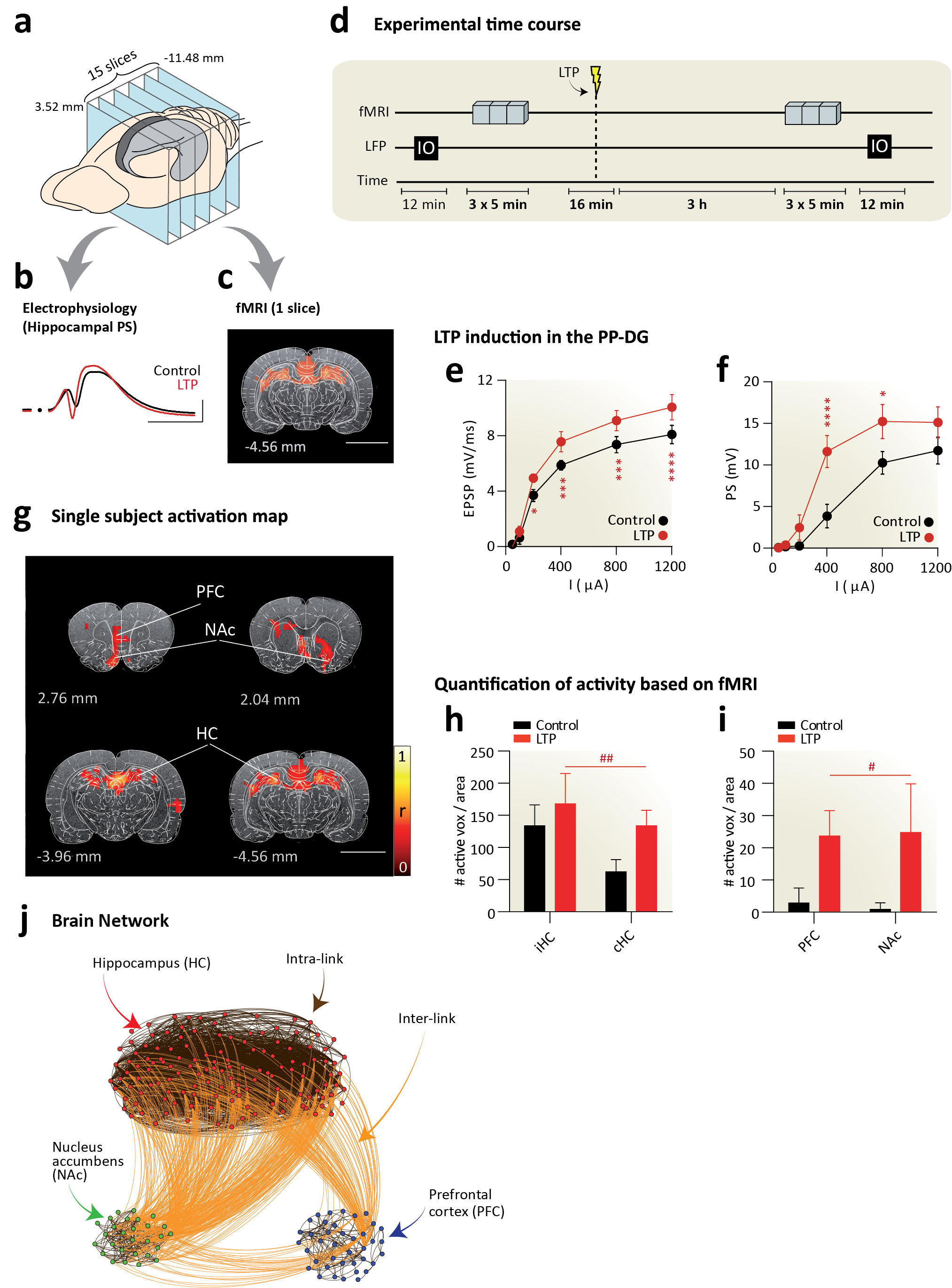
We follow a well-characterized protocol to induce LTP (details of experiments in Fig. 1a-d and Supplementary Note 2) and apply high-frequency pulsed stimulation (250 Hz) of the perforant pathway of the HC in six rats. We apply low-frequency stimulation (10 Hz) before (PRE) and three hours after (POST) LTP induction, to evoke activity in the hippocampal formation while concurrently performing fMRI. Low-frequency stimulation does not affect synaptic efficacy but does allow us to measure activated brain areas with fMRI (e.g. Fig. 1c shows response to stimulation relative to baseline at $p<0.001$, corrected). We verify that synaptic potentiation is induced by the high-frequency stimulation by measuring the concomitant electrophysiological recordings from the dentate gyrus as shown in Fig. 1b, e, and f.

LTP induction results in the propagation of evoked fMRI activity to a long-range functional network beyond the site of low-frequency stimulation (ipsilateral HC). Activations after LTP induction (POST) are reported in Fig. 1g for a single animal, and in Supplementary Fig. 1a for the average over six animals. Compared to the baseline activation (PRE), we see enhanced bilateral fMRI activation of the HC, and activation in frontal and prefrontal neocortical regions (PFC), as well as the nucleus accumbens (NAc) (see Fig. 1h, i for group results and statistics; see also Supplementary Note 2). Conversely, low-frequency stimulation of the perforant pathway before LTP induction produces no fMRI activity in the prefrontal cortex nor in the nucleus accumbens (Fig. 1i).

Generate a brain network model

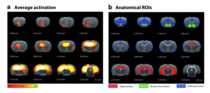
The voxels with significant fMRI activation (due to the low-frequency probe after LTP induction), form the nodes of the network model (see Supplementary Note 3 for details). We focus on evoked activity as we are interested in propagating functional activity in the memory network, rather than spontaneous resting state activity, which will be discussed further below (Section 2). The fMRI signal of the activated voxels is used to compute a functional connectivity matrix, i.e. pairwise correlations between voxels, separately for each animal. To build the computational model of the functional network we proceed in two steps. First we identify the clusters of nodes associated with different brain areas, and then we determine the “connectivity” between nodes.

It is well established that the functional connectivity matrix exhibits a modular structure, with modules (or clusters of nodes) typically associated with different anatomical brain areas meunier . To identify these modules we follow standard procedures bullmore2009 , namely, the functional connectivity matrix is thresholded and a ‘community detection’ algorithm is applied on this binarized matrix girvan2002 ; newman2004 ; fortunato2010 ; gallos . We also register each brain to a standard anatomical atlas (Paxinos and Watson rat brain atlas paxinos2007 ). With this approach we identified in each of the six animals three dominant clusters of nodes (voxels), which overlap well with the anatomical location of the HC, the PFC or the NAc (Supplementary Fig. 1b).

The conventional approach to generating a “connectivity” matrix in brain networks models is to directly threshold the fMRI correlation matrix bullmore2009 . However, correlations do not only arise because two nodes exchange information or are directly linked, but may arise due to common covariates. Furthermore, “spurious connections” may result from a small sample size of the time series used to compute correlations. To minimize the effects of indirect covariation and sampling noise we use a well establish statistical inference method glasso . This method models the observed correlations as the result of direct pairwise interactions, and imposes a penalty to avoid negligible interactions. By varying a penalization parameter, this widely used approach tunes the sparsity of the network. As with the direct thresholding of the correlation matrix bullmore2009 ; gallos ; fallani2017 , there are various ways to select this penalization parameter. We are interested in the formation of a connected brain network, where the different brain areas are linked with each other. Mathematically, this corresponds to the emergence of the “giant connected component” covering the entire network, i.e. all the nodes are connected through a path gallos ; morone2 . We selected the penalization parameter that results in the sparsest network which still exhibits a giant connected component (see also Supplementary Note 3 for details).

In the following, the connections within each cluster are referred to as intra-links, descriptive of short-range interactions within nodes in the same sub-network guimera . Connections between nodes belonging to different clusters are named inter-links, or weak-links gallos , reflecting the long-range interactions between different sub-networks. Inter-links between the HC, NAc and PFC bind these networks into a unified brain network as seen in Fig. 1j for a typical rat (inter- and intra-links shown in orange and black, respectively) gallos ; reis ; morone2 . Once the network model has been constructed, we proceed to identify the essential nodes for integration.

Identifying essential integrators in the brain network model

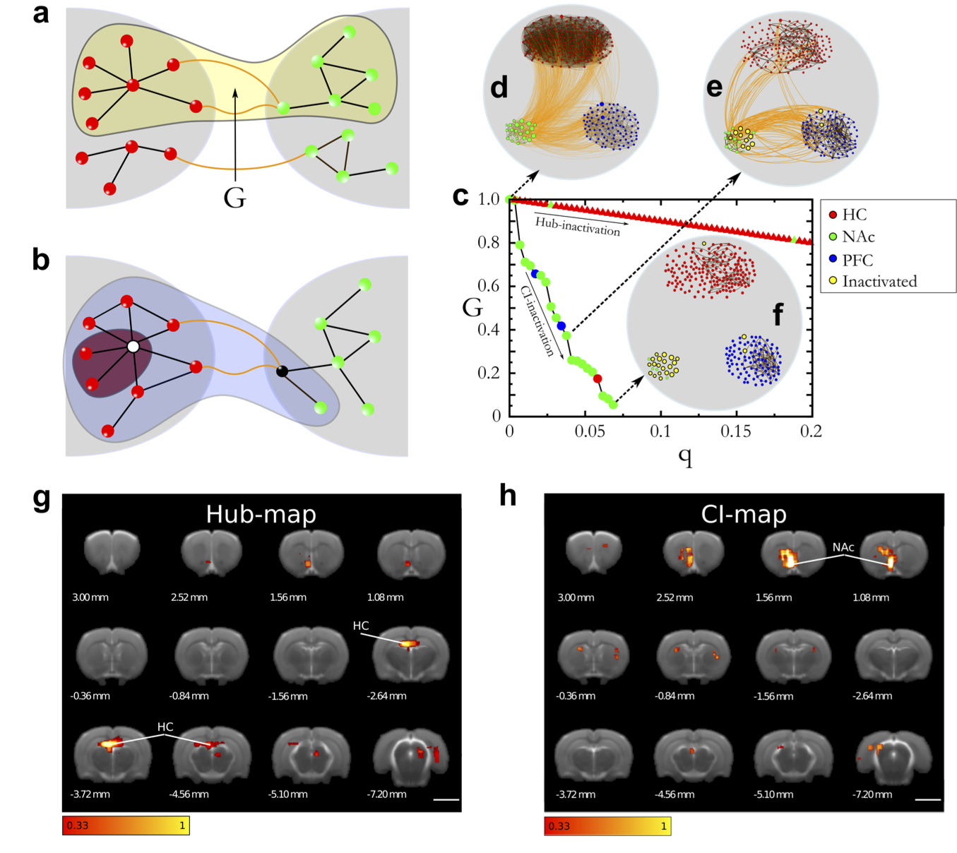
We define global integration as the formation of the largest connected component of nodes in the network – the “giant connected component” $G$. This is the graph that connects the largest numbers of nodes through a path (highlighted in yellow in Fig. 2a; see Supplementary Note 3). The emergence of such a giant component is an important concept in percolation theory, which studies the behavior of clusters in networks as a function of a thresholding parameter of the graph  erdos ; newman-random . The essential integrators of the brain network are then the optimal set (minimal number) of nodes that, upon inactivation, lead to a disintegration of the giant component into smaller disconnected clusters. This is the problem of optimal percolation, which attempt to find such a minimal set of essential nodes or influencers mm ; morone2 . Therefore, we search for the essential nodes by systematic, numerical inactivation of nodes predicted by optimal percolation theory, while we monitor the size of the giant component.

Inactivation proceeds in rank-order according to different centralities. We first apply the hub centrality and thus sort the nodes by their degree. While the hub-centrality is not optimal, it is interesting to see how the hubs rank in terms of network integration, since they have been identified as central to integration in previous studies. As it is customary in network theory albert ; erdos ; newman-random ; mm ; morone2 , we quantify the damage made to the integration of the brain network by measuring the size of the largest connected component $G(q)$ after we remove a fraction $q$ of nodes, whereby nodes are removed in the order of degree from high to low. Figure 2c shows $G(q)$ under inactivation of a fraction of $q$ hubs (mostly HC nodes in red). The curve indicates that the inactivation of hubs does not propagate the damage to the rest of the network. That is, removal of 20% of hubs reduces the size of $G$ by the same amount to 80% of its original value for this representative animal. Further, almost all the hubs are located in the dentate gyrus of the hippocampus. The hub map averaged over six animals which plots the density of essential hubs in the brain, that is, those hubs that create the largest damage upon inactivation (calculated in Supplementary Note 4) is shown in Fig. 2g and confirms that most of the essential hubs are located at the site of LTP induction in the dentate gyrus. This is not surprising since we stimulate its major input (the perforant pathway) to induce the functional brain network. Inactivating the largest hubs in the dentate gyrus experimentally would trivially disrupt the network formation by directly preventing its local activation, rather than by breaking the integration of the network. Thus, these top hubs are trivial influencers.

To find essential nodes beyond the hubs at the HC, we follow optimal percolation to estimate the minimal set of essential nodes mm ; morone2 by ranking the nodes according to the Collective Influence (CI) algorithm morone2 . We find that the ranking following the CI centrality requires the smallest number of inactivated nodes to break up the giant component since CI arises from a maximization of the damage done to the giant component mm ; morone2 . The CI centrality is defined by Equation (2) in Supplementary Note 1 and quantifies the influence of a node not only by its degree, but also by the degree of nodes located in spheres of influence of size $\ell$ – we refer to this as the sphere of influence ${\rm Ball}(i,\ell)$ of radius $\ell$. Thus, CI can identify also low-degree nodes as influential as long as they are surrounded by high degree nodes in their spheres of influence

As shown in the particular animal in Fig. 2c, the giant component $G(q)$ quickly disintegrates when removing the top CI nodes (mostly NAc nodes in green). This result is consistent across all six animals (Supplementary Fig. 3). In clear contrast to the results obtained for hub-nodes, Figure 2c shows that the removal of a very small fraction of top CI nodes ($\sim$7% of the total) is sufficient to reduce the giant component to 5% of its original size. Crucially, most of the nodes in this influential set are located in the nucleus accumbens as shown in the sequence of network inactivation for this particular animal in Fig. 2d-f. Figure 2h shows the CI-map averaged over six animals, indicating that nodes essential to brain integration are located in the nucleus accumbens according to the CI algorithm. This anatomical location is not predicted by conventional hub centrality since nodes in the nucleus accumbens do not appear among the top hubs (Fig. 2g).

To illustrate the different network properties captured by hubs and collective influence centralities consider Fig. 2b. Removing the node with the largest CI (depicted in black) results in large damage to the giant connected component (shaded in blue). Removing the largest hub (depicted in white) causes relatively less damage (shaded in red). Thus, the different nodes predicted by the hub and CI maps are the result long-range influence encoded in the CI measure which is not captured by the local measure of degree. We note that the collective influence centrality includes the hub centrality as the zero order approximation when we take a sphere of influence of zero radius, $\ell=0$ in Supplementary Eq. (2). In this case, the influence centrality of Eq. (2) measures the number of connections of each node. When $\ell\geq 1$, CI captures effects emerging from the long-range structure.

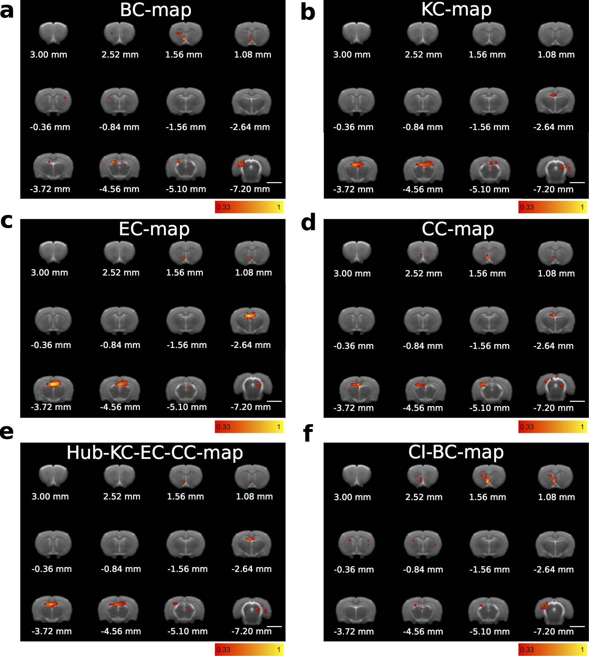
The anatomical localization of essential nodes predicted by the other centrality measures is shown in Fig. 3. A detailed definition of these centrality measures is provided in the Supplementary Note 1. Betweenness centrality (BC-map, Fig. 3a) shares with the collective influence centrality (CI-map, Fig. 2h) a similar location of essential nodes in the brain, showing that the most influential nodes are located in the NAc shell. This indicates that the influential nodes are also bridge nodes captured by the betweenness centrality.

In contrast, the nucleus accumbens does not appear with high $k$-core centrality kc (KC-map, Fig. 3b), which shows a distribution of essential nodes comparable to the hub map. This indicates that the nodes at the inner $k$-core of the network are correlated with their degree as expected by its definition. The eigenvector centrality (EC-map, Fig. 3c) also shows essential nodes mainly located in the HC, as expected since the eigenvectors of the adjacency matrix are highly localized by the hubs as shown in martin . Finally, the closeness centrality (CC-map, Fig. 3d) shows essential nodes for integration in the HC and in the NAc to a lesser extent.

These results unveil a pattern in which centrality measures dominated by local degree (hubs, k-core, EC) tend to identify essential nodes in the hubs of the hippocampus, since nodes with high degree are mostly located in the hippocampus region. These nodes, in the present experiment are trivially associated to the primary location of stimulation, while centrality measurements that capture long-range influence provide a non-trivial result highlighting the strength of the low-degree nodes at the NAc. The role of the nucleus accumbens, thus, is analogous to a fundamental notion of sociology termed by Granovetter as “the strength of weak ties” granovetter ; gallos , according to which a weak tie (in our case a weak node, i.e. low-degree, in the NAc) becomes a crucial bridge (a shortcut) between the densely knit clumps of close friends (the HC, NAc and PFC). The average map of these two categories is shown in Fig. 3e (hub centric: hub-KC-EC-CC-map) and Fig. 3f (weak-node centric: CI-BC-map). In the Supplementary Note 7 we present the degree distribution of the CI nodes, across animals, and compare it with the distribution of the hubs. Supplementary Fig. 6 illustrates that most of the top CI nodes are low-degree nodes.

Overall, this comprehensive network analysis indicates that the integration among HC, NAc and PFC triggered by LTP induction, critically depends on the NAc, and not only on the largest network hubs at the activation site (HC), a fact that had not previously been recognized. The theory based on weak-node centralities predicts that the NAc is strategically located in the memory network, so that inactivating a small number of its nodes is sufficient to have the largest impact on the global connectivity; a falsifiable prediction that we test next.

Targeted inactivation in-vivo in the real brain network

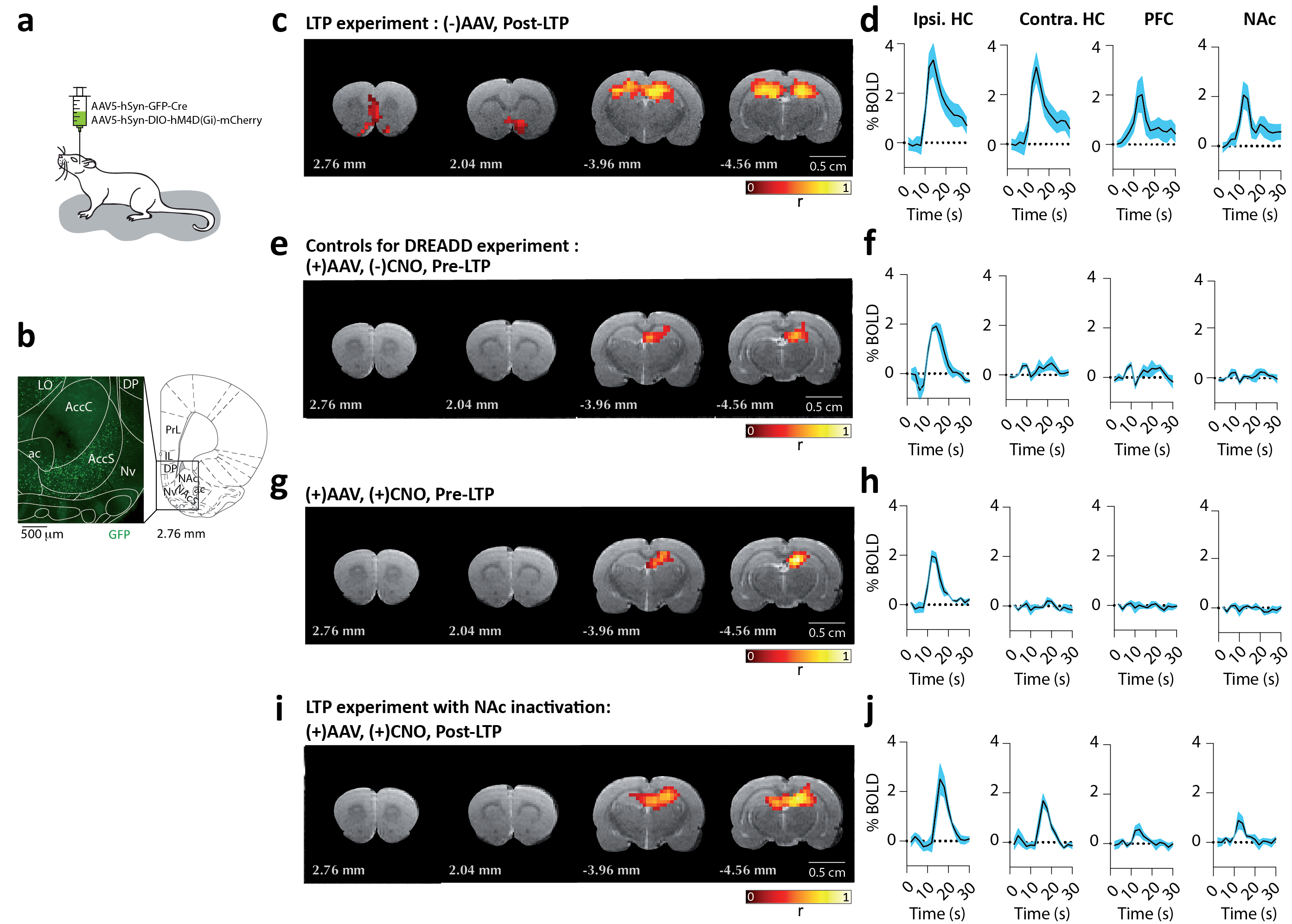
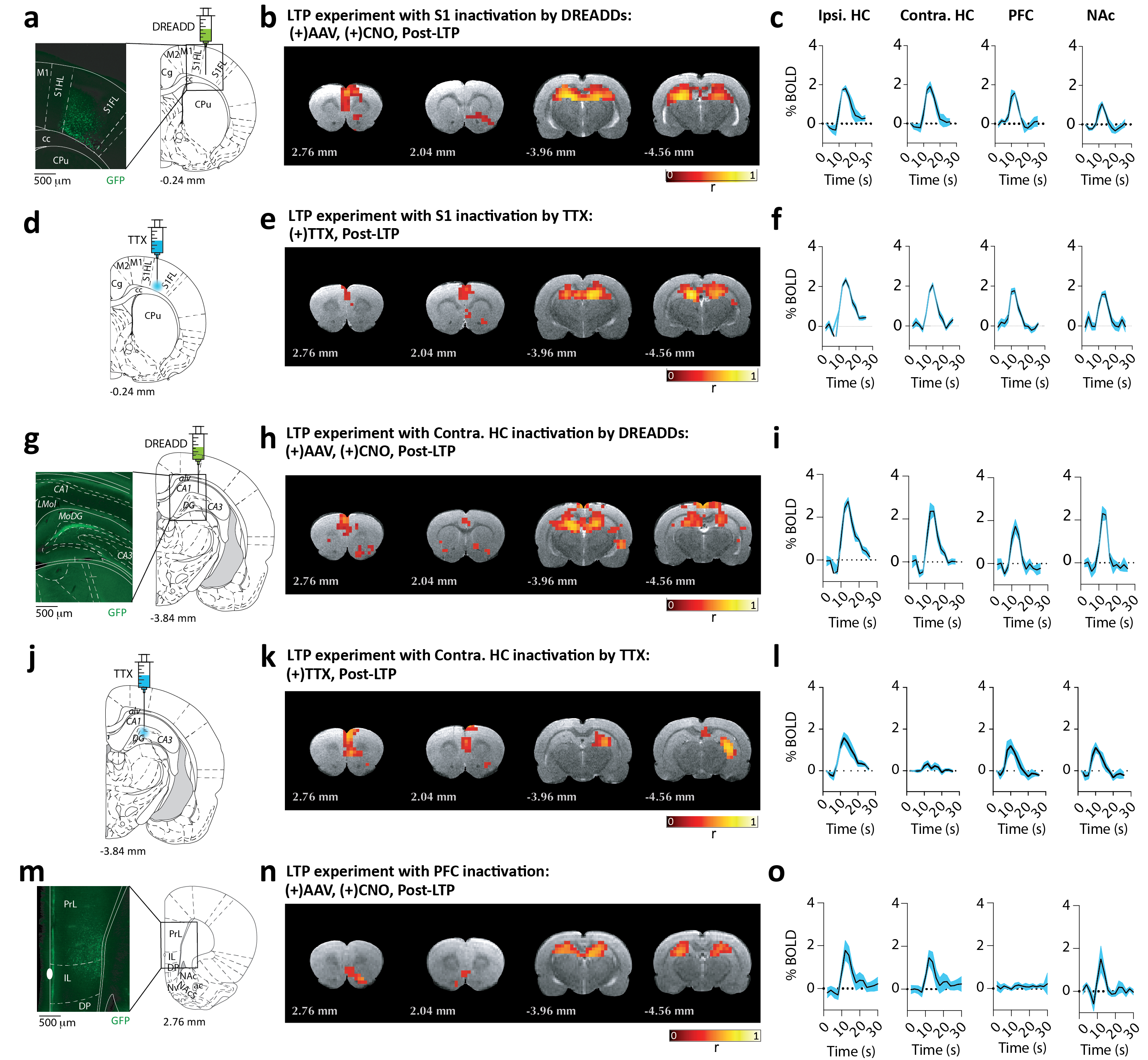
In order to test these predictions, we repeat the LTP experiment in an additional five animals, while inhibiting the activity in the NAc region. The network module identified by the anatomic region in the nucleus accumbens contains 33 nodes in a typical rat, corresponding to a 33mm³ volume. This activated module includes the NAc core and shell (which occupies approximately 10 mm³ in the adult rat) as well as other areas surrounding the NAc. The theoretical prediction of CI identifies the top influencer around coordinate 2.5 anterior and 1.3 mm lateral from bregma and 7.0 mm ventral from the cortex surface, in Paxinos and Watson rat brain atlas space paxinos2007 . This location corresponds to a single node in the anterior half of the NAc shell. The pharmacogenetic intervention infects an approximate volume of 1 mm³, thus silencing a volume corresponding approximately to one to two nodes (voxel volume) in the brain network structure, which allows specific testing of the analytical prediction.

We use adenoassociated viruses (AAV) to direct the expression of Designer Receptors Exclusively Activated by Designer Drugs (DREADDs) roth2016 into the particular targeted area of the NAc shell predicted as the top CI node. More specifically, we use the inhibitory version Gi-DREADD (hM4Di) which, under intra-peritoneal administration of the otherwise inert ligand clozapine-N-oxide (CNO), activates the receptor inducing neuronal silencing and blocking the targeted high-CI node in the NAc shell. With this experimental design, we acquire fMRI data before and after administration of CNO, that is, in presence or absence, respectively, of a functional high-CI node located in the NAc shell of the network.

We favor the pharmacogenetic approach in this experiment over an optogenetic strategy because it avoids implanting bilateral cannula and optic fibers across frontal and/or prefrontal cortical regions from which we collect and analyse fMRI signals. We microinject the viruses bilaterally into the NAc and wait for 4 to 6 weeks to allow strong expression of the construct (see Fig. 4a-b and Supplementary Note 8). Two animals presented infection at neocortical regions due to leak of viral particles during the injection procedure and are not considered in further fMRI analysis. Histological verification demonstrates that viral expression is restricted to approximately a voxel in the shell part of the NAc (Fig. 4b). This subregional specificity is most likely produced by the virus serotype used (AAV5) and gives us the opportunity to selectively silence nodes in the NAc region receiving most HC input groenewegen1991 .

Before LTP induction, we perform a control experiment to inactivate the NAc shell. Comparing before and after CNO administration, (+) and (-) respectively, we find a comparable fMRI response to low-frequency stimulation in the hippocampus: Both the fMRI activation maps (Fig. 4e, g) and the amplitude of the fMRI signals averaged across animals (Fig. 4f, h) are unchanged, demonstrating that the baseline fMRI response in the HC is not altered by NAc shell inactivation. Therefore, the input necessary to drive the formation of the memory network is preserved and can be used to experimentally test the theoretical predictions.

Using the same animals, we induce LTP in the perforant pathway as before but, this time, under inactivation of the NAc shell ((+) CNO). Figure 4i, j shows that, as predicted by the theory, the formation of the long-range network involving HC, PFC and NAc is completely prevented, yet LTP induction still produces the expected potentiation of the intra-hippocampal bilateral activation (compare Fig. 4g, h and 4i, j). Remarkably, long-range inter-network links from the HC to the PFC are not formed (Fig. 4i, j), even though these sub-networks are not directly inactivated.

For comparison, the result of LTP induction in animals with a fully active NAc (animals without DREADD expression, (-) AAV) is shown in Fig. 4c demonstrating ipsilateral and contralateral HC activation together with PFC and NAc in response to the perforant pathway stimulation (Fig. 4d). These results demonstrate that inactivation of the highest CI node in the NAc shell disrupts the formation of the memory network by selectively blocking the formation of LTP-dependent connections to neocortical structures, but not the local potentiation of hippocampal synapses.

Control experiments: in-vivo inactivation of brain regions predicted to have no effect

To further validate these results, we perform a series of in-vivo inactivation experiments targeting nodes which, based on our model predictions, should have no major effect on the long-range functional network.

We start with the inactivation of a node in the primary somatosensory cortex (S1), a brain region outside of HC-PFC-NAc functional network. Inactivation is first performed using DREADDs as before, with virus injection targeting the S1 region (Fig. 5a, see Supplementary Note 8 for details). As shown by the activation maps and fMRI signals in Fig. 5b-c, S1 inactivation does not prevent the LTP-induced activation of the HC-PFC-NAc network. Furthermore, in an additional group of animals we increased the strength of inactivation in S1 cortex by infusing 0.5 $\mu$L of tetrodotoxin (TTX, 100 $\mu$M) at the same stereotaxic coordinates (Fig. 5d). TTX is a sodium channel blocker that completely blocks neuronal firing at these concentration (see Supplementary Note 9 for further details). Still, Fig. 5e-f demonstrate HC-PFC-NAc network formation upon LTP induction in these conditions.

Inactivation of the HC ipsilateral to the stimulation site would trivially eliminate the long-range network preventing its initial activation. We therefore tested whether inactivation of the contralateral HC nodes, identified by our model as non-essential nodes for global integration, would preserve network formation. As for S1 cortex, we used DREADDs (Fig. 5g) and TTX (Fig. 5j) in separate experiments to assure strong and wide inactivation of the contralateral HC (see Supplementary Note 8 and 9, for details). The results with both manipulations verify our model prediction by showing successful LTP-induced formation of a long-range HC-PFC-NAc network under contralateral HC inactivation (Fig. 5h-i and 5k-l). Note that TTX injection prevents the activation of the complete contralateral HC, involving a large number of network nodes but nonetheless, the long-range network is preserved.

In our final control experiment we targeted the DREADD inactivation to the anterior part of the PFC (Fig. 5m), a central part of the long-range network for which our model predicts low impact on global integration. TTX is not used for this target because the close proximity of the NAc and the diffusion of the TTX solution after injection cannot exclude direct inactivation of the NAc (and vice versa). However, the pharmacogenetic manipulation was enough to inactivate the PFC as demonstrated in the fMRI activation map and corresponding BOLD signals (Fig. 5n-o). Most importantly, under PFC inactivation, LTP successfully recruits the long-range HC-NAc network.

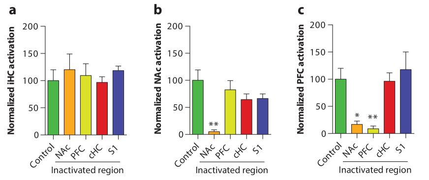
Between-groups statistical comparison (Fig. 6, see caption for statistics) demonstrates that only NAc inactivation promotes the complete disintegration of the LTP-induced HC-PFC-NAc network, while PFC targeting only produces the expected inactivation of the PFC and control S1, and contralateral HC inactivations preserve the complete long-range integrated network. Overall, these results lend strong support to the predictive validity of the model and the key role of the NAc in the LTP-induced long-range functional network.

Network analysis of the Resting State dynamics

As already indicated, the formation of the HC-PFC-NAc network is contingent on LTP induction. Accordingly, prior to LTP induction, the low-frequency stimulus that probes network function, exclusively activates the HC, but neither PFC nor NAc are activated and, therefore, the relevance of these structures in the PRE-LTP condition cannot be studied during hippocampal stimulation.

To shed light on the role of these brain areas before LTP induction we analyze resting-state fMRI data. From the fMRI signal prior to LTP, and in the absence of the low-frequency probing stimulus, we build a resting-state brain network for each of the six animals, by using the same network construction procedures as before. We then use CI centrality to rank the nodes according to their importance for brain integration, as we did for the LTP-induced functional network. Further details on the procedure are discussed in Supplementary Note 5 and an averaged CI-map over the six rats is shown in Supplementary Fig. 4. These findings should be compared with Fig. 2h which presents the same type of results for the functional network induced by LTP.

The outcome illustrate that, the nucleus accumbens does not always play an essential integrative role. On the contrary, the importance of the NAc arises here as a result of LTP induction. In contrast, during resting state dynamics, nodes with high CI are distributed among different brain areas (see Supplementary Fig. 4). Therefore, the integrative role of the nucleus accumbens is specifically related to synaptic plasticity in the memory network.

Caveat on the methodology: from undirected to directed brain networks

Key to our reasoning is that integrating information of specialized local modules into a global network is crucial for brain function. So far, this integration was modelled and measured as long-range correlated fMRI activity. However, these correlations do not necessarily measure direct interactions between neural populations through fibers, the so-called structural network. Some correlations may result from indirect covariations that do not reflect direct communication between nodes. To minimize effects due to this indirect covariations (i.e., high correlations between two nodes that are indirect since they do not come from a direct fiber structural connection between the nodes) we use a statistical approach (glasso) glasso which attempts to explain the observed correlations as result of pairwise interactions. However, this model assumes undirected (symmetric) interactions. Measuring information exchange, on the other hand, needs a potentially asymmetric estimate that excludes some non-causal correlation, e.g. Granger Causality granger , which result in directed (asymmetric) interactions.

To determine if our results are robust when directed interactions are considered, we repeated the network analysis by endowing the network with directed links. For each pair of voxels in the HC-PFC-NAc network, we determine connectivity as before (Sec. 2) and, in addition, we measure Granger causality to determine the direction of the link. The final wiring of this directed network graph for each animal is different from the wiring of the undirected network (see Sec. 2). Remarkably, by computing the CI centrality on these directed networks (see Sec. 2 and Supplementary Note 6 for details), the main results regarding the location of the influential nodes is preserved: most influential nodes are located in the nucleus accumbens and they are low-degree nodes, see Supplementary Fig. 5 in Supplementary Note 6. These results further strengthen our previous findings on the role of the NAc in the HC-PFC-NAc integration.

3 Discussion

While a fundamental role of the NAc in the meso-cortico-limbic system has long been recognized, including for memory lisman2005 ; pennartz2011 ; floresco2015 , our results suggest a new role for the NAc function in this system. The NAc receives major excitatory inputs from PFC and HC and dopaminergic inputs from the ventral tegmental area (VTA), among others groenewegen1991 ; floresco2015 . These anatomical, but also neurophysiological and behavioural evidences pennartz2011 ; floresco2015 , have favored the view of the NAc as a downstream station in this circuit, working as a limbic-motor interface with a role in selecting behaviorally relevant actions mogenson1982 . Human and animal studies further indicate that in addition to performing on-line processing for action selection, the NAc encodes the output of the selected action (positive or negative relative to expectation) into memory, which in turn will condition future selections floresco2015 ; pennartz2011 . In this context, however, our network analysis locates the NAc upstream in the circuit, showing that interactions between the HC and PFC induced by LTP are already under the control of the NAc. Being the interaction between these two structures key for memory formation, we interpret our results as indicative of a NAc-operated gating mechanism that couples HC-PFC networks for the storage of new information, providing a mechanism for updating memories to guide future behaviors. This mechanism would fundamentally differ from, but being compatible with, previous ideas on information flow between HC, PFC and NAc networks Grace in that the control here is exerted bottom-up from the NAc. While the precise mechanism for this control switch has not been investigated in the present work, an appealing possibility is the regulation of neuronal excitability in the ventral tegmental area (VTA) by projections of the NAc shell through the ventral pallidum lisman2005 . In turn, dopamine release from VTA terminals in the HC and neocortex would promote synaptic plasticity and facilitate integration in a consolidated memory brain network. Regardless of the specific microcircuit, in this network-driven theory, NAc computations seem to be a necessary part of hippocampal-dependent memories.

The experimental model used in this work leverages the induction of LTP in the dentate gyrus, which leads to a large-scale network that we could perturb prospectively. The experimental finding highlights the importance of considering the entire network associated with each node. Network hubs, defined solely by the number of direct connections, are not necessarily the the most effective at channeling information through the entire network. This role may be reserved for essential nodes that connect different communities to each other power2013 . The collective influence centrality use here accounts for the role of nodes in connecting different brain areas to one another mm . Thus, this approach extends beyond the direct effects of hubs at integrating brain networks.

This result has important implications for the numerous investigations on brain pathology searching for critical alterations in functional connectivity as disease diagnostic and/or prognostic biomarkers. A combination of optimal percolation theory and experimental test presented here can be potentially adapted to networks that do not depend on LTP induction for their formation, thus providing a recipe to design intervention protocols to manipulate a wider range of brain states. These may include stam : (i) transcranial magnetic stimulation that can stimulate or deactivate focal brain activity, (ii) assist in targeting deep brain stimulation devices, in particular, for disorders that are thought to be the result of network dysfunctions, and (iii) guiding brain tumor surgery by identifying essential areas to be avoided during the resection. The basic hypothesis is that activation/deactivation patterns applied to the influential nodes will propagate through the brain to impact global network dynamics. The proposed theoretical analysis provides a possible road map on how to establish and test such basic network hypotheses.

To conclude, we mention that our analysis was based only on correlation structure of evoked fMRI. Future work could study the network structure and the role of node’s degree in connectome data oh2014mesoscale ; barabasi . It would be important to compare the role of hubs, weak nodes, and nodes connecting different modules in structural brain networks with their role in functional networks. Such investigations, together with those presented in this work, are of crucial importance for diagnostic and clinical intervention in the brain.

Data availability

Data that support the findings of this study are publicly available and have been deposited in http://www-levich.engr.ccny.cuny.edu/webpage/hmakse/software-and-data/

Acknowledgements

This work was supported by NIH-NIBIB 1R01EB022720, NSF IIS-1515022, NIH-NCI U54CA137788/ U54CA132378, NSF PHY-1305476 and by MINECO and FEDER Grants BFU2015-64380-C2-1-R, EU Horizon 2020 Grant No 668863 (SyBil-AA), and Spanish State Research Agency, through the “Severo Ochoa” Program for Centers of Excellence in R&D (ref. SEV-2013-0317). Ú.P.-R. was supported by MECD Grant FPU13/03537. The authors are grateful to B. Fernández for technical assistance and K. Roth for discussions.

Author contributions

All authors contributed to all parts of the study.

Additional information

Supplementary Information accompanies this paper at http://www.nature.com/naturecommunications

Competing interests: The Authors declare no Competing Interests.

Correspondence and requests for materials should be addressed to S.C and H.A.M.

FIG. 1. Experimental protocol and generation of brain network.

a, Schematic representation of the imaging planes (blue). The hippocampus (HC) is highlighted in grey. Numbers indicate z coordinate in mm from bregma. b, representative evoked population spike (PS) in the dentate gyrus before (black) and after (red) LTP induction. c, representative fMRI maps across the HC during perforant path stimulation overlaid on an anatomical T2-weighted image with atlas parcellations (see Supplementary Note 2). Color indicates significant correlation ($p<0.005$ corrected). d, Time course of the experiment. Input/output (I/O) response curves are recorded in the local-field potentials (LFP). fMRI signals are collected during low frequency (10 Hz) test stimulations before and 3h after LTP induction. e, Field excitatory postsynaptic potential (EPSP) slope and, f, population spike (PS) amplitude before (black) and after (red) LTP. Two-way repeated measures ANOVA ($n=5,\alpha=0.05$) reveals significant effects of LTP in both measures ($F_{1,24}=27.82,\,p<0.0001$, and $F_{1,24}=59.89;\,p<0.0001$ for PS and EPSP, respectively). Mean $\pm$ SEM. Post-hoc Bonferroni: ${}^{*}\,p<0.1;\,^{**}\,p<0.01;\,^{***}\,p<0.001;\,^{****}\,p<0.0001$ g, Representative fMRI maps in one animal after LTP induction. Color code as in panel c ($p<0:005$; see Supplementary Note Fig. 1 for group activation maps and Supplementary Note 2 for details). Size bar corresponds to $0.5$ mm. h, i, Number of active voxels per selected region in control (black) and LTP (red) conditions in hippocampal (h) and extra-hippocampal areas (i). The stimulated region is the ipsilateral hippocampus (iHC); two-way repeated-measures ANOVA ($n=7,\alpha=0.05$) reveals significant effects for LTP in hippocampal ($F_{1,12}=15.72,{\small\#\#}\,p=0.0019$) and extrahippocampal regions ($F_{1,12}=7.426,{\small\#}\,p=0.0184$), with no interaction between regions ($F_{1,12}=0.00242,\,p=0.9616$ and $F_{1,12}=1.518,\,p=0.2415$ for hippocampal and extra-hippocampal regions, respectively). Mean $\pm$ SEM. h, Brain network formed by the HC, NAc and PFC for the animal in g. The brain network is formed by intra-network interactions and inter-network interactions inferred from fMRI correlation data (Supplementary Note 3).

FIG. 2. Hub and Collective Influence map. a, The giant (largest) connected component $G$ (yellow), captures the integration of two modules into a brain network. b, Influence of a hub and a CI node. Inactivation of the hub (white node) produces less damage to brain integration, measured by the size reduction of $G$, then the inactivation of the CI node (black). c, Relative size of $G$ as a function of the fraction of inactivated nodes, $q$. Two strategies are shown for choosing the essential nodes in a representative animal: Hub-inactivation (triangles) and CI-inactivation (circles). Nodes are removed one by one according to their degree or CI-score, respectively, from high to low. Colors refer to the node s module (HC, NAc, or PFC, see legend). Most hubs (red symbols) are located in HC, yet, they are not essential for integration: their removal makes minimal damage to $G$. On the contrary, by inactivating 7% of high CI nodes, $G$ collapses to almost zero. Most CI nodes are in the NAc (green symbols). d, Representative brain network as in c, displaying the PFC-HC-NAc networks. The size of each node is proportional to the CI-score. e, We inactivate the top 3% of high CI nodes (yellow circles) and $G$ is drastically reduced to less than 40% of its original value. These top CI nodes are all in the NAc except for two nodes in the PFC. f, Further inactivating up to 7% of the high CI nodes prevents integration of $G$. Yellow circles indicate the essential nodes, located mostly in the NAc shell. g, Average hub map indicating top hub nodes over six animals. Yellow/white areas correspond to top essential nodes all located in the HC since this is the area of LTP induction. Color bar represents the average rank (Supplementary Eq. (8)). h, Average CI map indicating top CI nodes over six animals, most CI nodes results in the NAc and are generally not hubs. Color bar is defined in Supplementary Eq. (8), the size bar corresponds to $0.5$ mm.

FIG. 3. Maps of essential nodes. Average map of influencers for the different centralities according to a, betweenness centrality, b, $k$-core centrality, c, eigenvector centrality and d, closeness centrality. The maps are average over the six rats and the color bar are calculated according to the rank defined by Supplementary Note 4, Eq. (8). Yellow/white colors indicate the top influencers according to each centrality. According to these results, the centralities are then divided into e, hub-centric centralities dominated by the hubs and identifying the hubs in the HC and f, integrative centralities dominated by the weak nodes and identifying the low degree nodes in the shell part of the NAc. The size bar in each panel corresponds to $0.5$ mm.

FIG. 4. Experimental test of essential nodes. a, The inhibitory version of DREADD receptors (hM4Di) is expressed in the NAc shell using a combination of two adenoassociated viruses (AAVs) injected stereotactically in the region as indicated (see Supplementary Note 8 for details). b, Histological verification 4 weeks after the viral infection showing green fluorescence protein (GFP) in the neurons that positively express the construct. For anatomical reference, an image of the rat brain atlas is shown. Inset: 20x magnification picture of the same slice demonstrating selective infection of neurons in the NAc shell. c, e, g, i: single subject statistically thresholded fMRI maps showing voxels activated ($p<0.001$, corrected) by perforant path stimulation and overlaid on an anatomical T2-weighted image. d, f, h, j: BOLD time courses from significantly activated voxels averaged from the indicated regions of interests and across animals (mean $\pm$ SEM; $n=6$ for panel c, $n=3$ for panels e, g and i). Details on fMRI processing and statistics are given in Supplementary Note 2 and 8. c, LTP experiment for comparison ((-) AAV infection, (-) CNO administration) showing the expected activation of HC, PFC and NAc in POST-LTP. Note the evoked BOLD responses bilaterally in the HC (panel d), a landmark of HC response after LTP induction. e, AAV infection in the NAc ((+) AAV, (-) CNO) preserves activation of the HC under perforant path stimulation before LTP. g, Inactivating the NAc by administration of CNO in the same animal ((+) AAV, (+) CNO) does not alter functional maps nor BOLD responses in the baseline (PRE-LTP) condition (compare e vs g). BOLD signal responses (f, h) are only evident in the ipsilateral HC as expected from PRE-LTP condition. i, j, NAc inactivation ((+) AAV, (+) CNO) prevents the integration of the long-range network involving HC-PFC-NAc induced by LTP (POST-LTP).

FIG. 5. Targeted inactivation of different brain regions. a, b, c, Pharmacogenetic inactivation of S1 cortex. a, location of the AAVs injection in the corresponding section of the stereotaxic map and representative histological staining showing the construct expression (inset). b, shows the statistically thresholded ($p<0.001$, corrected) fMRI maps of a representative animal and c, the averaged BOLD signals across subjects ($n=2$) and across region of interest. As in Fig. 4, S1 inactivation does not disrupt the long-range network formed upon LTP induction. d, e, f, Inactivation of S1 with TTX (See Supplementary Note 9, for experimental details). Same as a-b-c experiments with S1 inactivation using the sodium channel blocker TTX ($n=3$). Both fMRI maps and BOLD signals demonstrate formation of the HC-PFC-NAc network triggered by LTP ($p<0.001$). g-l, Pharmacogenetic (g, h, i, $n=5$) and TTX (j, k, l, $n=4$) inactivation the contralateral HC ($n=5$). As shown in the individual fMRI maps and averaged BOLD signals ($p<0.001$), none of the inactivation strategies targeting the contralateral HC prevented the formation of the HC-PFC-NAc network. m, n, o, Pharmacogenetic inactivation of the PFC ($n=5$). AAVs injection targeted to the anterior part of the PFC (m) prevents its activation by performant path stimulation, as expected by the pharmacogenetic intervention, but does not abolish the formation of the long-range HC-NAc connections ($p<0.001$), as predicted by the theory (n, o).

FIG. 6. Group analysis of network inactivation. The number of nodes in the relevant networks is quantified after LTP induction with or without targeted inactivation and normalized relative to the control, fully active, condition. a, Proportion of nodes recruited by perforant pathway stimulation in the ipsilateral HC under control conditions (100%) and after inactivation of the NAc, PFC, contralateral HC (cHC) and S1, as indicated in the $x$-axis. Analysis of variance across groups demonstrates no statistical differences (ANOVA, $F_{4,24}=0.3641,p=0.8317$). b, Proportion of nodes recruited in the NAc following targeted inactivation in the structures indicated in the $x$-axis. ANOVA demonstrates statistically significant differences between groups ($F_{4,24}=4.841,p=0.0053$) and post-hoc Bonferroni test finds the only significant difference in NAc recruitment when the NAc is directly inactivated ($p<0.01$), as expected from the experimental manipulation, but no effect under PFC, cHC or S1 inactivation. c, Proportion of nodes recruited in the PFC following targeted inactivation in the structures indicated in the $x$-axis. ANOVA demonstrates statistically significant differences between groups ($F_{4,24}=6.416,p=0.0012$) and post-hoc Bonferroni test identifies strong reductions in both PFC ($p<0.01$), expected from the experimental manipulation, but also NAc ($p<0.05$), indicating the disintegration of the long-range HC-PFC-NAc network under NAc inactivation.

Figure 1:

Figure 2:

Figure 3:

Figure 4:

Figure 5:

Figure 6:

Supplementary Information

Finding influential nodes for integration in brain networks using optimal percolation theory

Del Ferraro et al.

1 Finding the essential nodes for integration in the brain network

In this section, we provide the heuristic algorithms used to identify influential nodes. For each algorithm, we assign the score to each node by following the described algorithms and sort the nodes according to the score.

Degree centrality. Degree centrality is the number of nearest neighbors in the network. Degree centrality is one of the simplest metric for identifying important nodes. Hubs refer to nodes in the network with large degree.

$k$-core and $k$-shell index seidman ; kc ; hagmann . $k$-core (KC) refers to a subset of nodes formed by iteratively removing all nodes that have degree less than $k$. In other words, $k$-core is a maximal subgraph where all nodes have at least $k$ neighbors. $k$-shell index is then the largest $k$ value of $k$-core that the node belongs to. To assign $k$-shell index for each node, we first delete all nodes with degree $k=1$, iteratively. The removed nodes via the process belong to $k$-shell with $k_{S}=1$. We remove next $k$-shell with $k_{S}=2$ and we proceed to remove all the higher shells iteratively until all nodes are removed. Then, we can assign a unique $k$-shell index to each node in networks. It has been shown that the importance of hub nodes can be highly diminished if they are located in the periphery of the network, i.e., the low $k_{s}$ shells. On the other hands, nodes in the inner $k_{s}$ shells define the core of the network and correspond to the influencers in the network kc . However, by its own definition, the nodes in the inner shells are generally high degree nodes, therefore the $k$-core centrality is highly correlated with the degree.

Collective Influence mm ; morone2 . Collective influence (CI) is designed to approximately identify the minimal set of nodes that can produce disconnected networks, based on optimal percolation network theory mm . Mathematically, the problem can be mapped to optimal percolation and can be solved by the minimization of the largest eigenvalue of the non-backtracking matrix of the network mm ; morone2 . This optimization theory was originally developed for single networks in mm and was extended to the case of brain networks in morone2 in the context of brain network of networks. The activation of nodes in the brain network was described by a state variable $\sigma_{i}$, which acts as an ON and OFF switch ($1$ and $0$, respectively) to reflect the activation/inactivation state of node $i$. If a node is directly inactivated, then $\sigma_{i}=0$. A node can also be inactivated indirectly as a result of lacking input from its inactivated neighbors in the other network, which, mathematically, is equivalent to the McCulloch-Pitts model of neuronal activation mcp :

$$\sigma_{i} =\ 0\ \ \ {\rm direct\ inactivation}\ ,$$ (1)

$$\sigma_{i} =\ \Theta\Bigg{(}\sum_{j\in\mathcal{N}(i)}\sigma_{j}\Bigg{)}\ \ \ {\rm otherwise}.$$

The sum in the second equation reflects the integration of incoming activity from all nodes $j$ that connect to node $i$ from other networks $\mathcal{N}(i)$, and the threshold operation via the Heaviside step function $\Theta$ indicates that a minimum of incoming activity is needed for activity to propagate mcp .

The collective influence (CI) score assigned to each node $i$ in the brain network in this model is given by morone2 :

$${\rm CI}_{\ell}(i)=(k_{i}-1)\sum_{j\in\partial{\rm Ball}(i,\ell)}(k_{j}-1)+\sum_{\begin{subarray}{c}j\in\mathcal{F}(i)\ :\\ k_{j}^{\rm inter}\ =1\end{subarray}}(k_{j}-1)\sum_{m\in\partial{\rm Ball}(j,\ell)}(k_{m}-1).$$ (2)

Here, $k_{i}\ \equiv\ k_{i}^{\rm intra}+k_{i}^{\rm inter}$ is the degree, $k_{i}^{\rm intra}$ is the number of connections of node $i$ within its network, $k_{i}^{\rm inter}$ is the number of connections to nodes in different networks in the set $\mathcal{F}(i)$, and $\partial{\rm Ball}(i,\ell)$ indicates the sphere of influence of node $i$ at distance $\ell$.

Technically, CI is the contribution of each node to the eigenvalue of the non-backtracking matrix, which determines the stability of the giant component mm . CI is an optimization measure that attempts to find the smallest set of nodes that will produce the largest damage to the giant connected component of the brain network, which is analogous to minimize the largest eigenvalue of the non-backtracking matrix mm defined on the $2M\times 2M$ edges of the network (in the case of single networks):

$$\mathcal{B}_{k\to\ell,i\to j}=\begin{cases}1,\,\,\,\,\mbox{if}\,\,j=k\,\,\,\,\mbox{and}\,\,\,i\neq\ell\ ,\\ 0,\,\,\,\,\mbox{otherwise}.\end{cases}$$ (3)

Thus, the matrix $\mathcal{B}_{k\to\ell,i\to j}$ has non-zero entries only when $(k\to\ell,i\to j)$ form a pair of consecutive non-backtracking directed edges, i.e. $(k\to\ell,\ell\to j)$ with $k\neq j$. In this case $\mathcal{B}_{k\to\ell,\ell\to j}=1$. The powers of the matrix $\hat{\mathcal{B}}$ give the number of non-backtracking walks of a given length between two nodes in the network hashimoto ; nbt , in analogy to the powers of the adjacency matrix which count the number of paths newman-book .

The CI algorithm runs as follows morone2 : i) at the beginning, we choose the value $\ell$ of the radius of the Collective Influence sphere. In our analysis of the brain network, we use the value $\ell=2$. We find that higher values of $\ell$ give nearly the same results since the networks contain short paths. The value of $\ell$ is always smaller than the largest path in the network, and it can be optimally chosen by systematically changing it from $\ell=1$ to the diameter of the network. We find that the optimal set of nodes is obtained when $\ell=2$. ii) Next, CI for all nodes is computed using Eq. (2), and the node with the largest CI is inactivated. iii) Then, the CI values of the remaining active nodes are recalculated, and the next highest CI node is inactivated. iv) Step iii) is repeated until the giant active component vanishes.

Betweenness centrality BC . Betweenness centrality (BC) measures the influence of nodes based on the shortest paths on networks. BC for each node is defined as the number of the shortest paths that pass through the node. BC identifies crucial nodes for information flow and packing transportation by definition. This centrality can capture low-degree nodes that are strategically located between large communities. For instance, imagine a node with $k=2$ with each link connecting to a large community of tightly connected nodes. Such a low degree node will have a large BC since all the paths between nodes in the two distinct communities will necessarily pass through this bridge node.

Eigenvector centrality EC . Eigenvector centrality (EC) is defined as the entry of the eigenvector that corresponds to the largest eigenvalue of adjacency matrix defined as

$$A_{ij}=\begin{cases}1,\,\,\,\,\mbox{if}\,\,i\,\,\,\,\mbox{and}\,\,\,j\,\,\,\,\mbox{are connected}\\ 0,\,\,\,\,\mbox{otherwise}.\end{cases}$$ (4)

The main idea of EC is that the influence of nodes is determined by the importance of its neighbors. Therefore, neighbors with high-scoring eigenvector centrality more contribute to the score of the node. PageRank is also a variant of EC. It has been proved in martin that the use of the largest eigenvalue of the adjacency matrix can lead to a localization of the influence in the hubs. Thus the EC centrality is highly correlated with the high degree and contains similar information about the influencers. This localization problem is solved by replacing the adjacency matrix in the centrality by the non-backtracking matrix Eq. (3).

Closeness centrality CC . Closeness centrality (CC) is defined as the inverse of the average distance of shortest paths between the node with all other nodes in the network. The higher closeness is, the closer it is to all other nodes in average. In practice, closeness play an important role in transportation since nodes with higher CC can disseminate information efficiently to the whole connected network via shortest paths. This centrality is mainly determined by the degree since hubs will naturally be closers to other nodes in the networks, thus, it is considered as one of the hub-centric centralities.

2 Experimental Design and Long-term potentiation experiments

The brain network is based on long-term potentiation (LTP) experiments. LTP is a synaptic strength modification protocol that leads to changes in neuronal networks, and is believed to be one of the key mechanisms by which the brain undergoes memory processes (acquisition, consolidation, and extinction) bliss ; lynch ; bliss1973 ; bliss1993 ; martin2000 ; morris2001 ; squire1986 . It refers to the enhancement of synaptic transmission efficacy in specific neuronal connections. This mechanism has been observed to occur under natural learning conditions, yet, experimental manipulation of synaptic transmission has allowed deciphering many of its characteristics, dissecting the synaptic plasticity process from other on-going processes during memory formation. In the present work, we use experimental LTP induction in the rat hippocampus to provide an experimental model of controlled long-range functional connectivity reorganization.

All experiments were approved by the Spanish authorities (IN-CSIC), CCNY Institutional Animal Care and Use Committee Review of Research Protocol No. 980, and were performed in accordance with Spanish (law 32/2007) and European regulations (EU directive 86/609, EU decree 2001-486). The data used in this study can be found at: http://kcorelab.org. Details of the experiments are explained in the next sections.

Subjects

A total of 37 Sprague-Dawley male rats, weighing between 250-350 g, were used in these experiments. From these, 29 animals were conserved for data analysis (6 controls for the LTP network generation in baseline conditions, 4 for NAc inactivation with DREADDs, 5 for PFC inactivation with DREADDs, 4 for Hippocampal inactivation with DREADDs, 5 for Hippocampal inactivation with TTX, 2 for S1 inactivation with DREADDs, and 3 for S1 inactivation with TTX. A total of five animals were discarded due to surgery complications or poor quality of MR images, and additional three because of leak of viral particles to the neocortex in the NAc inactivation experiments. Animals were purchased from Janvier Labs (France) and maintained under a 12/12 h light/dark cycle (lights on 07:00-19:00 h) at room temperature (22$\pm$2 C). Food and water were provided ad libitum. Rats were housed in groups (4-5 animals per cage) and adapted to these conditions for at least 7 days before any manipulation.

Surgery and electrode implantation

The animals are anesthetized briefly with isoflurane (3-4 $\%$ isoflurane in 0.8 L/min O2 flow) and then injected intraperitoneally with urethane (1.3 g/kg). After 60 minutes, the main reflexes disappearance is tested and, if necessary, a second dose of urethane is injected (1/5 of the initial dose) as reinforcement. When reflexes disappear the surgery starts. During the complete procedure animals are maintained with constant temperature (37.0-37.5 C) with a water pad. Vital constants (pulse and breath distension, heart and breath rate, and oxygen saturation) are monitored using a paw-clip pulse oximeter (MouseOx Plus, Starr Life Sciences, Oakmont, US). A constant flow of $O_{2}$ (0.8 L/min) is supplied through a mask.

The anesthetized animal is placed in a stereotaxic frame (Narishige, Japan) and a local anesthetic is injected subcutaneously in the incision points (0.2 mL of bupivacaine). The skin is opened and retracted with suture thread hold to haemostat clamps to expose the bone surface. Special care is taken to remove all traces of blood from the skull and mussel that would decrease MRI data quality due to susceptibility artefacts. Care during surgery is maximized to prevent even minor spontaneous bleeding throughout the MRI session which would also distort the BOLD (blood oxygenation level dependent) signal. Trephine holes are made by hand with a manual driller (2 mm diameter) in the target coordinates and the dura is pinched with a curved needle at the incision points to allow the penetration of the electrodes.

A bipolar stimulation electrode made of twisted platinum-iridium wires (Teflon coated, 0.025 mm diameter, WPI, USA) is inserted in the perforant pathway, a bundle of axonal fibers that represents the principal input of information to the hippocampus (AP 0.0 mm from lambda; ML 4.1 mm from lambda; DV 2.1-2.5 mm from brain surface). A recording multichannel electrode (multichannel recording electrode, 32 channels, model A1x32-6mm-100-177, NeuroNexus, Ann Arbor, Michigan, USA) is lowered in the ipsilateral dorsal hippocampus (AP 3.5 mm from bregma, ML 2.5 mm from bregma, DV 3.5 mm from brain surface). Electrophysiological recordings are made in order to precisely position the stimulating electrode in its optimal location based on the evoked potential recorded in the hippocampus. Once in place, the multichannel recording electrode is replaced by a single channel recording probe (MRI compatible) in the dentate gyrus of the ipsilateral dorsal hippocampus. Both stimulation and recording electrodes are implanted in the brain with acrylic dental cement (SuperBond, Sun Medical, Japan) and bone cement (Palacos, Heraheus Medical GmbH, Germany) and the animal is then transported into the MRI facility.

Electrophysiological recordings

A single pulse stimulation protocol (100 $\mu$s bipolar pulse, delivered at a 0.05 Hz rate) is recorded before and after LTP induction to assess synaptic potentiation (Fig. 1a). To this end, an Input-Output curve is obtained at different stimulation intensities (50, 100, 200, 400, 800, 1000, and 1200 $\mu$A) while recording the evoked field potentials in the dentate gyrus. After filtering (0.1 Hz – 3 kHz) and amplification, the electrophysiological signals are digitized (20 kHz acquisition rate) and stored in a personal computer for offline processing with Spike2. The population spike (PS) in the hilus of the DG is measured as the amplitude from the precedent positive crest and the negative peak, and the excitatory postsynaptic potential (EPSP) is measured as the maximal slope of the raising potential preceding the PS.

fMRI measurements

Imaging experiments are carried out in a 7 Tesla scanner with a 30 cm bore diameter (Biospec 70/30v, Bruker Medical, Ettlingen, Germany). Acquisition is performed in 15 coronal slices using a GE-EPI sequence applying the following parameters: FOV= 25.25 mm; slice thickness= 1 mm; matrix= 96 $\times$ 96; segments= 1; FA, 608; TE= 15 ms; TR =2000 ms. This provides a resolution of the raw images of 0.26$\times$0.26$\times$1 mm.

Additionally, T2 weighted anatomical images are collected using a rapid acquisition relaxation enhanced sequence (RARE): FOV= 25.25 mm; 15 slices; slice thickness= 1 mm; matrix= 192$\times$192; TEeff= 56 ms; TR= 2 s; RARE factor= 8. A 1H rat brain receive-only phase array coil with integrated combiner and preamplifier, and no tune/no match, is employed in combination with the actively detuned transmit-only resonator (Bruker BioSpin MRI GmbH, Germany).

Once in the MRI scanner, the anesthetized animal is constantly supplied with a 0.6-0.8 l/min O2 and heated with a water-bath system to keep a constant temperature (37 $\pm$ 0.5 C). Physiological constants are measured as before using a paw-clip pulse oximeter (MouseOx Plus, Starr Life Sciences, Oakmont, US) equipped with a MRI compatible cable. Functional MR images are acquired before (Pre condition) and after LTP induction (POST condition) using a low-frequency 10 Hz stimulation protocol that activates the hippocampal formation without altering synaptic plasticity, as shown before canals2 ; canals4 ; canals3 ; canals2008 . This stimulation consists of a block design protocol as follows (see Fig. 1d): ON periods lasting 4 s of 40 pulses train, each composed of a 10 Hz stimulation train at 800 $\mu$A. We follow the ON period by OFF period with no stimulation for 26 s. This ON/OFF sequence is repeated 10 times, for a total of 300 s.

LTP is induced inside the MRI scanner using a high frequency stimulation (HFS) protocol, consisting of 6 bursts of 8 pulses each delivered at 250 Hz, with bursts repeated 6 times with a 2 minute separation between them. The total duration of the protocol is 960 s. MR images are not acquired during LTP induction. Three hours after induction, the same low-frequency stimulation protocol as used for the PRE-LTP condition (10 Hz) is used and fMRI acquisition is performed to record the consequences of synaptic potentiation on functional connectivity.

Functional MR images are preprocessed separately using FSL 5.1 M jenkinson2012 ; smith2004 and AFNI cox1996 ; cox2012 tools. First, the images are converted from Bruker to NIfTI format. Then, motion is corrected by aligning each volume to the mean image volume jenkinson2002 , slice timing correction is applied, and the brain is extracted smith2002 . The next step is to obtain the transformation matrix to register the functional images to a rat brain T2-weighted MRI template schwarz2006 . This registration Mark jenkinson2002 ; jenkinson2001 is performed in two steps: 1) functional images are aligned to anatomical images using a rigid-body transformation and 2) anatomical images are affine-registered to the standard template. Both matrices are concatenated but not applied to the functional images, which remained in their native space. The inverse transformation is used to bring the regions of interest (i.e hippocampus, prefrontal cortex, nucleus accumbens and the venous sinus) from the Paxinos and Watson rat brain atlas paxinos2007 to the functional space. The venous sinus is removed from the images. Afterwards, spatial smoothing using a 2-mm FWHM (full width at half maximum) Gaussian kernel is applied, followed by mean-based intensity normalization to obtain a global 4D mean of 10,000. Subsequently, linear and quadratic trends, global signal and six motion parameters (three translations plus three rotations) are regressed out. Finally, the time series are bandpass temporally filtered [0.01-0.1] Hz via Fast Fourier Transform. After this process a BOLD signal as a function of time, $x_{i}(t)$, is output for every voxel $i$ in the brain. This signal is the basis for the construction of the brain network model as we explain next.

3 Method to construct the LTP brain network

After the BOLD signal has been obtained for every voxel in the brain, we construct the brain network model via the following procedure: (1) Identification of statistically significant activated voxels (activation map) $\to$ (2) Calculation of correlation $C_{ij}$ between all pair of voxels in the activation map $\to$ (3) Identification of brain modules through clustering algorithms $\to$ (4) Inference of interactions $J_{ij}$ between pairs of voxels using graphical-lasso $\to$ (5) Determination of essential influential nodes using the CI algorithm from optimal percolation theory.

Activation map

We first determine which brain voxels are activated by the low-frequency stimulation protocol using the FEAT analysis tool in FSL (https://fsl.fmrib.ox.ac.uk/fsl/fslwiki/FEAT). The regression assumes for the explanatory variable the block-design of the low-frequency stimulation as described above. After the general linear model (GLM) analysis, the $Z$ statistic map is thresholded and cluster corrected (cluster $Z$ threshold $=2.3$). Figure 1g shows the activation map for a single animal in the POST-LTP condition. In Supplementary Figure 1a we show the same activation map but averaged over the six animals. This map represents voxels that are activated in the POST-LTP state in at least 2 out of 6 animals with $p<0.001$ (determined after co-registering the fMRI recordings to a common anatomical rat brain atlas of Paxinos and Watson paxinos2007 ). Supplementary Figure 1b shows the anatomical areas corresponding to the HC, PFC, and NAc. Comparison between both images indicates that voxels in these three areas are activated after the LTP induction. These activated areas form the basic voxels used as “nodes” in the subsequent calculation of the brain network model.

Supplementary Figure 1: Activation map and anatomical areas of interest. a, Group (n=6) average activation map after LTP induction. This map represents voxels that are activated three hours after LTP stimulation (POST condition) in at least 33% of the animals with $p<0.01$ (see Supplementary Note 3). Note activation in the hippocampus (HC), prefrontal cortex (PFC) and nucleus accumbens (NAc). Numbers indicate distance from bregma. b, Anatomical map defining the three main areas of study: HC, PFC and NAc.

Construction of memory networks

In order to construct the brain network we first compute the correlation coefficients or sample covariance $C_{ij}$ of the BOLD signal between voxels $i$ and $j$ in the activation map, often referred to as “functional connectivity”:

$$C_{ij}=\frac{\langle x_{i}x_{j}\rangle-\langle x_{i}\rangle\langle x_{j}\rangle}{\sqrt{(\langle x_{i}^{2}\rangle-\langle x_{i}\rangle^{2})(\langle x_{j}^{2}\rangle-\langle x_{j}\rangle^{2})}},$$ (5)

where $x_{i}(t)$ is the BOLD signal of voxel $i$ as a function of time $t$ and $\langle\cdot\rangle$ represents the temporal average over the recording period. Correlations are computed separately for each animal for all voxels that showed significant activation in at least 2 animals (activation maps were co-registered to a standard atlas, but correlation is computed in the original space to avoid introducing spurious correlations due to resampling).

In the animal original space, the BOLD signal is measured at a resolution of 0.26$\times$0.26$\times$1 mm. Another source of spurious correlations might arise when applying the customary spatial smoothing to the image with a Gaussian kernel, because the volume space is not isotropic. So, to avoid including spurious correlations of fMRI signals in the $(x,y)$-plane, we consider only every four voxels so that nodes are separated by $1.04\times 1.04\times 1$ mm, and are approximately isotropic in all three dimensions. Therefore, the size of the voxel, that is, each node in the brain network, is approximately 1 mm³ and this corresponds to a single node in the network. This size is commensurate with the size of the target in the pharmacogenetic interventions. The same downsampling procedure described above is applied in all the analysis described in the text, with or without pharmacogenetic intervention. Following existing literature we model these correlations as the result of pairwise interactions between nodes park2013 ; robinson ; robinson2 ; deco ; sarkar .

Inference of the connections of sparse network

The pair-wise correlation modelling literature typically assumes that brain networks have sparse connectivity bullmore ; deco ; robinson ; robinson2 ; sarkar . We therefore construct sparse graphs by using machine learning techniques like the graphical Lasso algorithm glasso . Given normal distributed data, the log-likelihood for observing the sample covariance ${\bf C}=\{C_{ij}\}$, defined in Eq. (5, is given by the log of the Wishart distribution:

$$\log L({\bf J})=\log\det({\bf J})-{\rm Tr}({\bf C}{\bf J}),$$ (6)

where ${\bf J}=\{J_{ij}\}$ is the model for the inverse covariance. These $J_{ij}$ reflects the strength of interactions between a pair of nodes $i$ and $j$. To implement the assumption of sparse interactions the Graphical Lasso algorithm assumes a Laplace prior, which results in a maximum a posteriori estimate with a L1-norm penalty term glasso :

$${\bf J}^{*}=\underset{{\bf J}}{\rm argmin}[{\rm Tr}({\bf C}{\bf J})-\log\det({\bf J})+\lambda|{\bf J}|],$$ (7)

where $|{\bf J}|$ is the L1-norm of the interaction matrix and $\lambda$ is the penalty parameter controlling how sparse the estimated ${\bf J}^{*}$ will be. A sparse interaction matrix will have many zero entries. A non-zero entry indicates that there is a pair-wise interaction, while $J_{ij}^{*}=0$ means that there is no direct interaction between $i$ and $j$. We infer the sparse matrix $J_{ij}$ fixing the $\lambda$ penalization parameter in Eq. (7) as described below, for each separate animal.

Since we are interested to study the integration of a set of networks aggregated into a giant connected component, we define the brain network via a procedure involving a change in the penalty parameter $\lambda$, which tunes the sparsity of the network (see Eq. (7)). A giant component is a connected component of a given graph that contains a constant fraction of the entire graph’s vertices in the thermodynamic of an infinite system size. As $\lambda$ is changed from a high value to a low value, a series of networks emerge to form the giant connected component of brain network in a procedure that we explain below. Higher values of $\lambda$ penalize almost all of the links and therefore the brain network is disconnected. As we reduce the values of $\lambda$ in Eq. (7), more links appear and the brain network transforms into a giant connected components of nodes (inside this component there is a path connecting every pair of nodes). For a finite graph, we consider the giant component as the largest connected component in the graph and study the behaviour of its relative size $G_{\rm bond}$ as a function of $\lambda$. In these plots, $G_{\rm bond}$ represents the ratio of nodes belonging to the largest connected component to the total number of nodes in the brain network. The suffix bond refers to the fact that this process builds the brain network via a process analogous to bond percolation (see below) bollobas ; erdos ; bollobas2 ; percolation . Thus, we use the ’bond’ denomination of this giant connected component since it is constructed by adding links to the network by reducing the penalty parameter $\lambda$. Indeed this process is analogous to bond-percolation and attempts to solve the problem of choosing the thresholding or penalty parameter that defines the binary network from the weighted covariance matrix by using the concept of the emergence of the giant connected component. That is, following gallos we choose the penalty in such a way that the resulting network is at the point of emergence of the connected components that connect each cluster HC, PFC and NAc in turn. This process results into a sparse, yet, connected network and it follows the idea that the most important feature of the network that we want to capture in our study is the long-range connectivity and integration of the different components into a unitary network. Thus, we whole analytical procedure starts by findings the sparse connected network of HC-PFC-NAc via graphical-lasso and bond percolation of the penalty parameter to then apply the optimal percolation method via the collective influence algorithm to find the essential nodes for inactivation. We explain this procedure next.

Supplementary Figure 2: For the same representative animal of Fig. 1g and 1j: Adjacency matrix of the resulting brain network, obtained by bond-percolation using the penalty parameter $\lambda$ in the graphical lasso algorithm as described in Supplementary Note 3. Nodes are ordered according to their membership to one of the anatomical clusters: HC, PFC and NAc. From above to below, the first module corresponds to the HC, the second to the PFC, the third to the NAc.

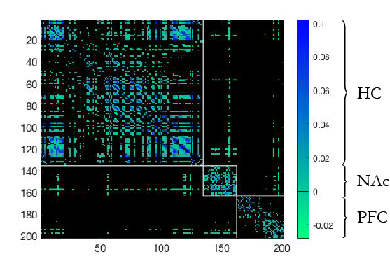
In a percolation problem one monitors the size of (fraction of nodes belonging to) the giant connected component $G_{\rm bond}$ as a function of the driving external parameter. In the present case, we first apply the graphical lasso for a given $\lambda$ and obtain the inferred matrix $J_{ij}$ from $C_{ij}$. We binarize this matrix and construct a network by considering a link if $|J_{ij}|$ is above a given small resolution threshold, as it is customary in the graphical lasso algorithm. We then monitor the giant component of this network for a given $\lambda$ versus the penalty parameter $\lambda$ and we search for the appearance of the giant component as $\lambda$ is decreased from a large value. The process of constructing the network by decreasing $\lambda$ adds links to an initially empty network as in bond percolation. We fix the penalty parameter $\lambda$, which tunes the sparsity of the network, as the highest value at which the giant component of the network appears between each cluster, in turn. i.e. such that all nodes in the three clusters HC-PFC-NAc are connected through a path. In other words, the final network is the sparsest architecture that yet has one connected giant component which includes nodes from the three clusters. The connectivity matrix is obtained by binarizing the obtained $J_{ij}$ from the graphical lasso at a given $\lambda$ by considering a link when $J_{ij}$ is non-zero with a given small resolution. The resulting connectivity matrix from $J_{ij}$ is shown in Supplementary Fig. 2, for the same representative animal used in Fig. 1g and 1j. From this matrix we identify the three anatomical components HC, PFC and NAc and the links inside the clusters or strong or intra-links and the links across the clusters, the weak or inter-links gallos .

Supplementary Figure 3: Size of the giant connected component $G$ as a function of the fraction of inactivated nodes, $q$ for all six rats for degree, CI, KC, EC, BC, and CC. For CI, smaller number of inactivated nodes are required to disintegrate the network consistently for all six rats.

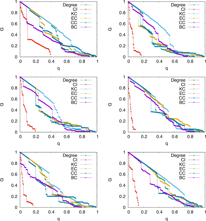
4 Measure of average maps of centralities in the brain network

For all nodes in the brain network we compute the score of each centrality for each experimental animal. We then rank all the nodes from high to low score. We then ’attack’ the brain network following each ranking for each centrality from hubs, CI, KC, EC, CC and BC. We monitor the size of the giant component as we remove a fraction of influential nodes $q$ following each strategy and for each network corresponding to each of the six animals mm ; morone2 . Supplementary Figure 3 shows the results. We see how the strategy following CI destroys the giant component with the smallest number of nodes. For each strategy, we extract the set of most influential nodes, the essential nodes according to each strategy, by considering the first nodes that reduce the size of the connected component to 5% of its original size. These are the set of essential nodes for each centrality and correspond to the ranking of top nodes according to each centrality.

Lastly, we normalize the ranking of each node using the following formula morone2 to compare across strategies:

$$R(i)=\frac{r_{o}-r_{i}}{r_{o}-1},$$ (8)

where $r_{i}$ is the ranking of node $i$, that is defined as the step at which it is inactivated (for example, the first node to be inactivated is assigned $r_{i}=1$, the second $r_{i}=2$, and so on). The quantity $r_{o}$ is a baseline, which, in our analysis, we set as the ranking of the node for which the giant active component takes the value $G=0.05$. Note that $R(i)=1$ represents the highest node. On the other hand, if node $i$ is not targeted by an external inactivation, then we set $R(i)=0$. The normalization in Eq. (8) allows us to properly sum over all samples to get an averaged map of the most important nodes in the brain network which allows us to compare the impact of each centrality. The results are used to generate the the hub-map in Fig. 2g and the averaged CI map in Fig. 2h, as well as all the centrality maps shown in Fig. 3.

5 Influencers map for the resting state dynamics

In this section we present results regarding which nodes are responsible for integration during resting state dynamics, as discussed in Sec. 2. The analysis of the essential nodes for integration presented in the main text, indeed, is performed on brain networks stimulated by LTP induction which, in addition to the hippocampus, produces the activation of the prefrontal cortex and of the nucleus accumbens. In the PRE-LTP condition, stimulation of the hippocampus does not recruit activation of neither the PFC nor the NAc and therefore, the relevance of these latter areas for brain integration cannot be investigated. To clarify their role in the brain network, we analyze the fMRI signal of the resting state dynamics in a PRE-LTP condition.

Since we are interested in investigating the role of the HC, the PFC and the NAc during unperturbed brain dynamics, we take into consideration the same anatomical areas, i.e. same voxels, studied to analyze the LTP-induced network. This guarantees that nodes in the resulting brain networks are the same for both the LTP-induced and the resting-state network. What changes between the two cases are the BOLD signals and, therefore, the statistical dependences between these voxels, i.e. the wiring of the resulting architecture.

Supplementary Figure 4: Average ($n=6$) CI-map for the resting-state brain dynamics. The map shows the CI-score (Eq. (2)) of each voxel averaged over six animals for the case of unperturbed brain PRE-LTP induction. High CI-score voxels are not localized in a single brain areas but appears spread around and mostly located between the hippocampus and the prefrontal cortex.

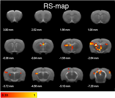
The analysis is done on the same six animals presented in the main text (in that case POST-LTP), same $p$-value ($p<0.001$). Each resting-state brain network is constructed similarly to the LTP-induced one, as described in Sec. 2 and in Supplementary Note 3. For each of these networks we rank the nodes according to the CI centrality measure, obtaining a CI-map for each rat. We then average the CI-score across the six animals, similarly to the LTP-induced networks, as described in Supplementary Note 4. The averaged results are shown in Supplementary Figure 4 which shows no role for the NAc as director of brain integration. High CI-score nodes, indeed, are less localized to a single brain area and are rather spread in different brain regions, mostly involving the hippocampus and the prefrontal cortex. These findings demonstrate that brain integration is related to brain dynamics. The role of the NAc as director of brain integration discussed in the main text is not simply arising because of its anatomical location in the brain but, rather, it is due to the functional re-organization stimulated by LTP-induction.

6 Directed brain network analysis

The network analysis of influencers in the rodent brain presented in Sec. 2 and 2 is based on the construction of an undirected network. All biological networks are directional and so is the neural wiring in the brain. At the neuronal level, indeed, each synapse and axon has a specific direction for the flow of electric and chemical signal. A single voxel, which is the maximal spatial resolution of a fMRI scan, contains about $10^{4}$ neurons. The information flow between two voxels can be thought as resulting from the average flow of chemical and electric signals between all the neurons in these voxels.

To date, Granger causality granger is a useful tool to statistically test probabilistic causal and directional relations between two temporal variables and since its introduction in 1969, it has been applied in several disciplines, ranging from finance to neuroscience and biology. In this section we re-construct the same brain networks induced by LTP for the rodent brain made of the active brain areas during fMRI scans, i.e. HC, NAc and PFC, as discussed in the main text and, in addition, we use Granger causality granger to infer probabilistic directions of the network’s links. We first start from the undirected network as discussed in Section 2 for each one of the six animals. For each connected pair of nodes in the functional network throughout an undirected link, we infer directionality of the connection by applying Granger causality to the BOLD signal of the pair of voxels. We use a confidence level $\alpha=0.01$ and a lapse $t_{l}=1$-step in the scanning time, which correspond to $2$ seconds, this is the minimum temporal resolution available from the fMRI in use.

Given two voxels $i$ and $j$, from their time series, we test the hypothesis $i$ Granger-causes $j$ and, if the hypothesis is accepted, we assign a link $i\to j$. We then test the opposite hypothesis: $j$ Granger-causes $i$. If both hypothesis are accepted we add no directionality to the link $i-j$, the same in the case when none of the two hypothesis is accepted. Therefore, directionality is assigned when either $i$ Granger-causes $j$ ($i\to j$) or $j$ Granger-causes $i$ ($j\to i$).

To find which are the influencers, i.e. the integrators, in this directional network we develop an heuristic version of the Collective Influence (CI) algorithm, presented in Eq. (2) in the SI, which accounts for link directionality. Once the network is directed, each node has a given in-degree ($k_{i}^{\rm{in}}$) and out-degree ($k_{i}^{\rm{out}}$) and undirected links contribute to both of them. A natural generalization of the CI algorithm to the directed case is then the following:

$${\rm CI^{\rm{DIR}}}_{\ell}(i)=(k_{i}^{*}-1)\sum_{j\in\partial{\rm Ball^{*}}(i,\ell)}(k_{j}^{*}-1)+\sum_{\begin{subarray}{c}j\in\mathcal{F}^{*}(i)\ :\\ k_{j}^{*\rm in-inter}\ =1\end{subarray}}(k_{j}^{*}-1)\sum_{m\in\partial{\rm Ball^{*}}(j,\ell)}(k_{m}^{*}-1).$$ (9)

Where here, slightly differently from the undirected case, $k_{i}^{*}=k_{i}^{\rm{in}}+k_{i}^{\rm{out}}$ is the total degree of node $i$, with $k_{i}^{\rm{in}}\equiv k_{i}^{\rm{in-intra}}+k_{i}^{\rm{in-inter}}$ that accounts for: the total in-links coming from nodes in the same network as $i$ ($k_{i}^{\rm in-intra}$); and in-links coming from nodes belonging to a different network than $i$ ($k_{i}^{\rm in-inter}$). Analogously, $k_{i}^{\rm{out}}\equiv\ k_{i}^{\rm out-intra}+k_{i}^{\rm out-inter}$, with $k_{i}^{\rm out-intra}$ and $k_{i}^{\rm out-inter}$ having a similar meaning but for the out-degree of node $i$. Diversely from Eq. (2), the symbol $\partial{\rm Ball^{*}}(i,\ell)$ indicates the directed sphere of influence of node $i$: this is the sphere of influence that can be reached with a directed path starting at node $i$. Whereas $j\in\mathcal{F}^{*}(i):k_{j}^{*\rm in-inter}\ =1$ instead indicates the set of nodes connected to $i$ through a directed interlink and which have no more interlinks with any of the other nodes in the network.

Supplementary Figure 5: Average ($n=6$) CI-directed map. The map indicates the CI-score (Eq. (9)) of each voxel averaged over six animals for the case of directed brain network. The Nucleus Accumbens appears as the area with the highest CI averaged score and, therefore, it is identified as the main area responsible for integration.

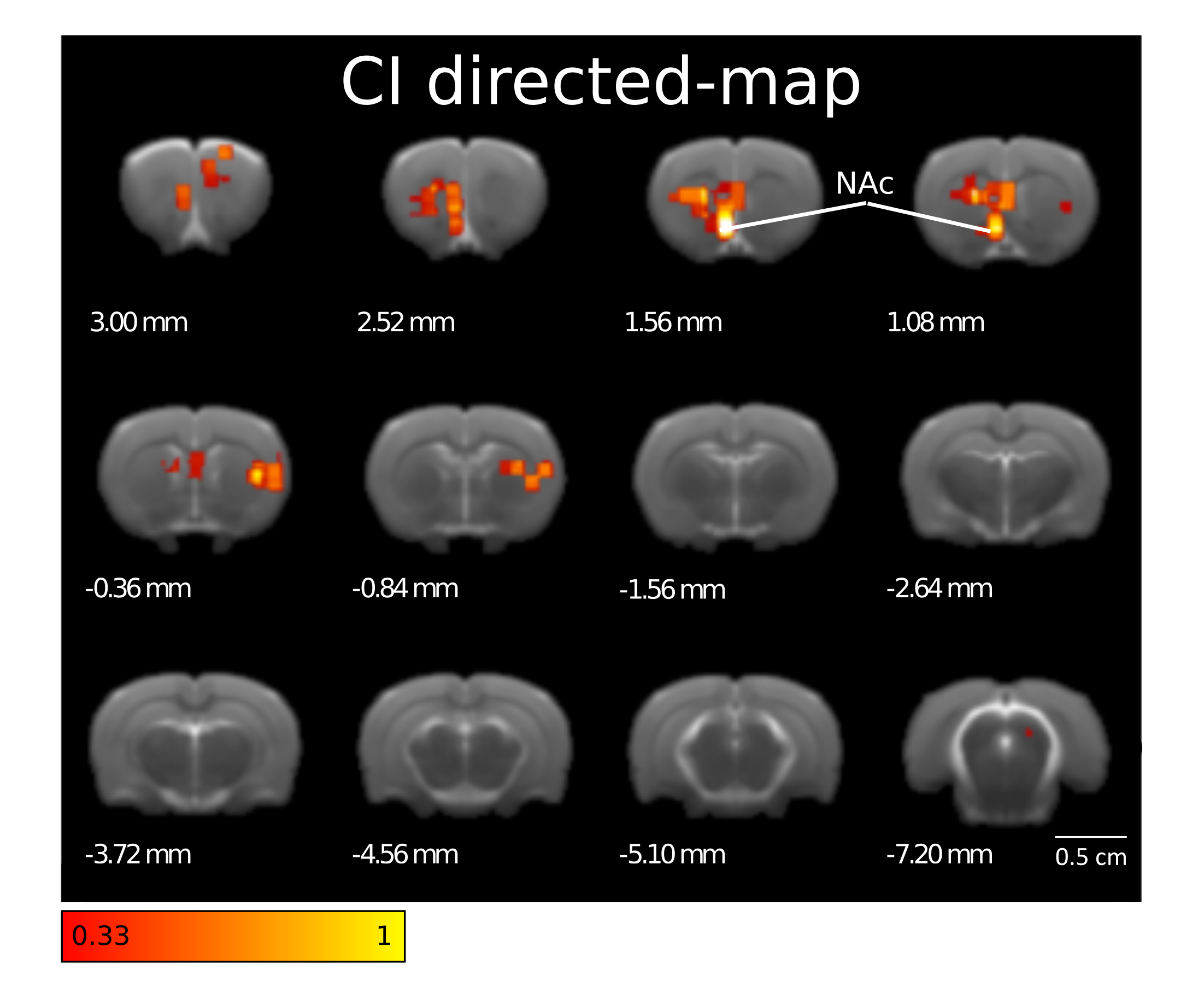
To identify the influencers of the directed brain network, for each rat, we compute the directed CI-score according to Eq. (9), in analogy with the undirected case, for each node in the brain network. For each animal, we then rank the nodes from high to low score and we then compute an average CI-directed map similarly to what described in Supplementary Note 4. Results are shown in Supplementary Fig. 5, to be compared with results for the undirected network discussed in the main text and illustrated in Fig. 2h. Despite the fact that the networks are directed in this case, the nucleus accumbens still results to be the brain area with the highest CI-directed score and so, according to our theory, the main brain areas responsible for integration.

7 Degree analysis of nodes responsible for integration

Supplementary Figure 6: Degree distribution across animals ($n=6$) of: (blue bins) the whole brain network; (green bins) top 30 CI nodes; (red bins) top 30 hub nodes. The figure shows that the top CI nodes, which our theory identify as responsible for brain integration, are comparatively of lower degree than hub nodes in the same networks.

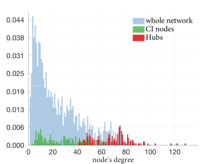
In this section we present a study of the degree statistics for the top CI nodes in each rodent brain network and of the top hub nodes in the same network. In particular, for each rat brain network, we identify the top 30 CI nodes according to equation (2) and we then determine the degree of each one of these nodes in their relative network. Analogously, for each rat, we also identify the top 30 hub nodes by using a high-degree algorithm and then determine their degree. We choose the first 30 nodes because, across animals, this is the max number of CI nodes which can be removed before the network is completely dismantled and so, the max number of nodes which can be used to compare the CI and hub degree statistics. For completeness, we also compute the degree statistics of all rodent brain networks by identifying the degree of each node in the network. In Supplementary Fig. 6 we report the corresponding degree distributions obtained from the above analyses. This figure illustrates that high CI nodes, i.e. nodes that we find responsible for integration within our theory, are comparatively of lower degree than hubs in the brain network.

8 Pharmacogenetic (Dreadd) experiment

The fundamental goal of this experiment is to use Designer Receptors Exclusively Activated by Designer Drugs (DREADDs) technology armbruster ; roth2016 to specifically inactivate nodes in the shell part of the nucleus accumbens (NAc), the contralateral hippocampus (cHC), the anterior part of the prefrontal cortex (PFC), and the somatosensory cortex (S1) and study, using fMRI and optimal percolation analysis, its impact on the functional architecture in the memory network induced by LTP. More specifically, with the aid of adenoviral vectors, we directed the expression of a Gi-DREADD (hM4Di) protein into the target regions which, under intra-peritoneal administration of the otherwise inert ligand clozapine-N-oxide (CNO), activates the receptor inducing neuronal silencing and blocking those regions output. Details are provided below.

Subjects

A total of 15 Sprague-Dawley male rats, weighing between 260-280 g, were used in this experiment. From these, three animals were not considered in the analysis due to absence or poor DREADD expression in the post-mortem validation. As before, animals were purchased from Janvier Labs (France) and maintained under a 12/12 h light/dark cycle (lights on 07:00-19:00 h) at room temperature (22$\pm$2 C). Food and water were provided ad libitum. Rats were housed in groups (4 animals per cage) and adapted to these conditions for at least 7 days before any manipulation.

Viral constructs and injection procedures

A mixture of two viruses is used to express hM4Di in the NAc. The first virus (AAV5-hSyn-GFP-Cre) drives the expression of Cre under the control of Synapsin (hSyn) in neurons and provides amplification of the Cre-dependent DREADD construct. The second virus (AAV5-hSyn-DIO-hM4D(Gi)-mCherry) expresses the inhibitory DREADD in Cre positive neurons. Both viruses are mixed 1:1 and 0.25 $\mu$L are injected stereotaxically in the shell portion of the NAc. For this, isoflurane anesthetized animals (4 $\%$ induction and 2.5 $\%$ for maintenance in 0.8 L/min $O_{2}$) are fixed in an stereotaxic frame, as described above, and bilateral craniotomies opened over the NAc (from bregma, AP 2.5 mm, ML 1.3 mm, and DV 7 mm), the PFC (from bregma AP -3.2 mm, ML 0.5 mm, and DV 2.0 and 3.8 mm), the contralateral Hippocampus (from bregma, AP -3.5 mm, ML 2.6 mm, and DV 3.2 mm), and the somatosensory cortex S1 (from bregma, AP 0.8 mm, ML 3.6 mm, and DV 1.4 mm). Injections are performed using silica cannula (GC22-20, 22 gauge internal cannula, WPI, USA) coupled to an infusion pump (SP200IZ Syringe pump, WPI, USA) through polyethylene tubing. The cannula is lowered slowly in the tissue to the final stereotaxic coordinate, stays in place 10 min before infusion starts, and 10 min more before retraction. Retraction is done slowly to prevent sucking the injected solution. At the end of the procedure, both craniotomies are covered with small amounts of bone cement (Palacos, Heraheus Medical GmbH, Germany), and the skin sutured. After the surgery animals receive analgesics (buprenorphine 0.3 mg, Buprex, Reckitt Benckiser Healthcare, UK) and antibiotics (enrofloxacine 3 $\%$, Syvaquinol 25, Syva, Spain) during 3-5 days.

DREADD fMRI procedures

We wait 4 to 6 weeks after the injection of the viruses to allow proper expression of the DREADD proteins in the NAc neurons. The experimental procedures for electrode implantation and fMRI data acquisition are the same as explained above for the LTP experiment. In addition, animals in this experiment are intraperitoneally cannulated for CNO administration inside the magnet. After baseline fMRI acquisition is completed (corresponding to the PRE-LTP, PRE-CNO condition), CNO is administered i.p (1 mg/Kg, 10 mL/Kg) and 30 min later a first set of functional images is acquired during low frequency stimulation (PRE-LTP, POST-CNO condition). After that, and still under the effect of CNO (which last more than 10 h, alexander ), LTP is induced as before and 1h later a new set of functional images is acquired (POST-LTP, POST-CNO condition).

Histology

At the end of each experiment, rats are perfused intracardially with 100 mL of 1$\%$ phosphate-buffered saline (PBS) solution and 100 mL of ice-cold 4$\%$ paraformaldehyde (PFA). Brains are kept for 24h on 4$\%$ PFA post-fixation at 4 C and cut in a fixed material vibratome in 50 $\mu$m thick slices. Slices are then stained with 4’,6-diamidino-2-phenylindole (DAPI) for photography under a fluorescence microscope. Expression of hM4Di in the NAc is validated by GFP fluorescence in the neurons.

9 Pharmacologic (TTX) inactivation experiments

In this experiment, we used an acute infusion of the voltage-dependent sodium channel blocker Tetrodotoxin (TTX), to strongly inactivate nodes in targeted regions and study, using fMRI and optimal percolation analysis, its impact on the functional architecture in the memory brain network induced by LTP.

Subjects

A total of 8 Sprague-Dawley male rats, weighing between 250-300 g, were used in this experiment, 4 for Hippocampal inactivation and 3 for S1 inactivation. As before, animals were purchased from Janvier Labs (France) and maintained under a 12/12 h light/dark cycle (lights on 07:00-19:00 h) at room temperature ($22\pm 2$ C). Food and water were provided ad libitum. Rats were housed in groups (4 animals per cage) and adapted to these conditions for at least 7 days before any manipulation.

Drug and injection procedures

Urethane anesthetized animals are fixed in a stereotaxic frame, as described above, and craniotomies are opened bilaterally over the Hippocampus (from bregma, AP -3.5 mm, ML 2.6 mm, and DV 3.2 mm), or the somatosensory cortex S1 (from bregma, AP 0.8 mm, ML 3.6 mm, and DV 1.4 mm). Injections are performed using silica cannula (GC22-20, 22-gauge internal cannula, WPI, USA) coupled to an infusion pump (SP200IZ Syringe pump, WPI, USA) through polyethylene tubing. The cannula is lowered slowly in the tissue to the final stereotaxic coordinate, stays in place 10 min before infusion starts, and 10 min more before retraction. $0,5\mu$L of TTX (100 $\mu$M in ACSF) are infused in the target region. Retraction is done slowly to prevent sucking the injected solution. Two multichannel recording electrodes are inserted in the ipsilateral and contralateral Hippocampus to account for the induced TTX inactivation and the successful induction of LTP. After TTX is infused as described above, field potentials in the contralateral Hippocampus are abolished, whilst field potentials in the ipsilateral Hippocampus remain intact (not shown). After that, LTP induction and fMRI procedures proceed as described in the main text and Supplementary Note 2.

Supplementary References

Kitsak, M., Gallos, L. K., Havlin, S., Liljeros, F., Muchnik, L., Stanley, H. E. & Makse, H. A., Identification of influential spreaders in complex networks, Nature Phys., 6, 888-893, (2010).

Hagmann, P., Cammoun, L., Gigandet, X., Meuli, R., Honey, C. J., Wedeen, V. J. and Sporns, O., Mapping the structural core of human cerebral cortex, PLoS Biol, 6, e159, (2008).

Seidman, S. B., Network structure and minimum degree. Soc. Networks 5, 269-287, (1983).

Morone, F. & Makse, H. A., Influence maximization in complex networks through optimal percolation, Nature, 524, 65-68, (2015).

Morone, F., Roth, K., Min, B., Stanley, H. E. & Makse, H. A., Model of brain activation predicts the neural collective influence map of the human brain, Proc. Natl Acad. Sci. USA, 114, 3849-3854, (2017).

McCulloch, W. & Pitts, W., A logical calculus of the ideas immanent in nervous activity, B. of Math. Biophys. 5, 115-133, (1943).

Hashimoto, K., Zeta functions of finite graphs and representations of p-adic groups. Adv. Stud. Pure Math., 15, 211-280, (1989).

Angel, O., Friedman, J. & Hoory, S., The non-backtracking spectrum of the universal cover of a graph, Trans. Amer. Math. Soc., 367, 4287-4318, (2015).

Newman, M. E. J., Networks: An Introduction, (Oxford University Press, Oxford, 2010).

Freeman, L. C., A set of measures of centrality based on betweenness, Sociometry, 40, 35-41, (1977).

Straffin, P. D., Linear algebra in geography: eigenvectors of networks, Mathematics Magazine, 53, 269-276, (1980).

Martin, T., Zhang, X. & Newman, M. E. J., Localization and centrality in networks, Phys. Rev. E, 90, 052808, (2014).

Bavelas, A., Communication patterns in tasks oriented groups, J. Acoust. Soc. Am., 22, 271-282, (1950).

Bliss, T. V. P., Collingridge, G. L. & Morris, R. in The Hippocampus book, Andersen, P., Morris, R., Amaral, R., Bliss, T. V. P. & O’Keefe, J. (Oxford University Press, Oxford, 2007).

Lynch, M. A., Long-term potentiation and memory, Physiol. Rev., 84, 87-136, (2004).

Bliss, T. V. & Lomo, T., Long-lasting potentiation of synaptic transmission in the dentate area of the anaesthetized rabbit following stimulation of the perforant path, J. Physiol, 232, 331-356, (1973).

Bliss, T. V. & Collingridge, G. L., A synaptic model of memory: long-term potentiation in the hippocampus, Nature, 361, 31-39, (1993).

Martin, S. J., Grimwood, P. D. & Morris, R. G. M., Synaptic plasticity and memory: An Evaluation of the Hypothesis, Annu. Rev. Neurosci., 23, 649-711, (2000).

Morris, R. G., Episodic-like memory in animals: psychological criteria, neural mechanisms and the value of episodic-like tasks to investigate animal models of neurodegenerative disease, Philos. Trans. R. Soc. Lond. B Biol. Sci., 356, 1453-1465, (2001).

Squire, L. R., Mechanisms of memory, Science, 232, 1612-1619, (1986).

Canals, S., Beyerlein, M., Merkle, H. & Logothetis, N. K., Functional MRI evidence for LTP-induced neural network reorganization, Curr. Bio., 19, 398-403, (2009).

Alvarez-Salvado, E., Pallares, V. G., Moreno, A. & Canals, S., Functional MRI of long-term potentiation: imaging network plasticity, Philos. Trans. R. Soc. Lond. B Biol. Sci., 369, 20130152, (2014).

Canals, S., Beyerlein, M., Murayama, Y. & Logothetis, N. K., Electric stimulation fMRI of the perforant pathway to the rat hippocampus, Magn. Reson. Imaging, 26, 978-986, (2008).

Canals, S., Beyerlein, M., Keller, A. L. Murayama, Y. & Logothetis, N. K. Magnetic resonance imaging of cortical connectivity in vivo, Neuroimage, 40, 458-472, (2008).

Jenkinson, M., Beckmann, C. F., Behrens, T. E., Woolrich, M. W. & Smith. S. M. FSL, Neuroimage, 62, 782-790, (2012).

Smith, S.M., Jenkinson, M., Woolrich, M.W., Beckmann, C.F., Behrens, T.E., Johansen-Berg, H., Bannister, P.R., De Luca, M., Drobnjak, I., Flitney, D.E. & Niazy, R.K., Advances in functional and structural MR image analysis and implementation as FSL, Neuroimage, 23, 208-219, (2004).

Cox, R. W., AFNI: software for analysis and visualization of functional magnetic resonance neuroimages, Comput. Biomed. Res., 29, 162-173, (1996).

Cox, R. W., AFNI: What a long strange trip it has been, Neuroimage, 62, 743-747, (2012).

Jenkinson, M., Bannister, P., Brady, M. & Smith, S., Improved optimization for the robust and accurate linear registration and motion correction of brain images, Neuroimage, 17, 825-841, (2002).

Smith, S. M., Fast robust automated brain extraction, Hum. Brain Mapp., 17, 143-155, (2002).

Schwarz, A.J., Danckaert, A., Reese, T., Gozzi, A., Paxinos, G., Watson, C., Merlo-Pich, E.V. & Bifone, A., A stereotaxic MRI template set for the rat brain with tissue class distribution maps and co-registered anatomical atlas: application to pharmacological MRI., Neuroimage, 32, 538-550, (2006).

Jenkinson, M. & Smith, S. A global optimisation method for robust affine registration of brain images, Med. Image Anal., 5, 143-156, (2001).

Paxinos, G. & Watson, C. The Rat Brain in Stereotaxic Coordinates, (Academic Press, New York, 2007).

Park, H. J. & Friston, K., Structural and functional brain networks: from connections to cognition, Science, 342, 6158, (2013).

Robinson, P. A., Sarkar, S., Pandejee, G. M. & Henderson, J. A., Determination of effective brain connectivity from functional connectivity with application to resting state connectivities, Phys. Rev. E, 90, 012707, (2014).

Deco, G. McIntosh, A. R., Shen, K., Hutchison, R. M., Menon, R. S., Everling, S., Hagmann, P. & Jirsa, V. K., Identification of optimal structural connectivity using functional connectivity and neural modeling, J. Neurosci., 34, 7910-7916, (2014).

Robinson, P. A., Interrelating anatomical, effective, and functional brain connectivity using propagators and neural field theory, Phys. Rev. E, 85, 011912, (2012).

Sarkar, S., Chawla, S. & Xu, D., On inferring structural connectivity from brain functional-MRI data, arxiv.org/pdf/1502.06659, (2015).

Hespanha, J. P., An efficient MatLab algorithm for graph partitioning, University of California, 1-8, (2004).

Bullmore, E. & Sporns, O., Complex brain networks: graph theoretical analysis of structural and functional systems, Nature Rev. Neurosci., 10, 186-198, (2009).

Friedman, J., Hastie, T. & Tibshirani, R., Sparse inverse covariance estimation with the graphical lasso, Biostatistics, 9, 432-441, (2008).

Erdös, P. & Rényi, A., On the evolution of random graphs, Publ. Math. Inst. Hung. Acad. Sci, 5, 17-61, (1960).

Bollobás, B. & Riordan, O., Percolation, (Cambridge University Press, Cambridge, 2006).

Bollobás, B, Random Graphs, (Academic Press, London, 1985).

Stauffer, D. & Aharony, A. , Introduction To Percolation Theory: Revised (Taylor & Francis, ed. 2, 1994).

Gallos, L. K., Makse, H. A. & Sigman, M., A small world of weak ties provides optimal global integration of self-similar modules in functional brain networks, Proc. Natl. Acad. Sci. USA, 109, 2825-2830, (2012).

Granger, C. W. J., Investigating Causal Relations by Econometric Models and Cross-spectral Methods, Econometrica, 37, 424-438, (1969).

Roth, B. L., DREADDs for Neuroscientists. Neuron 17, 683-694, (2016).

Armbruster, B. N., Li, X., Pausch, M. H., Herlitze, S. & Roth, B. L., Evolving the lock to fit the key to create a family of G protein coupled receptors potently activated by an inert ligand, Proc. Natl. Acad. Sci. USA, 104, 5163-5168, (2007).

Alexander, G. M., Rogan, S. C., Abbas, A. I., Armbruster, B. N., Pei, Y., Allen, J. A., Nonneman, R. J., Hartmann, J., Moy, S. S., Nicolelis, M. A. & McNamara, J. O., Remote control of neuronal activity in transgenic mice expressing evolved G protein-coupled receptors, Neuron, 63, 27-39, (2009).

References

- (1) Dehaene, S. & Naccache, L., Towards a cognitive neuroscience of consciousness: basic evidence and a workspace framework, Cognition, 79, 1-37, (2001).
- (2) Sporns, O., Network attributes for segregation and integration in the human brain, Curr. Opin. Neurobiol., 23, 162-171, (2013).