UniverseMachine: The Correlation between Galaxy Growth and Dark Matter Halo Assembly from $z=0-10$

Abstract

We present a method to flexibly and self-consistently determine individual galaxies’ star formation rates (SFRs) from their host haloes’ potential well depths, assembly histories, and redshifts. The method is constrained by galaxies’ observed stellar mass functions, SFRs (specific and cosmic), quenched fractions, UV luminosity functions, UV–stellar mass relations, IRX–UV relations, auto- and cross-correlation functions (including quenched and star-forming subsamples), and quenching dependence on environment; each observable is reproduced over the full redshift range available, up to $0<z<10$. Key findings include: galaxy assembly correlates strongly with halo assembly; quenching correlates strongly with halo mass; quenched fractions at fixed halo mass decrease with increasing redshift; massive quenched galaxies reside in higher-mass haloes than star-forming galaxies at fixed galaxy mass; star-forming and quenched galaxies’ star formation histories at fixed mass differ most at $z<0.5$; satellites have large scatter in quenching timescales after infall, and have modestly higher quenched fractions than central galaxies; Planck cosmologies result in up to $0.3$ dex lower stellar—halo mass ratios at early times; and, nonetheless, stellar mass–halo mass ratios rise at $z>5$. Also presented are revised stellar mass—halo mass relations for all, quenched, star-forming, central, and satellite galaxies; the dependence of star formation histories on halo mass, stellar mass, and galaxy SSFR; quenched fractions and quenching timescale distributions for satellites; and predictions for higher-redshift galaxy correlation functions and weak lensing surface densities. The public data release (DR1) includes the massively parallel ($>10^{5}$ cores) implementation (the UniverseMachine), the newly compiled and remeasured observational data, derived galaxy formation constraints, and mock catalogues including lightcones.

1 Introduction

In $\Lambda$CDM cosmologies, galaxies form at the centres of gravitationally self-bound, virialized dark matter structures (known as haloes). Haloes form hierarchically, and the largest collapsed structure in a given overdensity (i.e., a central halo) can contain many smaller self-bound structures (satellite haloes). While the broad contours of galaxy formation physics are known (see Silk & Mamon, 2012; Somerville & Davé, 2015, for reviews), a fully predictive framework from first principles does not yet exist (see Naab & Ostriker, 2017, for a review).

Traditional theoretical methods include hydrodynamical and semi-analytic models, which use known physics as a strong prior on how galaxies may form. For example, current implementations attempt to simulate the effects of supernovae, radiation pressure, multiphase gas, black hole accretion, photo- and collisional ionization, and chemistry (see Somerville & Davé, 2015; Naab & Ostriker, 2017, for reviews). All such methods approximate physics below their respective resolution scales (galaxies for semi-analytic models; particles and/or grid elements for hydrodynamical simulations), and different reasonable approximations lead to different resulting galaxy properties (Lu et al., 2014b; Kim et al., 2016).

These methods are complemented by empirical modeling, wherein the priors are significantly weakened and the physical constraints come almost entirely from observations. Current empirical models constrain physics averaged over galaxy scales, similar to semi-analytical models. Indeed, as empirical modeling has grown in complexity and self-consistency, as well as in the number of galaxy (e.g., Moster et al., 2018; Rodríguez-Puebla et al., 2017; Somerville et al., 2018), gas (e.g., Popping et al., 2015), metallicity (e.g., Rodríguez-Puebla et al., 2016b), and dust (Imara et al., 2018) observables generated, the mechanics of semi-analytic and empirical models have become increasingly similar. For example, the techniques of post-processing merger trees from N-body simulations, comparing to galaxy correlation functions, and using orphan galaxies were commonplace in semi-analytical models well before they were used in empirical ones (Roukema et al., 1997; Kauffmann et al., 1999).

Nonetheless, the presence or absence of strong physical priors remains a key difference between empirical and semi-analytic models. While semi-analytic models can therefore obtain tighter parameter constraints for the same data (or lack thereof), empirical models can reveal physics that was not previously expected to exist (e.g., Behroozi et al., 2013c; Behroozi & Silk, 2015). In cases where traditional methods have strong disagreements (e.g., on the mechanism for galaxy quenching), this latter quality can be very powerful, and is hence a strong motivation for using empirical modeling here.

Most current empirical models relate galaxy properties to properties of their host dark matter haloes. Larger haloes host larger galaxies, with relatively tight scatter in the stellar mass—halo mass relation (More et al., 2009; Yang et al., 2009; Leauthaud et al., 2012; Reddick et al., 2013; Watson & Conroy, 2013; Tinker et al., 2013; Gu et al., 2016). Hence, it has become common to investigate average galaxy growth via a connection to the average growth of haloes (Zheng et al. 2007; White et al. 2007; Conroy & Wechsler 2009; Firmani & Avila-Reese 2010; Leitner 2012; Béthermin et al. 2013; Wang et al. 2013; Moster et al. 2013; Behroozi et al. 2013e, f; Mutch et al. 2013; Birrer et al. 2014; Marchesini et al. 2014; Lu et al. 2014a, 2015b; Papovich et al. 2015; Li et al. 2016; see Wechsler & Tinker 2018 for a review). These studies have found that the stellar mass—halo mass relation is relatively constant with redshift from $0<z<4$ (Behroozi et al., 2013c), but may evolve significantly at $z>4$ (Behroozi & Silk, 2015; Finkelstein et al., 2015b; Sun & Furlanetto, 2016).

If galaxy mass is tightly correlated with halo mass on average, it is natural to expect that individual galaxy assembly could be correlated with halo assembly. This assembly correlation for individual galaxies has strong observational support. For example, satellite galaxies in clusters have redder colours (implying lower star formation rates; SFRs) and more elliptical morphologies than similar-mass galaxies in the field (Hubble & Humason, 1931, and references thereto). At the same time, the satellite haloes hosting these satellite galaxies have undergone significant stripping due to cluster tidal forces (Tormen et al., 1998; Kravtsov et al., 2004; Knebe et al., 2006; Hahn et al., 2009; Wu et al., 2013; Behroozi et al., 2014a). Thus, there is a correlation between the assembly histories of satellite galaxies and satellite haloes, regardless of whether there is a direct causation.

For central galaxies (i.e., the main galaxies in central haloes), several studies (Tinker et al. 2012, Berti et al. 2017, Wang et al. 2018, and this study) have also found correlations between these galaxies’ quenched fractions (i.e., the fraction not forming stars) and the surrounding environment. At the same time, environmental density strongly correlates with halo accretion rates (Hahn et al., 2009; Behroozi et al., 2014a; Lee et al., 2017). This would again suggest a correlation (and again not necessarily causation) between central galaxies’ star formation rates and their host halo matter accretion rates.

Empirical models that correlate galaxy star formation rates or colours with halo concentrations (correlated with halo formation time; Wechsler et al. 2002) have shown success in matching galaxy autocorrelation functions, weak lensing, and radial profiles of quenched galaxy fractions around clusters (Hearin & Watson, 2013; Hearin et al., 2014; Watson et al., 2015). Models that relate galaxy SFRs linearly to halo mass accretion rates (albeit non-linearly to halo mass; Taghizadeh-Popp et al., 2015; Becker, 2015; Rodríguez-Puebla et al., 2016a; Sun & Furlanetto, 2016; Mitra et al., 2017; Cohn, 2017; Moster et al., 2018) have also shown success in this regard. To date, all such models have made a strong assumption that galaxy formation is perfectly correlated to a chosen proxy for halo assembly.

In our approach, we do not impose an a priori correlation between galaxy assembly and halo assembly. Instead, given that galaxy clustering depends strongly on this correlation, we can directly measure it. Our method first involves making a guess for how galaxy SFRs depend on host halo potential well depth, assembly history, and redshift. This ansatz is then self-consistently applied to halo merger trees from a dark matter simulation, resulting in a mock universe; this mock universe is compared directly with real observations to compute a Bayesian likelihood. A Markov Chain Monte Carlo algorithm then makes a new guess for the galaxy SFR function, and the process is repeated until the range of SFR functions that are compatible with observations is fully sampled.

Observational constraints used here include stellar mass functions, UV luminosity functions, the UV–stellar mass relation, specific and cosmic SFRs, galaxy quenched fractions, galaxy autocorrelation functions, and the quenched fraction of central galaxies as a function of environmental density. We also compare to galaxy-galaxy weak lensing. High-redshift constraints have improved dramatically in the past five years due to the CANDELS, 3D-HST, ULTRAVISTA, and ZFOURGE surveys (Grogin et al., 2011; Brammer et al., 2012; McCracken et al., 2012). At the same time, pipeline and fitting improvements have made significant changes to the inferred stellar masses of massive low-redshift galaxies (Bernardi et al., 2013). As with past analyses (Behroozi et al., 2010, 2013e), we marginalize over many systematic uncertainties, including those from stellar population synthesis, dust, and star formation history models.

We present the simulations and the new compilation of observational data in §2, followed by the methodology in §3. The main results, discussion, and conclusions are presented in §4, §5, and §6, respectively. Appendices discuss alternate parametrizations for halo assembly history (A), the need for orphan satellites (B), the compilation of and uncertainties in the observational data (C), revised fits to UV–stellar mass relations (D), the functional forms used (E), code parallelization and performance (F), results for non-universal stellar initial mass functions (G), the best-fitting model and 68% parameter confidence intervals (H), parameter correlations (I), and fits to stellar mass–halo mass relations (J).

For conversions from luminosities to stellar masses, we assume the Chabrier (2003) stellar initial mass function, the Bruzual & Charlot (2003) stellar population synthesis model, and the Calzetti et al. (2000) dust law. We adopt a flat, $\Lambda$CDM cosmology with parameters ($\Omega_{m}=0.307$, $\Omega_{\Lambda}=0.693$, $h=0.678$, $\sigma_{8}=0.823$, $n_{s}=0.96$) consistent with Planck results (Planck Collaboration et al., 2016). Halo masses follow the Bryan & Norman (1998) spherical overdensity definition and refer to peak historical halo masses extracted from the merger tree ($M_{\mathrm{peak}}$) except where otherwise specified.

2 Simulations & Observations

Table 1: Summary of Observational Constraints

Type	Redshifts	Primarily Constrains	Details & References
Stellar mass functions∗	$0-4$	SFR$-v_{\mathrm{Mpeak}}$ relation	Appendix C.2
Cosmic star formation rates∗	$0-10$	SFR$-v_{\mathrm{Mpeak}}$ relation	Appendix C.3
Specific star formation rates∗	$0-8$	SFR$-v_{\mathrm{Mpeak}}$ relation	Appendices C.3, C.4
UV luminosity functions	$4-10$	SFR$-v_{\mathrm{Mpeak}}$ relation	Appendix C.5
Quenched fractions∗	$0-4$	Quenching$-v_{\mathrm{Mpeak}}$ relation	Appendix C.6
Autocorrelation functions for quenched/SF/all galaxies from SDSS†	$\sim 0$	Quenching/assembly history correlation	Appendix C.7
Cross-correlation functions for galaxies from SDSS†	$\sim 0$	Satellite disruption	Appendix C.7
Autocorrelation functions for quenched/SF galaxies from PRIMUS∗	$\sim 0.5$	Quenching/assembly history correlation	Appendix C.7
Quenched fraction of primary galaxies as a function of neighbour density${\dagger}$	$\sim 0$	Quenching/assembly history correlation	Appendix C.8
Median UV–stellar mass relations${\dagger}$	$4-8$	Systematic Stellar Mass Biases	Appendix D
IRX–UV relations	$4-7$	Dust	Appendix D

Notes. SDSS: the Sloan Digital Sky Survey. PRIMUS: the PRIsm MUlti-object Survey. $v_{\mathrm{Mpeak}}$: $v_{\mathrm{max}}$ at the time of peak historical halo mass.

^∗: renormalized/converted in this study to more uniform modeling assumptions. ${\dagger}$: newly measured or reanalyzed in this study.

2.1 Simulations

We use the Bolshoi-Planck dark matter simulation (Klypin et al., 2016; Rodríguez-Puebla et al., 2016b) for halo properties and assembly histories. Bolshoi-Planck follows a periodic, comoving volume 250 $h^{-1}$ Mpc on a side with 2048³ particles ($\sim 8\times 10^{9}$), and was run with the art code (Kravtsov et al., 1997; Kravtsov & Klypin, 1999). The simulation has high mass ($1.6\times 10^{8}h^{-1}\;\mathrm{M}_{\odot}$), force (1 $h^{-1}$ kpc), and time output (180 snapshots spaced equally in $\log(a)$) resolution. The adopted cosmology (flat $\Lambda$CDM; $h=0.678$, $\Omega_{m}=0.307$, $\sigma_{8}=0.823$, $n_{s}=0.96$) is compatible with Planck15 results (Planck Collaboration et al., 2016). We also use the MDPL2 dark matter simulation (Klypin et al., 2016; Rodríguez-Puebla et al., 2016b) to calculate covariance matrices for auto- and cross-correlation functions. MDPL2 adopts an identical cosmology to Bolshoi-Planck, except for assuming $\sigma_{8}=0.829$, and follows a 1 $h^{-3}$ Gpc³ region with 3840³ particles ($\sim 57\times 10^{9}$). The mass ($2.2\times 10^{9}\;\mathrm{M}_{\odot}$) and force (5 $h^{-1}$ kpc) resolution are coarser than for Bolshoi-Planck. For both simulations, halo finding and merger tree construction used the rockstar (Behroozi et al., 2013b) and Consistent Trees (Behroozi et al., 2013d) codes, respectively.

2.2 Observations

As summarized in Table 1, we combine recent constraints from stellar mass functions (SMFs; Table 5), cosmic star formation rates (CSFRs; Table 6), specific star formation rates (SSFRs; Table 7), quenched fractions (QFs), UV luminosity functions (UVLFs), UV–stellar mass relations (UVSM relations), and infrared excess–UV relations (IRX–UV relations) with measurements of galaxy auto- and cross-correlation functions (CFs) and the environmental dependence of central galaxy quenching. Full details are presented in Appendices C and D.

Briefly, stellar mass function (SMF) constraints include data from the Sloan Digital Sky Survey (SDSS), the PRIsm MUlti-object Survey (PRIMUS), UltraVISTA, the Cosmic Assembly Near-infrared Deep Extragalactic Legacy Survey (CANDELS), and the FourStar Galaxy Evolution Survey (ZFOURGE). These constraints cover $0<z<4$ and were renormalized as necessary to ensure consistent modeling assumptions (Table 4) and photometry for massive galaxies (Fig. 41). As noted in Kravtsov et al. (2018), improved photometry for massive galaxies significantly increases their stellar mass to halo mass ratios as compared to Behroozi et al. (2013e). In addition, based on null findings in Williams et al. (2016), there was no need to perform surface brightness corrections for low-mass galaxies as in Behroozi et al. (2013e).

Specific SFRs and cosmic SFRs cover $0<z<10.5$ and were only renormalized to a Chabrier (2003) initial mass function, as matching other modeling assumptions does not increase self-consistency between SFRs and the growth of SMFs (Madau & Dickinson, 2014; Leja et al., 2015; Tomczak et al., 2016). These data are taken from a wide range of surveys (including SDSS, GAMA, ULTRAVISTA, CANDELS, ZFOURGE) and techniques (including UV, $24\mu$m, radio, H$\alpha$, and SED fitting).

Quenched fractions as a function of stellar mass, from Bauer et al. (2013), Moustakas et al. (2013), and Muzzin et al. (2013), cover the range $0<z<3.5$. As discussed in Appendix C.6, these papers use different definitions for “quenched” (cuts in SSFR and UVJ luminosities, respectively), which we self-consistently model when comparing to each paper’s results. Stellar masses were renormalized as for SMFs.

Autocorrelation functions for all, quenched, and star-forming galaxies are newly measured from the SDSS (Appendix C.7), with covariance matrices measured from identical sky masks in mock catalogues of significantly greater volume. Cross-correlation functions of massive galaxies ($M_{\ast}>10^{11}\;\mathrm{M}_{\odot}$) with Milky-Way mass galaxies ($M_{\ast}\sim 10^{10.4}\;\mathrm{M}_{\odot}$) are also newly measured from the SDSS to help constrain satellite disruption. At $z\sim 0.5$, we use the correlation functions for quenched and star-forming galaxies from PRIMUS (Coil et al., 2017). As with the SDSS, covariance matrices are measured from mock catalogues; redshift errors are remeasured from a cross-comparison between the G10/COSMOS redshift catalogue (Davies et al., 2015) and the PRIMUS DR1 catalogue (Coil et al., 2011).

Correlation functions are primarily sensitive to satellite quenching, so constraining central galaxy quenching requires a different measurement. Here, we use the quenched fraction for primary galaxies (i.e., those that are the largest in a given surrounding volume) as a function of the number counts of lower-mass neighbours (Appendix C.8; see also Berti et al., 2017). This signal is significantly stronger and more robustly measurable than two-halo galactic conformity, and is a plausible cause thereof (Hearin et al., 2016). In addition, Lee et al. (2017) has shown that halo mass accretion rates correlate strongly with environmental density for central haloes, so this statistic helps constrain the correlation between halo mass and galaxy assembly for central haloes.

Finally, existing stellar mass functions at $z>4$ often depend on uncertain UV–stellar mass conversions, which results in significant interpublication scatter even on the same underlying data sets (e.g., Fig. 6 in Moster et al., 2018). We explore the underlying reason for these uncertainties in Appendix D, finding that uncertainties in the SED for star formation history and dust can be reduced by combining additional observables. As a result, we develop a new SED-fitting tool (SEDition; Appendix D) and use it to remeasure median UV–stellar mass relations from the Song et al. (2016) SED stacks for $z=4-8$ galaxies, combined with star formation history constraints from UV luminosity functions’ evolution and dust constraints from ALMA (Bouwens et al., 2016b). The resulting UV–stellar mass relations, combined with UV luminosity functions from Finkelstein et al. (2015a) and Bouwens et al. (2016a), replace constraints on SMFs at $z>4$.

3 Methodology

We summarize our approach in §3.1, followed by details for the SFR parameterization (§3.2), galaxy mergers (§3.3), stellar masses and luminosities (§3.4), and observational systematics including dust (§3.5).

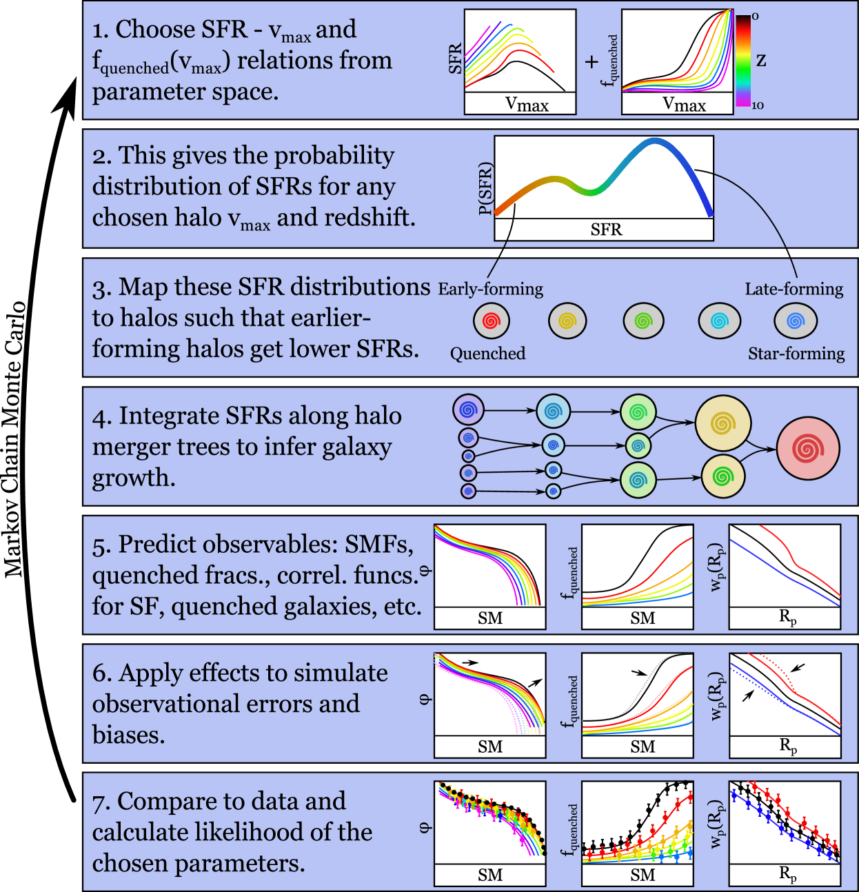
Figure 1: Visual summary of the method for linking galaxy growth to halo growth (§3).

Table 2: Table of parameters.

Symbol	Description	Equation	Parameters	Section
$\sigma_{\mathrm{SF}}(z)$	Scatter in SFR for star-forming galaxies	3	2	3.2
$V(z)$	Characteristic $v_{\mathrm{Mpeak}}$ in SFR – $v_{\mathrm{Mpeak}}$ relation	6	4	3.2
$\epsilon(z)$	Characteristic SFR in SFR – $v_{\mathrm{Mpeak}}$ relation	7	4	3.2
$\alpha(z)$	Faint-end slope of SFR – $v_{\mathrm{Mpeak}}$ relation	8	4	3.2
$\beta(z)$	Massive-end slope of SFR – $v_{\mathrm{Mpeak}}$ relation	9	3	3.2
$\gamma(z)$	Strength of Gaussian efficiency boost in SFR – $v_{\mathrm{Mpeak}}$ relation	10	3	3.2
$\delta$	Width of Gaussian efficiency boost in SFR – $v_{\mathrm{Mpeak}}$ relation	11	1	3.2
$Q_{\mathrm{min}}(z)$	Minimum quenched fraction	13	2	3.2
$V_{Q}(z)$	Characteristic $v_{\mathrm{Mpeak}}$ for quenching	14	3	3.2
$\sigma_{VQ}(z)$	Characteristic $v_{\mathrm{Mpeak}}$ width over which quenching happens	15	3	3.2
$r_{c}(z)$	Rank correlation between halo assembly history ($\Delta v_{\mathrm{max}}$) and SFR	16	4	3.2
$\tau_{R}(z)$	Correlation time for long-timescale random contributions to SFR rank	$-$	0	3.2
$f_{\mathrm{short}}$	Fraction of short-timescale random contributions to SFR rank	19	1	3.2
$T_{\mathrm{merge}}$	Threshold for $v_{\mathrm{max}}/v_{\mathrm{Mpeak}}$ at which disrupted haloes are no longer tracked	$-$	2	3.3
$f_{\mathrm{merge}}$	Fraction of host halo’s radius below which disrupted satellites merge into the central galaxy	$-$	1	3.3
$\alpha_{\mathrm{dust}}$	Characteristic rate at which dust increases with UV luminosity	23	1	3.4
$M_{\mathrm{dust}}(z)$	Characteristic UV luminosity for dust to become important	24	2	3.4
$\mu(z)$	Systematic offset in both observed stellar masses and SFRs	25	2	3.5
$\kappa(z)$	Additional systematic offset in observed SFRs	26	1	3.5
$\sigma_{\mathrm{SM,obs}}(z)$	Random error in recovering stellar masses	27	1	3.5
$\sigma_{\mathrm{SFR,obs}}(z)$	Random error in recovering SFRs	28	0	3.5

Notes. $v_{\mathrm{Mpeak}}$: $v_{\mathrm{max}}$ at the time of peak historical halo mass. $\Delta v_{\mathrm{max}}$ is described by Eq. 1 in §3.1. Symbols followed by “$(z)$” depend on redshift and are described by multiple parameters (see equation references above). $\tau_{R}$ is fixed to the halo dynamical time, $\left(\frac{4}{3}\pi G\rho_{\mathrm{vir}}\right)^{-1/2}$. The total number of free model parameters is 44.

Table 3: Table of priors.

Symbol	Description	Equation	Prior
$T_{\mathrm{orphan,300}}$	Threshold for $v_{\mathrm{max}}/v_{\mathrm{Mpeak}}$ at which disrupted haloes are no longer tracked around 300 km s-1 hosts	$-$	$U(0.2,1)$
$T_{\mathrm{orphan,1000}}$	Threshold for $v_{\mathrm{max}}/v_{\mathrm{Mpeak}}$ at which disrupted haloes are no longer tracked around 1000 km s-1 hosts	$-$	$U(0.2,1)$
$f_{\mathrm{merge}}$	Fraction of host halo’s virial radius below which disrupted satellites are merged with the central galaxy	$-$	$U(0,2)$
$\mu_{0}$	Value of $\mu$ at $z=0$, in dex	25	$G(0,0.14)$
$\mu_{a}$	Redshift scaling of $\mu$, in dex	25	$G(0,0.24)$
$\kappa$	Additional offset in observed vs. true SFR, in dex	26	$G(0,0.24)$
$\sigma_{\mathrm{SM,z}}$	Redshift scaling of $\sigma_{\mathrm{SM}}$	27	G(0.05, 0.015)

Notes. $G(x,y)$ is a Gaussian distribution with center $x$ and width $y$. $U(x,y)$ is a uniform distribution over $[x,y]$. Remaining parameters do not have explicit priors; $V$, $V_{Q}$, and $M_{D}$ are explored in logarithmic space, whereas the remainder are explored in linear space.

3.1 Design Overview

Our approach (Fig. 1) parametrizes galaxy SFRs as a function of halo potential well depth, redshift, and assembly history. For potential well depth, past works used peak historical halo mass (e.g., Moster et al., 2013; Behroozi et al., 2013e) or peak historical $v_{\mathrm{max}}$ (e.g., Reddick et al., 2013), where $v_{\mathrm{max}}$ is the maximum circular velocity of the halo ($\equiv\max(\sqrt{GM(<R)/R})$). Peak $v_{\mathrm{max}}$ better matches galaxy clustering (Reddick et al., 2013) and avoids pseudo-evolution issues (Diemer et al., 2013). Yet, strong, transient $v_{\mathrm{max}}$ peaks occur following major halo mergers (Behroozi et al., 2014a). Hence, we use the value of $v_{\mathrm{max}}$ at the redshift where the halo reached its peak mass ($v_{\mathrm{Mpeak}}\equiv v_{\mathrm{max}}(z_{\mathrm{M_{peak}}})$) so that transient peaks after mergers do not affect long-term SFRs.

Previous studies have varied SFRs with halo mass accretion rates (e.g., Becker, 2015; Rodríguez-Puebla et al., 2016a; Moster et al., 2018) and concentrations (Hearin & Watson, 2013; Watson et al., 2015). Satellites are problematic for both approaches, as neither satellite mass accretion nor concentration are robustly measured by halo finders (Onions et al., 2012; Behroozi et al., 2015b), and most solutions (e.g., using the time since accretion; Moster et al. 2018) cannot capture orbit-dependent effects.

Here, we use the $v_{\mathrm{max}}$ accretion history, which is robustly measurable for satellites (Onions et al., 2012) and yields more clearly orbit– and profile–dependent satellite SFRs. A rapid increase in $v_{\mathrm{max}}$ means both a large influx of gas and a better ability to retain existing gas, both of which would suggest higher SFRs. A rapid decrease implies either strong tidal stripping (as for satellites) or that the halo’s $v_{\mathrm{max}}$ peaked during a major merger and is now dropping rapidly (as for post-starburst galaxies), both suggesting lower SFRs. However, recent changes in $v_{\mathrm{max}}$ likely matter less for extremely stripped satellites—which we would expect to remain quenched. Hence, we adopt the following $v_{\mathrm{max}}$ history parameter:

$$\Delta v_{\mathrm{max}}\equiv\frac{v_{\mathrm{max}}(z_{\mathrm{now}})}{v_{\mathrm{max}}(\max(z_{\mathrm{dyn}},z_{\mathrm{M_{peak}}}))},$$ (1)

where $z_{\mathrm{dyn}}(t)$ is the redshift a dynamical time ($\equiv(\frac{4}{3}\pi G\rho_{\mathrm{vir}})^{-\frac{1}{2}}$) ago and $\rho_{\mathrm{vir}}(t)$ is the virial overdensity according to Bryan & Norman (1998). For most haloes, $\Delta v_{\mathrm{max}}$ corresponds to the relative change in $v_{\mathrm{max}}$ over the past dynamical time. However, for extremely stripped satellites, $\Delta v_{\mathrm{max}}$ corresponds to the relative change in $v_{\mathrm{max}}$ since they last accreted mass, preventing them from resuming star formation.

$\Delta v_{\mathrm{max}}$ is not the only option for parameterizing halo assembly (see Appendix A for alternatives). However, as discussed above, there are physical reasons for it to correlate well with galaxy SFRs. As long as there is some correlation between $\Delta v_{\mathrm{max}}$ and galaxy SFRs (regardless of the underlying causation), our approach remains valid to determine the correlation strength.

Any choice for the function $SFR(v_{\mathrm{Mpeak}},z,\Delta v_{\mathrm{max}})$ (see §3.2 and Table 2 for our parametrization; see Table 3 for priors) fully determines galaxy SFRs in every halo at every redshift in a dark matter simulation (Fig. 1). For each halo, the galaxy stellar mass and UV luminosity are self-consistently calculated from star formation histories along the halo’s assembly and merger history. This results in a mock observable universe (including galaxy positions, redshifts, stellar masses, SFRs, and luminosities) that can be directly compared to the real Universe. We compute the likelihood for a given point in parameter space using galaxy stellar mass functions, specific SFRs, cosmic SFRs, quenched fractions, UV luminosity functions, UV–stellar mass relations, IRX–UV relations, auto-correlation functions (for all, star-forming, and quiescent galaxies), cross-correlation functions, and measurements of central galaxy quenching with environment (§2.2), using covariance matrices where available. The likelihood function ($\exp(-\chi^{2}/2)$) is processed through an MCMC algorithm (a hybrid of adaptive Metropolis and stretch-step MCMC algorithms; Haario et al. 2001; Goodman & Weare 2010), resulting in empirical constraints on how galaxy growth correlates with halo growth.

3.2 SFR Distribution

We parametrize SFRs in haloes as a function of $v_{\mathrm{Mpeak}}$ ($v_{\mathrm{max}}$ at the redshift of peak halo mass), $z$, and $\Delta v_{\mathrm{max}}$ (logarithmic growth in $v_{\mathrm{max}}$ over the past dynamical time), summarized in Table 2. At fixed $v_{\mathrm{Mpeak}}$ and $z$, we assume that the SFR distribution is the sum of two log-normal distributions, corresponding to a quenched population and a star-forming population:

$$P(SFR|v_{\mathrm{Mpeak}},z)=f_{\mathrm{Q}}G(SFR_{\mathrm{Q}},\sigma_{\mathrm{Q}})+(1-f_{\mathrm{Q}})G(SFR_{\mathrm{SF}},\sigma_{\mathrm{SF}}),$$ (2)

where $G(\mu,\sigma)$ is a log-normal distribution with median $\mu$ and scatter $\sigma$; $f_{\mathrm{Q}}$ is the fraction of quenched galaxies, $SFR_{\mathrm{SF}}$ and $SFR_{\mathrm{Q}}$ are the median SFRs for star-forming and quenched galaxies, respectively, and $\sigma_{\mathrm{SF}}$ and $\sigma_{\mathrm{Q}}$ are the corresponding scatters.

All of these parameters ($f_{\mathrm{Q}},SFR_{\mathrm{Q}},SFR_{\mathrm{SF}},\sigma_{\mathrm{Q}},\sigma_{\mathrm{SF}}$) could vary with $v_{\mathrm{Mpeak}}$ and $z$. However, scatter in SFRs is not observed to vary with either stellar mass or redshift (Speagle et al., 2014), and the tight connection between stellar mass and halo mass (or $v_{\mathrm{max}}$) required to match galaxy clustering and weak lensing (Leauthaud et al., 2012; Tinker et al., 2013; Reddick et al., 2013) suggests that $\sigma_{\mathrm{SF}}$ need not vary much with $v_{\mathrm{Mpeak}}$ or $z$, either. However, we allow redshift flexibility to test this assumption, setting a maximum of 0.3 dex:

$$\sigma_{\mathrm{SF}}=\min(\sigma_{\mathrm{SF,0}}+(1-a)\sigma_{\mathrm{SF,1}},0.3)\;\mathrm{dex},$$ (3)

where $a$ is the scale factor. SFRs for quenched galaxies have large systematic uncertainties (Brinchmann et al., 2004; Salim et al., 2007; Wetzel et al., 2012; Hayward et al., 2014). As long as $SFR_{\mathrm{SF}}\gg SFR_{\mathrm{Q}}$, the exact value of $SFR_{\mathrm{Q}}$ does not impact galaxy stellar masses or colours. Hence, $SFR_{\mathrm{Q}}$ is set such that median specific SFRs for quenched galaxies are $10^{-11.8}$ yr^-1 and $\sigma_{\mathrm{Q}}$ is fixed at $0.36$ dex, matching SDSS values for $L^{*}$ galaxies (Behroozi et al., 2015a).

The functional form for $SFR_{\mathrm{SF}}(v_{\mathrm{Mpeak}},z)$ is based on the best-fitting $\langle SFR(M_{\mathrm{peak}},z)\rangle$ constraints from Behroozi et al. (2013e). We determined $M_{\mathrm{peak}}(v_{\mathrm{Mpeak}},z)$ (i.e., the median halo mass as a function of $v_{\mathrm{Mpeak}}$ and $z$) from the Bolshoi-Planck simulation (see §2.1), and find in Appendix E.2 that a double power law plus a Gaussian is a good fit to $\langle SFR_{\mathrm{SF}}(M_{\mathrm{peak}}(v_{\mathrm{Mpeak}},z),z)\rangle$. We hence adopt:

$$SFR_{\mathrm{SF}} = \epsilon\left[\left(v^{\alpha}+v^{\beta}\right)^{-1}+\gamma\exp\left(-\frac{\log_{10}(v)^{2}}{2\delta^{2}}\right)\right]$$ (4)

$$v = \frac{v_{\mathrm{Mpeak}}}{V\cdot\mathrm{km}\;\mathrm{s}^{-1}}$$ (5)

$$\log_{10}(V) = V_{0}+V_{a}(1-a)+V_{la}\ln(1+z)+V_{z}z$$ (6)

$$\log_{10}(\epsilon) = \epsilon_{0}+\epsilon_{a}(1-a)+\epsilon_{la}\ln(1+z)+\epsilon_{z}z$$ (7)

$$\alpha = \alpha_{0}+\alpha_{a}(1-a)+\alpha_{la}\ln(1+z)+\alpha_{z}z$$ (8)

$$\beta = \beta_{0}+\beta_{a}(1-a)+\beta_{z}z$$ (9)

$$\log_{10}(\gamma) = \gamma_{0}+\gamma_{a}(1-a)+\gamma_{z}z$$ (10)

$$\delta = \delta_{0}.$$ (11)

For the parameter redshift scaling (Eqs. 6–11), we generally follow Behroozi et al. (2013e) in having variables to control the parameter value at $z=0$, the scaling to intermediate redshift ($z\sim 1-2$), and the scaling to high redshift ($z>3$); we add one more parameter to decouple the moderately high redshift scaling ($z=3-7$) from the very high-redshift scaling ($z>7$). For $\beta$, we do not include this extra parameter, as the massive-end slope is ill-constrained at such high redshifts. The width of the Gaussian part of $SFR_{\mathrm{SF}}$ seems not to change significantly in fits to Behroozi et al. (2013e) constraints, so we keep $\delta$ fixed over the entire redshift range.

For the functional form for $f_{\mathrm{Q}}(v_{\mathrm{Mpeak}},z)$, we adopt:

$$f_{\mathrm{Q}} = Q_{\mathrm{min}}+(1.0-Q_{\mathrm{min}})\times$$ (12)

$$\left[0.5+0.5\mathrm{erf}\left(\frac{\log_{10}(\frac{v_{\mathrm{Mpeak}}}{V_{Q}\cdot\mathrm{km}\;\mathrm{s}^{-1}})}{\sqrt{2}\cdot\sigma_{VQ}}\right)\right],$$

where erf is the error function. This function smoothly rises from $Q_{\mathrm{min}}$ to 1 over a characteristic width $\sigma_{VQ}$, with the halfway point at the velocity $V_{Q}$. The adopted redshift scaling is:

$$Q_{\mathrm{min}} = \max(0,Q_{\mathrm{min,0}}+Q_{\mathrm{min,a}}(1-a))$$ (13)

$$\log_{10}(V_{Q}) = V_{Q,0}+V_{Q,a}(1-a)+V_{Q,z}z$$ (14)

$$\sigma_{VQ} = \sigma_{VQ,0}+\sigma_{VQ,a}(1-a)+\sigma_{VQ,la}\ln(1+z).$$ (15)

We verify that this functional form is sufficiently flexible to match observed quenched fractions in Appendix 53.

For haloes at a given $v_{\mathrm{Mpeak}}$ and $z$, the above parametrization determines the SFR distribution. In our approach, we assign higher SFRs to haloes with higher values of $\Delta v_{\mathrm{max}}$ (similar to the conditional abundance matching approach in Watson et al. 2015), allowing for random scatter in this assignment. Because satellites on average have much lower $\Delta v_{\mathrm{max}}$ values than centrals, zero scatter in the assignment would result in the largest quenched fractions for satellites. Increasing the scatter decreases the quenched fraction of satellites while increasing the quenched fraction of centrals. Observationally, this is strongly constrained by the ratio of autocorrelation strengths for quenched vs.  star-forming galaxies.

We let $r_{c}$ be the correlation coefficient between haloes’ rank orders in $\Delta v_{\mathrm{max}}$ and their rank orders in SFR (both at fixed $v_{\mathrm{Mpeak}}$ and $z$), and allow this correlation to depend on $v_{\mathrm{Mpeak}}$ and $z$:

$$r_{c}(v_{\mathrm{Mpeak}},z) = r_{\mathrm{min}}+(1.0-r_{\mathrm{min}})\times$$ (16)

$$\left[0.5-0.5\mathrm{erf}\left(\frac{\log_{10}\left(\frac{v_{\mathrm{Mpeak}}}{V_{R}\cdot\mathrm{km}\;\mathrm{s}^{-1}}\right)}{\sqrt{2}\cdot r_{\mathrm{width}}}\right)\right]$$

$$\log_{10}(V_{R}) = V_{R,0}+V_{R,a}(1-a).$$ (17)

Similar to the functional form for $f_{Q}$, this function declines smoothly from $1$ to $r_{\mathrm{min}}$, with a characteristic width $r_{\mathrm{width}}$ and the halfway point at the velocity $V_{R}$. We allow $r_{\mathrm{width}}$ to be negative, which would result in $r_{c}$ increasing (instead of declining) from $r_{\mathrm{min}}$ to $1$ with increasing $v_{\mathrm{Mpeak}}$. In principle, $r_{\mathrm{min}}$ and $r_{\mathrm{width}}$ could vary with redshift, but as we do not have enough $z>0$ autocorrelation data to constrain the redshift dependence of these parameters, we leave them fixed. A halo’s resulting (cumulative) percentile rank in the SFR distribution ($\equiv C_{\mathrm{SF}}$) is given by:

$$C_{\mathrm{SF}}=C\left(r_{c}\cdot C^{-1}(C_{\Delta v_{\mathrm{max}}})+\sqrt{1-r_{c}^{2}}\cdot R\right),$$ (18)

where $C(x)$ is the cumulative distribution for a Gaussian with unit variance (i.e., $C(x)\equiv 0.5+0.5\mathrm{erf}(x/\sqrt{2})$), $C_{\Delta v_{\mathrm{max}}}$ is the halo’s (cumulative) percentile rank in $\Delta v_{\mathrm{max}}$, and $R$ is a random normal with unit variance.

Along with the fraction of random variations in galaxy SFRs, the random variations’ timescales also need parameterization. Longer-timescale random variations can arise from galactic feedback interacting with the circumgalactic medium and larger-scale environment. At the same time, short-timescale ($\sim 10-100$ Myr) variations occur due to internal processes affecting local galactic cold gas. We find that the random component $R$ must have some correlation on longer timescales; otherwise, it becomes difficult to produce galaxies quenched according to their UVJ colours. However, simulations suggest that short-timescale variations are nonetheless common (e.g., Sparre et al., 2017). We thus generate a time-varying standard normal variable for each halo, composed of a sum of a short-timescale random variable ($S_{\mathrm{short}}(t)$, which is uncorrelated across simulation timesteps) and a long-timescale random variable:

$$R(t)=f_{\mathrm{short}}S_{\mathrm{short}}(t)+\sqrt{1-f_{\mathrm{short}}^{2}}S_{\mathrm{long}}(t),$$ (19)

where $f_{\mathrm{short}}$ is the relative contribution of short-timescale variations. We take $S_{\mathrm{long}}(t)$ to be a random unit Gaussian time series with correlation time parameterized by $\tau_{R}$; i.e., the correlation coefficient between $S_{\mathrm{long}}(t)$ and $S_{\mathrm{long}}(t+\Delta t)$ is $\exp\left[-\Delta t/(\tau_{R})\right]$. We find that our present observational data do not robustly constrain $\tau_{R}$, so we fix $\tau_{R}$ to the halo dynamical time, $t_{\mathrm{dyn}}=(\frac{4}{3}\pi G\rho_{\mathrm{vir}})^{-\frac{1}{2}}$.

3.3 Galaxy Mergers

We assume that satellite galaxies survive until their host subhaloes reach a threshold $T_{\mathrm{merge}}$ for $\frac{v_{\mathrm{max}}}{v_{\mathrm{Mpeak}}}$, after which the satellite is considered disrupted. If a subhalo stops being detectable in the N-body simulation before that threshold is reached, it is tracked via a simple gravitational evolution algorithm and the mass– and $v_{\mathrm{max}}$–loss prescriptions from Jiang & van den Bosch (2016); full details are in Appendix B. We allow for different survival thresholds around low- and high-mass host haloes via the parameterization:

$$T_{\mathrm{merge}} = T_{\mathrm{merge,300}}+(T_{\mathrm{merge,1000}}-T_{\mathrm{merge,300}})\times$$ (20)

$$\left[0.5+0.5\mathrm{erf}\left(\frac{\log_{10}\left(\frac{v_{\mathrm{Mpeak,host}}}{\mathrm{km}\;\mathrm{s}^{-1}}\right)-2.75}{0.25\sqrt{2}}\right)\right]$$

This threshold rises smoothly from $T_{\mathrm{merge,300}}$ (for host haloes with $v_{\mathrm{Mpeak}}\sim$300 km s^-1) to $T_{\mathrm{merge,1000}}$ (for host haloes with $v_{\mathrm{Mpeak}}\sim$1000 km s^-1).

When a satellite is disrupted, we use the distance between the subhalo’s last position and the host halo’s center to decide the fate of the disrupted material. As galaxy sizes scale approximately with the virial halo radius (van der Wel et al., 2014; Shibuya et al., 2015), we set the maximum threshold distance for merging with the host halo’s galaxy at $f_{\mathrm{merge}}\cdot R_{\mathrm{vir,host}}$, with $f_{\mathrm{merge}}$ a free parameter. If galaxies disrupt outside of this distance, we instead add their stars to the intrahalo light (IHL) of the host halo.

3.4 Stellar Masses and Luminosities

For every halo, full star formation histories (SFHs) are recorded separately for stars in the central galaxy and in the intrahalo light (IHL). During merger events, the SFH of the merging halo is added either to the central galaxy or IHL for the host halo, as determined in §3.3. Given a SFH, the stellar mass remaining is:

$$M_{\ast}(t_{\mathrm{now}})=\int_{0}^{t_{\mathrm{now}}}SFH(t)(1-f_{\mathrm{loss}}(t_{\mathrm{now}}-t))dt,$$ (21)

where $f_{\mathrm{loss}}(t)$ is computed using the FSPS package (Conroy et al., 2009; Conroy & Gunn, 2010) for a Chabrier (2003) IMF, and is fit in Behroozi et al. (2013e):

$$f_{\mathrm{loss}}(t)=0.05\ln\left(1+\frac{t}{1.4\;\mathrm{Myr}}\right).$$ (22)

Johnson U-, Johnson V-, and 2MASS J-band luminosities are calculated as in Behroozi et al. (2014b). Briefly, we use FSPS v3.0 (Conroy et al., 2009; Conroy & Gunn, 2010; Byler et al., 2017) to tabulate the simple stellar population (SSP) luminosity per unit stellar mass as a function of age, metallicity, and dust ($L(t,Z,D)$), assuming a Chabrier (2003) IMF and the Calzetti et al. (2000) dust model. We adopt the median metallicity relation of Maiolino et al. (2008) and extrapolate the relation to higher redshifts (Eqs. 50-52), setting a lower metallicity floor of $\log_{10}(Z/Z_{\odot})=-1.5$ to avoid unphysically low metallicities at high redshifts and low stellar masses. For comparison to UV luminosity functions, we generate M${}_{\textrm{1500,UV}}$ in the same manner. As shown in Appendix C.6, the UVJ quenching diagnostic used in Muzzin et al. (2013) is relatively robust to uncertainties in dust and metallicity except for very metal-poor populations ($\log_{10}(Z/Z_{\odot})\sim-2$) and dust-free metal-poor ($\log_{10}(Z/Z_{\odot})\sim-1$) rising star formation histories (SFHs). To avoid issues with dust-free metal-poor populations, we calculate UVJ luminosities assuming a dust optical depth of $\tau=0.3$. A more detailed dust model is required for UV luminosities; we parameterize the net attenuation as:

$$A_{\mathrm{1500,UV}} = 2.5\log_{\mathrm{10}}(1+10^{0.4\alpha_{\mathrm{dust}}(M_{\mathrm{dust}}-M_{\mathrm{1500,UV,intrinsic}})})$$ (23)

$$M_{\mathrm{dust}} = M_{\mathrm{dust,4}}+M_{\mathrm{dust,z}}(\max(z,4)-4),$$ (24)

where $M_{\mathrm{1500,UV,obs}}=M_{\mathrm{1500,UV,intrinsic}}+A_{\mathrm{1500,UV}}$ and where $\alpha_{\mathrm{dust}}$, $M_{\mathrm{dust,4}}$, and $M_{\mathrm{dust,z}}$ are free parameters. Since we do not constrain the model with any UV data at $z<4$, the UV luminosities generated in this way are only expected to be realistic at $z>4$.

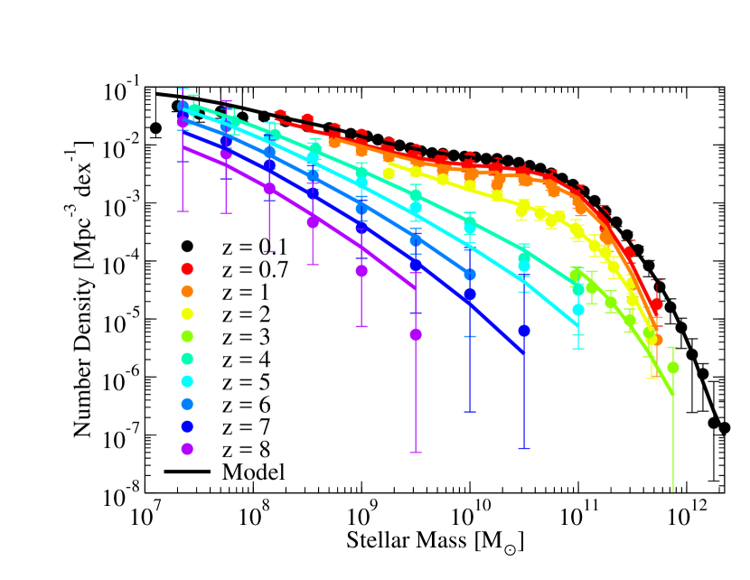
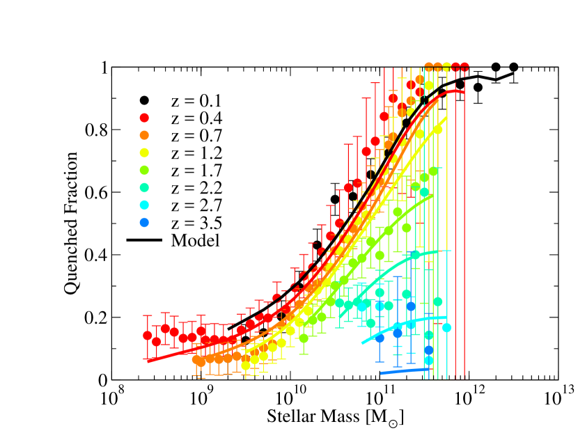
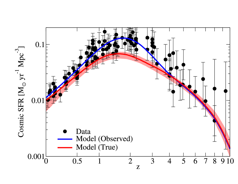
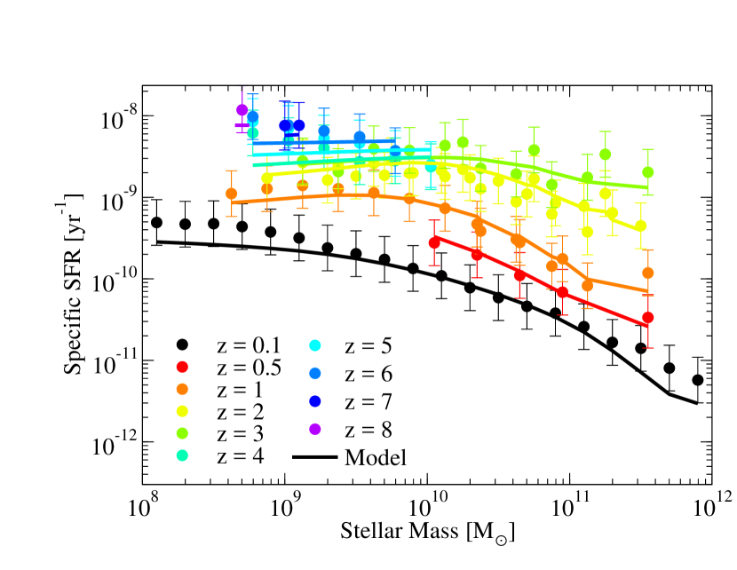
Figure 2: Left panel: Comparison between observed stellar mass functions (Appendix C.2) and the best-fitting model. References for observations are in Table 5. Right panel: Comparison between observed quenched fractions (Appendix C.6) and the best-fitting model. Observed quenched fractions are adapted from Bauer et al. (2013), Moustakas et al. (2013), and Muzzin et al. (2013). Notes: almost all data from both panels were used to constrain the best-fitting model. The exceptions are the $z=4-8$ SMFs from Song et al. (2016), which are shown for comparison only; these were not used in the fitting as the same underlying data is already represented in the $z=4-8$ UVLFs and the UV–SM relations (Fig. 4). The Bolshoi-Planck simulation used is incomplete for low-mass haloes, contributing to an underestimation of the SMF below $10^{7}\;\mathrm{M}_{\odot}$ at $z=0$, a limit which rises smoothly to $10^{8}\;\mathrm{M}_{\odot}$ by $z\sim 8$.

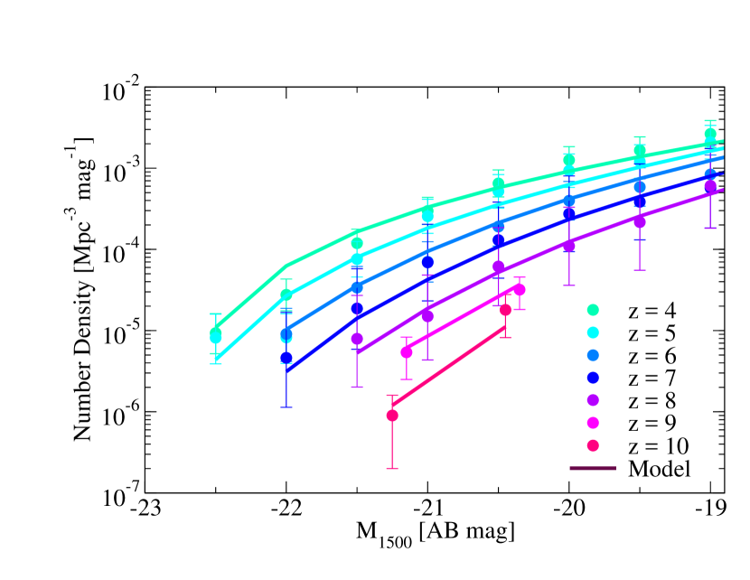
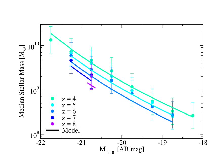
Figure 3: Left panel: Comparison between observed cosmic star formation rates (CSFRs; Appendix C.3) and the best-fitting model; references are in Table 6. The red line shows the inferred true cosmic star formation rate, and the red shaded region shows the $16^{\mathrm{th}}-84^{\mathrm{th}}$ percentile range from the posterior distribution. The blue line shows the best-fitting model after accounting for redshift-dependent observational systematic offsets. Right panel: Comparison between observed specific star formation rates (Appendix C.3) and the best-fitting model; references are in Table 7. Notes: all data from both panels were used to constrain the best-fitting model. For CSFRs at $z>4$, data from both magnitude-limited ($M_{\mathrm{1500}}<-17$) and total CSFRs (from long GRBs) are shown. In Bolshoi-Planck, resolution limits mean that the total CSFR for all modeled galaxies is nearly identical to the CSFR for galaxies with $M_{\mathrm{1500}}<-17$. See Appendix C.3 for further discussion.

Figure 4: Left panel: Comparison between observed UV luminosity functions (Appendix C.5) from Finkelstein et al. (2015a) and Bouwens et al. (2016a) and the best-fitting model. Right panel: comparison between median UV–stellar mass relationships (Appendix D) for the best-fitting model and the observed results rederived in this paper from SED stacks in Song et al. (2016). Notes: all data from both panels were used to constrain the best-fitting model. The Bolshoi-Planck simulation used is incomplete for low-mass haloes, so we do not fit to UV luminosity functions for $M_{1500}>-19$.

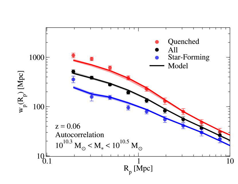
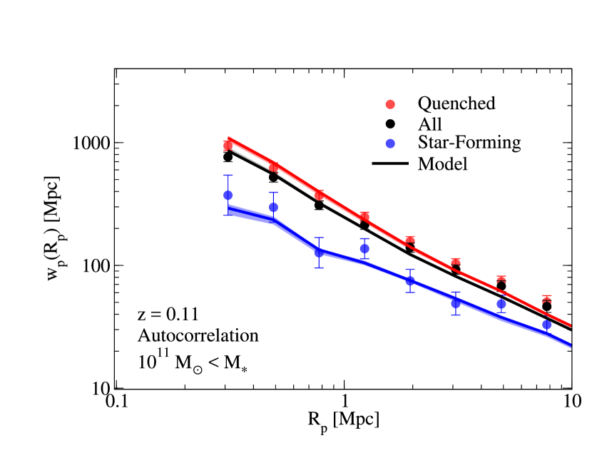
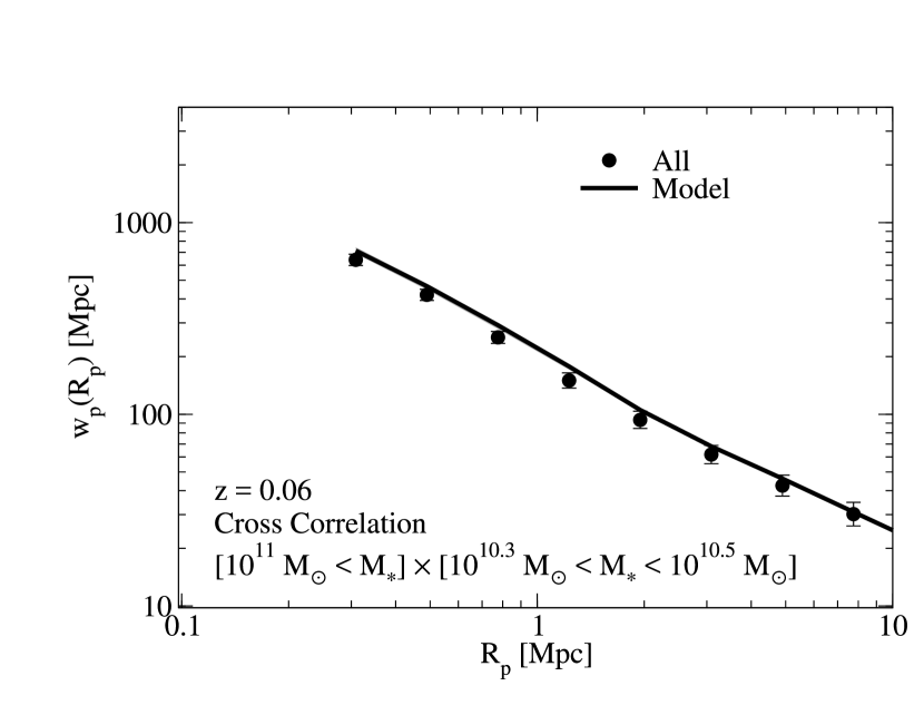
Figure 5: Comparison between galaxy autocorrelation and cross correlation functions at $z\sim 0$ for the best-fitting model and the observed results rederived from the SDSS in Appendix C.7. Notes: all data from all panels were used to constrain the best-fitting model. Observational errors shown are jackknife estimates from the observational sample. Actual fitting used covariance matrices as detailed in Appendix C.7.

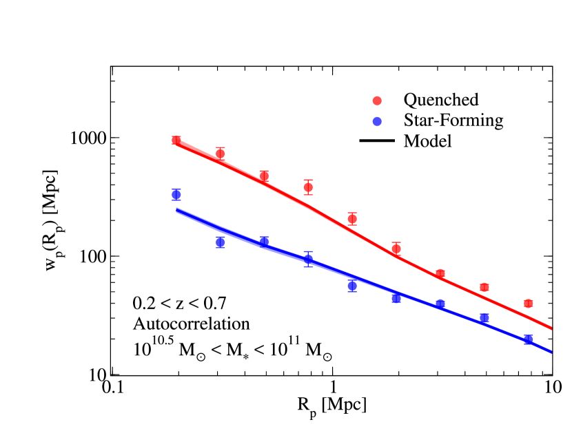
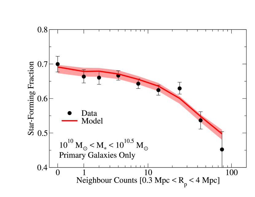
Figure 6: Comparison between observed galaxy autocorrelation functions at $z\sim 0.5$ (Coil et al., 2017, i.e., PRIMUS) and the best-fitting model. Notes: all data from this panel were used to constrain the best-fitting model. Redshift errors for PRIMUS were rederived according to Appendix C.7.

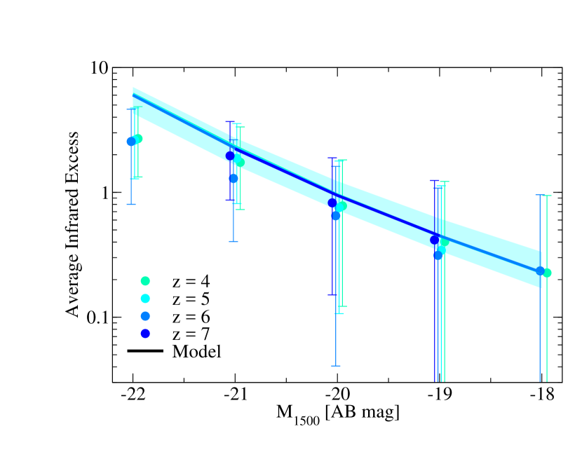
Figure 7: Comparison between primary galaxy quenched fractions as a function of neighbour density in the SDSS (derived in Appendix C.8) and the best-fitting model (red line; $16^{\mathrm{th}}-84^{\mathrm{th}}$ percentile range shown as red shaded region). As discussed in §2.2, this provides an approximate probe of the correlation between central halo and galaxy assembly. Primary galaxies are defined as being the largest galaxy within a projected distance of 500 kpc and a redshift distance of 1000 km s^-1. Neighbours are defined as galaxies with masses within a factor $0.3-1$ of the primary galaxy. Notes: all data from this panel were used to constrain the best-fitting model.

Figure 8: Average infrared excess (IRX) as a function of observed UV luminosity from ALMA data at $z=4-7$ (Bouwens et al., 2016b) and the best-fitting model (lines; $16^{\mathrm{th}}-84^{\mathrm{th}}$ percentile range at $z=4$ shown as cyan shaded region). Notes: all data from this panel were used to constrain the best-fitting model. Observational data are offset slightly in UV luminosity to increase clarity between different redshifts. The best-fitting model evolves very little with redshift, so model lines are not distinguishable.

3.5 Observational Systematics

Systematic uncertainties in stellar masses and SFRs arise from modeling assumptions for stellar population synthesis (SPS), dust, metallicity, and star formation history (Conroy et al., 2009; Conroy, 2013; Behroozi et al., 2010, 2013e). The dominant effect is a redshift-dependent offset between true and observed values for both stellar masses and SFRs, parametrized here as

$$\mu\equiv SM_{\mathrm{obs}}-SM_{\mathrm{true}}=\mu_{0}+\mu_{a}(1-a).$$ (25)

This is constrained by tension between CSFRs and evolution in SMFs (e.g., Wilkins et al., 2008; Yu & Wang, 2016), as well as tension between SSFRs and observed UVLFs. Following Behroozi et al. (2013e), we set the prior width on $\mu_{0}$ and $\mu_{a}$ to 0.14 and 0.24 dex, respectively.

We also include a redshift-dependent offset that affects only SFRs, motivated by strong tensions between observed radio and UV+IR SSFRs and evolution in SMFs that peaks at $z=2$ (Leja et al., 2015, see also Appendix C.4). This coincides with existing tensions between SSFRs from observations and SSFRs from modern hydrodynamical simulations (e.g., Sparre et al., 2015; Davé et al., 2016), as well as tensions between IR and SED-fit SFR indicators (Fang et al., 2018):

$$SFR_{\mathrm{obs}}-SFR_{\mathrm{true}}=\mu+\kappa\exp\left(-\frac{(z-2)^{2}}{2}\right).$$ (26)

The prior width on $\kappa$ is set to 0.24 dex (Table 3), matching the prior on $\mu_{a}$.

Offsets could also be mass-dependent (see Li & White 2009 and Appendix C) and SSFR-dependent (Behroozi et al., 2013e). Tension between SSFRs and SMFs could also constrain a mass-dependent offset; however, the fact that errors on the SMF are much tighter than errors on the SSFR would result in our MCMC algorithm recruiting the parameter so as to better fit the shape of the SMF (i.e., overfitting). SSFR-dependent offsets could be constrained by the amplitude of the autocorrelation function—however, this is extremely degenerate with sample variance. Hence, we use the simple Eqs. 25 and 26 in this work to parametrize systematic offsets.

Random errors in recovering stellar masses can also cause Eddington bias in the massive-end shape of the SMF (Behroozi et al., 2010, 2013e; Grazian et al., 2015). Since the errors grow with redshift, they impact the inferred mass growth of massive galaxies. Here, we use the same redshift dependence as Behroozi et al. (2013e), but limit the maximum scatter at high redshift:

$$\sigma_{\mathrm{SM,obs}}=\min(\sigma_{SM,0}+\sigma_{SM,z}z,0.3)\,\mathrm{dex}.$$ (27)

For example, Grazian et al. (2015) find a scatter of $\sim 0.2$ dex at $z=6$ in the distribution of SMs for $\sim 10^{11}\;\mathrm{M}_{\odot}$ galaxies; this expands to 0.3 dex after accounting for additional scatter from photometric redshifts, photometry, code choices (including finite age/metallicity grids), and other sources (see Mobasher et al. 2015 for a review).

Similarly, random log-normal errors in observed SFRs can broaden the observed SFR distribution and lead to enhanced average CSFRs, as the average (in linear space) of a log-normal distribution is higher than the median. We adopt

$$\sigma_{\mathrm{SFR,obs}}=\sqrt{0.3^{2}-\sigma_{\mathrm{SF}}^{2}}\mathrm{dex},$$ (28)

so that the combined intrinsic plus observed main-sequence scatter is $0.3$ dex, consistent with Speagle et al. (2014).

All observables are subject to volume-weighting effects; some are also subject to binning effects. When modeling observables, we use identical binning, and we also use volume-weighting across the reported redshift range. For a given observable $X$ reported for $z_{1}<z<z_{2}$, we thus simulate the observation as

$$X_{\mathrm{model}}=\frac{\int_{z_{1}}^{z_{2}}X(z)dV(z)}{V(z_{2})-V(z_{1})},$$ (29)

where $V(z)$ is the enclosed volume out to redshift $z$. For correlation functions and higher-order statistics that depend on spectroscopic redshifts, we include redshift-space distortions from halo peculiar velocities. We also include 30 km s^-1 of combined galaxy–halo velocity bias and redshift-fitting errors, assumed to be normally distributed (Guo et al., 2015). For the grism-based redshifts in PRIMUS, we model the redshift errors as $\sigma_{z}/(1+z)=0.0033$, as discussed in Appendix C.7.

The initial mass function (IMF) is known to vary with galaxy velocity dispersion (Conroy & van Dokkum, 2012; Conroy et al., 2013; Geha et al., 2013; Martín-Navarro et al., 2015; La Barbera et al., 2016; van Dokkum et al., 2017). However, broadband photometric luminosities depend largely on the mass in $>1\;\mathrm{M}_{\odot}$ stars, resulting in a constant overall mass offset for different IMF assumptions. As a result, the main body of this paper adopts the same assumption as for all the observational results with which we compare—namely, a universal Chabrier (2003) IMF. Appendix G shows how derived stellar mass—halo mass relationships would change for a halo mass-dependent IMF.

4 Results

We discuss best-fitting parameters and the comparison to observables in §4.1, the stellar mass–halo mass relation in §4.2, average SFRs and quenched fractions in dark matter haloes in §4.3, average star formation histories in §4.4, individual stochasticity in SFRs in §4.5, correlations between galaxy and halo assembly in §4.6, satellite quenching in §4.7, in-situ vs. ex-situ star formation in §4.8, predictions for future observations in §4.9, systematic uncertainties in §4.10, and additional online data in §4.11.

4.1 Best-fitting Parameters and Comparison to Observables

We explored model posterior space with 100 simultaneous MCMC walkers, totaling $\sim$500k MCMC steps and $400$k CPU hours. Convergence was approached by running the chains for $10$ autocorrelation times. The best-fitting model was found by starting from the average of all walker positions during the final 400 steps and then using a gradient descent algorithm to converge on the model with lowest $\chi^{2}$.

The best-fitting model is able to match all data in §2.2, including stellar mass functions (SMFs; Fig. 4, left panel), quenched fractions (QFs; Fig. 4, right panel), cosmic star formation rates (CSFRs; Fig. 4, left panel), specific star formation rates (SSFRs; Fig. 4, right panel), high-redshift UV luminosity functions (UVLFs; Fig. 4, left panel), high-redshift UV–stellar mass relations (UVSMs; Fig. 4, right panel), correlation functions (CFs; Figs. 5 and 8), the dependence of the quenched fraction of central galaxies as a function of environment (Fig. 8), and the average infrared excess as a function of UV luminosity (Fig. 8). Calculating the true number of degrees of freedom for the observational data is difficult; for example, covariance matrices are unavailable for most SMFs, QFs, UVLFs, etc. in the literature. Yet, for 1069 observed data points and 44 parameters, the naive reduced $\chi^{2}$ of the best-fitting model is 0.36, suggesting a reasonable fit.

The best-fitting model and 68% confidence intervals for parameters are presented in Appendix H, and parameter correlations are discussed in Appendix I. Key physical aspects of the parameterization include the star formation rate for star-forming galaxies and the quenched fraction as a function of $v_{\mathrm{Mpeak}}$ (shown in Fig. 15), as well as the correlation between galaxy and halo growth (shown in Fig. 20). Posterior distributions of many other quantities (e.g., the stellar mass–halo mass relation, cross-correlation functions, satellite and quenching statistics, etc.) are described in the following sections and are available online.

4.2 The Stellar Mass – Halo Mass Relation for z=0 to z=10

4.2.1 Stellar Mass – Halo Mass Ratios

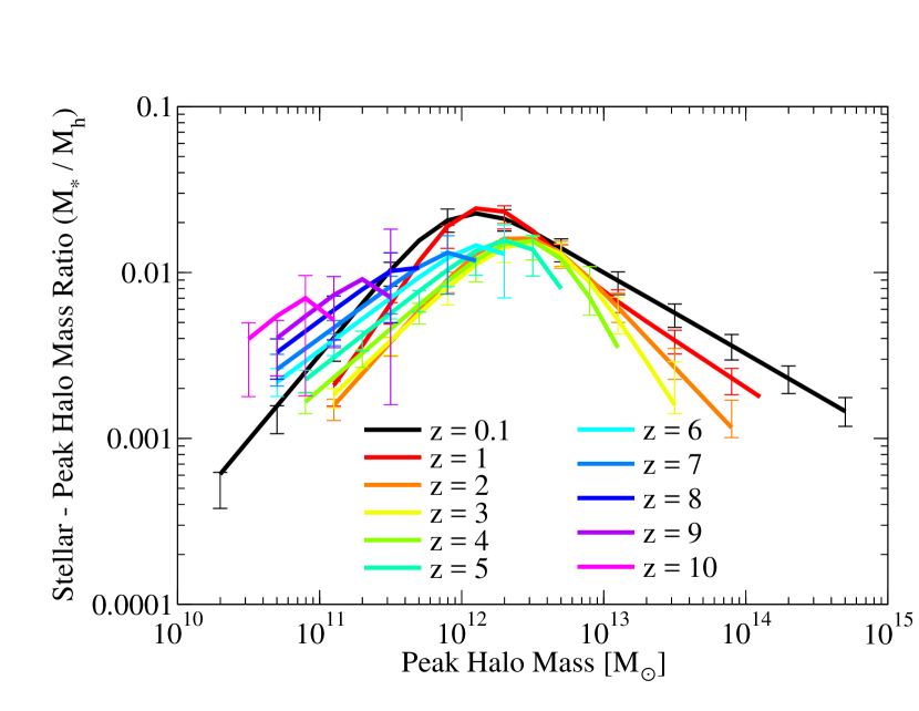
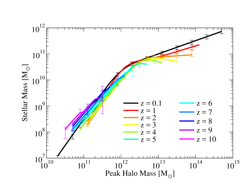
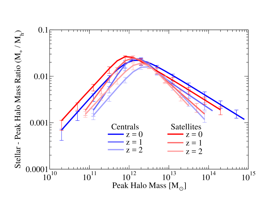
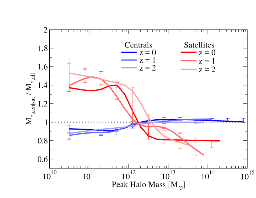
Figure 9: Left panel: best-fitting median ratio of stellar mass to peak halo mass ($M_{\mathrm{peak}}$) as a function of $M_{\mathrm{peak}}$ and $z$. Right panel: best-fitting median stellar mass as a function of $M_{\mathrm{peak}}$ and $z$. Error bars in both panels show the 68% confidence interval for the model posterior distribution. Notes: see Figs. 35-36 for a comparison with past results. See Appendix J for fitting formulae.

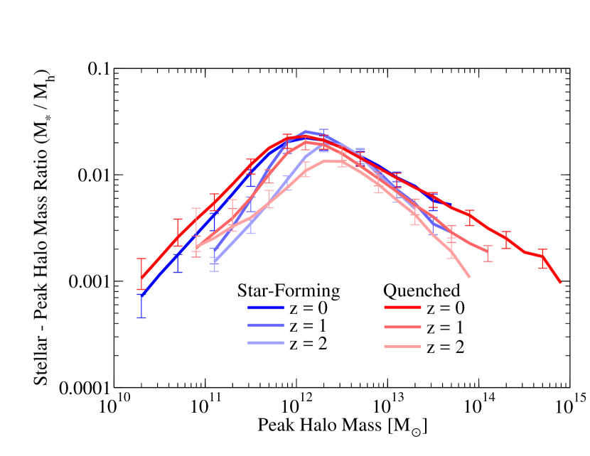
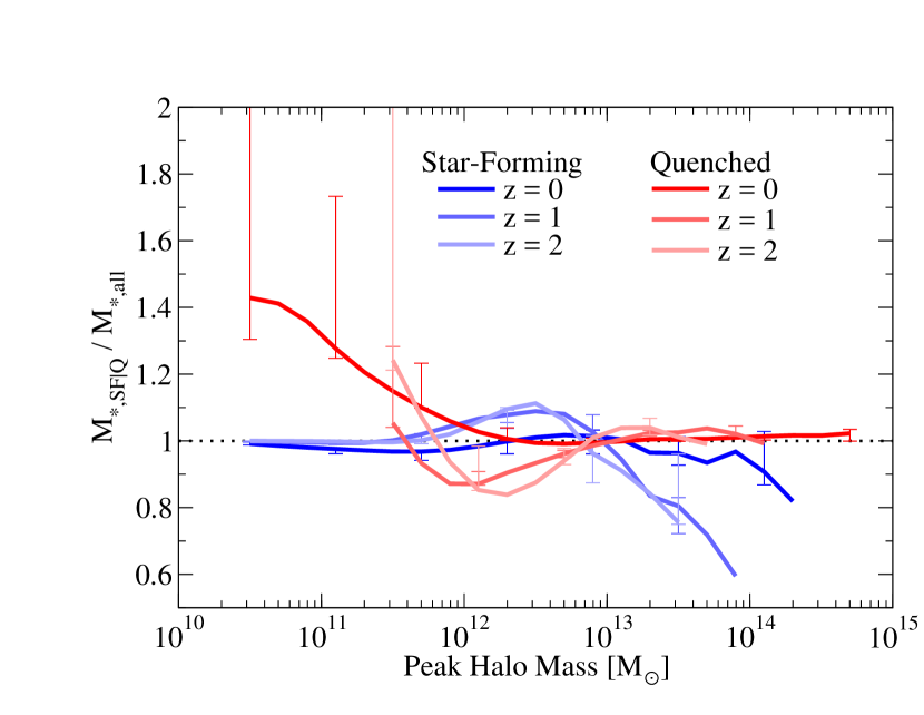
Figure 10: The best-fitting median ratio of stellar mass to peak halo mass ($M_{\mathrm{peak}}$) for central and satellite galaxies (left panel) compared to the ratio for all galaxies (right panel). Error bars in both panels show the 68% confidence interval for the model posterior distribution. See Appendix J for fitting formulae.

Figure 11: The best-fitting median ratio of stellar mass to peak halo mass ($M_{\mathrm{peak}}$) for star-forming and quenched galaxies (left panel) compared to the ratio for all galaxies (left panel). Error bars in both panels show the 68% confidence interval for the model posterior distribution. Notes: quiescent galaxies in low-mass ($<10^{12}\;\mathrm{M}_{\odot}$) haloes are very rare at $z\geq 1$, contributing to substantial uncertainties in their stellar mass–halo mass relations. Due to scatter in stellar mass at fixed halo mass, a higher stellar mass for star-forming galaxies at fixed halo mass does not necessarily imply a lower halo mass for star-forming galaxies at fixed galaxy mass; see §39 for discussion. See Appendix J for fitting formulae.

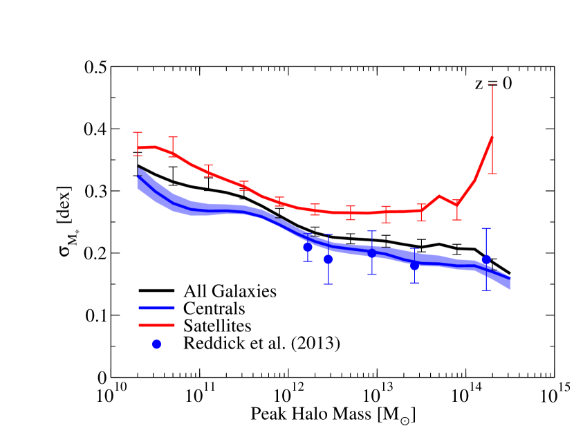
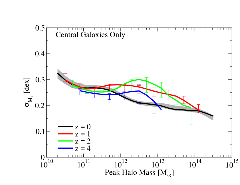
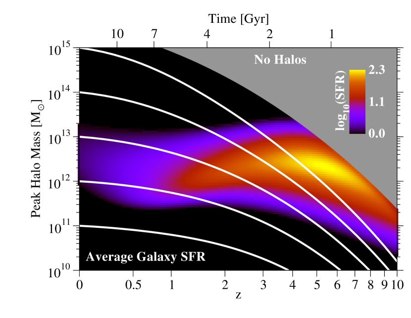
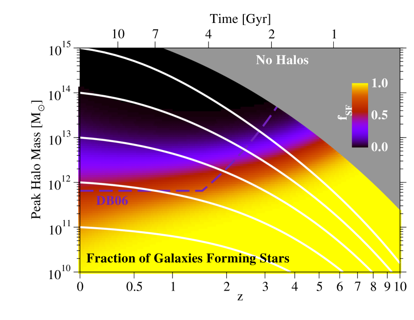
Figure 12: Left panel: best-fitting scatter in stellar mass at fixed $M_{\mathrm{peak}}$, split for central and satellite galaxies at $z=0$, compared with the results for central galaxies in Reddick et al. (2013). Right panel: best-fitting scatter in stellar mass at fixed peak halo mass ($M_{\mathrm{peak}}$) for central galaxies as a function of $M_{\mathrm{peak}}$ and $z$. Error bars and shaded regions in both panels show the 68% confidence interval for the model posterior distribution.

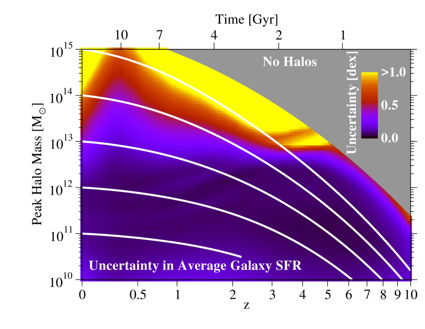
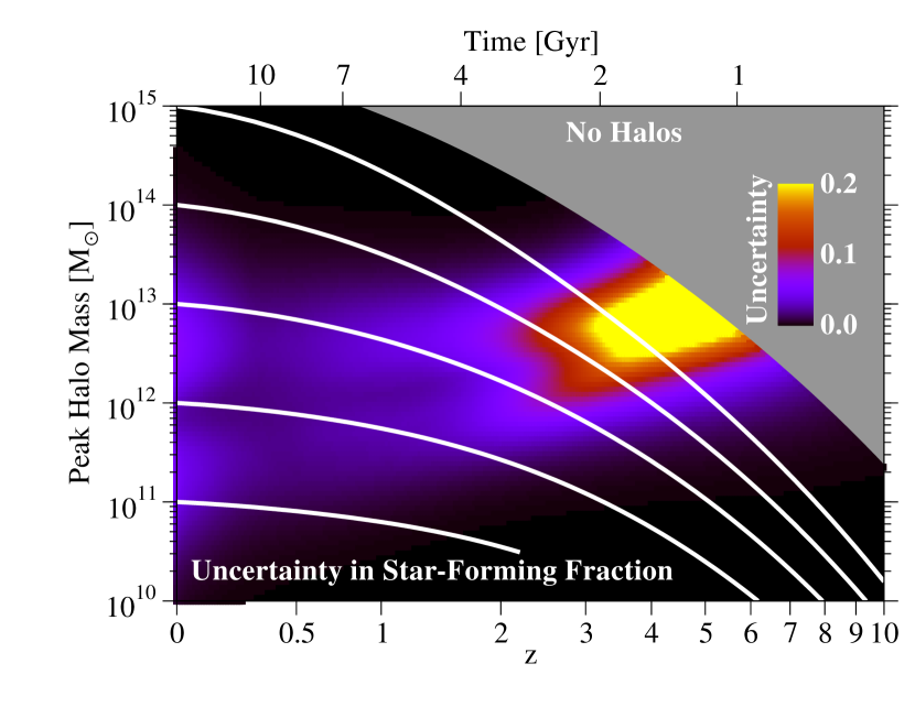
Figure 13: Left panel: Average star formation rates in galaxies as a function of halo mass and redshift. Right panel: Average star-forming fractions as a function of halo mass and redshift. The purple line marks the predicted transition in Dekel & Birnboim (2006) between cold flows reaching the central galaxy (below the line) and not reaching it due to shock heating (above the line). In both panels, white lines mark median halo growth trajectories, and the gray region marks where no haloes are expected to exist in the observable Universe. A robust upturn in the star-forming fraction to higher redshifts is visible (§4.3).

Figure 14: Left panel: formal model uncertainty (half of the $16^{\mathrm{th}}-84^{\mathrm{th}}$ percentile range) in average galaxy SFRs (Fig. 14, left panel). Right panel: formal model uncertainty (half of the $16^{\mathrm{th}}-84^{\mathrm{th}}$ percentile range) in average galaxy star-forming fractions (Fig. 14, right panel).

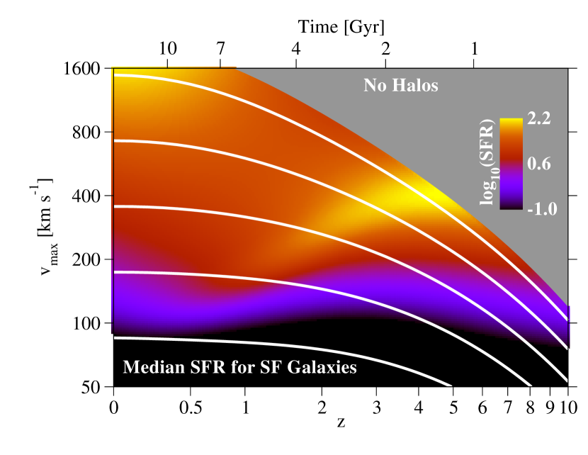
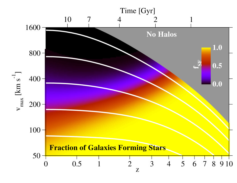
Figure 15: Left panel: Median star formation rate for star-forming haloes as a function of $v_{\mathrm{Mpeak}}$ and $z$ ($SFR_{\mathrm{SF}}$; Eqs. 4$-$11). Right panel: star-forming fraction ($1-f_{\mathrm{Q}}$) as a function of $v_{\mathrm{Mpeak}}$ and $z$ (Eqs. 12$-$15).

We show the median stellar mass — peak halo mass ratio (SMHM ratio) for all galaxies in Fig. 11, which agrees with past measurements (§39). Although the SMHM ratio has little net change from $z=0$ to $z\sim 5$, this study supports significant evolution at $z>5$ (see also §5.10). Fitting formulae for median SMHM ratios are presented in Appendix J.

As shown in Fig. 11, we find that central and satellite haloes have significantly different SMHM ratios. At low halo masses, satellite quenching timescales are long (§4.7), so they grow in stellar mass while $M_{\mathrm{peak}}$ remains fixed, leading to higher SMHM ratios. At high halo masses, the dominant growth channel is via mergers (§4.8), which are reduced for satellites due to high relative velocities; hence, they have lower SMHM ratios than centrals.

We also find that star-forming and quenched galaxies have significantly different SMHM ratios (Fig. 11) except at $z\sim 0$. At low masses ($M_{\mathrm{peak}}\ll 10^{12}\;\mathrm{M}_{\odot}$) and redshifts $z>0$, most quenched galaxies stopped forming stars only recently, leading to relatively small differences. At high masses ($M_{\mathrm{peak}}\gg 10^{12}\;\mathrm{M}_{\odot}$), the only star-forming galaxies are those whose haloes have formed very recently, resulting in less time for satellites to merge and contribute stellar mass.

For intermediate masses ($M_{\mathrm{peak}}\sim 10^{12}\;\mathrm{M}_{\odot}$), the picture is more complex. These haloes quench and rejuvenate (§4.5) while mass accretion continues. Hence, galaxies that are star-forming tend to have higher SMHM ratios (galaxies growing faster relative to their haloes), whereas those that are quenched have lower SMHM ratios (no galaxy growth but continued halo growth). These differences are more evident at $z=2$, where the ratio of galaxy SSFRs to halo specific accretion rates is higher (e.g., Behroozi & Silk, 2015). At $z=0$, galaxy growth is less rapid, and so galaxies have less time to grow significantly between periods of quenching and rejuvenation driven by halo mass accretion. The difference between SMHM ratios for quiescent and star-forming galaxies is thus sensitive to the amount of quenching and rejuvenation, but in practice, the observed difference is just as sensitive to systematic errors in the stellar masses used (Appendix C.2).

4.2.2 Scatter in the Stellar Mass – Halo Mass Relation

We also show constraints on scatter in the SMHM relation in Fig. 14. Our primary observational constraint on scatter comes from correlation functions (Figs. 5 and 8), but this is somewhat degenerate with the orphan fraction (see Appendix B). Without orphans, our model cannot match autocorrelation functions for low-mass galaxies, which are largely unaffected by scatter. As a result, autocorrelation functions for larger galaxies (which are more sensitive to scatter) can be reproduced with somewhat larger scatters than previous works that did not include orphans (e.g., Reddick et al., 2013). It is possible that a more complicated orphan model could reduce the need for additional scatter; constraining such a model would require additional observational data beyond what is used here (see §5.8).

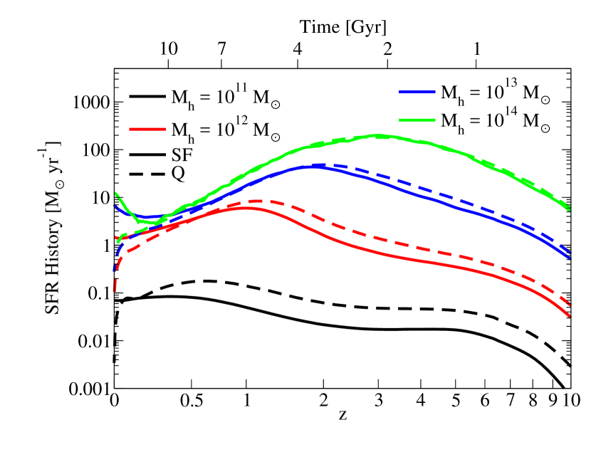
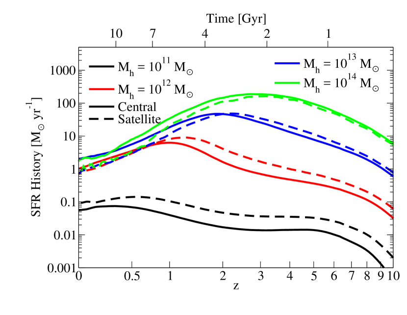
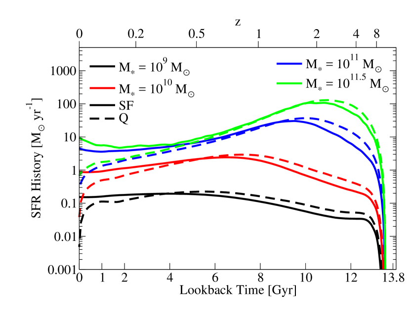
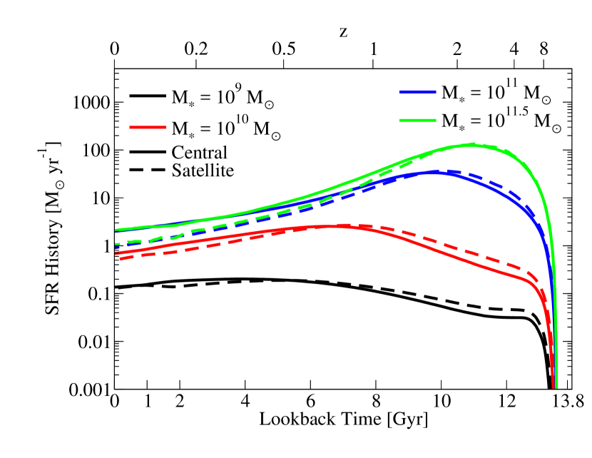
Figure 16: Left panel: average star formation histories for star-forming and quiescent galaxies, as a function of peak $z=0$ halo mass ($M_{\mathrm{peak}}$) for our best-fitting model. Right panel: same, except split for central and satellite galaxies. Notably, satellites are binned according to the peak historical mass of the satellite halo, as opposed to their host halo. For both panels, bin widths are $\pm 0.25$ dex; e.g., the label $M_{h}=10^{11}\;\mathrm{M}_{\odot}$ corresponds to $10.75<\log_{10}(M_{\mathrm{peak}}/\;\mathrm{M}_{\odot})<11.25$.

Figure 17: Left panel: average star formation histories for star-forming and quiescent galaxies, as a function of $M_{\ast}$ at $z=0$ for our best-fitting model. These are shown as a function of lookback time to emphasize the recent differences that have greater observable effects. Right panel: same, except split for central and satellite galaxies. For both panels, bin widths are $\pm 0.25$ dex; e.g., the label $M_{\ast}=10^{11}\;\mathrm{M}_{\odot}$ corresponds to $10.75<\log_{10}(M_{\ast}/\;\mathrm{M}_{\odot})<11.25$.

In the model, satellites have much larger scatter than central galaxies (Fig. 14, left panel), due to the orbit-dependence of continued star formation after infall. Similarly, quenched galaxies have larger scatter than star-forming galaxies, as quenched populations have larger satellite fractions. We also find lower scatter in stellar mass towards higher halo masses. This results from an increasing fraction of mass growth via mergers (Fig. 27; see also Moster et al., 2013; Behroozi et al., 2013e; Gu et al., 2016); other empirical models (e.g., Moster et al., 2018) show similar trends.

Our current constraints are consistent with either no redshift evolution in the scatter or a slight increase toward higher redshifts (Fig. 14, right panel). Increased scatter is most prominent for haloes near $10^{12}\;\mathrm{M}_{\odot}$. Haloes near this mass grow primarily by star formation, and so are dramatically affected by quenching (see also Fig. 23, right panel) if it is not perfectly correlated with mass growth. Galaxies in lower-mass haloes are mostly star-forming and hence have smaller variations in star formation histories (see also Fig. 23, left panel). Galaxies in larger haloes grow primarily by merging, which is more correlated with halo mass growth. Indeed, had our model correlated quenching directly with halo mass growth instead of change in $v_{\mathrm{max}}$, the overall scatter would be lower and the feature near $10^{12}\;\mathrm{M}_{\odot}$ would not exist (see Moster et al., 2018).

4.3 Average SFRs and Star-Forming Fractions

Average SFRs and star-forming fractions for the best-fitting model are shown as a function of $M_{\mathrm{peak}}$ and $z$ for all galaxies in Fig. 14. Similar to past results (e.g., Behroozi et al., 2013e), high mass haloes exhibit a short period of very intense star formation and then quench, whereas lower-mass haloes have much more extended star formation histories. The most notable difference from previous modeling is an improved treatment of quenching in massive haloes (§3.2), which reduces their expected star formation rates. We caution that star formation rates for central galaxies in massive haloes are nonetheless very hard to measure observationally, so the values in Fig. 14 for massive quenched haloes should be treated as upper limits (see also the formal uncertainties in Fig. 14, left panel).

At $z>1$, Fig. 14 shows a strong correlation between halo mass and quenching; a difference of $\lesssim$1.5 dex in host halo mass separates populations that are nearly $100\%$ star-forming from those that are nearly 100% quenched. For $z<1$, satellite quenching becomes more important, and so quenched galaxies appear over a broader range in halo mass. As discussed in later sections, haloes with moderate quenched fractions (30-70%) are more susceptible to quenching via differences in assembly rates.

At fixed halo mass, average quenched fractions for galaxies decrease significantly with increasing redshift. The SMHM relation evolves relatively little from $z=0-4$ (Fig. 11), whereas $f_{\mathrm{Q}}(M_{\ast})$ evolves significantly (Fig. 4), requiring $f_{\mathrm{Q}}(M_{h})$ to evolve significantly with redshift as well. This is qualitatively (but not quantitatively) in agreement with Dekel & Birnboim (2006), as discussed in §5.2. Formal uncertainties are shown in Fig. 14 (right panel), and are under 10% for almost all redshifts and halo masses.

We show the underlying constraints on $SFR_{\mathrm{SF}}(v_{\mathrm{Mpeak}},z)$ and $f_{\mathrm{Q}}(v_{\mathrm{Mpeak}},z)$ in Fig. 15. The average SFR in Fig. 14 is the product of the left and right panels of Fig. 15, with a small correction for scatter. The left panel suggests that when galaxies in massive haloes are able to form stars, they do so extremely rapidly—qualitatively consistent with observations of the Phoenix cluster (McDonald et al., 2013) and precipitation theory (Voit et al., 2015). However, the highest star-formers on average are in lower-mass haloes at higher redshifts, where the quenched fractions are much lower.

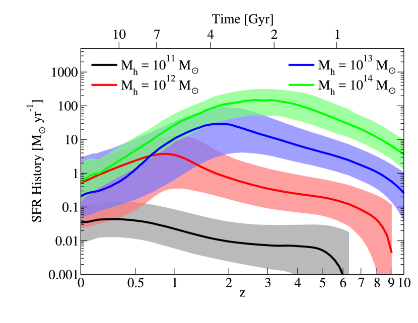
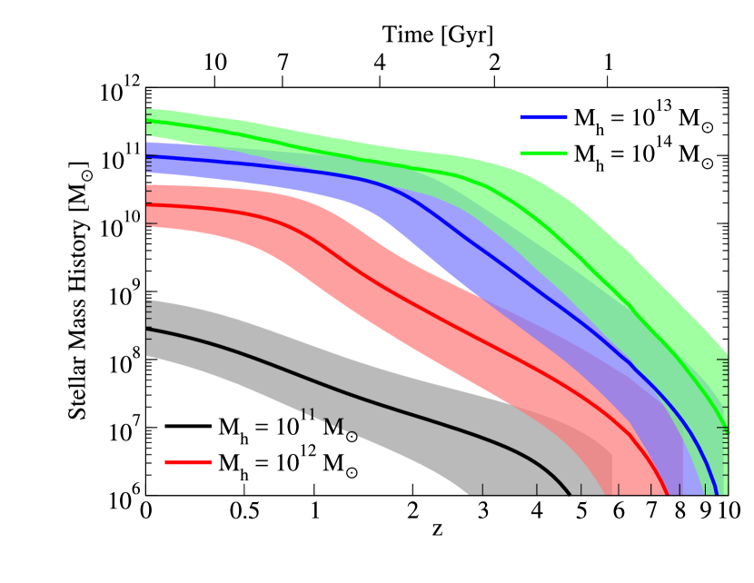
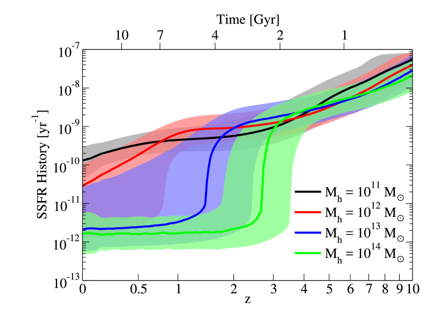
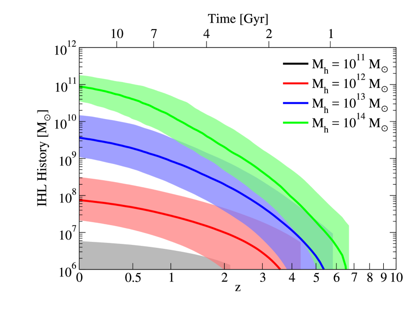
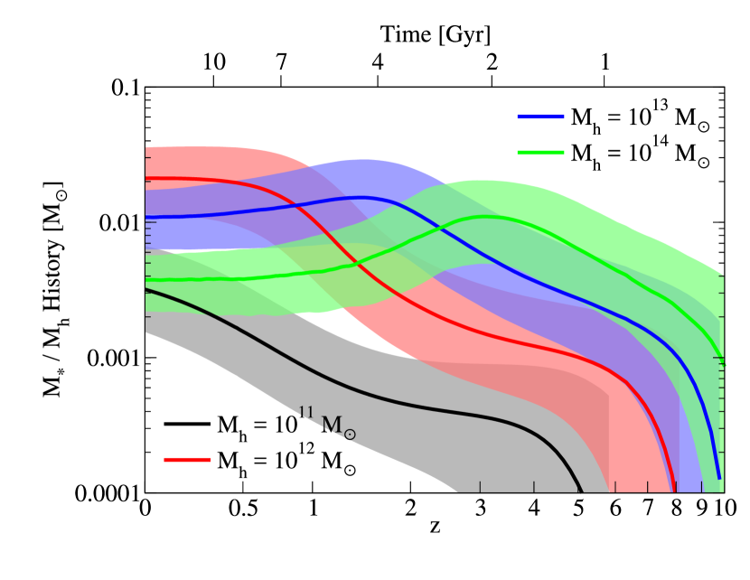
Figure 18: Top left: total (including mergers) star formation histories for haloes in bins of $M_{\mathrm{peak}}$ for our best-fitting model; coloured regions indicate the $16^{\mathrm{th}}-84^{\mathrm{th}}$ percentile range among different haloes in the best-fitting model. Top right: same, with main progenitor stellar mass histories. Middle left: same, with main progenitor SSFR histories. Middle right: same, with main progenitor intrahalo light (IHL) histories. Bottom left: same, with main progenitor $M_{\ast}/M_{\mathrm{peak}}$ ratio histories. Bottom right: same, with main progenitor IHL / $M_{\ast}$ ratio histories. For all panels, bin widths are $\pm 0.25$ dex; e.g., the label $M_{h}=10^{11}\;\mathrm{M}_{\odot}$ corresponds to $10.75<\log_{10}(M_{\mathrm{peak}}/\;\mathrm{M}_{\odot})<11.25$. Notes: Quiescent SSFRs in our models are fixed to $10^{-11.8}$ yr^-1 (§3.2), explaining why massive haloes’ SSFRs are close to this value at low redshifts.

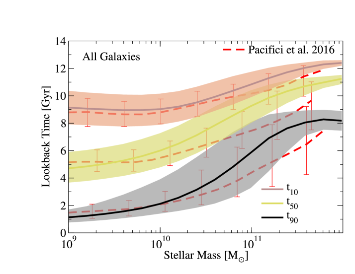
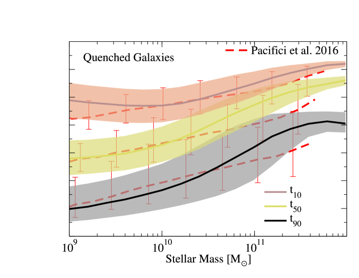
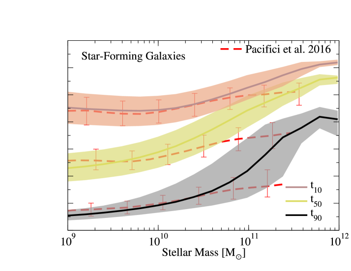
Figure 19: Lookback times for stellar mass assembly thresholds. Left panel: median lookback times for our best-fitting model at which progenitors of $z=0$ galaxies reached $10\%$ (brown line), 50% (sandy line) and 90% (black line) of their $z=0$ stellar mass. Shaded regions show the 16${}^{\mathrm{th}}-84^{\mathrm{th}}$ percentile ranges of lookback times across different $z=0$ galaxies. Red dashed lines show the comparison with Pacifici et al. (2016); error bars show the equivalent $16^{\mathrm{th}}-84^{\mathrm{th}}$ percentile range. Middle panel: same, for quenched galaxies. Right panel: same, for star-forming galaxies.

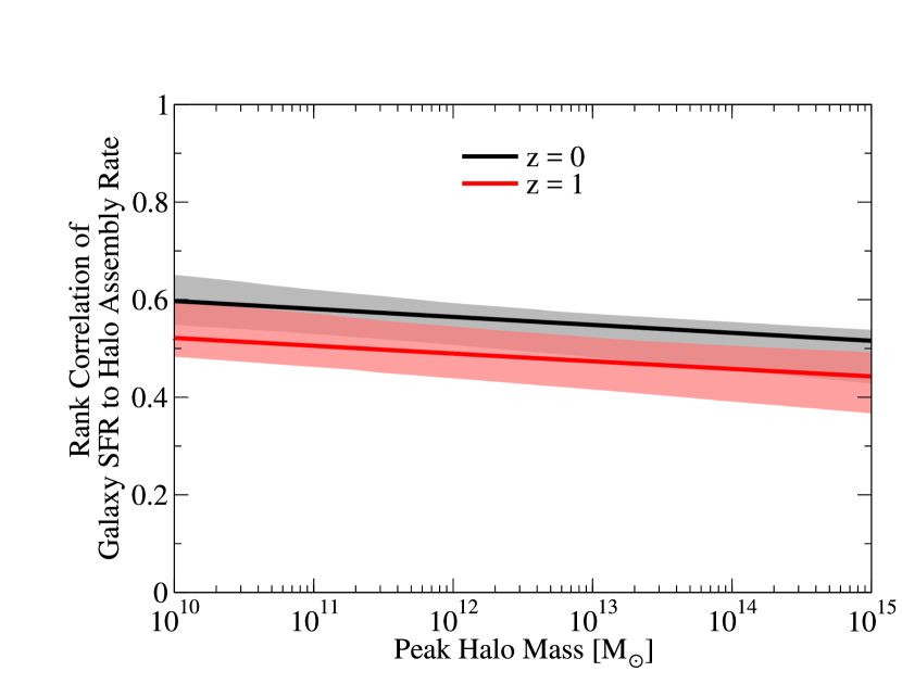
Figure 20: Constraints on the rank correlation coefficient ($r_{c}$; Eq. 16) between halo growth ($\Delta v_{\mathrm{max}}$; Eq. 1) and galaxy SFR, as a function of host halo mass at $z=0$. Shaded regions show the $16^{\mathrm{th}}-84^{\mathrm{th}}$ percentile range across the model posterior space.

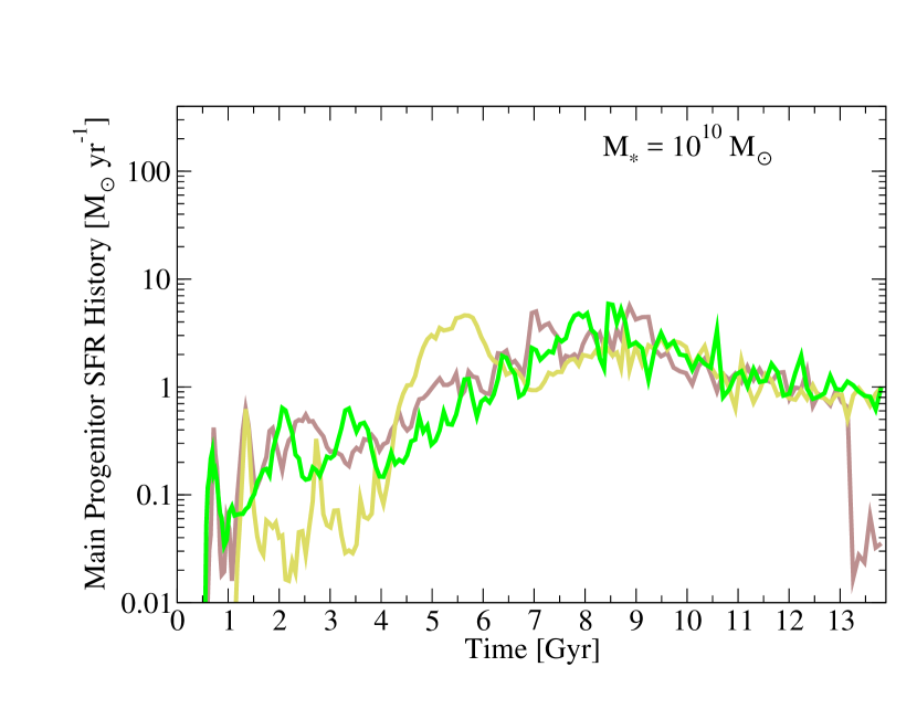
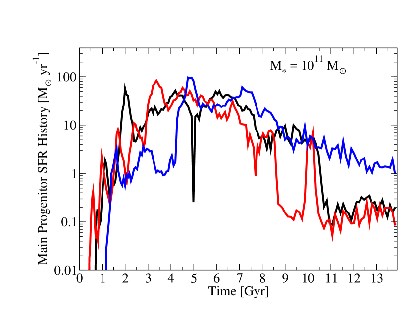
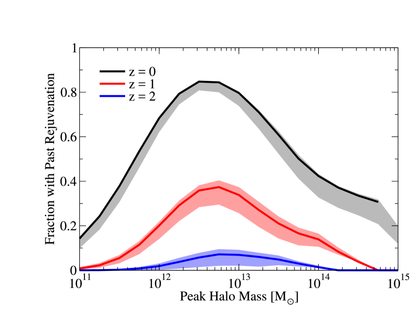
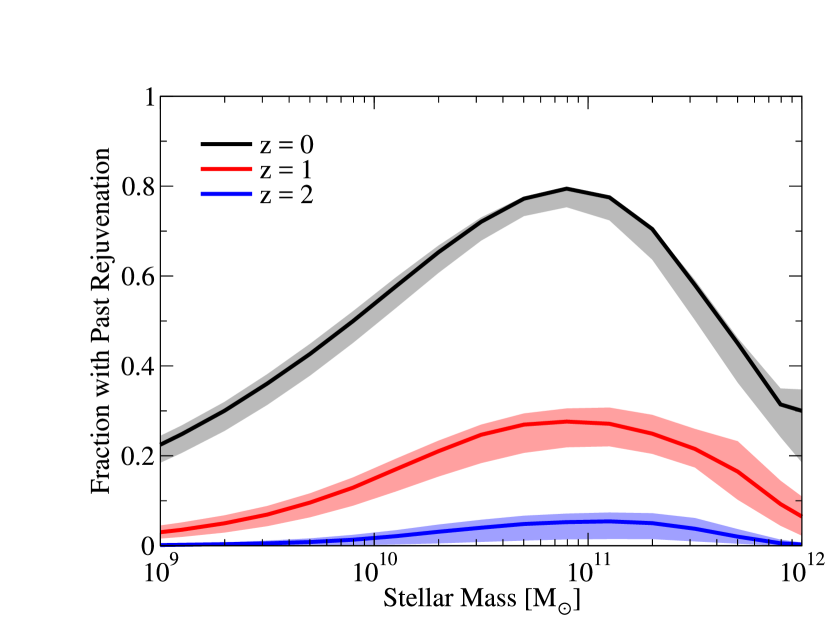
Figure 21: Left panel: main progenitor star formation histories for several $M_{\ast}=10^{10}\;\mathrm{M}_{\odot}$ galaxies at $z=0$ from the best-fitting model. Right panel: progenitor star formation histories for several $M_{\ast}=10^{11}\;\mathrm{M}_{\odot}$ galaxies at $z=0$ from the best-fitting model. These show significantly more variation than their lower-mass counterparts, due to periods of quenching and rejuvenation.

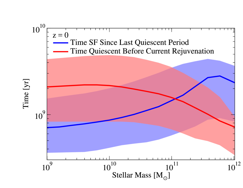
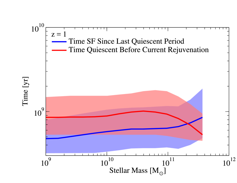
Figure 22: Left panel: fraction of $z=0$ haloes whose galaxies quenched and then rejuvenated in the past; rejuvenation is defined as at least $300$ Myr of quiescence, followed by at least 300 Myr of star formation. Right panel: same, as a function of $z=0$ galaxy mass. In both panels, shaded regions show the $16^{\mathrm{th}}-84^{\mathrm{th}}$ percentile range across the model posterior space.

Figure 23: Left panel: For rejuvenated galaxies at $z=0$ (see text), the median times spent in the rejuvenated star-forming phase (blue line) and in the quiescent phase prior to rejuvenation (red line). Shaded regions show the $16^{\mathrm{th}}-84^{\mathrm{th}}$ percentile range for individual galaxies in the best-fitting model. Right panel: same, at $z=1$.

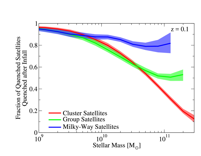
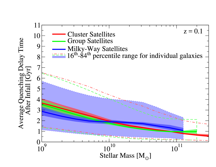
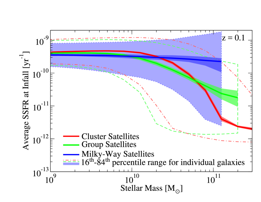
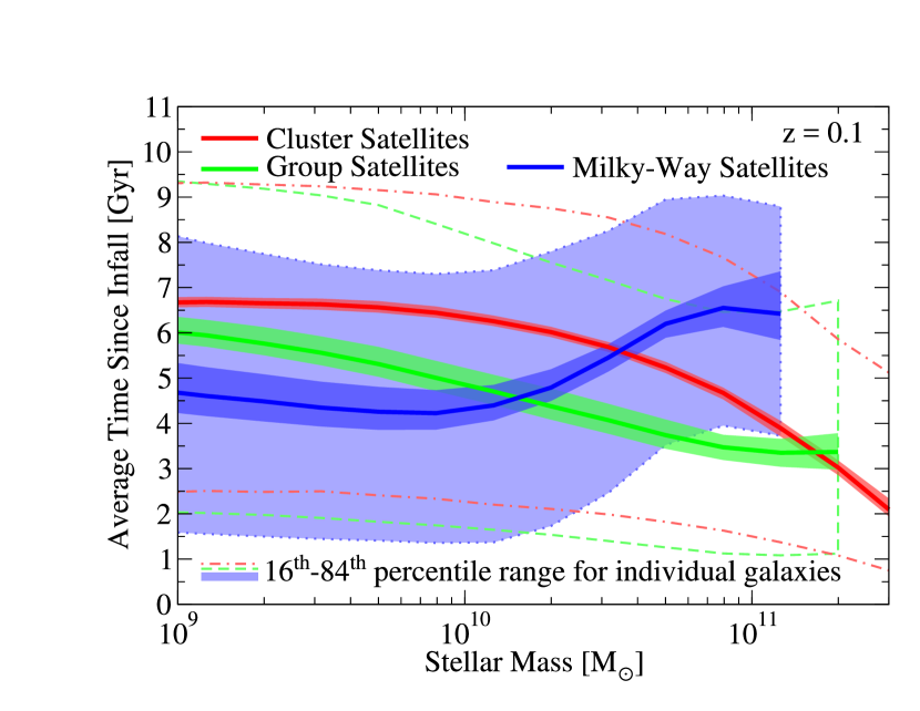
Figure 24: Left panel: the fraction of quenched $z=0$ satellite galaxies that became quenched post-infall. Solid lines show the median relation; dark shaded regions show the $16^{\mathrm{th}}-84^{\mathrm{th}}$ percentile range across the model posterior space. Right panel: the average delay times after first infall for satellite quenching (considering quenched satellites only). Solid lines show the median of the average delay time for the model posterior space; dark shaded regions show the $16^{\mathrm{th}}-84^{\mathrm{th}}$ percentile range of the average delay time across the model posterior space. The light shaded region shows the $16^{\mathrm{th}}-84^{\mathrm{th}}$ percentile range of quenching times for individual satellites of Milky-Way mass haloes; dashed and dash-dotted lines show the same for individual satellites of group and cluster-mass haloes. Notes: For all panels, Milky-Way host haloes are defined to have $11.75<\log_{10}(M_{h}/\;\mathrm{M}_{\odot})<12.25$, group-mass host haloes to have $12.75<\log_{10}(M_{h}/\;\mathrm{M}_{\odot})<13.25$, and cluster-mass host haloes to have $13.75<\log_{10}(M_{h}/\;\mathrm{M}_{\odot})<14.25$.

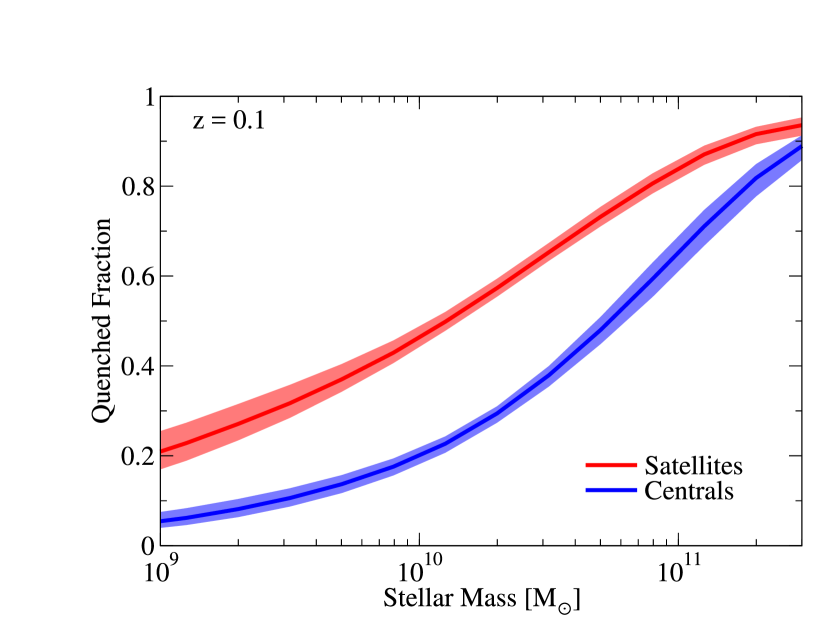
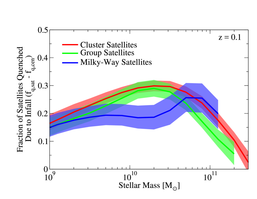
Figure 25: Left panel: average SSFRs at first infall for all $z=0$ satellite galaxies. Right panel: average time since first infall for $z=0$ satellite galaxies. Quenched Milky-way satellites have shorter average quenching delay times because there is, on average, less time since first infall. In both panels, solid lines show the median of the average value in the model posterior space and dark shaded regions show the $16^{\mathrm{th}}-84^{\mathrm{th}}$ percentile range of the average value across the model posterior space. The light shaded region shows the $16^{\mathrm{th}}-84^{\mathrm{th}}$ percentile range for individual satellites of Milky-Way mass haloes; dashed and dash-dotted lines show the same for individual satellites of group and cluster-mass haloes. As in Fig. 26, Milky-Way host haloes have $11.75<\log_{10}(M_{h}/\;\mathrm{M}_{\odot})<12.25$, group-mass host haloes have $12.75<\log_{10}(M_{h}/\;\mathrm{M}_{\odot})<13.25$, and cluster-mass host haloes have $13.75<\log_{10}(M_{h}/\;\mathrm{M}_{\odot})<14.25$.

Figure 26: Left panel: Fraction of quenched central and satellite galaxies, as a function of stellar mass. Right panel: Fraction of satellites quenched due to infall, defined as $(f_{\mathrm{q,sat}}-f_{\mathrm{q,cen}})$. In both panels, solid lines show the median relation and dark shaded regions show the $16^{\mathrm{th}}-84^{\mathrm{th}}$ percentile range across the model posterior space. As in Fig. 26, Milky-Way host haloes have $11.75<\log_{10}(M_{h}/\;\mathrm{M}_{\odot})<12.25$, group-mass host haloes have $12.75<\log_{10}(M_{h}/\;\mathrm{M}_{\odot})<13.25$, and cluster-mass host haloes have $13.75<\log_{10}(M_{h}/\;\mathrm{M}_{\odot})<14.25$.

4.4 Average Star Formation Histories

Average SFHs are shown in Fig. 17 as a function of halo mass and redshift. Quenched galaxies have lower recent SFHs and higher early SFHs, which is expected for any model that correlates quenching with assembly history. That is, lower present-day SFRs imply an earlier halo formation history, which then gives higher SFRs at early times. Central galaxies’ SFRs are more similar to satellites’ SFRs as compared to what might have been naively expected. As discussed in §4.7, star-forming satellites have similar SSFRs as star-forming central galaxies. Hence, the ratio between their average late-time SFHs is approximately the ratio of the star-forming central fraction to the star-forming satellite fraction. This ratio is never large: small haloes are mostly star-forming regardless of being centrals or satellites, and large haloes’ star-formation rates do not depend as much on assembly history (§4.6). The fact that satellite SFHs are higher on average than central SFHs is related to the fact that satellites’ peak halo masses do not grow after infall; as a result, they have more stellar mass at a given $M_{\mathrm{peak}}$ (see §4.2).

Average SFHs for galaxies are shown in Fig. 17 as a function of lookback time. Stellar populations older than $1-2$ Gyr have very similar colours (Conroy et al., 2009), so differences beyond that time are very difficult to observe. Galaxies broadly follow the same trends as haloes, with quenched galaxies and satellite galaxies having earlier formation histories than star-forming galaxies and central galaxies; the most significant differences occur within $\sim 3$ Gyr of $z=0$.

4.5 Distribution of Individual Galaxies’ Star Formation Histories

Turning to individual halo histories reveals tremendous diversity, as shown in Fig. 18. The significantly overlapping total star formation histories for $M_{h}>10^{12}\;\mathrm{M}_{\odot}$ suggest that the $z=0$ halo mass alone gives limited information on the galaxy’s recent star formation history ($z<1$). The halo mass is instead a better predictor of when the galaxy’s star formation rates peaked, as well as their early star formation history—i.e., at times when the progenitors had masses less than $10^{12}\;\mathrm{M}_{\odot}$. This is partially because it is observationally difficult to constrain SFRs in quenched galaxies, and partially because significant fractions of galaxy growth in $M_{h}>10^{12}\;\mathrm{M}_{\odot}$ haloes are from mergers (§4.8), so that contrast between their histories is diminished.

For SSFR histories (Fig. 18, middle-left panel), the $z=0$ halo mass strongly influences the range of redshifts over which quenching takes place. As noted in §4.3, $10^{13}\;\mathrm{M}_{\odot}$ haloes experience quenching over a very extended period of time, leading to more opportunities for rejuvenation. Quenching in $10^{12}\;\mathrm{M}_{\odot}$ and smaller haloes only began recently ($z<0.5$) for the majority of galaxies.

Halo mass is a much better predictor of intrahalo light (IHL) histories as compared to stellar mass histories (Fig. 18, middle-right and top-right panels). IHL depends only on mergers, which are significantly more scale-free than the process of galaxy formation (Fakhouri et al., 2010; Behroozi et al., 2013c). That said, since central galaxy stellar masses increase with dark matter halo mass, one dex increase in halo mass results in more than one dex increase in IHL; this is especially evident for low-mass haloes where the stellar mass — halo mass (SMHM) relation’s slope is greatest (§4.2).

We find broad scatter in the stellar haloes of low-mass haloes, with $\sigma_{IHL/M_{\ast}}\sim 0.6$ dex for $10^{12}\;\mathrm{M}_{\odot}$ and $\sim 1$ dex for $10^{11}\;\mathrm{M}_{\odot}$ haloes (Fig. 18, bottom panel). These are somewhat higher than predictions in Gu et al. (2016) of $\sigma_{IHL/M_{\ast}}\sim 0.38$ dex (combining 0.2 dex scatter in $M_{\ast}$ with 0.32 dex scatter in $M_{\mathrm{IHL}}$). Our inclusion of orphan galaxies (Appendix B) explains part of this difference; this choice reduces galaxy merger rates by a factor $\sim 2$, thus increasing Poisson scatter. In addition, our use of the Bernardi et al. (2013) corrections to low-redshift SMFs results in more light being associated with the central galaxy instead of the IHL. This in turn decreases the fraction of mergers that disrupt into the IHL instead of the central galaxy, explaining the rest of the increase in scatter. For massive haloes, the IHL becomes $>10\%$ of $M_{\ast}$ at $z\sim 1$. However, given that photometric surveys have only recently started capturing most of $M_{\ast}$ (Appendix C.2) at these redshifts, and given the difficulty of removing satellites (including unresolved sources) from galaxy light profiles, this is subject to the methodology employed.

Despite the diversity of stellar mass histories, galaxy progenitors adhere to well-defined SMHM relations (Fig. 18, left panel). The broadening of the scatter at early times is mostly due to halo progenitors no longer being resolved in the simulation. As in Behroozi et al. (2013e), haloes reach peak SMHM ratios when their halo masses reach $10^{12}\;\mathrm{M}_{\odot}$. Haloes that have not reached this mass at $z=0$ show increasing SMHM ratio histories, whereas those that have passed $10^{12}\;\mathrm{M}_{\odot}$ at $z=0$ show decreasing histories. The tightness of the scatter in SMHM histories depends on how well halo assembly correlates with galaxy assembly (§4.6), which is in turn constrained via star-forming vs. quenched galaxies’ correlation functions. Hence, future measurements of SSFR-split correlation functions at $z>1$ will be an important test of this model (Behroozi et al. 2019; see also §4.9).

Finally, we show derived constraints on fractional assembly times for $z=0$ galaxies in Fig. 19. We find the same general trends as Pacifici et al. (2016)—e.g., that more massive galaxies form more of their stars at early times over a shorter time period, and that star-forming galaxies have more recent assembly histories. That said, more massive galaxies in the model do have earlier formation times. This is especially apparent for massive star-forming galaxies, in which recent star formation can make it very difficult to distinguish between a very old underlying population of stars and an only moderately old population. As a result, SED-fitting techniques will sample the prior space evenly, resulting in lower average stellar ages.

4.6 Correlations between Galaxy and Halo Assembly and the Permanence of Quenching

The rank correlation between galaxy SFR and halo assembly rate ($\equiv\Delta v_{\mathrm{max}}$, Eq. 1) is significant and unequivocally detected (Fig. 20). There may also be a weak trend with halo mass. Small haloes’ SFRs are more correlated with their assembly history ($r_{c}\sim 0.6$), whereas large haloes’ SFRs may be more independent ($r_{c}\sim 0.5$). Observationally, the clearest effect of a strong halo—galaxy assembly correlation is that satellites are quenched much more often than centrals; this also causes large separations in quenched vs. star-forming galaxies’ correlation functions. Almost all quenched dwarf galaxies ($M_{\ast}<10^{9}\;\mathrm{M}_{\odot}$) are satellites (Geha et al., 2012), implying a strong assembly correlation. Yet, the relative difference in quenched fractions for centrals and satellites becomes less with increasing mass (Wetzel et al., 2012), as does the relative difference in clustering strength between quenched and star-forming galaxies (Fig. 5). Massive haloes hence plausibly have weaker correlations between galaxy SFRs and halo assembly. At the same time, galaxies in massive haloes grow mainly via mergers, so that this lower correlation does not cause increased scatter in the SMHM relation (Fig. 14).

In models where galaxy assembly correlates with halo assembly, galaxy rejuvenation (i.e., the resumption of star formation following a period of quiescence) is a generic feature (e.g., Fig. 23, right panel). Almost by definition, proxies of halo assembly change significantly over a dynamical time (e.g., from mergers, accretion, or infall into another larger halo); these changes will in turn affect galaxy SFRs. If a galaxy population’s quenched fraction changes slowly compared to halo dynamical times, changes in halo assembly rates will have the most opportunity to switch galaxies from being star-forming to quenched and vice versa. This is especially the case for galaxies in $10^{12}-10^{13}\;\mathrm{M}_{\odot}$ haloes, which quench at a rate of $<10\%$ per dynamical time (Fig. 17, right panel; see also Fig. 18, middle-left panel). More massive haloes become fully quenched too rapidly, and less-massive haloes never have large enough quenched fractions for rejuvenation to be as common.

We find exactly this behaviour arising in the models (Fig. 23). Here, we define rejuvenation as at least $300$ Myr of quiescence, followed by at least 300 Myr of star formation; this prevents brief spikes of quiescence (as in the black curve at $t=5$Gyr in Fig. 23, right panel) or star formation from counting as a rejuvenation event. The majority of $10^{12}-10^{13}\;\mathrm{M}_{\odot}$ haloes at $z=0$ experienced at least one rejuvenation event in their past. This fraction falls significantly for both higher and lower halo masses, as well as at $z\geq 1$ when galaxy quenched fractions were significantly lower. Unfortunately, this behaviour is difficult to observe in integrated colours or spectra. Rejuvenated galaxies at $z=0$ typically spent $\sim 1$ Gyr forming stars since their last quiescent period (Fig. 23, left panel), which typically lasted $\sim 2$ Gyr. The brightness of young stars and the similarity in colours of $2$ Gyr vs. $4$ Gyr stellar populations thus make this very difficult to detect. Timescales at $z=1$ are somewhat more amenable to observations (Fig. 23, right panel), perhaps with LEGA-C (van der Wel et al., 2016), although a much smaller fraction of galaxies at that cosmic time had been rejuvenated (Fig. 23).

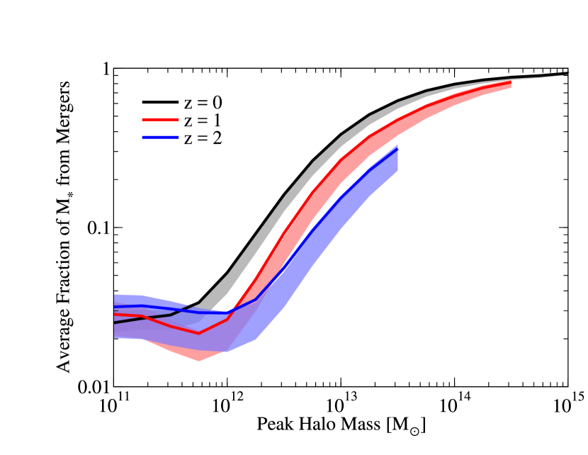
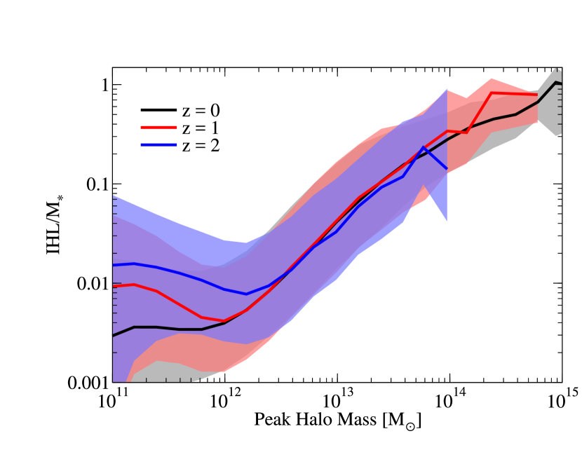
Figure 27: Left panel: average fraction of galaxy mass that was formed ex-situ—i.e., that came in via mergers. Shaded regions show the 68% confidence interval from the model posterior distribution. Right panel: median ratio of stellar mass in the intrahalo light (IHL) to $M_{\ast}$. Shaded regions show the $16^{\mathrm{th}}-84^{\mathrm{th}}$ percentile range for individual galaxies in the best-fitting model. Notes: the Bolshoi-Planck simulation resolves haloes down to $10^{10}\;\mathrm{M}_{\odot}$, with the result that mergers are well-resolved for haloes down to $10^{11}\;\mathrm{M}_{\odot}$. Including mergers from haloes with $M_{h}<10^{10}\;\mathrm{M}_{\odot}$ would contribute negligibly to ex-situ and IHL fractions due to the steepness of the SMHM relation (Fig. 11).

4.7 The Fate of Satellite Galaxies Post-Infall

Except for massive galaxies, most quenched satellites at $z=0$ became quenched after infall into a larger halo (Fig. 26, left panel). Past investigations of satellite quenching (e.g., Wetzel et al., 2013; Wetzel et al., 2015; Wheeler et al., 2014; Oman & Hudson, 2016) assumed that all satellites quench after the same delay time following infall. We find the same basic trends as these previous works (Fig. 26, right panel); low-mass galaxies quench on average much longer after infall than high-mass galaxies, and there is little dependence on delay timescales with host halo mass for $M_{\mathrm{host}}>10^{13}\;\mathrm{M}_{\odot}$.

A key assumption of the uniform time delay models is that satellites quench in order of infall time. This is not true for the model and presumably the real Universe as well, as satellites arrive at their host haloes with a wide variety of SSFRs (Fig. 26, left panel). Some are on the verge of quenching, and so quench rapidly after infall, whereas some remain on the star-forming main sequence until $z=0$. In addition, satellites have a wide variety of post-infall trajectories: some satellites on very radial orbits are stripped and quenched very quickly, whereas others remain on more circular orbits and experience much less disruption. This results in the broad distribution of quenching time delays we find (Fig. 26, right panel), and also introduces a correlation between the average quenching time delay and the average infall time. For example, as satellites in Milky Way-like hosts ($M_{\mathrm{host}}\sim 10^{12}\;\mathrm{M}_{\odot}$) had later average infall times (Fig. 26, right panel), a smaller fraction of the satellites that will eventually quench had time to do so by $z=0$. As a result, average delay times for quenched galaxies in these haloes are systematically lower than those inferred by uniform delay time models.

Delay time models often implicitly assume that post-infall quenching is entirely due to interactions with the host halo. Being a satellite certainly results in a higher probability of being quenched (Fig. 26, left panel). However, central galaxies are also quenching at the same time. Just as a “quenching delay time” is meaningless for a central galaxy, it is meaningless for the large fraction of satellite galaxies that would have quenched even if they had been in the field. Indeed, for galaxies with $M_{\ast}>10^{10.5}\;\mathrm{M}_{\odot}$, the majority of quenched $z=0$ satellites would have quenched without any host interactions (Fig. 26, left panel). Considering the excess quenched fraction of satellites in absolute terms ($f_{\mathrm{q,sat}}(M_{\ast})-f_{\mathrm{q,cen}}(M_{\ast})$), we find that this never exceeds 30% (Fig. 26, right panel), similar to past results (Wetzel et al., 2012; Wang et al., 2018). Regardless of how one then defines “quenching due to infall,” this result suggests that it does not happen to most satellites. As discussed in §5.3, cluster images typically show only the most visually interesting inner regions (where most satellites are quenched) instead of the outskirts (where many satellites are still star-forming), leading to the common misperception that most satellites are quenched.

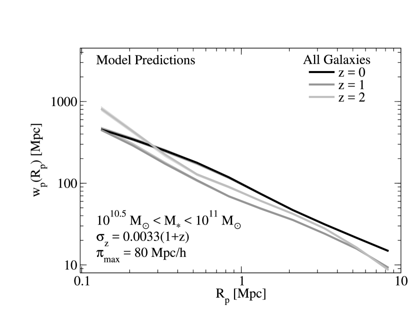
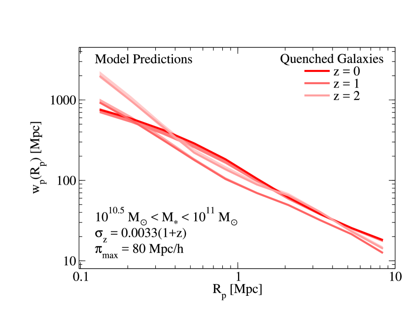
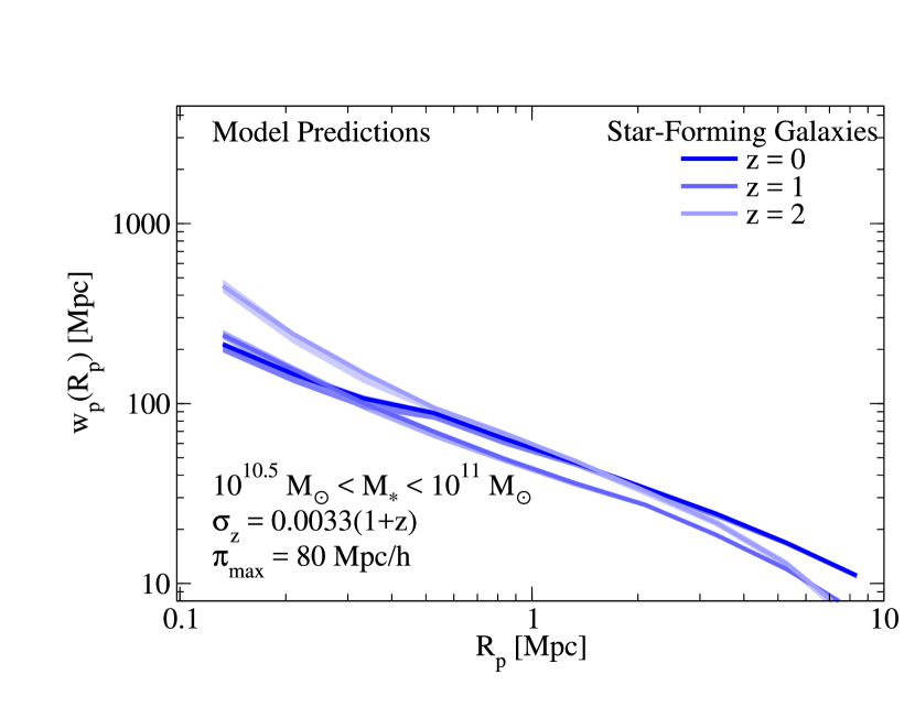
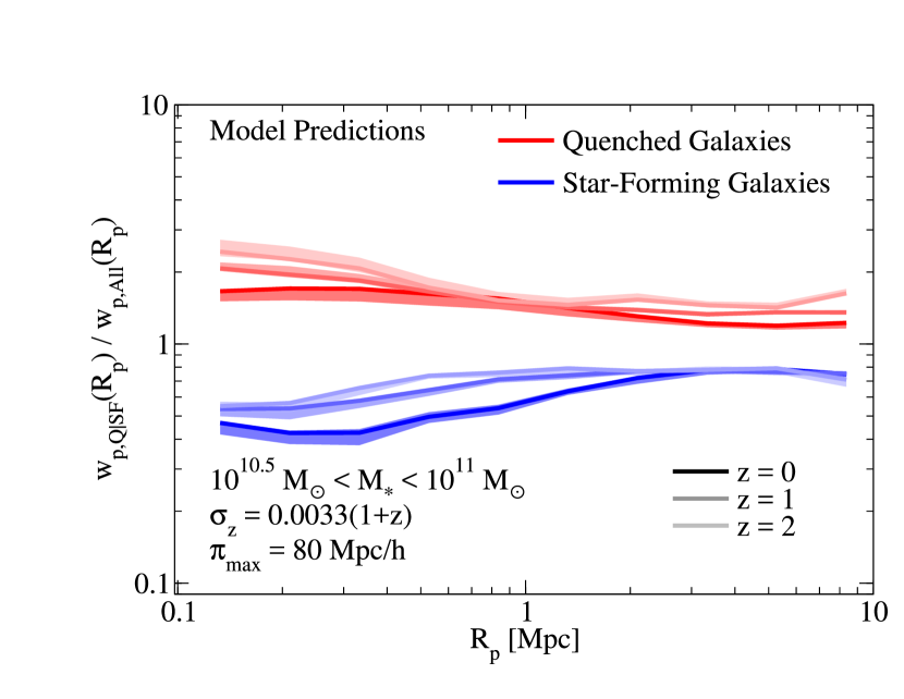
Figure 28: Top-left panel: predictions for galaxy autocorrelation functions at $z>0$, assuming line-of-sight integration to $\pi_{\mathrm{max}}=80$ Mpc $h^{-1}$ and redshift errors of $\sigma_{z}/(1+z)=0.0033$, similar to the PRIMUS survey (see Appendix C.7). Top-right and Bottom-left panels: same as top-left panel for quenched ($SSFR<10^{-11}$ yr^-1) and star-forming galaxies, respectively. Bottom-right panel: the ratio of $w_{p}(R_{p})$ for quenched and star-forming galaxies to $w_{p}(R_{p})$ for all galaxies. Shaded regions show the $16^{\mathrm{th}}-84^{\mathrm{th}}$ percentile range of the model posterior distribution. All distances are in comoving units. Predictions for other mass ranges available online.

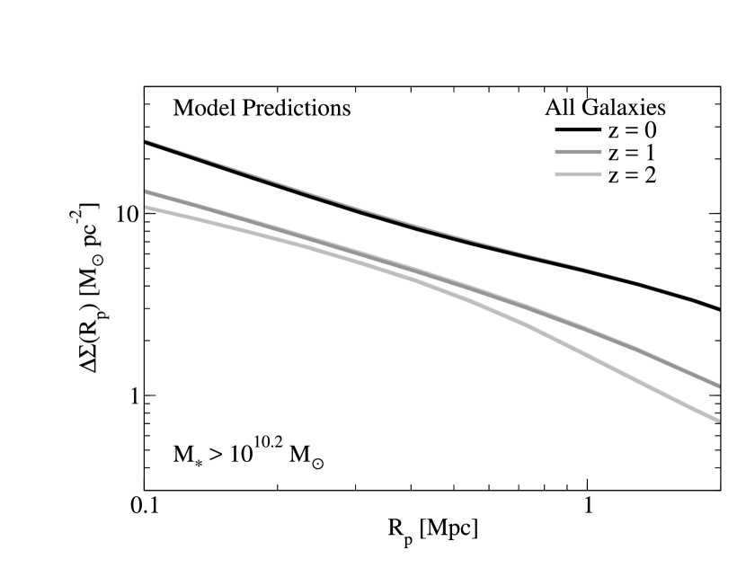
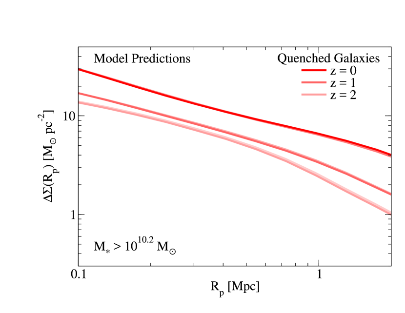
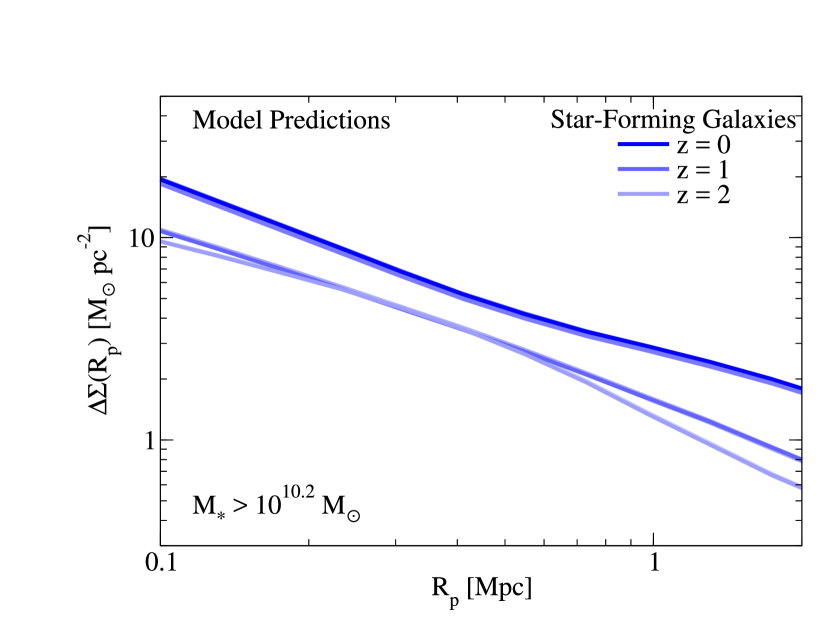
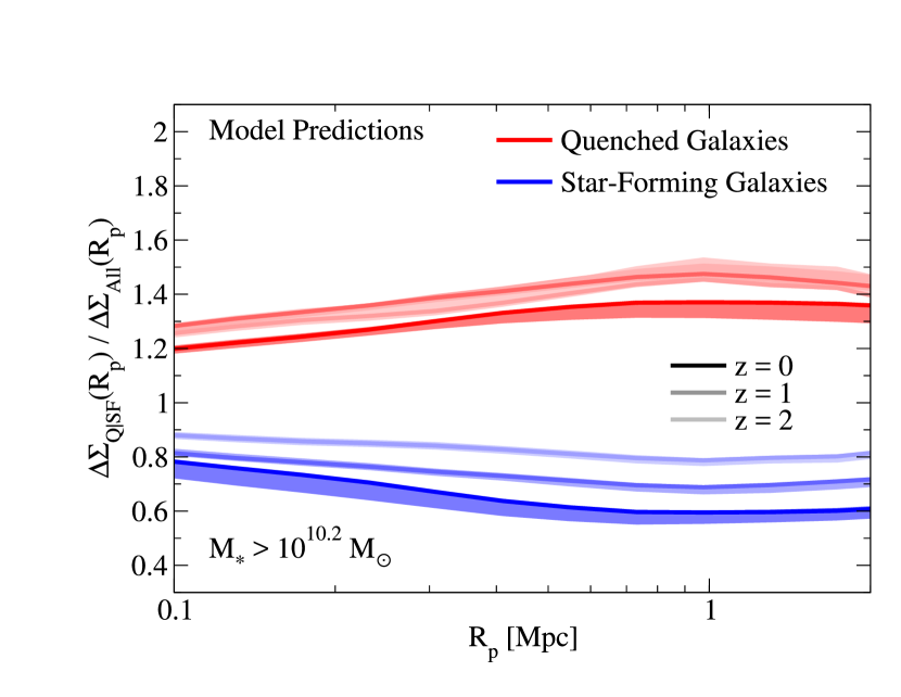
Figure 29: Top-left panel: predictions for excess surface densities ($\Delta\Sigma$) for all galaxies with $M_{\ast}>10^{10.2}\;\mathrm{M}_{\odot}$ as probed by galaxy-galaxy lensing at $z>0$. Top-right and Bottom-left panels: same as top-left panel for quenched ($SSFR<10^{-11}$ yr^-1) and star-forming galaxies, respectively. Bottom-right panel: the ratio of $\Delta\Sigma$ for quenched and star-forming galaxies to that for all galaxies. Shaded regions show the $16^{\mathrm{th}}-84^{\mathrm{th}}$ percentile range of the model posterior distribution. All distances are in comoving units. Predictions for other mass ranges available online.

4.8 Fraction of Stellar Mass from In-Situ vs. Ex-Situ Growth

The fraction of stellar mass from ex-situ vs. in-situ star-formation increases with increasing halo mass and decreasing redshift (Fig. 27, left panel). As massive galaxies are mostly quenched (Fig. 4, right panel), their only channel for growth comes via mergers of smaller haloes. However, because of the shape of the SMHM relation (Fig. 11), haloes with $M_{h}<10^{12}\;\mathrm{M}_{\odot}$ have strongly decreasing stellar fractions towards lower masses. As a result, mass growth via mergers is only efficient for haloes with $M_{h}>10^{12}\;\mathrm{M}_{\odot}$. This is also reflected in the intrahalo light (IHL) to $M_{\ast}$ ratio (Fig. 27, right panel). We find that the IHL / $M_{\ast}$ ratio reaches $\sim 0.3$ at halo masses of $10^{14}\;\mathrm{M}_{\odot}$ at $z=0$. This is $\sim 0.5$ dex lower than past results (e.g. Gonzalez et al., 2007; Moster et al., 2013; Behroozi et al., 2013e), as the SMFs used in this study assign more light to the central galaxy that previously would have been assigned to the IHL (Bernardi et al., 2013; Kravtsov et al., 2018). Direct comparison with Behroozi et al. (2013e) is available online.

4.9 Predictions for Galaxies’ Autocorrelation and Weak Lensing Statistics

Fig. 28 shows predictions for a hypothetical PRIMUS-like survey extending to $z=2$. At fixed galaxy mass, the overall clustering signal decreases from $z=0$ to $z=1$ partially due to reduced satellite fractions at higher redshifts. The clustering signal increases again from $z=1$ to $z=2$ due to the increased rarity (and hence bias) of the host haloes. As the quenched fraction decreases with increasing redshift, quenched galaxies have increasingly larger offsets relative to the all-galaxy correlation function (Fig. 28, bottom-right panel). That is, being quenched at higher redshifts requires increasingly extreme accretion histories, resulting in only the most stripped (and therefore clustered) haloes at high redshift being quenched. Similarly, star-forming galaxy correlation functions also increase relative to the all-galaxy correlation function with increasing redshift.

We generate weak lensing predictions via projected dark matter surface densities in Bolshoi-Planck. Surface densities are integrated along the full extent (250 Mpc h^-1) of the $z$-axis in projected radial bins around each halo. Given the surface density $\Sigma(r_{p})$, we compute the excess surface density $\Delta\Sigma$:

$$\Delta\Sigma(r_{p})\equiv\frac{\int_{0}^{r_{p}}\Sigma(r)\pi rdr}{\pi r_{p}^{2}}-\Sigma(r_{p}).$$ (30)

Fig. 29 shows the resulting predictions; see Hearin et al. (2014) for a discussion of the limitations of this approach. Similar to autocorrelation functions, the lensing signal decreases from $z=0$ to $z=1$, partially due to lower satellite fractions, and partially due to lower halo concentrations (Diemer et al., 2013; Diemer & Kravtsov, 2015; Rodríguez-Puebla et al., 2016b). The latter is especially evident at halo outskirts. The same factors continue to affect the lensing signal at higher redshifts; hence, the lensing signal continues to decrease in contrast to the galaxy autocorrelation signal. Combined with a decreasing number density of lens sources at higher redshifts, this suggests that clustering will offer better halo mass constraints than lensing at high redshifts. Predictions for clustering at $z>2$ relevant to the James Webb Space Telescope are presented in R. Endsley, et al. (in prep.).

4.10 Systematic Uncertainties

Stellar masses have many systematic uncertainties, including the stellar population synthesis model, dust, metallicities, and star formation histories assumed (Conroy et al., 2009; Conroy & Gunn, 2010; Behroozi et al., 2010). Empirical models allow self-consistently treating uncertainties in dust (e.g., Imara et al., 2018), metallicity (e.g., Lu et al., 2015a, c), and star formation histories (e.g., Moster et al., 2013, 2018; Behroozi et al., 2013e) when fitting to multi-band luminosity functions, potentially removing many of these systematic uncertainties. The current model is a first step in this direction, despite the simplicity of the dust model assumed and the lack of non-UV luminosity functions. A comparison between specific SFRs and stellar mass function evolution reveals strong inconsistencies between observations that would be resolved by $0.3$ dex higher stellar masses (or 0.3 dex lower SFRs) at $z=2$ (Appendix C.4). Regardless, our inferred “true” stellar masses and star formation rates are always within $0.3$ dex of the observed values (e.g., Fig. 4, left panel).

4.11 Additional Data Available Online

The online data release includes underlying data and documentation for all the figures in this paper, as well as additional mass and redshift ranges where applicable, as well as model posterior uncertainties where possible. The data release also includes halo and galaxy catalogues for the best-fitting model applied to the Bolshoi-Planck simulation (both in text format and in an easily-accessible binary format integrated with HaloTools; Hearin et al. 2017), full star formation and mass assembly histories for haloes at $z=0,1$ and $2$, and mock lightcones corresponding to the five CANDELS fields (Grogin et al., 2011). The data release includes a snapshot of the UniverseMachine code (Appendix F) that was used for this paper.

5 Discussion

We discuss how results in §4 impact connections between galaxy and halo assembly (§5.1), central (§5.2) and satellite (§5.3) quenching, tracing galaxies across cosmic time (§5.4), equilibrium/bathtub models of galaxy formation (§5.5), “impossibly early” galaxies (§5.6), uniqueness of the model (§5.7), and orphan galaxies (§5.8); we also compare to previous results (§39) and discuss evolution in the stellar mass–halo mass relation (§5.10). We discuss how additional observations and modeling could address current assumptions and uncertainties (§5.11), and finish with future directions for empirical modeling (§5.12).

5.1 Connections Between Individual Galaxy and Halo Assembly

We find that star-forming galaxies reside in significantly more rapidly-accreting haloes than quiescent galaxies (§4.6). This is especially clear for satellites, which drive differences in autocorrelation functions between quenched and star-forming galaxies (Fig. 5). It is also clear for “backsplash” galaxies–i.e., those that passed inside a larger host’s virial radius before exiting again; these drive the environmental dependence of the quenched fraction for central galaxies (Fig. 8).

Correlation constraints are much weaker for central galaxies that never interacted with a larger halo. Indeed, Tinker et al. (2011); Tinker et al. (2017) argue that no correlations exist between low-mass galaxy assembly and quenching except for satellite and backsplash galaxies (as in Peng et al., 2010, 2012). That said, their main evidence is that star-forming fractions for central galaxies seem not to depend on environmental density except for the highest-density environments. As shown in Fig. 8, the model herein has no problem matching this behaviour even with a fairly strong quenching-assembly correlation, similar to the finding in Wang et al. (2018); this is due to the fact that assembly histories do not change significantly for haloes in low- vs.  median-density environments (Lee et al., 2017). Behroozi et al. (2015a) argues that enhanced mass accretion during major mergers does not correlate with galaxy quenching at $z=0$; however, this does not preclude a correlation with smooth accretion. Determining correlations between smooth matter accretion rates and galaxy formation will require alternate techniques to measure halo mass accretion rates, such as splashback radii (e.g., More et al., 2016).

If quenching does correlate with assembly history for isolated centrals, then it becomes very difficult to avoid rejuvenation (§4.6) in $10^{11}\;\mathrm{M}_{\odot}$ galaxies. This is because such galaxies’ quenched fractions increased slowly over many halo dynamical times—so that changes in assembly history occurred much more rapidly than changes in the quenched fraction. Thus, the number of such galaxies that quench at any given time due to recently low or negative accretion rates must be approximately balanced by the number that rejuvenate due to recently high accretion rates. Avoiding this is possible only if central galaxy quenching is not significantly correlated with halo assembly. As a result, the depth of the green valley in colour space represents another way to test quenching models, as multiple passes through the green valley will lead to a shallower valley than models where galaxies quench only once.

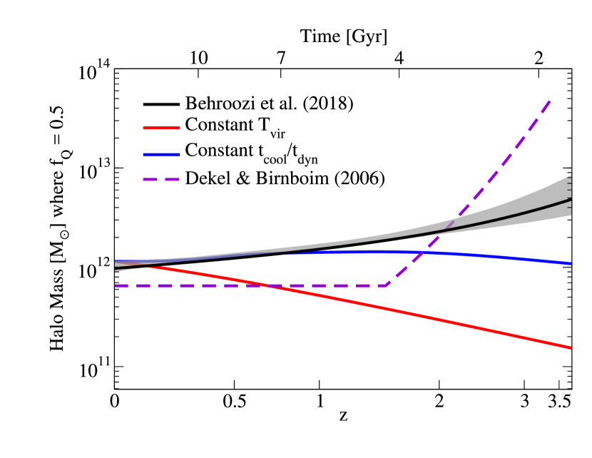
Figure 30: Empirical halo mass quenching thresholds from this work (black line; defined as the halo mass at which $50\%$ of galaxies are quenched) compared to theoretical cooling-based thresholds. The red line shows a model where quenching occurs above a virial temperature threshold of 6.4$\times 10^{5}$K; the blue line shows a model where quenching occurs if the cooling/dynamical time ratio $t_{\mathrm{cool}}/t_{\mathrm{dyn}}$ is greater than $0.4$. The purple dashed line shows the model of Dekel & Birnboim (2006). The grey shaded region shows the $16^{\mathrm{th}}-84^{\mathrm{th}}$ percentile range from the posterior distribution for this work. Notes: see text for definition of $t_{\mathrm{cool}}$ and $t_{\mathrm{dyn}}$.

5.2 Central Galaxy Quenching

At fixed halo mass, we find that the galaxy quenched fraction decreases with increasing redshift (§4.3). This is a robust conclusion in other empirical models (e.g., Moster et al., 2018), due to the decreasing galaxy quenched fraction at fixed stellar mass (e.g., Muzzin et al., 2013) and the constancy of the stellar mass–halo mass relation from $z=4$ to $z=0$ (Behroozi et al., 2013c). Vice versa, as shown in Fig. 30, the halo mass at which a fixed fraction of galaxies are quenched (e.g., 50%) increases with increasing redshift.

This latter fact implies that a virial temperature threshold alone is not responsible for quenching. Virial temperatures increase with redshift at fixed halo mass, so a constant virial temperature quenching threshold would predict that the threshold halo mass for quenching should decrease with increasing redshift (Fig. 30). A similar argument applies to thresholds in the ratio of the cooling time to the halo dynamical time (or the free-fall time or the age of the Universe, which are proportional). These typically give redshift-independent quenched fractions with halo mass (see Fig. 8.6 in Mo et al., 2010). Here, we adopt a crude cooling time estimate from Mo et al. (2010):

$$t_{\mathrm{cool}}\sim 1.5\times 10^{9}\;\mathrm{yr}\;\left(\frac{T_{\mathrm{vir}}}{10^{6}\;\mathrm{K}}\right)\left(\frac{10^{-3}\;\mathrm{cm}^{-3}}{\langle n_{H}\rangle}\right)\left(\frac{10^{-23}\;\mathrm{erg}\;\mathrm{cm}^{3}\;\mathrm{s}^{-1}}{\Lambda(T_{\mathrm{vir}})}\right),$$ (31)

where $n_{H}$ is the average density of hydrogen atoms in the halo; we take the cooling function $\Lambda(T)$ from De Rijcke et al. (2013) for a $1/3Z_{\odot}$ gas. For the halo dynamical time, we define as before $t_{\mathrm{dyn}}\equiv(\frac{4}{3}\pi G\rho_{\mathrm{vir}})^{-\frac{1}{2}}$. As shown in Fig. 30, a model where haloes quench above a constant $t_{\mathrm{cool}}/t_{\mathrm{dyn}}$ threshold may be plausible from $z=0$ to $z=1$, but this model is inconsistent with our results at $z>1$.

Dekel & Birnboim (2006) posit that at higher redshifts, cold streams can more effectively penetrate hot haloes ($M_{h}>10^{12}\;\mathrm{M}_{\odot}$), allowing for residual star formation. As shown in Fig. 30, our best-fitting model allows gradually more residual star formation in hot haloes with increasing redshift. Yet, Dekel & Birnboim (2006) predicted a steeper transition for cold streams to exist in hot haloes at redshifts $z>1.5-2$ than we find here, suggesting that the quantitative details of quenching are different. Indeed, this is expected at a basic level because Dekel & Birnboim (2006) do not discuss the effect of black holes, which are also expected to play a role in quenching (e.g., Silk & Rees, 1998).

Isolated central haloes (as opposed to backsplash haloes) rarely lose matter, and so their quenching in this model is driven by recent mergers and random internal processes. During a merger, the maximum circular velocity ($v_{\mathrm{max}}$) will rapidly increase during first passage, resulting in a burst of star formation; $v_{\mathrm{max}}$ then rapidly decreases as kinetic energy from the merger dissipates into increased halo velocity dispersion and lower halo concentration (Behroozi et al., 2014a). In the latter phase, the galaxy will be quenched in our model, resulting in a post-starburst galaxy. As the quenched fraction decreases toward higher redshifts, only the most extreme merging events will result in quenched centrals, meaning that the fraction of quenched non-satellite galaxies that are post-starburst will increase with redshift. We hesitate to call this a prediction, since a different equally-reasonable choice of halo assembly proxy may have different behaviour; instead, it is a testable hypothesis.

5.3 Satellite Galaxy Quenching

For satellites, many quenching mechanisms have been proposed, including ram-pressure/tidal stripping (Gunn & Gott, 1972; Byrd & Valtonen, 1990), strangulation (Larson et al., 1980), accretion shocks (Dressler & Gunn, 1983), and harassment from other satellites (Farouki & Shapiro, 1981), among others. Given the diversity of satellite orbits and infall conditions, it is likely that all of these mechanisms each quench some fraction of satellites. For example, extremely high fractions of quenched galaxies in cluster centers (Wetzel et al., 2012) may suggest that galaxies quench rapidly there. That said, we find that satellite quenching is neither efficient nor necessarily a rapid process for most satellites (§4.7), suggesting that accretion shocks may not be dominant. In addition, harassment from other satellites is problematic because high velocities inside clusters mean that strong interactions are less likely to occur (Binney & Tremaine, 2008). This suggests that inefficient ram-pressure/tidal stripping (e.g., Emerick et al., 2016) coupled with strangulation is sufficient to explain most satellite quenching (see also Balogh et al., 2016; Fillingham et al., 2018). In addition, feedback models that launch galaxy gas to significant fractions of the virial radius (leading to efficient stripping) will generically overproduce satellite galaxy quenched fractions.

5.4 Tracing Galaxies Back in Time

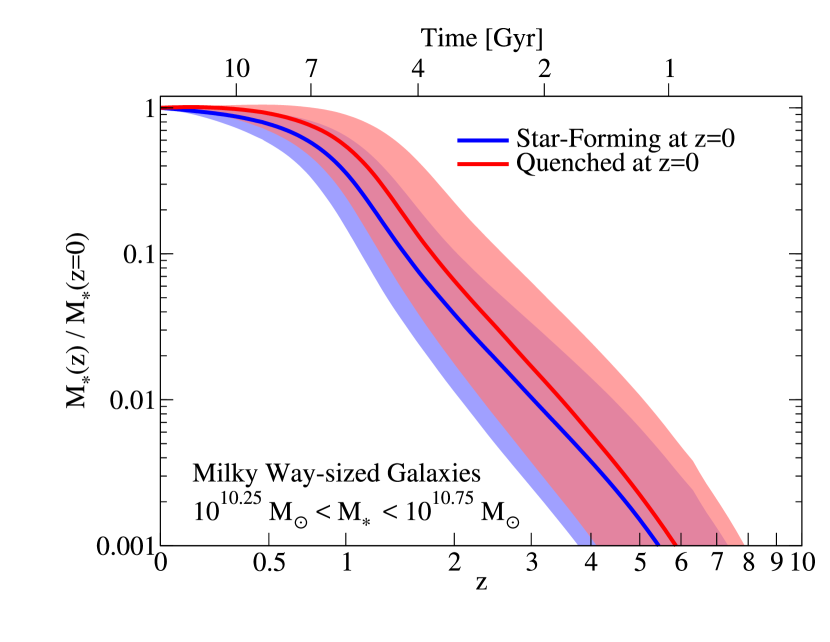
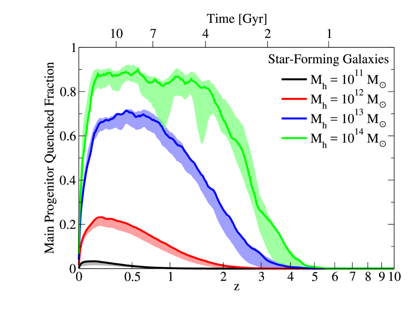
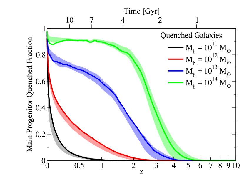
Figure 31: Top panel: stellar mass histories for star-forming and quenched galaxies at $\sim$Milky-Way masses. Middle panel: for star-forming galaxies at $z=0$, the fraction of their main progenitors that are quenched as a function of redshift. By definition, this fraction is 0 at $z=0$. Bottom panel: same, for quenched galaxies at $z=0$; by definition, the fraction is 1 at $z=0$. Differences between main progenitor quenched fractions for $z=0$ quenched and star-forming galaxies largely disappear by $z=0.5$.

Using cumulative number densities to follow galaxy progenitors (e.g., Leja et al., 2013; van Dokkum et al., 2013; Lin et al., 2013) has become an increasingly popular approach despite the large scatter in progenitor histories (Behroozi et al., 2013f; Torrey et al., 2017; Jaacks et al., 2016; Wellons & Torrey, 2017). Recently, Clauwens et al. (2016) noted differences between median progenitor histories for star-forming and quenched galaxies in the EAGLE simulation (Schaye et al., 2015). In our best-fitting model, we also find such differences (Fig. 31, top panel), but find as in Clauwens et al. (2016) that the scatter in individual progenitor histories dwarfs the median difference at all redshifts. Joint selection on cumulative number density and SSFR will be explored in future work. Most of the power in differentiating galaxy properties may only come over galaxies’ recent histories; e.g., the difference in progenitor star-forming fractions between quenched and star-forming galaxies largely disappears by $z=0.5$ (Fig. 31, middle and bottom panels).

5.5 Equilibrium vs. Non-Equilibrium Models

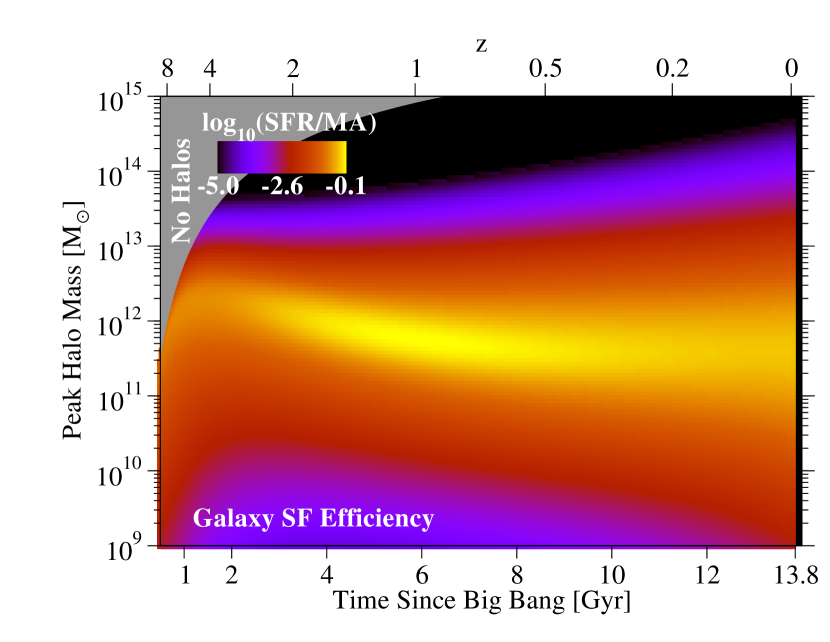
Figure 32: Average galaxy star formation efficiency, defined as the ratio of average galaxy SFR to the average baryonic mass accretion rate of the host dark matter halo. This is shown as a function of cosmic time and peak halo mass (at the given cosmic time, as opposed to $z=0$). The baryonic mass accretion rate is approximated as $f_{b}\dot{M}_{h}$, where $f_{b}=0.16$ is the cosmic baryon fraction. Compare to analogous figure in Behroozi et al. (2013c) online. Notes: relative uncertainties are the same as for average galaxy SFRs, shown in Fig. 14, left panel.

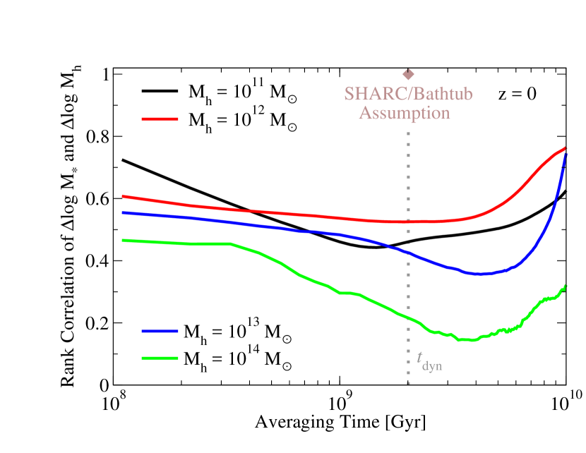
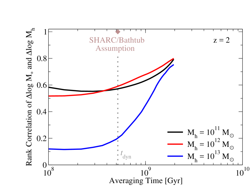
Figure 33: Top panel: rank correlation of average galaxy specific growth rate ($\langle\frac{d\log{M_{\ast}}}{dt}\rangle$) to average specific halo mass accretion rate ($\langle\frac{d\log{M_{\mathrm{peak}}}}{dt}\rangle$) as a function of averaging time at $z=0$ for the best-fitting model. Also shown for comparison is the Stellar-Halo Accretion Rate Coevolution (SHARC) assumption from Rodríguez-Puebla et al. (2016a), corresponding to a rank correlation of 1 for averaging over a dynamical time. Bottom panel: Same, at $z=2$. In both panels, the grey dotted line denotes the dynamical time at the given redshift.

In equilibrium (a.k.a., “steady-state” or “bathtub”) models of galaxy formation (e.g., Bouché et al., 2010; Davé et al., 2010; Lilly et al., 2013), galaxies form stars according to average gas accretion rates scaled by a mass-dependent efficiency. Observational evidence that galaxies behave in this way on average (e.g. Behroozi et al., 2013c) gave rise to empirical models in which individual galaxies’ SFRs are linearly related to halo gas accretion rates (Becker, 2015; Rodríguez-Puebla et al., 2016a; Sun & Furlanetto, 2016; Mitra et al., 2017; Cohn, 2017; Moster et al., 2018). In principle, the average behaviour could also be reproduced if individual galaxies’ positions varied randomly on the SSFR main sequence, with no relation to mass accretion rates. At $z=0$, two lines of evidence are inconsistent with linear relationships between mass accretion rates and star formation rates; specifically, star-forming satellites’ SSFRs are not offset significantly from star-forming centrals’ SSFRs (Wetzel et al., 2012), and major halo mergers do not result in enhanced star-forming fractions or enhanced SFRs for star-forming galaxies (Behroozi et al., 2015a).

The model in this paper reproduces an average ratio between gas accretion and star formation that is nearly constant in time (Fig. 32), using a strong but imperfect correlation between galaxy assembly and halo assembly ($\sim 0.5-0.6$; §4.6). If indeed main-sequence SSFRs were perfectly correlated with assembly history at $z\sim 0$, it would be very difficult for satellite fractions to be large enough to explain the autocorrelation function for galaxies; we also find that star-forming central galaxies’ SSFRs do not depend much on environment density (Appendix C.8; see also Berti et al. 2017), whereas central halo accretion rates are known to do so (Lee et al., 2017).

We note that even for models where SFR depends only on halo mass and cosmic time (i.e., not on assembly history), long-term correlations between halo and galaxy growth can result. Because SFR rises steeply with halo mass for $M_{h}<10^{12}\;\mathrm{M}_{\odot}$, a larger growth in halo mass will guarantee a larger change in SFRs and therefore in $M_{\ast}$. On the other hand, mergers can reduce correlations between stellar mass growth and halo mass growth due to the shape of the SMHM relation; this is especially true for massive haloes. The combination of mergers and induced SFR–halo growth correlations results in a very nontrivial shape for how overall galaxy growth—halo growth correlations depend on the averaging timescale (Fig. 33).

5.6 “Impossibly” Early Galaxies

Steinhardt et al. (2016) recently found that $z>4$ galaxy number densities are too large to reconcile with $\Lambda$CDM dark matter halo number densities unless certain conditions are met. Of these conditions, we find that it is sufficient for stellar fractions in dark matter haloes to increase with increasing redshift (§39; see also Jaacks et al. 2012a; Liu et al. 2016; Behroozi & Silk 2015, 2018). The best-fitting model matches both observed stellar mass functions (Fig. 4) and UV luminosity functions (Fig. 4) at $z>4$, using reasonable stellar fractions (Fig. 11), dust attenuation (Fig. 8), and stellar population synthesis models (FSPS; Conroy et al., 2009). Thus, we do not find the observed $z>4$ number densities to be a cause for concern with $\Lambda$CDM.

5.7 Uniqueness

With one-point statistics (SMFs, SFRs, and quenched fractions) alone, there are many mathematically-allowed solutions for galaxies’ star formation histories (e.g., Gladders et al., 2013; Kelson, 2014; Abramson et al., 2015, 2016). This arises because individual galaxies’ long-term star-formation histories are not directly measured by such statistics, requiring an additional constraint. Our method relies on $z<1$ clustering and environmental constraints to anchor the relationship between galaxies and haloes. As haloes’ growth histories are well-measured (Srisawat et al., 2013), the uniqueness of the solution is set by the tightness of the galaxy—halo relationship, implying that long-term stellar mass growth histories can be inferred to within $\sim$0.3 dex (Fig. 18, top-right panel) if the halo mass is known. Matching the $z>1$ stellar mass–halo mass relation from independent clustering measurements (§39) is thus a nontrivial prediction that favours model uniqueness.

That said, constraining recent SFR histories is challenging even if the halo mass is known (Fig. 18, top-left panel). This is especially true at $z<2$, where halo mass has little predictive power for galaxy SFRs for $M_{h}>10^{12}\;\mathrm{M}_{\odot}$ galaxies (see also Behroozi et al., 2013e). Knowledge of halo growth rates does appear to help (Figs. 20 and 33), but less so for the most massive galaxies. Physically, this is consistent with more stochastic star formation in massive galaxies at late times (e.g., due to fluctuating activity in the central black hole), but more predictable (i.e., more constrainable) star formation in lower-mass galaxies and at early times.

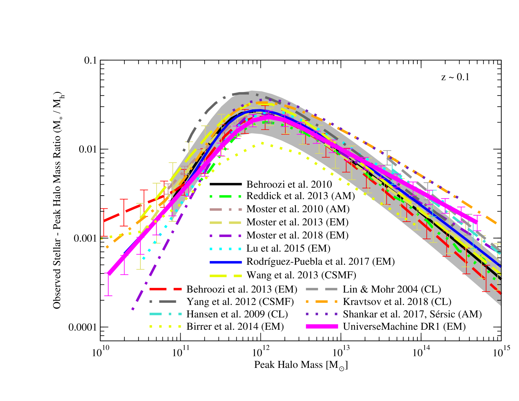
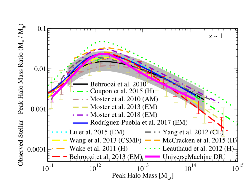
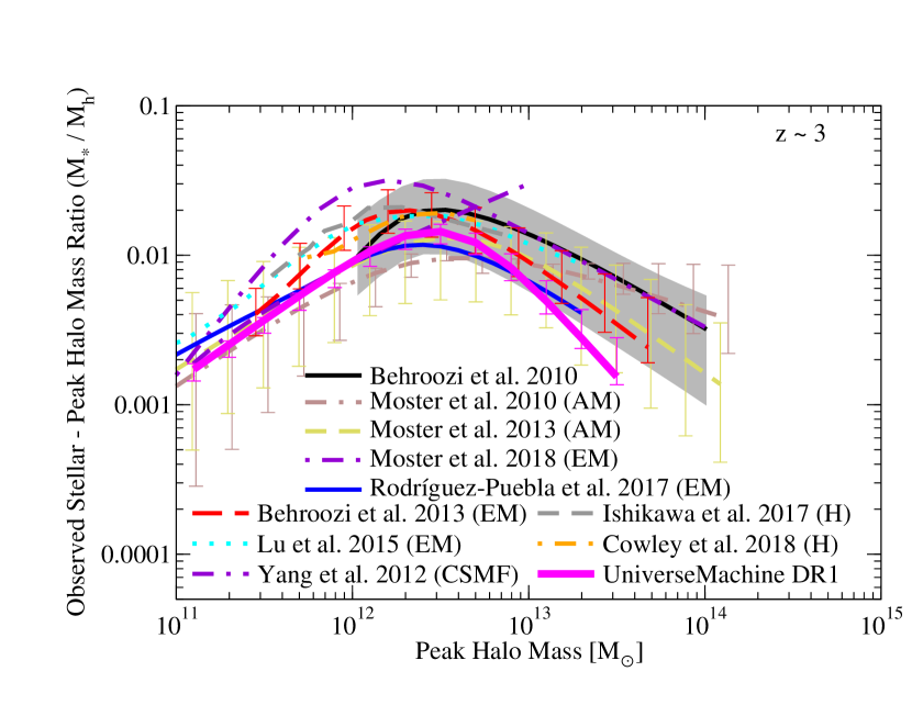
Figure 34: Median observed stellar mass — halo mass relation for our best-fitting model (labelled as “UniverseMachine DR1”) compared to previous results at $z=0.1$. Results compared include those from our previous works (Behroozi et al., 2010, 2013e), from empirical modeling (EM; Moster et al., 2013, 2018; Birrer et al., 2014; Lu et al., 2015b; Rodríguez-Puebla et al., 2017), from abundance matching (AM; Moster et al., 2010; Reddick et al., 2013; Shankar et al., 2017), from Conditional Stellar Mass Function (CSMF) modeling (Yang et al., 2012; Wang et al., 2013), and from cluster X-ray mass measurements (Lin & Mohr, 2004; Hansen et al., 2009; Kravtsov et al., 2018). Grey shaded regions correspond to the $16^{\mathrm{th}}-84^{\mathrm{th}}$ percentile range in Behroozi et al. (2010). The $16^{\mathrm{th}}-84^{\mathrm{th}}$ percentile range of the model posterior distribution is shown by the purple error bars.

Figure 35: Median stellar mass — halo mass relations for our best-fitting model compared to previous results at $z\sim 1$ and $z\sim 3$. Results compared include those from our previous works (Behroozi et al., 2010, 2013e), from empirical modeling (EM; Moster et al., 2013, 2018; Lu et al., 2015b; Rodríguez-Puebla et al., 2017), from abundance matching (AM; Moster et al., 2010), from Halo Occupation Distribution modeling (H; Wake et al., 2011; Leauthaud et al., 2012; Coupon et al., 2015; McCracken et al., 2015; Ishikawa et al., 2017; Cowley et al., 2018), and Conditional Stellar Mass Function modeling (CSMF; Yang et al., 2012; Wang et al., 2013). Yang et al. (2012) reports best fits for two separate stellar mass functions; we show results from SMF2 at $z=3.0$. Grey shaded regions correspond to the $16^{\mathrm{th}}-84^{\mathrm{th}}$ percentile range in Behroozi et al. (2010).

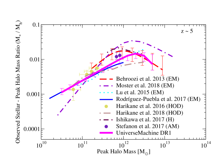
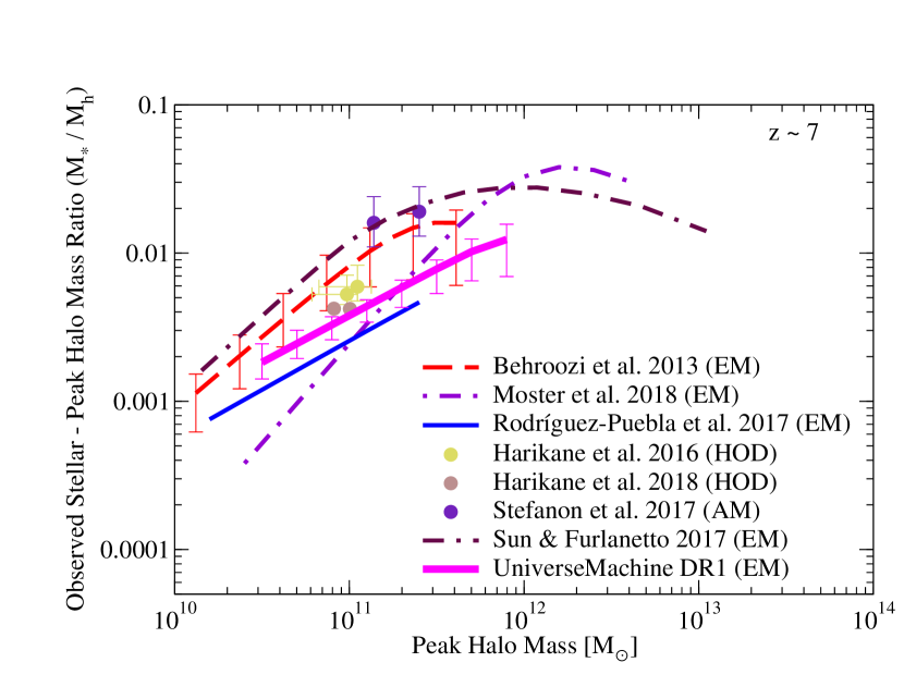
Figure 36: Left: Median stellar mass — halo mass relations for our best-fitting model compared to previous results at $z\sim 5$ and $z\sim 7$. Results compared include those from our previous work (Behroozi et al., 2013e), from empirical modeling (EM; Lu et al., 2015b; Sun & Furlanetto, 2016; Rodríguez-Puebla et al., 2017; Moster et al., 2018), from abundance matching (AM; Stefanon et al., 2017), and from Halo Occupation Distribution modeling (HOD; Harikane et al., 2016, 2018; Ishikawa et al., 2017).

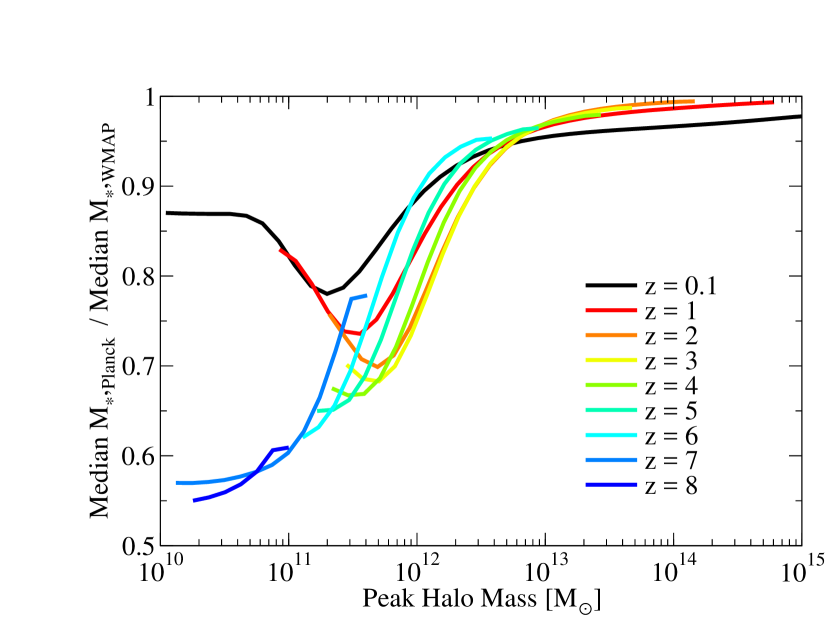
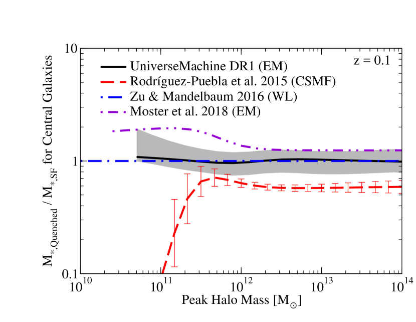
Figure 37: Change in median stellar mass–halo mass relation between WMAP and Planck cosmologies for the SMHM relation in Behroozi et al. (2013e).

Figure 38: Ratio of median stellar mass — halo mass relations for quenched and star-forming central galaxies for our best-fitting model compared to previous results at $z=0.1$. Results compared include those from Conditional Stellar Mass Function modeling (CSMF; Rodríguez-Puebla et al., 2015), from lensing (WL; Zu & Mandelbaum, 2016), and from empirical modeling (EM; Moster et al., 2018). The grey shaded region shows the $16^{\mathrm{th}}-84^{\mathrm{th}}$ percentile range for statistical errors plus an additional 0.1 dex of systematic error in the recovery of stellar mass for star-forming vs. quiescent galaxies (Appendix C.2).

5.8 Orphan Galaxies

Orphans are very strongly preferred in our posterior distribution, with satellite fractions roughly $25\%$ larger than would be expected from the N–body simulation alone. As detailed in Appendix B, this arises because of tension between the need for a large satellite fraction at a given stellar mass (to match the observed autocorrelation for all galaxies) and the need for low satellite star formation rates (to match differences between quenched and star-forming correlation functions). This tension is not helped by the evolution of the stellar mass–halo mass (SMHM) relation to lower efficiencies at $z=1$ compared to $z=0$, as then satellites have even less stellar mass at infall compared to a non-evolving SMHM relation. Many potential resolutions are not self-consistent; e.g., using a stellar mass proxy that gives additional stellar mass to satellites (as in Reddick et al., 2013). Campbell et al. (2018) suggests that it may be possible to resolve this tension self-consistently through other means, including by allowing satellite galaxies to grow after accretion and to have stellar masses that correlate with halo assembly history. Yet, although our model allows (and includes) both these alternative solutions, orphans are still strongly preferred; Moster et al. (2018) reach a similar conclusion.

Observational data could constrain a more complex orphan model than examined here. In our fiducial model, satellites are retained until they fall below a certain $\frac{v_{\mathrm{max}}}{v_{\mathrm{Mpeak}}}$ ratio (i.e., $T_{\mathrm{merge}}$). That said, the most realistic choice of which satellites to retain could also depend on the orbit, the time since infall, and the simulation’s resolution. Additional data, such as the radial profiles of quenched and star-forming galaxies around groups and clusters (e.g., Wetzel et al., 2012), could then provide observational constraints for these more complex orphan models.

5.9 Comparison to Previous Results

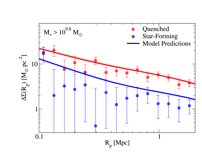
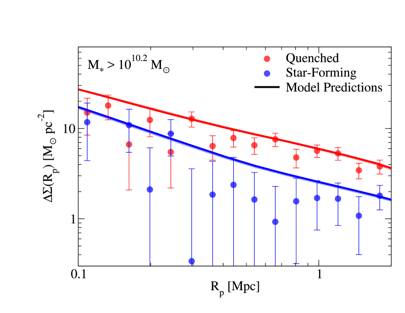
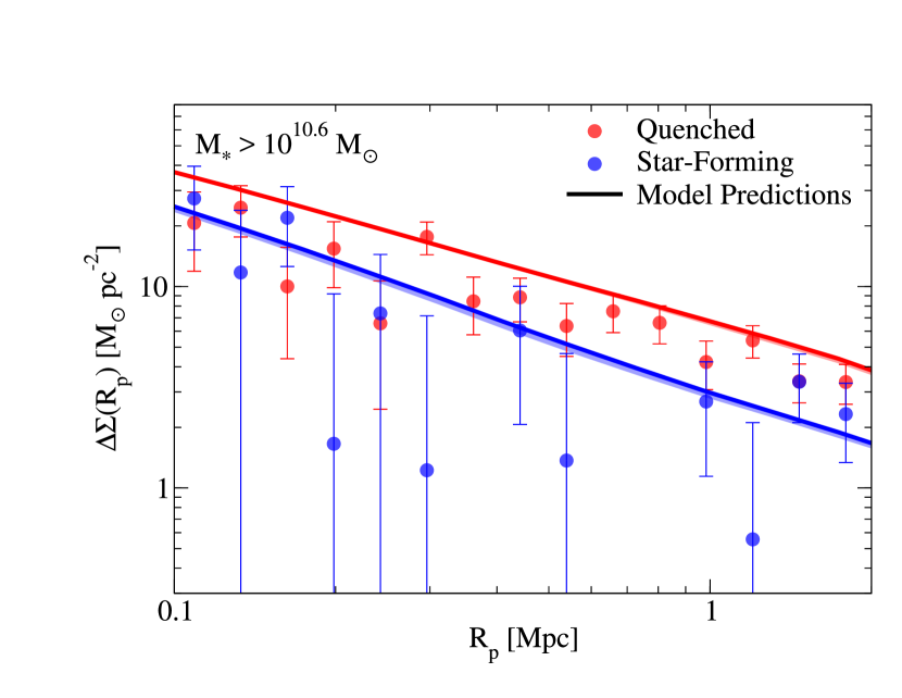
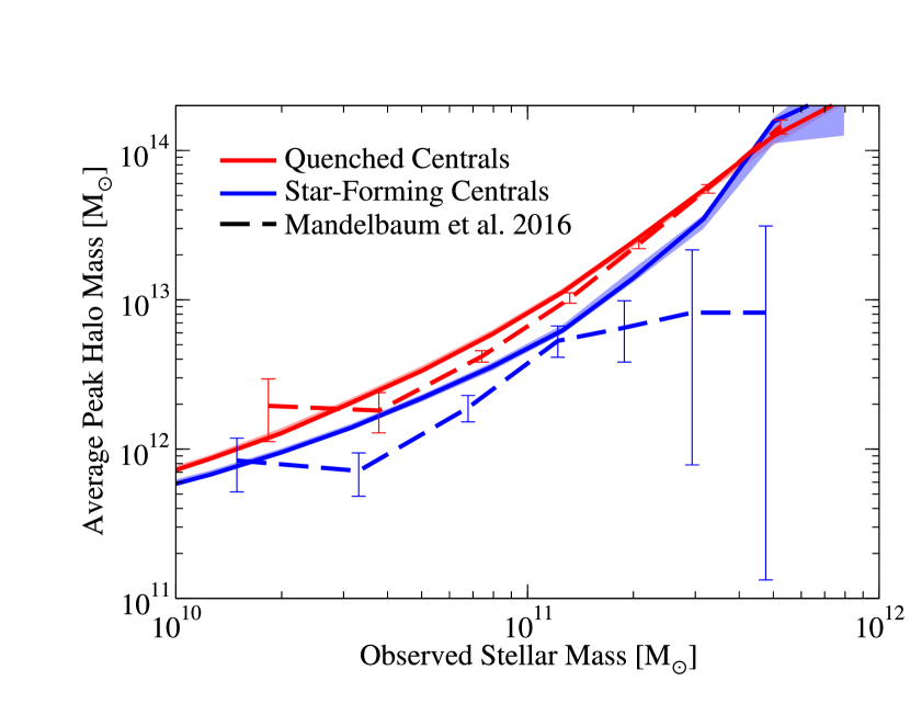
Figure 39: Top and bottom-left panels: Weak lensing excess surface densities ($\Delta\Sigma$) from the best-fitting model at $z=0.1$ compared to observations (Watson et al., 2015) for three $M_{*}$ threshold samples. All distances and areas are in comoving units. Bottom-right panel: Comparison of the mean halo mass as a function of stellar mass for star-forming and quenched central galaxies to the results in Mandelbaum et al. (2016). Notes: consistent with the findings in Leauthaud et al. (2017) that lensing and correlation function measurements are difficult to reconcile, our predicted excess surface densities are $10-30$% higher than the observations.

We compare the median stellar mass – halo mass ratios from the model to past results at $z=0.1$ (Fig. 35), $z=1-3$ (Fig. 35), and $z=5-7$ (Fig. 36). All results have been converted to use the same halo mass definition ($M_{\mathrm{vir}}$; Bryan & Norman 1998). Abundance matching results have been further converted to our adopted Planck cosmology (§2.1); as converting the cosmologies of other techniques requires re-running the original analysis, we have left those as-is. Planck-consistent cosmologies have more haloes at a given mass compared to WMAP, especially at higher redshifts (Rodríguez-Puebla et al., 2016b). The corresponding effect on the SMHM relation depends on $\frac{dM_{\ast}}{dM_{h}}$, with the result that haloes with $M_{h}<10^{12}\;\mathrm{M}_{\odot}$ are more affected than haloes with $M_{h}>10^{12}\;\mathrm{M}_{\odot}$ (Fig. 38).

The comparison agrees extremely well across all redshifts, halo masses, and techniques, with the exception of $M_{h}>10^{13}\;\mathrm{M}_{\odot}$ at $z<1$. As discussed in Appendix C.2, this is due to revised photometry and fitting of massive galaxies in the SDSS, as well as deeper imaging of $z=0-1$ massive galaxies in ULTRAVISTA. Using the revised stellar mass functions resolves past discrepancies between cluster-based SMHM relations and those derived from empirical models (Lin & Mohr, 2004; Hansen et al., 2009; Kravtsov et al., 2018). The remaining difference between our results and Kravtsov et al. (2018) is due to the latter counting all intracluster light as part of the galaxy.

For low-mass haloes ($M_{h}<10^{11}\;\mathrm{M}_{\odot}$), the best-fitting model has a weaker upturn in the SMHM ratio than found by Behroozi et al. (2013e); this is because Behroozi et al. (2013e) assumed a strong surface-brightness incompleteness correction for faint galaxies that is no longer observationally supported (Williams et al., 2016). This will make it easier to reconcile observed galaxy counts with the HI mass function and observed HI gas fractions in faint galaxies (Popping et al., 2015).

The SMHM relation for star-forming vs. quiescent galaxies depends on the correlation between galaxy and halo assembly (§4.2) and the evolution of the SMHM relation (see also Moster et al., 2018). As shown in Fig. 38, there remain significant differences across studies (see also Wechsler & Tinker, 2018). Our model is flexible in terms of both the SMHM relation evolution and the galaxy–halo assembly correlation, and suggests that the stellar mass–halo mass relation at fixed halo mass is similar for star-forming and quiescent central galaxies, matching the conclusion in Zu & Mandelbaum (2016). The results of Moster et al. (2018) and Rodríguez-Puebla et al. (2015) give opposite conclusions of higher and lower (respectively) median stellar masses for quiescent compared to star-forming galaxies, despite using the same underlying data (correlation functions in the SDSS) to constrain their models. In part, these divergent conclusions arise because correlation functions and weak lensing measurements are both very sensitive to satellite clustering; hence, small changes to the satellite halo occupation can lead to large changes in the inferred occupation for central galaxies. Applying a cut to first remove satellites before measuring clustering, environment, or lensing (as in both this study and Zu & Mandelbaum 2016) is hence necessary to robustly determine SMHM differences for star-forming and quiescent central galaxies. As noted in Zu & Mandelbaum (2016) and Moster et al. (2018), having an equivalent median stellar mass at fixed halo mass does not imply that the median halo mass at fixed stellar mass will be equal for star-forming and quiescent galaxies. Because the ratio of star-forming to quiescent galaxies drops rapidly with increasing halo mass, it is much more likely in this case that a given massive star-forming galaxy will be hosted by a lower-mass halo than a massive quiescent galaxy.

We show direct comparisons with lensing ($\Delta\Sigma$) measurements from Watson et al. (2015) in Fig. 39. While the trends are similar, $\Delta\Sigma$ is overestimated by $10-30\%$ for both quenched and star-forming galaxies in the best-fitting model. Leauthaud et al. (2017) also finds that matching galaxy autocorrelation functions results in mock catalogues that overpredict $\Delta\Sigma$ measurements by $20-40\%$. We refer readers to Leauthaud et al. (2017) for further discussion of this tension, while noting that correlation functions and weak lensing measurements are affected differently by the satellite occupation distribution adopted. Fig. 39 also shows a comparison with mean halo mass as a function of stellar mass for central galaxies. Mandelbaum et al. (2016) use stellar masses from the NYU-VAGC (Blanton et al., 2005); we have corrected these to better correspond to the Brinchmann et al. (2004) stellar masses underlying our correlation function measurements using the median offsets between star-forming and quenched galaxies (Fig. 42). We do not attempt to correct the Mandelbaum et al. (2016) results for photometry offsets (Bernardi et al., 2013) as this is less straightforward. The qualitative effects would be both to increase galaxy masses (for $M_{\ast}>10^{11}\;\mathrm{M}_{\odot}$) and to increase inferred host halo masses (via decreasing the scatter in halo mass at fixed galaxy mass; Kravtsov et al. 2018).

In parallel with empirical models, hydrodynamical simulations and semi-analytic models have shown increased success in matching multiple observations (e.g., Schaye et al., 2015; Somerville & Davé, 2015; Henriques et al., 2015; Dubois et al., 2016; Dolag et al., 2016; Croton et al., 2016; Springel et al., 2018). A proper comparison with these results is beyond the scope of this paper; it is hence deferred to future work.

Additional comparisons between figures in this paper and in Behroozi et al. (2013e) are available online.

5.10 Evolution in the Stellar Mass – Halo Mass Relation at z>4

There have been contradictory claims regarding the $z>4$ evolution of the stellar mass–halo mass relation. Many recent studies, including this one, find either significant evolution (Behroozi et al., 2013e; Behroozi & Silk, 2015; Finkelstein et al., 2015b; Harikane et al., 2016, 2018; Sun & Furlanetto, 2016) or modest evolution (Moster et al., 2018). Stefanon et al. (2017) claims to find no evolution, but as is evident from Fig. 36, their findings in fact suggest even stronger evolution than our current results due to the slope of the SMHM relation. In contrast, Rodríguez-Puebla et al. (2017) find very little evolution at $z>4$. This may be in part due to the fact that their assumed scatter in observed vs. true stellar mass grows as $0.1+0.05z$ with no upper bound, so that scatter is $0.5$ dex at $z=8$ and $0.6$ dex at $z=10$, well beyond the $0.3$ dex limit assumed here. In addition, it may be due to the use of UV–SM relations at high redshifts that could underestimate true stellar masses (Appendix D). Despite this, the relative uncertainty in stellar mass estimates at $z>4$ remains large, as shown in Fig. 6 of Moster et al. (2018). Adding to the uncertainty, a non-evolving star formation efficiency (defined as $SFR/\dot{M_{h}}$) can plausibly fit UV luminosity functions from $z=10$ to $z=0$ (Mason et al., 2015; Harikane et al., 2018; Tacchella et al., 2018). As discussed in Behroozi et al. (2013c), this is equivalent to a non-evolving SMHM ratio, and so the Harikane et al. (2018) star formation efficiency model is in tension with the evolving SMHM ratio found in the same paper via clustering analyses. While the match to UV luminosity functions is degenerate with the assumed dust evolution, it is clear that a consistent picture of stellar masses, star formation rates, and dust has yet to emerge at $z>4$. NIRCam and NIRSpec on the James Webb Space Telescope will hence be instrumental in settling this debate (see Kalirai, 2018, for a review).

5.11 Addressing Assumptions and Uncertainties with Additional Data and Modeling

The empirical model herein has broad classes of assumptions relating to the average connection between galaxy SFR and halo mass, the correlation between individual halo and galaxy growth, and the relevance of dark matter simulations for modeling observed galaxies. We address each of these in turn.

External validation of predictions including the stellar mass—halo mass relation (§39) suggests that the model framework is flexible enough to capture how stellar mass and SFR depend on halo mass and redshift. Additional observations will be helpful especially for $z>4$ galaxies (see §5.10 and Appendix D); the model would also benefit by including more constraints on SFRs in massive clusters at $z\sim 1-2$ (see Fig. 14, left panel). Nonetheless, the primary sources of uncertainty for most galaxies are systematic ones–e.g., the conversion between luminosity and physical stellar masses and star formation rates (see §4.10 and Appendices C, D, and G). Addressing these uncertainties with more observations may be difficult due to their dependence on rare stellar populations (e.g., Conroy et al., 2009) and/or uncertain dust geometry distributions (e.g., Narayanan et al., 2018). Forward modeling directly (and only) to luminosities and colours may help, approaching the method in Taghizadeh-Popp et al. (2015). For massive galaxies, there are additional systematics with measuring luminosity profiles at different redshifts (Appendix C.2). These may be improved with surveys that are both wide enough to find many massive galaxies and deep enough to accurately measure their profiles, such as the Hyper Suprime-Cam Subaru Strategic Program survey (HSC-SSP; Aihara et al. 2018).

Empirically connecting individual galaxy and halo growth is a new field, so the observables that best constrain this connection are not yet known. Appendix A discusses several observables that rule out alternative models. Clustering gives powerful constraints on satellite behaviour, so it will be important to continue extending the redshift and mass range of clustering measurements. Despite the observational difficulty, clustering for quiescent galaxies is especially important, as the largest constraining power comes from the contrast between quenched and star-forming galaxy clustering. For isolated central galaxies (i.e., those that have never crossed the virial radius of a larger halo), the importance of the host halo’s assembly history remains debated (Tinker et al., 2017). Connecting observed splashback radii (e.g., as claimed in More et al., 2016) with dark matter accretion rates is a promising path forward for such galaxies, and is planned for future work.

With dark matter simulations, the most critical issues remain subhalo finding (Onions et al., 2012; Behroozi et al., 2015b), satellite disruption (see §5.8 and Appendix B) and the effects of baryons (see, e.g., Nadler et al., 2018; Chua et al., 2017, for recent work). Central halo finding is a more minor issue, especially when (as in this paper) $v_{\mathrm{max}}$ is used as the mass proxy (Knebe et al., 2011, 2013). Subhalo finding is more than a definitional issue, as different halo finders introduce different orbit dependencies in recovered halo properties (Behroozi et al., 2015b); temporal halo finders (including HBT/HBT+; Han et al. 2012; Han et al. 2018) are most immune to this effect. As noted in §5.8 observed satellite properties in group catalogues at different redshifts may represent a promising way to calibrate empirical orphan models; this to some extent will include the effect of baryons. Remaining effects of baryons on halo potential wells (e.g., making them less triaxial; Abadi et al. 2010) are more difficult to observe, and may require higher-order statistics such as three-point functions to capture.

5.12 Future Directions in Empirical Modeling

With empirical modeling, physical constraints from different observables can be combined even when the best underlying parameter space is not known. The same general framework may be applied to many other problems, even outside of galaxy formation. Whereas this paper constrained galaxy SFR as a function of relevant parameters (halo $v_{\mathrm{max}}$, accretion rate, and redshift), one may use the same technique to constrain how any observable $X$ depends on arbitrary parameters $Y_{1},\ldots,Y_{n}$. As of this writing, there are ongoing empirical efforts to constrain how galaxy size, morphology, metallicity, gas content, black hole mass, gamma-ray burst rate, supernova rate, and dust relate to underlying properties of the host dark matter halo, its assembly history, and the resulting galaxy’s assembly history. These applications promise a wealth of new physical insight about our Universe in the years to come (Behroozi et al., 2019).

6 Conclusions

Our model (§3) flexibly parametrizes the correlation between galaxy assembly and halo assembly, and is able to self-consistently match a broad array of observational data (§4, 4.5, 39). The following results are robust to the modeling uncertainties.

For the stellar mass–halo mass relation:

• Consistent with past results, haloes near $10^{12}\;\mathrm{M}_{\odot}$ are most efficient (20-40%) at turning gas into stars at all redshifts (§4.2).

• While the stellar mass–halo mass relation does not evolve significantly from $z=0$ to $z\sim 5$, significant evolution does occur at higher redshifts (§4.2) with present data (§5.10).

• At $z=0$, massive quiescent galaxies reside in higher-mass haloes than massive star-forming galaxies (§39). Due to scatter in the stellar mass–halo mass relationship, it is also true that quiescent galaxies are more massive at fixed halo mass than star-forming galaxies for $M_{h}>10^{13}\;\mathrm{M}_{\odot}$ at $z=0$ (§4.2).

For quenching and galaxy–halo assembly correlations:

• Quenching is highly correlated with halo mass, where a difference of $\lesssim 1.5$ dex in host halo mass separates largely star-forming populations from largely quenched ones (§4.3).

• At $z<1$, satellite quenching becomes more important, so quenching happens over a broader range of halo masses (§4.3).

• The correlation between galaxy and halo assembly is strong, but not perfect (correlation coefficient $\sim 0.5-0.6$; §4.6). High-redshift observations of correlation functions and weak lensing will test the galaxy–halo assembly correlation strength at $z>1$; we also make predictions for these measurements (§4.9).

• Average quenched fractions robustly decrease with increasing redshift at fixed halo mass (§4.3), suggesting that cooling times are not solely responsible for quenching (§5.2).

• Except for cluster cores, where satellites quench very quickly, the fraction of quenched satellites minus the fraction of quenched centrals never exceeds $35\%$ at fixed stellar mass (§4.7).

• Satellites quench faster the more massive they are (§4.7).

In addition:

• Most galaxy mass formed in-situ for $M_{h}\leq 10^{12}\;\mathrm{M}_{\odot}$ haloes (§4.8). Low-mass galaxies ($M_{\ast}<10^{9}\;\mathrm{M}_{\odot}$) are predicted to have significant ($\gtrsim 1$ dex) scatter in their intrahalo light (§4.8).

• Planck cosmologies have more low-mass haloes at high redshifts, lowering the inferred stellar mass–halo mass relation by up to 0.3 dex compared to WMAP cosmologies (§39).

The following results, while robust given the observational constraints, depend on the modeling assumptions:

• Satellite galaxies have very broad ($3-5$ Gyr) quenching delay-time distributions after infall (§4.7).

• If the correlation between galaxy and halo assembly history is also strong for central galaxies that have not interacted with larger haloes, then past rejuvenation (quenching followed by renewed star formation) is common for $M_{\ast}\sim 10^{11}\;\mathrm{M}_{\odot}$ galaxies and $M_{h}\sim 10^{12.5}\;\mathrm{M}_{\odot}$ haloes at $z=0$ (§4.6).

• Quenched galaxies at $z=0$ have significantly different average star formation histories than star-forming ones out to $\sim 3$ Gyr, which can aid in tracing average galaxy populations through cosmic time (§4.5). However, individual galaxies have significant scatter in star formation histories, making the comparison across redshifts less well constrained (§4.5).

All code, mock catalogues, and data products (§4.11) are available online.

Appendix A Alternate Parameterizations of Halo Assembly History

The following alternate conditional abundance matching (CAM) parameters were tried and rejected, as detailed below.

A.1 Classical Age-Matching ($z_{\mathrm{starve}}$)

CAM using the $z_{\mathrm{starve}}$ parameter is known to reproduce galaxy clustering, weak lensing, and radial quenching profiles around groups and clusters (Hearin & Watson, 2013; Hearin et al., 2015; Watson et al., 2015). While $z_{\mathrm{starve}}$ is a complicated function, for most haloes it is equivalent to rank ordering on $\frac{c_{\mathrm{acc}}}{a_{\mathrm{acc}}}$, where $c_{\mathrm{acc}}$, and $a_{\mathrm{acc}}$ are the concentration and scale factor (respectively) at accretion (for satellites) or at the present day (for centrals).

There are several minor issues with $z_{\mathrm{starve}}$ that, while all fixable, would have made the parameter even less transparently physical than it already is. These include:

1. Special treatment for satellites (in the form of $c_{\mathrm{acc}}$ and $a_{\mathrm{acc}}$) leading to unphysical discontinuities for backsplash haloes (i.e., haloes that enter and leave the virial radius of a larger halo).

2. No orbit-dependent SFRs for satellites.

3. Increased concentrations during the early stages of major mergers would result in decreased SFRs, instead of the expected boost prior to the merger. Afterwards, decreased concentrations would result in increased SFRs, instead of the expected post-starburst phase.

A.2 Mass Accretion History

This has been used by many other studies (Becker, 2015; Rodríguez-Puebla et al., 2016a; Cohn, 2017; Moster et al., 2018). Satellites are the clearest issue: while the fraction of satellite haloes increases towards lower halo masses (Behroozi et al., 2013b; Rodríguez-Puebla et al., 2016b), the fraction of quenched galaxies decreases (Salim et al., 2007; Geha et al., 2012). Hence, many satellite galaxies are still forming stars even though their host (sub)haloes are losing mass. While it’s possible to rank-order satellites on their mass-loss rate, measuring subhalo masses is notoriously difficult (Onions et al., 2012), and is thus extremely sensitive to the halo finder. Alternate solutions include measuring the time since $M_{\mathrm{peak}}$ was reached (Moster et al., 2018), although this erases any differences between different orbits after infall.

With mass accretion rates, an open question is which mass definition best correlates with galaxy assembly (e.g., a specified spherical overdensity, the mass within the splashback region, etc.). A related issue is that pseudo-evolution (i.e., “mass accretion” due to a changing overdensity definition) dominates the mass accretion rate at $z=0$ (Diemer et al., 2013), so that for most central haloes, the mass accretion rate is really measuring the halo concentration (i.e., it becomes equivalent to using $z_{\mathrm{starve}}$). As shown in Wetzel & Nagai (2015), this may not be a problem after all, as this “mass accretion rate” is a reasonable estimate of the gas that actually makes it to the halo center—also suggesting that $z_{\mathrm{starve}}$ works in part due to its correlation with mass assembly.

A more serious issue is that current studies correlating halo mass growth with galaxy SFRs do not distinguish between smooth mass accretion and mergers. Behroozi et al. (2015a) showed that field galaxies in haloes undergoing major mergers (observationally identifiable as close galaxy pairs) have nearly identical quenched fractions as more typical field galaxies; mock observations applied to mock catalogues with mass accretion – SFR correlations were significantly discrepant from the real observations. This may be fixable by correlating only smooth mass accretion rates with galaxy SFRs (i.e., discounting the effects of major and minor mergers), but doing so would require higher resolution simulations than are currently practical to use.

A.3 Tidal Forces

Tidal forces are robustly calculable for satellites and would also introduce clearly orbit-dependent effects in their star formation histories. Yet, connecting high tidal forces with quenching would require that voids (i.e., regions with low tidal forces) should primarily contain star-forming galaxies, which has less observational support. We tested this in the Sloan Digital Sky Survey (SDSS), selecting extremely isolated $L^{*}$ galaxies (i.e., a stellar mass-complete sample with $10^{10}<M_{\ast}/\;\mathrm{M}_{\odot}<10^{10.5}$; no larger neighbour within 4 Mpc projected or 2000 km/s redshift distance) and comparing them to “normal” $L^{*}$ field galaxies (i.e., same stellar mass cut; no larger neighbour within 500 kpc projected or 1000 km/s redshift distance). Using mock catalogues from Behroozi et al. (2015a), we verified that the majority of extremely isolated galaxies had tidal forces in the 15^th percentile or lower, and that 90% had tidal forces in the 50^th percentile or lower, as compared to the normal field galaxies. However, in the SDSS, quenched fractions were indistinguishable between the extremely isolated galaxies and the normal field galaxies (see also Croton & Farrar 2008).

Separately, Lee et al. (2017) has examined central halo assembly as a function of environment. While many halo properties (concentration, spin, mass accretion history) are strongly affected in dense environments with large tidal forces, halo properties in extremely underdense environments (with very low tidal forces) are almost indistinguishable from halo properties in median-density environments. Hence, weak tidal forces do not appear to correlate with internal halo (and presumably galaxy) properties to the same extent as strong ones do.

A.4 Simpler $v_{\mathrm{max}}$ Prescriptions

We considered many simpler $v_{\mathrm{max}}$ prescriptions, including $\frac{v_{\mathrm{max}}(z_{\mathrm{now}})}{v_{\mathrm{max}}(z_{\mathrm{dyn}})}$. However, this prescription required continuing mass loss for quenching. Hence, reinfalling satellites were not quenched at high enough rates, regardless of the number of orbits they had made. This resulted in not enough separation between correlation functions for quenched and star-forming galaxies. We also considered $\frac{v_{\mathrm{max}}(z_{\mathrm{now}})}{v_{\mathrm{Mpeak}}}$ (and its close relative $\frac{v_{\mathrm{max}}(z_{\mathrm{now}})}{v_{\mathrm{peak}}}$). This dramatically improved clustering, but then caused issues for central galaxies: most centrals have $v_{\mathrm{max}}(z_{\mathrm{now}})=v_{\mathrm{Mpeak}}$, as they are continuously growing in mass. Similarly, $\frac{v_{\mathrm{max}}(z_{\mathrm{now}})}{v_{\mathrm{peak}}}$ was strongly peaked—so that small errors in recovering $v_{\mathrm{max}}$ (e.g., from the halo finder) would result in huge variations in halo rank order.

Appendix B Orphan Galaxies

B.1 The Need for Orphans

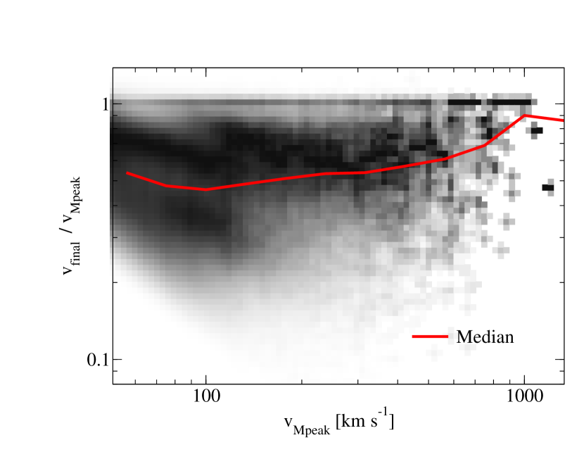
Figure 40: Conditional distribution of the ratio between the final detectable $v_{\mathrm{max}}$ and $v_{\mathrm{Mpeak}}$ for subhaloes that disappeared between $z=1$ and $z=0$ in the Bolshoi-Planck simulation. A quarter of massive subhaloes ($v_{\mathrm{Mpeak}}>200$ km s^-1) had more than 70% of their initial $v_{\mathrm{max}}$ at the time they disappeared. The nominal completeness limit for Bolshoi-Planck is $v_{\mathrm{max}}=$50 km s^-1.

“Orphan” galaxies (i.e., galaxies whose host subhaloes are no longer detectable by a halo finder) have not been required by most previous empirical models (Reddick et al., 2013) to match clustering constraints. This is because satellite fractions can be boosted to the required level either by increasing the stellar mass at fixed satellite mass (or $v_{\mathrm{max}}$) or by increasing the number of satellites at a given mass—i.e., by adding orphans. Hence, if orphans are not included, one is forced to conclude that satellite haloes have larger stellar masses than central haloes at fixed $M_{\mathrm{peak}}$ at $z=0$ (Rodríguez-Puebla et al., 2012; Reddick et al., 2013; Watson & Conroy, 2013).

However, we contrast this conclusion with the known evolution of satellite galaxies. Satellites are more quenched than field galaxies (e.g., Wetzel et al., 2012), and hence formed their stars earlier (at $z=1-2$) than central galaxies of the same $M_{\mathrm{peak}}$. At $z=1-2$, the stellar mass–halo mass ratio was likely lower (and certainly no higher) than the ratio at $z=0$ (Moster et al., 2013; Behroozi et al., 2013e). Hence, satellites started out with lower stellar masses, could not grow as efficiently (due to being more quenched), and lost more stellar mass from passive stellar evolution (due to older average stellar ages) compared to central galaxies of the same $M_{\mathrm{peak}}$. We thus are forced to conclude that adding orphans is a more self-consistent way to reproduce observed galaxy clustering constraints (see also Campbell et al. 2018).

A separate reason to include orphans is shown in Fig. 40. The extent to which satellites survive is dependent on the simulation (Klypin et al., 1999), the halo finder (Onions et al., 2012), and the baryonic physics included (Zolotov et al., 2012). The point at which haloes disappear in our simulation (Bolshoi-Planck) may have no relationship with when galaxies tidally disrupt. For example, considering massive haloes only ($v_{\mathrm{Mpeak}}>200$ km s^-1), a quarter of those that disappeared had $v_{\mathrm{max}}>0.7v_{\mathrm{Mpeak}}$—i.e., $>16\%$ of their infall mass remaining (Jiang & van den Bosch, 2016). While it is plausible that a satellite galaxy could tidally disrupt with this much stripping, it’s also plausible that satellite galaxies persist for much longer. Hence, not including orphans imposes a strong, arbitrary prior on satellite evolution, yielding artificially tight constraints on quenching timescales and star formation histories.

B.2 Tracking Method

When a satellite halo becomes undetectable, we identify the parent halo (i.e., a larger halo containing the satellite within its virial radius) to which it is most bound, and follow the satellite’s evolution according to a softened gravity law:

$$\dot{\mathbf{v}}=-\frac{GM(<r)}{(r+0.1R_{\mathrm{vir}})^{2}}\hat{\mathbf{r}},$$ (32)

where $\mathbf{v}$ is the satellite’s peculiar velocity, $R_{\mathrm{vir}}$ is the parent’s virial radius, and $M(<r)$ is the mass of the parent halo enclosed within the satellite–parent distance ($r$)—assumed to follow a Navarro et al. (1997) profile:

$$M(<r)=4\pi\rho_{0}r_{s}^{3}\left[\ln\left(1+\frac{r}{r_{s}}\right)-\frac{r}{r+r_{s}}\right].$$ (33)

The force law is softened as hard collisions are impossible with spatially-extended satellites; as with past approaches, we use leapfrog integration with 10 sub-timesteps per simulation timestep (Behroozi et al., 2013a; Behroozi et al., 2013d). Each sub-timestep is then on the order of $1\%$ of a dynamical time.

To track the satellite’s mass loss, we adopt the orbit-averaged mass-loss prescription of Jiang & van den Bosch (2016), with a small modification. Both synthetic (Knebe et al., 2011) and cosmological (Fig. 1 of Behroozi et al., 2014a) tests show that subhaloes lose almost no mass on infall, but instead lose mass (and $v_{\mathrm{max}}$) steadily after passing pericenter. We hence take:

$$\dot{m}_{\mathrm{infalling}} = 0$$ (34)

$$\dot{m}_{\mathrm{outgoing}} = -1.18\frac{m}{t_{\mathrm{dyn}}}\left(\frac{m}{M}\right)^{0.07},$$ (35)

where $m$ is the satellite’s mass, $M$ is the parent halo’s mass, $\rho_{\mathrm{vir}}$ is the virial overdensity from Bryan & Norman (1998), and we have adjusted the leading constant for $\dot{m}_{\mathrm{outgoing}}$ from Jiang & van den Bosch (2016) for scatter, our different definition of $t_{\mathrm{dyn}}$ ($(\frac{4}{3}\pi G\rho_{\mathrm{vir}})^{-\frac{1}{2}}$), and our assumption that all the mass loss occurs over half the orbit.

To determine $v_{\mathrm{max}}$, we recast the fitting formula from Jiang & van den Bosch (2016):

$$\frac{d\log v_{\mathrm{max}}}{d\log m}=0.3-0.4\frac{m}{m+m_{i}},$$ (36)

where $m_{i}$ is the satellite’s mass at first infall.

As discussed in §3.3, satellites are no longer tracked once the ratio $\frac{v_{\mathrm{max}}}{v_{\mathrm{Mpeak}}}$ falls below $T_{\mathrm{merge}}$. We also remove a very small fraction ($<1\%$) of satellites that are highly unbound (kinetic $>2\times$ potential energy), as those would otherwise travel unphysical distances and require much greater communications overhead between processors.

Appendix C Observational Data Compilation, Calibrations, Exclusions, and Uncertainties

C.1 Overview

Table 4: Adopted Modeling Assumptions for Stellar Mass Functions

Assumption	Publication
Initial Mass Function	Chabrier (2003)
Stellar Population Synthesis	Bruzual & Charlot (2003)
Dust	Calzetti et al. (2000)

Here, we discuss the stellar mass functions (SMFs), star formation rates (SFRs), quenched fractions(QFs), correlation functions (CFs), and higher-order galaxy statistics used as model constraints. Modeling assumptions are inherent to galaxy stellar masses and SFRs (see Conroy 2013, Madau & Dickinson 2014, and Mobasher et al. 2015 for reviews). In this paper, we standardize assumptions for SMFs (Table 4) because discontinuities in modeling assumptions manifest as unphysical discontinuities in galaxy evolution. Notably, assumptions in Table 4 were the only ones for which data were consistently available across the entire redshift range considered.

For SFRs, standardizing on the IMF appears important, but using the same SPS and dust model does not guarantee self-consistency between SMFs and SFRs (Madau & Dickinson, 2014; Leja et al., 2015; Tomczak et al., 2016, and references therein). Yet, the growth of SMFs appears reasonable within the current range of assumptions used to calculate SFRs and SSFRs (Moster et al., 2013; Behroozi et al., 2013e). Hence, as in Behroozi et al. (2013e), we conducted a review of cosmic and specific SFR constraints published since 2007 (see also Madau & Dickinson, 2014; Speagle et al., 2014). Earlier constraints were excluded due to incorrect dust assumptions strongly affecting derived $z>2$ SFRs (see discussion in Behroozi et al. 2013e).

We measure CFs and higher-order statistics directly from the Sloan Digital Sky Survey (SDSS) instead of using past results. This ensures that observed data and models are treated in exactly the same way, that corrections for stellar mass modeling assumptions can be applied self-consistently, and that covariance matrices can be computed using the same code.

All data in this compilation are available in a convenient standard format online.

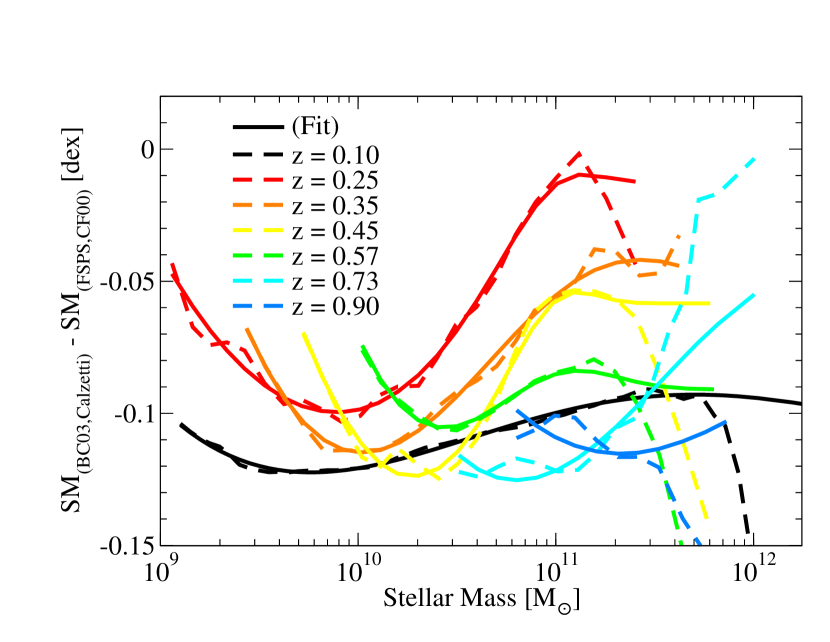
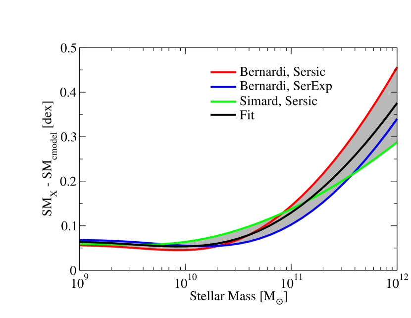
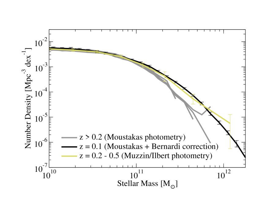
Figure 41: Top panel: stellar mass differences between model assumptions in Moustakas et al. (2013) (i.e., the FSPS SPS model and Calzetti dust law) and our adopted assumptions (Table 4). Middle panel: range of corrections to SDSS stellar masses using cmodel photometry at $z\sim 0.1$. Black line corresponds to our adopted correction; the grey shaded region corresponds to the increase in the error budget from photometry uncertainties. Bottom panel: effect of photometry choices on SMFs for massive galaxies at $z<1$.

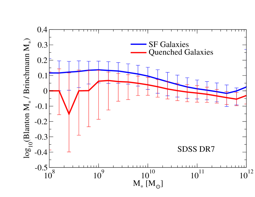
Figure 42: Median offsets between stellar masses in the Brinchmann et al. (2004) and Blanton et al. (2005) catalogues, split for star-forming and quenched galaxies. Error bars correspond to 68% of the scatter between the two catalogues.

C.2 Stellar Mass Functions

Table 5: Observational Constraints on the Stellar Mass Function

Publication	Redshifts	colours	Area (deg2)	Notes
Baldry et al. (2012)	0.002-0.06	ugriz	143	N
Moustakas et al. (2013)	0.05 - 1	UV-MIR	9	SDP
Tomczak et al. (2014)	0.2 - 3	UV-Ks	0.08	N
Ilbert et al. (2013)	0.2 - 4	UV-Ks	1.5	NM
Muzzin et al. (2013)	0.2 - 4	UV-Ks	1.5	INM
Song et al. (2016)	4 - 8	UV-MIR	0.08	NUF

Notes. Letters correspond to conversions applied to the published results: I (Initial Mass Function), S (Stellar Population Synthesis model), D (Dust model), P (Photometry), U ($M_{\ast}-$UV relation). The letter “N” indicates that the constraint was not previously used in Behroozi et al. (2013e). The letter “M” indicates that results from Ilbert et al. (2013) and Muzzin et al. (2013) were merged into a single set of constraints to avoid double-counting the same data sources. “F” indicates that the original data were re-fit using different assumptions (see Appendix D). Local results ($z<0.2$) in the Moustakas et al. (2013) mass functions are taken from the SDSS and cover an area of 2505 deg².

Table 5 lists our adopted SMF constraints. All of the SMFs in this study used the model assumptions in Table 4 except for those from PRIMUS (Moustakas et al., 2013), which used FSPS (Conroy et al., 2009) as the SPS model and CF00 (Charlot & Fall, 2000) as the dust model. Alternate PRIMUS mass functions using the assumptions [FSPS, Calzetti] and [BC03, CF00] were available; however, the combination [BC03, Calzetti] was not available. As a compromise, we computed the stellar mass offsets at fixed cumulative number density between the PRIMUS default mass function ([FSPS, CF00]) and the [FSPS, Calzetti] mass function, and used smooth fits to these offsets to shift the masses in the [BC03, CF00] mass function to approximate a [BC03, Calzetti] mass function. On average, the offsets were $-0.05$ to $-0.1$ dex when converting from the CF00 dust model to the Calzetti dust model, as shown in Fig. 41, top panel.

The cmodel magnitudes used for the $z\sim 0.1$ SMF in Moustakas et al. (2013) underestimate galaxies’ true luminosities due to the SDSS DR7 sky-subtraction algorithm and the profile-fitting routines used (Simard et al., 2011; Bernardi et al., 2013; Bernardi et al., 2017, 2016; D’Souza et al., 2015). Kravtsov et al. (2018) argues that using the Moustakas et al. (2013) SMFs overestimates both the impact of AGN feedback and the scatter in the halo mass—stellar mass relation for massive galaxies; the latter effect also reduces clustering for massive galaxies (Bernardi et al., 2016). We compute the stellar mass offset at constant number density between the cmodel SMF and the average of the SMFs for the three fitting methods in Bernardi et al. (2013) (i.e., Simard et al. 2011 Sérsic, Bernardi et al. 2013 Sérsic, and Bernardi et al. 2013 SérExp) and apply this as a correction (Fig. 41, middle panel) to the Moustakas et al. (2013) $z\sim 0.1$ SMF. We also expand the error budget to encompass the minimum and maximum correction among the three methods. The resulting $z\sim 0.1$ SMF is shown in Fig. 41, bottom panel. It is then apparent that the $z>0.2$ SMFs in Moustakas et al. (2013) suffer from similar photometry problems—i.e., it is unphysical for the number density of $M_{\ast}>10^{11.5}\;\mathrm{M}_{\odot}$ galaxies to be non-evolving from $z=1$ to $z=0.2$ but then to double from $z=0.2$ to $z=0.1$ (Fig. 41, bottom panel). By comparison, the SMFs from Ilbert et al. (2013) and Muzzin et al. (2013) are measured from much deeper photometry and appear more consistent with the corrected $z\sim 0.1$ SMF (Fig. 41, bottom panel). Hence, we truncate the $z>0.2$ constraints from Moustakas et al. (2013) to galaxies with $M_{\ast}<10^{11}\;\mathrm{M}_{\odot}$ to avoid inconsistencies in the photometry of massive galaxies.

We do not apply photometry corrections to the Baldry et al. (2012) SMF, as they infer stellar masses from Sérsic magnitudes (see Hill et al. 2011 for a comparison to SDSS cmodel magnitudes). However, the GAMA source data overlaps entirely with the SDSS for bright galaxies over their redshift range ($0<z<0.06$), so we exclude data points from their SMF with $M_{*}>10^{9}\;\mathrm{M}_{\odot}$ (i.e., the lower limit of the Moustakas et al. 2013 $z\sim 0.1$ SMF). In contrast to Behroozi et al. (2013e), we do not apply a surface brightness incompleteness correction, as recent evidence suggests it is not necessary (Williams et al., 2016).

Both the Ilbert et al. (2013) and Muzzin et al. (2013) SMFs are measured from near-identical data sources (i.e., same fields, same filters, very similar depths) with near-identical stellar mass modeling assumptions. Encouragingly, both studies’ measurements are largely within each others’ error bars, but there are occasions (especially $2<z<2.5$) where this is not the case. To avoid double-counting the same data, we merge the two sets of SMFs into a single set by taking the geometric average between the two studies SMFs, after dividing the Muzzin et al. (2013) stellar masses by a factor of 1.07 to convert from their Kroupa (2001) IMF to our adopted Chabrier (2003) IMF. Where necessary, we increase the error budget to accommodate the 68% confidence regions of both studies’ results.

Stellar masses at $z>3.5$ suffer large systematic uncertainties (Stefanon et al., 2015; Stefanon et al., 2017; Rodríguez-Puebla et al., 2017; Moster et al., 2018), with literature estimates of mass functions and UV–SM relations differing by up to 0.5 dex (Duncan et al., 2014; Song et al., 2016). We investigate in Appendix D, finding that uncertainties in star formation history (SFH) priors dominate other sources of error. Combining the SED data in Song et al. (2016) with constraints on SFHs from the redshift evolution of UV luminosity functions (Papovich et al., 2011) and constraints on galaxy dust content (Bouwens et al., 2016b), we derive improved estimates of UV–stellar mass relations as a function of redshift. Briefly, reproducing the UV–stellar mass relations in Song et al. (2016) requires unphysically short star formation histories; more realistic extended histories result in $\sim 0.3$ dex higher median stellar masses at fixed luminosity, even after accounting for nebular emission lines.

Finally, we note that the choice of SPS and dust models results in a bias that is generically different for star-forming and quenched galaxies. For example, Fig. 42 shows differences between the Brinchmann et al. (2004) and Blanton et al. (2005) stellar mass estimates. The offsets between the two are consistently higher for star-forming galaxies compared to quenched ones. As the offsets with true galaxy stellar masses are unknown, caution must be taken when comparing properties for quenched and star-forming galaxies that have a strong dependence on stellar mass (e.g., host halo mass).

C.3 Cosmic and Specific SFRs

Table 6: Observational Constraints on the Cosmic Star Formation Rate

Publication	Redshifts	Type	Area (deg2)	Notes
Robotham & Driver (2011)	0-0.1	UV	833	I
Salim et al. (2007)	0-0.2	UV	741
Gunawardhana et al. (2013)	0-0.35	H$\alpha$	144	IN
Ly et al. (2011a)	0.8	H$\alpha$	0.8	I
Zheng et al. (2007)	0.2-1	UV/IR	0.46
Rujopakarn et al. (2010)	0-1.2	FIR	0.4-9	I
Drake et al. (2015)	0.6-1.5	[OII]	0.63	N
Shim et al. (2009)	0.7-1.9	H$\alpha$	0.03	I
Sobral et al. (2014)	0.4-2.3	H$\alpha$	0.02-1.7	N
Magnelli et al. (2011)	1.3-2.3	IR	0.08	I
Karim et al. (2011)	0.2-3	Radio	2
Santini et al. (2009)	0.3-2.5	IR	0.04	IN
Ly et al. (2011b)	1-3	UV	0.24	I
Kajisawa et al. (2010)	0.5-3.5	UV/IR	0.03	I
Schreiber et al. (2015)	0-4	FIR	1.75	IN
Planck Collab. et al. (2014)	0-4	FIR	2240	IN
Dunne et al. (2009)	0-4	Radio	0.8	I
Cucciati et al. (2012)	0-5	UV	0.6	I
Le Borgne et al. (2009)	0-5	IR-mm	varies	I
van der Burg et al. (2010)	3-5	UV	4	I
Yoshida et al. (2006)	4-5	UV	0.24	I
Finkelstein et al. (2015a)	3.5-8.5	UV	0.084	IN
Kistler et al. (2013)	4-10.5	GRB	varies	IRN

Notes. Letters correspond to conversions applied to the published results: I (Initial Mass Function), R (CSFR normalization for GRBs). The letter “N” indicates that the constraint was not previously used in Behroozi et al. (2013e). The technique of Le Borgne et al. (2009) (parametric derivation of the cosmic SFH from counts of IR-sub mm sources) uses multiple surveys with different areas. Kistler et al. (2013) used GRB detections from the Swift satellite, which has a FOV of $\sim 3000$ deg² (fully coded) and $\sim$10000 deg² (partially coded).

Table 7: Observational Constraints on Average SSFRs

Publication	Redshifts	Type	Area (deg2)	Notes
Salim et al. (2007)	0-0.2	UV	741
Bauer et al. (2013)	0-0.35	H$\alpha$	144	N
Whitaker et al. (2014)	0-2.5	UV/IR	0.25	N
Zwart et al. (2014)	0-3	Radio	1	IN
Karim et al. (2011)	0.2-3	Radio	2
Kajisawa et al. (2010)	0.5-3.5	UV/IR	0.03	I
Schreiber et al. (2015)	0-4	FIR	1.75	IN
Tomczak et al. (2016)	0.5-4	UV/IR	0.08	N
Salmon et al. (2015)	3.5-6.5	SED	0.05	IN
Smit et al. (2014)	6.6-7	SED	0.02	IN
Labbé et al. (2013)	7.5-8.5	UV/IR	0.040	I
McLure et al. (2011)	6-8.7	UV	0.0125	I

Notes. Letters correspond to conversions applied to the published results: I (Initial Mass Function). The letter “N” indicates that the constraint was not previously used in Behroozi et al. (2013e). While Bauer et al. (2013) did not provide average SSFR constraints directly, they released a public catalogue of SSFRs (included in Liske et al., 2015), from which we computed averages. We obtained average SSFRs from Schreiber et al. (2015) by multiplying average SSFRs for star-forming galaxies by $(1-f_{q}$), where $f_{q}$ was the reported quenched fraction. Zwart et al. (2014) assumed a Chabrier (2003) IMF for stellar masses but a Salpeter (1955) IMF for SFRs.

Tables 6 and 7 list our adopted CSFR and SSFR constraints, respectively. As for stellar mass functions, we standardize on the Chabrier (2003) IMF for specific (SSFRs) and cosmic (CSFRs) star formation rates. For SSFRs, we divide stellar masses derived from Kroupa (2001) and Salpeter (1955) IMFs by factors of 1.07 and 1.7, respectively, to convert to a Chabrier (2003) IMF. For both SSFRs and CSFRs, we divide SFRs by factors of 1.06 and 1.58, respectively, for the same conversions (from Salim et al., 2007).

As noted in Appendix C.1, we do not enforce further assumptions in Table 4, as those do not guarantee self-consistency between SMFs and SFRs. For $z<4$ constraints, we excluded studies using fewer than 50 galaxies per redshift bin. We also excluded SSFR studies that did not use mass-selected samples (e.g., main-sequence-only studies), as incorporating dozens of individual studies’ selections would have dramatically increased the complexity of the modeling code. Notably, this requirement excluded using SSFRs from H$\alpha$-selected samples. Studies that did not provide enough details to model their results—including not providing the assumed IMF, the redshift range, or (in the case of SSFRs) a stellar mass range—were also excluded. Notably, the redshift range requirement led to a preference for studies using photometric or spectroscopic redshifts, as opposed to, e.g., dropout selection techniques. Finally, we excluded studies whose results were superseded by a later work.

Emission-line (EL)-derived SFRs (e.g., from H$\alpha$) deserve special consideration. Gunawardhana et al. (2013) argue that spectroscopic surveys allow better estimation of contamination and extinction, but suffer from bivariate selection (i.e., preselecting galaxies by their optical magnitude before determining EL flux) so that they require incompleteness corrections at low EL luminosities. They also demonstrate that H$\alpha$ narrowband surveys at $z<0.1$ have significant scatter ($\sim 1$ dex) due to cosmic variance; Drake et al. (2013) mentions further evidence of significant ($\sim 0.5$ dex) cosmic variance even for $\sim 1$ deg² narrowband surveys to $z=0.4$. Hence, we exclude uncorrected spectroscopic EL and $z<0.5$ narrowband EL measurements from this compilation. We note that some studies using ELs assume constant extinction (e.g. Sobral et al., 2014). As EL extinction correlates with stellar mass (e.g., Hopkins et al., 2001; An et al., 2014), assuming constant extinction will underestimate SFRs for massive galaxies and overestimate them for faint ones. That said, we have tested the net effect on the CSFR from mass-dependent extinction according to An et al. (2014) and found a difference of $\sim 0.1$ dex compared to the constant extinction assumption in Sobral et al. (2014), which is less than other major sources of systematic error at that redshift (see also Gunawardhana et al., 2013). We note that the assumption in Drake et al. (2015) of a constant [OIII]/H$\beta$ ratio is incorrect (Dickey et al., 2016) and significantly underestimates the CSFR; hence, we exclude [OIII]-derived CSFRs from that study.

For $z>4$ constraints, it was no longer possible to require mass-selected samples for SSFRs. However, observed quenched fractions decline from $z=0$ to $z\sim 3-4$ (Muzzin et al., 2013) and theoretical expectations (Jaacks et al., 2012b; Behroozi & Silk, 2015) suggest that the majority of $z>4$ galaxies should be star-forming. However, we excluded SSFR studies that did not account for nebular emission lines, which would otherwise bias stellar masses high by $\sim$0.3 dex (Stark et al., 2013).

At $z>4$, the majority of CSFR constraints are based on UV-derived SFRs. Because of steep reported faint-end slopes in the UVLF (Bouwens et al., 2015), estimating the total CSFR is subject to large uncertainties, and most studies choose to integrate to a specified lower luminosity limit. In this work, we adopt the lower luminosity limit of Finkelstein et al. (2015a) of $M_{UV}=-17$ and convert other UV-based studies to this threshold using their provided Schechter-function fits for the UVLF. Low number statistics at $z\sim 9$ and $z\sim 10$ (Bouwens et al., 2015) pose a special challenge. Oesch et al. (2014) report an exceptionally low CSFR compared to extrapolations of lower-redshift trends, as well as expectations from SSFRs at lower redshifts (Behroozi & Silk, 2015; Finkelstein et al., 2015a). At least in part, this was because Oesch et al. (2014) assumed that luminosity bins with no detected galaxies did not contribute to the CSFR; a more physically reasonable prior (e.g., a Schechter function) substantially revises their estimate for the CSFR (S. Finkelstein et al., in prep.). Because of the resulting bias, we do not use CSFR constraints from UV studies at $z>8$, instead opting to compare to the luminosity functions directly.

We note that estimates of the CSFR using long gamma ray bursts (GRBs) are still maturing. GRBs can probe star formation in faint galaxies, but the evolution of the GRB–CSFR normalization is still uncertain, especially at $z>3$ (Kistler et al., 2013). Moreover, several authors have recently argued for a redshift-dependent GRB luminosity function (e.g., Yu et al., 2015; Petrosian et al., 2015; Pescalli et al., 2016), also up to $z\sim 3$. Here, we include the CSFR estimates in Kistler et al. (2013) (renormalized from the Hopkins & Beacom 2006 CSFR fit to the Behroozi et al. 2013e CSFR fit), but inflate the lower error estimates to include possible continued evolution in the GRB luminosity function according to Pescalli et al. (2016).

As in Behroozi et al. (2013e), we note that many studies’ reported error bars are smaller than the inter-publication variance. We adopt the same error bars (i.e., the inter-publication scatter) of 0.28 dex for SSFRs and redshift-dependent errors for CSFRs (i.e., 0.13 dex for $z<0.9$, 0.17 dex for $0.9<z<1.5$, 0.19 dex for $1.5<z<3$, and 0.27 dex for $z>3$) as calculated in Behroozi et al. (2013e).

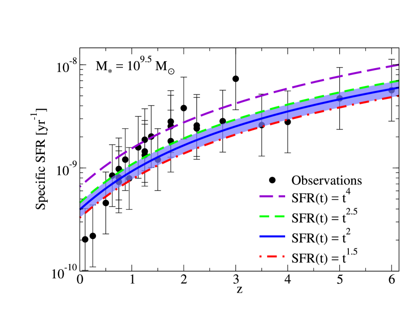
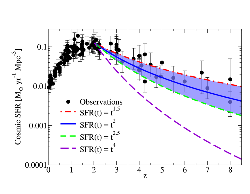
Figure 43: Illustrations of tension between observed SSFRs and the evolution of SMFs and CSFRs. Top panel shows observed average SSFRs (Appendix C.3) for galaxies with $M_{\ast}\sim 10^{9.5}\;\mathrm{M}_{\odot}$. Overlaid are predictions for average SSFRs (including effects of stellar mass loss) for different power-law star formation histories. The blue shaded region shows a very generous interpretation of current constraints on galaxy star formation histories at $z\sim 2$ (Papovich et al., 2011; Behroozi et al., 2013e). Nonetheless, most observations are $\sim 0.3$ dex higher. As discussed in the text, this would imply a typical $t^{4}-t^{5}$ star formation history, which would have drastic consequences for, e.g., the evolution of SMFs and CSFRs (bottom panel).

C.4 Tension Between SMFs and SSFRs

Tensions between integrated SFRs and the evolution of SMFs have been repeatedly noted, especially at $z\sim 2$ (Hopkins & Beacom, 2006; Wilkins et al., 2008; Leja et al., 2015; Yu & Wang, 2016). Given current systematic uncertainties on stellar masses and SFRs ($\sim 0.3$ dex), it is possible to find self-consistent solutions that approximately match all data sets (e.g., Moster et al., 2013; Behroozi et al., 2013e). The source of these tensions has remained unclear, but major factors include a lack of calibration data for SFR indicators (e.g., radio and 24$\mu$m) at higher redshifts, as well as the fact that star formation history priors for stellar mass fits are not fully self-consistent with SMF evolution. Examples of this at $z>4$ are discussed in Appendix D. Here, we show explicitly how this affects $z\sim 2$ SSFRs.

Low-mass galaxies at $z\sim 2$ are still rapidly increasing in stellar mass, with the evolution of stellar mass and luminosity functions giving typical star formation histories of $t^{1.7}$ (Papovich et al., 2011) to $t^{2}$ (Behroozi et al., 2013e). For a given power-law star formation history, $SFR(t)\propto t^{n}$, the ratio of the SFR to total stellar mass formed is:

$$SSFR_{\mathrm{total}}(t)=\frac{n+1}{t}.$$ (37)

Returned stellar mass ($<30\%$) will increase this; a slightly smaller effect is averaging log-normal scatter in observed SFRs at fixed SM ($\sim 0.3$ dex scatter results in a mean SSFR that is $27\%$ higher than the median). Combined, these corrections mean that $SSFR_{\mathrm{obs}}(t)<1.8\frac{n+1}{t}$. These observed SSFR predictions are overplotted on observations of $M_{\ast}\sim 10^{9.5}\;\mathrm{M}_{\odot}$ galaxies (Appendix C.3). Even for an overly generous range of possible star formation histories ($t^{1.5}$ to $t^{2.5}$), most observed SSFRs at $z=2$ are $\sim 0.2-0.3$ dex above the reasonable range (Fig. 43, top panel).

Because SSFRs are proportional to the index $n+1$, the observations at face value would imply $t^{4}-t^{5}$ star formation histories for typical low-mass galaxies at $z=2$. This steep history is inconsistent with both the evolution in SMFs and with CSFRs (Fig. 43, bottom panel). Hence, we adopt a parameter ($\kappa$, Eq. 26) to allow for discrepancies between SFRs and SMs that peaks at $z\sim 2$ and smoothly falls to nearly zero by $z=0$ and $z=4$.

C.5 UV Luminosity Functions

We adopt the UV luminosity functions of Finkelstein et al. (2015a) from $z=4$ to $z=8$, and the Bouwens et al. (2016a) luminosity functions for $z\sim 9$ and $z\sim 10$. As both studies use similar fields, the Finkelstein et al. (2015a) results are preferable at low redshifts due to the fact that they use photo-$z$ selection instead of LBG selection, and are hence easier to model. In addition, they are consistently selected with the galaxies that constrain our UV–stellar mass relations (Appendix D). On the other hand, the Finkelstein et al. (2015a) data do not extend to $z>8$, and so we adopt the Bouwens et al. (2016a) constraints at higher redshifts, approximating the LBG cuts as window functions ($z=8.4-9.5$ and $z=9.5-11$, at $z\sim 9$ and $z\sim 10$, respectively).

C.6 Quenched Fractions

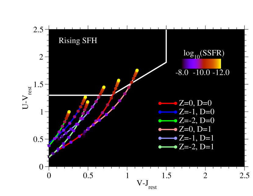
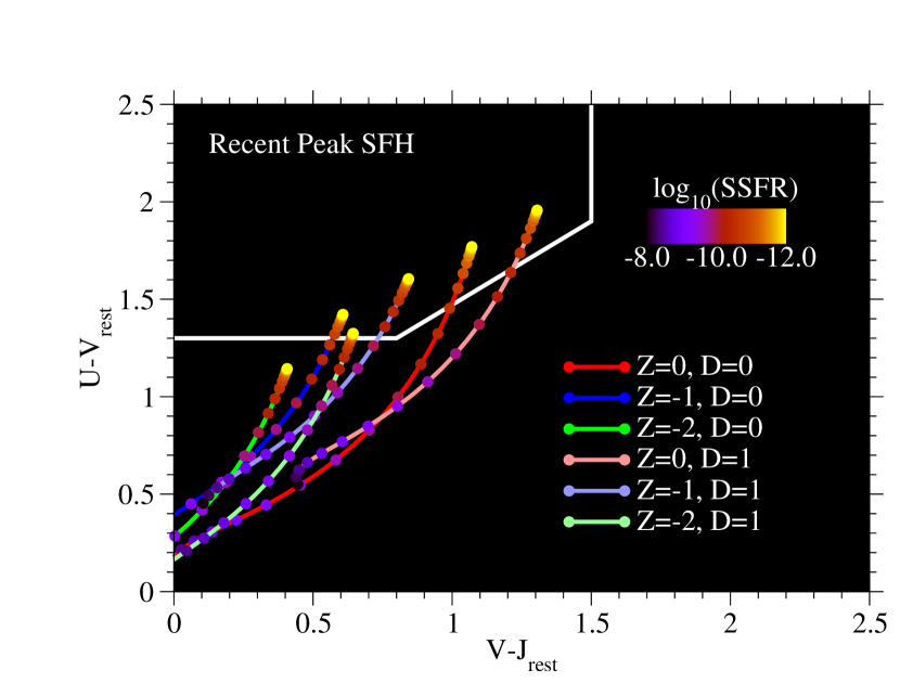
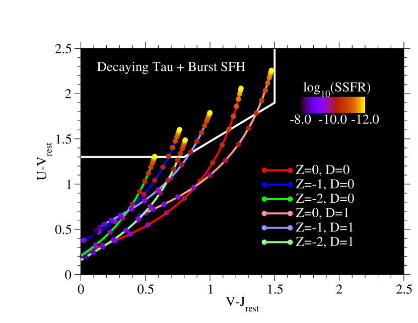
Figure 44: Galaxy position in the UVJ quenching diagram as a function of recent SSFR; different panels show the effects of different past star-formation histories (see text). Different line colours correspond to different stellar metallicities (0.01 solar to solar); different line saturations correspond to different dust prescriptions (D=0 implies no dust; D=1 implies Charlot & Fall 2000 dust). With some exceptions for low-metallicity / low-dust galaxies, the UVJ diagram separates quenched from star-forming galaxies at similar SSFRs.

Constraints on galaxy quenched fractions as a function of stellar mass (QFs) are taken from Bauer et al. (2013), Moustakas et al. (2013), Muzzin et al. (2013). Each paper has a different definition of “quenched,” so we calculate QFs in three different ways to compare as directly as possible to the observations. We computed the quenched fraction at $z\sim 0$ from the raw Bauer et al. (2013) data, defining “quenched” as an observed SSFR below $10^{-11}$ yr^-1.

When comparing to Moustakas et al. (2013) QFs, we use their adopted quenched/star-forming cut on the observed SSFR:

$$\log_{10}(SSFR_{q}\cdot\mathrm{yr})=-10.49-0.35\log_{10}\left(\frac{M_{\ast}}{10^{10}\;\mathrm{M}_{\odot}}\right)+1.07(z-0.1).$$ (38)

We excluded Moustakas et al. (2013) data at $z\sim 0$, because the SSFR cut for massive $10^{12}\;\mathrm{M}_{\odot}$ galaxies ($\sim 10^{-11.2}$) was lower than could be reliably measured, resulting in a spuriously low quenched fraction for such galaxies.

When comparing to QFs in Muzzin et al. (2013), we use their adopted cut in UVJ colour space (see also Labbé et al., 2005; Williams et al., 2009), specifically:

$$U-V>1.3,\,V-J<1.5\,$$ [all redshifts] (39)

$$U-V>(V-J)\times 0.88+0.69 \textrm{[0.0}<z<\textrm{1.0]}$$ (40)

$$U-V>(V-J)\times 0.88+0.59 \textrm{[1.0}<z<\textrm{4.0]}.$$ (41)

Muzzin et al. (2013) also explored the systematic errors arising from the UVJ cut location, and found that it may lead to $\sim 10\%$ differences in the resulting quenched fraction; we adopt $\pm 5\%$ systematic errors here.

When comparing to colour-based cuts, a caveat is that the choice of metallicity and dust can strongly affect galaxy luminosities. Since metallicity and dust are not treated self-consistently for the modeled galaxies, it is important to check whether incorrect metallicity / dust could significantly affect resulting quenched fractions. We generated three sets of star formation histories (rising, recent peak, and decaying tau) as a function of scale factor ($a$) according to the following equations for $0<a<1$:

$$SFH(a)\propto a^{2}$$ [rising] (42)

$$SFH(a)\propto a^{2}\exp(-4a)$$ [recent peak] (43)

$$SFH(a)\propto a^{3}\exp(-10a) \textrm{[decaying tau]}.$$ (44)

Then, for each initial history above, we generated 41 new star formation histories by substituting the last 300 Myr of the initial history with a constant SSFR between $10^{-12}$ yr^-1 and $10^{-8}$ yr^-1. We generated colours for each of these histories using FSPS with three different metallicity assumptions (solar, 0.1 solar, 0.01 solar) and two different dust assumptions (no dust, Charlot & Fall 2000 dust). This test allows us to see how well the UVJ diagram captures a recent change in the SSFR given a wide range of assumptions about the older stellar population history, the metallicity, and the dust.

Several trends are apparent in the results (Fig. 44). Galaxies with older pre-existing stellar populations (e.g., the decaying tau SFHs) require less recent star formation to exit the UVJ quenched box, so position in the UVJ diagram does not translate uniquely to SSFR. However, for a fixed star formation history, galaxies with solar metallicities and dusty low-metallicity galaxies (0.1 solar) all enter the quenched box in the UVJ diagram at similar SSFRs. As these galaxies make up the majority of quenched galaxies in the Universe (Muzzin et al., 2013), this would suggest that modest inaccuracies in assumptions about metallicity and dust will not affect the resulting quenched fraction as long as the underlying star formation history is correct. That said, low-metallicity, low-dust galaxies with rising star formation histories could lie below traditional quenched boxes (Fig. 44, upper panel); and similarly, extremely dusty galaxies with very old populations (Fig. 44, lower panel) could lie to the right of traditional quenched boxes. This suggests that the present vertical and horizontal boundaries used (Eq. 39) are artificial and might be better removed or significantly relaxed as, e.g., $U-V>0.8$ and $V-J<1.7$.

C.7 Galaxy Correlation Functions and Covariance Matrices

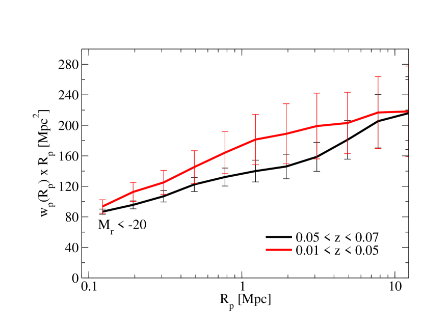
Figure 45: Excess clustering in the SDSS at $z<0.05$ for an autocorrelated luminosity threshold sample ($M_{r}<-20$) as compared to higher redshifts. Errors shown here are from 16 jackknife bins.

Table 8: Measured Correlation Functions from the SDSS

$M_{\ast}^{\mathrm{min}}$	$M_{\ast}^{\mathrm{max}}$	$z_{\mathrm{min}}$	$z_{\mathrm{max}}$	$V/$Gpc3	N	$f_{\mathrm{SF}}$
$10^{10.3}\;\mathrm{M}_{\odot}$	$10^{10.5}\;\mathrm{M}_{\odot}$	0.045	0.069	0.012	10081	0.51
$10^{10.5}\;\mathrm{M}_{\odot}$	$10^{11.0}\;\mathrm{M}_{\odot}$	0.045	0.070	0.013	16953	0.40
$10^{11.0}\;\mathrm{M}_{\odot}$	$10^{13.0}\;\mathrm{M}_{\odot}$	0.090	0.121	0.050	16912	0.29

Galaxy correlation functions (CFs) for all, quenched, and star-forming galaxies are derived from the SDSS DR7 (Abazajian et al., 2009). Stellar masses and star formation rates were taken from the public catalogues of Kauffmann et al. (2003) and Brinchmann et al. (2004), respectively, as updated for DR7. Stellar masses were translated to match the adjusted Moustakas et al. (2013) SMF (Appendix C.2) by abundance matching at fixed cumulative number density to the SDSS DR7 SMF in Behroozi et al. (2015a); the resulting offsets were $<$0.03 dex for all stellar mass bin edges up to $10^{11}\;\mathrm{M}_{\odot}$, consistent with findings in D’Souza et al. (2015). Although both Brinchmann et al. (2004) and Bauer et al. (2013) SFRs are H$\alpha$-based, we found modest discrepancies. To match the quenched fraction inferred from Bauer et al. (2013) (using a cut of SSFR$<10^{-11}$ yr^-1), we found that we had to apply a quenched threshold of SSFR$<10^{-11.3}$ yr^-1 in the data from Brinchmann et al. (2004).

We first generate volume-limited catalogues in each mass bin according to the cut in Behroozi et al. (2015a):

$$-0.25-1.9\log_{10}\left(\frac{M_{\ast}}{\;\mathrm{M}_{\odot}}\right)+5\log_{10}\left(\frac{D_{L}(z)}{10\mathrm{pc}}\right)<17.77.$$ (45)

We then calculate the two-point 3D CF $\xi(r_{p},\pi)$ out to $\pi=\pm 20$ Mpc (comoving) in bins of $1$ Mpc in $\pi$ using the Landy & Szalay (1993) estimator ($\xi=(DD-2DR+RR)/RR$) with 10⁶ randoms distributed with constant number density over the same angular (6261.75 deg²) and redshift footprint. For cross-correlations, we use the modified estimator $\xi=(D_{1}D_{2}-D_{1}R_{2}-D_{2}R_{1}+R_{1}R_{2})/R_{1}R_{2}$, which reduces to the Landy & Szalay (1993) estimator for autocorrelations.

We then integrate $\xi$ along the line-of-sight direction ($\pi$) to obtain $w_{p}(r_{p})$. The limited line-of-sight integration is necessary because several CFs are calculated over narrow redshift slices ($<100$ Mpc), so longer integrations in $\pi$ would not be possible for the majority of the galaxies. No correction is required, however, as we perform the identical integration on the generated mock galaxy catalogues when comparing to data. As is typically done (Skibba et al., 2014) for galaxies at redshift-space positions $\mathbf{x}_{1}$ and $\mathbf{x}_{2}$, we define:

$$\mathbf{s}=\mathbf{x}_{1}-\mathbf{x}_{2}, \mathbf{l}=0.5(\mathbf{x}_{1}+\mathbf{x}_{2})$$ (46)

$$\mathbf{\pi}\equiv(\mathbf{s}\cdot\mathbf{l})/|\mathbf{l}|, r_{p}\equiv\sqrt{s^{2}-\pi^{2}}.$$ (47)

We correct for fiber collisions by weighting galaxy counts. Briefly, some areas of the SDSS were observed multiple times, with the result that for every observed pair within the fiber collision radius (55"), 2.08 galaxies have an unobserved pair (Patton et al., 2013). For each such galaxy pair, we therefore add each of their individual contributions to the $DD$ counts 1.04 extra times to account for collided galaxies not present in the spectroscopic sample. At large separations ($>100$ kpc for $M_{\ast}<10^{11}$ galaxies and $>200$ kpc for $M_{\ast}>10^{11}\;\mathrm{M}_{\odot}$ galaxies), the change in $w_{p}(r_{p})$ is $<5\%$. We do not attempt to calculate $w_{p}(r_{p})$ at closer separations, partially as much more sophisticated algorithms are necessary to robustly recover $w_{p}$ (e.g., Guo et al., 2015).

Table 8 lists the redshift and stellar mass bins we use for measuring autocorrelation functions. We additionally measure the cross-correlation between galaxies with $M_{\ast}>10^{11}\;\mathrm{M}_{\odot}$ and galaxies with $10^{10.3}\;\mathrm{M}_{\odot}<M_{\ast}<10^{10.5}\;\mathrm{M}_{\odot}$, in the same redshift bin as for the $10^{10.3}\;\mathrm{M}_{\odot}<M_{\ast}<10^{10.5}\;\mathrm{M}_{\odot}$ autocorrelation function. Redshift bin constraints arise from volume completeness requirements, SDSS Great Wall avoidance ($0.07<z<0.09$; Gott et al. 2005), and a $1-2\sigma$ clustering excess at $z<0.045$. The clustering excess is shown in Fig. 45; the excess is robust to choice of luminosity or stellar mass bin, choice of stellar masses (e.g., from Blanton et al. 2005), method of distributing randoms (e.g., randomizing sky position of galaxies instead of assuming constant number density, correcting for redshift-space distortions in volume density), local flow corrections (e.g., Tonry et al., 2000), method of counting randoms (e.g., direct pair counts or Monte Carlo integration), and method for computing $\mathbf{\pi}$ or $r_{p}$ (e.g., sky angle times mean distance).

Covariance matrices are crucial when comparing modeled to observed CFs, as CF bins are often extremely covariant. We compute covariance matrices for the observations by generating mock lightcones from the MDPL2 simulation at the mean redshifts of the samples in Table 8; notably, this simulation did not include orphan galaxies. Stellar masses were assigned by abundance-matching the $z\sim 0.1$ SMF from Appendix C.2 to haloes on $v_{\mathrm{Mpeak}}$ with $0.2$ dex of log-normal scatter (following Reddick et al. 2013). Quenching was correlated with $\Delta v_{\mathrm{max}}$ (Eq. 1) with $r_{c}=0.7$ (§3.2), with the fraction of galaxies varying as a function of $v_{\mathrm{Mpeak}}$ according to Appendix 53. For each sample in Table 8, 5000 mock lightcones were generated with the same footprint as the SDSS DR7, and auto- and cross CFs for all, quenched, and star-forming galaxies were calculated using the identical code used to calculate observed auto- and cross CFs. Matrices for the simultaneous covariance of all, quenched, and star-forming galaxies were computed, with $N_{\mathrm{bins}}=24-39$ for each sample in Table 8. For model covariance matrices, the observed volume is much smaller than the volume of Bolshoi-Planck for the two lower-mass bins in Table 8, so we assume that the model covariance matrices are subdominant to the observed ones. For the highest-mass bin, we assume that the model covariance matrix is equivalent to the observational covariance matrix, as the observational and simulated volumes are nearly equal.

Computing covariance matrices requires a volume $\sim 10\times V_{\mathrm{obs}}\times N_{\mathrm{bins}}$ for the resulting error estimates to be accurate at the $\sim 10\%$ level (Dodelson & Schneider, 2013). Our largest available high-resolution simulation (MDPL2) has a volume of 3.22 Gpc³. This volume is appropriate for the two lower-mass samples in Table 8, but likely is oversampled for the highest-mass bin. To investigate this, we performed a Principal Component (PC) Analysis on all covariance matrices to obtain PCs ($\mathbf{PC}_{1}$…$\mathbf{PC}_{n}$) and their corresponding standard deviations ($\sigma_{1}\ldots\sigma_{n}$). For the highest-mass sample, only 7 PCs have standard deviations of $>10\%$; the volume of MDPL2 suggests that we should trust the largest $\sim 3.22$ Gpc${}^{3}/(10V_{\mathrm{obs}})=6$ PCs. However, we note that systematic errors inherent in calculating CFs (including errors in modeling fiber collisions, edge effects, systematic variations in photometry across the sky, different typical colours of central vs. satellite galaxies leading to different systematic stellar mass offsets) set a maximum achievable accuracy of no better than 10%. Hence, for all samples, we take the effective error on the $i$th PC to be $\sigma_{\mathrm{eff},i}\equiv\max(10\%,\sigma_{i})$. The resulting contribution ($\Delta\chi^{2}$) to the total error calculation from a given correlation function then becomes:

$$\Delta\chi^{2}=\sum_{i=1}^{n}\left(\frac{\mathbf{PC}_{i}\cdot(\mathbf{w}_{p,\mathrm{obs}}-\mathbf{w}_{p,\mathrm{model}})}{\sigma_{\mathrm{eff},i}}\right)^{2}.$$ (48)

Results for the measured auto- and cross correlation functions are shown in Fig. 5.

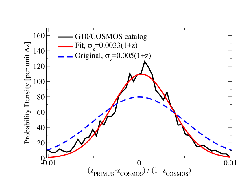
Figure 46: Comparison between redshifts in the G10/COSMOS catalogue (Davies et al., 2015) and the PRIMUS DR1 catalogue (Coil et al., 2011). This test suggests that the original redshift errors reported in Coil et al. (2011) overestimate the true redshift errors in PRIMUS.

At $z>0$, we adopt the PRIMUS correlation functions from Coil et al. (2017). Of the reported correlation functions, only one mass bin ($10^{10.5}\;\mathrm{M}_{\odot}<M_{\ast}<10^{11}\;\mathrm{M}_{\odot}$ at $0.2<z<0.7$) is complete and has both star forming and quenched samples available. Covariance matrices for this data were generated in the same way as for the SDSS (i.e., from MDPL2, using a lightcone with a footprint matching the observed angular area). Tests on these mock lightcones revealed that it was not possible to match the observed PRIMUS clustering amplitudes with reported redshift errors (Coil et al., 2011) of $\sigma_{z}=0.005(1+z)$. Cross-comparing redshifts between the PRIMUS DR1 catalogues and the G10/COSMOS catalogues (Davies et al., 2015) revealed much lower typical errors of $\sigma_{z}=0.0033(1+z)$, as shown in Fig. 46. We therefore adopt this lower estimate of the redshift errors when comparing to the Coil et al. (2017) data.

C.8 Environmental Dependence of Central Galaxy Quenching

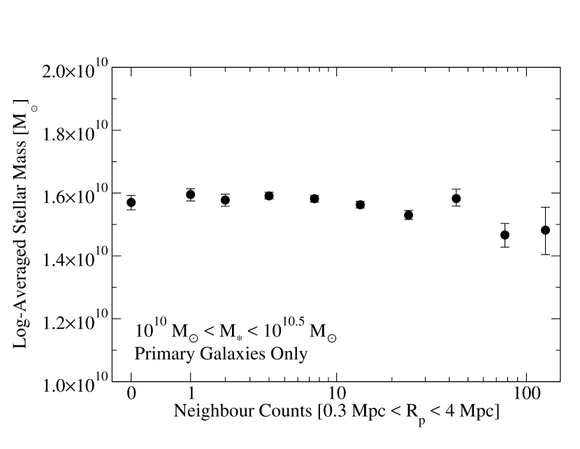
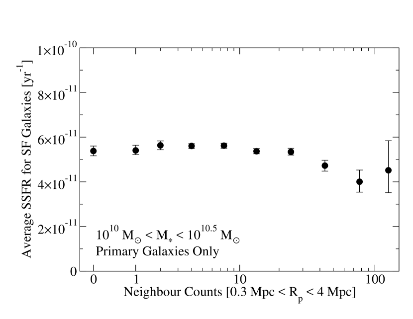
Figure 47: Top panel: average stellar mass of primary galaxies as a function of neighbour count, showing that the chosen environment proxy does not bias the stellar mass distribution. Bottom panel: average specific SFR for star-forming primary galaxies as a function of environment.

Even though satellites make up a small fraction of galaxies ($\lesssim 30\%$ for $M_{\ast}>10^{10}\;\mathrm{M}_{\odot}$; Reddick et al. 2013), correlation functions (CFs) weight galaxies by density. This results in satellites dominating the CF signal to large distances; well into the traditional 2-halo regime, there are significant contributions from satellite-central pairs and satellite-satellite pairs with different host haloes. As a result, CFs of star-forming and quenched galaxies provide an excellent constraint on satellite quenching, but are less useful for constraining central galaxy quenching. Lensing of star-forming and quenched galaxies has a similar problem, as increasing the satellite fraction will boost the shear signal significantly. Hence, higher-order statistics that explicitly exclude satellites are required to test quenching models for central galaxies.

The most well-known such statistic is two-halo conformity (Kauffmann et al., 2013)—i.e., the correlation between SSFRs for central galaxies separated by up to 4 Mpc (projected). Two-halo conformity plausibly arises because of correlations between galaxy assembly history and environment (Hearin et al., 2015, 2016). As galaxies share similar environments on large scales (evidenced by $\sigma_{8}\sim 1$), central galaxy quenching is spatially correlated.

Two-halo conformity thus measures a very indirect correlation (galaxy 1’s SSFR $\leftarrow$ environment $\rightarrow$ galaxy 2’s SSFR), and this has resulted in significant debate about its existence (e.g., Sin et al., 2017; Treyer et al., 2018). Here, we achieve much better signal/noise for the same data by measuring the direct dependence of the quenched fraction of central galaxies on environment.

To this end, we select $10^{10}\;\mathrm{M}_{\odot}<M_{\ast}<10^{10.5}$ galaxies from the SDSS DR7 over the redshift range $0.01<z<0.057$, using the same stellar masses and star formation rates discussed in Appendix C.7. To select primarily central galaxies ($\equiv$ primary galaxies), we exclude galaxies with larger (in stellar mass) neighbours within 500 kpc in projected distance and 1000 km s^-1 in redshift; we also excluded those near bright cluster galaxies lacking spectra as discussed in Behroozi et al. (2015a). Tests on mock catalogues suggest that this selection has a purity of 97.4% and a completeness of 77% for central galaxies (Behroozi et al., 2015a). We define environment as the number of neighbouring galaxies within 0.3 to 4 Mpc (i.e., in an annulus excluding satellites) in projected distance, 1000 km s^-1 in redshift, and with stellar masses between $0.3-1$ times the mass of the central galaxy. Without this cut on stellar mass, larger galaxies would preferentially have many more neighbours due to their higher bias. As detailed in Behroozi et al. (2015a), we weight galaxies by the inverse observable volume of their dimmest potential neighbours using Eq. 45, and we exclude galaxies whose dimmest potential neighbours are not observable.

Results are shown in Fig. 8. As a basic test of the selection technique, we also show that our environmental measure does not correlate with the stellar mass of the central galaxy (Fig. 47, top panel). We note in passing that SSFRs of star-forming galaxies change relatively little as a function of environment (Fig. 47), suggesting (as in Wetzel et al. 2013 and Berti et al. 2017) a rapid transition from being star-forming to being quiescent.

Appendix D Deriving UV–Stellar Mass Relations at z>4

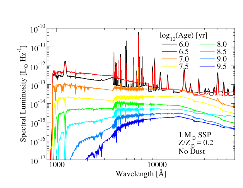
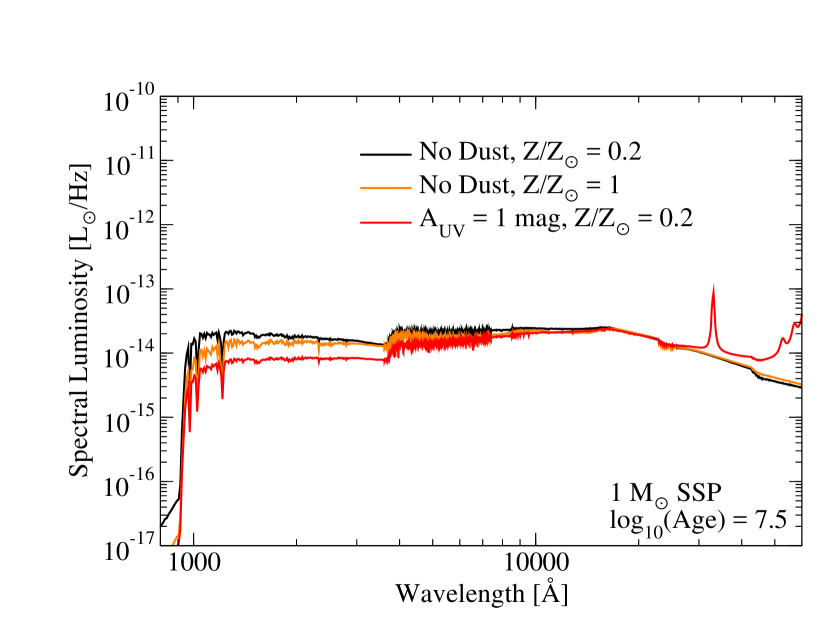
Figure 48: Top: Spectral luminosity (i.e., the spectral energy distribution) for a 1$\;\mathrm{M}_{\odot}$ single stellar population (SSP), with nebular emission, no dust, and 0.2 solar metallicity. Population age results in significant mass/light ratio variations. Bottom: Spectral luminosity for a 1$\;\mathrm{M}_{\odot}$ SSP, varying dust and metallicity. While mass/light ratio variations are significantly less, broadband spectral features sensitive to age (e.g., UV slopes) also depend on dust and metallicity. All spectra from FSPS (Conroy et al., 2009), with a Chabrier (2003) IMF.

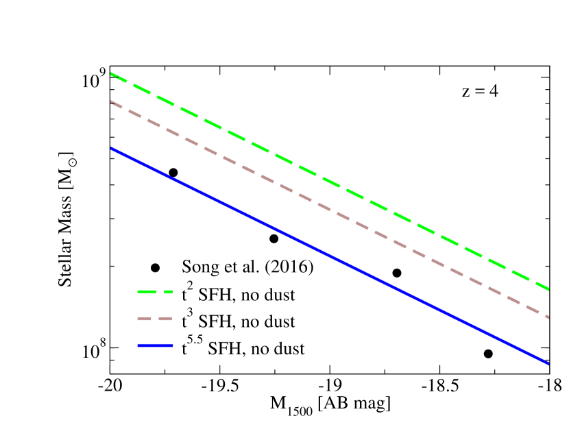
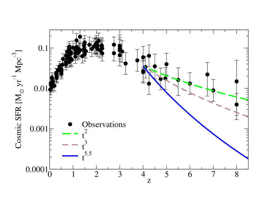
Figure 49: Top: The Song et al. (2016) UV–stellar mass relation at $z=4$ (from median stacks), compared with expected UV–stellar mass relations for low-metallicity ($Z/Z_{\odot}=0.03$) SFHs with no dust from FSPS (Conroy et al., 2009). At low luminosities, the Song et al. (2016) relation is best fit by a very steep $t^{5.5}$ SFH—requiring very short timescales for star formation. Adding dust or metallicity would require even steeper SFHs to compensate; using Bruzual & Charlot (2003) instead of FSPS has minimal effect ($<$0.06 mag). Bottom: growth rate of the cosmic star formation rate for several different power-law SFHs. If galaxies typically had $t^{5.5}$ or similar SFHs at $z=4$, observed CSFRs would be very different at high redshifts. More reasonable typical SFHs of $t^{2}$ (Papovich et al., 2011; Behroozi et al., 2013e; Salmon et al., 2015) would result in 0.3 dex larger inferred masses at a given UV luminosity (see top panel). Notes: Song et al. (2016) results are converted to a Chabrier (2003) IMF to match analysis here.

Table 9: Stellar Mass Fitting Models.

Legend (Fig. 50)	SFH	$\alpha$-prior	Burst	Dust	Dust Prior	$Z$ prior
Pure Power-law SFHs
$0<\alpha<4$; ALMA dust∗	$t^{\alpha}$	$0<\alpha<4$	no	1c	Bouwens et al. (2016b)	Maiolino et al. (2008)
$0<\alpha<4$; no dust prior	$t^{\alpha}$	$0<\alpha<4$	no	1c	none	Maiolino et al. (2008)
$0<\alpha<4$; ALMA dust; Free Z	$t^{\alpha}$	$0<\alpha<4$	no	1c	Bouwens et al. (2016b)	Maiolino et al. (2008) + arb. offset
$0<\alpha<10$; no dust priors	$t^{\alpha}$	$0<\alpha<10$	no	1c	none	Maiolino et al. (2008)
Power-law + 20 Myr Burst SFHs
$0<\alpha<10$; no dust prior	$t^{\alpha}$ + burst	$0<\alpha<10$	20 Myr	1c	none	Maiolino et al. (2008)
$0<\alpha<4$; 1c ALMA dust	$t^{\alpha}$ + burst	$0<\alpha<4$	20 Myr	1c	Bouwens et al. (2016b)	Maiolino et al. (2008)
$0<\alpha<4$; 2c ALMA dust	$t^{\alpha}$ + burst	$0<\alpha<4$	20 Myr	2c	Bouwens et al. (2016b)	Maiolino et al. (2008)
Power-law + Arbitrary-length Burst SFHs
$0<\alpha<10$; no dust prior	$t^{\alpha}$ + burst	$0<\alpha<4$	Arb.	1c	none	Maiolino et al. (2008)
$0<\alpha<4$; 2c ALMA dust	$t^{\alpha}$ + burst	$0<\alpha<4$	Arb.	2c	Bouwens et al. (2016b)	Maiolino et al. (2008)

Notes. 1c = 1-component dust (i.e., fixed optical depth for full SFH), 2c = 2-component SFH (i.e., different optical depth for younger stars, similar to Charlot & Fall 2000). “Bursts” are treated as periods of constant star formation at the end of the SFH. ^∗ denotes the fiducial model.

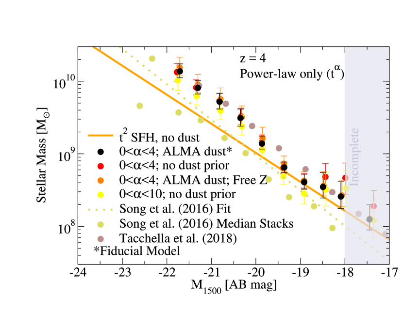
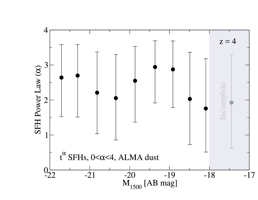
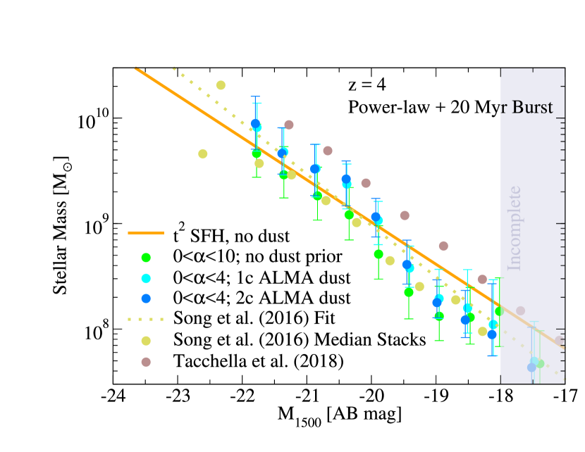
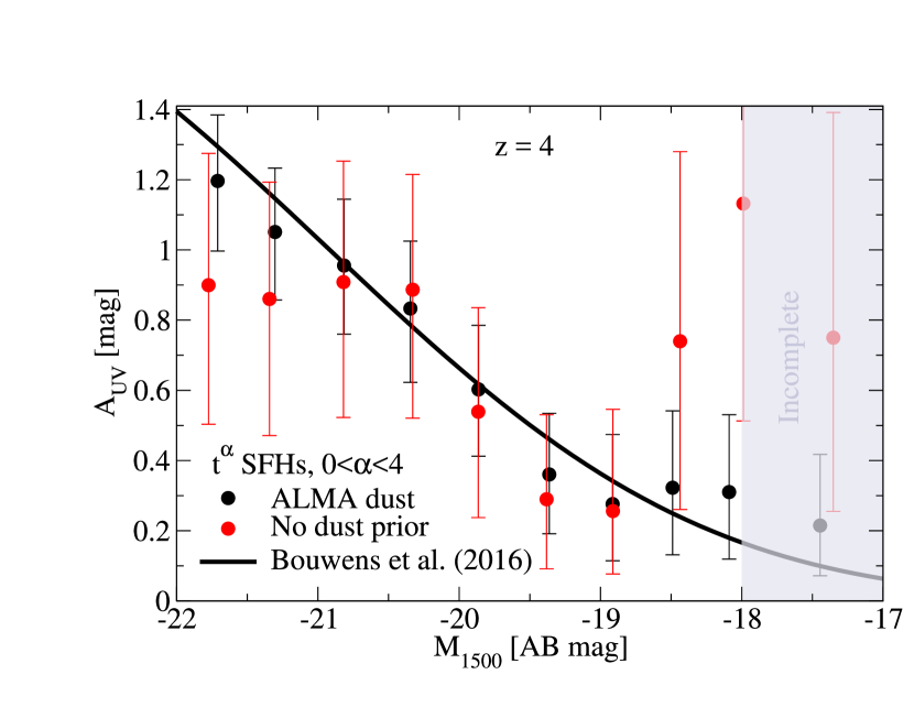
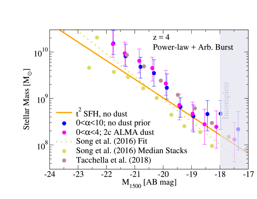
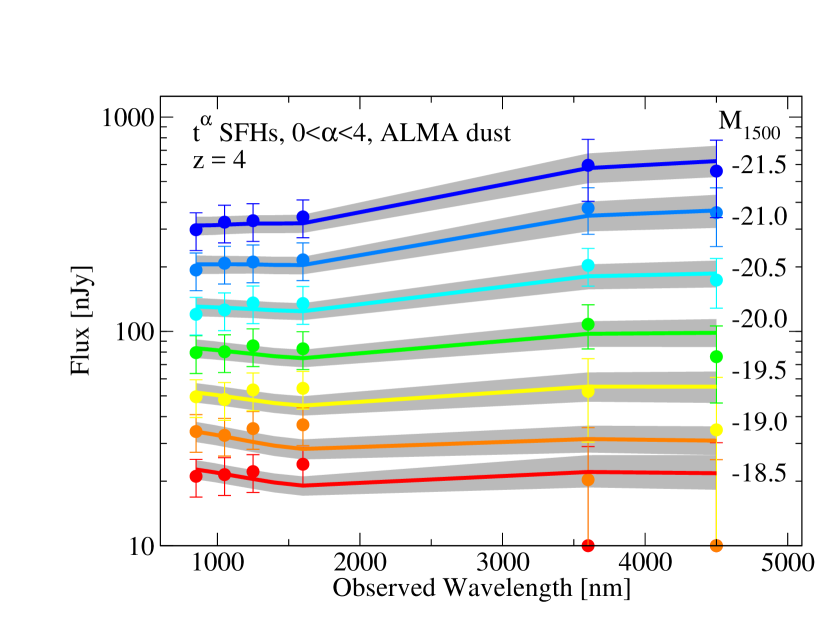
Figure 50: Left panels: Effects of priors and parameterizations (see Table 9 for full descriptions) on inferred mass-to-light ratios at $z=4$, based on fits to Song et al. (2016) SED stacks. Coloured points with error bars show the median and $68^{\mathrm{th}}$ percentile range of the posterior distributions for each prior/parameterization set. Coloured points without error bars show comparisons to median relations from Song et al. (2016) and Tacchella et al. (2018). Using pure power-law SFHs (top-left) or power-law SFH plus arbitrary-length bursts (bottom-left) gives higher mass-to-light ratios than using power-law SFHs with fixed 20 Myr bursts (middle-left panel). Top-right panel: inferred power-law index for galaxy SFHs. While constant SFHs are modestly disfavoured, the index is otherwise poorly constrained due to degeneracies, and it is hence heavily influenced by the prior. Middle-right panel: inferred total attenuation ($A_{UV}$) at $z=4$ with and without dust priors from Bouwens et al. (2016b). Inferred $A_{UV}$ values without dust priors are consistent with the Bouwens et al. (2016b) results except at low luminosities, where dust content is poorly constrained by the optical/near-infrared SEDs. Bottom-right panel: posterior distributions (grey bands; coloured lines are best-fitting results) for the broadband SED stacks from Song et al. (2016) (coloured points). Red UV slopes at faint luminosities are in modest tension with the low Spitzer flux and low dust emission inferred in Bouwens et al. (2016b). Light steel-blue shaded regions denote the luminosity completeness thresholds in Song et al. (2016). Notes: Song et al. (2016) and Tacchella et al. (2018) results are converted to a Chabrier (2003) IMF to match analysis here.

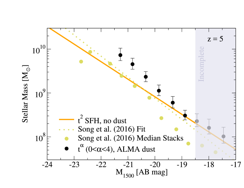
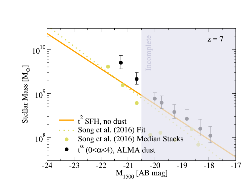
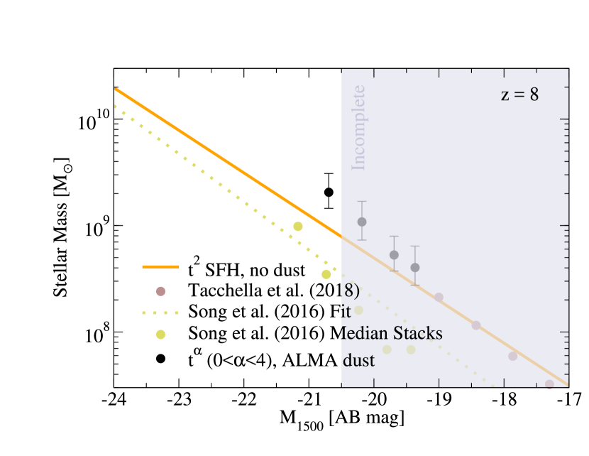
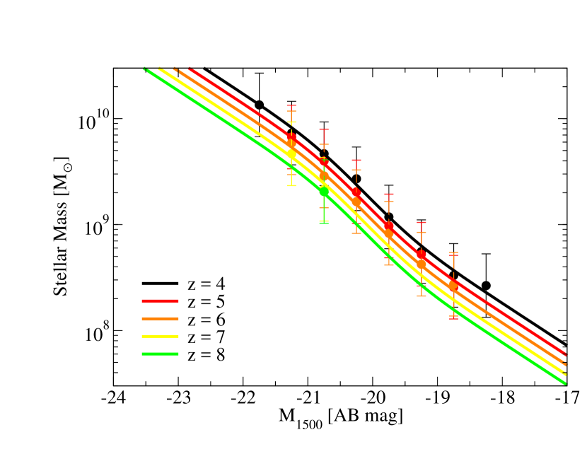
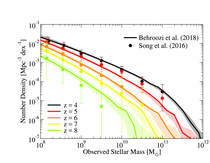
Figure 51: UV–stellar mass relations for $z=5$ to $z=8$ obtained from SEDition and the Song et al. (2016) SED stacks using fiducial priors ($t^{\alpha}$ SFHs with $0<\alpha<4$, dust priors from Bouwens et al. 2016b, and metallicity histories consistent with Maiolino et al. 2008). Black points with error bars show the median and $68^{\mathrm{th}}$ percentile range of the posterior distributions for the fiducial prior/parameterization set. Luminosity bins with fewer than 10 ($z=5$) or 5 ($z=6-8$) galaxies in Song et al. (2016) were not fit. coloured points without error bars show comparisons to median relations from Song et al. (2016) and Tacchella et al. (2018). Light steel-blue shaded regions denote the luminosity completeness thresholds in Song et al. (2016). Notes: Song et al. (2016) and Tacchella et al. (2018) results are converted to a Chabrier (2003) IMF to match analysis here. Tacchella et al. (2018) relations at $z=8$ are fully within the incomplete region.

Figure 52: Left panel: Fits (Eq. 53) to median UV–stellar mass relations for $z=4$ to $z=8$ obtained from SEDition. Right panel: $z=4-8$ stellar mass functions, derived from the UniverseMachine. Lines are the best-fitting model, and shaded regions show the $16^{\mathrm{th}}-84^{\mathrm{th}}$ percentile range of the posterior distribution. These principally depend on the UVLFs from Finkelstein et al. (2015a) and the UV–SM relations in the left panel (no $z\geq 4$ SMFs were used as input constraints). These are not significantly different from Song et al. (2016) except at $z=8$. Data for both panels is available online.

Converting light to stellar mass requires assumptions for photometry, redshift determinations, stellar population synthesis, star formation histories (SFHs), metallicities, dust amounts/sizes/geometries, and initial mass functions, introducing 0.3-0.5 dex systematic uncertainties (see Conroy & Gunn, 2010; Behroozi et al., 2010, for details). Determining stellar masses from broadband spectral energy distributions (SEDs) is especially difficult, as the main age-sensitive features are degenerate with dust, metallicity, and nebular emission. For example, while the UV slope depends on age (Fig. 48, top panel), it also depends on metallicity and dust (Fig. 48, bottom panel). The strength of the Balmer/4000Å breaks also depend on age, but a large broadband “break” can arise both from an old, dust-free population and from a dusty population of young (<10 Myr) stars with significant nebular emission. Due to these degeneracies, inferred mass-to-light ratios are very sensitive to priors on age, dust, and metallicity.

Flat priors, as used by many fitting codes, can lead to unphysical results. For example, the median UV–SM relation for $z\sim 4$ galaxies from Song et al. (2016) requires very low mass-to-light ratios, typical of recent burst or steeply rising star formation histories. Comparing the Song et al. (2016) relation to those for power-law SFHs, we find that $t^{5.5}$ or steeper SFHs are required to achieve similar mass-to-light ratios (Fig. 49), even with no dust and low metallicities. However, if typical galaxies had such steep SFHs, very different UVLF and CSFR evolution would result (e.g., Fig. 49, bottom panel; compare with Fig. 43). If SFHs that matched the CSFR evolution ($t^{2}$) or UVLF/SMF evolution at $z>4$ ($t^{1.4}-t^{2}$; Papovich et al. 2011; Behroozi et al. 2013e; Salmon et al. 2015) were used instead, the inferred stellar masses would be 0.3 dex higher at fixed UV luminosity (Fig. 49, upper panel). While binning on UV luminosity does select galaxies with younger stellar populations, even very steep $t^{3}$ SFHs would still result in 0.2 dex larger stellar masses.

The SED data available in Song et al. (2016) are nonetheless among the best currently published, as they include deep Spitzer observations that probe rest-frame optical colours. Hence, we re-fit the median SED stacks in Song et al. (2016) with empirical priors for dust, metallicity, and age to obtain more self-consistent stellar masses. To this end, we develop a new Bayesian SED-fitting code (SEDition, the Spectral Energy Distribution Inference Tool for Infrared/Optical Normalization). Briefly, the code relies on FSPS to generate broadband luminosities as a function of stellar age, metallicity, and dust (including nebular continuum and emission lines). These luminosities are combined with an affine MCMC algorithm (Goodman & Weare, 2010; Foreman-Mackey et al., 2013) to explore SFH, dust, and metallicity parameter space. The code’s two main features are the flexible inclusion of empirical priors on galaxy properties as well as the wide variety of built-in parameterizations for galaxy SFHs, dust histories, and metallicity histories.

The fiducial model used herein assumes a pure power-law SFH ($t^{\alpha}$, with $0<\alpha<4$), uniform optical depth (i.e., 1-component dust) with a Calzetti (2001) attenuation law and total $A_{UV}$ priors from Bouwens et al. (2016b). For the latter, we fit $A_{UV}(M_{1500})$ under the assumption of evolving dust temperatures (e.g., Béthermin et al., 2015):

$$A_{UV}(M_{1500})=1+\mathrm{erf}\left(\frac{M_{1500}+20.93}{-3}\right).$$ (49)

For metallicity histories, the fiducial model adopts the gas-phase metallicities of Maiolino et al. (2008) for star formation. Specifically, the metallicity of new stars is assumed to be the same as the observed gas-phase metallicity at the time of formation, which depends on redshift and the total remaining mass of previously-formed stars; we use a smooth fit to the Maiolino et al. (2008) relation for $\log_{10}(Z(M_{\ast},z))\equiv 12+\log_{10}(O/H)$:

$$\log_{10}(M_{0}(z)) = 11.22+0.47z$$ (50)

$$K_{0}(z) = 9.07-0.07z$$ (51)

$$\log_{10}(Z(M_{\ast},z)) = K_{0}(z)-0.086\left[\log_{10}\left(\frac{M_{\ast}}{M_{0}(z)}\right)\right]^{2}.$$ (52)

As in §3.4, we set a lower metallicity floor of $\log_{10}(Z/Z_{\odot})=-1.5$ to avoid unphysically low metallicities at high redshifts and low stellar masses. Besides this fiducial model, we test many other possible assumptions for SFHs, dust, and metallicities (Table 9).

For full details on the methods and data sources used for the SED stacks, see Song et al. (2016). Briefly, SEDs were median-stacked for CANDELS galaxies in redshift bins from $z=4$ to $z=8$ ($\Delta z=1$), and in rest-frame UV magnitude bins of 0.5 mag. Available data included nonuniform coverage of $B_{435}$, $V_{606}$, $i_{775}$, $I_{814}$, $z_{850}$, $Y_{098}$, $Y_{105}$, $J_{125}$, $JH_{140}$, and $H_{160}$ bands (see Table 1 of Finkelstein et al., 2015a, for details), as well as Spitzer $3.6\mu$m and $4.5\mu$m bands. Following Song et al. (2016), we exclude bands containing Ly$\alpha$ and bands for which $<50\%$ of galaxies had a detection. Further, we exclude bands containing the Lyman break, and we use a dust law that does not include the 2175 Å UV bump (i.e., Calzetti, 2001); such features are expected to be smoothed because the galaxy SEDs were not $k$-corrected to the same redshift prior to stacking (M. Song, priv. comm.). Finally, following Finkelstein et al. (2015a), we assumed minimum 20% photometric uncertainties, due to a combination of Poisson statistics, redshift errors, fitting errors, and stacking uncertainties.

Table 9 lists the different parameterizations and priors tried for fitting the Song et al. (2016) SED stacks. Most assumptions gave significantly higher mass-to-light ratios than Song et al. (2016), and were consistent with $t^{2}$ dust-free mass-to-light ratios for low-luminosity galaxies (Fig. 50, left panels). The largest impact came from changing the SFH parameterization. Between pure power-law SFHs, power laws with 20 Myr constant-SFR bursts, and power laws with arbitrary-length bursts, the SFHs with 20-Myr bursts had significantly lower mass-to-light ratios than the other two parameterizations (Fig. 50, left panels). Similarly, allowing very steep power-law SFHs ($t^{\alpha}$ with $0<\alpha<10$) resulted in lower mass-to-light ratios than our fiducial prior ($0<\alpha<4$). Indeed, while constant SFHs were modestly disfavoured, the SEDs gave very weak constraints on the steepness of the SFH (Fig. 50, upper-right panel). Hence, SFH parameter spaces biased toward younger ages gave lower mass-to-light ratios; as the Song et al. (2016) SFH parameter space included SFHs as short as 1 Myr, this could be one explanation for the lower mass-to-light ratios therein. Consistency with external SFH estimates from UVLF and SMF evolution was therefore primary motivation for our choice of fiducial SFH prior.

Changing the dust parameterization from 1-component (i.e., identical $A_{UV}$ for all stars) to 2-component (i.e., different $A_{UV}$ for recent stellar populations vs. older stellar populations as in Charlot & Fall 2000) made little difference, as did allowing metallicity to vary (Fig. 50, left panels). Including dust priors from ALMA measurements (Bouwens et al., 2016b) made little difference for bright galaxies, because they were consistent with SED-derived dust estimates (Fig. 50, middle-right panel). However, the ALMA priors reduced mass-to-light ratios for low-luminosity galaxies (Fig. 50, middle-right panel), possibly because of corresponding uncertainties in stacking Spitzer flux (Dan Stark, priv. comm.). As shown in the SED posterior distributions (Fig. 50, bottom-right panel), low-luminosity galaxies had somewhat red median UV slopes ($\beta<2$) and faint Spitzer fluxes, in modest tension with the lack of ALMA dust emission. Given that other studies have found blue median UV slopes in this luminosity range (e.g., Bouwens et al., 2014), we expect that including ALMA priors makes the mass estimates somewhat more realistic (i.e., less dust and lower mass-to-light ratios).

To summarize, our fiducial priors yield results consistent with external constraints on UVLF and SMF evolution, galaxy gas-phase metallicities, and ALMA dust measurements, but significantly different assumptions can still fit the stacked SEDs. We thus adopt the median of the posterior distribution from our fiducial priors (Fig. 50, upper-left panel, and Fig. 52), but we increase the errors to 0.3 dex for all bins as an estimate of the systematic errors inherent in our modeling assumptions. Additionally, we exclude luminosity bins with fewer than 10 galaxies ($z=4-5$) or 5 galaxies ($z=6-8$) to reduce the influence of Poisson variations, and we adopt the same UV luminosity completeness cuts as in Song et al. (2016). The resulting data points (Fig. 52) are available in electronic form online.

In the past, median UV–SM relations have been fit with single power-laws (e.g., González et al., 2011; Stark et al., 2013; Duncan et al., 2014; Salmon et al., 2015; Song et al., 2016). At $z>4$, brighter galaxies also have more dust attenuation on average (e.g. Bouwens et al., 2014), so all fits to date have resulted in steeper slopes than -0.4 (i.e., that expected for constant mass-to-light ratios). However, faint galaxies at $z>4$ have not to date shown significant dust attenuation (Bouwens et al., 2014, 2016b), so it is unphysical to expect a steep power-law to continue fainter than, e.g., $M_{UV}=-19$. We find that the following equation fits all our data well (Fig. 52) for $z=4$ to $z=8$:

$$\log_{10}(M_{\ast}(M_{1500})) = -0.4(M_{1500}-4.04+0.232z)$$ (53)

$$+0.189\mathrm{erf}(-20.11-M_{1500}).$$

As shown in Table 1, we also include the Bouwens et al. (2016b) estimates of dust attenuation as a direct model constraint. We allow for offsets between galaxies’ observed and true stellar masses (§3.5), and so a highly-offset “true” stellar mass for galaxies could remain consistent with UV luminosity functions and the “observed” relation between UV luminosity and stellar mass, provided there was a large amount of dust attenuation. Hence, the estimated constraint from Fig. 14 of Bouwens et al. (2016b) on infrared excess as a function of observed UV luminosity places strong limits on this degeneracy. We assume errors in the estimate that are the greater of $\pm 0.5$mag or the difference between the two provided dust temperature models.

In the main body of the paper, we forward-model the evolution of galaxies in dark matter haloes, determining which models can match both the observed UVLFs and median UV–SM relations. No $z>4$ SMFs are used as input constraints (see §2.2), so the posterior distributions for SMFs at $z>4$ are a nontrivial result. As shown in Fig. 52, we find SMFs largely in agreement with those from Song et al. (2016) from $z=4$ to $z=7$—our higher normalization for the median UV–SM relation is largely balanced by fewer galaxies skewing to very large stellar masses. At $z=8$, however, we find a significantly higher SMF; the resulting SMF evolution from $z=7$ to $z=8$ is more in line with UVLF evolution over the same redshift range (Finkelstein et al., 2015a) as compared to Song et al. (2016).

Appendix E Verifying Functional Forms

E.1 Quenched Fraction

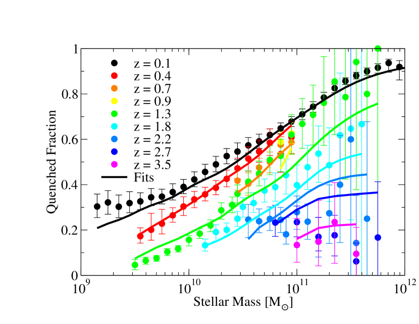
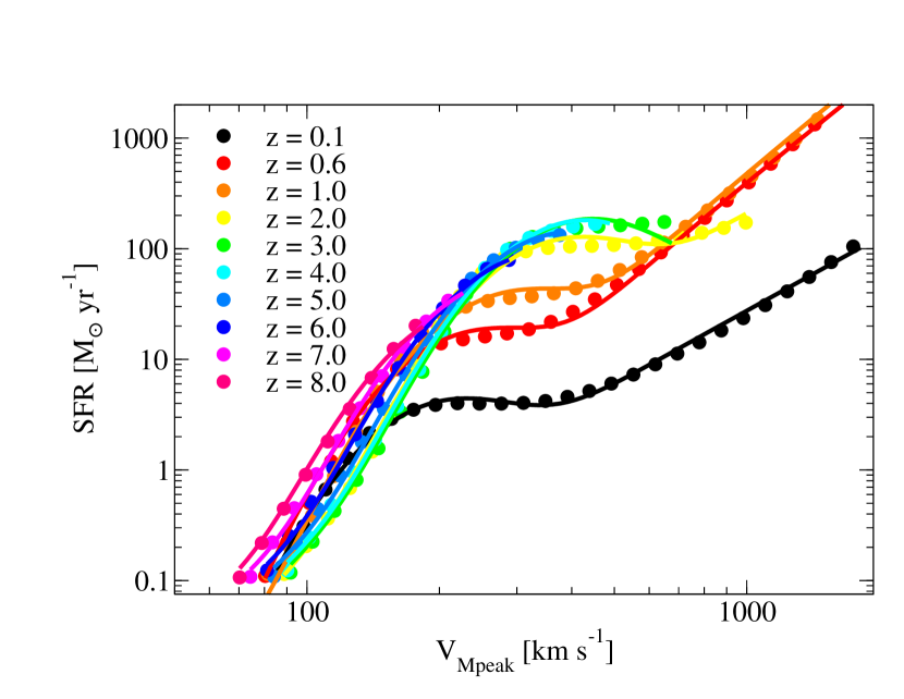
Figure 53: Top panel: test that the parametrization for $f_{\mathrm{Q}}(v_{\mathrm{Mpeak}},z)$ in Eqs. 12–15 (lines) is flexible enough to match the observed data (points) in Appendix C.6 (see Appendix 53). Bottom panel: test that the parametrization for $SFR_{\mathrm{SF}}$ in Eqs. 6–11 (lines) is flexible enough to match constraints from Behroozi et al. (2013e) (points), as discussed in Appendix E.2.

The quenched fraction as a function of $M_{\ast}$ is measurable directly (Appendix C.6), but the quenched fraction as a function of $v_{\mathrm{Mpeak}}$ is not. Yet, assuming that the scatter in $M_{\ast}$ at fixed $v_{\mathrm{Mpeak}}$ is not too correlated with SFR, the two are related by a convolution:

$$f_{\mathrm{Q}}(M_{\ast})=\int_{0}^{\infty}f_{\mathrm{Q}}(v_{\mathrm{Mpeak}})P(M_{\ast}|v_{\mathrm{Mpeak}})dv_{\mathrm{Mpeak}},$$ (54)

where $P(M_{\ast}|v_{\mathrm{Mpeak}})$ is the probability distribution of $M_{\ast}$ as a function of $v_{\mathrm{Mpeak}}$. Given that the quenched fraction is bounded between 0 and 1 and that it increases with stellar mass (and therefore increases with $v_{\mathrm{Mpeak}}$), it is natural to try a sigmoid function for $f_{\mathrm{Q}}(v_{\mathrm{Mpeak}})$, as in Eq. 12. We note that there may be an increase in the quenched fraction toward extremely low stellar masses (Wetzel et al., 2015); however, these are well below the halo mass resolution limit of the simulations we use.

We test the parametrization for $f_{\mathrm{Q}}(v_{\mathrm{Mpeak}},z)$ in Eqs. 12-15 via forward-modeling through Eq. 54 and comparing to the observed $f_{\mathrm{Q}}(M_{\ast},z)$ (Fig. 53, upper panel). Briefly, we obtain $P(M_{\ast}|v_{\mathrm{Mpeak}})$ at the median redshift of each stellar mass bin in Moustakas et al. (2013) and Muzzin et al. (2013) via abundance matching the corresponding SMFs to haloes rank-ordered by $v_{\mathrm{Mpeak}}$, with 0.2 dex scatter (matching Reddick et al. 2013). Any choice of parameters in Eqs. 14-15 fully specifies $f_{\mathrm{Q}}(v_{\mathrm{Mpeak}},z)$, from which Eq. 54 predicts the observed $f_{\mathrm{Q}}(M_{\ast})$. Using the standard likelihood function ($\exp(-0.5\chi^{2})$) and the emcee algorithm to explore parameter space (Foreman-Mackey et al., 2013), we find that Eqs. 12–15 are flexible enough to fit the observed data.

E.2 Star-formation Rates for Star-forming Galaxies

Constraints on $\langle SFR(M_{\mathrm{peak}},z)\rangle$ in Behroozi et al. (2013e) guide our functional form for $SFR_{\mathrm{SF}}(v_{\mathrm{Mpeak}},z)$. The median $v_{\mathrm{Mpeak}}$ as a function of halo mass and redshift in Bolshoi-Planck is

$$v_{\mathrm{Mpeak}}(M_{h},a) = 200\mathrm{km}\,\mathrm{s}^{-1}\left[\frac{M_{h}}{M_{200\mathrm{kms}}(a)}\right]^{3}$$ (55)

$$M_{200\mathrm{kms}}(a) = \frac{1.64\times 10^{12}\;\mathrm{M}_{\odot}}{\left(\frac{a}{0.378}\right)^{-0.142}+\left(\frac{a}{0.378}\right)^{-1.79}}.$$ (56)

Then, $\langle SFR\rangle$ and $SFR_{\mathrm{SF}}$ are related as

$$SFR_{\mathrm{SF}}(v_{\mathrm{Mpeak}},z)\approx C_{\sigma}\frac{\langle SFR(M_{\mathrm{peak}}(v_{\mathrm{Mpeak}},a),z)\rangle}{1-f_{\mathrm{Q}}(v_{\mathrm{Mpeak}},z)},$$ (57)

where $C_{\sigma}$ is a constant depending on the scatter in SFR at fixed $v_{\mathrm{Mpeak}}$; the equation is not exact due to very modest scatter ($<0.1$ dex) in $v_{\mathrm{Mpeak}}$ at fixed $M_{\mathrm{peak}}$. For $f_{\mathrm{Q}}$, we use the best fit from Appendix 53; the resulting estimate of $SFR_{\mathrm{SF}}$ is shown as filled circles in Fig. 53, bottom panel. As in Appendix 53, we use the emcee algorithm to explore parameter space, finding again that Eqs. 6–11 are flexible enough to fit constraints in Behroozi et al. (2013e). Notably, simpler parameterizations (including double power-laws) would not be sufficient, due to an extra bump in efficiency near the transition between low-$v_{\mathrm{Mpeak}}$ and high-$v_{\mathrm{Mpeak}}$ power laws.

Appendix F Code Implementation, Parallelization, and Scaling

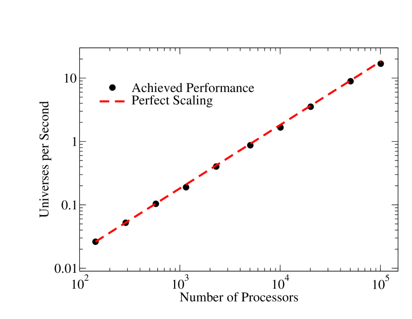
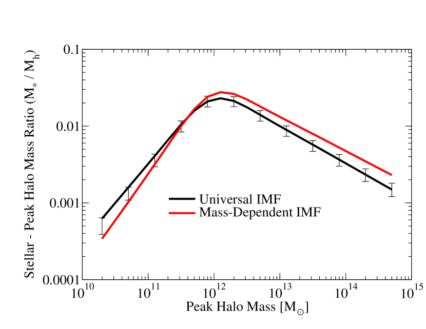
Figure 54: Strong scaling performance of the UniverseMachine code on Edison. Near-linear speedup with the number of processors is achieved.

Figure G1: Approximate effect of a mass-dependent IMF (Eqs. 58–61) on the stellar mass–halo mass relation at $z=0$. The error bars on the non-varying IMF model show 68% confidence intervals for other uncertainties in determining stellar masses.

The EmCee MCMC algorithm (Foreman-Mackey et al., 2013) is naturally parallelizable; we use a custom implementation in C. In this algorithm, multiple walkers (100–1000) simultaneously traverse parameter space, leapfrogging over each other to select new points to explore. No communication is required between walkers, with the result that each walker can be run on a different set of processors (or even on a different supercomputer) with near-perfect scaling (Fig. G1).

Each walker accepts a point in parameter space, populates haloes from the Bolshoi-Planck simulation with galaxies according to §3, and generates mock galaxy catalogues (i.e., containing locations, velocities, stellar masses, and SFRs). Since the halo catalogue for Bolshoi-Planck is $\sim$300 GB even in binary format (i.e., more than most single machines’ memory capacity), each walker divides the computations over 144 processors. Each processor handles a rectangular subvolume, pre-computed such that each processor generates galaxies for the same number of haloes. Processors work on each subvolume independently, processing haloes in chronological order. When a given processor finishes computation for haloes at a given timestep for its subvolume, it notifies neighbouring processors so that they may compute statistics (e.g., correlation functions) that require information outside their own subvolumes. To reduce sampling noise in the $\chi^{2}$ surface, simulated data is analytically convolved with observational errors (i.e., stellar mass, SFR, redshift, and photometric errors) for all observables. For two-point and higher-order correlations, all galaxies are weighted according to their net probability of being included in an observational bin. While this increases computational time per model evaluation, it also allows the use of gradient-based algorithms for finding the best fit as well as making an initial Fisher matrix-based guess for the initial walker distribution.

To reduce communication, average observables (e.g., the average SSFR for all galaxies, as opposed to the median SSFR) are used for constraints whenever possible. To reduce strain on the cluster I/O system when loading haloes, a Bittorrent-like method is employed, whereby walkers that have already loaded the data share it with others; thus, the data is loaded only once, and the achieved data throughput increases exponentially in time. At the time Fig. G1 was generated, each walker used 1.5 cpu-hours (36 wall-clock seconds; measured using Ivy-Bridge 2.4GHz processors on Edison) per point in parameter space to process the 2.3 billion haloes in Bolshoi-Planck. Recent improvements have lowered this to $0.8$ cpu-hours per point in parameter space. Source code and documentation are available at https://bitbucket.org/pbehroozi/universemachine.

Appendix G Non-Universal Initial Mass Functions

Many studies have found that the Initial Mass Function (IMF) becomes increasingly bottom-heavy at larger stellar velocity dispersions, although the exact amount and redshift dependence is debated (Conroy & van Dokkum, 2012; Conroy et al., 2013; Geha et al., 2013; Martín-Navarro et al., 2015; La Barbera et al., 2016; Posacki et al., 2015). van Dokkum et al. (2017) note that correcting for the radial gradient of the IMF significantly reduces these discrepancies. We can thus make a crude estimate of the effect of a mass-dependent IMF, starting with a stellar mass–$\sigma$ relation (Zahid et al., 2016):

$$\sigma(M_{\ast})=118.3\textrm{km s}^{-1}\left(\frac{M_{\ast}}{1.8\times 10^{10}\;\mathrm{M}_{\odot}}\right)^{\beta}$$ (58)

$$\beta=\begin{cases}0.403&\textrm{if }M_{\ast}<1.8\times 10^{10}\;\mathrm{M}_{\odot}\\ 0.250&\textrm{if }M_{\ast}\geq 1.8\times 10^{10}\;\mathrm{M}_{\odot}\end{cases}$$ (59)

where $\beta$ for $M_{\ast}\geq 1.8\times 10^{10}\;\mathrm{M}_{\odot}$ has been reduced by a factor 1.17; this accounts for our corrections to SDSS luminosities for massive galaxies (Appendix C.2; Fig. 41, middle panel). This is then combined with an IMF–$\sigma$ relation (Posacki et al., 2015):

$$\log_{10}(\alpha_{\mathrm{P15}})=0.38\log_{10}\left(\frac{\sigma}{200\textrm{km s}^{-1}}\right)+0.17,$$ (60)

where $\alpha_{\mathrm{P15}}$ is the mass-to-light ratio compared to that for a Chabrier (2003) IMF. We reduce the Posacki et al. (2015) $\alpha_{\mathrm{P15}}$ according to the aperture correction in van Dokkum et al. (2017) as

$$\alpha_{\mathrm{vD17}}=1+0.75(\alpha_{\mathrm{P15}}-1).$$ (61)

Perhaps coincidentally, Eq. 61 matches the IMF offset for ultrafaint dwarfs in Geha et al. (2013). Fig. G1 shows the resulting effect on the stellar mass–halo mass relation. This would suggest that IMF uncertainties remain substantial–as large as other modeling uncertainties combined. On the other hand, we note that none of the current observations used (Appendix C) are sensitive to the low-mass stars that dominate IMF uncertainties. As a result, as improved IMF determinations become available, the star formation rates derived here can be multiplied by a factor $\alpha_{\mathrm{IMF}}(M_{\ast},z)$ to rescale the results appropriately.

Appendix H Best-Fitting Model Parameters

The resulting best-fitting and 68% confidence intervals for the posterior parameter distribution follow:

Median Star Formation Rates:

Characteristic $$v_{\mathrm{Mpeak}}$$ [km s^-1]:

$$\log_{10}(V)= \,2.151^{+0.039}_{-0.074}+(-1.658^{+0.892}_{-0.201})(1-a)$$

$$\,+(1.680^{+0.149}_{-0.680})\ln(1+z)+(-0.233^{+0.119}_{-0.027})z$$

Characteristic SFR [$$\;\mathrm{M}_{\odot}$$ yr^-1]:

$$\log_{10}(\epsilon)= \,0.109^{+0.204}_{-0.249}+(-3.441^{+3.137}_{-1.035})(1-a)$$

$$\,+(5.079^{+0.749}_{-2.780})\ln(1+z)+(-0.781^{+0.592}_{-0.131})z$$

Faint-end slope of SFR–$$v_{\mathrm{Mpeak}}$$ relation:

$$\alpha= \,-5.598^{+0.211}_{-0.995}+(-20.731^{+12.145}_{-1.253})(1-a)$$

$$\,+(13.455^{+1.211}_{-7.936})\ln(1+z)+(-1.321^{+0.957}_{-0.240})z$$

Massive-end slope of SFR–$$v_{\mathrm{Mpeak}}$$ relation:

$$\beta= \,-1.911^{+0.804}_{-1.334}+(0.395^{+5.739}_{-3.341})(1-a)$$

$$\,+(0.747^{+0.801}_{-1.015})z$$

Strength of Gaussian SFR efficiency boost:

$$\log_{10}(\gamma)= \,-1.699^{+0.343}_{-0.214}+(4.206^{+0.947}_{-1.012})(1-a)$$

$$\,+(-0.809^{+0.366}_{-0.302})z$$

Width of Gaussian SFR efficiency boost:

$$\delta= \,0.055^{+0.026}_{-0.010}$$

Quenched Fractions:

Minimum quenched fraction:

$$Q_{\mathrm{min}}= \,\max(0,-1.944^{+1.769}_{-1.669}+(-2.419^{+3.874}_{-2.698})(1-a))$$

Characteristic $$v_{\mathrm{Mpeak}}$$ for quenching [km s^-1]:

$$\log_{10}(V_{Q})= \,2.248^{+0.011}_{-0.026}+(-0.018^{+0.152}_{-0.081})(1-a)$$

$$\,+(0.124^{+0.026}_{-0.050})z$$

Characteristic $$v_{\mathrm{Mpeak}}$$ width for quenching [dex]:

$$\sigma_{VQ}= \,0.227^{+0.062}_{-0.038}+(0.037^{+0.337}_{-0.543})(1-a)$$

$$\,+(-0.107^{+0.299}_{-0.178})z$$

Galaxy-Halo Assembly Correlations:

SFR scatter for star-forming galaxies:

$$\sigma_{\mathrm{SF}}= \,\min(-4.361^{+4.227}_{-3.673}+(26.926^{+16.474}_{-21.836})(1-a),0.3)\;\mathrm{dex}$$

Minimum correlation for halo–galaxy assembly:

$$r_{\mathrm{min}}= \,0.140^{+0.147}_{-0.230}$$

Characteristic $$v_{\mathrm{Mpeak}}$$ for assembly correlations [km s^-1]:

$$\log_{10}(V_{R})= \,2.125^{+1.338}_{-1.374}+(-2.976^{+3.149}_{-1.323})(1-a)$$

Characteristic width of assembly correlation change [dex]:

$$r_{\mathrm{width}}= \,6.989^{+1.861}_{-4.256}$$

Fraction of short- (vs. long-) timescale random variations in SFR:

$$f_{\mathrm{short}}= \,0.465^{+0.398}_{-0.276}$$

Galaxy Mergers:

Sat. merger threshold ($$v_{\mathrm{max}}/v_{\mathrm{Mpeak}}$$), 300 km s^-1 host haloes:

$$T_{\mathrm{orphan,300}}= \,0.544^{+0.067}_{-0.043}\phantom{100000000000000000000000000000}$$

Sat. merger threshold ($$v_{\mathrm{max}}/v_{\mathrm{Mpeak}}$$), 1000 km s^-1 host haloes:

$$T_{\mathrm{orphan,1000}}= \,0.466^{+0.033}_{-0.048}\phantom{10000000000000000000000000000}$$

Central galaxy merger threshold ($$R R_{\mathrm{vir,host}}$$/):

$$f_{\mathrm{merge}}= \,0.400^{+0.117}_{-0.050}$$

Dust:

Characteristic UV luminosity [AB mag] for dust to become important:

$$M_{\mathrm{dust}}= \,-20.594^{+0.191}_{-0.506}+(-0.054^{+0.170}_{-0.103})(\max(4,z)-4)$$

UV luminosity change [mag] for increases in dust attenuation:

$$\alpha_{\mathrm{dust}}= \,0.559^{+0.102}_{-0.016}$$

Systematics:

Offset between observed and true stellar masses [dex]:

$$\mu= \,0.041^{+0.053}_{-0.077}+(-0.044^{+0.060}_{-0.058})(1-a)\phantom{10000000}$$

Offset between observed and true SFRs at $$z=2$$ [dex]:

$$\kappa= \,0.314^{+0.028}_{-0.029}$$

Random error in recovering observed stellar masses:

$$\sigma_{\mathrm{SM}}= \,\min(0.070+(0.071^{+0.009}_{-0.012})z,0.3)\;\mathrm{dex}$$

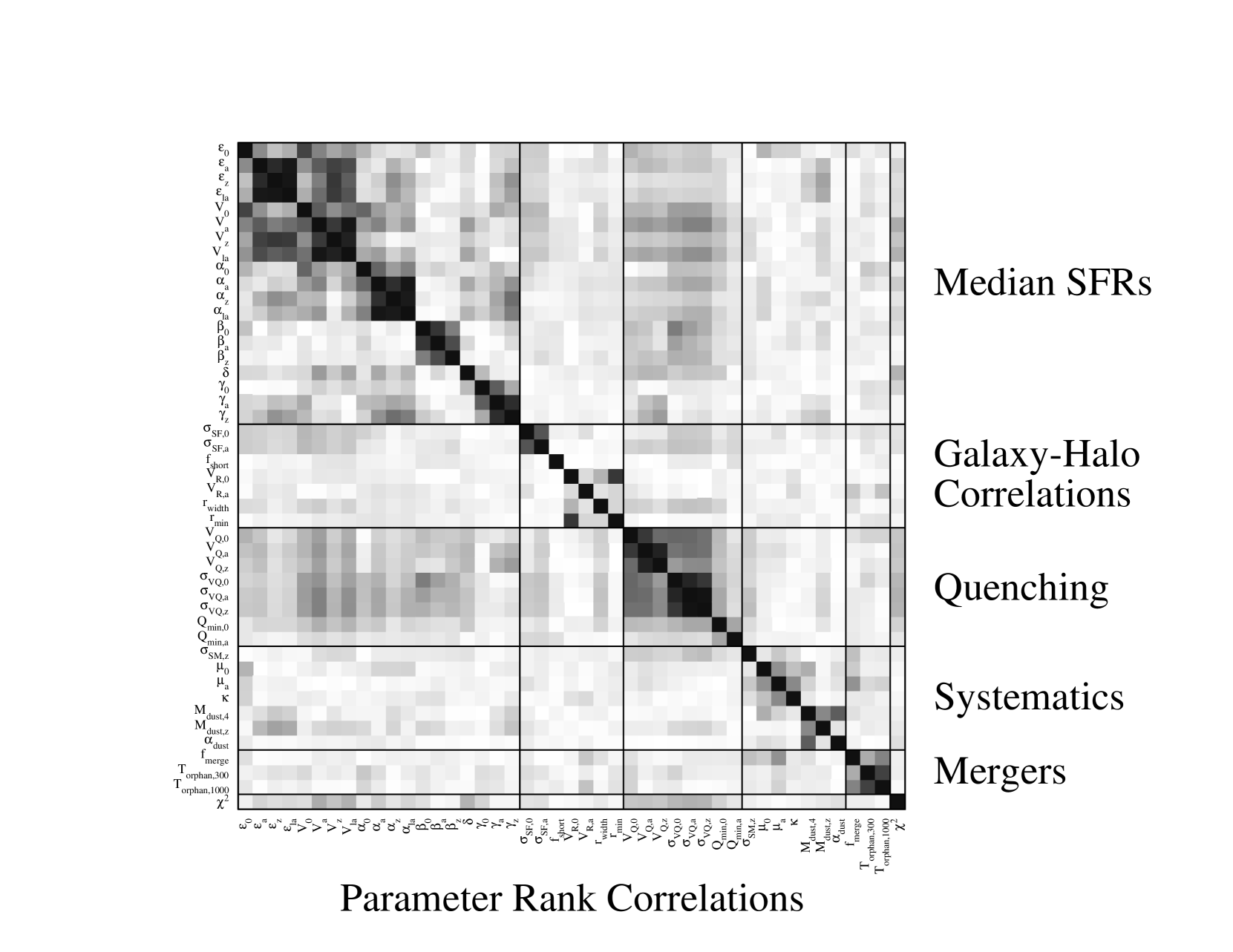
Figure I1: Rank correlations between parameters in the model posterior distribution. Darker shades indicate higher absolute values of rank correlation coefficients (both positive and negative). An interactive version of this figure that includes easy access to the underlying joint parameter distributions is available online.

Appendix I Parameter Correlations

Rank correlations between parameters in the model posterior distribution are shown in Fig. I1. Correlations between parameters that specify the redshift scaling are common and expected. For example, $\ln(1+z)$ scales similarly at $z<0.25$ to $1-a$ and to $z$, resulting in strong natural degeneracies between $\epsilon_{\mathrm{a}}$, $\epsilon_{\mathrm{la}}$, and $\epsilon_{\mathrm{z}}$. Note that this does not imply that an equally good fit could be obtained by removing two of these parameters—only that they are not orthogonal. In fact, the UniverseMachine internally uses linear combinations of parameters to increase orthogonality, reducing burn-in time. See Appendix E for an explanation of the chosen parameterization; the redshift scalings were chosen due to ease of interpretation and implementation, rather than orthogonality.

Several correlations are physically intuitive. Increasing both median SFRs and quenched fractions appropriately will leave predicted SMFs unchanged, leading to natural degeneracy between the parameter groups. Systematics parameters are degenerate with both median SFRs and quenched fractions for the same reason. Within the systematics parameters, $M_{\mathrm{dust}}$ correlates with $\mu_{0}$, suggesting that the UV luminosity function can be left unchanged by increasing both dust and the total stellar mass produced. Luminosity functions in redder bands are hence critical to break this type of degeneracy. Since the total intrahalo light is not being used as a constraint, the distance for satellites to merge into the intrahalo light is modestly degenerate with the threshold for keeping satellites as orphan galaxies.

Two non-correlations are also worth noting. Within median SFRs, the scaling for low-mass galaxies ($\alpha$) is independent of the scaling for high-mass galaxies ($\beta$). This is expected as the double power-law functional form for $SFR_{\mathrm{SF}}$ effectively isolates the two parameters, and predictions for the constraining data sets (total SMFs for $\alpha$ and high-mass SSFRs for $\beta$) can be adjusted relatively independently. In addition, parameters for the strength of the galaxy-halo assembly connection are relatively uncorrelated with median SFRs, as the former have little effect on the total stellar mass produced (which constrains median SFRs), and median SFRs have little effect on the separation in autocorrelation functions for quenched and star-forming galaxies (which constrains the galaxy-halo assembly correlation).

Appendix J Fits to Stellar Mass–Halo Mass Relations

To fit median stellar mass–halo mass relationships, we use:

$$\allowdisplaybreaks\log_{10}\left(\frac{M_{\ast}}{M_{1}}\right)= \,\epsilon-\log_{10}\left(10^{-\alpha x}+10^{-\beta x}\right)+\gamma\exp\left[-0.5\left(\frac{x}{\delta}\right)^{2}\right]$$ (62)

$$x\equiv \log_{10}\left(\frac{M_{\mathrm{peak}}}{M_{1}}\right)$$ (63)

This is a double power-law plus a Gaussian, similar to Eq. 7. The adopted redshift scaling is:

$$\log_{10}\left(\frac{M_{1}}{\;\mathrm{M}_{\odot}}\right)= \,M_{0}+M_{a}(a-1)-M_{\mathrm{lna}}\ln(a)+M_{z}z$$ (64)

$$\epsilon= \,\epsilon_{0}+\epsilon_{a}(a-1)-\epsilon_{\mathrm{lna}}\ln(a)+\epsilon_{z}z$$ (65)

$$\alpha= \,\alpha_{0}+\alpha_{a}(a-1)-\alpha_{\mathrm{lna}}\ln(a)+\alpha_{z}z$$ (66)

$$\beta= \,\beta_{0}+\beta_{a}(a-1)+\beta_{z}z$$ (67)

$$\delta= \,\delta_{0}$$ (68)

$$\log_{10}(\gamma)= \,\gamma_{0}+\gamma_{a}(a-1)+\gamma_{z}z$$ (69)

These formulae are fit to the mock catalogues’ actual median SM–HM relations at 22 redshifts ($z=0.1$ and $z=0-10$ in steps of $\Delta z=0.5$) in bins of width $0.2$ dex for $10^{10.5}\;\mathrm{M}_{\odot}<M_{\mathrm{peak}}<10^{15}\;\mathrm{M}_{\odot}$. Best-fitting parameters and uncertainties are shown in Table 10 for many different selection cuts. Fits were performed with a tolerance of 0.03 dex; $\chi^{2}$ values of $>200$ in Table 10 indicate that the fit often exceeded this tolerance. These cases only happen for quenched galaxies, when low-number statistics prevent good fits at high redshifts; nonetheless, if such fits are used, then comparison with the raw data accompanying this paper is necessary to ensure that the fits are not being used outside their well-fitting range.

The data in Table 10 and Python code to evaluate the fits at arbitrary redshifts are both available online.

Table 10: Fit Parameters for Stellar Mass–Halo Mass Relations

SM	Q/SF	Cen/Sat	IHL	$\epsilon_{0}$	$\epsilon_{a}$	$\epsilon_{\mathrm{lna}}$	$\epsilon_{z}$	$M_{0}$	$M_{a}$	$M_{\mathrm{lna}}$	$M_{z}$	$\alpha_{0}$	$\alpha_{a}$
				$\alpha_{\mathrm{lna}}$	$\alpha_{z}$	$\beta_{0}$	$\beta_{a}$	$\beta_{z}$	$\delta_{0}$	$\gamma_{0}$	$\gamma_{a}$	$\gamma_{z}$	$\chi^{2}$
Obs.	All	All	Excl.	$-1.435^{+0.023}_{-0.075}$	$1.831^{-0.066}_{-2.818}$	$1.368^{+0.089}_{-2.557}$	$-0.217^{+0.466}_{-0.048}$	$12.035^{+0.008}_{-0.100}$	$4.556^{+0.076}_{-2.453}$	$4.417^{+0.237}_{-2.255}$	$-0.731^{+0.464}_{-0.064}$	$1.963^{+0.163}_{-0.010}$	$-2.316^{+0.855}_{-1.361}$
				$-1.732^{+0.519}_{-1.271}$	$0.178^{+0.196}_{-0.084}$	$0.482^{+0.053}_{-0.002}$	$-0.841^{+0.709}_{+0.188}$	$-0.471^{+0.288}_{+0.049}$	$0.411^{+0.060}_{-0.087}$	$-1.034^{+0.264}_{-0.177}$	$-3.100^{+2.496}_{-0.363}$	$-1.055^{+0.973}_{-0.127}$	157
Obs.	All	Cen.	Excl.	$-1.435^{+0.015}_{-0.076}$	$1.813^{+0.044}_{-2.839}$	$1.353^{+0.242}_{-2.606}$	$-0.214^{+0.481}_{-0.075}$	$12.081^{+0.008}_{-0.080}$	$4.696^{+0.036}_{-2.398}$	$4.485^{+0.159}_{-2.237}$	$-0.740^{+0.446}_{-0.057}$	$1.957^{+0.137}_{-0.002}$	$-2.650^{+0.977}_{-1.406}$
				$-1.953^{+0.632}_{-1.310}$	$0.204^{+0.186}_{-0.116}$	$0.474^{+0.057}_{+0.000}$	$-0.903^{+0.746}_{+0.210}$	$-0.492^{+0.303}_{+0.062}$	$0.386^{+0.047}_{-0.068}$	$-1.065^{+0.266}_{-0.229}$	$-3.243^{+2.577}_{-0.346}$	$-1.107^{+1.010}_{-0.119}$	156
Obs.	All	Sat.	Excl.	$-1.449^{+0.102}_{-0.046}$	$-1.256^{+1.289}_{-0.377}$	$-1.031^{+1.076}_{-0.583}$	$0.108^{+0.156}_{-0.178}$	$11.896^{+0.033}_{-0.069}$	$3.284^{+0.427}_{-1.425}$	$3.413^{+0.513}_{-1.276}$	$-0.580^{+0.271}_{-0.098}$	$1.949^{+0.198}_{-0.022}$	$-4.096^{+1.604}_{+0.015}$
				$-3.226^{+1.204}_{-0.109}$	$0.401^{+0.043}_{-0.200}$	$0.477^{+0.016}_{-0.053}$	$0.046^{+0.150}_{-0.308}$	$-0.214^{+0.111}_{-0.157}$	$0.357^{+5.809}_{-0.060}$	$-0.755^{+0.027}_{-2.410}$	$0.461^{-0.084}_{-4.909}$	$0.025^{+0.062}_{-1.674}$	170
Obs.	Q	All	Excl.	$-1.471^{+0.027}_{-0.133}$	$-1.952^{+1.689}_{-0.153}$	$-2.508^{+1.920}_{-0.266}$	$0.499^{+0.094}_{-0.454}$	$12.021^{+0.062}_{-0.072}$	$3.368^{+0.129}_{-2.588}$	$3.615^{+0.164}_{-2.666}$	$-0.645^{+0.634}_{-0.018}$	$1.851^{+0.081}_{-0.211}$	$-4.244^{+4.170}_{+0.745}$
				$-4.402^{+4.680}_{+1.056}$	$0.803^{-0.258}_{-1.395}$	$0.505^{+0.058}_{-0.009}$	$-0.125^{+0.172}_{-0.159}$	$-0.094^{+0.097}_{-0.112}$	$0.461^{+0.069}_{-0.029}$	$-0.858^{+0.313}_{-0.099}$	$-0.933^{+0.492}_{-0.836}$	$-0.098^{+0.069}_{-0.198}$	184
Obs.	Q	Cen.	Excl.	$-1.480^{+0.028}_{-0.081}$	$-0.831^{+1.297}_{-0.731}$	$-1.351^{+1.433}_{-0.868}$	$0.321^{+0.225}_{-0.315}$	$12.069^{+0.032}_{-0.047}$	$2.646^{+0.466}_{-1.486}$	$2.710^{+0.599}_{-1.550}$	$-0.431^{+0.347}_{-0.159}$	$1.899^{+0.082}_{-0.090}$	$-2.901^{+2.210}_{-0.442}$
				$-2.413^{+2.492}_{-0.279}$	$0.332^{+0.035}_{-0.613}$	$0.502^{+0.047}_{-0.014}$	$-0.315^{+0.234}_{-0.132}$	$-0.218^{+0.134}_{-0.069}$	$0.397^{+0.067}_{-0.015}$	$-0.867^{+0.197}_{-0.110}$	$-1.146^{+0.432}_{-0.973}$	$-0.294^{+0.179}_{-0.349}$	202${\dagger}$
Obs.	SF	All	Excl.	$-1.441^{+0.037}_{-0.088}$	$1.697^{-0.186}_{-3.365}$	$1.326^{+0.041}_{-3.146}$	$-0.221^{+0.576}_{-0.052}$	$12.054^{+0.015}_{-0.095}$	$4.554^{-0.052}_{-2.725}$	$4.484^{+0.089}_{-2.536}$	$-0.750^{+0.522}_{-0.033}$	$1.976^{+0.146}_{-0.039}$	$-2.123^{+0.639}_{-1.519}$
				$-1.617^{+0.449}_{-1.328}$	$0.162^{+0.207}_{-0.091}$	$0.465^{+0.049}_{-0.023}$	$-1.071^{+1.051}_{+0.098}$	$-0.659^{+0.460}_{+0.000}$	$0.436^{+0.091}_{-0.108}$	$-1.016^{+0.240}_{-0.525}$	$-2.862^{+1.942}_{-0.897}$	$-0.941^{+0.800}_{-0.217}$	176
Obs.	SF	Cen.	Excl.	$-1.426^{+0.011}_{-0.116}$	$1.588^{+0.064}_{-3.211}$	$1.237^{+0.298}_{-3.066}$	$-0.210^{+0.539}_{-0.080}$	$12.071^{+0.025}_{-0.075}$	$4.633^{-0.048}_{-2.488}$	$4.527^{+0.050}_{-2.286}$	$-0.757^{+0.483}_{-0.030}$	$1.985^{+0.120}_{-0.053}$	$-2.492^{+0.820}_{-1.406}$
				$-1.860^{+0.609}_{-1.222}$	$0.188^{+0.196}_{-0.108}$	$0.448^{+0.067}_{-0.005}$	$-1.121^{+1.064}_{+0.111}$	$-0.665^{+0.442}_{+0.017}$	$0.407^{+0.113}_{-0.075}$	$-1.149^{+0.396}_{-0.295}$	$-3.221^{+2.266}_{-0.120}$	$-1.022^{+0.883}_{-0.038}$	178
True	All	All	Excl.	$-1.430^{+0.024}_{-0.143}$	$1.796^{-0.285}_{-2.992}$	$1.360^{-0.070}_{-2.830}$	$-0.216^{+0.495}_{-0.040}$	$12.040^{+0.004}_{-0.102}$	$4.675^{-0.003}_{-2.512}$	$4.513^{+0.154}_{-2.281}$	$-0.744^{+0.446}_{-0.054}$	$1.973^{+0.158}_{-0.016}$	$-2.353^{+0.748}_{-1.315}$
				$-1.783^{+0.466}_{-1.294}$	$0.186^{+0.191}_{-0.080}$	$0.473^{+0.065}_{+0.005}$	$-0.884^{+0.748}_{+0.249}$	$-0.486^{+0.300}_{+0.071}$	$0.407^{+0.079}_{-0.074}$	$-1.088^{+0.336}_{-0.170}$	$-3.241^{+2.649}_{+0.085}$	$-1.079^{+1.002}_{-0.053}$	115
True	All	All	Incl.	$-1.466^{+0.008}_{-0.177}$	$1.852^{+0.041}_{-2.940}$	$1.439^{+0.137}_{-2.853}$	$-0.227^{+0.493}_{-0.059}$	$12.013^{+0.015}_{-0.106}$	$4.597^{+0.084}_{-2.550}$	$4.470^{+0.257}_{-2.416}$	$-0.737^{+0.488}_{-0.069}$	$1.965^{+0.146}_{-0.053}$	$-2.137^{+0.763}_{-1.400}$
				$-1.607^{+0.572}_{-1.291}$	$0.161^{+0.215}_{-0.090}$	$0.564^{+0.091}_{+0.013}$	$-0.835^{+0.680}_{+0.115}$	$-0.478^{+0.293}_{+0.041}$	$0.411^{+0.082}_{-0.062}$	$-0.937^{+0.355}_{-0.077}$	$-2.810^{+2.417}_{+0.459}$	$-0.983^{+0.911}_{+0.135}$	130
True	All	Cen.	Excl.	$-1.431^{+0.024}_{-0.131}$	$1.757^{-0.146}_{-2.914}$	$1.350^{-0.021}_{-2.787}$	$-0.218^{+0.476}_{-0.049}$	$12.074^{+0.011}_{-0.083}$	$4.600^{+0.100}_{-2.297}$	$4.423^{+0.236}_{-2.179}$	$-0.732^{+0.429}_{-0.060}$	$1.974^{+0.136}_{-0.020}$	$-2.468^{+0.614}_{-1.448}$
				$-1.816^{+0.422}_{-1.388}$	$0.182^{+0.205}_{-0.077}$	$0.470^{+0.061}_{+0.004}$	$-0.875^{+0.744}_{+0.198}$	$-0.487^{+0.307}_{+0.066}$	$0.382^{+0.050}_{-0.067}$	$-1.160^{+0.363}_{-0.121}$	$-3.634^{+2.907}_{+0.154}$	$-1.219^{+1.132}_{+0.029}$	126
True	All	Cen.	Incl.	$-1.462^{+0.006}_{-0.180}$	$1.882^{-0.033}_{-2.995}$	$1.446^{+0.117}_{-2.765}$	$-0.224^{+0.480}_{-0.055}$	$12.055^{+0.003}_{-0.101}$	$4.667^{+0.101}_{-2.515}$	$4.471^{+0.254}_{-2.356}$	$-0.735^{+0.458}_{-0.067}$	$1.956^{+0.134}_{-0.037}$	$-2.570^{+0.941}_{-1.044}$
				$-1.904^{+0.678}_{-1.088}$	$0.198^{+0.169}_{-0.119}$	$0.558^{+0.093}_{+0.017}$	$-0.840^{+0.686}_{+0.128}$	$-0.472^{+0.287}_{+0.036}$	$0.393^{+0.046}_{-0.066}$	$-1.004^{+0.388}_{-0.016}$	$-2.983^{+2.514}_{+0.380}$	$-0.996^{+0.916}_{+0.079}$	142
True	All	Sat.	Excl.	$-1.432^{+0.083}_{-0.069}$	$-1.231^{+1.233}_{-0.415}$	$-0.999^{+0.969}_{-0.596}$	$0.100^{+0.127}_{-0.154}$	$11.889^{+0.041}_{-0.049}$	$3.236^{+0.131}_{-1.531}$	$3.378^{+0.264}_{-1.395}$	$-0.577^{+0.295}_{-0.050}$	$1.959^{+0.172}_{-0.022}$	$-4.033^{+1.786}_{-0.005}$
				$-3.175^{+1.391}_{-0.197}$	$0.390^{+0.056}_{-0.229}$	$0.464^{+0.019}_{-0.041}$	$0.130^{+0.248}_{-0.233}$	$-0.153^{+0.135}_{-0.133}$	$0.319^{+3.829}_{-0.060}$	$-0.812^{+0.079}_{-1.933}$	$0.522^{-0.047}_{-3.413}$	$0.064^{+0.031}_{-0.882}$	127
True	Q	All	Excl.	$-1.491^{+0.045}_{-0.145}$	$-2.313^{+1.835}_{-0.044}$	$-2.778^{+2.055}_{-0.370}$	$0.492^{+0.192}_{-0.438}$	$12.005^{+0.088}_{-0.057}$	$3.294^{+0.350}_{-2.069}$	$3.669^{+0.257}_{-2.309}$	$-0.683^{+0.603}_{-0.027}$	$1.852^{+0.070}_{-0.207}$	$-3.922^{+3.359}_{+0.432}$
				$-4.052^{+3.886}_{+0.636}$	$0.692^{-0.200}_{-1.087}$	$0.511^{+0.044}_{-0.024}$	$-0.028^{+0.092}_{-0.252}$	$-0.041^{+0.055}_{-0.160}$	$0.506^{+0.018}_{-0.076}$	$-0.858^{+0.276}_{-0.118}$	$-0.902^{+0.499}_{-0.897}$	$-0.041^{+0.033}_{-0.269}$	133
True	Q	Cen.	Excl.	$-1.462^{+0.022}_{-0.136}$	$-0.732^{+0.798}_{-1.226}$	$-1.273^{+0.970}_{-1.471}$	$0.302^{+0.296}_{-0.266}$	$12.072^{+0.042}_{-0.036}$	$3.581^{+0.000}_{-2.035}$	$3.665^{+0.109}_{-1.998}$	$-0.634^{+0.425}_{-0.056}$	$1.928^{+0.053}_{-0.126}$	$-3.472^{+1.880}_{-0.756}$
				$-3.119^{+2.116}_{-0.431}$	$0.507^{+0.009}_{-0.522}$	$0.488^{+0.047}_{-0.010}$	$-0.419^{+0.349}_{+0.016}$	$-0.256^{+0.226}_{-0.023}$	$0.406^{+0.083}_{-0.027}$	$-0.980^{+0.273}_{-0.090}$	$-1.443^{+0.695}_{-0.702}$	$-0.335^{+0.252}_{-0.231}$	153
True	SF	All	Excl.	$-1.494^{+0.083}_{-0.105}$	$1.569^{-0.202}_{-3.177}$	$1.293^{-0.010}_{-2.898}$	$-0.215^{+0.514}_{-0.027}$	$12.059^{-0.000}_{-0.106}$	$4.645^{-0.160}_{-2.402}$	$4.544^{+0.000}_{-2.244}$	$-0.757^{+0.446}_{-0.032}$	$1.905^{+0.216}_{+0.037}$	$-2.555^{+0.815}_{-1.204}$
				$-1.875^{+0.607}_{-1.180}$	$0.197^{+0.187}_{-0.110}$	$0.509^{+0.032}_{-0.053}$	$-0.889^{+1.073}_{+0.347}$	$-0.538^{+0.441}_{+0.103}$	$0.460^{+0.069}_{-0.125}$	$-0.807^{+0.093}_{-0.623}$	$-1.859^{+1.187}_{-0.659}$	$-0.637^{+0.526}_{-0.185}$	98
True	SF	Cen.	Excl.	$-1.459^{+0.040}_{-0.155}$	$1.515^{-0.058}_{-3.018}$	$1.249^{+0.104}_{-2.703}$	$-0.214^{+0.488}_{-0.048}$	$12.060^{+0.026}_{-0.074}$	$4.609^{-0.072}_{-2.215}$	$4.525^{+0.017}_{-2.098}$	$-0.756^{+0.423}_{-0.032}$	$1.972^{+0.142}_{-0.030}$	$-2.523^{+0.728}_{-1.469}$
				$-1.868^{+0.591}_{-1.382}$	$0.188^{+0.219}_{-0.097}$	$0.488^{+0.059}_{-0.044}$	$-0.965^{+1.083}_{+0.306}$	$-0.569^{+0.450}_{+0.106}$	$0.391^{+0.331}_{-0.059}$	$-0.958^{+0.260}_{-0.440}$	$-2.230^{+1.598}_{-0.282}$	$-0.706^{+0.588}_{-0.165}$	98

Notes. Python code to generate SMHM relations for all these fits at arbitrary redshifts is included in the UniverseMachine distribution online. Large numbers show the parameters for the best-fitting model, and uncertainties show the 68% confidence interval for the model posterior distribution. ${\dagger}$Fits with $\chi^{2}>200$ indicate features in the underlying raw data that are not well-captured. Direct comparison with the raw data included in the data release should be done to verify that the fit is not being used inappropriately.

References

- Abadi et al. (2010) Abadi M. G., Navarro J. F., Fardal M., Babul A., Steinmetz M., 2010, MNRAS, 407, 435
- Abazajian et al. (2009) Abazajian K. N., et al., 2009, ApJS , 182, 543
- Abramson et al. (2015) Abramson L. E., Gladders M. D., Dressler A., Oemler Jr. A., Poggianti B., Vulcani B., 2015, ApJL , 801, L12
- Abramson et al. (2016) Abramson L. E., Gladders M. D., Dressler A., Oemler Jr. A., Poggianti B., Vulcani B., 2016, ApJ , 832, 7
- Aihara et al. (2018) Aihara H., et al., 2018, PASJ, 70, S4
- An et al. (2014) An F. X., et al., 2014, ApJ , 784, 152
- Baldry et al. (2012) Baldry I. K., et al., 2012, MNRAS, 421, 621
- Balogh et al. (2016) Balogh M. L., et al., 2016, MNRAS, 456, 4364
- Bauer et al. (2013) Bauer A. E., et al., 2013, MNRAS, 434, 209
- Becker (2015) Becker M. R., 2015, preprint, (arXiv:1507.03605)
- Behroozi & Silk (2015) Behroozi P. S., Silk J., 2015, ApJ , 799, 32
- Behroozi & Silk (2018) Behroozi P., Silk J., 2018, MNRAS, 477, 5382
- Behroozi et al. (2010) Behroozi P. S., Conroy C., Wechsler R. H., 2010, ApJ , 717, 379
- Behroozi et al. (2013a) Behroozi P. S., Loeb A., Wechsler R. H., 2013a, JCAP, 6, 19
- Behroozi et al. (2013b) Behroozi P. S., Wechsler R. H., Wu H.-Y., 2013b, ApJ , 762, 109
- Behroozi et al. (2013c) Behroozi P. S., Wechsler R. H., Conroy C., 2013c, ApJL , 762, L31
- Behroozi et al. (2013d) Behroozi P. S., Wechsler R. H., Wu H.-Y., Busha M. T., Klypin A. A., Primack J. R., 2013d, ApJ , 763, 18
- Behroozi et al. (2013e) Behroozi P. S., Wechsler R. H., Conroy C., 2013e, ApJ , 770, 57
- Behroozi et al. (2013f) Behroozi P. S., Marchesini D., Wechsler R. H., Muzzin A., Papovich C., Stefanon M., 2013f, ApJL , 777, L10
- Behroozi et al. (2014a) Behroozi P. S., Wechsler R. H., Lu Y., Hahn O., Busha M. T., Klypin A., Primack J. R., 2014a, ApJ , 787, 156
- Behroozi et al. (2014b) Behroozi P. S., Ramirez-Ruiz E., Fryer C. L., 2014b, ApJ , 792, 123
- Behroozi et al. (2015a) Behroozi P. S., et al., 2015a, MNRAS, 450, 1546
- Behroozi et al. (2015b) Behroozi P., et al., 2015b, MNRAS, 454, 3020
- Behroozi et al. (2019) Behroozi P., et al., 2019, preprint, (arXiv:1903.04509)
- Bernardi et al. (2013) Bernardi M., Meert A., Sheth R. K., Vikram V., Huertas-Company M., Mei S., Shankar F., 2013, MNRAS, 436, 697
- Bernardi et al. (2016) Bernardi M., Meert A., Sheth R. K., Huertas-Company M., Maraston C., Shankar F., Vikram V., 2016, MNRAS, 455, 4122
- Bernardi et al. (2017) Bernardi M., Meert A., Sheth R. K., Fischer J.-L., Huertas-Company M., Maraston C., Shankar F., Vikram V., 2017, MNRAS, 467, 2217
- Berti et al. (2017) Berti A. M., Coil A. L., Behroozi P. S., Eisenstein D. J., Bray A. D., Cool R. J., Moustakas J., 2017, ApJ , 834, 87
- Béthermin et al. (2013) Béthermin M., Wang L., Doré O., Lagache G., Sargent M., Daddi E., Cousin M., Aussel H., 2013, A&A , 557, A66
- Béthermin et al. (2015) Béthermin M., et al., 2015, A&A , 573, A113
- Binney & Tremaine (2008) Binney J., Tremaine S., 2008, Galactic Dynamics: Second Edition. Princeton University Press
- Birrer et al. (2014) Birrer S., Lilly S., Amara A., Paranjape A., Refregier A., 2014, ApJ , 793, 12
- Blanton et al. (2005) Blanton M. R., et al., 2005, AJ , 129, 2562
- Bouché et al. (2010) Bouché N., et al., 2010, ApJ , 718, 1001
- Bouwens et al. (2014) Bouwens R. J., et al., 2014, ApJ , 793, 115
- Bouwens et al. (2015) Bouwens R. J., et al., 2015, ApJ , 803, 34
- Bouwens et al. (2016a) Bouwens R. J., et al., 2016a, ApJ , 830, 67
- Bouwens et al. (2016b) Bouwens R. J., et al., 2016b, ApJ , 833, 72
- Brammer et al. (2012) Brammer G. B., et al., 2012, ApJS , 200, 13
- Brinchmann et al. (2004) Brinchmann J., Charlot S., White S. D. M., Tremonti C., Kauffmann G., Heckman T., Brinkmann J., 2004, MNRAS, 351, 1151
- Bruzual & Charlot (2003) Bruzual G., Charlot S., 2003, MNRAS, 344, 1000
- Bryan & Norman (1998) Bryan G. L., Norman M. L., 1998, ApJ , 495, 80
- Byler et al. (2017) Byler N., Dalcanton J. J., Conroy C., Johnson B. D., 2017, ApJ , 840, 44
- Byrd & Valtonen (1990) Byrd G., Valtonen M., 1990, ApJ , 350, 89
- Calzetti (2001) Calzetti D., 2001, New Astronomy Review, 45, 601
- Calzetti et al. (2000) Calzetti D., Armus L., Bohlin R. C., Kinney A. L., Koornneef J., Storchi-Bergmann T., 2000, ApJ , 533, 682
- Campbell et al. (2018) Campbell D., van den Bosch F. C., Padmanabhan N., Mao Y.-Y., Zentner A. R., Lange J. U., Jiang F., Villarreal A., 2018, MNRAS, 477, 359
- Chabrier (2003) Chabrier G., 2003, PASP , 115, 763
- Charlot & Fall (2000) Charlot S., Fall S. M., 2000, ApJ , 539, 718
- Chua et al. (2017) Chua K. T. E., Pillepich A., Rodriguez-Gomez V., Vogelsberger M., Bird S., Hernquist L., 2017, MNRAS, 472, 4343
- Clauwens et al. (2016) Clauwens B., Franx M., Schaye J., 2016, MNRAS, 463, L1
- Cohn (2017) Cohn J. D., 2017, MNRAS, 466, 2718
- Coil et al. (2011) Coil A. L., et al., 2011, ApJ , 741, 8
- Coil et al. (2017) Coil A. L., Mendez A. J., Eisenstein D. J., Moustakas J., 2017, ApJ , 838, 87
- Conroy (2013) Conroy C., 2013, ARAA , 51, 393
- Conroy & Gunn (2010) Conroy C., Gunn J. E., 2010, ApJ , 712, 833
- Conroy & Wechsler (2009) Conroy C., Wechsler R. H., 2009, ApJ , 696, 620
- Conroy & van Dokkum (2012) Conroy C., van Dokkum P. G., 2012, ApJ , 760, 71
- Conroy et al. (2009) Conroy C., Gunn J. E., White M., 2009, ApJ , 699, 486
- Conroy et al. (2013) Conroy C., Dutton A. A., Graves G. J., Mendel J. T., van Dokkum P. G., 2013, ApJL , 776, L26
- Coupon et al. (2015) Coupon J., et al., 2015, MNRAS, 449, 1352
- Cowley et al. (2018) Cowley W. I., et al., 2018, ApJ , 853, 69
- Croton & Farrar (2008) Croton D. J., Farrar G. R., 2008, MNRAS, 386, 2285
- Croton et al. (2016) Croton D. J., et al., 2016, ApJS , 222, 22
- Cucciati et al. (2012) Cucciati O., et al., 2012, A&A , 539, A31
- D’Souza et al. (2015) D’Souza R., Vegetti S., Kauffmann G., 2015, MNRAS, 454, 4027
- Davé et al. (2010) Davé R., Finlator K., Oppenheimer B. D., Fardal M., Katz N., Kereš D., Weinberg D. H., 2010, MNRAS, 404, 1355
- Davé et al. (2016) Davé R., Thompson R., Hopkins P. F., 2016, MNRAS, 462, 3265
- Davies et al. (2015) Davies L. J. M., et al., 2015, MNRAS, 447, 1014
- De Rijcke et al. (2013) De Rijcke S., Schroyen J., Vandenbroucke B., Jachowicz N., Decroos J., Cloet-Osselaer A., Koleva M., 2013, MNRAS, 433, 3005
- Dekel & Birnboim (2006) Dekel A., Birnboim Y., 2006, MNRAS, 368, 2
- Dickey et al. (2016) Dickey C. M., et al., 2016, ApJL , 828, L11
- Diemer & Kravtsov (2015) Diemer B., Kravtsov A. V., 2015, ApJ , 799, 108
- Diemer et al. (2013) Diemer B., More S., Kravtsov A. V., 2013, ApJ , 766, 25
- Dodelson & Schneider (2013) Dodelson S., Schneider M. D., 2013, Phys. Rev. D, 88, 063537
- Dolag et al. (2016) Dolag K., Komatsu E., Sunyaev R., 2016, MNRAS, 463, 1797
- Drake et al. (2013) Drake A. B., et al., 2013, MNRAS, 433, 796
- Drake et al. (2015) Drake A. B., et al., 2015, MNRAS, 454, 2015
- Dressler & Gunn (1983) Dressler A., Gunn J. E., 1983, ApJ , 270, 7
- Dubois et al. (2016) Dubois Y., Peirani S., Pichon C., Devriendt J., Gavazzi R., Welker C., Volonteri M., 2016, MNRAS, 463, 3948
- Duncan et al. (2014) Duncan K., et al., 2014, MNRAS, 444, 2960
- Dunne et al. (2009) Dunne L., et al., 2009, MNRAS, 394, 3
- Emerick et al. (2016) Emerick A., Mac Low M.-M., Grcevich J., Gatto A., 2016, ApJ , 826, 148
- Fakhouri et al. (2010) Fakhouri O., Ma C.-P., Boylan-Kolchin M., 2010, MNRAS, 406, 2267
- Fang et al. (2018) Fang J. J., et al., 2018, ApJ , 858, 100
- Farouki & Shapiro (1981) Farouki R., Shapiro S. L., 1981, ApJ , 243, 32
- Fillingham et al. (2018) Fillingham S. P., Cooper M. C., Boylan-Kolchin M., Bullock J. S., Garrison-Kimmel S., Wheeler C., 2018, MNRAS, 477, 4491