Force-dependent unbinding rate of molecular motors
from stationary optical trap data

Abstract

Molecular motors walk along filaments until they detach stochastically with a force-dependent unbinding rate. Here, we show that this unbinding rate can be obtained from the analysis of experimental data of molecular motors moving in stationary optical traps. Two complementary methods are presented, based on the analysis of the distribution for the unbinding forces and of the motor’s force traces. In the first method, analytically derived force distributions for slip bonds, slip-ideal bonds, and catch bonds are used to fit the cumulative distributions of the unbinding forces. The second method is based on the statistical analysis of the observed force traces. We validate both methods with stochastic simulations and apply them to experimental data for kinesin-1.

Introduction.

In mammals, at least 80 genes code for different cytoskeletal motors that transduce chemical free energy into mechanical work Howard (2005); Schliwa and Woehlke (2003). These molecular motors perform nanometer steps along filaments from which they unbind stochastically after a finite run length Lipowsky and Klumpp (2005). Both their stepping dynamics and their unbinding behavior are strongly affected by external forces. In cells, these forces arise, e.g., from viscous drag, from the elastic coupling to other force-producing molecules, or from their cargo load Hunt et al. (1994); Rogers et al. (2009); Coppin et al. (1997). Thus, stepping and unbinding are characterized by a force-velocity relation and a force-dependent unbinding rate, respectively.

Our understanding of how different molecular motors respond to external forces is primarily based on single-motor experiments with optical traps Veigel and Schmidt (2011). Whereas the force-velocity relations have been studied for a variety of motors Coppin et al. (1997); Carter and Cross (2005); Schnitzer et al. (2000); Clemen et al. (2005); Gennerich et al. (2007), the force-dependent unbinding rate has been elucidated only for the kinesin-1 motor Andreasson et al. (2015); Coppin et al. (1997); Thorn et al. (2000). The motor-filament bond of kinesin behaves as a slip bond, i.e., the unbinding probability increases with increasing load force. In contrast, the dynein motor may exhibit catch bond behavior, i.e., may bind to the filament more strongly under force Andreasson et al. (2015); Rai et al. (2013). Furthermore, single dynein heads behave as slip-ideal bonds, i.e., the unbinding rate first increases with force and then becomes essentially force-independent Nicholas et al. (2015). Developing reliable methods to determine the force-dependent unbinding behavior of molecular motors, is important to advance our understanding of their functions.

In a standard setup, a single molecular motor pulls a bead against the resisting force of a stationary optical trap Coppin et al. (1997). While the motor moves away from the center of the trap, the force on the bead increases until the motor unbinds from the filament and the bead snaps back to the trap center, see Fig. 1. The force at which the motor unbinds defines the unbinding force and a distribution of these forces can be constructed from many such events.

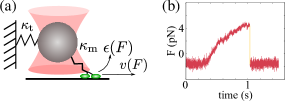
Figure 1: (color online). Molecular motor in a stationary optical trap (a) As the motor pulls the bead out of the trap center with velocity $v(F)$, the force $F$ on the motor increases, slows the motor down until it unbinds from the filament, and the bead falls back to the trap center. The stochastic unbinding is governed by the force-dependent unbinding rate $\epsilon(F)$. (b) The shape of the force trace depends on the motor dynamics and on the stiffnesses $\kappa_{\rm{t}}$ and $\kappa_{\rm{m}}$ of trap and motor. The unbinding rate $\epsilon(F)$ is an independent motor parameter that reflects the molecular interactions between motor and filament.

In the present letter, we derive analytical expressions for the unbinding force distributions. Comparing these results to experimental data allows us to identify the underlying filament-motor bond behavior. Furthermore, we estimate the force-dependent unbinding rate with a complementary approach based on the statistical analysis of force traces Coppin et al. (1997); Thorn et al. (2000). The latter method uses the information of the whole trace and does not require prior knowledge of the motor’s elastic properties or of its force-velocity relation. We explicitly show how both methods are connected and discuss their limitations. After validating both methods with stochastic simulations, we apply them to experimental data to determine the force-dependent unbinding behavior of kinesin-1.

Distribution-based method.

The first method is based on the distribution $p(F)$ of the unbinding forces as measured experimentally or in simulations. To derive analytical expressions for the distribution, we extend a method previously used to analyze force-spectroscopic data of single molecules Dudko et al. (2006, 2008). This method transforms the distribution of unbinding forces into the force-dependent unbinding rate

$$\epsilon(F)=\frac{\dot{F}(F)\,p(F)}{1-\int_{0}^{F}p(F^{\prime})dF^{\prime}},$$ (1)

in which $\dot{F}(F)$ is the force-dependent loading rate, i.e., the rate at which the force changes. From (1), we obtain the probability distribution function (pdf)

$$p(F)=\frac{\epsilon(F)}{\dot{F}(F)}\exp\left[-\int_{0}^{F}\frac{\epsilon(F^{\prime})}{\dot{F}(F^{\prime})}dF^{\prime}\right]$$ (2)

for the unbinding force. The latter equation implies that the distribution $p(F)$ is determined by the ratio of unbinding rate $\epsilon(F)$ to loading rate $\dot{F}(F)$. Therefore, from the pdfs for the unbinding force, we can only estimate the ratio $\epsilon/\dot{F}$, but not the unbinding rate alone without knowing the loading rate.

However, we can estimate $\dot{F}$ from a theoretical description of the motor. In the simplest case, the motor has a linear force-velocity relation $v(F)\equiv v_{0}(1-F/F_{\rm{s}})$, in which $F_{\rm{s}}$ is the stall force and $v_{0}$ the load-free velocity Klumpp et al. (2015). The force-extension relation of the motor molecule is assumed to be linear with spring constant $\kappa_{\rm{m}}$. This spring is connected in series with the spring-like potential of the optical trap described by the spring constant $\kappa_{\rm{t}}$. Using this motor description, we obtain the force-dependent loading rate $\dot{F}(F)=\kappa_{\rm{eff}}v_{0}(1-F/F_{\rm{s}})$ with the effective stiffness $\kappa_{\rm{eff}}\equiv\kappa_{\rm{m}}\kappa_{\rm{t}}/(\kappa_{\rm{m}}+\kappa_{\rm{t}})$. First, we assume that the motor exhibits slip-bond behavior with unbinding rate $\epsilon(F)\equiv\epsilon_{0}\exp(F/F_{\rm{d}})$, the detachment force $F_{\rm{d}}$ and the load-free unbinding rate $\epsilon_{0}$. For such an unbinding rate, the relation (2) leads to the unbinding force distribution

$$p(F)=\frac{F_{\rm{s}}\epsilon_{0}e^{F/F_{\rm{d}}}}{\kappa_{\rm{eff}}v_{0}(F_{\rm{s}}-F)}\exp\left[-\frac{F_{\rm{s}}\epsilon_{0}}{\kappa_{\rm{eff}}v_{0}}\Phi(F)\right]$$ (3)

with

$$\Phi(F)\equiv e^{F_{\rm{s}}/F_{\rm{d}}}\left(I\left(\frac{F_{\rm{s}}-F}{F_{\rm{d}}}\right)-I\left(\frac{F_{\rm{s}}}{F_{\rm{d}}}\right)\right)$$ (4)

and the exponential integral function $I(x)\equiv\int_{x}^{\infty}t^{-1}\exp[-t]dt$. In a similar way, we calculate exact expressions for the distribution of unbinding forces for slip-ideal and catch bonds Berger (2020). These expressions can be used to fit empirical cumulative distributions constructed from data, thereby estimating the unbinding rate $\epsilon(F)$. To validate our distribution-based approach, we use stochastic simulations to generate data sets of unbinding forces for different types of motor-filament bonds Berger (2020).

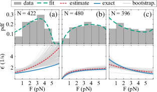
Figure 2: (color online). Distribution-based estimate of the unbinding rate (simulation study) From a stochastic simulation of a molecular motor in an optical trap, we obtain a set of unbinding forces from which we construct an empirical cumulative distribution function Berger (2020). We fit these cumulative distributions by the cumulative distributions as obtained from the analytically derived unbinding-force distributions (or pdfs) $p(F)$. Optimizing these fits, we obtain the distributions displayed as green lines, which are in good agreement with the gray normalized histograms for (a) slip bonds, (b) slip-ideal bonds, and (c) catch bonds. The corresponding unbinding rate $\epsilon(F)$ are the red lines in the lower panels. For comparison, we also display the unbinding rates used to generate the data (blue lines). The gray lines in the lower panels illustrate the variability of the unbinding rate from bootstrapping Berger (2020).

To account for the experimental noise in the trajectories, we add an appropriate level of noise to the simulated data. In this way, we generate three different data sets for slip, slip-ideal, and catch bonds. We choose the parameter values for the three different bonds such that the resulting unbinding rates have a comparable numerical range, see Fig. 2. We then use the analytically derived expressions for the unbinding-force distributions to fit the empirical cumulative distributions of the simulated data to deduce the parameters of the unbinding rates. The three different force-dependent unbinding behaviors lead to distinct unbinding-force distributions, see green lines in Fig. 2. The estimated parameters are in good agreement with the parameters used to generate the data Berger (2020). However, this agreement reflects, to a large extend, our knowledge about the assumed functional forms of the unbinding rates and of the dynamics of the motor. Next, we describe a method that uses the whole ensemble of force traces to estimate the unbinding rate without assuming any microscopic model.

Trace-based method.

To estimate the force-dependent unbinding rate from experimental data, without any assumptions about the motor-filament bonds and the force-velocity relation, it is necessary to estimate both the loading rate $\dot{F}$ and the distribution $p(F)$ of unbinding forces, see Eq. 1. The loading rate $\dot{F}$ can be estimated from the slope of the force traces before unbinding and $p(F)$ can be obtained as a histogram of the unbinding forces Dudko et al. (2008). The histogram has $N$ bins with bin width $\Delta F$. The height $h_{i}$ of the $i$-th bin is determined from the counts $C_{i}$ per bin as $h_{i}=C_{i}/(N^{\rm{un}}\Delta F)$ with $N^{\rm{un}}\equiv\sum_{i}C_{i}$. An estimator for the force-dependent unbinding rate in (1) is then given by Dudko et al. (2008)

$$\epsilon[(k-\textstyle{\frac{1}{2}}\displaystyle)\Delta F]=\frac{\dot{F}[(k-\frac{1}{2})\Delta F]h_{k}}{\Delta F(\frac{h_{k}}{2}+\sum_{i=k+1}^{N}h_{i})}.$$ (5)

This equation involves the force-dependent loading rate $\dot{F}[(k-\frac{1}{2})\Delta F]$ which has to be determined from the slopes of the force traces. We rewrite (5) in such a way that the unbinding rate can be estimated directly from the data points of the force traces Berger (2020). We bin the data points of all force traces into $N$ force bins with bin width $\Delta F$ and label $k$. We determine the numbers $C^{\rm{un}}_{k}$ of unbinding events and the number $C^{\rm{to}}_{k}$ of data points of all force traces per bin. The force-dependent unbinding rate is then given by

$$\epsilon[(k-\textstyle{\frac{1}{2}}\displaystyle)\Delta F]=\frac{C^{\rm{un}}_{k}}{\delta t\,C^{\rm{to}}_{k}},$$ (6)

in which $\delta t$ is the time step between the recorded points of the trace. Thus $\delta t\,C^{\rm{to}}_{k}$ represents the total time of all force traces spent in the $k$-th bin. To evaluate this equation neither a microscopic model nor any kind of fitting procedure is needed. Applying this approach to our simulated data, we determine the underlying force-dependent unbinding rate solely from the force traces, see Fig. 3. Even though the distributions of the unbinding forces for the slip-ideal and the catch bond appear to be similar, see Fig. 2, the trace-based method distinguishes the different unbinding behaviors remarkably well.

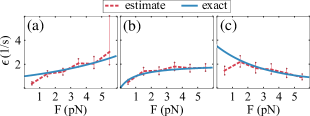
Figure 3: (color online). Trace-based estimate of the unbinding rate (simulation study) Without assuming a microscopic model, we only use the unbinding forces and the force traces from the stochastic simulations to estimate the unbinding rate for the three bond behaviors: slip bond (a), slip-ideal bond (b), and catch bond (c). The estimated unbinding rates (red lines) are in very good agreement with the exact unbinding rates used for the simulations (blue lines). The 95% confidence intervals are obtained from bootstrapping Berger (2020).

The unbinding rate of kinesin-1.

We apply both methods to experimental data of kinesin-1 pulling a bead out of a stationary optical trap. The data was obtained during control experiments carried out for a previous study DeBerg et al. (2013). The force-free velocity $v_{0}\simeq 484\,\rm{nm}/\rm{s}$ and the trap stiffness $\kappa_{\rm{t}}\simeq 0.03\,\rm{pN}/\rm{nm}$ DeBerg et al. (2013). We assume a motor stiffness of $\kappa_{\rm{m}}\simeq 0.3\,\rm{pN}/\rm{nm}$ Coppin et al. (1997). However, this assumption is not crucial because the effective stiffness $\kappa_{\rm{eff}}$ is dominated by the much smaller trap stiffness $\kappa_{\rm{t}}$. We determine the unbinding rate from a fit of the empirical cumulative distribution function constructed from 682 unbinding events, see Fig. 4(a,b) and Berger (2020). Despite our simplifying assumptions, the fit is in good agreement with the data, indicating that kinesin’s unbinding rate is consistent with a slip-bond behavior. We find the following optimal parameters with confidence intervals given in brackets: $\epsilon_{0}\simeq 0.97\,[0.80;1.35]\,\rm{s}^{-1}$, $F_{\rm{d}}\simeq 2.25\,[2.03;5.18]\,\rm{pN}$, and $F_{\rm{s}}\simeq 14.97\,[6.26;15]\,\rm{pN}$. Using the trace-based approach, we determine the force-dependent unbinding rate of kinesin-1 from Eq. S19 as shown in Fig. 4(d). An exponential fit excluding the boundary points leads to a detachment force of $F_{\rm{d}}\simeq 7.4\,\rm{pN}$ and a force-free unbinding rate of $\epsilon_{0}\simeq 1.1\,\rm{s}^{-1}$.

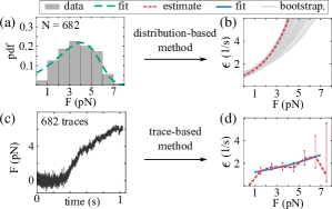
Figure 4: (color online). Unbinding rate of kinesin-1 (experimental data) (a,b) Distribution-based method: We use the analytical expression in Eq. 3 for a slip bond to fit the empirical cumulative distribution constructed from the experimental data Berger (2020). The numerical values of the fitted parameters determine the unbinding-force pdf $p(F)$ (green line in panel a) and the unbinding rate $\epsilon(F)$ (red line in panel b). For comparison, the distribution of the experimental data is estimated by a gray histogram. (c,d) Trace-based method: We use all 682 force traces —one example shown in (c) —to obtain the unbinding rate $\epsilon(F)$ as the red line in (d) from Eq. S19. Fitting this trace-based estimate with an exponential function (blue line), we obtain the force-free unbinding rate $\epsilon_{0}\simeq 1.1\,\rm{s}^{-1}$ and the detachment force $F_{\rm{d}}\simeq 7.4\,\rm{pN}$. In (b), the gray lines illustrate the variability of the unbinding rate from bootstrapping; in (d) the errors are given as 95% confidence intervals Berger (2020).

Discussion.

We have explicitly derived the distribution of unbinding forces of a single molecular motor in a stationary optical trap and validated it by stochastic simulations. The trace-based method reliably infers the correct unbinding behavior from the simulated data, see Fig. 3.

Furthermore, we have shown that a simple description of kinesin-1 is consistent with the experimental distribution of unbinding forces. However, the consistency implies a smaller detachment force compared to the estimate obtained from the trace-based approach. In conclusion, our trace-based analysis suggests a force-free unbinding rate of $\epsilon_{0}\simeq 1.1\,\rm{s}^{-1}$ and a detachment force of $F_{\rm{d}}\simeq 7.5\,\rm{pN}$. While the unbinding rate is consistent with the value of $\epsilon_{0}\simeq 1.0\,\rm{s}^{-1}$ commonly used for kinesin-1, the detachment force is 2.5 times larger than the value of $F_{\rm{d}}\simeq 3\,\rm{pN}$ used in most theoretical studies Klumpp et al. (2015). However, recent experimental and modeling studies indicate a higher value of about $6-7\,\rm{pN}$ or even a more complicated behavior Andreasson et al. (2015); Arpağ et al. (2014); Sumi (2017).

Force-dependent unbinding has important consequences for the function of the motors in their cellular environment Chaudhary et al. (2018); Blehm et al. (2013); Berger et al. (2011). Theoretical descriptions based on single-molecule dynamics indicate that many emerging phenomena, such as cooperative transport and macroscopic force production can only be explained with a suitable force-dependent unbinding rate for the single motors Berger et al. (2012); Klumpp and Lipowsky (2005); Müller et al. (2008); Berger and Hudspeth (2017).

Our framework provides a systematic way to study the force-dependent unbinding rate of molecular motors and can be extended to describe more complex optical trapping experiments. To determine the unbinding rate for forces that exceed the stall force, the stage could be moved relative to the trap which adds only an extra term to the loading rate Nicholas et al. (2015).

A first step towards understanding the function of motor proteins is to determine biophysical quantities that are directly accessible to experiments Ruhnow et al. (2017). While the probability distribution of unbinding forces depends on the stiffness of the trap and also on the stiffness of the linker that connects the motor to the bead, the force-dependent unbinding rate is a characteristic property of the motor-filament bond. Therefore, our computational approach provides a systematic framework for future studies to distinguish different motor-filament bonds such as dynein’s catch bond from kinesin’s slip bond.

Acknowledgment.

We thank Paul Selvin, Hannah A. DeBerg and Benjamin H. Blehm for providing the experimental data and stimulating discussions. The experimental data was acquired under the support of the NIH. FB was supported by a grant from the Alexander von Humboldt-Foundation.

I Distribution of unbinding forces

For our distribution-based analysis we derive analytic expressions for the distribution of unbinding forces for three different force-dependent bond behaviors.

I.1 The slip bond

We describe a slip bond with an unbinding rate that increases with the external force as

$$\epsilon(F)\equiv\epsilon_{0}\exp(F/F_{\rm{d}}).$$ (S1)

Here, we introduce the force-free unbinding rate $\epsilon_{0}$ and the characteristic detachment force $F_{\rm{d}}$. To calculate the corresponding distribution of unbinding forces, we proceed as explained in the main text and find

$$p(F)=\frac{F_{\rm{s}}\epsilon_{0}\exp[F/F_{\rm{d}}]}{\kappa_{\rm{eff}}v_{0}(F_{\rm{s}}-F)}\exp\left[-\frac{\epsilon_{0}\exp[F_{\rm{s}}/F_{\rm{d}}]F_{\rm{s}}}{\kappa_{\rm{eff}}v_{0}}\left(I\left(\frac{F_{\rm{s}}-F}{F_{\rm{d}}}\right)-I\left(\frac{F_{\rm{s}}}{F_{\rm{d}}}\right)\right)\right],$$ (S2)

with the exponential integral function

$$I(x)\equiv\int_{x}^{\infty}t^{-1}\exp[-t]dt.$$ (S3)

This equation implies that we cannot obtain $v_{0}$, $\kappa_{\rm{eff}}$ and $\epsilon_{0}$ independently from a fit, only the combination

$$F_{\rm{c}}\equiv\frac{v_{0}\kappa_{\rm{eff}}}{\epsilon_{0}}$$ (S4)

that defines the characteristic force $F_{\rm{c}}$. We simplify the distribution to

$$p(F|F_{\rm{c}},F_{\rm{d}},F_{\rm{s}})=\frac{F_{\rm{s}}\exp[F/F_{\rm{d}}]}{F_{\rm{c}}(F_{\rm{s}}-F)}\exp\left[-(F_{\rm{s}}/F_{\rm{c}})\exp[F_{\rm{s}}/F_{\rm{d}}]\left(I\left(\frac{F_{\rm{s}}-F}{F_{\rm{d}}}\right)-I\left(\frac{F_{\rm{s}}}{F_{\rm{d}}}\right)\right)\right],$$ (S5)

which depends now on the three parameters, $F_{\rm{c}}$, $F_{\rm{d}}$, and $F_{\rm{s}}$.

I.2 The slip-ideal bond

An ideal bond is characterized by a constant unbinding rate that is independent of the force dembo1994s ; nicholas2015s . As a phenomenological description for a slip-ideal bond with an unbinding rate that first increases with force and then becomes constant, we use the rational function

$$\epsilon(F)\equiv\frac{\epsilon_{0}F}{F_{\rm{a}}+F}.$$ (S6)

The corresponding probability distribution for the unbinding forces follows as

$$p(F|F_{\rm{a}},F_{\rm{c}},F_{\rm{s}})=\frac{FF_{\rm{s}}}{F_{\rm{c}}(F_{\rm{a}}+F)(F_{\rm{s}}-F)}\exp\left(\frac{F_{\rm{s}}}{F_{\rm{c}}(F_{\rm{a}}+F_{\rm{s}})}\left(F_{\rm{a}}\ln\left(1+\frac{F}{F_{\rm{a}}}\right)+F_{\rm{s}}\ln\left(1-\frac{F}{F_{\rm{s}}}\right)\right)\right),$$ (S7)

in which $F_{\rm{c}}$ is the characteristic force given in Eq. S4.

I.3 The catch bond

A catch bond is characterized by an unbinding rate that decreases with increasing force dembo1994s . We describe such a bond with the force-dependent unbinding rate

$$\epsilon(F)=\epsilon_{0}\exp(-F/F_{\rm{d}})+a.$$ (S8)

The corresponding distribution of unbinding forces reads

$$p(F|F_{\rm{a}},F_{\rm{c}},F_{\rm{d}},F_{\rm{s}}) =$$ (S9)

$$\frac{F_{\rm{s}}(F_{\rm{c}}/F_{\rm{a}}+\exp[-F/F_{\rm{d}}])}{F_{\rm{c}}(F_{\rm{s}}-F)}\exp\biggl{[}(F_{\rm{s}}/F_{\rm{c}})\exp[-F_{\rm{s}}/F_{\rm{d}}]\left(I\left(-\frac{F_{\rm{s}}}{F_{\rm{d}}}\right)-I\left(\frac{F-F_{\rm{s}}}{F_{\rm{d}}}\right)\right)+$$

$$(F_{\rm{s}}/F_{\rm{a}})(\ln(1-F/F_{\rm{s}})\biggr{)}\biggr{]},$$

in which $F_{\rm{c}}$ is defined in Eq. S4 and $F_{\rm{a}}\equiv v_{0}\kappa_{\rm{eff}}/a$.

II Simulations

To generate data for the validation of our methods, we assume that the motor steps forward with $\ell=8\,\rm{nm}$ steps with a force-dependent stepping rate $\alpha(F)$. We relate the stepping rate

$$\alpha(F)=v(F)/\ell=v_{0}(1-F/F_{\rm{s}})/\ell$$ (S10)

to a linear force velocity $v(F)$ described by the stall force $F_{\rm{s}}\simeq 6\,\rm{pN}$ and a typical force-free velocity $v_{0}\simeq 1\,\mu\rm{m/s}$. For studying the different unbinding behaviors we use the corresponding unbinding rates $\epsilon(F)$ introduced above and listed in Table 1. The stepping and unbinding of the motor are force-dependent and the force on the motor changes as it pulls the bead out of the center of the optical trap. To determine the force exerted on the motor, we assume a linear restoring force of the optical trap, characterized by a typical trap stiffness of $\kappa_{\rm{t}}\simeq 0.01\,\rm{pN}/\rm{nm}$ and a linear force-extension relation for the motor molecule with spring constant $\kappa_{\rm{m}}\simeq 0.3\,\rm{pN}/\rm{nm}$ coppin1997s . The force

$$F=\kappa_{\rm{t}}x_{\rm{b}}$$ (S11)

on the bead is determined from the distance $x_{\rm{b}}$ of the bead to the center of the trap. This distance changes with the position $x_{\rm{m}}$ of the motor, while it is moving out of the center of the trap, as

$$x_{\rm{b}}=\frac{\kappa_{\rm{m}}}{\kappa_{\rm{m}}+\kappa_{\rm{t}}}x_{\rm{m}}.$$ (S12)

Under the assumption that after each step the system reaches mechanical equilibrium instantaneously, the force on the bead equals the force on the bond of the motor and the filament with the corresponding loading rate

$$\dot{F}=\kappa_{\rm{t}}\frac{\kappa_{\rm{m}}}{\kappa_{\rm{m}}+\kappa_{\rm{t}}}\dot{x}_{\rm{m}}.$$ (S13)

We base our stochastic simulation on a Gillespie algorithm: at each step we calculate the force acting on the motor, adjust the stepping and unbinding rates accordingly and choose the next event with the corresponding probability gillespie1977s . If the motor steps forward, we increase the position $x_{\rm{m}}$ by the step size $\ell$. If the motor unbinds from the filament, we set the position to $x_{\rm{m}}=0$. In this way, we obtain trajectories of a single molecular motor as it pulls the bead out of a stationary trap. We convert the spatial trajectories corresponding to the bead position as a function of time into forces traces by multiplying the bead position with the stiffness of the trap. To mimic the experimental force traces as closely as possible, we add Gaussian white noise with a standard deviation of $\sigma=0.3\,\rm{pN}$, as estimated from the experimental data. An example of such a force trace is shown in Fig. S1(a).

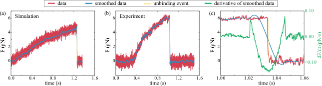
Figure S1: Analysis of force traces The original data (red) from the simulations and experiments are smoothed with a Savitzky-Golay filter (blue) and one example for each are shown in (a) and (b) respectively. Our unbinding detection algorithm determines the magnitude of the unbinding force (yellow) and displays it close to the unbinding event to allow for visual inspection. To explain the basic idea of the algorithm, we magnified the unbinding event of (b) in (c) and show the derivative as the discrete difference (green) between points of the smoothed force trace. The location of the two maxima of the derivative are reliable estimates of time points before and after the unbinding event. Taking the difference of the averages of the traces before and after the unbinding event provides the numerical value for the unbinding force.

III Detection of unbinding forces from the force traces

The experiments and the simulations provide long force traces with hundreds of binding and unbinding events. From these traces we separate each force-generation event with its associated unbinding event into a separate file, see Fig. S1. We smooth the traces with a Savitzky-Golay filter and take the average of the first 200 points to determine the baseline that we then subtract from the trace. The base line subtraction is not necessary for the simulated traces. From the smoothed trace the position of the unbinding event is automatically detected in the following way; First, we estimate the derivative of the trace as the finite difference between adjacent points, see Fig. S1(c). Then, the jump of the trace after the unbinding event is identified at the time with the smallest derivative. We estimate the numerical value for the unbinding force as the difference of the trace before and after the jump. To obtain an exact value, we need to estimate the time when the unbinding event occurs and when the bead is equilibrated in the center of the trap. Therefore, we start at the time at which the derivative is negative and determine the two nearest time points when the derivative is positive. One point corresponds to a time before the unbinding event and the other point indicates that the bead is equilibrated at the center of the trap. We average 20 data points before the first time point and 20 data points after the equilibration. The difference of these averages provides the numerical value of the unbinding force. We visually inspect each trace and monitor the results of the detection algorithm. In this way we obtain the set of all unbinding forces.

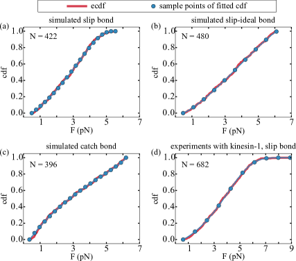
Figure S2: Fitted cumulative distributions: The red lines represent the empirical cumulative distribution functions (ecdf) constructed from simulation data of (a) slip bonds, (b) slip-ideal bonds, (c) catch bonds, and (d) from experimental data for kinesin-1. As explained in the text, we fit each ecdf by the cumulative distribution function of Eq. S15 for the respective bond behavior. To enhance the minimization algorithm, we evaluate the integrals of the cdf at a finite number of sample points shown as the blue dots.

IV Fitting of the distributions

To determine the numerical values of the free parameters for a specific unbinding behavior, we fit the analytic expressions of the unbinding force distributions to either experimental or simulated data. Because fitting a distribution directly to a histogram constructed from the data depends on the arbitrary choice of the number of bins, we instead fit the cumulative distribution functions to empirical cumulative distribution functions (ecdf) constructed from the data. For a data set of $n$ data points, the ecdf is a step function that increases by $1/n$ at each of the $n$ data points. The cumulative distribution function (cdf) is defined as

$$P(F)\equiv\int_{0}^{F}p(F^{\prime})\,dF^{\prime}.$$ (S14)

$P(F)$ is a probability and attains values between 0 and 1. To account for the limited resolution of detecting unbinding events in the experiments, we shift and renormalize the cdf with respect to the smallest detected unbinding force $F_{\rm{min}}$ of each data set to

$$P_{\rm{m}}(F)\equiv\frac{P(F)-P(F_{\rm{min}})}{1-P(F_{\rm{min}})}.$$ (S15)

For our fitting procedure, we evaluate the integrals in the cdfs only for a finite number of sample points $\{F_{i}\}$. In the case of the slip-bond data with $N=422$ detected unbinding events, we find the optimal numerical values of the parameters from the minimization

$$\min_{F_{\rm{c}},F_{\rm{d}},F_{\rm{s}}}{\sum_{i}\left({\rm ecdf}(F_{i})-P_{\rm{m}}(F_{i}|F_{\rm{c}},F_{\rm{d}},F_{\rm{s}})\right)^{2}},$$ (S16)

in which $P_{\rm{m}}(F|F_{\rm{c}},F_{\rm{d}},F_{\rm{s}})$ is given from combining Eq. S5, Eq. S14, and Eq. S15. To enhance the performance of the minimization routine in Mathematica, we restrict the intervals for the parameters to $F_{\rm{c}}\in(0,+\infty)\,\rm{pN}$, $F_{\rm{d}}\in(0,10)\,\rm{pN}$, and $F_{\rm{s}}\in(0,10)\,\rm{pN}$. We evaluate the integrals at 20 equidistant sample points $\{F_{i}\}$, see blue dots in Fig. S2. From this fitting procedure, we obtain $F_{\rm{c}}\simeq 8.32\,\rm{pN}$, $F_{\rm{d}}\simeq 3.85\,\rm{pN}$, and $F_{\rm{s}}\simeq 5.41\,\rm{pN}$. With $v_{0}\simeq 1000\,\rm{nm}/s$, $\kappa_{\rm{m}}\simeq 0.3\,\rm{pN}/\rm{nm}$ and $\kappa_{\rm{t}}\simeq 0.01\,\rm{pN}/\rm{nm}$, we determine the force-free unbinding rate

$$\epsilon_{0}=\frac{v_{0}\kappa_{\rm{m}}\kappa_{\rm{t}}}{F_{\rm{c}}(\kappa_{\rm{m}}+\kappa_{\rm{t}})}\simeq 1.16\,\rm{s}^{-1}.$$ (S17)

We obtain 95% confidence intervals with a significance of $0.05$ from a bootstrapping procedure. We re-sample 200 data sets of the original size $N=422$. For each set we determine the optimal fit parameters and calculate the lower and upper confidence interval as the 2.5 percentile and the 97.5 percentile of the distribution of each fit parameter respectively. All parameter values are listed in Table 1.

We proceed in the same way for the slip-ideal bond for which we identify $N=489$ unbinding events in the simulated data. During the minimization, we restrict the parameters to $F_{\rm{a}}\in(0.5,10)\,\rm{pN}$, $F_{\rm{c}}\in(1,5)\,\rm{pN}$, and $F_{\rm{s}}\in(1,10)\,\rm{pN}$. We evaluate the integrals at 10 equidistant sample points $\{F_{i}\}$, see blue dots in Fig. S2. The numerical values for the optimal parameters are listed in Table 1 with confidence intervals calculated in the same way as for the slip bond.

In the case of the catch bond, we determine the fit parameters as explained for the slip bond above. Our simulated data set contains $N=396$ unbinding events. To enhance the minimization, we restrict the parameter to: $F_{\rm{a}}\in(0,20)\,\rm{pN}$, $F_{\rm{c}}\in(0,20)\,\rm{pN}$, $F_{\rm{d}}\in(0,20)\,\rm{pN}$, and $F_{\rm{s}}\in(0,20)\,\rm{pN}$. We evaluate the integrals at 20 equidistant sample points $\{F_{i}\}$, see blue dots in Fig. S2. The optimal numerical values for the free parameters are listed in Table 1 with the 95% confidence intervals determined as for the two other cases.

bond behavior	parameter	value for the simulation	value from fit	CI
slip bond	$\epsilon_{0}\,(\rm{s}^{-1})$	1	1.16	[0.91; 1.62]
$\epsilon(F)=\epsilon_{0}\exp(F/F_{\rm{d}})$	$F_{\rm{d}}\,(\rm{pN})$	6	3.85	[2.51; 10.00]
	$F_{\rm{s}}\,(\rm{pN})$	6	5.41	[4.76;6.45]
slip-ideal bond	$\epsilon_{0}\,(\rm{s}^{-1})$	2	2.11	[1.94; 3.06]
$\epsilon(F)=\epsilon_{0}F/(F_{\rm{a}}+F)$	$F_{\rm{a}}\,(\rm{pN})$	1	0.84	[0.5; 5.78]
	$F_{\rm{s}}\,(\rm{pN})$	6	6.13	[3; 6.28]
catch bond	$\epsilon_{0}\,(\rm{s}^{-1})$	3	1.86	[0.86; 3.17]
$\epsilon(F)=\epsilon_{0}\exp(-F/F_{\rm{d}})+a$	$a\,(\rm{s}^{-1})$	0.5	0.75	[0.48; 1.51]
	$F_{\rm{d}}\,(\rm{pN})$	3	4.18	[0.63; 10.34]
	$F_{\rm{s}}\,(\rm{pN})$	6	6.19	[2.28; 6.26]

Table 1: Validation of distribution-based method: Each bond behavior is described by the unbinding rate $\epsilon(F)$ as given in the first column, depending on three or four parameters as listed in the second column. We choose numerical values for these parameters to generate data from our stochastic simulation. By fitting the analytic expressions for the unbinding force distributions to the generated data, we estimate the numerical values. The 95% confidence intervals are obtained from bootstrapping.

V Trace-based method

We estimate the force-dependent unbinding rate from the traces binned into $N$ force bins with bin width $\Delta F$. We label the bins with $k$, count the number $C^{\rm{un}}_{k}$ of unbinding events and the number $C^{\rm{to}}_{k}$ of points of all traces in bin $k$. Intuitively, $C^{\rm{to}}_{k}$ is the total number of possible unbinding events and $C^{\rm{un}}_{k}$ is the number of actual unbinding events. Thus, the ratio

$$\frac{C^{\rm{un}}_{k}}{C^{\rm{to}}_{k}}$$ (S18)

gives the probability of unbinding in the $k$-th bin at each sampling point in time. We divide this expression by the time step $\delta t$ between the samples to obtain the unbinding rate

$$\epsilon((k-0.5)\Delta F)=\frac{C^{\rm{un}}_{k}}{\delta tC^{\rm{to}}_{k}}.$$ (S19)

Note, the denominator $\delta tC^{\rm{to}}_{k}$ is equal to the total time of all traces spent in the $k$-th bin. This expression has been used previously to estimate the unbinding rate of molecular motors coppin1997s ; thorn2000s . In the following, we rewrite this estimator for the unbinding rate to obtain the estimator introduced by Dudko et al. dudko2008s . The number of unbinding events per bin is related to the density histogram $h_{k}$ as

$$C^{\rm{un}}_{k}=N^{\rm{un}}\Delta Fh_{k},$$ (S20)

in which $N^{\rm{un}}$ is the total number of all unbinding events. To approximate the total time that the traces spent in the $k$-th bin, we first look at all traces that pass through the bin without unbinding. The number of these traces is given by all traces that unbind after bin $k$, i.e.,

$$\sum_{i=k+1}^{N}C^{\rm{un}}_{i}.$$ (S21)

Multiplying this number by the mean time spent in the bin provides the total time of all traces passing through that bin as

$$\delta t\left\langle N^{\rm{to}}_{k}\right\rangle\sum_{i=k+1}^{N}C^{\rm{un}}_{i},$$ (S22)

in which $\left\langle N^{\rm{to}}_{k}\right\rangle$ is the mean number of data points of a trace in the bin. To account for traces that unbind at a point in $\Delta F$, we assume that they unbind uniformly in the interval $\Delta F$ and therefore the total time of these traces is given by

$$\frac{1}{2}\delta t\left\langle N^{\rm{to}}_{k}\right\rangle C^{\rm{un}}_{k}.$$ (S23)

Note that the factor $1/2$ accounts for the premature unbinding and $\left\langle N^{\rm{to}}_{k}\right\rangle$ is the mean number of data points of all traces that pass through the bin.

Taken together, the total time spent in bin $k$ reads

$$\delta tC^{\rm{to}}_{k}=\delta t\left\langle N^{\rm{to}}_{k}\right\rangle\left(\frac{1}{2}C^{\rm{un}}_{k}+\sum_{i=k+1}^{N}C^{\rm{un}}_{i}\right).$$ (S24)

To estimate the loading rate, we approximate the slope of the trace at the center of the bin as constant per bin and obtain

$$\dot{F}((k-1/2)\Delta F)=\frac{\Delta F}{\delta t\left\langle N^{\rm{to}}_{k}\right\rangle},$$ (S25)

from which we get

$$\delta t\left\langle N^{\rm{to}}_{k}\right\rangle=\frac{\Delta F}{\dot{F}((k-1/2)\Delta F)}.$$ (S26)

Combining Eq. S26, Eq. S24, Eq. S20 and Eq. S19, we derive the estimator for the unbinding rate as

$$\epsilon((k-0.5)\Delta F)=\frac{\dot{F}((k-1/2)\Delta F)h_{k}}{\Delta F(h_{k}/2+\sum_{i=k+1}^{N}h_{i})},$$ (S27)

which is the estimator proposed by Dudko in dudko2008s .

To obtain the unbinding rate with the trace-based method, we cut all traces at their unbinding events. We then bin all points of all traces according to their force and determine the number $C^{\rm{to}}_{k}$ of data points in each bin $k$. The number $C^{\rm{un}}_{k}$ of unbinding events readily follows from binning the set of unbinding forces. Together with the inverse sampling rate $\delta t^{-1}$, we obtain an estimate for the force-dependent unbinding rate from Eq. S19.

VI Kinesin-1 data

To determine the force-dependent unbinding rate for kinesin-1, we cut out $682$ single unbinding events together with the raising pulling phase. We apply the trace-based method to this data set as explained in the proceeding section. The results are discussed in the main text of the manuscript. To apply the distribution-based method to the experimental data, we determine the cumulative distribution for the slip bond by combining Eq. S5 and Eq. S15. For the fitting procedure we evaluate the integrals at 10 equidistant sample points, see blue dots in Fig. S2. We obtain the following optimal parameters with their 95% confidence intervals in brackets: $F_{\rm{c}}\simeq 15.62\,[11.26;18.9]\,\rm{pN}$, $F_{\rm{d}}\simeq 2.25\,[2.03;5.18]\,\rm{pN}$ and $F_{\rm{s}}\simeq 14.97\,[6.26;15]\,\rm{pN}$. To determine the force-free unbinding rate $\epsilon_{0}$ from Eq. S4, we use the experimental values $v_{0}\simeq 484\,\rm{nm}/\rm{s}$ and $\kappa_{\rm{t}}\simeq 0.03\,\rm{pN}/\rm{nm}$ deberg2013s . The stiffness of the molecular motor is not a crucial parameter, because the effective stiffness of the motor and the trap is governed by the smaller trap stiffness. We assume a numerical value of $\kappa_{\rm{m}}\simeq 0.3\,\rm{pN}/\rm{nm}$ coppin1997s . With these parameter values, we obtain the force-free unbinding rate $\epsilon_{0}\simeq 0.97\,[0.80;1.35]\,\rm{s}^{-1}$.

VII Estimation of variability

VII.0.1 Distribution-based method

To illustrate the variability of the data, we re-sample 200 data sets of the unbinding events and apply the fitting procedure. From each calculation we obtain a force-dependent unbinding rate. In Fig. 4 of the main text, we display the 95% of the closest unbinding rates as thin gray lines in the background.

VII.0.2 Trace-based method

To determine the 95% confidence intervals at a significance of $0.05$ we use a bootstrapping approach. We re-sample 200 data sets of unbinding events with the corresponding traces of the original size. For each data set we determine the unbinding rate from Eq. S19. Thus, we have for each sampling point of the force 200 different numerical values for the unbinding rate. We then calculate the lower and upper confidence interval as the 2.5 percentile and the 97.5 percentile of the unbinding rates at each force step.

References

- Howard (2005) J. Howard, Mechanics of Motor Proteins and the Cytoskeleton, 2005th ed. (Sinauer, Sunderland, Mass, 2005).
- Schliwa and Woehlke (2003) M. Schliwa and G. Woehlke, Nature 422, 759 (2003).
- Lipowsky and Klumpp (2005) R. Lipowsky and S. Klumpp, Physica A: Statistical Mechanics and its Applications 352, 53 (2005).
- Hunt et al. (1994) A. J. Hunt, F. Gittes, and J. Howard, Biophysical Journal 67, 766 (1994), PMID: 7948690.
- Rogers et al. (2009) A. R. Rogers, J. W. Driver, P. E. Constantinou, D. K. Jamison, and M. R. Diehl, Physical Chemistry Chemical Physics 11, 4882 (2009).
- Coppin et al. (1997) C. M. Coppin, D. W. Pierce, L. Hsu, and R. D. Vale, Proceedings of the National Academy of Sciences of the United States of America 94, 8539 (1997), PMID: 9238012 PMCID: PMC23000.
- Veigel and Schmidt (2011) C. Veigel and C. F. Schmidt, Nature Reviews Molecular Cell Biology 12, 163 (2011).
- Carter and Cross (2005) N. J. Carter and R. A. Cross, Nature 435, 308 (2005).
- Schnitzer et al. (2000) M. J. Schnitzer, K. Visscher, and S. M. Block, Nature Cell Biology 2, 718 (2000).
- Clemen et al. (2005) A. E. Clemen, M. Vilfan, J. Jaud, J. Zhang, M. Bärmann, and M. Rief, Biophysical Journal 88, 4402 (2005).
- Gennerich et al. (2007) A. Gennerich, A. P. Carter, S. L. Reck-Peterson, and R. D. Vale, Cell 131, 952 (2007).
- Andreasson et al. (2015) J. O. Andreasson, B. Milic, G. Chen, N. R. Guydosh, W. O. Hancock, and S. M. Block, eLife 4, e07403 (2015).
- Thorn et al. (2000) K. S. Thorn, J. A. Ubersax, and R. D. Vale, J Cell Biol 151, 1093 (2000), PMID: 11086010.
- Rai et al. (2013) A. K. Rai, A. Rai, A. J. Ramaiya, R. Jha, and R. Mallik, Cell 152, 172 (2013).
- Nicholas et al. (2015) M. P. Nicholas, F. Berger, L. Rao, S. Brenner, C. Cho, and A. Gennerich, Proceedings of the National Academy of Sciences 112, 6371 (2015), PMID: 25941405.
- Dudko et al. (2006) O. K. Dudko, G. Hummer, and A. Szabo, Physical Review Letters 96, 108101 (2006).
- Dudko et al. (2008) O. K. Dudko, G. Hummer, and A. Szabo, Proceedings of the National Academy of Sciences 105, 15755 (2008), PMID: 18852468.
- Klumpp et al. (2015) S. Klumpp, C. Keller, F. Berger, and R. Lipowsky, in Multiscale Modeling in Biomechanics and Mechanobiology, edited by S. De, W. Hwang, and E. Kuhl (Springer London, 2015) pp. 27–61.
- Berger (2020) See supplementary materials .
- DeBerg et al. (2013) H. A. DeBerg, B. H. Blehm, J. Sheung, A. R. Thompson, C. S. Bookwalter, S. F. Torabi, T. A. Schroer, C. L. Berger, Y. Lu, K. M. Trybus, and P. R. Selvin, The Journal of Biological Chemistry 288, 32612 (2013), PMID: 24072715 PMCID: PMC3820893.
- Arpağ et al. (2014) G. Arpağ, S. Shastry, W. O. Hancock, and E. Tüzel, Biophysical Journal 107, 1896 (2014).
- Sumi (2017) T. Sumi, Scientific Reports 7, 1163 (2017).
- Chaudhary et al. (2018) A. R. Chaudhary, F. Berger, C. L. Berger, and A. G. Hendricks, Traffic 19, 111 (2018).
- Blehm et al. (2013) B. H. Blehm, T. A. Schroer, K. M. Trybus, Y. R. Chemla, and P. R. Selvin, Proceedings of the National Academy of Sciences 110, 3381 (2013), PMID: 23404705.
- Berger et al. (2011) F. Berger, C. Keller, M. J. Müller, S. Klumpp, and R. Lipowsky, Biochemical Society Transactions 39, 1211 (2011).
- Berger et al. (2012) F. Berger, C. Keller, S. Klumpp, and R. Lipowsky, Physical Review Letters 108, 208101 (2012).
- Klumpp and Lipowsky (2005) S. Klumpp and R. Lipowsky, Proceedings of the National Academy of Sciences of the United States of America 102, 17284 (2005), PMID: 16287974.
- Müller et al. (2008) M. J. I. Müller, S. Klumpp, and R. Lipowsky, Proceedings of the National Academy of Sciences 105, 4609 (2008), PMID: 18347340.
- Berger and Hudspeth (2017) F. Berger and A. J. Hudspeth, PLOS Computational Biology 13, e1005566 (2017).
- Ruhnow et al. (2017) F. Ruhnow, L. Klo, and S. Diez, Biophysical Journal 113, 2433 (2017), PMID: 29211997.
Supplementary Materials: Force-dependent unbinding rate of
molecular motors from stationary optical trap data
Florian Berger,1 Stefan Klumpp,2 and Reinhard
Lipowsky3
1Laboratory of Sensory Neuroscience, The Rockefeller
University, New York, 10065 NY, USA
2Institute for Nonlinear Dynamics, Georg-August University
Göttingen, 37077 Göttingen, Germany
3Theory & Bio-Systems, Max Planck Institute
of Colloids and Interfaces, 14424 Potsdam, Germany
(Dated: )

References

- (1) Micah Dembo. On peeling an adherent cell from a surface. In Lectures on Mathematics in the Life Sciences, Some Mathematical Problems in Biology, pages 51–77. American Mathematical Society, Providence, RI, 1994.
- (2) Matthew P. Nicholas, Florian Berger, Lu Rao, Sibylle Brenner, Carol Cho, and Arne Gennerich. Cytoplasmic dynein regulates its attachment to microtubules via nucleotide state-switched mechanosensing at multiple AAA domains. Proceedings of the National Academy of Sciences, 112(20):6371–6376, May 2015. PMID: 25941405.
- (3) Daniel T. Gillespie. Exact stochastic simulation of coupled chemical reactions. The Journal of Physical Chemistry, 81(25):2340–2361, December 1977.
- (4) Chris M. Coppin, Daniel W. Pierce, Long Hsu, and Ronald D. Vale. The load dependence of kinesin’s mechanical cycle. Proceedings of the National Academy of Sciences of the United States of America, 94(16):8539–8544, August 1997. PMID: 9238012 PMCID: PMC23000.
- (5) Kurt S. Thorn, Jeffrey A. Ubersax, and Ronald D. Vale. Engineering the processive run length of the kinesin motor. J Cell Biol, 151(5):1093–1100, November 2000. PMID: 11086010.
- (6) Olga K. Dudko, Gerhard Hummer, and Attila Szabo. Theory, analysis, and interpretation of single-molecule force spectroscopy experiments. Proceedings of the National Academy of Sciences, 105(41):15755–15760, October 2008. PMID: 18852468.
- (7) Hannah A. DeBerg, Benjamin H. Blehm, Janet Sheung, Andrew R. Thompson, Carol S. Bookwalter, Seyed F. Torabi, Trina A. Schroer, Christopher L. Berger, Yi Lu, Kathleen M. Trybus, and Paul R. Selvin. Motor domain phosphorylation modulates kinesin-1 transport. The Journal of Biological Chemistry, 288(45):32612–32621, November 2013. PMID: 24072715 PMCID: PMC3820893.