RUDDER: Return Decomposition for Delayed Rewards

Abstract

We propose RUDDER, a novel reinforcement learning approach for delayed rewards in finite Markov decision processes (MDPs). In MDPs the $Q$-values are equal to the expected immediate reward plus the expected future rewards. The latter are related to bias problems in temporal difference (TD) learning and to high variance problems in Monte Carlo (MC) learning. Both problems are even more severe when rewards are delayed. RUDDER aims at making the expected future rewards zero, which simplifies $Q$-value estimation to computing the mean of the immediate reward. We propose the following two new concepts to push the expected future rewards toward zero. (i) Reward redistribution that leads to return-equivalent decision processes with the same optimal policies and, when optimal, zero expected future rewards. (ii) Return decomposition via contribution analysis which transforms the reinforcement learning task into a regression task at which deep learning excels. On artificial tasks with delayed rewards, RUDDER is significantly faster than MC and exponentially faster than Monte Carlo Tree Search (MCTS), TD($\lambda$), and reward shaping approaches. At Atari games, RUDDER on top of a Proximal Policy Optimization (PPO) baseline improves the scores, which is most prominent at games with delayed rewards. Source code is available at https://github.com/ml-jku/rudder and demonstration videos at https://goo.gl/EQerZV.

1 Introduction

Assigning credit for a received reward to past actions is central to reinforcement learning [128]. A great challenge is to learn long-term credit assignment for delayed rewards [65, 59, 46, 106]. Delayed rewards are often episodic or sparse and common in real-world problems [97, 76]. For Markov decision processes (MDPs), the $Q$-value is equal to the expected immediate reward plus the expected future reward. For $Q$-value estimation, the expected future reward leads to biases in temporal difference (TD) and high variance in Monte Carlo (MC) learning. For delayed rewards, TD requires exponentially many updates to correct the bias, where the number of updates is exponential in the number of delay steps. For MC learning the number of states affected by a delayed reward can grow exponentially with the number of delay steps. (Both statements are proved after theorems A8 and A10 in the appendix.) An MC estimate of the expected future reward has to average over all possible future trajectories, if rewards, state transitions, or policies are probabilistic. Delayed rewards make an MC estimate much harder.

The main goal of our approach is to construct an MDP that has expected future rewards equal to zero. If this goal is achieved, $Q$-value estimation simplifies to computing the mean of the immediate rewards. To push the expected future rewards to zero, we require two new concepts. The first new concept is reward redistribution to create return-equivalent MDPs, which are characterized by having the same optimal policies. An optimal reward redistribution should transform a delayed reward MDP into a return-equivalent MDP with zero expected future rewards. However, expected future rewards equal to zero are in general not possible for MDPs. Therefore, we introduce sequence-Markov decision processes (SDPs), for which reward distributions need not to be Markov. We construct a reward redistribution that leads to a return-equivalent SDP with a second-order Markov reward distribution and expected future rewards that are equal to zero. For these return-equivalent SDPs, $Q$-value estimation simplifies to computing the mean. Nevertheless, the $Q$-values or advantage functions can be used for learning optimal policies. The second new concept is return decomposition and its realization via contribution analysis. This concept serves to efficiently construct a proper reward redistribution, as described in the next section. Return decomposition transforms a reinforcement learning task into a regression task, where the sequence-wide return must be predicted from the whole state-action sequence. The regression task identifies which state-action pairs contribute to the return prediction and, therefore, receive a redistributed reward. Learning the regression model uses only completed episodes as training set, therefore avoids problems with unknown future state-action trajectories. Even for sub-optimal reward redistributions, we obtain an enormous speed-up of $Q$-value learning if relevant reward-causing state-action pairs are identified. We propose RUDDER (RetUrn Decomposition for DElayed Rewards) for learning with reward redistributions that are obtained via return decompositions.

To get an intuition for our approach, assume you repair pocket watches and then sell them. For a particular brand of watch you have to decide whether repairing pays off. The sales price is known, but you have unknown costs, i.e. negative rewards, caused by repair and delivery. The advantage function is the sales price minus the expected immediate repair costs minus the expected future delivery costs. Therefore, you want to know whether the advantage function is positive. — Why is zeroing the expected future costs beneficial? — If the average delivery costs are known, then they can be added to the repair costs resulting in zero future costs. Using your repairing experiences, you just have to average over the repair costs to know whether repairing pays off. — Why is return decomposition so efficient? — Because of pattern recognition. For zero future costs, you have to estimate the expected brand-related delivery costs, which are e.g. packing costs. These brand-related costs are superimposed by brand-independent general delivery costs for shipment (e.g. time spent for delivery). Assume that general delivery costs are indicated by patterns, e.g. weather conditions, which delay delivery. Using a training set of completed deliveries, supervised learning can identify these patterns and attribute costs to them. This is return decomposition. In this way, only brand-related delivery costs remain and, therefore, can be estimated more efficiently than by MC.

Related Work. Our new learning algorithm is gradually changing the reward redistribution during learning, which is known as shaping [120, 128]. In contrast to RUDDER, potential-based shaping like reward shaping [87], look-ahead advice, and look-back advice [144] use a fixed reward redistribution. Moreover, since these methods keep the original reward, the resulting reward redistribution is not optimal, as described in the next section, and learning can still be exponentially slow. A monotonic positive reward transformation [91] also changes the reward distribution but is neither assured to keep optimal policies nor to have expected future rewards of zero. Disentangled rewards keep optimal policies but are neither environment nor policy specific, therefore can in general not achieve expected future rewards being zero [28]. Successor features decouple environment and policy from rewards, but changing the reward changes the optimal policies [7, 6]. Temporal Value Transport (TVT) uses an attentional memory mechanism to learn a value function that serves as fictitious reward [59]. However, expected future rewards are not close to zero and optimal policies are not guaranteed to be kept. Reinforcement learning tasks have been changed into supervised tasks [108, 8, 112]. For example, a model that predicts the return can supply update signals for a policy by sensitivity analysis. This is known as “backpropagation through a model” [86, 101, 102, 142, 111, 4, 5]. In contrast to these approaches, (i) we use contribution analysis instead of sensitivity analysis, and (ii) we use the whole state-action sequence to predict its associated return.

2 Reward Redistribution and Novel Learning Algorithms

Reward redistribution is the main new concept to achieve expected future rewards equal to zero. We start by introducing MDPs, return-equivalent sequence-Markov decision processes (SDPs), and reward redistributions. Furthermore, optimal reward redistribution is defined and novel learning algorithms based on reward redistributions are introduced.

MDP Definitions and Return-Equivalent Sequence-Markov Decision Processes (SDPs).

A finite Markov decision process (MDP) $\mathcal{P}$ is 5-tuple $\mathcal{P}=(\mathscr{S},\mathscr{A},\mathscr{R},p,\gamma)$ of finite sets $\mathscr{S}$ of states $s$ (random variable $S_{t}$ at time $t$), $\mathscr{A}$ of actions $a$ (random variable $A_{t}$), and $\mathscr{R}$ of rewards $r$ (random variable $R_{t+1}$). Furthermore, $\mathcal{P}$ has transition-reward distributions $p(S_{t+1}=s^{\prime},R_{t+1}=r\mid S_{t}=s,A_{t}=a)$ conditioned on state-actions, and a discount factor $\gamma\in[0,1]$. The marginals are $p(r\mid s,a)=\sum_{s^{\prime}}p(s^{\prime},r\mid s,a)$ and $p(s^{\prime}\mid s,a)=\sum_{r}p(s^{\prime},r\mid s,a)$. The expected reward is $r(s,a)=\sum_{r}rp(r\mid s,a)$. The return $G_{t}$ is $G_{t}=\sum_{k=0}^{\infty}\gamma^{k}R_{t+k+1}$, while for finite horizon MDPs with sequence length $T$ and $\gamma=1$ it is $G_{t}=\sum_{k=0}^{T-t}R_{t+k+1}$. A Markov policy is given as action distribution $\pi(A_{t}=a\mid S_{t}=s)$ conditioned on states. We often equip an MDP $\mathcal{P}$ with a policy $\pi$ without explicitly mentioning it. The action-value function $q^{\pi}(s,a)$ for policy $\pi$ is $q^{\pi}(s,a)=\mathbf{\mathrm{E}}_{\pi}\left[G_{t}\mid S_{t}=s,A_{t}=a\right]$. The goal of learning is to maximize the expected return at time $t=0$, that is $v^{\pi}_{0}=\mathbf{\mathrm{E}}_{\pi}\left[G_{0}\right]$. The optimal policy $\pi^{*}$ is $\pi^{*}=\mathop{\mathrm{argmax}\,}_{\pi}[v_{0}^{\pi}]$. A sequence-Markov decision process (SDP) is defined as a decision process which is equipped with a Markov policy and has Markov transition probabilities but a reward that is not required to be Markov. Two SDPs $\tilde{\mathcal{P}}$ and $\mathcal{P}$ are return-equivalent if (i) they differ only in their reward distribution and (ii) they have the same expected return at $t=0$ for each policy $\pi$: $\tilde{v}^{\pi}_{0}=v^{\pi}_{0}$. They are strictly return-equivalent if they have the same expected return for every episode and for each policy $\pi$. Strictly return-equivalent SDPs are return-equivalent. Return-equivalent SDPs have the same optimal policies. For more details see Section A2.2 in the appendix.

Reward Redistribution.

Strictly return-equivalent SDPs $\tilde{\mathcal{P}}$ and $\mathcal{P}$ can be constructed by reward redistributions. A reward redistribution given an SDP $\tilde{\mathcal{P}}$ is a procedure that redistributes for each sequence $s_{0},a_{0},\ldots,s_{T},a_{T}$ the realization of the sequence-associated return variable $\tilde{G}_{0}=\sum_{t=0}^{T}\tilde{R}_{t+1}$ or its expectation along the sequence. Later we will introduce a reward redistribution that depends on the SDP $\tilde{\mathcal{P}}$. The reward redistribution creates a new SDP $\mathcal{P}$ with the redistributed reward $R_{t+1}$ at time $(t+1)$ and the return variable $G_{0}=\sum_{t=0}^{T}R_{t+1}$. A reward redistribution is second order Markov if the redistributed reward $R_{t+1}$ depends only on $(s_{t-1},a_{t-1},s_{t},a_{t})$. If the SDP $\mathcal{P}$ is obtained from the SDP $\tilde{\mathcal{P}}$ by reward redistribution, then $\tilde{\mathcal{P}}$ and $\mathcal{P}$ are strictly return-equivalent. The next theorem states that the optimal policies are still the same for $\tilde{\mathcal{P}}$ and $\mathcal{P}$ (proof after Section Theorem S2).

Theorem 1.

Both the SDP $\tilde{\mathcal{P}}$ with delayed reward $\tilde{R}_{t+1}$ and the SDP $\mathcal{P}$ with redistributed reward $R_{t+1}$ have the same optimal policies.

Optimal Reward Redistribution with Expected Future Rewards Equal to Zero.

We move on to the main goal of this paper: to derive an SDP via reward redistribution that has expected future rewards equal to zero and, therefore, no delayed rewards. At time $(t-1)$ the immediate reward is $R_{t}$ with expectation $r(s_{t-1},a_{t-1})$. We define the expected future rewards $\kappa(m,t-1)$ at time $(t-1)$ as the expected sum of future rewards from $R_{t+1}$ to $R_{t+1+m}$.

Definition 1.

For $1\leqslant t\leqslant T$ and $0\leqslant m\leqslant T-t$, the expected sum of delayed rewards at time $(t-1)$ in the interval $[t+1,t+m+1]$ is defined as $\kappa(m,t-1)=\mathbf{\mathrm{E}}_{\pi}\left[\sum_{\tau=0}^{m}R_{t+1+\tau}\mid s_{t-1},a_{t-1}\right]$.

For every time point $t$, the expected future rewards $\kappa(T-t-1,t)$ given $(s_{t},a_{t})$ is the expected sum of future rewards until sequence end, that is, in the interval $[t+2,T+1]$. For MDPs, the Bellman equation for $Q$-values becomes $q^{\pi}(s_{t},a_{t})=r(s_{t},a_{t})+\kappa(T-t-1,t)$. We aim to derive an MDP with $\kappa(T-t-1,t)=0$, which gives $q^{\pi}(s_{t},a_{t})=r(s_{t},a_{t})$. In this case, learning the $Q$-values simplifies to estimating the expected immediate reward $r(s_{t},a_{t})=\mathbf{\mathrm{E}}\left[R_{t+1}\mid s_{t},a_{t}\right]$. Hence, the reinforcement learning task reduces to computing the mean, e.g. the arithmetic mean, for each state-action pair $(s_{t},a_{t})$. A reward redistribution is defined to be optimal, if $\kappa(T-t-1,t)=0$ for $0\leqslant t\leqslant T-1$. In general, an optimal reward redistribution violates the Markov assumptions and the Bellman equation does not hold (proof after Theorem A3 in the appendix). Therefore, we will consider SDPs in the following. The next theorem states that a delayed reward MDP $\tilde{\mathcal{P}}$ with a particular policy $\pi$ can be transformed into a return-equivalent SDP $\mathcal{P}$ with an optimal reward redistribution.

Theorem 2.

We assume a delayed reward MDP $\tilde{\mathcal{P}}$, where the accumulated reward is given at sequence end. A new SDP $\mathcal{P}$ is obtained by a second order Markov reward redistribution, which ensures that $\mathcal{P}$ is return-equivalent to $\tilde{\mathcal{P}}$. For a specific $\pi$, the following two statements are equivalent: (I)   $\kappa(T-t-1,t)=0$, i.e. the reward redistribution is optimal,

$$\text{(II)~{}~{}}\mathbf{\mathrm{E}}\left[R_{t+1}\mid s_{t-1},a_{t-1},s_{t},a_{t}\right]\ =\ \tilde{q}^{\pi}(s_{t},a_{t})\ -\ \tilde{q}^{\pi}(s_{t-1},a_{t-1})\ .$$ (1)

An optimal reward redistribution fulfills for $1\leqslant t\leqslant T$ and $0\leqslant m\leqslant T-t$: $\kappa(m,t-1)=0$.

The proof can be found after Theorem A4 in the appendix. Equation $\kappa(T-t-1,t)=0$ implies that the new SDP $\mathcal{P}$ has no delayed rewards, that is, $\mathbf{\mathrm{E}}_{\pi}\left[R_{t+1+\tau}\mid s_{t-1},a_{t-1}\right]=0$, for $0\leqslant\tau\leqslant T-t-1$ (Corollary A1 in the appendix). The SDP $\mathcal{P}$ has no delayed rewards since no state-action pair can increase or decrease the expectation of a future reward. Equation (1) shows that for an optimal reward redistribution the expected reward has to be the difference of consecutive $Q$-values of the original delayed reward. The optimal reward redistribution is second order Markov since the expectation of $R_{t+1}$ at time $(t+1)$ depends on $(s_{t-1},a_{t-1},s_{t},a_{t})$.

The next theorem states the major advantage of an optimal reward redistribution: $\tilde{q}^{\pi}(s_{t},a_{t})$ can be estimated with an offset that depends only on $s_{t}$ by estimating the expected immediate redistributed reward. Thus, $Q$-value estimation becomes trivial and the the advantage function of the MDP $\tilde{\mathcal{P}}$ can be readily computed.

Theorem 3.

If the reward redistribution is optimal, then the $Q$-values of the SDP $\mathcal{P}$ are given by

$$q^{\pi}(s_{t},a_{t})\ =\ r(s_{t},a_{t})\ =\ \tilde{q}^{\pi}(s_{t},a_{t})\ -\ \mathbf{\mathrm{E}}_{s_{t-1},a_{t-1}}\left[\tilde{q}^{\pi}(s_{t-1},a_{t-1})\mid s_{t}\right]\ =\ \tilde{q}^{\pi}(s_{t},a_{t})\ -\ \psi^{\pi}(s_{t})\ .$$ (2)

The SDP $\mathcal{P}$ and the original MDP $\tilde{\mathcal{P}}$ have the same advantage function. Using a behavior policy $\breve{\pi}$ the expected immediate reward is

$$\mathbf{\mathrm{E}}_{\breve{\pi}}\left[R_{t+1}\mid s_{t},a_{t}\right]\ =\ \tilde{q}^{\pi}(s_{t},a_{t})\ -\ \psi^{\pi,\breve{\pi}}(s_{t})\ .$$ (3)

The proof can be found after Theorem A5 in the appendix. If the reward redistribution is not optimal, then $\kappa(T-t-1,t)$ measures the deviation of the $Q$-value from $r(s_{t},a_{t})$. This theorem justifies several learning methods based on reward redistribution presented in the next paragraph.

Novel Learning Algorithms Based on Reward Redistributions.

We assume $\gamma=1$ and a finite horizon or an absorbing state original MDP $\tilde{\mathcal{P}}$ with delayed rewards. For this setting we introduce new reinforcement learning algorithms. They are gradually changing the reward redistribution during learning and are based on the estimations in Theorem 3. These algorithms are also valid for non-optimal reward redistributions, since the optimal policies are kept (Theorem 1). Convergence of RUDDER learning can under standard assumptions be proven by the stochastic approximation for two time-scale update rules [17, 64]. Learning consists of an LSTM and a $Q$-value update. Convergence proofs to an optimal policy are difficult, since locally stable attractors may not correspond to optimal policies.

According to Theorem 1, reward redistributions keep the optimal policies. Therefore, even non-optimal reward redistributions ensure correct learning. However, an optimal reward redistribution speeds up learning considerably. Reward redistributions can be combined with methods that use $Q$-value ranks or advantage functions. We consider (A) $Q$-value estimation, (B) policy gradients, and (C) $Q$-learning. Type (A) methods estimate $Q$-values and are divided into variants (i), (ii), and (iii). Variant (i) assumes an optimal reward redistribution and estimates $\tilde{q}^{\pi}(s_{t},a_{t})$ with an offset depending only on $s_{t}$. The estimates are based on Theorem 3 either by on-policy direct $Q$-value estimation according to Eq. (2) or by off-policy immediate reward estimation according to Eq. (3). Variant (ii) methods assume a non-optimal reward redistribution and correct Eq. (2) by estimating $\kappa$. Variant (iii) methods use eligibility traces for the redistributed reward. RUDDER learning can be based on policies like “greedy in the limit with infinite exploration” (GLIE) or “restricted rank-based randomized” (RRR) [118]. GLIE policies change toward greediness with respect to the $Q$-values during learning. For more details on these learning approaches see Section A2.7.1 in the apendix.

Type (B) methods replace in the expected updates $\mathbf{\mathrm{E}}_{\pi}\left[\nabla_{\theta}\log\pi(a\mid s;\bm{\theta})q^{\pi}(s,a)\right]$ of policy gradients the value $q^{\pi}(s,a)$ by an estimate of $r(s,a)$ or by a sample of the redistributed reward. The offset $\psi^{\pi}(s)$ in Eq. (2) or $\psi^{\pi,\breve{\pi}}(s)$ in Eq. (3) reduces the variance as baseline normalization does. These methods can be extended to Trust Region Policy Optimization (TRPO) [113] as used in Proximal Policy Optimization (PPO) [115]. The type (C) method is $Q$-learning with the redistributed reward. Here, $Q$-learning is justified if immediate and future reward are drawn together, as typically done.

3 Constructing Reward Redistributions by Return Decomposition

We now propose methods to construct reward redistributions. Learning with non-optimal reward redistributions does work since the optimal policies do not change according to Theorem 1. However, reward redistributions that are optimal considerably speed up learning, since future expected rewards introduce biases in TD methods and high variances in MC methods. The expected optimal redistributed reward is the difference of $Q$-values according to Eq. (1). The more a reward redistribution deviates from these differences, the larger are the absolute $\kappa$-values and, in turn, the less optimal the reward redistribution gets. Consequently, to construct a reward redistribution which is close to optimal we aim at identifying the largest $Q$-value differences.

Reinforcement Learning as Pattern Recognition.

We want to transform the reinforcement learning problem into a pattern recognition task to employ deep learning approaches. The sum of the $Q$-value differences gives the difference between expected return at sequence begin and the expected return at sequence end (telescope sum). Thus, $Q$-value differences allow to predict the expected return of the whole state-action sequence. Identifying the largest $Q$-value differences reduces the prediction error most. $Q$-value differences are assumed to be associated with patterns in state-action transitions. The largest $Q$-value differences are expected to be found more frequently in sequences with very large or very low return. The resulting task is to predict the expected return from the whole sequence and identify which state-action transitions have contributed the most to the prediction. This pattern recognition task serves to construct a reward redistribution, where the redistributed reward corresponds to the different contributions. The next paragraph shows how the return is decomposed and redistributed along the state-action sequence.

Return Decomposition.

The return decomposition idea is that a function $g$ predicts the expectation of the return for a given state-action sequence (return for the whole sequence). The function $g$ is neither a value nor an action-value function since it predicts the expected return when the whole sequence is given. With the help of $g$ either the predicted value or the realization of the return is redistributed over the sequence. A state-action pair receives as redistributed reward its contribution to the prediction, which is determined by contribution analysis. We use contribution analysis since sensitivity analysis has serious drawbacks: local minima, instabilities, exploding or vanishing gradients, and proper exploration [48, 110]. The major drawback is that the relevance of actions is missed since sensitivity analysis does not consider the contribution of actions to the output, but only their effect on the output when slightly perturbing them. Contribution analysis determines how much a state-action pair contributes to the final prediction. We can use any contribution analysis method, but we specifically consider three methods: (A) differences of return predictions, (B) integrated gradients (IG) [125], and (C) layer-wise relevance propagation (LRP) [3]. For (A), $g$ must try to predict the sequence-wide return at every time step. The redistributed reward is given by the difference of consecutive predictions. The function $g$ can be decomposed into past, immediate, and future contributions to the return. Consecutive predictions share the same past and the same future contributions except for two immediate state-action pairs. Thus, in the difference of consecutive predictions contributions cancel except for the two immediate state-action pairs. Even for imprecise predictions of future contributions to the return, contribution analysis is more precise, since prediction errors cancel out. Methods (B) and (C) rely on information later in the sequence for determining the contribution and thereby may introduce a non-Markov reward. The reward can be viewed to be probabilistic but is prone to have high variance. Therefore, we prefer method (A).

Explaining Away Problem.

We still have to tackle the problem that reward causing actions do not receive redistributed rewards since they are explained away by later states. To describe the problem, assume an MDP $\tilde{\mathcal{P}}$ with the only reward at sequence end. To ensure the Markov property, states in $\tilde{\mathcal{P}}$ have to store the reward contributions of previous state-actions; e.g. $s_{T}$ has to store all previous contributions such that the expectation $\tilde{r}(s_{T},a_{T})$ is Markov. The explaining away problem is that later states are used for return prediction, while reward causing earlier actions are missed. To avoid explaining away, we define a difference function $\Delta(s_{t-1},a_{t-1},s_{t},a_{t})$ between a state-action pair $(s_{t},a_{t})$ and its predecessor $(s_{t-1},a_{t-1})$. That $\Delta$ is a function of $(s_{t},a_{t},s_{t-1},a_{t-1})$ is justified by Eq. (1), which ensures that such $\Delta$s allow an optimal reward redistribution. The sequence of differences is $\Delta_{0:T}:=\big{(}\Delta(s_{-1},a_{-1},s_{0},a_{0}),\ldots,\Delta(s_{T-1},a_{T-1},s_{T},a_{T})\big{)}$. The components $\Delta$ are assumed to be statistically independent from each other, therefore $\Delta$ cannot store reward contributions of previous $\Delta$. The function $g$ should predict the return by $g(\Delta_{0:T})=\tilde{r}(s_{T},a_{T})$ and can be decomposed into $g(\Delta_{0:T})=\sum_{t=0}^{T}h_{t}$. The contributions are $h_{t}=h(\Delta(s_{t-1},a_{t-1},s_{t},a_{t}))$ for $0\leqslant t\leqslant T$. For the redistributed rewards $R_{t+1}$, we ensure $\mathbf{\mathrm{E}}\left[R_{t+1}\mid s_{t-1},a_{t-1},s_{t},a_{t}\right]=h_{t}$. The reward $\tilde{R}_{T+1}$ of $\tilde{\mathcal{P}}$ is probabilistic and the function $g$ might not be perfect, therefore neither $g(\Delta_{0:T})=\tilde{r}_{T+1}$ for the return realization $\tilde{r}_{T+1}$ nor $g(\Delta_{0:T})=\tilde{r}(s_{T},a_{T})$ for the expected return holds. Therefore, we need to introduce the compensation $\tilde{r}_{T+1}\ -\ \sum_{\tau=0}^{T}h(\Delta(s_{\tau-1},a_{\tau-1},s_{\tau},a_{\tau}))$ as an extra reward $R_{T+2}$ at time $T+2$ to ensure strictly return-equivalent SDPs. If $g$ was perfect, then it would predict the expected return which could be redistributed. The new redistributed rewards $R_{t+1}$ are based on the return decomposition, since they must have the contributions $h_{t}$ as mean:
$\mathbf{\mathrm{E}}\left[R_{1}\mid s_{0},a_{0}\right]=h_{0}$ , $\mathbf{\mathrm{E}}\left[R_{t+1}\mid s_{t-1},a_{t-1},s_{t},a_{t}\right]=h_{t},0<t\leqslant T$ , $R_{T+2}=\tilde{R}_{T+1}-\sum_{t=0}^{T}h_{t}$, where the realization $\tilde{r}_{T+1}$ is replaced by its random variable $\tilde{R}_{T+1}$. If the prediction of $g$ is perfect, then we can redistribute the expected return via the prediction. Theorem 2 holds also for the correction $R_{T+2}$ (see Theorem A6 in the appendix). A $g$ with zero prediction errors results in an optimal reward redistribution. Small prediction errors lead to reward redistributions close to an optimal one.

RUDDER: Return Decomposition using LSTM.

RUDDER uses a Long Short-Term Memory (LSTM) network for return decomposition and the resulting reward redistribution. RUDDER consists of three phases. (I) Safe exploration. Exploration sequences should generate LSTM training samples with delayed rewards by avoiding low $Q$-values during a particular time interval. Low $Q$-values hint at states where the agent gets stuck. Parameters comprise starting time, length, and $Q$-value threshold. (II) Lessons replay buffer for training the LSTM. If RUDDER’s safe exploration discovers an episode with unseen delayed rewards, it is secured in a lessons replay buffer [74]. Unexpected rewards are indicated by a large prediction error of the LSTM. For LSTM training, episodes with larger errors are sampled more often from the buffer, similar to prioritized experience replay [109]. (III) LSTM and return decomposition. An LSTM learns to predict sequence-wide return at every time step and, thereafter, return decomposition uses differences of return predictions (contribution analysis method (A)) to construct a reward redistribution. For more details see Section A8.4 in the appendix.

Feedforward Neural Networks (FFNs) vs. LSTMs.

In contrast to LSTMs, FNNs are not suited for processing sequences. Nevertheless, FNNs can learn a action-value function, which enables contribution analysis by differences of predictions. However, this leads to serious problems by spurious contributions that hinder learning. For example, any contributions would be incorrect if the true expectation of the return did not change. Therefore, prediction errors might falsely cause contributions leading to spurious rewards. FNNs are prone to such prediction errors since they have to predict the expected return again and again from each different state-action pair and cannot use stored information. In contrast, the LSTM is less prone to produce spurious rewards: (i) The LSTM will only learn to store information if a state-action pair has a strong evidence for a change in the expected return. If information is stored, then internal states and, therefore, also the predictions change, otherwise the predictions stay unchanged. Hence, storing events receives a contribution and a corresponding reward, while by default nothing is stored and no contribution is given. (ii) The LSTM tends to have smaller prediction errors since it can reuse past information for predicting the expected return. For example, key events can be stored. (iii) Prediction errors of LSTMs are much more likely to cancel via prediction differences than those of FNNs. Since consecutive predictions of LSTMs rely on the same internal states, they usually have highly correlated errors.

Human Expert Episodes.

They are an alternative to exploration and can serve to fill the lessons replay buffer. Learning can be sped up considerably when LSTM identifies human key actions. Return decomposition will reward human key actions even for episodes with low return since other actions that thwart high returns receive negative reward. Using human demonstrations in reinforcement learning led to a huge improvement on some Atari games like Montezuma’s Revenge [93, 2].

Limitations.

In all of the experiments reported in this manuscript, we show that RUDDER significantly outperforms other methods for delayed reward problems. However, RUDDER might not be effective when the reward is not delayed since LSTM learning takes extra time and has problems with very long sequences. Furthermore, reward redistribution may introduce disturbing spurious reward signals.

4 Experiments

RUDDER is evaluated on three artificial tasks with delayed rewards. These tasks are designed to show problems of TD, MC, and potential-based reward shaping. RUDDER overcomes these problems. Next, we demonstrate that RUDDER also works for more complex tasks with delayed rewards. Therefore, we compare RUDDER with a Proximal Policy Optimization (PPO) baseline on 52 Atari games. All experiments use finite time horizon or absorbing states MDPs with $\gamma=1$ and reward at episode end. For more information see Section A4.1 in the appendix.

Artificial Tasks (I)–(III). Task (I) shows that TD methods have problems with vanishing information for delayed rewards. Goal is to learn that a delayed reward is larger than a distracting immediate reward. Therefore, the correct expected future reward must be assigned to many state-action pairs. Task (II) is a variation of the introductory pocket watch example with delayed rewards. It shows that MC methods have problems with the high variance of future unrelated rewards. The expected future reward that is caused by the first action has to be estimated. Large future rewards that are not associated with the first action impede MC estimations. Task (III) shows that potential-based reward shaping methods have problems with delayed rewards. For this task, only the first two actions are relevant, to which the delayed reward has to be propagated back.

The tasks have different delays, are tabular ($Q$-table), and use an $\epsilon$-greedy policy with $\epsilon=0.2$. We compare RUDDER, MC, and TD($\lambda$) on all tasks, and Monte Carlo Tree Search (MCTS) on task (I). Additionally, on task (III), SARSA($\lambda$) and reward shaping are compared. We use $\lambda=0.9$ as suggested [128]. Reward shaping methods are the original method, look-forward advice, and look-back advice with three different potential functions. RUDDER uses an LSTM without output and forget gates, no lessons buffer, and no safe exploration. For all tasks contribution analysis is performed with difference of return predictions. A $Q$-table is learned by an exponential moving average of the redistributed reward (RUDDER’s $Q$-value estimation) or by $Q$-learning. Performance is measured by the learning time to achieve 90% of the maximal expected return. A Wilcoxon signed-rank test determines the significance of performance differences between RUDDER and other methods.

(I) Grid World shows problems of TD methods with delayed rewards. The task illustrates a time bomb that explodes at episode end. The agent has to defuse the bomb and then run away as far as possible since defusing fails with a certain probability. Alternatively, the agent can immediately run away, which, however, leads to less reward on average. The Grid World is a $31\times 31$ grid with bomb at coordinate $[30,15]$ and start at $[30-d,15]$, where $d$ is the delay of the task. The agent can move up, down, left, and right as long as it stays on the grid. At the end of the episode, after $\left\lfloor 1.5d\right\rfloor$ steps, the agent receives a reward of 1000 with probability of 0.5, if it has visited bomb. At each time step, the agent receives an immediate reward of $c\cdot t\cdot h$, where $c$ depends on the chosen action, $t$ is the current time step, and $h$ is the Hamming distance to bomb. Each move toward the bomb, is immediately penalized with $c=-0.09$. Each move away from the bomb, is immediately rewarded with $c=0.1$. The agent must learn the $Q$-values precisely to recognize that directly running away is not optimal. Figure 1(I) shows the learning times to solve the task vs. the delay of the reward averaged over 100 trials. For all delays, RUDDER is significantly faster than all other methods with $p$-values $<10^{-12}$. Speed-ups vs. MC and MCTS, suggest to be exponential with delay time. RUDDER is exponentially faster with increasing delay than $Q$($\lambda$), supporting Theorem A8 in the appendix. RUDDER significantly outperforms all other methods.

Figure 1: Comparison of RUDDER and other methods on artificial tasks with respect to the learning time in episodes (median of 100 trials) vs. the delay of the reward. The shadow bands indicate the $40\%$ and $60\%$ quantiles. In (II), the y-axis of the inlet is scaled by $10^{5}$. In (III), reward shaping (RS), look-ahead advice (look-ahead), and look-back advice (look-back) use three different potential functions. In (III), the dashed blue line represents RUDDER with $Q$($\lambda$), in contrast to RUDDER with $Q$-estimation. In all tasks, RUDDER significantly outperforms all other methods.

(II) The Choice shows problems of MC methods with delayed rewards. This task has probabilistic state transitions, which can be represented as a tree with states as nodes. The agent traverses the tree from the root (initial state) to the leafs (final states). At the root, the agent has to choose between the left and the right subtree, where one subtree has a higher expected reward. Thereafter, it traverses the tree randomly according to the transition probabilities. Each visited node adds its fixed share to the final reward. The delayed reward is given as accumulated shares at a leaf. The task is solved when the agent always chooses the subtree with higher expected reward. Figure 1(II) shows the learning times to solve the task vs. the delay of the reward averaged over 100 trials. For all delays, RUDDER is significantly faster than all other methods with $p$-values $<10^{-8}$. The speed-up vs. MC, suggests to be exponential with delay time. RUDDER is exponentially faster with increasing delay than $Q$($\lambda$), supporting Theorem A8 in the appendix. RUDDER significantly outperforms all other methods.

(III) Trace-Back shows problems of potential-based reward shaping methods with delayed rewards. We investigate how fast information about delayed rewards is propagated back by RUDDER, $Q$($\lambda$), SARSA($\lambda$), and potential-based reward shaping. MC is skipped since it does not transfer back information. The agent can move in a 15$\times$15 grid to the 4 adjacent positions as long as it remains on the grid. Starting at $(7,7)$, the number of moves per episode is $T=20$. The optimal policy moves the agent up in $t=1$ and right in $t=2$, which gives immediate reward of $-50$ at $t=2$, and a delayed reward of 150 at the end $t=20=T$. Therefore, the optimal return is 100. For any other policy, the agent receives only an immediate reward of 50 at $t=2$. For $t\leqslant 2$, state transitions are deterministic, while for $t>2$ they are uniformly distributed and independent of the actions. Thus, the return does not depend on actions at $t>2$. We compare RUDDER, original reward shaping, look-ahead advice, and look-back advice. As suggested by the authors, we use SARSA instead of $Q$-learning for look-back advice. We use three different potential functions for reward shaping, which are all based on the reward redistribution (see appendix). At $t=2$, there is a distraction since the immediate reward is $-50$ for the optimal and 50 for other actions. RUDDER is significantly faster than all other methods with $p$-values $<10^{-17}$. Figure 1(III) shows the learning times averaged over 100 trials. RUDDER is exponentially faster than all other methods and significantly outperforms them.

Atari Games.

RUDDER is evaluated with respect to its learning time and achieves scores on Atari games of the Arcade Learning Environment (ALE) [11] and OpenAI Gym [18]. RUDDER is used on top of the TRPO-based [113] policy gradient method PPO that uses GAE [114]. Our PPO baseline differs from the original PPO baseline [115] in two aspects. (i) Instead of using the sign function of the rewards, rewards are scaled by their current maximum. In this way, the ratio between different rewards remains unchanged and the advantage of large delayed rewards can be recognized. (ii) The safe exploration strategy of RUDDER is used. The entropy coefficient is replaced by Proportional Control [16, 12]. A coarse hyperparameter optimization is performed for the PPO baseline. For all 52 Atari games, RUDDER uses the same architectures, losses, and hyperparameters, which were optimized for the baseline. The only difference to the PPO baseline is that the policy network predicts the value function of the redistributed reward to integrate reward redistribution into the PPO framework. Contribution analysis uses an LSTM with differences of return predictions. Here $\Delta$ is the pixel-wise difference of two consecutive frames augmented with the current frame. LSTM training and reward redistribution are restricted to sequence chunks of 500 frames. Source code is provided upon publication.

	RUDDER	baseline	delay	delay-event
Bowling	192	56	200	strike pins
Solaris	1,827	616	122	navigate map
Venture	1,350	820	150	find treasure
Seaquest	4,770	1,616	272	collect divers

Table 1: Average scores over 3 random seeds with 10 trials each for delayed reward Atari games. "delay": frames between reward and first related action. RUDDER considerably improves the PPO baseline on delayed reward games.

Policies are trained with no-op starting condition for 200M game frames using every 4th frame. Training episodes end with losing a life or at maximal 108K frames. All scores are averaged over 3 different random seeds for network and ALE initialization. We asses the performance by the learning time and the achieved scores. First, we compare RUDDER to the baseline by average scores per game throughout training, to assess learning speed [115]. For 32 (20) games RUDDER (baseline) learns on average faster. Next, we compare the average scores of the last 10 training games. For 29 (23) games RUDDER (baseline) has higher average scores. In the majority of games RUDDER, improves the scores of the PPO baseline. To compare RUDDER and the baseline on Atari games that are characterize by delayed rewards, we selected the games Bowling, Solaris, Venture, and Seaquest. In these games, high scores are achieved by learning the delayed reward, while learning the immediate reward and extensive exploration (like for Montezuma’s revenge) is less important. The results are presented in Table 1. For more details and further results see Section A4.2 in the appendix. Figure 2 displays how RUDDER redistributes rewards to key events in Bowling. At delayed reward Atari games, RUDDER considerably increases the scores compared to the PPO baseline.

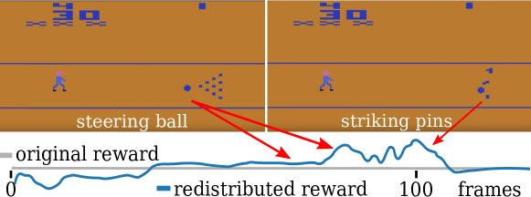
Figure 2: RUDDER redistributes rewards to key events in the Atari game Bowling. Originally, rewards are delayed and only given at episode end. The first 120 out of 200 frames of the episode are shown. RUDDER identifies key actions that steer the ball to hit all pins.

Conclusion. We have introduced RUDDER, a novel reinforcement learning algorithm based on the new concepts of reward redistribution and return decomposition. On artificial tasks, RUDDER significantly outperforms TD($\lambda$), MC, MCTS and reward shaping methods, while on Atari games it improves a PPO baseline on average but most prominently on long delayed rewards games.

Acknowledgments

This work was supported by NVIDIA Corporation, Merck KGaA, Audi.JKU Deep Learning Center, Audi Electronic Venture GmbH, Janssen Pharmaceutica (madeSMART), TGW Logistics Group, ZF Friedrichshafen AG, UCB S.A., FFG grant 871302, LIT grant DeepToxGen and AI-SNN, and FWF grant P 28660-N31.

References

References are provided in Section A11 in the appendix.

Contents

1. 1 Introduction
2. 2 Reward Redistribution and Novel Learning Algorithms
3. 3 Constructing Reward Redistributions by Return Decomposition
4. 4 Experiments
5. A1 Definition of Finite Markov Decision Processes
6. A2 Reward Redistribution, Return-Equivalent SDPs, Novel Learning Algorithms, and Return Decomposition
   1. A2.1 State Enriched MDPs
   2. A2.2 Return-Equivalent Sequence-Markov Decision Processes (SDPs)
      1. A2.2.1 Sequence-Markov Decision Processes (SDPs)
      2. A2.2.2 Return-Equivalent SDPs
   3. A2.3 Reward Redistribution for Strictly Return-Equivalent SDPs
      1. A2.3.1 Reward Redistribution
   4. A2.4 Reward Redistribution Constructs Strictly Return-Equivalent SDPs
      1. A2.4.1 Special Cases of Strictly Return-Equivalent Decision Processes: Reward Shaping, Look-Ahead Advice, and Look-Back Advice
   5. A2.5 Transforming an Immediate Reward MDP to a Delayed Reward MDP
   6. A2.6 Transforming an Delayed Reward MDP to an Immediate Reward SDP
      1. A2.6.1 Optimal Reward Redistribution
   7. A2.7 Novel Learning Algorithms based on Reward Redistributions
      1. A2.7.1 Q-Value Estimation
      2. A2.7.2 Policy Gradients
      3. A2.7.3 Q-Learning
   8. A2.8 Return Decomposition to construct a Reward Redistribution
      1. A2.8.1 Return Decomposition Idea
      2. A2.8.2 Reward Redistribution based on Return Decomposition
   9. A2.9 Remarks on Return Decomposition
      1. A2.9.1 Return Decomposition for Binary Reward
      2. A2.9.2 Optimal Reward Redistribution reduces the MDP to a Stochastic Contextual Bandit Problem
      3. A2.9.3 Relation to ”Backpropagation through a Model´´
7. A3 Bias-Variance Analysis of MDP Q-Value Estimators
   1. A3.1 Bias-Variance for MC and TD Estimates of the Expected Return
   2. A3.2 Mean and Variance of an MDP Sample of the Return
   3. A3.3 TD corrects Bias exponentially slowly with Respect to Reward Delay
   4. A3.4 MC affects the Variance of Exponentially Many Estimates with Delayed Reward
8. A4 Experiments
   1. A4.1 Artificial Tasks
      1. A4.1.1 Task (I): Grid World
      2. A4.1.2 Task (II): The Choice
      3. A4.1.3 Task(III): Trace-Back
      4. A4.1.4 Task (IV): Charge-Discharge
      5. A4.1.5 Task (V): Solving Trace-Back using policy gradient methods
   2. A4.2 Atari Games
      1. A4.2.1 Architecture
      2. A4.2.2 Lessons Replay Buffer
      3. A4.2.3 Game Processing, Update Design, and Target Design
      4. A4.2.4 Exploration
      5. A4.2.5 Results
         1. A5 Discussion and Frequent Questions
            1. A6 Additional Related Work
               1. A7 Markov Decision Processes with Undiscounted Rewards
                  1. A7.1 Properties of the Bellman Operator in MDPs with Undiscounted Rewards
                     1. A7.1.1 Monotonically Increasing and Continuous
                     2. A7.1.2 Contraction for Undiscounted Finite Horizon
                     3. A7.1.3 Contraction for Undiscounted Infinite Horizon With Absorbing States
                     4. A7.1.4 Fixed Point of Contraction is Continuous wrt Parameters
                     5. A7.1.5 t-fold Composition of the Operator
                  2. A7.2 Q-value Transformations: Shaping Reward, Baseline, and Normalization
                  3. A7.3 Alternative Definition of State Enrichment
                  4. A7.4 Variance of the Weighted Sum of a Multinomial Distribution
                  5. A8 Long Short-Term Memory (LSTM)
                     1. A8.1 LSTM Introduction
                     2. A8.2 LSTM in a Nutshell
                     3. A8.3 Long-Term Dependencies vs. Uniform Credit Assignment
                     4. A8.4 Special LSTM Architectures for contribution Analysis
                        1. A8.4.1 LSTM for Integrated Gradients
                        2. A8.4.2 LSTM for LRP
                        3. A8.4.3 LSTM for Nondecreasing Memory Cells
                        4. A8.4.4 LSTM without Gates
                     5. A9 Contribution Analysis
                        1. A9.1 Difference of Consecutive Predictions for Sequences
                        2. A9.2 Input Zeroing
                        3. A9.3 Integrated Gradients
                        4. A9.4 Layer-Wise Relevance Propagation
                           1. A9.4.1 New Variants of LRP
                           2. A9.4.2 LRP for Products
                        5. A9.5 Variance Considerations for contribution Analysis
                        6. A10 Reproducibility Checklist
                           1. A11 References

Appendix A1 Definition of Finite Markov Decision Processes

We consider a finite Markov decision process (MDP) $\mathcal{P}$, which is a 5-tuple $\mathcal{P}=(\mathscr{S},\mathscr{A},\mathscr{R},p,\gamma)$:

• $\mathscr{S}$ is a finite set of states; $S_{t}$ is the random variable for states at time $t$ with value $s\in\mathscr{S}$. $S_{t}$ has a discrete probability distribution.

• $\mathscr{A}$ is a finite set of actions (sometimes state-dependent $\mathscr{A}(s)$); $A_{t}$ is the random variable for actions at time $t$ with value $a\in\mathscr{A}$. $A_{t}$ has a discrete probability distribution.

• $\mathscr{R}$ is a finite set of rewards; $R_{t+1}$ is the random variable for rewards at time $(t+1)$ with value $r\in\mathscr{R}$. $R_{t}$ has a discrete probability distribution.

• $p(S_{t+1}=s^{\prime},R_{t+1}=r\mid S_{t}=s,A_{t}=a)$ are the transition and reward distributions over states and rewards, respectively, conditioned on state-actions,

• $\gamma\in[0,1]$ is a discount factor for the reward.

The Markov policy $\pi$ is a distribution over actions given the state: $\pi(A_{t}=a\mid S_{t}=s)$. We often equip an MDP $\mathcal{P}$ with a policy $\pi$ without explicitly mentioning it. At time $t$, the random variables give the states, actions, and rewards of the MDP, while low-case letters give possible values. At each time $t$, the environment is in some state $s_{t}\in\mathscr{S}$. The policy $\pi$ takes an action $a_{t}\in\mathscr{A}$, which causes a transition of the environment to state $s_{t+1}$ and a reward $r_{t+1}$ for the policy. Therefore, the MDP creates a sequence

$$\left(S_{0},A_{0},R_{1},S_{1},A_{1},R_{2},S_{2},A_{2},R_{3},\ldots\right)\ .$$ (A1)

The marginal probabilities for

$$p(s^{\prime},r\mid s,a)\ =\ \mathbf{\mathrm{Pr}}\left[S_{t+1}=s^{\prime},R_{t+1}=r\mid S_{t}=s,A_{t}=a\right]\$$ (A2)

are:

$$p(r\mid s,a)\ =\ \mathbf{\mathrm{Pr}}\left[R_{t+1}=r\mid S_{t}=s,A_{t}=a\right]\ =\ \sum_{s^{\prime}}p(s^{\prime},r\mid s,a)\ ,$$ (A3)

$$p(s^{\prime}\mid s,a)\ =\ \mathbf{\mathrm{Pr}}\left[S_{t+1}=s^{\prime}\mid S_{t}=s,A_{t}=a\right]\ =\ \sum_{r}p(s^{\prime},r\mid s,a)\ .$$ (A4)

We use a sum convention: $\sum_{a,b}$ goes over all possible values of $a$ and $b$, that is, all combinations which fulfill the constraints on $a$ and $b$. If $b$ is a function of $a$ (fully determined by $a$), then $\sum_{a,b}=\sum_{a}$.

We denote expectations:

• $\mathbf{\mathrm{E}}_{\pi}$ is the expectation where the random variable is an MDP sequence of states, actions, and rewards generated with policy $\pi$.

• $\mathbf{\mathrm{E}}_{s}$ is the expectation where the random variable is $S_{t}$ with values $s\in\mathscr{S}$.

• $\mathbf{\mathrm{E}}_{a}$ is the expectation where the random variable is $A_{t}$ with values $a\in\mathscr{A}$.

• $\mathbf{\mathrm{E}}_{r}$ is the expectation where the random variable is $R_{t+1}$ with values $r\in\mathscr{R}$.

• $\mathbf{\mathrm{E}}_{s,a,r,s^{\prime},a^{\prime}}$ is the expectation where the random variables are $S_{t+1}$ with values $s^{\prime}\in\mathscr{S}$, $S_{t}$ with values $s\in\mathscr{S}$, $A_{t}$ with values $a\in\mathscr{A}$, $A_{t+1}$ with values $a^{\prime}\in\mathscr{A}$, and $R_{t+1}$ with values $r\in\mathscr{R}$. If more or fewer random variables are used, the notation is consistently adapted.

The return $G_{t}$ is the accumulated reward starting from $t+1$:

$$G_{t}\ =\ \sum_{k=0}^{\infty}\gamma^{k}\ R_{t+k+1}\ .$$ (A5)

The discount factor $\gamma$ determines how much immediate rewards are favored over more delayed rewards. For $\gamma=0$ the return (the objective) is determined as the largest expected immediate reward, while for $\gamma=1$ the return is determined by the expected sum of future rewards if the sum exists.

State-Value and Action-Value Function.

The state-value function $v^{\pi}(s)$ for policy $\pi$ and state $s$ is defined as

$$v^{\pi}(s)\ =\ \mathbf{\mathrm{E}}_{\pi}\left[G_{t}\mid S_{t}=s\right]\ =\ \mathbf{\mathrm{E}}_{\pi}\left[\sum_{k=0}^{\infty}\gamma^{k}\ R_{t+k+1}\mid S_{t}=s\right]\ .$$ (A6)

Starting at $t=0$:

$$v_{0}^{\pi}\ =\ \mathbf{\mathrm{E}}_{\pi}\left[\sum_{t=0}^{\infty}\gamma^{t}\ R_{t+1}\right]\ =\ \mathbf{\mathrm{E}}_{\pi}\left[G_{0}\right]\ ,$$ (A7)

the optimal state-value function $v_{*}$ and policy $\pi_{*}$ are

$$v_{*}(s)\ =\ \max_{\pi}v^{\pi}(s)\ ,$$ (A8)

$$\pi_{*}\ =\ \arg\max_{\pi}v^{\pi}(s)\ \text{ for all }s\ .$$ (A9)

The action-value function $q^{\pi}(s,a)$ for policy $\pi$ is the expected return when starting from $S_{t}=s$, taking action $A_{t}=a$, and following policy $\pi$:

$$q^{\pi}(s,a)\ =\ \mathbf{\mathrm{E}}_{\pi}\left[G_{t}\mid S_{t}=s,A_{t}=a\right]\ =\ \mathbf{\mathrm{E}}_{\pi}\left[\sum_{k=0}^{\infty}\gamma^{k}\ R_{t+k+1}\mid S_{t}=s,A_{t}=a\right]\ .$$ (A10)

The optimal action-value function $q_{*}$ and policy $\pi_{*}$ are

$$q_{*}(s,a)\ =\ \max_{\pi}q^{\pi}(s,a)\ ,$$ (A11)

$$\pi_{*}\ =\ \arg\max_{\pi}q^{\pi}(s,a)\ \text{ for all }(s,a)\ .$$ (A12)

The optimal action-value function $q_{*}$ can be expressed via the optimal value function $v_{*}$:

$$q_{*}(s,a)\ =\ \mathbf{\mathrm{E}}\left[R_{t+1}\ +\ \gamma\ v_{*}(S_{t+1})\mid S_{t}=s,A_{t}=a\right]\ .$$ (A13)

The optimal state-value function $v_{*}$ can be expressed via the optimal action-value function $q_{*}$ using the optimal policy $\pi_{*}$:

$$v_{*}(s)\ =\ \max_{a}q^{\pi_{*}}(s,a)\ =\ \max_{a}\mathbf{\mathrm{E}}_{\pi_{*}}\left[G_{t}\mid S_{t}=s,A_{t}=a\right]\ =$$ (A14)

$$\max_{a}\mathbf{\mathrm{E}}_{\pi_{*}}\left[R_{t+1}\ +\ \gamma\ G_{t+1}\mid S_{t}=s,A_{t}=a\right]\ =$$

$$\max_{a}\mathbf{\mathrm{E}}\left[R_{t+1}\ +\ \gamma\ v_{*}(S_{t+1})\mid S_{t}=s,A_{t}=a\right]\ .$$

Finite time horizon and no discount.

We consider a finite time horizon, that is, we consider only episodes of length $T$, but may receive reward $R_{T+1}$ at episode end at time $T+1$. The finite time horizon MDP creates a sequence

$$\left(S_{0},A_{0},R_{1},S_{1},A_{1},R_{2},S_{2},A_{2},R_{3},\ldots,S_{T-1},A_{T-1},R_{T},S_{T},A_{T},R_{T+1}\right)\ .$$ (A15)

Furthermore, we do not discount future rewards, that is, we set $\gamma=1$. The return $G_{t}$ from time $t$ to $T$ is the sum of rewards:

$$G_{t}\ =\ \sum_{k=0}^{T-t}R_{t+k+1}\ .$$ (A16)

The state-value function $v$ for policy $\pi$ is

$$v^{\pi}(s)\ =\ \mathbf{\mathrm{E}}_{\pi}\left[G_{t}\mid S_{t}=s\right]\ =\ \mathbf{\mathrm{E}}_{\pi}\left[\sum_{k=0}^{T-t}R_{t+k+1}\mid S_{t}=s\right]$$ (A17)

and the action-value function $q$ for policy $\pi$ is

$$q^{\pi}(s,a)\ =\ \mathbf{\mathrm{E}}_{\pi}\left[G_{t}\mid S_{t}=s,A_{t}=a\right]\ =\ \mathbf{\mathrm{E}}_{\pi}\left[\sum_{k=0}^{T-t}R_{t+k+1}\mid S_{t}=s,A_{t}=a\right]$$ (A18)

$$=\ \mathbf{\mathrm{E}}_{\pi}\left[R_{t+1}\ +\ G_{t+1}\mid S_{t}=s,A_{t}=a\right]$$

$$=\ \sum_{s^{\prime},r}p(s^{\prime},r\mid s,a)\left[r\ +\ \sum_{a^{\prime}}\pi(a^{\prime}\mid s^{\prime})\ q^{\pi}(s^{\prime},a^{\prime})\right]\ .$$

From the Bellman equation Eq. (A18), we obtain:

$$\sum_{s^{\prime}}p(s^{\prime}\mid s,a)\ \sum_{a^{\prime}}\pi(a^{\prime}\mid s^{\prime})\ q^{\pi}(s^{\prime},a^{\prime})\ =\ q^{\pi}(s,a)\ -\ \sum_{r}r\ p(r\mid s,a)\ ,$$ (A19)

$$\mathbf{\mathrm{E}}_{s^{\prime},a^{\prime}}\left[q^{\pi}(s^{\prime},a^{\prime})\mid s,a\right]\ =\ q^{\pi}(s,a)\ -\ r(s,a)\ .$$ (A20)

The expected return at time $t=0$ for policy $\pi$ is

$$v_{0}^{\pi}\ =\ \mathbf{\mathrm{E}}_{\pi}\left[G_{0}\right]\ =\ \mathbf{\mathrm{E}}_{\pi}\left[\sum_{t=0}^{T}R_{t+1}\right]\ ,$$ (A21)

$$\pi^{*}\ =\ \underset{\pi}{\mathop{\mathrm{argmax}\,}}\ v_{0}^{\pi}\ .$$

The agent may start in a particular starting state $S_{0}$ which is a random variable. Often $S_{0}$ has only one value $s_{0}$.

Learning.

The goal of learning is to find the policy $\pi^{*}$ that maximizes the expected future discounted reward (the return) if starting at $t=0$. Thus, the optimal policy $\pi^{*}$ is

$$\pi^{*}\ =\ \underset{\pi}{\mathop{\mathrm{argmax}\,}}\ v_{0}^{\pi}\ .$$ (A22)

We consider two learning approaches for $Q$-values: Monte Carlo and temporal difference.

Monte Carlo (MC).

To estimate $q^{\pi}(s,a)$, MC computes the arithmetic mean of all observed returns $(G_{t}\mid S_{t}=s,A_{t}=a)$ in the data. When using Monte Carlo for learning a policy we use an exponentially weighted arithmetic mean since the policy steadily changes.

For the $i$th update Monte Carlo tries to minimize $\frac{1}{2}M(s_{t},a_{t})^{2}$ with the residual $M(s_{t},a_{t})$

$$M(s_{t},a_{t})\ =\ (q^{\pi})^{i}(s_{t},a_{t})\ -\ \sum_{\tau=0}^{T-t-1}\gamma^{\tau}r_{t+1+\tau}\ ,$$ (A23)

such that the update of the action-value $q$ at state-action $(s_{t},a_{t})$ is

$$(q^{\pi})^{i+1}(s_{t},a_{t})\ =\ (q^{\pi})^{i}(s_{t},a_{t})\ -\ \alpha\ M(s_{t},a_{t})\ .$$ (A24)

This update is called constant-$\alpha$ MC [128].

Temporal difference (TD) methods.

TD updates are based on the Bellman equation. If $r(s,a)$ and $\mathbf{\mathrm{E}}_{s^{\prime},a^{\prime}}\left[\hat{q}^{\pi}(s^{\prime},a^{\prime})\mid s,a\right]$ have been estimated, the $Q$-values can be updated according to the Bellman equation:

$$\left(\hat{q}^{\pi}\right)^{\mathrm{new}}(s,a)\ =\ r(s,a)\ +\ \gamma\ \mathbf{\mathrm{E}}_{s^{\prime},a^{\prime}}\left[\hat{q}^{\pi}(s^{\prime},a^{\prime})\mid s,a\right]\ .$$ (A25)

The update is applying the Bellman operator with estimates $\mathbf{\mathrm{E}}_{s^{\prime},a^{\prime}}\left[\hat{q}^{\pi}(s^{\prime},a^{\prime})\mid s,a\right]$ and $r(s,a)$ to $\hat{q}^{\pi}$ to obtain $\left(\hat{q}^{\pi}\right)^{\mathrm{new}}$. The new estimate $\left(\hat{q}^{\pi}\right)^{\mathrm{new}}$ is closer to the fixed point $q^{\pi}$ of the Bellman operator, since the Bellman operator is a contraction (see Section A7.1.3 and Section A7.1.2).

Since the estimates $\mathbf{\mathrm{E}}_{s^{\prime},a^{\prime}}\left[\hat{q}^{\pi}(s^{\prime},a^{\prime})\mid s,a\right]$ and $r(s,a)$ are not known, TD methods try to minimize $\frac{1}{2}B(s,a)^{2}$ with the Bellman residual $B(s,a)$:

$$B(s,a)\ =\ \hat{q}^{\pi}(s,a)\ -\ r(s,a)\ -\ \gamma\ \mathbf{\mathrm{E}}_{s^{\prime},a^{\prime}}\left[\hat{q}^{\pi}(s^{\prime},a^{\prime})\right]\ .$$ (A26)

TD methods use an estimate $\hat{B}(s,a)$ of $B(s,a)$ and a learning rate $\alpha$ to make an update

$$\hat{q}^{\pi}(s,a)^{\mathrm{new}}\ \leftarrow\ \hat{q}^{\pi}(s,a)\ -\ \alpha\ \hat{B}(s,a)\ .$$ (A27)

For all TD methods $r(s,a)$ is estimated by $R_{t+1}$ and $s^{\prime}$ by $S_{t+1}$, while $\hat{q}^{\pi}(s^{\prime},a^{\prime})$ does not change with the current sample, that is, it is fixed for the estimate. However, the sample determines which $(s^{\prime},a^{\prime})$ is chosen. The TD methods differ in how they select $a^{\prime}$. SARSA [105] selects $a^{\prime}$ by sampling from the policy:

$$\mathbf{\mathrm{E}}_{s^{\prime},a^{\prime}}\left[\hat{q}^{\pi}(s^{\prime},a^{\prime})\right]\ \approx\ \hat{q}^{\pi}(S_{t+1},A_{t+1})$$

and expected SARSA [63] averages over selections

$$\mathbf{\mathrm{E}}_{s^{\prime},a^{\prime}}\left[\hat{q}^{\pi}(s^{\prime},a^{\prime})\right]\ \approx\ \sum_{a}\pi(a\mid S_{t+1})\ \hat{q}^{\pi}(S_{t+1},a).$$

It is possible to estimate $r(s,a)$ separately via an unbiased minimal variance estimator like the arithmetic mean and then perform TD updates with the Bellman error using the estimated $r(s,a)$ [103]. $\bm{Q}$-learning [140] is an off-policy TD algorithm which is proved to converge [141, 20]. The proofs were later generalized [61, 133]. $Q$-learning uses

$$\mathbf{\mathrm{E}}_{s^{\prime},a^{\prime}}\left[\hat{q}^{\pi}(s^{\prime},a^{\prime})\right]\ \approx\ \max_{a}\hat{q}(S_{t+1},a)\ .$$ (A28)

The action-value function $q$, which is learned by $Q$-learning, approximates $q_{*}$ independently of the policy that is followed. More precisely, with $Q$-learning $q$ converges with probability 1 to the optimal $q_{*}$. However, the policy still determines which state-action pairs are encountered during learning. The convergence only requires that all action-state pairs are visited and updated infinitely often.

Appendix A2 Reward Redistribution, Return-Equivalent SDPs, Novel Learning Algorithms, and Return Decomposition

A2.1 State Enriched MDPs

For MDPs with a delayed reward the states have to code the reward. However, for an immediate reward the states can be made more compact by removing the reward information. For example, states with memory of a delayed reward can be mapped to states without memory. Therefore, in order to compare MDPs, we introduce the concept of homomorphic MDPs. We first need to define a partition of a set induced by a function. Let $B$ be a partition of a set $X$. For any $x\in X$, we denote $[x]_{B}$ the block of $B$ to which $x$ belongs. Any function $f$ from a set $X$ to a set $Y$ induces a partition (or equivalence relation) on $X$, with $[x]_{f}=[x^{\prime}]_{f}$ if and only if $f(x)=f(x^{\prime})$. We now can define homomorphic MDPs.

Definition A1 (Ravindran and Barto [98, 99]).

An MDP homomorphism $h$ from an MDP $\mathcal{P}=(\mathscr{S},\mathscr{A},\mathscr{R},p,\gamma)$ to an MDP $\tilde{\mathcal{P}}=(\tilde{\mathscr{S}},\tilde{\mathscr{A}},\tilde{\mathscr{R}},\tilde{p},\tilde{\gamma})$ is a a tuple of surjections $(f,g_{1},g_{2},\ldots,g_{n})$ ($n$ is number of states), with $h(s,a)=(f(s),g_{s}(a))$, where $f:\mathscr{S}\to\tilde{\mathscr{S}}$ and $g_{s}:\mathscr{A}_{s}\to\tilde{\mathscr{A}}_{f(s)}$ for $s\in\mathscr{S}$ ($\mathscr{A}_{s}$ are the admissible actions in state $s$ and $\tilde{\mathscr{A}}_{f(s)}$ are the admissible actions in state $\tilde{s}$). Furthermore, for all $s,s^{\prime}\in\mathscr{S},a\in\mathscr{A}_{s}$:

$$\tilde{p}(f(s^{\prime})\mid f(s),g_{s}(a))\ =\ \sum_{s^{\prime\prime}\in[s^{\prime}]_{f}}p(s^{\prime\prime}\mid s,a)\ ,$$ (A29)

$$\tilde{p}(\tilde{r}\mid f(s),g_{s}(a))\ =\ p(r\mid s,a)\ .$$ (A30)

We use $[s]_{f}=[s^{\prime}]_{f}$ if and only if $f(s)=f(s^{\prime})$.

We call $\tilde{\mathcal{P}}$ the homomorphic image of $\mathcal{P}$ under $h$. For homomorphic images the optimal $Q$-values and the optimal policies are the same.

Lemma A1 (Ravindran and Barto [98]).

If $\tilde{\mathcal{P}}$ is a homomorphic image of $\mathcal{P}$, then the optimal $Q$-values are the same and a policy that is optimal in $\tilde{\mathcal{P}}$ can be transformed to an optimal policy in $\mathcal{P}$ by normalizing the number of actions $a$ that are mapped to the same action $\tilde{a}$.

Consequently, the original MDP can be solved by solving a homomorphic image.

Similar results have been obtained by Givan et al. using stochastically bisimilar MDPs: “Any stochastic bisimulation used for aggregation preserves the optimal value and action sequence properties as well as the optimal policies of the model” [34]. Theorem 7 and Corollary 9.1 in Givan et al. show the facts of Lemma A1. Li et al. give an overview over state abstraction and state aggregation for Markov decision processes, which covers homomorphic MDPs [73].

A Markov decision process $\tilde{\mathcal{P}}$ is state-enriched compared to an MDP $\mathcal{P}$ if $\tilde{\mathcal{P}}$ has the same states, actions, transition probabilities, and reward probabilities as $\mathcal{P}$ but with additional information in its states. We define state-enrichment as follows:

Definition A2.

A Markov decision process $\tilde{\mathcal{P}}$ is state-enriched compared to a Markov decision process $\mathcal{P}$ if $\mathcal{P}$ is a homomorphic image of $\tilde{\mathcal{P}}$, where $g_{\tilde{s}}$ is the identity and $f(\tilde{s})=s$ is not bijective.

Being not bijective means that there exist $\tilde{s}^{\prime}$ and $\tilde{s}^{\prime\prime}$ with $f(\tilde{s}^{\prime})=f(\tilde{s}^{\prime\prime})$, that is, $\tilde{\mathscr{S}}$ has more elements than $\mathscr{S}$. In particular, state-enrichment does not change the optimal policies nor the $Q$-values in the sense of Lemma A1.

Proposition A1.

If an MDP $\tilde{\mathcal{P}}$ is state-enriched compared to an MDP $\mathcal{P}$, then both MDPs have the same optimal $Q$-values and the same optimal policies.

Proof.

According to the definition $\mathcal{P}$ is a homomorphic image of $\tilde{\mathcal{P}}$. The statements of Proposition A1 follow directly from Lemma A1. ∎

Optimal policies of the state-enriched MDP $\tilde{\mathcal{P}}$ can be transformed to optimal policies of the original MDP $\mathcal{P}$ and, vice versa, each optimal policy of the original MDP $\mathcal{P}$ corresponds to at least one optimal policy of the state-enriched MDP $\tilde{\mathcal{P}}$.

A2.2 Return-Equivalent Sequence-Markov Decision Processes (SDPs)

Our goal is to compare Markov decision processes (MDPs) with delayed rewards to decision processes (DPs) without delayed rewards. The DPs without delayed rewards can but need not to be Markov in the rewards. Toward this end, we consider two DPs $\tilde{\mathcal{P}}$ and $\mathcal{P}$ which differ only in their (non-Markov) reward distributions. However for each policy $\pi$ the DPs $\tilde{\mathcal{P}}$ and $\mathcal{P}$ have the same expected return at $t=0$, that is, $\tilde{v}^{\pi}_{0}=v^{\pi}_{0}$, or they have the same expected return for every episode.

A2.2.1 Sequence-Markov Decision Processes (SDPs)

We first define decision processes that are Markov except for the reward, which is not required to be Markov.

Definition A3.

A sequence-Markov decision process (SDP) is defined as a finite decision process which is equipped with a Markov policy and has Markov transition probabilities but a reward distribution that is not required to be Markov.

Proposition A2.

Markov decision processes are sequence-Markov decision processes.

Proof.

MDPs have Markov transition probabilities and are equipped with Markov policies. ∎

Definition A4.

We call two sequence-Markov decision processes $\mathcal{P}$ and $\tilde{\mathcal{P}}$ that have the same Markov transition probabilities and are equipped with the same Markov policy sequence-equivalent.

Lemma A2.

Two sequence-Markov decision processes that are sequence-equivalent have the same probability to generate state-action sequences $(s_{0},a_{0},\ldots,s_{t},a_{t})$, $0\leqslant t\leqslant T$.

Proof.

Sequence generation only depends on transition probabilities and policy. Therefore the probability of generating a particular sequences is the same for both SDPs. ∎

A2.2.2 Return-Equivalent SDPs

We define return-equivalent SDPs which can be shown to have the same optimal policies.

Definition A5.

Two sequence-Markov decision processes $\tilde{\mathcal{P}}$ and $\mathcal{P}$ are return-equivalent if they differ only in their reward but for each policy $\pi$ have the same expected return $\tilde{v}^{\pi}_{0}=v^{\pi}_{0}$. $\tilde{\mathcal{P}}$ and $\mathcal{P}$ are strictly return-equivalent if they have the same expected return for every episode and for each policy $\pi$:

$$\mathbf{\mathrm{E}}_{\pi}\left[\tilde{G}_{0}\mid s_{0},a_{0},\ldots,s_{T},a_{T}\right]\ =\ \mathbf{\mathrm{E}}_{\pi}\left[G_{0}\mid s_{0},a_{0},\ldots,s_{T},a_{T}\right]\ .$$ (A31)

The definition of return-equivalence can be generalized to strictly monotonic functions $f$ for which $\tilde{v}^{\pi}_{0}=f(v^{\pi}_{0})$. Since strictly monotonic functions do not change the ordering of the returns, maximal returns stay maximal after applying the function $f$.

Strictly return-equivalent SDPs are return-equivalent as the next proposition states.

Proposition A3.

Strictly return-equivalent sequence-Markov decision processes are return-equivalent.

Proof.

The expected return at $t=0$ given a policy is the sum of the probability of generating a sequence times the expected reward for this sequence. Both expectations are the same for two strictly return-equivalent sequence-Markov decision processes. Therefore the expected return at time $t=0$ is the same. ∎

The next proposition states that return-equivalent SDPs have the same optimal policies.

Proposition A4.

Return-equivalent sequence-Markov decision processes have the same optimal policies.

Proof.

The optimal policy is defined as maximizing the expected return at time $t=0$. For each policy the expected return at time $t=0$ is the same for return-equivalent decision processes. Consequently, the optimal policies are the same. ∎

Two strictly return-equivalent SDPs have the same expected return for each state-action sub-sequence $(s_{0},a_{0},\ldots,s_{t},a_{t})$, $0\leqslant t\leqslant T$.

Lemma A3.

Two strictly return-equivalent SDPs $\tilde{\mathcal{P}}$ and $\mathcal{P}$ have the same expected return for each state-action sub-sequence $(s_{0},a_{0},\ldots,s_{t},a_{t})$, $0\leqslant t\leqslant T$:

$$\mathbf{\mathrm{E}}_{\pi}\left[\tilde{G}_{0}\mid s_{0},a_{0},\ldots,s_{t},a_{t}\right]\ =\ \mathbf{\mathrm{E}}_{\pi}\left[G_{0}\mid s_{0},a_{0},\ldots,s_{t},a_{t}\right]\ .$$ (A32)

Proof.

Since the SDPs are strictly return-equivalent, we have

$$\mathbf{\mathrm{E}}_{\pi}\left[\tilde{G}_{0}\mid s_{0},a_{0},\ldots,s_{t},a_{t}\right]$$ (A33)

$$=\ \sum_{s_{t+1},a_{t+1},\ldots,s_{T},a_{T}}p_{\pi}(s_{t+1},a_{t+1},\ldots,s_{T},a_{T}\mid s_{t},a_{t})\ \mathbf{\mathrm{E}}_{\pi}\left[\tilde{G}_{0}\mid s_{0},a_{0},\ldots,s_{T},a_{T}\right]$$

$$=\ \sum_{s_{t+1},a_{t+1},\ldots,s_{T},a_{T}}p_{\pi}(s_{t+1},a_{t+1},\ldots,s_{T},a_{T}\mid s_{t},a_{t})\ \mathbf{\mathrm{E}}_{\pi}\left[G_{0}\mid s_{0},a_{0},\ldots,s_{T},a_{T}\right]$$

$$=\ \mathbf{\mathrm{E}}_{\pi}\left[G_{0}\mid s_{0},a_{0},\ldots,s_{t},a_{t}\right]\ .$$

We used the marginalization of the full probability and the Markov property of the state-action sequence. ∎

We now give the analog definitions and results for MDPs which are SDPs.

Definition A6.

Two Markov decision processes $\tilde{\mathcal{P}}$ and $\mathcal{P}$ are return-equivalent if they differ only in $p(\tilde{r}\mid s,a)$ and $p(r\mid s,a)$ but have the same expected return $\tilde{v}^{\pi}_{0}=v^{\pi}_{0}$ for each policy $\pi$. $\tilde{\mathcal{P}}$ and $\mathcal{P}$ are strictly return-equivalent if they have the same expected return for every episode and for each policy $\pi$:

$$\mathbf{\mathrm{E}}_{\pi}\left[\tilde{G}_{0}\mid s_{0},a_{0},\ldots,s_{T},a_{T}\right]\ =\ \mathbf{\mathrm{E}}_{\pi}\left[G_{0}\mid s_{0},a_{0},\ldots,s_{T},a_{T}\right]\ .$$ (A34)

Strictly return-equivalent MDPs are return-equivalent as the next proposition states.

Proposition A5.

Strictly return-equivalent decision processes are return-equivalent.

Proof.

Since MDPs are SDPs, the proposition follows from Proposition A3. ∎

Proposition A6.

Return-equivalent Markov decision processes have the same optimal policies.

Proof.

Since MDPs are SDPs, the proposition follows from Proposition A4. ∎

For strictly return-equivalent MDPs the expected return is the same if a state-action sub-sequence is given.

Proposition A7.

Strictly return-equivalent MDPs $\tilde{\mathcal{P}}$ and $\mathcal{P}$ have the same expected return for a given state-action sub-sequence $(s_{0},a_{0},\ldots,s_{t},a_{t})$, $0\leqslant t\leqslant T$:

$$\mathbf{\mathrm{E}}_{\pi}\left[\tilde{G}_{0}\mid s_{0},a_{0},\ldots,s_{t},a_{t}\right]\ =\ \mathbf{\mathrm{E}}_{\pi}\left[G_{0}\mid s_{0},a_{0},\ldots,s_{t},a_{t}\right]\ .$$ (A35)

Proof.

Since MDPs are SDPs, the proposition follows from Lemma A3. ∎

A2.3 Reward Redistribution for Strictly Return-Equivalent SDPs

Strictly return-equivalent SDPs $\tilde{\mathcal{P}}$ and $\mathcal{P}$ can be constructed by a reward redistribution.

A2.3.1 Reward Redistribution

We define reward redistributions for SDPs.

Definition A7.

A reward redistribution given an SDP $\tilde{\mathcal{P}}$ is a fixed procedure that redistributes for each state-action sequence $s_{0},a_{0},\ldots,s_{T},a_{T}$ the realization of the associated return variable $\tilde{G}_{0}=\sum_{t=0}^{T}\tilde{R}_{t+1}$ or its expectation $\mathbf{\mathrm{E}}\left[\tilde{G}_{0}\mid s_{0},a_{0},\ldots,s_{T},a_{T}\right]$ along the sequence. The redistribution creates a new SDP $\mathcal{P}$ with redistributed reward $R_{t+1}$ at time $(t+1)$ and return variable $G_{0}=\sum_{t=0}^{T}R_{t+1}$. The redistribution procedure ensures for each sequence either $\tilde{G}_{0}=G_{0}$ or

$$\mathbf{\mathrm{E}}_{\pi}\left[\tilde{G}_{0}\mid s_{0},a_{0},\ldots,s_{T},a_{T}\right]\ =\ \mathbf{\mathrm{E}}_{\pi}\left[G_{0}\mid s_{0},a_{0},\ldots,s_{T},a_{T}\right]\ .$$ (A36)

Reward redistributions can be very general. A special case is if the return can be deduced from the past sequence, which makes the return causal.

Definition A8.

A reward redistribution is causal if for the redistributed reward $R_{t+1}$ the following holds:

$$\mathbf{\mathrm{E}}\left[R_{t+1}\mid s_{0},a_{0},\ldots,s_{T},a_{T}\right]\ =\ \mathbf{\mathrm{E}}\left[R_{t+1}\mid s_{0},a_{0},\ldots,s_{t},a_{t}\right]\ .$$ (A37)

For our approach we only need reward redistributions that are second order Markov.

Definition A9.

A causal reward redistribution is second order Markov if

$$\mathbf{\mathrm{E}}\left[R_{t+1}\mid s_{0},a_{0},\ldots,s_{t},a_{t}\right]\ =\ \mathbf{\mathrm{E}}\left[R_{t+1}\mid s_{t-1},a_{t-1},s_{t},a_{t}\right]\ .$$ (A38)

A2.4 Reward Redistribution Constructs Strictly Return-Equivalent SDPs

Theorem A1.

If the SDP $\mathcal{P}$ is obtained by reward redistribution from the SDP $\tilde{\mathcal{P}}$, then $\tilde{\mathcal{P}}$ and $\mathcal{P}$ are strictly return-equivalent.

Proof.

For redistributing the reward we have for each state-action sequence $s_{0},a_{0},\ldots,s_{T},a_{T}$ the same return $\tilde{G}_{0}=G_{0}$, therefore

$$\mathbf{\mathrm{E}}_{\pi}\left[\tilde{G}_{0}\mid s_{0},a_{0},\ldots,s_{T},a_{T}\right]\ =\ \mathbf{\mathrm{E}}_{\pi}\left[G_{0}\mid s_{0},a_{0},\ldots,s_{T},a_{T}\right]\ .$$ (A39)

For redistributing the expected return the last equation holds by definition. The last equation is the definition of strictly return-equivalent SDPs. ∎

The next theorem states that the optimal policies are still the same when redistributing the reward.

Theorem A2.

If the SDP $\mathcal{P}$ is obtained by reward redistribution from the SDP $\tilde{\mathcal{P}}$, then both SDPs have the same optimal policies.

Proof.

According to Theorem A1, the SDP $\mathcal{P}$ is strictly return-equivalent to the SDP $\tilde{\mathcal{P}}$. According to Proposition A3 and Proposition A4 the SDP $\mathcal{P}$ and the SDP $\tilde{\mathcal{P}}$ have the same optimal policies. ∎

A2.4.1 Special Cases of Strictly Return-Equivalent Decision Processes: Reward Shaping, Look-Ahead Advice, and Look-Back Advice

Redistributing the reward via reward shaping [87, 143], look-ahead advice, and look-back advice [144] is a special case of reward redistribution that leads to MDPs which are strictly return-equivalent to the original MDP. We show that reward shaping is a special case of reward redistributions that lead to MDPs which are strictly return-equivalent to the original MDP. First, we subtract from the potential the constant $c=(\Phi(s_{0},a_{0})-\gamma^{T}\Phi(s_{T},a_{T}))/(1-\gamma^{T})$, which is the potential of the initial state minus the discounted potential in the last state divided by a fixed divisor. Consequently, the sum of additional rewards in reward shaping, look-ahead advice, or look-back advice from $1$ to $T$ is zero. The original sum of additional rewards is

$$\sum_{i=1}^{T}\gamma^{i-1}\ (\gamma\Phi(s_{i},a_{i})\ -\ \Phi(s_{i-1},a_{i-1}))\ =\ \gamma^{T}\Phi(s_{T},a_{T})\ -\ \Phi(s_{0},a_{0})\ .$$ (A40)

If we assume $\gamma^{T}\Phi(s_{T},a_{T})=0$ and $\Phi(s_{0},a_{0})=0$, then reward shaping does not change the return and the shaping reward is a reward redistribution leading to an MDP that is strictly return-equivalent to the original MDP. For $T\to\infty$ only $\Phi(s_{0},a_{0})=0$ is required. The assumptions can always be fulfilled by adding a single new initial state and a single new final state to the original MDP.

Without the assumptions $\gamma^{T}\Phi(s_{T},a_{T})=0$ and $\Phi(s_{0},a_{0})=0$, we subtract $c=(\Phi(s_{0},a_{0})-\gamma^{T}\Phi(s_{T},a_{T}))/(1-\gamma^{T})$ from all potentials $\Phi$, and obtain

$$\sum_{i=1}^{T}\gamma^{i-1}\ (\gamma(\Phi(s_{i},a_{i})\ -\ c)\ -\ (\Phi(s_{i-1},a_{i-1})\ -\ c))\ =\ 0\ .$$ (A41)

Therefore, the potential-based shaping function (the additional reward) added to the original reward does not change the return, which means that the shaping reward is a reward redistribution that leads to an MDP that is strictly return-equivalent to the original MDP. Obviously, reward shaping is a special case of reward redistribution that leads to a strictly return-equivalent MDP. Reward shaping does not change the general learning behavior if a constant $c$ is subtracted from the potential function $\Phi$. The $Q$-function of the original reward shaping and the $Q$-function of the reward shaping, which has a constant $c$ subtracted from the potential function $\Phi$, differ by $c$ for every $Q$-value [87, 143]. For infinite horizon MDPs with $\gamma<1$, the terms $\gamma^{T}$ and $\gamma^{T}\Phi(s_{T},a_{T})$ vanish, therefore it is sufficient to subtract $c=\Phi(s_{0},a_{0})$ from the potential function.

Since TD based reward shaping methods keep the original reward, they can still be exponentially slow for delayed rewards. Reward shaping methods like reward shaping, look-ahead advice, and look-back advice rely on the Markov property of the original reward, while an optimal reward redistribution is not Markov. In general, reward shaping does not lead to an optimal reward redistribution according to Section A2.6.1.

As discussed in Paragraph A2.9, the optimal reward redistribution does not comply to the Bellman equation. Also look-ahead advice does not comply to the Bellman equation. The return for the look-ahead advice reward $\tilde{R}_{t+1}$ is

$$G_{t}\ =\ \sum_{i=0}^{\infty}\tilde{R}_{t+i+1}$$ (A42)

with expectations for the reward $\tilde{R}_{t+1}$

$$\mathbf{\mathrm{E}}_{\pi}\left[\tilde{R}_{t+1}\mid s_{t+1},a_{t+1},s_{t},a_{t}\right]\ =\ \tilde{r}(s_{t+1},a_{t+1},s_{t},a_{t})\ =\ \gamma\Phi(s_{t+1},a_{t+1})\ -\ \Phi(s_{t},a_{t})\ .$$ (A43)

The expected reward $\tilde{r}(s_{t+1},a_{t+1},s_{t},a_{t})$ depends on future states $s_{t+1}$ and, more importantly, on future actions $a_{t+1}$. It is a non-causal reward redistribution. Therefore look-ahead advice cannot be directly used for selecting the optimal action at time $t$. For look-back advice we have

$$\mathbf{\mathrm{E}}_{\pi}\left[\tilde{R}_{t+1}\mid s_{t},a_{t},s_{t-1},a_{t-1}\right]\ =\ \tilde{r}(s_{t},a_{t},s_{t-1},a_{t-1})\ =\ \Phi(s_{t},a_{t})\ -\ \gamma^{-1}\Phi(s_{t-1},a_{t-1})\ .$$ (A44)

Therefore look-back advice introduces a second-order Markov reward like the optimal reward redistribution.

A2.5 Transforming an Immediate Reward MDP to a Delayed Reward MDP

We assume to have a Markov decision process $\mathcal{P}$ with immediate reward. The MDP $\mathcal{P}$ is transformed into an MDP $\tilde{\mathcal{P}}$ with delayed reward, where the reward is given at sequence end. The reward-equivalent MDP $\tilde{\mathcal{P}}$ with delayed reward is state-enriched, which ensures that it is an MDP.

The state-enriched MDP $\tilde{\mathcal{P}}$ has

• reward:

  $$\tilde{R}_{t}\ =\ \begin{cases}0\ ,&\text{for }t\leqslant T\\ \sum_{k=0}^{T}R_{k+1}\ ,&\text{for }t=T+1\ .\end{cases}$$ (A45)

• state:

  $$\tilde{s}_{t}\ =\ (s_{t},\rho_{t})\ ,$$ (A46)

  $$\rho_{t}\ =\ \sum_{k=0}^{t-1}r_{k+1}\ ,\ \text{ with }R_{k+1}=r_{k+1}\ .$$ (A47)

Here we assume that $\rho$ can only take a finite number of values to assure that the enriched states $\tilde{s}$ are finite. If the original reward was continuous, then $\rho$ can represent the accumulated reward with any desired precision if the sequence length is $T$ and the original reward was bounded. We assume that $\rho$ is sufficiently precise to distinguish the optimal policies, which are deterministic, from sub-optimal deterministic policies. The random variable $R_{k+1}$ is distributed according to $p(r\mid s_{k},a_{k})$. We assume that the time $t$ is coded in $s$ in order to know when the episode ends and reward is no longer received, otherwise we introduce an additional state variable $\tau=t$ that codes the time.

Proposition A8.

If a Markov decision process $\mathcal{P}$ with immediate reward is transformed by above defined $\tilde{R}_{t}$ and $\tilde{s}_{t}$ to a Markov decision process $\tilde{\mathcal{P}}$ with delayed reward, where the reward is given at sequence end, then: (I) the optimal policies do not change, and (II) for $\tilde{\pi}(a\mid\tilde{s})=\pi(a\mid s)$

$$\tilde{q}^{\tilde{\pi}}(\tilde{s},a)\ =\ q^{\pi}(s,a)\ +\ \sum_{k=0}^{t-1}r_{k+1}\ ,$$ (A48)

for $\tilde{S}_{t}=\tilde{s}$, $S_{t}=s$, and $A_{t}=a$.

Proof.

For (I) we first perform an state-enrichment of $\mathcal{P}$ by $\tilde{s}_{t}=(s_{t},\rho_{t})$ with $\rho_{t}=\sum_{k=0}^{t-1}r_{k+1}$ for $R_{k+1}=r_{k+1}$ leading to an intermediate MDP. We assume that the finite-valued $\rho$ is sufficiently precise to distinguish the optimal policies, which are deterministic, from sub-optimal deterministic policies. Proposition A1 ensures that neither the optimal $Q$-values nor the optimal policies change between the original MDP $\mathcal{P}$ and the intermediate MDP. Next, we redistribute the original reward $R_{t+1}$ according to the redistributed reward $\tilde{R}_{t}$. The new MDP $\tilde{\mathcal{P}}$ with state enrichment and reward redistribution is strictly return-equivalent to the intermediate MDP with state enrichment but the original reward. The new MDP $\tilde{\mathcal{P}}$ is Markov since the enriched state ensures that $\tilde{R}_{T+1}$ is Markov. Proposition A5 and Proposition A6 ensure that the optimal policies are the same.

For (II) we show a proof without Bellman equation and a proof using the Bellman equation.
Equivalence without Bellman equation. We have $\tilde{G}_{0}=G_{0}$. The Markov property ensures that the future reward is independent of the already received reward:

$$\mathbf{\mathrm{E}}_{\pi}\left[\sum_{k=t}^{T}R_{k+1}\mid S_{t}=s,A_{t}=a,\rho=\sum_{k=0}^{t-1}r_{k+1}\right]\ =\ \mathbf{\mathrm{E}}_{\pi}\left[\sum_{k=t}^{T}R_{k+1}\mid S_{t}=s,A_{t}=a\right]\ .$$ (A49)

We assume $\tilde{\pi}(a\mid\tilde{s})=\pi(a\mid s)$.

We obtain

$$\tilde{q}^{\tilde{\pi}}(\tilde{s},a)\ =\ \mathbf{\mathrm{E}}_{\tilde{\pi}}\left[\tilde{G}_{0}\mid\tilde{S}_{t}=\tilde{s},A_{t}=a\right]$$ (A50)

$$=\ \mathbf{\mathrm{E}}_{\tilde{\pi}}\left[\sum_{k=0}^{T}R_{k+1}\mid S_{t}=s,\rho=\sum_{k=0}^{t-1}r_{k+1},A_{t}=a\right]$$

$$=\ \mathbf{\mathrm{E}}_{\tilde{\pi}}\left[\sum_{k=t}^{T}R_{k+1}\mid S_{t}=s,\rho=\sum_{k=0}^{t-1}r_{k+1},A_{t}=a\right]\ +\ \sum_{k=0}^{t-1}r_{k+1}$$

$$=\ \mathbf{\mathrm{E}}_{\pi}\left[\sum_{k=t}^{T}R_{k+1}\mid S_{t}=s,A_{t}=a\right]\ +\ \sum_{k=0}^{t-1}r_{k+1}$$

$$=\ q^{\pi}(s,a)\ +\ \sum_{k=0}^{t-1}r_{k+1}\ .$$

We used $\mathbf{\mathrm{E}}_{\tilde{\pi}}=\mathbf{\mathrm{E}}_{\pi}$, which is ensured since reward probabilities, transition probabilities, and the probability of choosing an action by the policy correspond to each other in both settings.

Since the optimal policies do not change for reward-equivalent and state-enriched processes, we have

$$\tilde{q}^{*}(\tilde{s},a)\ =\ q^{*}(s,a)\ +\ \sum_{k=0}^{t-1}r_{k+1}\ .$$ (A51)

Equivalence with Bellman equation. With $q^{\pi}(s,a)$ as optimal action-value function for the original Markov decision process, we define a new Markov decision process with action-state function $\tilde{q}^{\tilde{\pi}}$. For $\tilde{S}_{t}=\tilde{s}$, $S_{t}=s$, and $A_{t}=a$ we have

$$\tilde{q}^{\tilde{\pi}}(\tilde{s},a)\ :=\ q^{\pi}(s,a)\ +\ \sum_{k=0}^{t-1}r_{k+1}\ ,$$ (A52)

$$\tilde{\pi}(a\mid\tilde{s})\ :=\ \pi(a\mid s)\ .$$ (A53)

Since $\tilde{s}^{\prime}=(s^{\prime},\rho^{\prime})$, $\rho^{\prime}=r+\rho$, and $\tilde{r}$ is constant, the values $\tilde{S}_{t+1}=\tilde{s}^{\prime}$ and $\tilde{R}_{t+1}=\tilde{r}$ can be computed from $R_{t+1}=r$, $\rho$, and $S_{t+1}=s^{\prime}$. Therefore, we have

$$\tilde{p}(\tilde{s}^{\prime},\tilde{r}\mid s,\rho,a)\ =\ \tilde{p}(s^{\prime},\rho^{\prime},\tilde{r}\mid s,\rho,a)\ =\ p(s^{\prime},r\mid s,a)\ .$$ (A54)

For $t<T$, we have $\tilde{r}=0$ and $\rho^{\prime}=r+\rho$, where we set $r=r_{t+1}$:

$$\tilde{q}^{\tilde{\pi}}(\tilde{s},a)\ =\ q^{\pi}(s,a)\ +\ \sum_{k=0}^{t-1}r_{k+1}$$ (A55)

$$=\ \sum_{s^{\prime},r}p(s^{\prime},r\mid s,a)\ \left[r\ +\ \sum_{a^{\prime}}\pi(a^{\prime}\mid s^{\prime})\ q^{\pi}(s^{\prime},a^{\prime})\right]\ +\ \sum_{k=0}^{t-1}r_{k+1}$$

$$=\ \sum_{s^{\prime},\rho^{\prime}}\tilde{p}(s^{\prime},\rho^{\prime},\tilde{r}\mid s,\rho,a)\ \left[r\ +\ \sum_{a^{\prime}}\pi(a^{\prime}\mid s^{\prime})\ q^{\pi}(s^{\prime},a^{\prime})\right]\ +\ \sum_{k=0}^{t-1}r_{k+1}$$

$$=\ \sum_{\tilde{s}^{\prime},\tilde{r}}\tilde{p}(\tilde{s}^{\prime},\tilde{r}\mid\tilde{s},a)\ \left[r\ +\ \sum_{a^{\prime}}\pi(a^{\prime}\mid s^{\prime})\ q^{\pi}(s^{\prime},a^{\prime})\ +\ \sum_{k=0}^{t-1}r_{k+1}\right]$$

$$=\ \sum_{\tilde{s}^{\prime},\tilde{r}}\tilde{p}(\tilde{s}^{\prime},\tilde{r}\mid\tilde{s},a)\ \left[\tilde{r}\ +\ \sum_{a^{\prime}}\pi(a^{\prime}\mid s^{\prime})\ q^{\pi}(s^{\prime},a^{\prime})\ +\ \sum_{k=0}^{t}r_{k+1}\right]$$

$$=\ \sum_{\tilde{s}^{\prime},\tilde{r}}\tilde{p}(\tilde{s}^{\prime},\tilde{r}\mid\tilde{s},a)\ \left[\tilde{r}\ +\ \sum_{a^{\prime}}\tilde{\pi}(a^{\prime}\mid\tilde{s}^{\prime})\ \tilde{q}^{\tilde{\pi}}(\tilde{s}^{\prime},a^{\prime})\right]\ .$$

For $t=T$ we have $\tilde{r}=\sum_{k=0}^{T}r_{k+1}=\rho^{\prime}$ and $q^{\pi}(s^{\prime},a^{\prime})=0$ as well as $\tilde{q}^{\tilde{\pi}}(\tilde{s}^{\prime},a^{\prime})=0$. Both $q$ and $\tilde{q}$ must be zero for $t\geqslant T$ since after time $t=T+1$ there is no more reward. We obtain for $t=T$ and $r=r_{T+1}$:

$$\tilde{q}^{\tilde{\pi}}(\tilde{s},a)\ =\ q^{\pi}(s,a)\ +\ \sum_{k=0}^{T-1}r_{k+1}$$ (A56)

$$=\ \sum_{s^{\prime},r}p(s^{\prime},r\mid s,a)\ \left[r\ +\ \sum_{a^{\prime}}\pi(a^{\prime}\mid s^{\prime})\ q^{\pi}(s^{\prime},a^{\prime})\right]\ +\ \sum_{k=0}^{T-1}r_{k+1}$$

$$=\ \sum_{s^{\prime},\rho^{\prime},r}\tilde{p}(s^{\prime},\rho^{\prime}\mid s,\rho,a)\ \left[r\ +\ \sum_{a^{\prime}}\pi(a^{\prime}\mid s^{\prime})\ q^{\pi}(s^{\prime},a^{\prime})\right]\ +\ \sum_{k=0}^{T-1}r_{k+1}$$

$$=\ \sum_{s^{\prime},\rho^{\prime},r}\tilde{p}(s^{\prime},\rho^{\prime}\mid s,\rho,a)\ \left[\sum_{k=0}^{T}r_{k+1}\ +\ \sum_{a^{\prime}}\pi(a^{\prime}\mid s^{\prime})\ q^{\pi}(s^{\prime},a^{\prime})\right]$$

$$=\ \sum_{\tilde{s}^{\prime},\rho^{\prime}}\tilde{p}(\tilde{s}^{\prime}\mid\tilde{s},a)\ \left[\rho^{\prime}\ +\ \sum_{a^{\prime}}\pi(a^{\prime}\mid s^{\prime})\ q^{\pi}(s^{\prime},a^{\prime})\right]$$

$$=\ \sum_{\tilde{s}^{\prime},\rho^{\prime}}\tilde{p}(\tilde{s}^{\prime}\mid\tilde{s},a)\ \left[\rho^{\prime}\ +\ 0\right]$$

$$=\ \sum_{\tilde{s}^{\prime},\tilde{r}}\tilde{p}(\tilde{s}^{\prime}\mid\tilde{s},a)\ \left[\tilde{r}\ +\ \sum_{a^{\prime}}\tilde{\pi}(a^{\prime}\mid\tilde{s}^{\prime})\ \tilde{q}^{\tilde{\pi}}(\tilde{s}^{\prime},a^{\prime})\right]\ .$$

Since $\tilde{q}^{\tilde{\pi}}(\tilde{s},a)$ fulfills the Bellman equation, it is the action-value function for $\tilde{\pi}$.

∎

A2.6 Transforming an Delayed Reward MDP to an Immediate Reward SDP

Next we consider the opposite direction, where the delayed reward MDP $\tilde{\mathcal{P}}$ is given and we want to find an immediate reward SDP $\mathcal{P}$ that is return-equivalent to $\tilde{\mathcal{P}}$. We assume an episodic reward for $\tilde{\mathcal{P}}$, that is, reward is only given at sequence end. The realization of final reward, that is the realization of the return, $\tilde{r}_{T+1}$ is redistributed to previous time steps. Instead of redistributing the realization $\tilde{r}_{T+1}$ of the random variable $\tilde{R}_{T+1}$, also its expectation $\tilde{r}(s_{T},a_{T})=\mathbf{\mathrm{E}}\left[\tilde{R}_{T+1}\mid s_{T},a_{T}\right]$ can be redistributed since $Q$-value estimation considers only the mean. We used the Markov property

$$\mathbf{\mathrm{E}}_{\pi}\left[\tilde{G}_{0}\mid s_{0},a_{0},\ldots,s_{T},a_{T}\right]\ =\ \mathbf{\mathrm{E}}_{\pi}\left[\sum_{t=0}^{T}\tilde{R}_{t+1}\mid s_{0},a_{0},\ldots,s_{T},a_{T}\right]$$ (A57)

$$=\ \mathbf{\mathrm{E}}\left[\tilde{R}_{T+1}\mid s_{0},a_{0},\ldots,s_{T},a_{T}\right]$$

$$=\ \mathbf{\mathrm{E}}\left[\tilde{R}_{T+1}\mid s_{T},a_{T}\right]\ .$$

Redistributing the expectation reduces the variance of estimators since the variance of the random variable is already factored out.

We assume a delayed reward MDP $\tilde{\mathcal{P}}$ with reward

$$\tilde{R}_{t}\ =\ \begin{cases}0\ ,&\text{for }t\leqslant T\\ \tilde{R}_{T+1}\ ,&\text{for }t=T+1\ ,\end{cases}$$ (A58)

where $\tilde{R}_{t}=0$ means that the random variable $\tilde{R}_{t}$ is always zero. The expected reward at the last time step is

$$\tilde{r}(s_{T},a_{T})\ =\ \mathbf{\mathrm{E}}\left[\tilde{R}_{T+1}\mid s_{T},a_{T}\right]\ ,$$ (A59)

which is also the expected return. Given a state-action sequence $(s_{0},a_{0},\ldots,s_{T},a_{T})$, we want to redistribute either the realization $\tilde{r}_{T+1}$ of the random variable $\tilde{R}_{T+1}$ or its expectation $\tilde{r}(s_{T},a_{T})$,

A2.6.1 Optimal Reward Redistribution

The main goal in this paper is to derive an SDP via reward redistribution that has zero expected future rewards. Consequently the SDP has no delayed rewards. To measure the amount of delayed rewards, we define the expected sum of delayed rewards $\kappa(m,t-1)$.

Definition A10.

For $1\leqslant t\leqslant T$ and $0\leqslant m\leqslant T-t$, the expected sum of delayed rewards at time $(t-1)$ in the interval $[t+1,t+m+1]$ is defined as

$$\kappa(m,t-1)\ =\ \mathbf{\mathrm{E}}_{\pi}\left[\sum_{\tau=0}^{m}R_{t+1+\tau}\mid s_{t-1},a_{t-1}\right]\ .$$ (A60)

The Bellman equation for $Q$-values becomes

$$q^{\pi}(s_{t},a_{t})\ =\ r(s_{t},a_{t})\ +\ \kappa(T-t-1,t)\ ,$$ (A61)

where $\kappa(T-t-1,t)$ is the expected sum of future rewards until sequence end given $(s_{t},a_{t})$, that is, in the interval $[t+2,T+1]$. We aim to derive an MDP with $\kappa(T-t-1,t)=0$, which gives $q^{\pi}(s_{t},a_{t})=r(s_{t},a_{t})$. In this case, learning the $Q$-values reduces to estimating the average immediate reward $r(s_{t},a_{t})=\mathbf{\mathrm{E}}\left[R_{t+1}\mid s_{t},a_{t}\right]$. Hence, the reinforcement learning task reduces to computing the mean, e.g. the arithmetic mean, for each state-action pair $(s_{t},a_{t})$. Next, we define an optimal reward redistribution.

Definition A11.

A reward redistribution is optimal, if $\kappa(T-t-1,t)=0$ for $0\leqslant t\leqslant T-1$.

Next theorem states that in general an MDP with optimal reward redistribution does not exist, which is the reason why we will consider SDPs in the following.

Theorem A3.

In general, an optimal reward redistribution violates the assumption that the reward distribution is Markov, therefore the Bellman equation does not hold.

Proof.

We assume an MDP $\tilde{\mathcal{P}}$ with $\tilde{r}(s_{T},a_{T})\not=0$ and which has policies that lead to different expected returns at time $t=0$. If all reward is given at time $t=0$, all policies have the same expected return at time $t=0$. This violates our assumption, therefore not all reward can be given at $t=0$. In vector and matrix notation the Bellman equation is

$$\bm{q}^{\pi}_{t}\ =\ \bm{r}_{t}\ +\ \bm{P}_{t\rightarrow t+1}\ \bm{q}^{\pi}_{t+1}\ ,$$ (A62)

where $\bm{P}_{t\rightarrow t+1}$ is the row-stochastic matrix with $p(s_{t+1}\mid s_{t},a_{t})\pi(a_{t+1}\mid s_{t+1})$ at positions $((s_{t},a_{t}),(s_{t+1},a_{t+1}))$. An optimal reward redistribution requires the expected future rewards to be zero:

$$\bm{P}_{t\rightarrow t+1}\ \bm{q}^{\pi}_{t+1}\ =\ \bm{0}$$ (A63)

and, since optimality requires $\bm{q}^{\pi}_{t+1}=\bm{r}_{t+1}$, we have

$$\bm{P}_{t\rightarrow t+1}\ \bm{r}_{t+1}\ =\ \bm{0}\ ,$$ (A64)

where $\bm{r}_{t+1}$ is the vector with components $\tilde{r}(s_{t+1},a_{t+1})$. Since (i) the MDPs are return-equivalent, (ii) $\tilde{r}(s_{T},a_{T})\not=0$, and (iii) not all reward is given at $t=0$, an $(t+1)$ exists with $\bm{r}_{t+1}\not=\bm{0}$. We can construct an MDP $\tilde{\mathcal{P}}$ which has (a) at least as many state-action pairs $(s_{t},a_{t})$ as pairs $(s_{t+1},a_{t+1})$ and (b) the transition matrix $\bm{P}_{t\rightarrow t+1}$ has full rank. $\bm{P}_{t\rightarrow t+1}\bm{r}_{t+1}=\bm{0}$ is now a contradiction to $\bm{r}_{t+1}\not=0$ and $\bm{P}_{t\rightarrow t+1}$ has full rank. Consequently, simultaneously ensuring Markov properties and ensuring zero future return is in general not possible. ∎

For a particular $\pi$, the next theorem states that an optimal reward redistribution, that is $\kappa=0$, is equivalent to a redistributed reward which expectation is the difference of consecutive $Q$-values of the original delayed reward. The theorem states that an optimal reward redistribution exists but we have to assume an SDP $\mathcal{P}$ that has a second order Markov reward redistribution.

Theorem A4.

We assume a delayed reward MDP $\tilde{\mathcal{P}}$, where the accumulated reward is given at sequence end. An new SDP $\mathcal{P}$ is obtained by a second order Markov reward redistribution, which ensures that $\mathcal{P}$ is return-equivalent to $\tilde{\mathcal{P}}$. For a specific $\pi$, the following two statements are equivalent: (I)   $\kappa(T-t-1,t)=0$, i.e. the reward redistribution is optimal,

$$\text{(II)~{}~{}}\mathbf{\mathrm{E}}\left[R_{t+1}\mid s_{t-1},a_{t-1},s_{t},a_{t}\right]\ =\ \tilde{q}^{\pi}(s_{t},a_{t})\ -\ \tilde{q}^{\pi}(s_{t-1},a_{t-1})\ .$$ (A65)

Furthermore, an optimal reward redistribution fulfills for $1\leqslant t\leqslant T$ and $0\leqslant m\leqslant T-t$:

$$\kappa(m,t-1)\ =\ 0\ .$$ (A66)

Proof.

PART (I): we assume that the reward redistribution is optimal, that is,

$$\kappa(T-t-1,t)\ =\ 0\ .$$ (A67)

The redistributed reward $R_{t+1}$ is second order Markov. We abbreviate the expected $R_{t+1}$ by $h_{t}$:

$$\mathbf{\mathrm{E}}\left[R_{t+1}\mid s_{t-1},a_{t-1},s_{t},a_{t}\right]\ =\ h_{t}\ .$$ (A68)

The assumptions of Lemma A3 hold for for the delayed reward MDP $\tilde{\mathcal{P}}$ and the redistributed reward SDP $\mathcal{P}$. Therefore for a given state-action sub-sequence $(s_{0},a_{0},\ldots,s_{t},a_{t})$, $0\leqslant t\leqslant T$:

$$\mathbf{\mathrm{E}}_{\pi}\left[\tilde{G}_{0}\mid s_{0},a_{0},\ldots,s_{t},a_{t}\right]\ =\ \mathbf{\mathrm{E}}_{\pi}\left[G_{0}\mid s_{0},a_{0},\ldots,s_{t},a_{t}\right]$$ (A69)

with $G_{0}=\sum_{\tau=0}^{T}R_{\tau+1}$ and $\tilde{G}_{0}=\tilde{R}_{T+1}$. The Markov property of the MDP $\tilde{\mathcal{P}}$ ensures that the future reward from $t+1$ on is independent of the past sub-sequence $s_{0},a_{0},\ldots,s_{t-1},a_{t-1}$:

$$\mathbf{\mathrm{E}}_{\pi}\left[\sum_{\tau=0}^{T-t}\tilde{R}_{t+1+\tau}\mid s_{t},a_{t}\right]\ =\ \mathbf{\mathrm{E}}_{\pi}\left[\sum_{\tau=0}^{T-t}\tilde{R}_{t+1+\tau}\mid s_{0},a_{0},\ldots,s_{t},a_{t}\right]\ .$$ (A70)

The second order Markov property of the SDP $\mathcal{P}$ ensures that the future reward from $t+2$ on is independent of the past sub-sequence $s_{0},a_{0},\ldots,s_{t-1},a_{t-1}$:

$$\mathbf{\mathrm{E}}_{\pi}\left[\sum_{\tau=0}^{T-t-1}R_{t+2+\tau}\mid s_{t},a_{t}\right]\ =\ \mathbf{\mathrm{E}}_{\pi}\left[\sum_{\tau=0}^{T-t-1}R_{t+2+\tau}\mid s_{0},a_{0},\ldots,s_{t},a_{t}\right]\ .$$ (A71)

Using these properties we obtain

$$\tilde{q}^{\pi}(s_{t},a_{t})\ =\ \mathbf{\mathrm{E}}_{\pi}\left[\sum_{\tau=0}^{T-t}\tilde{R}_{t+1+\tau}\mid s_{t},a_{t}\right]$$ (A72)

$$=\ \mathbf{\mathrm{E}}_{\pi}\left[\sum_{\tau=0}^{T-t}\tilde{R}_{t+1+\tau}\mid s_{0},a_{0},\ldots,s_{t},a_{t}\right]$$

$$=\ \mathbf{\mathrm{E}}_{\pi}\left[\tilde{R}_{T+1}\mid s_{0},a_{0},\ldots,s_{t},a_{t}\right]$$

$$=\ \mathbf{\mathrm{E}}_{\pi}\left[\sum_{\tau=0}^{T}\tilde{R}_{\tau+1}\mid s_{0},a_{0},\ldots,s_{t},a_{t}\right]$$

$$=\ \mathbf{\mathrm{E}}_{\pi}\left[\tilde{G}_{0}\mid s_{0},a_{0},\ldots,s_{t},a_{t}\right]$$

$$=\ \mathbf{\mathrm{E}}_{\pi}\left[G_{0}\mid s_{0},a_{0},\ldots,s_{t},a_{t}\right]$$

$$=\ \mathbf{\mathrm{E}}_{\pi}\left[\sum_{\tau=0}^{T}R_{\tau+1}\mid s_{0},a_{0},\ldots,s_{t},a_{t}\right]$$

$$=\ \mathbf{\mathrm{E}}_{\pi}\left[\sum_{\tau=0}^{T-t-1}R_{t+2+\tau}\mid s_{0},a_{0},\ldots,s_{t},a_{t}\right]\ +\ \sum_{\tau=0}^{t}h_{\tau}$$

$$=\ \mathbf{\mathrm{E}}_{\pi}\left[\sum_{\tau=0}^{T-t-1}R_{t+2+\tau}\mid s_{t},a_{t}\right]\ +\ \sum_{\tau=0}^{t}h_{\tau}$$

$$=\ \kappa(T-t-1,t)\ +\ \sum_{\tau=0}^{t}h_{\tau}$$

$$=\ \sum_{\tau=0}^{t}h_{\tau}\ .$$

We used

$$\kappa(T-t-1,t)\ =\ \mathbf{\mathrm{E}}_{\pi}\left[\sum_{\tau=0}^{T-t-1}R_{t+2+\tau}\mid s_{t},a_{t}\right]\ =\ 0\ .$$ (A73)

It follows that

$$\mathbf{\mathrm{E}}\left[R_{t+1}\mid s_{t-1},a_{t-1},s_{t},a_{t}\right]\ =\ h_{t}$$ (A74)

$$=\ \tilde{q}^{\pi}(s_{t},a_{t})\ -\ \tilde{q}^{\pi}(s_{t-1},a_{t-1})\ .$$

PART (II): we assume that

$$\mathbf{\mathrm{E}}\left[R_{t+1}\mid s_{t-1},a_{t-1},s_{t},a_{t}\right]\ =\ h_{t}$$ (A75)

$$=\ \tilde{q}^{\pi}(s_{t},a_{t})\ -\ \tilde{q}^{\pi}(s_{t-1},a_{t-1})\ .$$

The expectations $\mathbf{\mathrm{E}}_{\pi}\left[.\mid s_{t-1},a_{t-1}\right]$ like $\mathbf{\mathrm{E}}_{\pi}\left[\tilde{R}_{T+1}\mid s_{t-1},a_{t-1}\right]$ are expectations over all episodes starting in $(s_{t-1},a_{t-1})$ and ending in some $(s_{T},a_{T})$.

First, we consider $m=0$ and $1\leqslant t\leqslant T$, therefore $\kappa(0,t-1)=\mathbf{\mathrm{E}}_{\pi}\left[R_{t+1}\mid s_{t-1},a_{t-1}\right]$. Since $\tilde{r}(s_{t-1},a_{t-1})=0$ for $1\leqslant t\leqslant T$, we have

$$\tilde{q}^{\pi}(s_{t-1},a_{t-1})\ =\ \tilde{r}(s_{t-1},a_{t-1})\ +\ \sum_{s_{t},a_{t}}p(s_{t},a_{t}\mid s_{t-1},a_{t-1})\ \tilde{q}^{\pi}(s_{t},a_{t})$$ (A76)

$$=\ \sum_{s_{t},a_{t}}p(s_{t},a_{t}\mid s_{t-1},a_{t-1})\ \tilde{q}^{\pi}(s_{t},a_{t})\ .$$

Using this equation we obtain for $1\leqslant t\leqslant T$:

$$\kappa(0,t-1)\ =\ \mathbf{\mathrm{E}}_{s_{t},a_{t},R_{t+1}}\left[R_{t+1}\mid s_{t-1},a_{t-1}\right]$$ (A77)

$$=\ \mathbf{\mathrm{E}}_{s_{t},a_{t}}\left[\tilde{q}^{\pi}(s_{t},a_{t})\ -\ \tilde{q}^{\pi}(s_{t-1},a_{t-1})\mid s_{t-1},a_{t-1}\right]$$

$$=\ \sum_{s_{t},a_{t}}p(s_{t},a_{t}\mid s_{t-1},a_{t-1})\ \left(\tilde{q}^{\pi}(s_{t},a_{t})\ -\ \tilde{q}^{\pi}(s_{t-1},a_{t-1})\right)$$

$$=\ \tilde{q}^{\pi}(s_{t-1},a_{t-1})\ -\ \sum_{s_{t},a_{t}}p(s_{t},a_{t}\mid s_{t-1},a_{t-1})\ \tilde{q}^{\pi}(s_{t-1},a_{t-1})$$

$$=\ \tilde{q}^{\pi}(s_{t-1},a_{t-1})\ -\ \tilde{q}^{\pi}(s_{t-1},a_{t-1})\ =\ 0\ .$$

Next, we consider the expectation of $\sum_{\tau=0}^{m}R_{t+1+\tau}$ for $1\leqslant t\leqslant T$ and $1\leqslant m\leqslant T-t$ (for $m>0$)

$$\kappa(m,t-1)\ =\ \mathbf{\mathrm{E}}_{\pi}\left[\sum_{\tau=0}^{m}R_{t+1+\tau}\mid s_{t-1},a_{t-1}\right]$$ (A78)

$$=\ \mathbf{\mathrm{E}}_{\pi}\left[\sum_{\tau=0}^{m}\left(\tilde{q}^{\pi}(s_{\tau+t},a_{\tau+t})\ -\ \tilde{q}^{\pi}(s_{\tau+t-1},a_{\tau+t-1})\right)\mid s_{t-1},a_{t-1}\right]$$

$$=\ \mathbf{\mathrm{E}}_{\pi}\left[\tilde{q}^{\pi}(s_{t+m},a_{t+m})\ -\ \tilde{q}^{\pi}(s_{t-1},a_{t-1})\mid s_{t-1},a_{t-1}\right]$$

$$=\ \mathbf{\mathrm{E}}_{\pi}\left[\mathbf{\mathrm{E}}_{\pi}\left[\sum_{\tau=t+m}^{T}\tilde{R}_{\tau+1}\mid s_{t+m},a_{t+m}\right]\mid s_{t-1},a_{t-1}\right]$$

$$-\ \mathbf{\mathrm{E}}_{\pi}\left[\mathbf{\mathrm{E}}_{\pi}\left[\sum_{\tau=t-1}^{T}\tilde{R}_{\tau+1}\mid s_{t-1},a_{t-1}\right]\mid s_{t-1},a_{t-1}\right]$$

$$=\ \mathbf{\mathrm{E}}_{\pi}\left[\tilde{R}_{T+1}\mid s_{t-1},a_{t-1}\right]\ -\ \mathbf{\mathrm{E}}_{\pi}\left[\tilde{R}_{T+1}\mid s_{t-1},a_{t-1}\right]$$

$$=\ 0\ .$$

We used that $\tilde{R}_{t+1}=0$ for $t<T$.

For $t=\tau+1$ and $m=T-t=T-\tau-1$ we have

$$\kappa(T-\tau-1,\tau)\ =\ 0\ ,$$ (A79)

which characterizes an optimal reward redistribution.

∎

Thus, an SDP with an optimal reward redistribution has a expected future rewards that are zero. Equation $\kappa(T-t-1,t)=0$ means that the new SDP $\mathcal{P}$ has no delayed rewards as shown in next corollary.

Corollary A1.

An SDP with an optimal reward redistribution fulfills for $0\leqslant\tau\leqslant T-t-1$

$$\mathbf{\mathrm{E}}_{\pi}\left[R_{t+1+\tau}\mid s_{t-1},a_{t-1}\right]\ =\ 0\ .$$ (A80)

The SDP has no delayed rewards since no state-action pair can increase or decrease the expectation of a future reward.

Proof.

For $\tau=0$ we use $\kappa(m,t-1)=0$ from Theorem A4 with $m=0$:

$$\mathbf{\mathrm{E}}_{\pi}\left[R_{t+1}\mid s_{t-1},a_{t-1}\right]\ =\ \kappa(0,t-1)\ =\ 0\ .$$ (A81)

For $\tau>0$, we also use $\kappa(m,t-1)=0$ from Theorem A4:

$$\mathbf{\mathrm{E}}_{\pi}\left[R_{t+1+\tau}\mid s_{t-1},a_{t-1}\right]\ =\ \mathbf{\mathrm{E}}_{\pi}\left[\sum_{k=0}^{\tau}R_{t+1+k}\ -\ \sum_{k=0}^{\tau-1}R_{t+1+k}\mid s_{t-1},a_{t-1}\right]$$ (A82)

$$=\ \mathbf{\mathrm{E}}_{\pi}\left[\sum_{k=0}^{\tau}R_{t+1+k}\mid s_{t-1},a_{t-1}\right]\ -\ \mathbf{\mathrm{E}}_{\pi}\left[\sum_{k=0}^{\tau-1}R_{t+1+k}\mid s_{t-1},a_{t-1}\right]$$

$$=\ \kappa(\tau,t-1)\ -\ \kappa(\tau-1,t-1)\ =\ 0\ -\ 0\ =\ 0\ .$$

∎

A related approach is to ensure zero return by reward shaping if the exact value function is known [114].

The next theorem states the major advantage of an optimal reward redistribution: $\tilde{q}^{\pi}(s_{t},a_{t})$ can be estimated with an offset that depends only on $s_{t}$ by estimating the expected immediate redistributed reward. Thus, $Q$-value estimation becomes trivial and the the advantage function of the MDP $\tilde{\mathcal{P}}$ can be readily computed.

Theorem A5.

If the reward redistribution is optimal, then the $Q$-values of the SDP $\mathcal{P}$ are given by

$$q^{\pi}(s_{t},a_{t})\ =\ r(s_{t},a_{t})\ =\ \tilde{q}^{\pi}(s_{t},a_{t})\ -\ \mathbf{\mathrm{E}}_{s_{t-1},a_{t-1}}\left[\tilde{q}^{\pi}(s_{t-1},a_{t-1})\mid s_{t}\right]$$ (A83)

$$=\ \tilde{q}^{\pi}(s_{t},a_{t})\ -\ \psi^{\pi}(s_{t})\ .$$

The SDP $\mathcal{P}$ and the original MDP $\tilde{\mathcal{P}}$ have the same advantage function. Using a behavior policy $\breve{\pi}$ the expected immediate reward is

$$\mathbf{\mathrm{E}}_{\breve{\pi}}\left[R_{t+1}\mid s_{t},a_{t}\right]\ =\ \tilde{q}^{\pi}(s_{t},a_{t})\ -\ \psi^{\pi,\breve{\pi}}(s_{t})\ .$$ (A84)

Proof.

The expected reward $r(s_{t},a_{t})$ is computed for $0\leqslant t\leqslant T$, where $s_{-1},a_{-1}$ are states and actions, which are introduced for formal reasons at the beginning of an episode. The expected reward $r(s_{t},a_{t})$ is with $\tilde{q}^{\pi}(s_{-1},a_{-1})=0$:

$$r(s_{t},a_{t})\ =\ \mathbf{\mathrm{E}}_{r_{t+1}}\left[R_{t+1}\mid s_{t},a_{t}\right]\ =\ \mathbf{\mathrm{E}}_{s_{t-1},a_{t-1}}\left[\tilde{q}^{\pi}(s_{t},a_{t})\ -\ \tilde{q}^{\pi}(s_{t-1},a_{t-1})\mid s_{t},a_{t}\right]$$ (A85)

$$=\ \tilde{q}^{\pi}(s_{t},a_{t})\ -\ \mathbf{\mathrm{E}}_{s_{t-1},a_{t-1}}\left[\tilde{q}^{\pi}(s_{t-1},a_{t-1})\mid s_{t},a_{t}\right]\ .$$

The expectations $\mathbf{\mathrm{E}}_{\pi}\left[.\mid s_{t},a_{t}\right]$ like $\mathbf{\mathrm{E}}_{\pi}\left[\tilde{R}_{T+1}\mid s_{t},a_{t}\right]$ are expectations over all episodes starting in $(s_{t},a_{t})$ and ending in some $(s_{T},a_{T})$.

The $Q$-values for the SDP $\mathcal{P}$ are defined for $0\leqslant t\leqslant T$ as:

$$q^{\pi}(s_{t},a_{t})\ =\ \mathbf{\mathrm{E}}_{\pi}\left[\sum_{\tau=0}^{T-t}R_{t+1+\tau}\mid s_{t},a_{t}\right]$$ (A86)

$$=\ \mathbf{\mathrm{E}}_{\pi}\left[\tilde{q}^{\pi}(s_{T},a_{T})\ -\ \tilde{q}^{\pi}(s_{t-1},a_{t-1})\mid s_{t},a_{t}\right]$$

$$=\ \mathbf{\mathrm{E}}_{\pi}\left[\tilde{q}^{\pi}(s_{T},a_{T})\mid s_{t},a_{t}\right]\ -\ \mathbf{\mathrm{E}}_{\pi}\left[\tilde{q}^{\pi}(s_{t-1},a_{t-1})\mid s_{t},a_{t}\right]$$

$$=\ \tilde{q}^{\pi}(s_{t},a_{t})\ -\ \mathbf{\mathrm{E}}_{s_{t-1},a_{t-1}}\left[\tilde{q}^{\pi}(s_{t-1},a_{t-1})\mid s_{t},a_{t}\right]$$

$$=\ r(s_{t},a_{t})\ .$$

The second equality uses

$$\sum_{\tau=0}^{T-t}R_{t+1+\tau}\ =\ \sum_{\tau=0}^{T-t}\tilde{q}^{\pi}(s_{t+\tau},a_{t+\tau})\ -\ \tilde{q}^{\pi}(s_{t+\tau-1},a_{t+\tau-1})$$ (A87)

$$=\ \tilde{q}^{\pi}(s_{T},a_{T})\ -\ \tilde{q}^{\pi}(s_{t-1},a_{t-1})\ .$$

The posterior $p(s_{t-1},a_{t-1}\mid s_{t},a_{t})$ is

$$p(s_{t-1},a_{t-1}\mid s_{t},a_{t})\ =\ \frac{p(s_{t},a_{t}\mid s_{t-1},a_{t-1})\ p(s_{t-1},a_{t-1})}{p(s_{t},a_{t})}$$ (A88)

$$=\ \frac{p(s_{t}\mid s_{t-1},a_{t-1})\ p(s_{t-1},a_{t-1})}{p(s_{t})}\ =\ p(s_{t-1},a_{t-1}\mid s_{t})\ ,$$

where we used $p(s_{t},a_{t}\mid s_{t-1},a_{t-1})=\pi(a_{t}\mid s_{t})p(s_{t}\mid s_{t-1},a_{t-1})$ and $p(s_{t},a_{t})=\pi(a_{t}\mid s_{t})p(s_{t})$. The posterior does no longer contain $a_{t}$. We can express the mean of previous $Q$-values by the posterior $p(s_{t-1},a_{t-1}\mid s_{t},a_{t})$:

$$\mathbf{\mathrm{E}}_{s_{t-1},a_{t-1}}\left[\tilde{q}^{\pi}(s_{t-1},a_{t-1})\mid s_{t},a_{t}\right]\ =\ \sum_{s_{t-1},a_{t-1}}p(s_{t-1},a_{t-1}\mid s_{t},a_{t})\ \tilde{q}^{\pi}(s_{t-1},a_{t-1})$$ (A89)

$$=\ \sum_{s_{t-1},a_{t-1}}\ p(s_{t-1},a_{t-1}\mid s_{t})\ \tilde{q}^{\pi}(s_{t-1},a_{t-1})\ =\ \mathbf{\mathrm{E}}_{s_{t-1},a_{t-1}}\left[\tilde{q}^{\pi}(s_{t-1},a_{t-1})\mid s_{t}\right]\ =\ \psi^{\pi}(s_{t})\ ,$$

with

$$\psi^{\pi}(s_{t})\ =\ \mathbf{\mathrm{E}}_{s_{t-1},a_{t-1}}\left[\tilde{q}^{\pi}(s_{t-1},a_{t-1})\mid s_{t}\right]\ .$$ (A90)

The SDP $\mathcal{P}$ and the MDP $\tilde{\mathcal{P}}$ have the same advantage function, since the value functions are the expected $Q$-values across the actions and follow the equation $v^{\pi}(s_{t})=\tilde{v}^{\pi}(s_{t})+\psi^{\pi}(s_{t})$. Therefore $\psi^{\pi}(s_{t})$ cancels in the advantage function of the SDP $\mathcal{P}$.

Using a behavior policy $\breve{\pi}$ the expected immediate reward is

$$\mathbf{\mathrm{E}}_{\breve{\pi}}\left[R_{t+1}\mid s_{t},a_{t}\right]\ =\ \mathbf{\mathrm{E}}_{r_{t+1},\breve{\pi}}\left[R_{t+1}\mid s_{t},a_{t}\right]\ =\ \mathbf{\mathrm{E}}_{s_{t-1},a_{t-1},\breve{\pi}}\left[\tilde{q}^{\pi}(s_{t},a_{t})\ -\ \tilde{q}^{\pi}(s_{t-1},a_{t-1})\mid s_{t},a_{t}\right]$$ (A91)

$$=\ \tilde{q}^{\pi}(s_{t},a_{t})\ -\ \mathbf{\mathrm{E}}_{s_{t-1},a_{t-1},\breve{\pi}}\left[\tilde{q}^{\pi}(s_{t-1},a_{t-1})\mid s_{t},a_{t}\right]\ .$$

The posterior $p_{\breve{\pi}}(s_{t-1},a_{t-1}\mid s_{t},a_{t})$ is

$$p_{\breve{\pi}}(s_{t-1},a_{t-1}\mid s_{t},a_{t})\ =\ \frac{p_{\breve{\pi}}(s_{t},a_{t}\mid s_{t-1},a_{t-1})\ p_{\breve{\pi}}(s_{t-1},a_{t-1})}{p_{\breve{\pi}}(s_{t},a_{t})}$$ (A92)

$$=\ \frac{p(s_{t}\mid s_{t-1},a_{t-1})\ p_{\breve{\pi}}(s_{t-1},a_{t-1})}{p_{\breve{\pi}}(s_{t})}\ =\ p_{\breve{\pi}}(s_{t-1},a_{t-1}\mid s_{t})\ ,$$

where we used $p_{\breve{\pi}}(s_{t},a_{t}\mid s_{t-1},a_{t-1})=\breve{\pi}(a_{t}\mid s_{t})p(s_{t}\mid s_{t-1},a_{t-1})$ and $p_{\breve{\pi}}(s_{t},a_{t})=\breve{\pi}(a_{t}\mid s_{t})p_{\breve{\pi}}(s_{t})$. The posterior does no longer contain $a_{t}$. We can express the mean of previous $Q$-values by the posterior $p_{\breve{\pi}}(s_{t-1},a_{t-1}\mid s_{t},a_{t})$:

$$\mathbf{\mathrm{E}}_{s_{t-1},a_{t-1},\breve{\pi}}\left[\tilde{q}^{\pi}(s_{t-1},a_{t-1})\mid s_{t},a_{t}\right]\ =\ \sum_{s_{t-1},a_{t-1}}p_{\breve{\pi}}(s_{t-1},a_{t-1}\mid s_{t},a_{t})\ \tilde{q}^{\pi}(s_{t-1},a_{t-1})$$ (A93)

$$=\ \sum_{s_{t-1},a_{t-1}}\ p_{\breve{\pi}}(s_{t-1},a_{t-1}\mid s_{t})\ \tilde{q}^{\pi}(s_{t-1},a_{t-1})\ =\ \mathbf{\mathrm{E}}_{s_{t-1},a_{t-1},\breve{\pi}}\left[\tilde{q}^{\pi}(s_{t-1},a_{t-1})\mid s_{t}\right]\ =\ \psi^{\pi,\breve{\pi}}(s_{t})\ ,$$

with

$$\psi^{\pi,\breve{\pi}}(s_{t})\ =\ \mathbf{\mathrm{E}}_{s_{t-1},a_{t-1},\breve{\pi}}\left[\tilde{q}^{\pi}(s_{t-1},a_{t-1})\mid s_{t}\right]\ .$$ (A94)

Therefore we have

$$\mathbf{\mathrm{E}}_{\breve{\pi}}\left[R_{t+1}\mid s_{t},a_{t}\right]\ =\ \tilde{q}^{\pi}(s_{t},a_{t})\ -\ \psi^{\pi,\breve{\pi}}(s_{t})\ .$$ (A95)

∎

A2.7 Novel Learning Algorithms based on Reward Redistributions

We assume $\gamma=1$ and a finite horizon or absorbing state original MDP $\tilde{\mathcal{P}}$ with delayed reward. According to Theorem A5, $\tilde{q}^{\pi}(s_{t},a_{t})$ can be estimated with an offset that depends only on $s_{t}$ by estimating the expected immediate redistributed reward. Thus, $Q$-value estimation becomes trivial and the the advantage function of the MDP $\tilde{\mathcal{P}}$ can be readily computed. All reinforcement learning methods like policy gradients that use $\arg\max_{a_{t}}\tilde{q}^{\pi}(s_{t},a_{t})$ or the advantage function $\tilde{q}^{\pi}(s_{t},a_{t})-\mathbf{\mathrm{E}}_{a_{t}}\tilde{q}^{\pi}(s_{t},a_{t})$ of the original MDP $\tilde{\mathcal{P}}$ can be used. These methods either rely on Theorem A5 and either estimate $q^{\pi}(s_{t},a_{t})$ according to Eq. (A83) or the expected immediate reward according to Eq. (A84). Both approaches estimate $\tilde{q}^{\pi}(s_{t},a_{t})$ with an offset that depends only on $s_{t}$ (either $\psi^{\pi}(s_{t})$ or $\psi^{\pi,\breve{\pi}}(s_{t})$). Behavior policies like “greedy in the limit with infinite exploration” (GLIE) or “restricted rank-based randomized” (RRR) allow to prove convergence of SARSA [118]. These policies can be used with reward redistribution. GLIE policies can be realized by a softmax with exploration coefficient on the $Q$-values, therefore $\psi^{\pi}(s_{t})$ or $\psi^{\pi,\breve{\pi}}(s_{t})$ cancels. RRR policies select actions probabilistically according to the ranks of their $Q$-values, where the greedy action has highest probability. Therefore $\psi(s_{t})$ or $\psi^{\pi,\breve{\pi}}(s_{t})$ is not required. For function approximation, convergence of the $Q$-value estimation together with reward redistribution and GLIE or RRR policies can under standard assumptions be proven by the stochastic approximation theory for two time-scale update rules [17, 64]. Proofs for convergence to an optimal policy are in general difficult, since locally stable attractors may not correspond to optimal policies.

Reward redistribution can be used for

• (A) $Q$-value estimation,

• (B) policy gradients, and

• (C) $Q$-learning.

A2.7.1 Q-Value Estimation

Like SARSA, RUDDER learning continually predicts $Q$-values to improve the policy. Type (A) methods estimate $Q$-values and are divided into variants (i), (ii), and (iii). Variant (i) assumes an optimal reward redistribution and estimates $\tilde{q}^{\pi}(s_{t},a_{t})$ with an offset depending only on $s_{t}$. The estimates are based on Theorem A5 either by on-policy direct $Q$-value estimation according to Eq. (A83) or by off-policy immediate reward estimation according to Eq. (A84). Variant (ii) methods assume a non-optimal reward redistribution and correct Eq. (A83) by estimating $\kappa$. Variant (iii) methods use eligibility traces for the redistributed reward.

Variant (i): Estimation of $\tilde{q}^{\pi}(s_{t},a_{t})$ with an offset assuming optimality.

Theorem A5 justifies the estimation of $\tilde{q}^{\pi}(s_{t},a_{t})$ with an offset by on-policy direct $Q$-value estimation via Eq. (A83) or by off-policy immediate reward estimation via Eq. (A84). RUDDER learning can be based on policies like “greedy in the limit with infinite exploration” (GLIE) or “restricted rank-based randomized” (RRR) [118]. GLIE policies change toward greediness with respect to the $Q$-values during learning.

Variant (ii): TD-learning of $\kappa$ and correction of the redistributed reward.

For non-optimal reward redistributions $\kappa(T-t-1,t)$ can be estimated to correct the $Q$-values. TD-learning of $\kappa$. The expected sum of delayed rewards $\kappa(T-t-1,t)$ can be formulated as

$$\kappa(T-t-1,t)\ =\ \mathbf{\mathrm{E}}_{\pi}\left[\sum_{\tau=0}^{T-t-1}R_{t+2+\tau}\mid s_{t},a_{t}\right]$$ (A96)

$$=\ \mathbf{\mathrm{E}}_{\pi}\left[R_{t+2}\ +\ \sum_{\tau=0}^{T-(t+1)-1}R_{(t+1)+2+\tau}\mid s_{t},a_{t}\right]$$

$$=\ \mathbf{\mathrm{E}}_{s_{t+1},a_{t+1},r_{t+2}}\left[R_{t+2}\ +\ \mathbf{\mathrm{E}}_{\pi}\left[\sum_{\tau=0}^{T-(t+1)-1}R_{(t+1)+2+\tau}\mid s_{t+1},a_{t+1}\right]\mid s_{t},a_{t}\right]$$

$$=\ \mathbf{\mathrm{E}}_{s_{t+1},a_{t+1},r_{t+2}}\left[R_{t+2}\ +\ \kappa(T-t-2,t+1)\mid s_{t},a_{t}\right]\ .$$

Therefore, $\kappa(T-t-1,t)$ can be estimated by $R_{t+2}$ and $\kappa(T-t-2,t+1)$, if the last two are drawn together, i.e. considered as pairs. Otherwise the expectations of $R_{t+2}$ and $\kappa(T-t-2,t+1)$ given $(s_{t},a_{t})$ must be estimated. We can use TD-learning if the immediate reward and the sum of delayed rewards are drawn as pairs, that is, simultaneously. The TD-error $\delta_{\kappa}$ becomes

$$\delta_{\kappa}(T-t-1,t)\ =\ R_{t+2}\ +\ \kappa(T-t-2,t+1)\ -\ \kappa(T-t-1,t)\ .$$ (A97)

We now define eligibility traces for $\kappa$. Let the $n$-step return samples of $\kappa$ for $1\leqslant n\leqslant T-t$ be

$$\kappa^{(1)}(T-t-1,t)\ =\ R_{t+2}\ +\ \kappa(T-t-2,t+1)$$ (A98)

$$\kappa^{(2)}(T-t-1,t)\ =\ R_{t+2}\ +\ R_{t+3}\ +\ \kappa(T-t-3,t+2)$$

$$\ldots$$

$$\kappa^{(n)}(T-t,t)\ =\ R_{t+2}\ +\ R_{t+3}\ +\ \ldots\ +\ R_{t+n+1}\ +\ \kappa(T-t-n-1,t+n)\ .$$

The $\lambda$-return for $\kappa$ is

$$\kappa^{(\lambda)}(T-t-1,t)\ =\ (1-\lambda)\ \sum_{n=1}^{T-t-1}\lambda^{n-1}\ \kappa^{(n)}(T-t-1,t)\ +\ \lambda^{T-t-1}\ \kappa^{(T-t)}(T-t-1,t)\ .$$ (A99)

We obtain

$$\kappa^{(\lambda)}(T-t-1,t)\ =\ R_{t+2}\ +\ \kappa(T-t-2,t+1)$$ (A100)

$$+\ \lambda\ \left(R_{t+3}\ +\ \kappa(T-t-3,t+2)\ -\ \kappa(T-t-2,t+1)\right)$$

$$+\ \lambda^{2}\ \left(R_{t+4}\ +\ \kappa(T-t-4,t+3)\ -\ \kappa(T-t-3,t+2)\right)$$

$$\ldots$$

$$+\ \lambda^{T-1-t}\ \left(R_{T+1}\ +\ \kappa(0,T-1)\ -\ \kappa(1,T-2)\right)\ .$$

We can reformulate this as

$$\kappa^{(\lambda)}(T-t-1,t)\ =\ \kappa(T-t-1,t)\ +\ \sum_{n=0}^{T-t-1}\lambda^{n}\ \delta_{\kappa}(T-t-n-1,t+n)\ .$$ (A101)

The $\kappa$ error $\Delta_{\kappa}$ is

$$\Delta_{\kappa}(T-t-1,t)\ =\ \kappa^{(\lambda)}(T-t-1,t)\ -\ \kappa(T-t-1,t)\ =\ \sum_{n=0}^{T-t-1}\lambda^{n}\ \delta_{\kappa}(T-t-n-1,t+n)\ .$$ (A102)

The derivative of

$$1/2\ \Delta_{\kappa}(T-t-1,t)^{2}\ =\ 1/2\ \left(\kappa^{(\lambda)}(T-t-1,t)\ -\ \kappa(T-t-1,t;\bm{w})\right)^{2}$$ (A103)

with respect to $\bm{w}$ is

$$-\left(\kappa^{(\lambda)}(T-t-1,t)\ -\ \kappa(T-t-1,t;\bm{w})\right)\ \nabla_{w}\kappa(T-t-1,t;\bm{w})$$ (A104)

$$=\ -\ \sum_{n=0}^{T-t-1}\lambda^{n}\ \delta_{\kappa}(T-t-n-1,t+n)\ \nabla_{w}\kappa(T-t-1,t;\bm{w})\ .$$

The full gradient of the sum of $\kappa$ errors is

$$1/2\ \nabla_{w}\sum_{t=0}^{T-1}\Delta_{\kappa}(T-t-1,t)^{2}$$ (A105)

$$=\ -\ \sum_{t=0}^{T-1}\ \sum_{n=0}^{T-t-1}\lambda^{n}\ \delta_{\kappa}(T-t-n-1,t+n)\ \nabla_{w}\kappa(T-t-1,t;\bm{w})$$

$$=\ -\ \sum_{t=0}^{T-1}\ \sum_{\tau=t}^{T-1}\lambda^{\tau-t}\ \delta_{\kappa}(T-\tau-1,\tau)\ \nabla_{w}\kappa(T-t-1,t;\bm{w})$$

$$=\ -\ \sum_{\tau=0}^{T-1}\ \delta_{\kappa}(T-\tau-1,\tau)\ \sum_{t=0}^{\tau}\lambda^{\tau-t}\ \nabla_{w}\kappa(T-t-1,t;\bm{w})\ .$$

We set $n=\tau-t$, so that $n=0$ becomes $\tau=t$ and $n=T-t-1$ becomes $\tau=T-1$. The recursion

$$f(t)\ =\ \lambda\ f(t-1)\ +\ a_{t}\ ,\qquad f(0)\ =\ 0$$ (A106)

can be written as

$$f(T)\ =\ \sum_{t=1}^{T}\lambda^{T-t}\ a_{t}\ .$$ (A107)

Therefore, we can use following update rule for minimizing $\sum_{t=0}^{T-1}\Delta_{\kappa}(T,t)^{2}$ with respect to $\bm{w}$ with $1\leqslant\tau\leqslant T-1$:

$$\bm{z}_{-1}\ =\ 0$$ (A108)

$$\bm{z}_{\tau}\ =\ \lambda\ \bm{z}_{\tau-1}\ +\ \nabla_{w}\kappa(T-\tau,\tau;\bm{w})$$ (A109)

$$\delta_{\kappa}(T-\tau,\tau)\ =\ R_{\tau+2}\ +\ \kappa(T-\tau-1,\tau+1;\bm{w})\ -\ \kappa(T-\tau,\tau;\bm{w})$$ (A110)

$$\bm{w}^{\mathrm{new}}\ =\ \bm{w}\ +\ \alpha\ \delta_{\kappa}(T-\tau,\tau)\ \bm{z}_{\tau}\ .$$ (A111)

Correction of the reward redistribution. For correcting the redistributed reward, we apply a method similar to reward shaping or look-back advice. This method ensures that the corrected redistributed reward leads to an SDP that is has the same return per sequence as the SDP $\mathcal{P}$. The reward correction is

$$F(s_{t},a_{t},s_{t-1},a_{t-1})\ =\ \kappa(m,t)\ -\ \kappa(m,t-1)\ ,$$ (A112)

we define the corrected redistributed reward as

$$R^{\mathrm{c}}_{t+1}\ =\ R_{t+1}\ +\ F(s_{t},a_{t},s_{t-1},a_{t-1})\ =\ R_{t+1}\ +\ \kappa(m,t)\ -\ \kappa(m,t-1)\ .$$ (A113)

We assume that $\kappa(m,-1)=\kappa(m,T+1)=0$, therefore

$$\sum_{t=0}^{T+1}F(s_{t},a_{t},s_{t-1},a_{t-1})\ =\ \sum_{t=0}^{T+1}\kappa(m,t)\ -\ \kappa(m,t-1)\ =\ \kappa(m,T+1)\ -\ \kappa(m,-1)\ =\ 0\ .$$ (A114)

Consequently, the corrected redistributed reward $R^{\mathrm{c}}_{t+1}$ does not change the expected return for a sequence, therefore, the resulting SDP has the same optimal policies as the SDP without correction.

For a predictive reward of $\rho$ at time $t=k$, which can be predicted from time $t=l<k$ to time $t=k-1$, we have:

$$\kappa(m,t)\ =\ \begin{cases}0\ ,&\text{for }t<l\ ,\\ \rho\ ,&\text{for }l\leqslant t<k\ ,\\ 0\ ,&\text{for }t\geqslant k\ .\end{cases}$$ (A115)

The reward correction is

$$F(s_{t},a_{t},s_{t-1},a_{t-1})\ =\ \begin{cases}0\ ,&\text{for }t<l\ ,\\ \rho\ ,&\text{for }t=l\ ,\\ 0\ ,&\text{for }l<t<k\ ,\\ -\rho\ ,&\text{for }t=k\ ,\\ 0\ ,&\text{for }t>k\ .\end{cases}$$ (A116)

Using $\kappa$ as auxiliary task in predicting the return for return decomposition. A $\kappa$ prediction can serve as additional output of the function $g$ that predicts the return and is the basis of the return decomposition. Even a partly prediction of $\kappa$ means that the reward can be distributed further back. If $g$ can partly predict $\kappa$, then $g$ has all information to predict the return earlier in the sequence. If the return is predicted earlier, then the reward will be distributed further back. Consequently, the reward redistribution comes closer to an optimal reward redistribution. However, at the same time, $\kappa$ can no longer be predicted. The function $g$ must find another $\kappa$ that can be predicted. If no such $\kappa$ is found, then optimal reward redistribution is indicated.

Variant (iii): Eligibility traces assuming optimality.

We can use eligibility traces to further distribute the reward back. For an optimal reward redistribution, we have $\mathbf{\mathrm{E}}_{s_{t+1}}[V(s_{t+1})]=0$. The new returns $\mathcal{R}_{t}$ are given by the recursion

$$\mathcal{R}_{t}\ =\ r_{t+1}\ +\ \lambda\ \mathcal{R}_{t+1}\ ,$$ (A117)

$$\mathcal{R}_{T+2}\ =\ 0\ .$$ (A118)

The expected policy gradient updates with the new returns $\mathcal{R}$ are $\mathbf{\mathrm{E}}_{\pi}\left[\nabla_{\theta}\log\pi(a_{t}\mid s_{t};\bm{\theta})\mathcal{R}_{t}\right]$. To avoid an estimation of the value function $V(s_{t+1})$, we assume optimality, which might not be valid. However, the error should be small if the return decomposition works well. Instead of estimating a value function, we can use a correction as it is shown in next paragraph.

A2.7.2 Policy Gradients

Type (B) methods are policy gradients. In the expected updates $\mathbf{\mathrm{E}}_{\pi}\left[\nabla_{\theta}\log\pi(a\mid s;\bm{\theta})q^{\pi}(s,a)\right]$ of policy gradients, the value $q^{\pi}(s,a)$ is replaced by an estimate of $r(s,a)$ or by samples of the redistributed reward. Convergence to optimal policies is guaranteed even with the offset $\psi^{\pi}(s)$ in Eq. (A83) similar to baseline normalization for policy gradients. With baseline normalization, the baseline $b(s)=\mathbf{\mathrm{E}}_{a}[r(s,a)]=\sum_{a}\pi(a\mid s)r(s,a)$ is subtracted from $r(s,a)$, which gives the policy gradient $\mathbf{\mathrm{E}}_{\pi}\left[\nabla_{\theta}\log\pi(a\mid s;\bm{\theta})(r(s,a)-b(s))\right]$. With eligibility traces using $\lambda\in[0,1]$ for $G_{t}^{\lambda}$ [128], we have the new returns $\mathcal{G}_{t}=r_{t}+\lambda\mathcal{G}_{t+1}$ with $\mathcal{G}_{T+2}=0$. The expected updates with the new returns $\mathcal{G}$ are $\mathbf{\mathrm{E}}_{\pi}\left[\nabla_{\theta}\log\pi(a_{t}\mid s_{t};\bm{\theta})\mathcal{G}_{t}\right]$.

A2.7.3 Q-Learning

The type (C) method is $Q$-learning with the redistributed reward. Here, $Q$-learning is justified if immediate and future reward are drawn together, as typically done. Also other temporal difference methods are justified when immediate and future reward are drawn together.

A2.8 Return Decomposition to construct a Reward Redistribution

We now propose methods to construct reward redistributions which ideally would be optimal. Learning with non-optimal reward redistributions does work since the optimal policies do not change according to Theorem A2. However reward redistributions that are optimal considerably speed up learning, since future expected rewards introduce biases in TD-methods and the high variance in MC-methods. The expected optimal redistributed reward is according to Eq. (A65) the difference of $Q$-values. The more a reward redistribution deviates from these differences, the larger are the absolute $\kappa$-values and, in turn, the less optimal is the reward redistribution. Consequently we aim at identifying the largest $Q$-value differences to construct a reward redistribution which is close to optimal. Assume a grid world where you have to take a key to later open a door to a treasure room. Taking the key increases the chances to receive the treasure and, therefore, is associated with a large positive $Q$-value difference. Smaller positive $Q$-value difference are steps toward the key location.

Reinforcement Learning as Pattern Recognition.

We want to transform the reinforcement learning problem into a pattern recognition problem to employ deep learning approaches. The sum of the $Q$-value differences gives the difference between expected return at sequence begin and the expected return at sequence end (telescope sum). Thus, $Q$-value differences allow to predict the expected return of the whole state-action sequence. Identifying the largest $Q$-value differences reduce the prediction error most. $Q$-value differences are assumed to be associated with patterns in state-action transitions like taking the key in our example. The largest $Q$-value differences are expected to be found more frequently in sequences with very large or very low return. The resulting task is to predict the expected return from the whole sequence and identify which state-action transitions contributed most to the prediction. This pattern recognition task is utilized to construct a reward redistribution, where redistributed reward corresponds to the contribution.

A2.8.1 Return Decomposition Idea

The return decomposition idea is to predict the realization of the return or its expectation by a function $g$ from the state-action sequence

$$(s,a)_{0:T}\ :=\ (s_{0},a_{0},s_{1},a_{1},\ldots,s_{T},a_{T})\ .$$ (A119)

The return is the accumulated reward along the whole sequence $(s,a)_{0:T}$. The function $g$ depends on the policy $\pi$ that is used to generate the state-action sequences. Subsequently, the prediction or the realization of the return is distributed over the sequence with the help of $g$. One important advantage of a deterministic function $g$ is that it predicts with proper loss functions and if being perfect the expected return. Therefore, it removes the sampling variance of returns. In particular the variance of probabilistic rewards is averaged out. Even an imperfect function $g$ removes the variance as it is deterministic. As described later, the sampling variance may be reintroduced when strictly return-equivalent SDPs are ensured. We want to determine for each sequence element its contribution to the prediction of the function $g$. Contribution analysis computes the contribution of each state-action pair to the prediction, that is, the information of each state-action pair about the prediction. In principle, we can use any contribution analysis method. However, we prefer three methods: (A) Differences in predictions. If we can ensure that $g$ predicts the sequence-wide return at every time step. The difference of two consecutive predictions is a measure of the contribution of the current state-action pair to the return prediction. The difference of consecutive predictions is the redistributed reward. (B) Integrated gradients (IG) [125]. (C) Layer-wise relevance propagation (LRP) [3]. The methods (B) and (C) use information later in the sequence for determining the contribution of the current state-action pair. Therefore, they introduce a non-Markov reward. However, the non-Markov reward can be viewed as probabilistic reward. Since probabilistic reward increases the variance, we prefer method (A).

Explaining Away Problem.

We still have to tackle the problem that reward causing actions do not receive redistributed rewards since they are explained away by later states. To describe the problem, assume an MDP $\tilde{\mathcal{P}}$ with the only reward at sequence end. To ensure the Markov property, states in $\tilde{\mathcal{P}}$ have to store the reward contributions of previous state-actions; e.g. $s_{T}$ has to store all previous contributions such that the expectation $\tilde{r}(s_{T},a_{T})$ is Markov. The explaining away problem is that later states are used for return prediction, while reward causing earlier actions are missed. To avoid explaining away, between the state-action pair $(s_{t},a_{t})$ and its predecessor $(s_{t-1},a_{t-1})$, where $(s_{-1},a_{-1})$ are introduced for starting an episode. The sequence of differences is defined as

$$\Delta_{0:T}\ :=\ \big{(}\Delta(s_{-1},a_{-1},s_{0},a_{0}),\ldots,\Delta(s_{T-1},a_{T-1},s_{T},a_{T})\big{)}\ .$$ (A120)

We assume that the differences $\Delta$ are mutually independent [60]:

$$p\left(\Delta(s_{t-1},a_{t-1},s_{t},a_{t})\mid\Delta(s_{-1},a_{-1},s_{0},a_{0}),\ldots,\Delta(s_{t-2},a_{t-2},s_{t-1},a_{t-1}),\right.$$ (A121)

$$\left.\Delta(s_{t},a_{t},s_{t+1},a_{t+1})\ldots,\Delta(s_{T-1},a_{T-1},s_{T},a_{T})\right)\ =\ p\left(\Delta(s_{t-1},a_{t-1},s_{t},a_{t})\right)\ .$$

The function $g$ predicts the realization of the sequence-wide return or its expectation from the sequence $\Delta_{0:T}$:

$$g\big{(}\Delta_{0:T}\big{)}\ =\ \mathbf{\mathrm{E}}\left[\tilde{R}_{T+1}\mid s_{T},a_{T}\right]\ =\ \tilde{r}_{T+1}\ .$$ (A122)

Return decomposition deconstructs $g$ into contributions $h_{t}=h(\Delta(s_{t-1},a_{t-1},s_{t},a_{t})$ at time $t$:

$$g\big{(}\Delta_{0:T}\big{)}\ =\ \sum_{t=0}^{T}h(\Delta(s_{t-1},a_{t-1},s_{t},a_{t}))\ =\ \tilde{r}_{T+1}\ .$$ (A123)

If we can assume that $g$ can predict the return at every time step:

$$g\big{(}\Delta_{0:t}\big{)}\ =\ \mathbf{\mathrm{E}}_{\pi}\left[\tilde{R}_{T+1}\mid s_{t},a_{t}\right]\ ,$$ (A124)

then we use the contribution analysis method "differences of return predictions", where the contributions are defined as:

$$h_{0}\ =\ h(\Delta(s_{-1},a_{-1},s_{0},a_{0}))\ :=\ g\big{(}\Delta_{0:0}\big{)}$$ (A125)

$$h_{t}\ =\ h(\Delta(s_{t-1},a_{t-1},s_{t},a_{t}))\ :=\ g\big{(}\Delta_{0:t}\big{)}\ -\ g\big{(}\Delta_{0:(t-1)}\big{)}\ .$$ (A126)

We assume that the sequence-wide return cannot be predicted from the last state. The reason is that either immediate rewards are given only at sequence end without storing them in the states or information is removed from the states. Therefore, a relevant event for predicting the final reward must be identified by the function $g$. The prediction errors at the end of the episode become, in general, smaller since the future is less random. Therefore, prediction errors later in the episode are up-weighted while early predictions ensure that information is captured in $h_{t}$ for being used later. The prediction at time $T$ has the largest weight and relies on information from the past.

If $g$ does predict the return at every time step, contribution analysis decomposes $g$. For decomposing a linear $g$ one can use the Taylor decomposition (a linear approximation) of $g$ with respect to the $h$ [3, 83]. A non-linear $g$ can be decomposed by layerwise relevance propagation (LRP) [3, 84] or integrated gradients (IG) [125].

A2.8.2 Reward Redistribution based on Return Decomposition

We assume a return decomposition

$$g\big{(}\Delta_{0:T}\big{)}\ =\ \sum_{t=0}^{T}h_{t}\ ,$$ (A127)

with

$$h_{0}\ =\ h(\Delta(s_{-1},a_{-1},s_{0},a_{0}))\ ,$$ (A128)

$$h_{t}\ =\ h(\Delta(s_{t-1},a_{t-1},s_{t},a_{t}))\ \ \text{ for }0<t\leqslant T\ .$$ (A129)

We use these contributions for redistributing the reward. The reward redistribution is given by the random variable $R_{t+1}$ for the reward at time $t+1$. These new redistributed rewards $R_{t+1}$ must have the contributions $h_{t}$ as mean:

$$\mathbf{\mathrm{E}}\left[R_{t+1}\mid s_{t-1},a_{t-1},s_{t},a_{t}\right]\ =\ h_{t}$$ (A130)

The reward $\tilde{R}_{T+1}$ of $\tilde{\mathcal{P}}$ is probabilistic and the function $g$ might not be perfect, therefore neither $g(\Delta_{0:T})=\tilde{r}_{T+1}$ for the return realization $\tilde{r}_{T+1}$ nor $g(\Delta_{0:T})=\tilde{r}(s_{T},a_{T})$ for the expected return holds. To assure strictly return-equivalent SDPs, we have to compensate for both a probabilistic reward $\tilde{R}_{T+1}$ and an imperfect function $g$. The compensation is given by

$$\tilde{r}_{T+1}\ -\ \sum_{\tau=0}^{T}h_{t}\ .$$ (A131)

We compensate with an extra reward $R_{T+2}$ at time $T+2$ which is immediately given after $R_{T+1}$ at time $T+1$ after the state-action pair $(s_{T},a_{T})$. The new redistributed reward $R_{t+1}$ is

$$\mathbf{\mathrm{E}}\left[R_{1}\mid s_{0},a_{0}\right]\ =\ h_{0}\ ,$$ (A132)

$$\mathbf{\mathrm{E}}\left[R_{t+1}\mid s_{t-1},a_{t-1},s_{t},a_{t}\right]\ =\ h_{t}\ \ \text{ for }0<t\leqslant T\ ,$$ (A133)

$$R_{T+2}\ =\ \tilde{R}_{T+1}\ -\ \sum_{t=0}^{T}h_{t}\ ,$$ (A134)

where the realization $\tilde{r}_{T+1}$ is replaced by its random variable $\tilde{R}_{T+1}$. If the the prediction of $g$ is perfect, then we can set $R_{T+2}=0$ and redistribute the expected return which is the predicted return. $R_{T+2}$ compensates for both a probabilistic reward $\tilde{R}_{T+1}$ and an imperfect function $g$. Consequently all variance of sampling the return is moved to $R_{T+2}$. Only the imperfect function $g$ must be corrected while the variance does not matter. However, we cannot distinguish, e.g. in early learning phases, between errors of $g$ and random reward. A perfect $g$ results in an optimal reward redistribution.

Next theorem shows that Theorem A4 holds also for the correction $R_{T+2}$.

Theorem A6.

The optimality conditions hold also for reward redistributions with corrections:

$$\kappa(T-t+1,t-1)\ =\ 0\ .$$ (A135)

Proof.

The expectation of $\kappa(T-t+1,t-1)=\sum_{\tau=0}^{T-t+1}R_{t+1+\tau}$, that is $\kappa(m,t-1)$ with $m=T-t+1$.

$$\mathbf{\mathrm{E}}_{\pi}\left[\sum_{\tau=0}^{T-t+1}R_{t+1+\tau}\mid s_{t-1},a_{t-1}\right]$$ (A136)

$$=\ \mathbf{\mathrm{E}}_{\pi}\left[\tilde{R}_{T+1}\ -\ \tilde{q}^{\pi}(s_{T},a_{T})\ +\ \sum_{\tau=0}^{T-t}\left(\tilde{q}^{\pi}(s_{\tau+t},a_{\tau+t})\ -\ \tilde{q}^{\pi}(s_{\tau+t-1},a_{\tau+t-1})\right)\mid s_{t-1},a_{t-1}\right]$$

$$=\ \mathbf{\mathrm{E}}_{\pi}\left[\tilde{R}_{T+1}\ -\ \tilde{q}^{\pi}(s_{t-1},a_{t-1})\mid s_{t-1},a_{t-1}\right]$$

$$=\ \mathbf{\mathrm{E}}_{\pi}\left[\tilde{R}_{T+1}\mid s_{t-1},a_{t-1}\right]\ -\ \mathbf{\mathrm{E}}_{\pi}\left[\mathbf{\mathrm{E}}_{\pi}\left[\sum_{\tau=t-1}^{T}\tilde{R}_{\tau+1}\mid s_{t-1},a_{t-1}\right]\mid s_{t-1},a_{t-1}\right]$$

$$=\ \mathbf{\mathrm{E}}_{\pi}\left[\tilde{R}_{T+1}\mid s_{t-1},a_{t-1}\right]\ -\ \mathbf{\mathrm{E}}_{\pi}\left[\tilde{R}_{T+1}\mid s_{t-1},a_{t-1}\right]$$

$$=\ 0\ .$$

If we substitute $t-1$ by $t$ ($t$ one step further and $m$ one step smaller) it follows

$$\kappa(T-t,t)\ =\ 0\ .$$ (A137)

Next, we consider the case $t=T+1$, that is $\kappa(0,T)$, which is the expected correction. We will use following equality for the expected delayed reward at sequence end:

$$\tilde{q}^{\pi}(s_{T},a_{T})\ =\ \mathbf{\mathrm{E}}_{\tilde{R}_{T+1}}\left[\tilde{R}_{T+1}\mid s_{T},a_{T}\right]\ =\ \tilde{r}_{T+1}(s_{T},a_{T})\ ,$$ (A138)

since $\tilde{q}^{\pi}(s_{T+1},a_{T+1})=0$. For $t=T+1$ we obtain

$$\mathbf{\mathrm{E}}_{R_{T+2}}\left[R_{T+2}\mid s_{T},a_{T}\right]\ =\ \mathbf{\mathrm{E}}_{\tilde{R}_{T+1}}\left[\tilde{R}_{T+1}\ -\ \tilde{q}^{\pi}(s_{T},a_{T})\mid s_{T},a_{T}\right]$$ (A139)

$$=\ \tilde{r}_{T+1}(s_{T},a_{T})\ -\ \tilde{r}_{T+1}(s_{T},a_{T})\ =\ 0\ .$$

∎

In the experiments we also use a uniform compensation where each reward has the same contribution to the compensation:

$$R_{1}\ =\ h_{0}\ +\ \frac{1}{T+1}\ \left(\tilde{R}_{T+1}-\sum_{\tau=0}^{T}h(\Delta(s_{\tau-1},a_{\tau-1},s_{\tau},a_{\tau}))\right)$$ (A140)

$$R_{t+1}\ =\ h_{t}\ +\ \frac{1}{T+1}\ \left(\tilde{R}_{T+1}-\sum_{\tau=0}^{T}h(\Delta(s_{\tau-1},a_{\tau-1},s_{\tau},a_{\tau}))\right)\ .$$ (A141)

Consequently all variance of sampling the return is uniformly distributed across the sequence. Also the error of $g$ is uniformly distributed across the sequence.

An optimal reward redistribution implies

$$g\big{(}\Delta_{0:t}\big{)}\ =\ \sum_{\tau=0}^{t}h(\Delta(s_{\tau-1},a_{\tau-1},s_{\tau},a_{\tau}))\ =\ \tilde{q}^{\pi}(s_{t},a_{t})$$ (A142)

since the expected reward is

$$\mathbf{\mathrm{E}}\left[R_{t+1}\mid s_{t-1},a_{t-1},s_{t},a_{t}\right]\ =\ h(\Delta(s_{t-1},a_{t-1},s_{t},a_{t}))$$ (A143)

$$=\ \tilde{q}^{\pi}(s_{t},a_{t})\ -\ \tilde{q}^{\pi}(s_{t-1},a_{t-1})$$

according to Eq. (A65) in Theorem A4 and

$$h_{0}\ =\ h(\Delta(s_{-1},a_{-1},s_{0},a_{0}))$$ (A144)

$$=\ g\big{(}\Delta_{0:0}\big{)}\ =\ \tilde{q}^{\pi}(s_{0},a_{0})\ .$$

A2.9 Remarks on Return Decomposition

A2.9.1 Return Decomposition for Binary Reward

A special case is a reward that indicates success or failure by giving a reward of 1 or 0, respectively. The return is equal to the final reward $R$, which is a Bernoulli variable. For each state $s$ or each state-action pair $(s,a)$ the expected return can be considered as a Bernoulli variable with success probability $p_{R}(s)$ or $p_{R}(s,a)$. The value function is $v^{\pi}(s)=\mathbf{\mathrm{E}}_{\pi}(G\mid s)=p_{R}(s)$ and the action-value is $q^{\pi}(s)=\mathbf{\mathrm{E}}_{\pi}(G\mid s,a)=p_{R}(s,a)$ which is in both cases the expectation of success. In this case, the optimal reward redistribution tracks the success probability

$$R_{1}\ =\ h_{0}\ =\ h(\Delta(s_{-1},a_{-1},s_{0},a_{0}))\ =\ \tilde{q}^{\pi}(s_{0},a_{0})\ =\ p_{R}(s_{0},a_{0})$$ (A145)

$$R_{t+1}\ =\ h_{t}\ =\ h(\Delta(s_{t-1},a_{t-1},s_{t},a_{t}))\ =\ \tilde{q}^{\pi}(s_{t},a_{t})\ -\ \tilde{q}^{\pi}(s_{t-1},a_{t-1})$$ (A146)

$$=\ p_{R}(s_{t},a_{t})\ -\ p_{R}(s_{t-1},a_{t-1})\ \text{ for }0<t\leqslant T$$

$$R_{T+2}\ =\ \tilde{R}_{T+1}\ -\ \tilde{r}_{T+1}\ =\ R\ -\ p_{R}(s_{T},a_{T})\ .$$ (A147)

The redistributed reward is the change in the success probability. A good action increases the success probability and obtains a positive reward while a bad action reduces the success probability and obtains a negative reward.

A2.9.2 Optimal Reward Redistribution reduces the MDP to a Stochastic Contextual Bandit Problem

The new SDP $\mathcal{P}$ has a redistributed reward with random variable $R_{t}$ at time $t$ distributed according to $p(r\mid s_{t},a_{t})$. Theorem A5 states

$$q^{\pi}(s_{t},a_{t})\ =\ r(s_{t},a_{t})\ .$$ (A148)

This equation looks like a contextual bandit problem, where $r(s_{t},a_{t})$ is an estimate of the mean reward for action $a_{t}$ for state or context $s_{t}$. Contextual bandits [72, p. 208] are characterized by a conditionally $\sigma$-subgaussian noise (Def. 5.1 [72, p. 68]). We define the zero mean noise variable $\eta$ by

$$\eta_{t}\ =\ \eta(s_{t},a_{t})\ =\ R_{t}\ -\ r(s_{t},a_{t})\ ,$$ (A149)

where we assume that $\eta_{t}$ is a conditionally $\sigma$-subgaussian noise variable. Therefore, $\eta$ is distributed according to $p(r-r(s_{t},a_{t})\mid s_{t},a_{t})$ and fulfills

$$\mathbf{\mathrm{E}}\left[\eta(s_{t},a_{t})\right]\ =\ 0\ ,$$ (A150)

$$\mathbf{\mathrm{E}}\left[\exp(\lambda\eta(s_{t},a_{t})\right]\ \leqslant\ \exp(\lambda^{2}\sigma^{2}/2)\ .$$ (A151)

Subgaussian random variables have tails that decay almost as fast as a Gaussian. If the reward $r$ is bounded by $|r|<B$, then $\eta$ is bounded by $|\eta|<B$ and, therefore, a $B$-subgaussian. For binary rewards it is of interest that a Bernoulli variable is 0.5-subgaussian [72, p. 71]. In summary, an optimal reward redistribution reduces the MDP to a stochastic contextual bandit problem.

A2.9.3 Relation to ”Backpropagation through a Model´´

The relation of reward redistribution if applied to policy gradients and ”Backpropagation through a Model´´ is discussed here. For a delayed reward that is only received at the end of an episode, we decompose the return $\tilde{r}_{T+1}$ into

$$g(\Delta_{0:T})\ =\ \tilde{r}_{T+1}\ =\ \sum_{t=0}^{T}h(\Delta(s_{t-1},a_{t-1},s_{t},a_{t}))\ .$$ (A152)

The policy gradient for an optimal reward redistribution is

$$\mathbf{\mathrm{E}}_{\pi}\left[\nabla_{\theta}\log\pi(a_{t}\mid s_{t};\bm{\theta})\ h(\Delta(s_{t-1},a_{t-1},s_{t},a_{t}))\right]\ .$$ (A153)

Summing up the gradient for one episode, the gradient becomes

$$\mathbf{\mathrm{E}}_{\pi}\left[\sum_{t=0}^{T}\nabla_{\theta}\log\pi(a_{t}\mid s_{t};\bm{\theta})\ h(\Delta(s_{t-1},a_{t-1},s_{t},a_{t}))\right]$$ (A154)

$$=\ \mathbf{\mathrm{E}}_{\pi}\left[\bm{J}_{\theta}(\log\pi(\bm{a}\mid\bm{s};\bm{\theta}))\ \bm{h}(\Delta(\bm{s}^{\prime},\bm{a}^{\prime},\bm{s},\bm{a}))\right]\ ,$$

where $\bm{a}^{\prime}=(a_{-1},a_{0},a_{1},\ldots,a_{T-1})$ and $\bm{a}=(a_{0},a_{1},\ldots,a_{T})$ are the sequences of actions, $\bm{s}^{\prime}=(s_{-1},s_{0},s_{1},\ldots,s_{T-1})$ and $\bm{s}=(s_{0},s_{1},\ldots,s_{T})$ are the sequences of states, $\bm{J}_{\theta}(\log\pi)$ is the Jacobian of the $\log$-probability of the state sequence with respect to the parameter vector $\bm{\theta}$, and $\bm{h}(\Delta(\bm{s}^{\prime},\bm{a}^{\prime},\bm{s},\bm{a}))$ is the vector with entries $h(\Delta(s_{t-1},a_{t-1},s_{t},a_{t}))$.

An alternative approach via sensitivity analysis is ”Backpropagation through a Model´´, where $g(\Delta_{0:T})$ is maximized, that is, the return is maximized. Continuous actions are directly fed into $g$ while probabilistic actions are sampled before entering $g$. Analog to gradients used for Restricted Boltzmann Machines, for probabilistic actions the $\log$-likelihood of the actions is used to construct a gradient. The likelihood can also be formulated as the cross-entropy between the sampled actions and the action probability. The gradient for ”Backpropagation through a Model´´ is

$$\mathbf{\mathrm{E}}_{\pi}\left[\bm{J}_{\theta}(\log\pi(\bm{a}\mid\bm{s};\bm{\theta}))\ \nabla_{a}g(\Delta_{0:T})\right]\ ,$$ (A155)

where $\nabla_{a}g(\Delta_{0:T})$ is the gradient of $g$ with respect to the action sequence $\bm{a}$.

If for ”Backpropagation through a Model´´ the model gradient with respect to actions is replaced by the vector of contributions of actions in the model, then we obtain redistribution applied to policy gradients.

Appendix A3 Bias-Variance Analysis of MDP Q-Value Estimators

Bias-variance investigations have been done for $Q$-learning. Grünewälder & Obermayer [41] investigated the bias of temporal difference learning (TD), Monte Carlo estimators (MC), and least-squares temporal difference learning (LSTD). Mannor et al. [77] and O’Donoghue et al. [88] derived bias and variance expressions for updating $Q$-values.

The true, but unknown, action-value function $q^{\pi}$ is the expected future return. We assume to have the data $D$, which is a set of state-action sequences with return, that is a set of episodes with return. Using data $D$, $q^{\pi}$ is estimated by $\hat{q}^{\pi}=\hat{q}^{\pi}(D)$, which is an estimate with bias and variance. For bias and variance we have to compute the expectation $\mathbf{\mathrm{E}}_{D}\left[.\right]$ over the data $D$. The mean squared error (MSE) of an estimator $\hat{q}^{\pi}(s,a)$ is

$$\mathop{\bf mse}\hat{q}^{\pi}(s,a)\ =\ \mathbf{\mathrm{E}}_{D}\left[\big{(}\hat{q}^{\pi}(s,a)\ -\ q^{\pi}(s,a)\big{)}^{2}\right]\ .$$ (A156)

The bias of an estimator $\hat{q}^{\pi}(s,a)$ is

$$\mathop{\bf bias}\hat{q}^{\pi}(s,a)\ =\ \mathbf{\mathrm{E}}_{D}\left[\hat{q}^{\pi}(s,a)\right]\ -\ q^{\pi}(s,a)\ .$$ (A157)

The variance of an estimator $\hat{q}^{\pi}(s,a)$ is

$$\mathop{\bf var}\hat{q}^{\pi}(s,a)\ =\ \mathbf{\mathrm{E}}_{D}\left[\big{(}\hat{q}^{\pi}(s,a)\ -\ \mathbf{\mathrm{E}}_{D}\left[\hat{q}^{\pi}(s,a)\right]\big{)}^{2}\right]\ .$$ (A158)

The bias-variance decomposition of the MSE of an estimator $\hat{q}^{\pi}(s,a)$ is

$$\mathop{\bf mse}\hat{q}^{\pi}(s,a)\ =\ \mathop{\bf var}\hat{q}^{\pi}(s,a)\ +\ \big{(}\mathop{\bf bias}\hat{q}^{\pi}(s,a)\big{)}^{2}\ .$$ (A159)

The bias-variance decomposition of the MSE of an estimator $\hat{q}^{\pi}$ as a vector is

$$\mathop{\bf mse}\hat{q}^{\pi}\ =\ \mathbf{\mathrm{E}}_{D}\left[\sum_{s,a}\big{(}\hat{q}^{\pi}(s,a)\ -\ q^{\pi}(s,a)\big{)}^{2}\right]\ =\ \mathbf{\mathrm{E}}_{D}\left[\|\hat{q}^{\pi}\ -\ q^{\pi}\|^{2}\right]\ ,$$ (A160)

$$\mathop{\bf bias}\hat{q}^{\pi}\ =\ \mathbf{\mathrm{E}}_{D}\left[\hat{q}^{\pi}\right]\ -\ q^{\pi}\ ,$$ (A161)

$$\mathop{\bf var}\hat{q}^{\pi}\ =\ \mathbf{\mathrm{E}}_{D}\left[\sum_{s,a}\big{(}\hat{q}^{\pi}(s,a)\ -\ \mathbf{\mathrm{E}}_{D}\left[\hat{q}^{\pi}(s,a)\right]\big{)}^{2}\right]\ =\ \mathbf{\mathrm{Tr}}\mathbf{\mathrm{Var}}_{D}\left[\hat{q}^{\pi}\right]\ ,$$ (A162)

$$\mathop{\bf mse}\hat{q}^{\pi}\ =\ \mathop{\bf var}\hat{q}^{\pi}\ +\ \big{(}\mathop{\bf bias}\hat{q}^{\pi}\big{)}^{T}\mathop{\bf bias}\hat{q}^{\pi}\ .$$ (A163)

A3.1 Bias-Variance for MC and TD Estimates of the Expected Return

Monte Carlo (MC) computes the arithmetic mean $\hat{q}^{\pi}(s,a)$ of $G_{t}$ for $(s_{t}=s,a_{t}=a)$ over the episodes given by the data.

For temporal difference (TD) methods, like SARSA, with learning rate $\alpha$ the updated estimate of ${q}^{\pi}(s_{t},a_{t})$ is:

$$\left(\hat{q}^{\pi}\right)^{\mathrm{new}}(s_{t},a_{t})\ =\ \hat{q}^{\pi}(s_{t},a_{t})\ -\ \alpha\ \big{(}\hat{q}^{\pi}(s_{t},a_{t})\ -\ R_{t+1}\ -\ \gamma\ \hat{q}^{\pi}(s_{t+1},a_{t+1})\big{)}$$

$$=\ (1\ -\ \alpha)\ \hat{q}^{\pi}(s_{t},a_{t})\ +\ \alpha\ \big{(}R_{t+1}\ +\ \gamma\ \hat{q}^{\pi}(s_{t+1},a_{t+1})\big{)}\ .$$ (A164)

Similar updates are used for expected SARSA and $Q$-learning, where only $a_{t+1}$ is chosen differently. Therefore, for the estimation of $\hat{q}^{\pi}(s_{t},a_{t})$, SARSA and $Q$-learning perform an exponentially weighted arithmetic mean of $(R_{t+1}+\gamma\hat{q}^{\pi}(s_{t+1},a_{t+1}))$. If for the updates $\hat{q}^{\pi}(s_{t+1},a_{t+1})$ is fixed on some data, then SARSA and $Q$-learning perform an exponentially weighted arithmetic mean of the immediate reward $R_{t+1}$ plus averaging over which $\hat{q}^{\pi}(s_{t+1},a_{t+1})$ (which $(s_{t+1},a_{t+1})$) is chosen. In summary, TD methods like SARSA and $Q$-learning are biased via $\hat{q}^{\pi}(s_{t+1},a_{t+1})$ and perform an exponentially weighted arithmetic mean of the immediate reward $R_{t+1}$ and the next (fixed) $\hat{q}^{\pi}(s_{t+1},a_{t+1})$.

Bias-Variance for Estimators of the Mean. Both Monte Carlo and TD methods, like SARSA and $Q$-learning, respectively, estimate $q^{\pi}(s,a)=\mathbf{\mathrm{E}}\left[G_{t}\mid s,a\right]$, which is the expected future return. The expectations are estimated by either an arithmetic mean over samples with Monte Carlo or an exponentially weighted arithmetic mean over samples with TD methods. Therefore, we are interested in computing the bias and variance of these estimators of the expectation. In particular, we consider the arithmetic mean and the exponentially weighted arithmetic mean.

We assume $n$ samples for a state-action pair $(s,a)$. However, the expected number of samples depends on the probabilistic number of visits of $(s,a)$ per episode.

Arithmetic mean. For $n$ samples $\{X_{1},\ldots,X_{n}\}$ from a distribution with mean $\mu$ and variance $\sigma^{2}$, the arithmetic mean, its bias and and its variance are:

$$\hat{\mu}_{n}\ =\ \frac{1}{n}\sum_{i=1}^{n}X_{i}\ ,\quad\mathop{\bf bias}(\hat{\mu}_{n})\ =\ 0\ ,\quad\mathop{\bf var}(\hat{\mu}_{n})\ =\ \frac{\sigma^{2}}{n}\ .$$ (A165)

The estimation variance of the arithmetic mean is determined by $\sigma^{2}$, the variance of the distribution the samples are drawn from.

Exponentially weighted arithmetic mean. For $n$ samples $\{X_{1},\ldots,X_{n}\}$ from a distribution with mean $\mu$ and variance $\sigma$, the variance of the exponential mean with initial value $\mu_{0}$ is

$$\hat{\mu}_{0}\ =\ \mu_{0}\ ,\quad\hat{\mu}_{k}\ =\ (1\ -\ \alpha)\ \hat{\mu}_{k-1}\ +\ \alpha\ X_{k}\ ,$$ (A166)

which gives

$$\hat{\mu}_{n}\ =\ \alpha\ \sum_{i=1}^{n}(1\ -\ \alpha)^{n-i}\ X_{i}\ +\ (1\ -\ \alpha)^{n}\ \mu_{0}\ .$$ (A167)

This is a weighted arithmetic mean with exponentially decreasing weights, since the coefficients sum up to one:

$$\alpha\ \sum_{i=1}^{n}(1\ -\ \alpha)^{n-i}\ +\ (1\ -\ \alpha)^{n}\ =\ \alpha\ \frac{1-(1-\alpha)^{n}}{1-(1-\alpha)}+\ (1-\alpha)^{n}$$ (A168)

$$=1\ -\ (1\ -\ \alpha)^{n}\ +\ (1\ -\ \alpha)^{n}\ =\ 1\ .$$

The estimator $\hat{\mu}_{n}$ is biased, since:

$$\mathop{\bf bias}(\hat{\mu}_{n})\ =\ \mathbf{\mathrm{E}}\left[\hat{\mu}_{n}\right]\ -\ \mu\ =\ \mathbf{\mathrm{E}}\left[\alpha\ \sum_{i=1}^{n}(1\ -\ \alpha)^{n-i}\ X_{i}\right]\ +\ (1\ -\ \alpha)^{n}\ \mu_{0}\ -\ \mu$$ (A169)

$$=\ \alpha\ \sum_{i=1}^{n}(1\ -\ \alpha)^{n-i}\mathbf{\mathrm{E}}\left[X_{i}\right]\ +\ (1\ -\ \alpha)^{n}\ \mu_{0}\ -\ \mu$$

$$=\ \mu\ \alpha\ \sum_{i=0}^{n-1}(1\ -\ \alpha)^{i}\ +\ (1\ -\ \alpha)^{n}\ \mu_{0}\ -\ \mu$$

$$=\ \mu\ \left(1\ -\ (1\ -\ \alpha)^{n}\right)\ +\ (1\ -\ \alpha)^{n}\ \mu_{0}\ -\ \mu\ =\ (1\ -\ \alpha)^{n}\ (\mu_{0}\ -\ \mu)\ .$$

Asymptotically ($n\to\infty$) the estimate is unbiased. The variance is

$$\mathop{\bf var}(\hat{\mu}_{n})\ =\ \mathbf{\mathrm{E}}\left[\hat{\mu}_{n}^{2}\right]\ -\ \mathbf{\mathrm{E}}^{2}\left[\hat{\mu}_{n}\right]$$ (A170)

$$=\ \mathbf{\mathrm{E}}\left[\alpha^{2}\sum_{i=1}^{n}\sum_{j=1}^{n}(1\ -\ \alpha)^{n-i}\ X_{i}\ (1\ -\ \alpha)^{n-j}\ X_{j}\right]$$

$$+\ \mathbf{\mathrm{E}}\left[2\ (1\ -\ \alpha)^{n}\ \mu_{0}\ \alpha\ \sum_{i=1}^{n}(1\ -\ \alpha)^{n-i}\ X_{i}\right]\ +\ (1\ -\ \alpha)^{2n}\ \mu_{0}^{2}$$

$$-\ \left((1\ -\ \alpha)^{n}\ (\mu_{0}\ -\ \mu)\ +\ \mu\right)^{2}$$

$$=\ \alpha^{2}\ \mathbf{\mathrm{E}}\left[\sum_{i=1}^{n}(1\ -\ \alpha)^{2(n-i)}\ X_{i}^{2}\ +\ \sum_{i=1}^{n}\sum_{j=1,j\not=i}^{n}(1\ -\ \alpha)^{n-i}\ X_{i}\ (1\ -\ \alpha)^{n-j}\ X_{j}\right]$$

$$+\ 2\ (1\ -\ \alpha)^{n}\ \mu_{0}\ \mu\ \alpha\ \sum_{i=1}^{n}(1\ -\ \alpha)^{n-i}\ +\ (1\ -\ \alpha)^{2n}\ \mu_{0}^{2}$$

$$-\ \left((1\ -\ \alpha)^{n}\ \mu_{0}\ +\ (1\ -\ (1\ -\ \alpha)^{n})\ \mu\right)^{2}$$

$$=\ \alpha^{2}\ \left(\sum_{i=1}^{n}(1\ -\ \alpha)^{2(n-i)}\ \right(\sigma^{2}\ +\ \mu^{2}\left)\ +\ \sum_{i=1}^{n}\sum_{j=1,j\not=i}^{n}(1\ -\ \alpha)^{n-i}\ (1\ -\ \alpha)^{n-j}\ \mu^{2}\right)$$

$$+\ 2\ (1\ -\ \alpha)^{n}\ \mu_{0}\ \mu\ (1\ -\ (1\ -\ \alpha)^{n})\ +\ (1\ -\ \alpha)^{2n}\ \mu_{0}^{2}$$

$$-\ (1\ -\ \alpha)^{2n}\ \mu_{0}^{2}\ -\ 2\ (1\ -\ \alpha)^{n}\ \mu_{0}\ (1\ -\ (1\ -\ \alpha)^{n})\ \mu\ -\ (1\ -\ (1\ -\ \alpha)^{n})^{2}\ \mu^{2}$$

$$=\ \sigma^{2}\ \alpha^{2}\ \sum_{i=0}^{n-1}\big{(}(1\ -\ \alpha)^{2}\big{)}^{i}\ +\ \mu^{2}\ \alpha^{2}\ \left(\sum_{i=0}^{n-1}(1\ -\ \alpha)^{i}\right)^{2}\ -\ (1\ -\ (1\ -\ \alpha)^{n})^{2}\ \mu^{2}$$

$$=\ \sigma^{2}\ \alpha^{2}\ \frac{1-(1\ -\ \alpha)^{2n}}{1-(1\ -\ \alpha)^{2}}\ =\ \sigma^{2}\ \frac{\alpha\ (1\ -\ (1\ -\ \alpha)^{2n})}{2-\alpha}\ .$$

Also the estimation variance of the exponentially weighted arithmetic mean is proportional to $\sigma^{2}$, which is the variance of the distribution the samples are drawn from.

The deviation of random variable $X$ from its mean $\mu$ can be analyzed with Chebyshev’s inequality. Chebyshev’s inequality [15, 131] states that for a random variable $X$ with expected value $\mu$ and variance $\tilde{\sigma}^{2}$ and for any real number $\epsilon>0$:

$$\mathbf{\mathrm{Pr}}\left[|X-\mu|\ \geqslant\ \epsilon\ \tilde{\sigma}\right]\ \leqslant\ \frac{1}{\epsilon^{2}}$$ (A171)

or, equivalently,

$$\mathbf{\mathrm{Pr}}\left[|X-\mu|\ \geqslant\ \epsilon\right]\ \leqslant\ \frac{\tilde{\sigma}^{2}}{\epsilon^{2}}\ .$$ (A172)

For $n$ samples $\{X_{1},\ldots,X_{n}\}$ from a distribution with expectation $\mu$ and variance $\sigma$ we compute the arithmetic mean $\frac{1}{n}\sum_{i=1}^{n}X_{i}$. If $X$ is the arithmetic mean, then $\tilde{\sigma}^{2}=\sigma^{2}/n$ and we obtain

$$\mathbf{\mathrm{Pr}}\left[\left|\frac{1}{n}\sum_{i=1}^{n}X_{i}\ -\ \mu\right|\ \geqslant\ \epsilon\right]\ \leqslant\ \frac{\sigma^{2}}{n\ \epsilon^{2}}\ .$$ (A173)

Following Grünewälder and Obermayer [41], Bernstein’s inequality can be used to describe the deviation of the arithmetic mean (unbiased estimator of $\mu$) from the expectation $\mu$ (see Theorem 6 of Gábor Lugosi’s lecture notes [75]):

$$\mathbf{\mathrm{Pr}}\left[\left|\frac{1}{n}\sum_{i=1}^{n}X_{i}\ -\ \mu\right|\ \geqslant\ \epsilon\right]\ \leqslant\ 2\ \exp\left(-\ \frac{\epsilon^{2}\ n}{2\ \sigma^{2}\ +\ \frac{2\ M\ \epsilon}{3}}\right)\ ,$$ (A174)

where $|X-\mu|<M$.

A3.2 Mean and Variance of an MDP Sample of the Return

Since the variance of the estimators of the expectations (arithmetic mean and exponentially weighted arithmetic mean) is governed by the variance of the samples, we compute mean and variance of the return estimate $q^{\pi}(s,a)$. We follow [121, 129, 130] for deriving the mean and variance.

We consider an MDP with finite horizon $T$, that is, each episode has length $T$. The finite horizon MDP can be generalized to an MDP with absorbing (terminal) state $s=\mathtt{E}$. We only consider proper policies, that is there exists an integer $n$ such that from any initial state the probability of achieving the terminal state $\mathtt{E}$ after $n$ steps is strictly positive. $T$ is the time to the first visit of the terminal state: $T=\min{k\mid s_{k}=\mathtt{E}}$. The return $G_{0}$ is:

$$G_{0}\ =\ \sum_{k=0}^{T}\gamma^{k}\ R_{k+1}\ .$$ (A175)

The action-value function, the $Q$-function, is the expected return

$$G_{t}\ =\ \sum_{k=0}^{T-t}\gamma^{k}\ R_{t+k+1}$$ (A176)

if starting in state $S_{t}=s$ and action $A_{t}=a$:

$$q^{\pi}(s,a)\ =\ \mathbf{\mathrm{E}}_{\pi}\left[G_{t}\mid s,a\right]\ .$$ (A177)

The second moment of the return is:

$$M^{\pi}(s,a)\ =\ \mathbf{\mathrm{E}}_{\pi}\left[G_{t}^{2}\mid s,a\right]\ .$$ (A178)

The variance of the return is:

$$V^{\pi}(s,a)\ =\ \mathbf{\mathrm{Var}}_{\pi}\left[G_{t}\mid s,a\right]\ =\ M^{\pi}(s,a)\ -\ \big{(}q^{\pi}(s,a)\big{)}^{2}\ .$$ (A179)

Using $\mathbf{\mathrm{E}}_{s^{\prime},a^{\prime}}(f(s^{\prime},a^{\prime}))=\sum_{s^{\prime}}p(s^{\prime}\mid s,a)\sum_{a^{\prime}}\pi(a^{\prime}\mid s^{\prime})f(s^{\prime},a^{\prime})$, and analogously $\mathbf{\mathrm{Var}}_{s^{\prime},a^{\prime}}$ and $\mathbf{\mathrm{Var}}_{r}$, the next Theorem A7 gives mean and variance $V^{\pi}(s,a)=\mathbf{\mathrm{Var}}_{\pi}\left[G_{t}\mid s,a\right]$ of sampling returns from an MDP.

Theorem A7.

The mean $q^{\pi}$ and variance $V^{\pi}$ of sampled returns from an MDP are

$$q^{\pi}(s,a)=\sum_{s^{\prime},r}p(s^{\prime},r\mid s,a)\left(r+\gamma\sum_{a^{\prime}}\pi(a^{\prime}\mid s^{\prime})q^{\pi}(s^{\prime},a^{\prime})\right)=r(s,a)+\gamma\mathbf{\mathrm{E}}_{s^{\prime},a^{\prime}}\left[q^{\pi}(s^{\prime},a^{\prime})\mid s,a\right],$$

$$V^{\pi}(s,a)=\mathbf{\mathrm{Var}}_{r}\left[r\mid s,a\right]+\gamma^{2}\left(\mathbf{\mathrm{E}}_{s^{\prime},a^{\prime}}\left[V^{\pi}(s^{\prime},a^{\prime})\mid s,a\right]+\mathbf{\mathrm{Var}}_{s^{\prime},a^{\prime}}\left[q^{\pi}(s^{\prime},a^{\prime})\mid s,a\right]\right).$$ (A180)

Proof.

The Bellman equation for $Q$-values is

$$q^{\pi}(s,a)\ =\ \sum_{s^{\prime},r}p(s^{\prime},r\mid s,a)\ \left(r\ +\ \gamma\ \sum_{a^{\prime}}\pi(a^{\prime}\mid s^{\prime})\ q^{\pi}(s^{\prime},a^{\prime})\right)$$ (A181)

$$=\ r(s,a)\ +\ \gamma\ \mathbf{\mathrm{E}}_{s^{\prime},a^{\prime}}\left[q^{\pi}(s^{\prime},a^{\prime})\mid s,a\right]\ .$$

This equation gives the mean if drawing one sample. We use

$$r(s,a)\ =\ \sum_{r}r\ p(r\mid s,a)\ ,$$ (A182)

$$r^{2}(s,a)\ =\ \sum_{r}r^{2}\ p(r\mid s,a)\ .$$ (A183)

For the second moment, we obtain [129]:

$$M^{\pi}(s,a)\ =\ \mathbf{\mathrm{E}}_{\pi}\left[G_{t}^{2}\mid s,a\right]$$ (A184)

$$=\ \mathbf{\mathrm{E}}_{\pi}\left[\left(\sum_{k=0}^{T-t}\gamma^{k}R_{t+k+1}\right)^{2}\mid s,a\right]$$

$$=\ \mathbf{\mathrm{E}}_{\pi}\left[\left(R_{t+1}\ +\ \sum_{k=1}^{T-t}\gamma^{k}\ R_{t+k+1}\right)^{2}\mid s,a\right]$$

$$=\ r^{2}(s,a)\ +\ 2\ r(s,a)\ \mathbf{\mathrm{E}}_{\pi}\left[\sum_{k=1}^{T-t}\gamma^{k}\ R_{t+k+1}\mid s,a\right]$$

$$+\ \mathbf{\mathrm{E}}_{\pi}\left[\left(\sum_{k=1}^{T-t}\gamma^{k}\ R_{t+k+1}\right)^{2}\mid s,a\right]$$

$$=\ r^{2}(s,a)\ +\ 2\gamma\ r(s,a)\ \sum_{s^{\prime}}p(s^{\prime}\mid s,a)\ \sum_{a^{\prime}}\pi(a^{\prime}\mid s^{\prime})\ q^{\pi}(s^{\prime},a^{\prime})$$

$$+\ \gamma^{2}\ \sum_{s^{\prime}}p(s^{\prime}\mid s,a)\ \sum_{a^{\prime}}\pi(a^{\prime}\mid s^{\prime})\ M^{\pi}(s^{\prime},a^{\prime})$$

$$=\ r^{2}(s,a)\ +\ 2\gamma\ r(s,a)\ \mathbf{\mathrm{E}}_{s^{\prime},a^{\prime}}\left[q^{\pi}(s^{\prime},a^{\prime})\mid s,a\right]\ +\ \gamma^{2}\ \mathbf{\mathrm{E}}_{s^{\prime},a^{\prime}}\left[M^{\pi}(s^{\prime},a^{\prime})\mid s,a\right]\ .$$

For the variance, we obtain:

$$V^{\pi}(s,a)\ =\ M^{\pi}(s,a)\ -\ \big{(}q^{\pi}(s,a)\big{)}^{2}$$ (A185)

$$=\ r^{2}(s,a)\ -\ (r(s,a))^{2}\ +\ \gamma^{2}\ \mathbf{\mathrm{E}}_{s^{\prime},a^{\prime}}\left[M^{\pi}(s^{\prime},a^{\prime})\mid s,a\right]\ -\ \gamma^{2}\ \mathbf{\mathrm{E}}_{s^{\prime},a^{\prime}}^{2}\left[q^{\pi}(s^{\prime},a^{\prime})\mid s,a\right]$$

$$=\ \mathbf{\mathrm{Var}}_{r}\left[r\mid s,a\right]\ +\ \gamma^{2}\ \left(\mathbf{\mathrm{E}}_{s^{\prime},a^{\prime}}\left[M^{\pi}(s^{\prime},a^{\prime})\ -\ \big{(}q^{\pi}(s^{\prime},a^{\prime})\big{)}^{2}\mid s,a\right]\right.$$

$$\left.-\ \mathbf{\mathrm{E}}_{s^{\prime},a^{\prime}}^{2}\left[q^{\pi}(s^{\prime},a^{\prime})\mid s,a\right]\ +\ \mathbf{\mathrm{E}}_{s^{\prime},a^{\prime}}\left[\big{(}q^{\pi}(s^{\prime},a^{\prime})\big{)}^{2}\mid s,a\right]\right)$$

$$=\ \mathbf{\mathrm{Var}}_{r}\left[r\mid s,a\right]\ +\ \gamma^{2}\ \left(\mathbf{\mathrm{E}}_{s^{\prime},a^{\prime}}\left[V^{\pi}(s^{\prime},a^{\prime})\mid s,a\right]\ +\ \mathbf{\mathrm{Var}}_{s^{\prime},a^{\prime}}\left[q^{\pi}(s^{\prime},a^{\prime})\mid s,a\right]\right)\ .$$

∎

For deterministic reward, that is, $\mathbf{\mathrm{Var}}_{r}\left[r\mid s,a\right]=0$, the corresponding result is given as Equation (4) in Sobel 1982 [121] and as Proposition 3.1 (c) in Tamar et al. 2012 [129].

For temporal difference (TD) learning, the next $Q$-values are fixed to $\hat{q}^{\pi}(s^{\prime},a^{\prime})$ when drawing a sample. Therefore, TD is biased, that is, both SARSA and $Q$-learning are biased. During learning with according updates of $Q$-values, $\hat{q}^{\pi}(s^{\prime},a^{\prime})$ approaches $q^{\pi}(s^{\prime},a^{\prime})$, and the bias is reduced. However, this reduction of the bias is exponentially small in the number of time steps between reward and updated $Q$-values, as we will see later. The reduction of the bias is exponentially small for eligibility traces, too.

The variance recursion Eq. (A180) of sampled returns consists of three parts:

• (1) the immediate variance $\mathbf{\mathrm{Var}}_{r}\left[r\mid s,a\right]$ of the immediate reward stemming from the probabilistic reward $p(r\mid s,a)$,

• (2) the local variance $\gamma^{2}\mathbf{\mathrm{Var}}_{s^{\prime},a^{\prime}}\left[q^{\pi}(s^{\prime},a^{\prime})\mid s,a\right]$ from state transitions $p(s^{\prime}\mid s,a)$ and new actions $\pi(a^{\prime}\mid s^{\prime})$,

• (3) the expected variance $\gamma^{2}\mathbf{\mathrm{E}}_{s^{\prime},a^{\prime}}\left[V^{\pi}(s^{\prime},a^{\prime})\mid s,a\right]$ of the next $Q$-values.

For different settings the following parts may be zero:

• (1) the immediate variance $\mathbf{\mathrm{Var}}_{r}\left[r\mid s,a\right]$ is zero for deterministic immediate reward,

• (2) the local variance $\gamma^{2}\mathbf{\mathrm{Var}}_{s^{\prime},a^{\prime}}\left[q^{\pi}(s^{\prime},a^{\prime})\mid s,a\right]$ is zero for (i) deterministic state transitions and deterministic policy and for (ii) $\gamma=0$ (only immediate reward),

• (3) the expected variance $\gamma^{2}\mathbf{\mathrm{E}}_{s^{\prime},a^{\prime}}\left[V^{\pi}(s^{\prime},a^{\prime})\mid s,a\right]$ of the next $Q$-values is zero for (i) temporal difference (TD) learning, since the next $Q$-values are fixed and set to their current estimates (if just one sample is drawn) and for (ii) $\gamma=0$ (only immediate reward).

The local variance $\mathbf{\mathrm{Var}}_{s^{\prime},a^{\prime}}\left[q^{\pi}(s^{\prime},a^{\prime})\mid s,a\right]$ is the variance of a linear combination of $Q$-values weighted by a multinomial distribution $\sum_{s^{\prime}}p(s^{\prime}\mid s,a)\ \sum_{a^{\prime}}\pi(a^{\prime}\mid s^{\prime})$. The local variance is

$$\mathbf{\mathrm{Var}}_{s^{\prime},a^{\prime}}\left[q^{\pi}(s^{\prime},a^{\prime})\mid s,a\right]\ =\ \sum_{s^{\prime}}p(s^{\prime}\mid s,a)\ \sum_{a^{\prime}}\pi(a^{\prime}\mid s^{\prime})\ \big{(}q^{\pi}(s^{\prime},a^{\prime})\big{)}^{2}$$ (A186)

$$-\ \left(\sum_{s^{\prime}}p(s^{\prime}\mid s,a)\ \sum_{a^{\prime}}\pi(a^{\prime}\mid s^{\prime})\ q^{\pi}(s^{\prime},a^{\prime})\right)^{2}\ .$$

This result is Equation (6) in Sobel 1982 [121]. Sobel derived these formulas also for finite horizons and an analog formula if the reward depends also on the next state, that is, for $p(r\mid s,a,s^{\prime})$.

Monte Carlo uses the accumulated future rewards for updates, therefore its variance is given by the recursion in Eq. (A180). TD, however, fixes $q^{\pi}(s^{\prime},a^{\prime})$ to the current estimates $\hat{q}^{\pi}(s^{\prime},a^{\prime})$, which do not change in the current episode. Therefore, TD has $\mathbf{\mathrm{E}}_{s^{\prime},a^{\prime}}\left[V^{\pi}(s^{\prime},a^{\prime})\mid s,a\right]=0$ and only the local variance $\mathbf{\mathrm{Var}}_{s^{\prime},a^{\prime}}\left[q^{\pi}(s^{\prime},a^{\prime})\mid s,a\right]$ is present. For $n$-step TD, the recursion in Eq. (A180) must be applied $(n-1)$ times. Then, the expected next variances are zero since the future reward is estimated by $\hat{q}^{\pi}(s^{\prime},a^{\prime})$.

Delayed rewards. For TD and delayed rewards, information on new data is only captured by the last step of an episode that receives a reward. This reward is used to update the estimates of the $Q$-values of the last state $\hat{q}(s_{T},a_{T})$. Subsequently, the reward information is propagated one step back via the estimates $\hat{q}$ for each sample. The drawn samples (state action sequences) determine where information is propagated back. Therefore, delayed reward introduces a large bias for TD over a long period of time, since the estimates $\hat{q}(s,a)$ need a long time to reach their true $Q$-values.

For Monte Carlo and delayed rewards, the immediate variance $\mathbf{\mathrm{Var}}_{r}\left[r\mid s,a\right]=0$ except for the last step of the episode. The delayed reward increases the variance of $Q$-values according to Eq. (A180).

Sample Distribution Used by Temporal Difference and Monte Carlo. Monte Carlo (MC) sampling uses the true mean and true variance, where the true mean is

$$q^{\pi}(s,a)\ =\ r(s,a)\ +\ \gamma\ \mathbf{\mathrm{E}}_{s^{\prime},a^{\prime}}\left[q^{\pi}(s^{\prime},a^{\prime})\mid s,a\right]$$ (A187)

and the true variance is

$$V^{\pi}(s,a)\ =\ \mathbf{\mathrm{Var}}_{r}\left[r\mid s,a\right]\ +\ \gamma^{2}\ \left(\mathbf{\mathrm{E}}_{s^{\prime},a^{\prime}}\left[V^{\pi}(s^{\prime},a^{\prime})\mid s,a\right]\ +\ \mathbf{\mathrm{Var}}_{s^{\prime},a^{\prime}}\left[q^{\pi}(s^{\prime},a^{\prime})\mid s,a\right]\right)\ .$$ (A188)

Temporal difference (TD) methods replace $q^{\pi}(s^{\prime},a^{\prime})$ by $\hat{q}^{\pi}(s^{\prime},a^{\prime})$ which does not depend on the drawn sample. The mean which is used by temporal difference is

$$q^{\pi}(s,a)\ =\ r(s,a)\ +\ \gamma\ \mathbf{\mathrm{E}}_{s^{\prime},a^{\prime}}\left[\hat{q}^{\pi}(s^{\prime},a^{\prime})\mid s,a\right]\ .$$ (A189)

This mean is biased by

$$\gamma\ \left(\mathbf{\mathrm{E}}_{s^{\prime},a^{\prime}}\left[\hat{q}^{\pi}(s^{\prime},a^{\prime})\mid s,a\right]\ -\ \mathbf{\mathrm{E}}_{s^{\prime},a^{\prime}}\left[q^{\pi}(s^{\prime},a^{\prime})\mid s,a\right]\right)\ .$$ (A190)

The variance used by temporal difference is

$$V^{\pi}(s,a)\ =\ \mathbf{\mathrm{Var}}_{r}\left[r\mid s,a\right]\ +\ \gamma^{2}\ \mathbf{\mathrm{Var}}_{s^{\prime},a^{\prime}}\left[\hat{q}^{\pi}(s^{\prime},a^{\prime})\mid s,a\right]\ ,$$ (A191)

since $V^{\pi}(s^{\prime},a^{\prime})=0$ if $\hat{q}^{\pi}(s^{\prime},a^{\prime})$ is used instead of the future reward of the sample. The variance of TD is smaller than for MC, since variances are not propagated back.

A3.3 TD corrects Bias exponentially slowly with Respect to Reward Delay

Temporal Difference.

We show that TD updates for delayed rewards are exponentially small, fading exponentially with the number of delay steps. $Q$-learning with learning rates $1/i$ at the $i$th update leads to an arithmetic mean as estimate, which was shown to be exponentially slow [9]. If for a fixed learning rate the agent always travels along the same sequence of states, then TD is superquadratic [9]. We, however, consider the general case where the agent travels along random sequences due to a random environment or due to exploration. For a fixed learning rate, the information of the delayed reward has to be propagated back either through the Bellman error or via eligibility traces. We first consider backpropagation of reward information via the Bellman error. For each episode the reward information is propagated back one step at visited state-action pairs via the TD update rule. We denote the $Q$-values of episode $i$ as $q^{i}$ and assume that the state action pairs $(s_{t},a_{t})$ are the most visited ones. We consider the update of $q^{i}(s_{t},a_{t})$ of a state-action pair $(s_{t},a_{t})$ that is visited at time $t$ in the $i$th episode:

$$q^{i+1}(s_{t},a_{t})\ =\ q^{i}(s_{t},a_{t})\ +\ \alpha\ \delta_{t}\ ,$$ (A192)

$$\delta_{t}\ =\ r_{t+1}\ +\ \max_{a^{\prime}}q^{i}(s_{t+1},a^{\prime})\ -\ q^{i}(s_{t},a_{t})\ \text{~{}($Q$-learning)}$$ (A193)

$$\delta_{t}\ =\ r_{t+1}\ +\ \sum_{a^{\prime}}\pi(a^{\prime}\mid s_{t+1})\ q^{i}(s_{t+1},a^{\prime})\ -\ q^{i}(s_{t},a_{t})\ \text{~{}(expected SARSA)}\ .$$ (A194)

Temporal Difference with Eligibility Traces.

Eligibility traces have been introduced to propagate back reward information of an episode and are now standard for TD($\lambda$) [119]. However, the eligibility traces are exponentially decaying when propagated back. The accumulated trace is defined as [119]:

$$e_{t+1}(s,a)\ =\ \begin{cases}\gamma\ \lambda\ e_{t}(s,a)&\text{for }s\not=s_{t}\ \text{or }a\not=a_{t}\ ,\\ \gamma\ \lambda\ e_{t}(s,a)\ +\ 1&\text{for }s=s_{t}\ \text{and }a=a_{t}\ ,\end{cases}$$ (A195)

while the replacing trace is defined as [119]:

$$e_{t+1}(s,a)\ =\ \begin{cases}\gamma\ \lambda\ e_{t}(s,a)&\text{for }s\not=s_{t}\ \text{or }a\not=a_{t}\ ,\\ 1&\text{for }s=s_{t}\ \text{and }a=a_{t}\ .\end{cases}$$ (A196)

With eligibility traces using $\lambda\in[0,1]$, the $\lambda$-return $G_{t}^{\lambda}$ is [128]

$$G_{t}^{\lambda}\ =\ (1-\lambda)\sum_{n=1}^{\infty}\lambda^{n-1}\ G_{t}^{(n)}\ ,$$ (A197)

$$G_{t}^{(n)}\ =\ r_{t+1}\ +\ \gamma\ r_{t+2}\ +\ \ldots\ +\ \gamma^{n-1}r_{t+n}\ +\ \gamma^{n-1}\ V(s_{t+n})\ .$$ (A198)

We obtain

$$G_{t}^{\lambda}\ =\ (1-\lambda)\sum_{n=1}^{\infty}\lambda^{n-1}\ G_{t}^{(n)}$$ (A199)

$$=\ (1-\lambda)\left(r_{t+1}\ +\ \gamma\ V(s_{t+1})\ +\ \sum_{n=2}^{\infty}\lambda^{n-1}\ G_{t}^{(n)}\right)$$

$$=\ (1-\lambda)\left(r_{t+1}\ +\ \gamma\ V(s_{t+1})\ +\ \sum_{n=1}^{\infty}\lambda^{n}\ G_{t}^{(n+1)}\right)$$

$$=\ (1-\lambda)\left(r_{t+1}\ +\ \gamma\ V(s_{t+1})\ +\ \lambda\ \gamma\sum_{n=1}^{\infty}\lambda^{n-1}\ G_{t+1}^{(n)}\ +\ \sum_{n=1}^{\infty}\lambda^{n}\ r_{t+1}\right)$$

$$=\ (1-\lambda)\sum_{n=0}^{\infty}\lambda^{n}\ r_{t+1}\ +\ (1-\lambda)\gamma\ V(s_{t+1})\ +\ \lambda\ \gamma\ G_{t+1}^{\lambda}$$

$$=\ r_{t+1}\ +\ (1-\lambda)\gamma\ V(s_{t+1})\ +\ \lambda\ \gamma\ G_{t+1}^{\lambda}\ .$$

We use the naive $Q(\lambda)$, where eligibility traces are not set to zero. In contrast, Watkins’ $Q(\lambda)$ [140] zeros out eligibility traces after non-greedy actions, that is, if not the $\max_{a}$ is chosen. Therefore, the decay is even stronger for Watkin’s $Q(\lambda)$. Another eligibility trace method is Peng’s $Q(\lambda)$ [90] which also does not zero out eligibility traces.

The next Theorem A8 states that the decay of TD is exponential for $Q$-value updates in an MDP with delayed reward, even for eligibility traces. Thus, for delayed rewards TD requires exponentially many updates to correct the bias, where the number of updates is exponential in the delay steps.

Theorem A8.

For initialization $q^{0}(s_{t},a_{t})=0$ and delayed reward with $r_{t}=0$ for $t\leqslant T$, $q(s_{T-i},a_{T-i})$ receives its first update not earlier than at episode $i$ via $q^{i}(s_{T-i},a_{T-i})=\alpha^{i+1}r_{T+1}^{1}$, where $r_{T+1}^{1}$ is the reward of episode 1. Eligibility traces with $\lambda\in[0,1)$ lead to an exponential decay of $(\gamma\lambda)^{k}$ when the reward is propagated $k$ steps back.

Proof.

If we assume that $Q$-values are initialized with zero, then $q^{0}(s_{t},a_{t})=0$ for all $(s_{t},a_{t})$. For delayed rewards we have $r_{t}=0$ for $t\leqslant T$. The $Q$-value $q(s_{T-i},a_{T-i})$ at time $T-i$ can receive an update for the first time at episode $i$. Since all $Q$-values have been initialized with zero, the update is

$$q^{i}(s_{T-i},a_{T-i})\ =\ \alpha^{i+1}\ r_{T+1}^{1}\ ,$$ (A200)

where $r_{T+1}^{1}$ is the reward at time $T+1$ for episode 1.

We move on to eligibility traces, where the update for a state $s$ is

$$q_{t+1}(s,a)\ =\ q_{t}(s,a)\ +\ \alpha\ \delta_{t}\ e_{t}(s,a)\ ,$$ (A201)

$$\delta_{t}\ =\ r_{t+1}\ +\ \max_{a^{\prime}}q_{t}(s_{t+1},a^{\prime})\ -\ q_{t}(s_{t},a_{t})\ .$$ (A202)

If states are not revisited, the eligiblity trace at time $t+k$ for a visit of state $s_{t}$ at time $t$ is:

$$e_{t+k}(s_{t},a_{t})\ =\ \big{(}\gamma\ \lambda\big{)}^{k}\ .$$ (A203)

If all $\delta_{t+i}$ are zero except for $\delta_{t+k}$, then the update of $q(s,a)$ is

$$q_{t+k+1}(s,a)\ =\ q_{t+k}(s,a)\ +\ \alpha\ \delta_{t+k}\ e_{t+k}(s,a)\ =\ q_{t+k}(s,a)\ +\ \alpha\ \big{(}\gamma\ \lambda\big{)}^{k}\ \delta_{t+k}\ .$$ (A204)

∎

A learning rate of $\alpha=1$ does not work since it would imply to forget all previous learned estimates, and therefore no averaging over episodes would exist. Since $\alpha<1$, we observe exponential decay backwards in time for online updates.

A3.4 MC affects the Variance of Exponentially Many Estimates with Delayed Reward

The variance for Monte Carlo is

$$V^{\pi}(s,a)\ =\ \mathbf{\mathrm{Var}}_{r}\left[r\mid s,a\right]\ +\ \gamma^{2}\ \left(\mathbf{\mathrm{E}}_{s^{\prime},a^{\prime}}\left[V^{\pi}(s^{\prime},a^{\prime})\mid s,a\right]\ +\ \mathbf{\mathrm{Var}}_{s^{\prime},a^{\prime}}\left[q^{\pi}(s^{\prime},a^{\prime})\mid s,a\right]\right)\ .$$ (A205)

This is a Bellman equation of the variance. For undiscounted reward $\gamma=1$, we obtain

$$V^{\pi}(s,a)\ =\ \mathbf{\mathrm{Var}}_{r}\left[r\mid s,a\right]\ +\ \mathbf{\mathrm{E}}_{s^{\prime},a^{\prime}}\left[V^{\pi}(s^{\prime},a^{\prime})\mid s,a\right]\ +\ \mathbf{\mathrm{Var}}_{s^{\prime},a^{\prime}}\left[q^{\pi}(s^{\prime},a^{\prime})\mid s,a\right]\ .$$ (A206)

If we define the “on-site” variance $\omega$ as

$$\omega(s,a)\ =\ \mathbf{\mathrm{Var}}_{r}\left[r\mid s,a\right]\ +\ \mathbf{\mathrm{Var}}_{s^{\prime},a^{\prime}}\left[q^{\pi}(s^{\prime},a^{\prime})\mid s,a\right]\ ,$$ (A207)

we get

$$V^{\pi}(s,a)\ =\ \omega(s,a)\ +\ \mathbf{\mathrm{E}}_{s^{\prime},a^{\prime}}\left[V^{\pi}(s^{\prime},a^{\prime})\mid s,a\right]\ .$$ (A208)

This is the solution of the general formulation of the Bellman operator. The Bellman operator is defined component-wise for any variance $V$ as

$$\mathrm{T}^{\pi}\left[V\right](s,a)\ =\ \omega(s,a)\ +\ \mathbf{\mathrm{E}}_{s^{\prime},a^{\prime}}\left[V(s^{\prime},a^{\prime})\mid s,a\right]\ .$$ (A209)

According to the results in Section A7.1, for proper policies $\pi$ a unique fixed point $V^{\pi}$ exists:

$$V^{\pi}\ =\ \mathrm{T}^{\pi}\left[V^{\pi}\right]$$ (A210)

$$V^{\pi}\ =\ \lim_{k\to\infty}\left(\mathrm{T}^{\pi}\right)^{k}V\ ,$$ (A211)

where $V$ is any initial variance. In Section A7.1 it was shown that the operator $\mathrm{T}^{\pi}$ is continuous, monotonically increasing (component-wise larger or smaller), and a contraction mapping for a weighted sup-norm. If we define the operator $\mathrm{T}^{\pi}$ as depending on the on-site variance $\omega$, that is $\mathrm{T}^{\pi}_{\omega}$, then it is monotonically in $\omega$. We obtain component-wise for $\omega>\tilde{\omega}$:

$$\mathrm{T}^{\pi}_{\omega}\left[q\right](s,a)\ -\ \mathrm{T}^{\pi}_{\tilde{\omega}}\left[q\right](s,a)$$ (A212)

$$=\ \left(\omega(s,a)\ +\ \mathbf{\mathrm{E}}_{s^{\prime},a^{\prime}}\left[q(s^{\prime},a^{\prime})\right]\right)\ -\ \left(\tilde{\omega}(s,a)\ +\ \mathbf{\mathrm{E}}_{s^{\prime},a^{\prime}}\left[q(s^{\prime},a^{\prime})\right]\right)$$

$$=\ \omega(s,a)\ -\ \tilde{\omega}(s,a)\ \geqslant\ 0\ .$$

It follows for the fixed points $V^{\pi}$ of $\mathrm{T}^{\pi}_{\omega}$ and $\widetilde{V}^{\pi}$ of $\mathrm{T}^{\pi}_{\tilde{\omega}}$:

$$V^{\pi}(s,a)\ \geqslant\ \widetilde{V}^{\pi}(s,a)\ .$$ (A213)

Therefore if

$$\omega(s,a)\ =\ \mathbf{\mathrm{Var}}_{r}\left[r\mid s,a\right]\ +\ \mathbf{\mathrm{Var}}_{s^{\prime},a^{\prime}}\left[q^{\pi}(s^{\prime},a^{\prime})\mid s,a\right]\ \geqslant$$ (A214)

$$\tilde{\omega}(s,a)\ =\ \widetilde{\mathbf{\mathrm{Var}}}_{r}\left[r\mid s,a\right]\ +\ \widetilde{\mathbf{\mathrm{Var}}}_{s^{\prime},a^{\prime}}\left[q^{\pi}(s^{\prime},a^{\prime})\mid s,a\right]$$

then

$$V^{\pi}(s,a)\ \geqslant\ \widetilde{V}^{\pi}(s,a)\ .$$ (A215)

Theorem A9.

Starting from the sequence end at $t=T$, as long as $\omega(s_{t},a_{t})\geqslant\tilde{\omega}(s_{t},a_{t})$ holds also the following holds:

$$V(s_{t},a_{t})\ \geqslant\ \widetilde{V}(s_{t},a_{t})\ .$$ (A216)

If for $(s_{t},a_{t})$ the strict inequality $\omega(s_{t},a_{t})>\tilde{\omega}(s_{t},a_{t})$ holds, then we have the strict inequality

$$V(s_{t},a_{t})\ >\ \widetilde{V}(s_{t},a_{t})\ .$$ (A217)

If $p(s_{t},a_{t}\mid s_{t-1},a_{t-1})\not=0$ for some $(s_{t-1},a_{t-1})$ then

$$\mathbf{\mathrm{E}}_{s_{t},a_{t}}\left[V(s_{t},a_{t})\mid s_{t-1},a_{t-1}\right]\ >\ \mathbf{\mathrm{E}}_{s_{t},a_{t}}\left[\widetilde{V}(s_{t},a_{t})\mid s_{t-1},a_{t-1}\right]\ .$$ (A218)

Therefore, the strict inequality $\omega(s_{t},a_{t})>\tilde{\omega}(s_{t},a_{t})$ is propagated back as a strict inequality of variances.

Proof.

Proof by induction: Induction base: $V(s_{T+1},a_{T+1})=\widetilde{V}(s_{T+1},a_{T+1})=0$ and $\omega(s_{T},a_{T})=\tilde{\omega}(s_{T},a_{T})=0$.

Induction step ($(t+1)\rightarrow t$): The induction hypothesis is that for all $(s_{t+1},a_{t+1})$ we have

$$V(s_{t+1},a_{t+1})\ \geqslant\ \widetilde{V}(s_{t+1},a_{t+1})$$ (A219)

and $\omega(s_{t},a_{t})\geqslant\tilde{\omega}(s_{t},a_{t})$. It follows that

$$\mathbf{\mathrm{E}}_{s_{t+1},a_{t+1}}\left[V(s_{t+1},a_{t+1})\right]\ \geqslant\ \mathbf{\mathrm{E}}_{s_{t+1},a_{t+1}}\left[\widetilde{V}(s_{t+1},a_{t+1})\right]\ .$$ (A220)

We obtain

$$V(s_{t},a_{t})\ -\ \widetilde{V}(s_{t},a_{t})$$ (A221)

$$=\ \left(\omega(s_{t},a_{t})\ +\ \mathbf{\mathrm{E}}_{s_{t+1},a_{t+1}}\left[V(s_{t+1},a_{t+1})\right]\right)\ -\ \left(\tilde{\omega}(s_{t},a_{t})\ +\ \mathbf{\mathrm{E}}_{s_{t+1},a_{t+1}}\left[\widetilde{V}(s_{t+1},a_{t+1})\right]\right)$$

$$=\ \omega(s_{t},a_{t})\ -\ \tilde{\omega}(s_{t},a_{t})\ \geqslant\ 0\ .$$

If for $(s_{t},a_{t})$ the strict inequality $\omega(s_{t},a_{t})>\tilde{\omega}(s_{t},a_{t})$ holds, then we have the strict inequality $V(s_{t},a_{t})>\widetilde{V}(s_{t},a_{t})$. If $p(s_{t},a_{t}\mid s_{t-1},a_{t-1})\not=0$ for some $(s_{t-1},a_{t-1})$ then

$$\mathbf{\mathrm{E}}_{s_{t},a_{t}}\left[V(s_{t},a_{t})\mid s_{t-1},a_{t-1}\right]\ >\ \mathbf{\mathrm{E}}_{s_{t},a_{t}}\left[\widetilde{V}(s_{t},a_{t})\mid s_{t-1},a_{t-1}\right]\ .$$ (A222)

Therefore, the strict inequality $\omega(s_{t},a_{t})>\tilde{\omega}(s_{t},a_{t})$ is propagated back as a strict inequality of variances as long as $p(s_{t},a_{t}\mid s_{t-1},a_{t-1})\not=0$ for some $(s_{t-1},a_{t-1})$.

The induction goes through as long as $\omega(s_{t},a_{t})\geqslant\tilde{\omega}(s_{t},a_{t})$. ∎

In Stephen Patek’s PhD thesis, [89] Lemma 5.1 on page 88-89 and proof thereafter state that if $\tilde{\omega}(s,a)=\omega(s,a)-\lambda$, then the solution $\widetilde{V}^{\pi}$ is continuous and decreasing in $\lambda$. From the inequality above it follows that

$$V^{\pi}(s,a)\ -\ \widetilde{V}^{\pi}(s,a)\ =\ \left(\mathrm{T}^{\pi}_{\omega}V^{\pi}\right)(s,a)\ -\ \left(\mathrm{T}^{\pi}_{\tilde{\omega}}\widetilde{V}^{\pi}\right)(s,a)$$ (A223)

$$=\ \omega(s,a)\ -\ \tilde{\omega}(s,a)\ +\ \mathbf{\mathrm{E}}_{s^{\prime},a^{\prime}}\left[V^{\pi}(s^{\prime},a^{\prime})\ -\ \widetilde{V}^{\pi}(s^{\prime},a^{\prime})\mid s,a\right]$$

$$\geqslant\ \omega(s,a)\ -\ \tilde{\omega}(s,a)\ .$$

Time-Agnostic States.

We defined a Bellman operator as

$$\mathrm{T}^{\pi}\left[\bm{V}^{\pi}\right](s,a)\ =\ \omega(s,a)\ +\ \sum_{s^{\prime}}p(s^{\prime}\mid s,a)\ \sum_{a^{\prime}}\pi(a^{\prime}\mid s^{\prime})\ \bm{V}^{\pi}(s^{\prime},a^{\prime})$$ (A224)

$$=\ \omega(s,a)\ +\ \left(\bm{V}^{\pi}\right)^{T}\bm{p}(s,a)\ ,$$

where $\bm{V}^{\pi}$ is the vector with value $V^{\pi}(s^{\prime},a^{\prime})$ at position $(s^{\prime},a^{\prime})$ and $\bm{p}(s,a)$ is the vector with value $p(s^{\prime}\mid s,a)\pi(a^{\prime}\mid s^{\prime})$ at position $(s^{\prime},a^{\prime})$. The fixed point equation is known as the Bellman equation. In vector and matrix notation the Bellman equation reads

$$\mathrm{T}^{\pi}\left[\bm{V}^{\pi}\right]\ =\ \bm{\omega}\ +\ \bm{P}\ \bm{V}^{\pi}\ ,$$ (A225)

where $\bm{P}$ is the row-stochastic matrix with $p(s^{\prime}\mid s,a)\pi(a^{\prime}\mid s^{\prime})$ at position $((s,a),(s^{\prime},a^{\prime}))$. We assume that the set of state-actions $\{(s,a)\}$ is equal to the set of next state-actions $\{(s^{\prime},a^{\prime})\}$, therefore $\bm{P}$ is a square row-stochastic matrix. This Bellman operator has the same characteristics as the Bellman operator for the action-value function $q^{\pi}$.

Since $\bm{P}$ is a row-stochastic matrix, the Perron-Frobenius theorem says that (1) $\bm{P}$ has as largest eigenvalue 1 for which the eigenvector corresponds to the steady state and (2) the absolute value of each (complex) eigenvalue is smaller equal 1. Only the eigenvector to eigenvalue 1 has purely positive real components. Equation 7 of Bertsekas and Tsitsiklis, 1991, [13] states that

$$\left(\mathrm{T}^{\pi}\right)^{t}\left[\bm{V}^{\pi}\right]\ =\ \sum_{k=0}^{t-1}\bm{P}^{k}\ \bm{\omega}\ +\ \bm{P}^{t}\ \bm{V}^{\pi}\ .$$ (A226)

Applying the operator $\mathrm{T}^{\pi}$ recursively $t$ times can be written as [13]:

$$\left(\mathrm{T}^{\pi}\right)^{t}\left[\bm{V}^{\pi}\right]\ =\ \sum_{k=0}^{t-1}\bm{P}^{k}\ \bm{\omega}\ +\ \bm{P}^{t}\ \bm{V}^{\pi}\ .$$ (A227)

In particular for $\bm{V}^{\pi}=\bm{0}$, we obtain

$$\left(\mathrm{T}^{\pi}\right)^{t}\left[\bm{0}\right]\ =\ \sum_{k=0}^{t-1}\bm{P}^{k}\ \bm{\omega}\ .$$ (A228)

For finite horizon MDPs, the values $\bm{V}^{\pi}=\bm{0}$ are correct for time step $T+1$ since no reward for $t>T+1$ exists. Therefore, the “backward induction algorithm” [95, 96] gives the correct solution:

$$\bm{V}^{\pi}\ =\ \left(\mathrm{T}^{\pi}\right)^{T}\left[\bm{0}\right]\ =\ \sum_{k=0}^{T-1}\bm{P}^{k}\ \bm{\omega}\ .$$ (A229)

The product of square stochastic matrices is a stochastic matrix, therefore $\bm{P}^{k}$ is a stochastic matrix. Perron-Frobenius theorem states that the spectral radius $\mathcal{R}(\bm{P}^{k})$ of the stochastic matrix $\bm{P}^{k}$ is: $\mathcal{R}(\bm{P}^{k})=1$. Furthermore, the largest eigenvalue is 1 and all eigenvalues have absolute values smaller or equal one. Therefore, $\bm{\omega}$ can have large influence on $\bm{V}^{\pi}$ at every time step.

Time-Aware States.

Next we consider time-aware MDPs, where transitions occur only from states $s_{t}$ to $s_{t+1}$. The transition matrix from states $s_{t}$ to $s_{t+1}$ is denoted by $\bm{P}_{t}$. We assume that $\bm{P}_{t}$ are row-stochastic matrices which are rectangular, that is $\bm{P}_{t}\in\mathbb{R}^{m\times n}$.

Definition A12.

A row-stochastic matrix $\bm{A}\in\mathbb{R}^{m\times n}$ has non-negative entries and the entries of each row sum up to one.

It is known that the product of square stochastic matrices $\bm{A}\in\mathbb{R}^{n\times n}$ is a stochastic matrix. We show in next theorem that this holds also for rectangular matrices.

Lemma A4.

The product $\bm{C}=\bm{A}\bm{B}$ with $\bm{C}\in\mathbb{R}^{m\times k}$ of a row-stochastic matrix $\bm{A}\in\mathbb{R}^{m\times n}$ and a row-stochastic matrix $\bm{B}\in\mathbb{R}^{n\times k}$ is row-stochastic.

Proof.

All entries of $\bm{C}$ are non-negative since they are sums and products of non-negative entries of $\bm{A}$ and $\bm{B}$. The row-entries of $\bm{C}$ sum up to one:

$$\sum_{k}C_{ik}\ =\ \sum_{k}\ \sum_{j}A_{ij}\ B_{jk}\ =\ \sum_{j}A_{ij}\ \sum_{k}B_{jk}\ =\ \sum_{j}A_{ij}\ =\ 1\ .$$ (A230)

∎

We will use the $\infty$-norm and the 1-norm of a matrix, which are defined based on the $\infty$-norm $\|\bm{x}\|_{\infty}=\max_{i}|x_{i}|$ and 1-norm $\|\bm{x}\|_{1}=\sum_{i}|x_{i}|$ of a vector $\bm{x}$.

Definition A13.

The $\infty$-norm of a matrix is the maximum absolute row sum:

$$\left\|\bm{A}\right\|_{\infty}\ =\ \max_{\|\bm{x}\|_{\infty}=1}\left\|\bm{A}\ \bm{x}\right\|_{\infty}\ =\ \max_{i}\ \sum_{j}\left|A_{ij}\right|\ .$$ (A231)

The 1-norm of a matrix is the maximum absolute column sum:

$$\left\|\bm{A}\right\|_{1}\ =\ \max_{\|\bm{x}\|_{1}=1}\left\|\bm{A}\ \bm{x}\right\|_{1}\ =\ \max_{j}\ \sum_{i}\left|A_{ij}\right|\ .$$ (A232)

The statements of next theorem are known as Perron-Frobenius theorem for square stochastic matrices $\bm{A}\in\mathbb{R}^{n\times n}$, e.g. that the spectral radius $\mathcal{R}$ is $\mathcal{R}(\bm{A})=1$. We extend the theorem to a “$\infty$-norm equals one” property for rectangular stochastic matrices $\bm{A}\in\mathbb{R}^{m\times n}$.

Lemma A5 (Perron-Frobenius).

If $\bm{A}\in\mathbb{R}^{m\times n}$ is a row-stochastic matrix, then

$$\left\|\bm{A}\right\|_{\infty}\ =\ 1\ ,\quad\left\|\bm{A}^{T}\right\|_{1}\ =\ 1\ ,\text{ and for }n=m\quad\mathcal{R}(\bm{A})\ =\ 1\ .$$ (A233)

Proof.

$\bm{A}\in\mathbb{R}^{m\times n}$ is a row-stochastic matrix, therefore $A_{ij}=\left|A_{ij}\right|$. Furthermore, the rows of $\bm{A}$ sum up to one. Thus, $\left\|\bm{A}\right\|_{\infty}=1$. Since the column sums of $\bm{A}^{T}$ are the row sums of $\bm{A}$, it follows that $\left\|\bm{A}^{T}\right\|_{1}=1$.

For square stochastic matrices, that is $m=n$, Gelfand’s Formula (1941) says that for any matrix norm $\|.\|$, for the spectral norm $\mathcal{R}(\bm{A})$ of a matrix $\bm{A}\in\mathbb{R}^{n\times n}$ we obtain:

$$\mathcal{R}(\bm{A})\ =\ \lim_{k\to\infty}\left\|\bm{A}^{k}\right\|^{1/k}\ .$$ (A234)

Since the product of row-stochastic matrices is a row-stochastic matrix, $\bm{A}^{k}$ is a row-stochastic matrix. Consequently $\left\|\bm{A}^{k}\right\|_{\infty}=1$ and $\left\|\bm{A}^{k}\right\|_{\infty}^{1/k}=1$. Therefore, the spectral norm $\mathcal{R}(\bm{A})$ of a row-stochastic matrix $\bm{A}\in\mathbb{R}^{n\times n}$ is

$$\mathcal{R}(\bm{A})\ =\ 1\ .$$ (A235)

The last statement follows from Perron-Frobenius theorem, which says that the spectral radius of $\bm{P}$ is 1. ∎

Using random matrix theory, we can guess how much the spectral radius of a rectangular matrix deviates from that of a square matrix. Let $\bm{A}\in\mathbb{R}^{m\times n}$ be a matrix whose entries are independent copies of some random variable with zero mean, unit variance, and finite fourth moment. The Marchenko-Pastur quarter circular law for rectangular matrices says that for $n=m$ the maximal singular value is $2\sqrt{m}$ [79]. Asymptotically we have for the maximal singular value $s_{\max}(\bm{A})\propto\sqrt{m}+\sqrt{n}$ [104]. A bound on the largest singular value is given by [122]:

$$s_{\max}^{2}(\bm{A})\ \leqslant\ (\sqrt{m}\ +\ \sqrt{n})^{2}\ +\ O(\sqrt{n}\ \log(n))\ \text{a.s.}$$ (A236)

Therefore, a rectangular matrix modifies the largest singular value by a factor of $a=0.5(1+\sqrt{n/m})$ compared to a $m\times m$ square matrix. In the case that tstates are time aware, transitions only occur from states $s_{t}$ to $s_{t+1}$. The transition matrix from states $s_{t}$ to $s_{t+1}$ is denoted by $\bm{P}_{t}$.

States affected by the on-site variance $\bm{\omega}_{k}$ (reachable states). Typically, states in $s_{t}$ have only few predecessor states in $s_{t-1}$ compared to $N_{t-1}$, the number of possible states in $s_{t-1}$. Only for those states in $s_{t-1}$ the transition probability to the state in $s_{t}$ is larger than zero. That is, each $i\in s_{t+1}$ has only few $j\in s_{t}$ for which $p_{t}(i\mid j)>0$. We now want to know how many states have increased variance due to $\bm{\omega}_{k}$, that is how many states are affected by $\bm{\omega}_{k}$. In a general setting, we assume random connections.

Let $N_{t}$ be the number of all states $s_{t}$ that are reachable after $t$ time steps of an episode. $\bar{N}=1/k\sum_{t=1}^{k}N_{t}$ is the arithmetic mean of $N_{t}$. Let $c_{t}$ be the average connectivity of a state in $s_{t}$ to states in $s_{t-1}$ and $\bar{c}=\big{(}\prod_{t=1}^{k}c_{t}\big{)}^{1/k}$ the geometric mean of the $c_{t}$. Let $n_{t}$ be the number of states in $s_{t}$ that are affected by the on-site variance $\bm{\omega}_{k}$ at time $k$ for $t\leqslant k$. The number of states affected by $\bm{\omega}_{k}$ is $a_{k}=\sum_{t=0}^{k}n_{t}$. We assume that $\bm{\omega}_{k}$ only has one component larger than zero, that is, only one state at time $t=k$ is affected: $n_{k}=1$. The number of affected edges from $s_{t}$ to $s_{t-1}$ is $c_{t}n_{t}$. However, states in $s_{t-1}$ may be affected multiple times by different affected states in $s_{t}$. Figure A1 shows examples of how affected states affect states in a previous time step. The left panel shows no overlap since affected states in $s_{t-1}$ connect only to one affected state in $s_{t}$. The right panel shows some overlap since affected states in $s_{t-1}$ connect to multiple affected states in $s_{t}$.

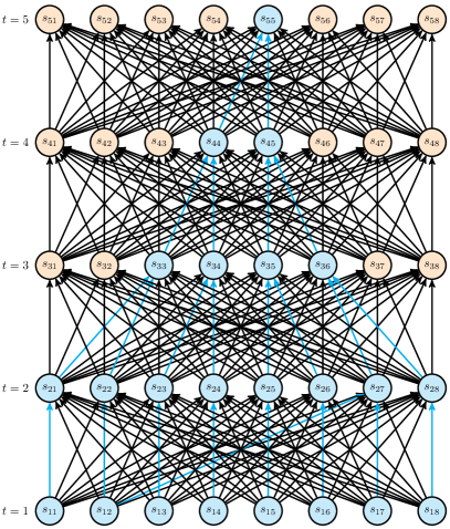
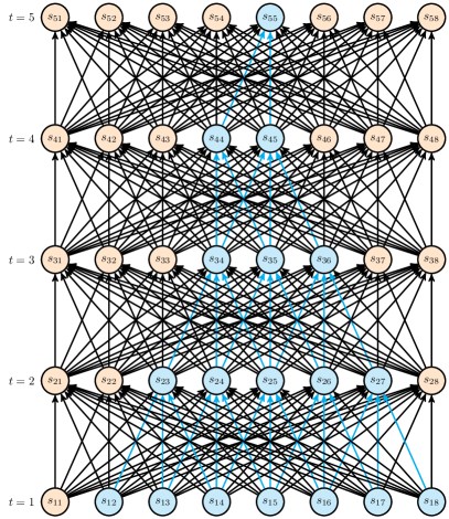
Figure A1: Examples of how affected states (cyan) affect states in a previous time step (indicated by cyan edges) starting with $n_{5}=1$ (one affected state). The left panel shows no overlap since affected states in $s_{t-1}$ connect only to one affected state in $s_{t}$. The right panel shows some overlap since affected states in $s_{t-1}$ connect to multiple affected states in $s_{t}$.

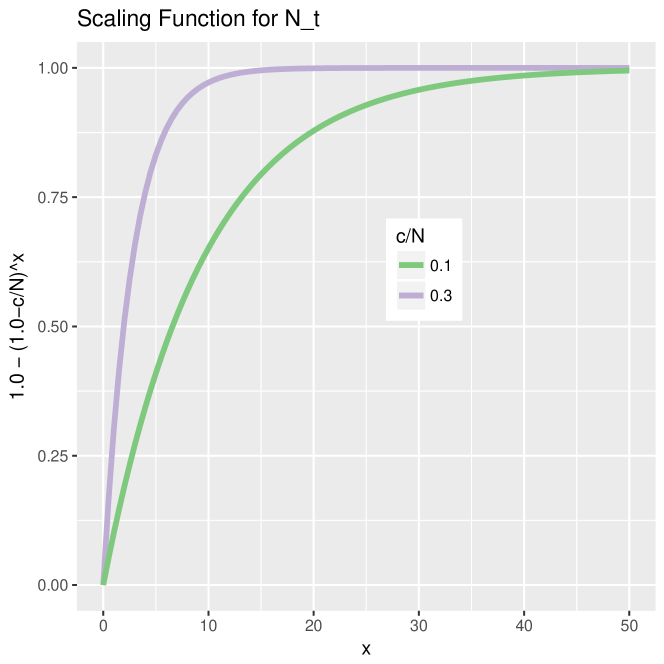
Figure A2: The function $\left(1-\left(1-\frac{c_{t}}{N_{t-1}}\right)^{n_{t}}\right)$ which scales $N_{t-1}$ in Theorem A10. This function determines the growth of $a_{k}$, which is exponentially at the beginning, and then linearly when the function approaches 1.

The next theorem states that the on-site variance $\bm{\omega}_{k}$ can have large effect on the variance of each previous state-action pair. Furthermore, for small $k$ the number of affected states grows exponentially, while for large $k$ it grows only linearly after some time $\hat{t}$. Figure A2 shows the function which determines how much $a_{k}$ grows with $k$.

Theorem A10.

For $t\leqslant k$, $\bm{\omega}_{k}$ contributes to $\bm{V}_{t}^{\pi}$ by the term $\bm{P}_{t\leftarrow k}\ \bm{\omega}_{k}$, where $\left\|\bm{P}_{t\leftarrow k}\right\|_{\infty}=1$.

The number $a_{k}$ of states affected by the on-site variance $\bm{\omega}_{k}$ is

$$a_{k}\ =\ \sum_{t=0}^{k}\left(1\ -\ \left(1\ -\ \frac{c_{t}}{N_{t-1}}\right)^{n_{t}}\right)\ N_{t-1}\ .$$ (A237)

Proof.

The “backward induction algorithm” [95, 96] gives with $\bm{V}_{T+1}^{\pi}=\bm{0}$ and on-site variance $\bm{\omega}_{T+1}=\bm{0}$:

$$\bm{V}_{t}^{\pi}\ =\ \sum_{k=t}^{T}\prod_{\tau=t}^{k-1}\bm{P}_{\tau}\ \bm{\omega}_{k}\ ,$$ (A238)

where we define $\prod_{\tau=t}^{t-1}\bm{P}_{\tau}=\bm{I}$ and $[\bm{\omega}_{k}]_{(s_{k},a_{k})}=\omega(s_{k},a_{k})$.

Since the product of two row-stochastic matrices is a row-stochastic matrix according to Lemma A4, $\bm{P}_{t\leftarrow k}=\prod_{\tau=t}^{k-1}\bm{P}_{\tau}$ is a row-stochastic matrix. Since $\left\|\bm{P}_{t\leftarrow k}\right\|_{\infty}=1$ according to Lemma A5, each on-site variance $\bm{\omega}_{k}$ with $t\leqslant k$ can have large effects on $\bm{V}_{t}^{\pi}$. Using the row-stochastic matrices $\bm{P}_{t\leftarrow k}$, we can reformulate the variance:

$$\bm{V}_{t}^{\pi}\ =\ \sum_{k=t}^{T}\bm{P}_{t\leftarrow k}\ \bm{\omega}_{k}\ ,$$ (A239)

with $\left\|\bm{P}_{t\leftarrow k}\right\|_{\infty}=1$. The on-site variance $\bm{\omega}_{k}$ at step $k$ increases all variances $\bm{V}_{t}^{\pi}$ with $t\leqslant k$.

Next we proof the second part of the theorem, which considers the growth of $a_{k}$. To compute $a_{k}$ we first have to know $n_{t}$. For computing $n_{t-1}$ from $n_{t}$, we want to know how many states are affected in $s_{t-1}$ if $n_{t}$ states are affected in $s_{t}$. The answer to this question is the expected coverage when searching a document collection using a set of independent computers [19]. We follow the approach of Cox et al. [19]. The minimal number of affected states in $s_{t-1}$ is $c_{t}$, where each of the $c_{t}$ affected states in $s_{t-1}$ connects to each of the $n_{t}$ states in $s_{t}$ (maximal overlap). The maximal number of affected states in $s_{t-1}$ is $c_{t}n_{t}$, where each affected state in $s_{t-1}$ connects to only one affected state in $s_{t}$ (no overlap). We consider a single state in $s_{t}$. The probability of a state in $s_{t-1}$ being connected to this single state in $s_{t}$ is $c_{t}/N_{t-1}$ and being not connected to this state in $s_{t}$ is $1-c_{t}/N_{t-1}$. The probability of a state in $s_{t-1}$ being not connected to any of the $n_{t}$ affected states in $s_{t}$ is

$$\left(1\ -\ \frac{c_{t}}{N_{t-1}}\right)^{n_{t}}\ .$$ (A240)

The probability of a state in $s_{t-1}$ being at least connected to one of the $n_{t}$ affected states in $s_{t}$ is

$$1\ -\ \left(1\ -\ \frac{c_{t}}{N_{t-1}}\right)^{n_{t}}\ .$$ (A241)

Thus, the expected number of distinct states in $s_{t-1}$ being connected to one of the $n_{t}$ affected states in $s_{t}$ is

$$n_{t-1}\ =\ \left(1\ -\ \left(1\ -\ \frac{c_{t}}{N_{t-1}}\right)^{n_{t}}\right)\ N_{t-1}\ .$$ (A242)

The number $a_{k}$ of affected states by $\bm{\omega}_{k}$ is

$$a_{k}\ =\ \sum_{t=0}^{k}\left(1\ -\ \left(1\ -\ \frac{c_{t}}{N_{t-1}}\right)^{n_{t}}\right)\ N_{t-1}\ .$$ (A243)

∎

Corollary A2.

For small $k$, the number $a_{k}$ of states affected by the on-site variance $\bm{\omega}_{k}$ at step $k$ grows exponentially with $k$ by a factor of $\bar{c}$:

$$a_{k}\ >\ \bar{c}^{k}\ .$$ (A244)

For large $k$ and after some time $t>\hat{t}$, the number $a_{k}$ of states affected by $\bm{\omega}_{k}$ grows linearly with $k$ with a factor of $\bar{N}$:

$$a_{k}\ \approx\ a_{\hat{t}-1}\ +\ (k-\hat{t}+1)\ \bar{N}\ .$$ (A245)

Proof.

For small $n_{t}$ with $\frac{c_{t}n_{t}}{N_{t-1}}\ll 1$, we have

$$\left(1\ -\ \frac{c_{t}}{N_{t-1}}\right)^{n_{t}}\ \approx\ 1\ -\ \frac{c_{t}\ n_{t}}{N_{t-1}}\ ,$$ (A246)

thus

$$n_{t-1}\ \approx\ c_{t}\ n_{t}\ .$$ (A247)

For large $N_{t-1}$ compared to the number of connections $c_{t}$ of a single state in $s_{t}$ to states in $s_{t-1}$, we have the approximation

$$\left(1\ -\ \frac{c_{t}}{N_{t-1}}\right)^{n_{t}}\ =\ \left(\left(1\ +\ \frac{-c_{t}}{N_{t-1}}\right)^{N_{t-1}}\right)^{n_{t}/N_{t-1}}\ \approx\ \exp(-(c_{t}\ n_{t})/N_{t-1})\ .$$ (A248)

We obtain

$$n_{t-1}\ =\ \left(1\ -\ \exp(-(c_{t}\ n_{t})/N_{t-1})\right)\ N_{t-1}\ .$$ (A249)

For small $n_{t}$, we again have

$$n_{t-1}\ \approx\ c_{t}\ n_{t}\ .$$ (A250)

Therefore, for small $k-t$, we obtain

$$n_{t}\ \approx\ \prod_{\tau=t}^{k}c_{\tau}\ \approx\ \bar{c}^{k-t}\ .$$ (A251)

Thus, for small $k$ the number $a_{k}$ of states affected by $\bm{\omega}_{k}$ is

$$a_{k}\ =\ \sum_{t=0}^{k}n_{t}\ \approx\ \sum_{t=0}^{k}\bar{c}^{k-t}\ =\ \sum_{t=0}^{k}\bar{c}^{t}\ =\ \frac{\bar{c}^{k+1}-1}{\bar{c}-1}\ >\ \bar{c}^{k}\ .$$ (A252)

Consequently, for small $k$ the number $a_{k}$ of states affected by $\bm{\omega}_{k}$ grows exponentially with $k$ by a factor of $\bar{c}$. For large $k$, at a certain time $t>\hat{t}$, $n_{t}$ has grown such that $c_{t}n_{t}>N_{t-1}$, yielding $\exp(-(c_{t}n_{t})/N_{t-1})\approx 0$, and thus

$$n_{t}\ \approx\ N_{t}\ .$$ (A253)

Therefore

$$a_{k}\ -\ a_{\hat{t}-1}\ =\ \sum_{t=\hat{t}}^{k}n_{t}\ \approx\ \sum_{t=\hat{t}}^{k}N_{t}\ \approx\ (k-\hat{t}+1)\ \bar{N}\ .$$ (A254)

Consequently, for large $k$ the number $a_{k}$ of states affected by $\bm{\omega}_{k}$ grows linearly with $k$ by a factor of $\bar{N}$. ∎

Therefore, we aim for decreasing the on-site variance $\bm{\omega}_{k}$ for large $k$, in order to reduce the variance. In particular, we want to avoid delayed rewards and provide the reward as soon as possible in each episode. Our goal is to give the reward as early as possible in each episode to reduce the variance of action-values that are affected by late rewards and their associated immediate and local variances.

Appendix A4 Experiments

A4.1 Artificial Tasks

This section provides more details for the artificial tasks (I), (II) and (III) in the main paper. Additionally, we include artificial task (IV) characterized by deterministic reward and state transitions, and artificial task (V) which is solved using policy gradient methods.

A4.1.1 Task (I): Grid World

This environment is characterized by probabilistic delayed rewards. It illustrates a situation, where a time bomb explodes at episode end. The agent has to defuse the bomb and then run away as far as possible since defusing fails with a certain probability. Alternatively, the agent can immediately run away, which, however, leads to less reward on average since the bomb always explodes. The Grid World is a quadratic $31\times 31$ grid with bomb at coordinate $[30,15]$ and start at $[30-d,15]$, where $d$ is the delay of the task. The agent can move in four different directions (up, right, left, and down). Only moves are allowed that keep the agent on the grid. The episode finishes after $1.5d$ steps. At the end of the episode, with a given probability of 0.5, the agent receives a reward of 1000 if it has visited bomb. At each time step the agent receives an immediate reward of $c\cdot t\cdot h$, where the factor $c$ depends on the chosen action, $t$ is the current time step, and $h$ is the Hamming distance to bomb. Each move of the agent, which reduces the Hamming distance to bomb, is penalized by the immediate reward via $c=-0.09$. Each move of the agent, which increases the Hamming distance to bomb, is rewarded by the immediate reward via $c=0.1$. The agent is forced to learn the $Q$-values precisely, since the immediate reward of directly running away hints at a sub-optimal policy.

For non-deterministic reward, the agent receives the delayed reward for having visited bomb with probability $p(r_{T+1}=100\mid s_{T},a_{T})$. For non-deterministic transitions, the probability of transiting to next state $s^{\prime}$ is $p(s^{\prime}\mid s,a)$. For the deterministic environment these probabilities were either 1 or zero.

Policy evaluation: learning the action-value estimator for a fixed policy.

First, the theoretical statements on bias and variance of estimating the action-values by TD in Theorem A8 and by MC in Theorem A10 are experimentally verified for a fixed policy. Secondly, we consider the bias and variance of TD and MC estimators of the transformed MDP with optimal reward redistribution according to Theorem A5.

The new MDP with an optimal reward redistribution has advantages over the original MDP both for TD and MC. For TD, the new MDP corrects the bias exponentially faster and for MC it has fewer number of action-values with high variance. Consequently, estimators for the new MDP learn faster than the same estimators in the original MDP.

Since the bias-variance analysis is defined for a particular number of samples drawn from a fixed distribution, we need to fix the policy for sampling. We use an $\epsilon$-greedy version of the optimal policy, where $\epsilon$ is chosen such that on average in 10% of the episodes the agent visits bomb. For the analysis, the delay ranges from 5 to 30 in steps of 5. The true $Q$-table for each delay is computed by backward induction and we use 10 different action-value estimators for computing bias and variance.

For the TD update rule we use the exponentially weighted arithmetic mean that is sample-updates, with initial value $q^{0}(s,a)=0$. We only monitor the mean and the variance for action-value estimators at the first time step, since we are interested in the time required for correcting the bias. 10 different estimators are run for 10,000 episodes. Figure 3(a) shows the bias correction for different delays, normalized by the first error.

For the MC update rule we use the arithmetic mean for policy evaluation (later we will use constant-$\alpha$ MC for learning the optimal policy). For each delay, a test set of state-actions for each delay is generated by drawing 5,000 episodes with the $\epsilon$-greedy optimal policy. For each action-value estimator the mean and the variance is monitored every 10 visits. If every action-value has 500 updates (visits), learning is stopped. Bias and variance are computed based on 10 different action-value estimators. As expected from Section A3.1, in Figure 3(b) the variance decreases by $1/n$, where $n$ is the number of samples. Figure 3(b) shows that the number of state-actions with a variance larger than a threshold increases exponentially with the delay. This confirms the statements of Theorem A10.

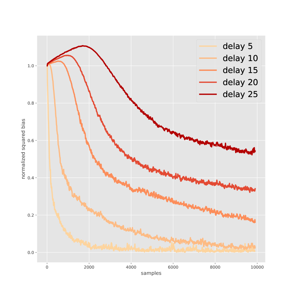
(a)

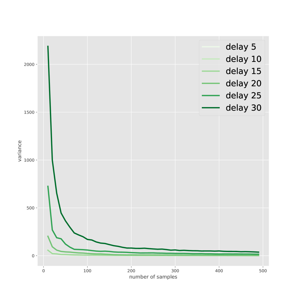
(b)

Figure A3: (a) Experimental evaluation of bias and variance of different $Q$-value estimators on the Grid World. (b) Normalized bias reduction for different delays. Right: Average variance reduction for the 10th highest values.

Learning the optimal policy.

For finding the optimal policy for the Grid World task, we apply Monte Carlo Tree Search (MCTS), $Q$-learning, and Monte Carlo (MC). We train until the greedy policy reaches 90% of the return of the optimal policy. The learning time is measured by the number of episodes. We use sample updates for $Q$-learning and MC [128]. For MCTS the greedy policy uses $0$ for the exploration constant in UCB1 [68]. The greedy policy is evaluated in 100 episodes intervals. The MCTS selection step begins in the start state, which is the root of the game tree that is traversed using UCB1 [68] as the tree policy. If a tree-node gets visited the first time, it is expanded with an initial value obtained by $100$ simulated trajectories that start at this node. These simulations use a uniform random policy whose average Return is calculated. The backpropagation step uses the MCTS(1) update rule [66]. The tree policies exploration constant is $\sqrt{2}$. $Q$-learning and MC use a learning rate of $0.3$ and an $\epsilon$-greedy policy with $\epsilon=0.3$. For RUDDER the optimal reward redistribution using a return decomposition as stated in Section A2.6.1 is used. For each delay and each method, 300 runs with different seeds are performed to obtain statistically relevant results.

Estimation of the median learning time and quantiles.

The performance of different methods is measured by the median learning time in terms of episodes. We stop training at $100$ million episodes. Some runs, especially for long delays, have taken too long and have thus been stopped. To resolve this bias the quantiles of the learning time are estimated by fitting a distribution using right censored data [33] .The median is still robustly estimated if more than 50% of runs have finished, which is the case for all plotted datapoints. We find that for delays where all runs have finished the learning time follows a Log-normal distribution. Therefore, we fit a Log-normal distribution on the right censored data. We estimate the median from the existing data, and use maximum likelihood estimation to obtain the second distribution parameter $\sigma^{2}$. The start value of the $\sigma^{2}$ estimation is calculated by the measured variance of the existing data which is algebraically transformed to get the $\sigma$ parameter.

A4.1.2 Task (II): The Choice

In this experiment we compare RUDDER, temporal difference (TD) and Monte Carlo (MC) in an environment with delayed deterministic reward and probabilistic state transitions to investigate how reward information is transferred back to early states. This environment is a variation of our introductory pocket watch example and reveals problems of TD and MC, while contribution analysis excels. In this environment, only the first action at the very beginning determines the reward at the end of the episode.

The environment

is an MDP consisting of two actions $a\in\mathcal{A}=\{+,-\}$, an initial state $s^{0}$, two charged states $s^{+}$, $s^{-}$, two neutral states $s^{\oplus}$, $s^{\ominus}$, and a final state $s^{\mathrm{f}}$. After the first action $a_{0}\in\mathcal{A}=\{+,-\}$ in state $s^{0}$, the agent transits to state $s^{+}$ for action $a_{0}=+$ and to $s^{-}$ for action $a_{0}=-$. Subsequent state transitions are probabilistic and independent on actions. With probability $p_{C}$ the agent stays in the charged states $s^{+}$ or $s^{-}$, and with probability $(1-p_{C})$ it transits from $s^{+}$ or $s^{-}$ to the neutral states $s^{\oplus}$ or $s^{\ominus}$, respectively. The probability to go from neutral states to charged states is $p_{C}$, and the probability to stay in neutral states is $(1-p_{C})$. Probabilities to transit from $s^{+}$ or $s^{\oplus}$ to $s^{-}$ or $s^{\ominus}$ or vice versa are zero. Thus, the first action determines whether that agent stays in "$+$"-states or "$-$"-states. The reward is determined by how many times the agent visits charged states plus a bonus reward depending on the agent’s first action. The accumulative reward is given at sequence end and is deterministic. After $T$ time steps, the agent is in the final state $s^{\mathrm{f}}$, in which the reward $R_{T+1}$ is provided. $R_{T+1}$ is the sum of 3 deterministic terms:

1. $R_{0}$, the baseline reward associated to the first action;

2. $R_{C}$, the collected reward across states, which depends on the number of visits $n$ to the charged states;

3. $R_{b}$, a bonus if the first action $a_{0}=+$.

The expectations of the accumulative rewards for $R_{0}$ and $R_{C}$ have the same absolute value but opposite signs, therefore they cancel in expectation over episodes. Thus, the expected return of an episode is the expected reward $R_{b}$: $p(a_{0}=+)b$. The rewards are defined as follows:

$$c_{0}\ =\ \begin{cases}~{}~{}~{}1&\text{if }\ a_{0}=+\\ -1&\text{if }\ a_{0}=-\ ,\end{cases}$$ (A255)

$$R_{b}\ =\ \begin{cases}b&\text{if }\ a_{0}=+\\ 0&\text{if }\ a_{0}=-\ ,\end{cases}$$ (A256)

$$R_{C}\ =\ c_{0}\ C\ n\ ,$$ (A257)

$$R_{0}\ =\ -\ c_{0}\ C\ p_{C}\ T\ ,$$ (A258)

$$R_{T+1}\ =\ R_{C}\ +\ R_{0}\ +\ R_{b}\ ,$$ (A259)

where $C$ is the baseline reward for charged states, and $p_{C}$ the probability of staying in or transiting to charged states. The expected visits of charged states is $\mathbf{\mathrm{E}}[n]=p_{C}T$ and $\mathbf{\mathrm{E}}[R_{T+1}]=\mathbf{\mathrm{E}}[R_{b}]=p(a_{0}=+)b$.

Figure A4: State transition diagram for The Choice task. The diagram is a simplification of the actual MDP.

Methods compared:

The following methods are compared:

1. $Q$-learning with eligibility traces according to Watkins [140],

2. Monte Carlo,

3. RUDDER with reward redistribution.

For RUDDER, we use an LSTM without lessons buffer and without safe exploration. Contribution analysis is realized by differences of return predictions. For MC, $Q$-values are the exponential moving average of the episode return. For RUDDER, the $Q$-values are estimated by an exponential moving average of the reward redistribution.

Performance evaluation and results.

The task is considered as solved when the exponential moving average of the selection of the desired action at time $t=0$ is equal to $1-\epsilon$, where $\epsilon$ is the exploration rate. The performances of the compared methods are measured by the average learning time in the number of episodes required to solve the task. A Wilcoxon signed-rank test is performed between the learning time of RUDDER and those of the other methods. Statistical significance p-values are obtained by Wilcoxon signed-rank test. RUDDER with reward redistribution is significantly faster than all other methods with p-values $<10^{-8}$. Table A1 reports the number of episodes required by different methods to solve the task. RUDDER with reward redistribution clearly outperforms all other methods.

Table A1: Number of episodes required by different methods to solve the grid world task with delayed reward. Numbers give the mean and the standard deviation over 100 trials. RUDDER with reward redistribution clearly outperforms all other TD methods.

Method	Delay 10			Delay 15			Delay 20
RUDDER	3520.06	$\pm$ 2343.79	p = 5.00E-01	3062.07	$\pm$ 1278.92	p = 5.00E-01	3813.96	$\pm$ 2738.18	p = 5.00E-01
MC	10920.64	$\pm$ 7550.04	p = 5.03E-24	17102.89	$\pm$ 12640.09	p = 1.98E-30	22910.85	$\pm$ 19149.02	p = 1.25E-28
Q	66140.76	$\pm$ 1455.33	p = 1.28E-34	115352.25	$\pm$ 1962.20	p = 1.28E-34	171571.94	$\pm$ 2436.25	p = 1.28E-34

Method	Delay 25			Delay 30			Delay 35
MC	39772	$\pm$ 47460	p < 1E-29	41922	$\pm$ 36618	p < 1E-30	50464	$\pm$ 60318	p < 1E-30
Q	234912	$\pm$ 2673	p < 1E-33	305894	$\pm$ 2928	p < 1E-33	383422	$\pm$ 4346	p < 1E-22
RUDDER	4112	$\pm$ 3769		3667	$\pm$ 1776		3850	$\pm$ 2875

Method	Delay 40			Delay 45			Delay 50
MC	56945	$\pm$ 54150	p < 1E-30	69845	$\pm$ 79705	p < 1E-31	73243	$\pm$ 70399	p = 1E-31
Q	466531	$\pm$ 3515	p = 1E-22
RUDDER	3739	$\pm$ 2139		4151	$\pm$ 2583		3884	$\pm$ 2188

Method	Delay 100			Delay 500
MC	119568	$\pm$ 110049	p < 1E-11	345533	$\pm$ 320232	p < 1E-16
RUDDER	4147	$\pm$ 2392		5769	$\pm$ 4309

A4.1.3 Task(III): Trace-Back

This section supports the artificial task (III) – Trace-Back – in the main paper. RUDDER is compared to potential-based reward shaping methods. In this experiment, we compare reinforcement learning methods that have to transfer back information about a delayed reward. These methods comprise RUDDER, TD($\lambda$) and potential-based reward shaping approaches. For potential-based reward shaping we compare the original reward shaping [87], look-forward advice, and look-back advice [143] with three different potential functions. Methods that transfer back reward information are characterized by low variance estimates of the value function or the action-value function, since they use an estimate of the future return instead of the future return itself. To update the estimates of the future returns, reward information has to be transferred back. The task in this experiment can be solved by Monte Carlo estimates very fast, which do not transfer back information but use samples of the future return for the estimation instead. However, Monte Carlo methods have high variance, which is not considered in this experiment.

The environment

is a 15$\times$15 grid, where actions move the agent from its current position in 4 adjacent positions (up, down, left, right), except the agent would be moved outside the grid. The number of steps (moves) per episode is $T=20$. The starting position is $(7,7)$ in the middle of the grid. The maximal return is a combination of negative immediate reward and positive delayed reward. To obtain the maximum return, the policy must move the agent up in the time step $t=1$ and right in the following time step $t=2$. In this case, the agent receives an immediate reward of -50 at $t=2$ and a delayed reward of 150 at the end of the episode at $t=20$, that is, a return of 100. Any other combination of actions gives the agent immediate reward of 50 at $t=2$ without any delayed reward, that is, a return of 50. To ensure Markov properties the position of the agent, the time, as well as the delayed reward are coded in the state. The future reward discount rate $\gamma$ is set to 1. The state transition probabilities are deterministic for the first two moves. For $t>2$ and for each action, state transition probabilities are equal for each possible next state (uniform distribution), meaning that actions after $t=2$ do not influence the return. For comparisons of long delays, both the size of the grid and the length of the episode are increased. For a delay of $n$, a $(3n/4)\times(3n/4)$ grid is used with an episode length of $n$, and starting position $(3n/8,3n/8)$.

Compared methods.

We compare different TD($\lambda$) and potential-based reward shaping methods. For TD($\lambda$), the baseline is $Q(\lambda)$, with eligibility traces $\lambda=0.9$ and $\lambda=0$ and Watkins’ implementation [140]. The potential-based reward shaping methods are the original reward shaping, look-ahead advice as well as look-back advice. For look-back advice, we use SARSA($\lambda$) [105] instead of $Q(\lambda)$ as suggested by the authors [143]. $Q$-values are represented by a state-action table, that is, we consider only tabular methods. In all experiments an $\epsilon$-greedy policy with $\epsilon=0.2$ is used. All three reward shaping methods require a potential function $\phi$, which is based on the reward redistribution ($\tilde{r}_{t}$) in three different ways:

(I) The Potential function $\phi$ is the difference of LSTM predictions, which is the redistributed reward $R_{t}$:

$$\phi(s_{t})\ =\ \mathbf{\mathrm{E}}\left[R_{t+1}\mid s_{t}\right]\ \ \mbox{ or }$$ (A260)

$$\phi(s_{t},a_{t})\ =\ \mathbf{\mathrm{E}}\left[R_{t+1}\mid s_{t},a_{t}\right]\ .$$ (A261)

(II) The potential function $\phi$ is the sum of future redistributed rewards, i.e. the q-value of the redistributed rewards. In the optimal case, this coincides with implementation (I):

$$\phi(s_{t})\ =\ \mathbf{\mathrm{E}}\left[\sum^{T}_{\tau=t}R_{\tau+1}\mid s_{t}\right]\ \ \mbox{ or }$$ (A262)

$$\phi(s_{t},a_{t})\ =\ \mathbf{\mathrm{E}}\left[\sum^{T}_{\tau=t}R_{\tau+1}\mid s_{t},a_{t}\right]\ .$$ (A263)

(III) The potential function $\phi$ corresponds to the LSTM predictions. In the optimal case this corresponds to the accumulated reward up to $t$ plus the q-value of the delayed MDP:

$$\phi(s_{t})\ =\ \mathbf{\mathrm{E}}\left[\sum^{T}_{\tau=0}\tilde{R}_{\tau+1}\mid s_{t}\right]\ \ \mbox{ or }$$ (A264)

$$\phi(s_{t},a_{t})\ =\ \mathbf{\mathrm{E}}\left[\sum^{T}_{\tau=0}\tilde{R}_{\tau+1}\mid s_{t},a_{t}\right]\ .$$ (A265)

The following methods are compared:

1. $Q$-learning with eligibility traces according to Watkins ($Q(\lambda)$),

2. SARSA with eligibility traces (SARSA($\lambda$)),

3. Reward Shaping with potential functions (I), (II), or (III) according to $Q$-learning and eligibility traces according to Watkins,

4. Look-ahead advise with potential functions (I), (II), or (III) with $Q(\lambda)$,

5. Look-back advise with potential functions (I), (II), or (III) with SARSA($\lambda$),

6. RUDDER with reward redistribution for $Q$-value estimation and RUDDER applied on top of $Q$-learning.

RUDDER is implemented with an LSTM architecture without output gate nor forget gate. For this experiments, RUDDER does not use lessons buffer nor safe exploration. For contribution analysis we use differences of return predictions. For RUDDER, the $Q$-values are estimated by an exponential moving average (RUDDER $Q$-value estimation) or alternatively by $Q$-learning.

Performance evaluation:

The task is considered solved when the exponential moving average of the return is above 90, which is 90% of the maximum return. Learning time is the number of episodes required to solve the task. The first evaluation criterion is the average learning time. The $Q$-value differences at time step $t=2$ are monitored. The $Q$-values at $t=2$ are the most important ones, since they have to predict whether the maximal return will be received or not. At $t=2$ the immediate reward acts as a distraction since it is -50 for the action leading to the maximal return ($a^{+}$) and 50 for all other actions ($a^{-}$). At the beginning of learning, the $Q$-value difference between $a^{+}$ and $a^{-}$ is about -100, since the immediate reward is -50 and 50, respectively. Once the $Q$-values converge to the optimal policy, the difference approaches 50. However, the task will already be correctly solved as soon as this difference is positive. The second evaluation criterion is the $Q$-value differences at time step $t=2$, since it directly shows to what extend the task is solved.

Results:

Table A1 reports the number of episodes required by different methods to solve the task. The mean and the standard deviation over 100 trials are given. A Wilcoxon signed-rank test is performed between the learning time of RUDDER and those of the other methods. Statistical significance p-values are obtained by Wilcoxon signed-rank test. RUDDER with reward redistribution is significantly faster than all other methods with p-values $<10^{-17}$. Tables A2,A3 report the results for all methods.

Table A2: Number of episodes required by different methods to solve the Trace-Back task with delayed reward. The numbers represent the mean and the standard deviation over 100 trials. RUDDER with reward redistribution significantly outperforms all other methods.

Method	Delay 6			Delay 8			Delay 10
Look-back I	6074	$\pm$ 952	p = 1E-22	13112	$\pm$ 2024	p = 1E-22	21715	$\pm$ 4323	p = 1E-06
Look-back II	4584	$\pm$ 917	p = 1E-22	9897	$\pm$ 2083	p = 1E-22	15973	$\pm$ 4354	p = 1E-06
Look-back III	4036.48	$\pm$ 1424.99	p = 5.28E-17	7812.72	$\pm$ 2279.26	p = 1.09E-23	10982.40	$\pm$ 2971.65	p = 1.03E-07
Look-ahead I	14469.10	$\pm$ 1520.81	p = 1.09E-23	28559.32	$\pm$ 2104.91	p = 1.09E-23	46650.20	$\pm$ 3035.78	p = 1.03E-07
Look-ahead II	12623.42	$\pm$ 1075.25	p = 1.09E-23	24811.62	$\pm$ 1986.30	p = 1.09E-23	43089.00	$\pm$ 2511.18	p = 1.03E-07
Look-ahead III	16050.30	$\pm$ 1339.69	p = 1.09E-23	30732.00	$\pm$ 1871.07	p = 1.09E-23	50340.00	$\pm$ 2102.78	p = 1.03E-07
Reward Shaping I	14686.12	$\pm$ 1645.02	p = 1.09E-23	28223.94	$\pm$ 3012.81	p = 1.09E-23	46706.50	$\pm$ 3649.57	p = 1.03E-07
Reward Shaping II	11397.10	$\pm$ 905.59	p = 1.09E-23	21520.98	$\pm$ 2209.63	p = 1.09E-23	37033.40	$\pm$ 1632.24	p = 1.03E-07
Reward Shaping III	12125.48	$\pm$ 1209.59	p = 1.09E-23	23680.98	$\pm$ 1994.07	p = 1.09E-23	40828.70	$\pm$ 2748.82	p = 1.03E-07
$Q(\lambda)$	14719.58	$\pm$ 1728.19	p = 1.09E-23	28518.70	$\pm$ 2148.01	p = 1.09E-23	44017.20	$\pm$ 3170.08	p = 1.03E-07
SARSA($\lambda$)	8681.94	$\pm$ 704.02	p = 1.09E-23	23790.40	$\pm$ 836.13	p = 1.09E-23	48157.50	$\pm$ 1378.38	p = 1.03E-07
RUDDER $Q(\lambda)$	726.72	$\pm$ 399.58	p = 3.49E-04	809.86	$\pm$ 472.27	p = 3.49E-04	906.13	$\pm$ 514.55	p = 3.36E-02
RUDDER	995.59	$\pm$ 670.31	p = 5.00E-01	1128.82	$\pm$ 741.29	p = 5.00E-01	1186.34	$\pm$ 870.02	p = 5.00E-01

Method	Delay 12			Delay 15			Delay 17
Look-back I	33082.56	$\pm$ 7641.57	p = 1.09E-23	49658.86	$\pm$ 8297.85	p = 1.28E-34	72115.16	$\pm$ 21221.78	p = 1.09E-23
Look-back II	23240.16	$\pm$ 9060.15	p = 1.09E-23	29293.94	$\pm$ 7468.94	p = 1.28E-34	42639.38	$\pm$ 17178.81	p = 1.09E-23
Look-back III	15647.40	$\pm$ 4123.20	p = 1.09E-23	20478.06	$\pm$ 5114.44	p = 1.28E-34	26946.92	$\pm$ 10360.21	p = 1.09E-23
Look-ahead I	66769.02	$\pm$ 4333.47	p = 1.09E-23	105336.74	$\pm$ 4977.84	p = 1.28E-34	136660.12	$\pm$ 5688.32	p = 1.09E-23
Look-ahead II	62220.56	$\pm$ 3139.87	p = 1.09E-23	100505.05	$\pm$ 4987.16	p = 1.28E-34	130271.88	$\pm$ 5397.61	p = 1.09E-23
Look-ahead III	72804.44	$\pm$ 4232.40	p = 1.09E-23	115616.59	$\pm$ 5648.99	p = 1.28E-34	149064.68	$\pm$ 7895.48	p = 1.09E-23
Reward Shaping I	68428.04	$\pm$ 3416.12	p = 1.09E-23	107399.17	$\pm$ 5242.88	p = 1.28E-34	137032.14	$\pm$ 6663.12	p = 1.09E-23
Reward Shaping II	56225.24	$\pm$ 3778.86	p = 1.09E-23	93091.44	$\pm$ 5233.02	p = 1.28E-34	122224.20	$\pm$ 5545.63	p = 1.09E-23
Reward Shaping III	60071.52	$\pm$ 3809.29	p = 1.09E-23	99476.40	$\pm$ 5607.08	p = 1.28E-34	130103.50	$\pm$ 6005.61	p = 1.09E-23
$Q(\lambda)$	66952.16	$\pm$ 4137.67	p = 1.09E-23	107438.36	$\pm$ 5327.95	p = 1.28E-34	135601.26	$\pm$ 6385.76	p = 1.09E-23
SARSA($\lambda$)	78306.28	$\pm$ 1813.31	p = 1.09E-23	137561.92	$\pm$ 2350.84	p = 1.28E-34	186679.12	$\pm$ 3146.78	p = 1.09E-23
RUDDER $Q(\lambda)$	1065.16	$\pm$ 661.71	p = 3.19E-01	972.73	$\pm$ 702.92	p = 1.13E-04	1101.24	$\pm$ 765.76	p = 1.54E-01
RUDDER	1121.70	$\pm$ 884.35	p = 5.00E-01	1503.08	$\pm$ 1157.04	p = 5.00E-01	1242.88	$\pm$ 1045.15	p = 5.00E-01

Table A3: Cont. Number of episodes required by different methods to solve the Trace-Back task with delayed reward. The numbers represent the mean and the standard deviation over 100 trials. RUDDER with reward redistribution significantly outperforms all other methods.

Method	Delay 20			Delay 25
Look-back I	113873.30	$\pm$ 31879.20	p = 1.03E-07
Look-back II	56830.30	$\pm$ 19240.04	p = 1.03E-07	111693.34	$\pm$ 73891.21	p = 1.09E-23
Look-back III	35852.10	$\pm$ 11193.80	p = 1.03E-07
Look-ahead I	187486.50	$\pm$ 5142.87	p = 1.03E-07
Look-ahead II	181974.30	$\pm$ 5655.07	p = 1.03E-07	289782.08	$\pm$ 11984.94	p = 1.09E-23
Look-ahead III	210029.90	$\pm$ 6589.12	p = 1.03E-07
Reward Shaping I	189870.30	$\pm$ 7635.62	p = 1.03E-07	297993.28	$\pm$ 9592.30	p = 1.09E-23
Reward Shaping II	170455.30	$\pm$ 6004.24	p = 1.03E-07	274312.10	$\pm$ 8736.80	p = 1.09E-23
Reward Shaping III	183592.60	$\pm$ 6882.93	p = 1.03E-07	291810.28	$\pm$ 10114.97	p = 1.09E-23
$Q(\lambda)$	186874.40	$\pm$ 7961.62	p = 1.03E-07
SARSA($\lambda$)	273060.70	$\pm$ 5458.42	p = 1.03E-07	454031.36	$\pm$ 5258.87	p = 1.09E-23
RUDDER I	1048.97	$\pm$ 838.26	p = 5.00E-01	1236.57	$\pm$ 1370.40	p = 5.00E-01
RUDDER II	1159.30	$\pm$ 731.46	p = 8.60E-02	1195.75	$\pm$ 859.34	p = 4.48E-01

A4.1.4 Task (IV): Charge-Discharge

The Charge-Discharge task depicted in Figure A5 is characterized by deterministic reward and state transitions. The environment consists of two states: charged $\mathtt{C}$ / discharged $\mathtt{D}$ and two actions charge $\mathtt{c}$ / discharge $\mathtt{d}$. The deterministic reward is $r(\mathtt{D},\mathtt{d})=1,r(\mathtt{C},\mathtt{d})=10,r(\mathtt{D},\mathtt{c})=0$, and $r(\mathtt{C},\mathtt{c})=0$. The reward $r(\mathtt{C},\mathtt{d})$ is accumulated for the whole episode and given only at time $T+1$, where $T$ corresponds to the maximal delay of the reward. The optimal policy alternates between charging and discharging to accumulate a reward of 10 every other time step. The smaller immediate reward of $1$ distracts the agent from the larger delayed reward. The distraction forces the agent to learn the value function well enough to distinguish between the contribution of the immediate and the delayed reward to the final return.

Figure A5: The Charge-Discharge task with two basic states: charged $\mathtt{C}$ and discharged $\mathtt{D}$. In each state the actions charge $\mathtt{c}$ leading to the charged state $\mathtt{C}$ and discharge $\mathtt{d}$ leading to discharged state $\mathtt{D}$ are possible. Action $\mathtt{d}$ in the discharged state $\mathtt{D}$ leads to a small immediate reward of $1$ and in the charged state $\mathtt{C}$ to a delayed reward of $10$. After sequence end $T=4$, the accumulated delayed reward $r_{T+1}=r_{5}$ is given.

For this task, the RUDDER backward analysis is based on monotonic LSTMs and on layer-wise relevance propagation (LRP). The reward redistribution provided by RUDDER uses an LSTM which consists of $5$ memory cells and is trained with Adam and a learning rate of $0.01$. The reward redistribution is used to learn an optimal policy by $Q$-learning and by MC with a learning rate of $0.1$ and an exploration rate of $0.1$. Again, we use sample updates for $Q$-learning and MC [128]. The learning is stopped either if the agent achieves $90$% of the reward of the optimal policy or after a maximum number of $10$ million episodes. For each $T$ and each method, 100 runs with different seeds are performed to obtain statistically relevant results. For delays with runs which did not finish within 100m episodes we estimate parameters like described in Paragraph A4.1.1.

A4.1.5 Task (V): Solving Trace-Back using policy gradient methods

In this experiment, we compare policy gradient methods instead of $Q$-learning based methods. These methods comprise RUDDER on top of PPO with and without GAE, and a baseline PPO using GAE. The environment and performance evaluation are the same as reported in Task III. Again, RUDDER is exponentially faster than PPO. RUDDER on top of PPO is slightly better with GAE than without.

Figure A6: Comparison of performance of RUDDER with GAE (RUDDER+GAE) and without GAE (RUDDER) and PPO with GAE (PPO) on artificial task V with respect to the learning time in episodes (median of 100 trials) in log scale vs. the delay of the reward. The shadow bands indicate the $40\%$ and $60\%$ quantiles. Again, RUDDER significantly outperforms all other methods.

A4.2 Atari Games

In this section we describe the implementation of RUDDER for Atari games. The implementation is largely based on the OpenAI baselines package [21] for the RL components and our package for the LSTM reward redistribution model, which will be announced upon publication. If not specified otherwise, standard input processing, such as skipping $3$ frames and stacking $4$ frames, is performed by the OpenAI baselines package.

We consider the 52 Atari games that were compatible with OpenAI baselines, Arcade Learning Environment (ALE) [11], and OpenAI Gym [18]. Games are divided into episodes, i.e. the loss of a life or the exceeding of 108k frames trigger the start of a new episode without resetting the environment. Source code will be made available at upon publication.

A4.2.1 Architecture

We use a modified PPO architecture and a separate reward redistribution model. While parts of the two could be combined, this separation allows for better comparison between the PPO baseline with and without RUDDER.

PPO architecture.

The design of the policy and the value network relies on the ppo2 implementation [21], which is depicted in Figure A7 and summarized in Table A4. The network input, 4 stacked Atari game frames [82], is processed by 3 convolution layers with ReLU activation functions, followed by a fully connected layer with ReLU activation functions. For PPO with RUDDER, 2 output units, for the original and redistributed reward value function, and another set of output units for the policy prediction are applied. For the PPO baseline without RUDDER, the output unit for the redistributed reward value function is omitted.

Reward redistribution model.

Core of the reward redistribution model is an LSTM layer containing 64 memory cells with sigmoid gate activations, tanh input nonlinearities, and identity output activation functions, as illustrated in Figure A7 and summarized in Table A4. This LSTM implementation omits output gate and forget gate to simplify the network dynamics. Identity output activation functions were chosen to support the development of linear counting dynamics within the LSTM layer, as is required to count the reward pieces during an episode chunk. Furthermore, the input gate is only connected recurrently to other LSTM blocks and the cell input is only connected to forward connections from the lower layer. For the vision system the same architecture was used as with the PPO network, with the first convolution layer being doubled to process $\Delta$ frames and full frames separately in the first layer. Additionally, the memory cell layer receives the vision feature activations of the PPO network, the current action, and the approximate in-game time as inputs. No gradients from the reward redistribution network are propagated over the connections to the PPO network. After the LSTM layer, the reward redistribution model has one output node for the prediction $\widehat{\mathbf{g}}$ of the return realization $\mathbf{g}$ of the return variable $G_{0}$. The reward redistribution model has 4 additional output nodes for the auxiliary tasks as described in Section A4.2.3.

Figure A7: RUDDER architecture for Atari games as described in Section A4.2.1. Left: The ppo2 implementation [21]. Right: LSTM reward redistribution architecture. The reward redistribution network has access to the PPO vision features (dashed lines) but no gradient is propagated between the networks. The LSTM layer receives the current action and an approximate in-game-time as additional input. The PPO outputs $v$ for value function prediction and $\pi$ for policy prediction each represent multiple output nodes: the original and redistributed reward value function prediction for $v$ and the outputs for all of the available actions for $\pi$. Likewise, the reward redistribution network output $\widehat{\mathbf{g}}$ represents multiple outputs, as described in Section A4.2.3 Details on layer configuration are given in Table A4.

Layer	Specifications		Layer	Specifications
Conv.Layer 0	features	32	Conv.Layer 4	features	32
	kernelsize	8x8		kernelsize	8x8
	striding	4x4		striding	4x4
	act	ReLU		act	ReLU
	initialization	orthogonal, gain=$\sqrt{2}$		initialization	orthogonal, gain=$0.1$
Conv.Layer 1	features	64	Conv.Layer 5	features	64
	kernelsize	4x4		kernelsize	4x4
	striding	2x2		striding	2x2
	act	ReLU		act	ReLU
	initialization	orthogonal, gain=$\sqrt{2}$		initialization	orthogonal, gain=$0.1$
Conv.Layer 2	features	64	Conv.Layer 6	features	64
	kernelsize	3x3		kernelsize	3x3
	striding	1x1		striding	1x1
	act	ReLU		act	ReLU
	initialization	orthogonal, gain=$\sqrt{2}$		initialization	orthogonal, gain=$0.1$
Dense Layer	features	512	LSTM Layer	cells	64
	act	ReLU		gate act.	sigmoid
	initialization	orthogonal, gain=$\sqrt{2}$		ci act.	tanh
Conv.Layer 3	features	32		output act.	linear
	kernelsize	8x8		bias ig	trunc.norm., mean$=-5$
	striding	4x4		bias ci	trunc.norm., mean$=0$
	act	ReLU		fwd.w. ci	trunc.norm., scale$=0.0001$
	initialization	orthogonal, gain=$0.1$		fwd.w. ig	omitted
				rec.w. ci	omitted
				rec.w. ig	trunc.norm., scale$=0.001$
				og	omitted
				fg	omitted

Table A4: Specifications of PPO and RUDDER architectures as shown in Figure A7. Truncated normal initialization has the default values mean$=0$, stddev$=1$ and is optionally multiplied by a factor scale.

A4.2.2 Lessons Replay Buffer

The lessons replay buffer is realized as a priority-based buffer containing up to $128$ samples. New samples are added to the buffer if (i) the buffer is not filled or if (ii) the new sample is considered more important than the least important sample in the buffer, in which case the new sample replaces the least important sample.

Importance of samples for the buffer is determined based on a combined ranking of (i) the reward redistribution model error and (ii) the difference of the sample return to the mean return of all samples in the lessons buffer. Each of these two rankings contributes equally to the final ranking of the sample. Samples with higher loss and greater difference to the mean return achieve a higher ranking.

Sampling from the lessons buffer is performed as a sampling from a softmax function on the sample-losses in the buffer. Each sample is a sequence of $512$ consecutive transitions, as described in the last paragraph of Section A4.2.3.

A4.2.3 Game Processing, Update Design, and Target Design

Reward redistribution is performed in an online fashion as new transitions are sampled from the environment. This allows to keep the original update schema of the PPO baseline, while still using the redistributed reward for the PPO updates. Training of the reward redistribution model is done separately on the lessons buffer samples from Section A4.2.2. These processes are described in more detail in the following paragraphs.

Reward Scaling.

As described in the main paper, rewards for the PPO baseline and RUDDER are scaled based on the maximum return per sample encountered during training so far. With $i$ samples sampled from the environment and a maximum return of $\mathbf{g}_{i}^{\max}=\max_{1\leqslant j\leqslant i}\{{{\left|\mathbf{g}_{j}\right|}}\}$ encountered, the scaled reward $r_{\mathrm{new}}$ is

$$r_{\mathrm{new}}\ =\ \frac{10\ r}{\mathbf{g}_{i}^{\max}}\ .$$ (A266)

Goal of this scaling is to normalize the reward $r$ to range $[-10,10]$ with a linear scaling, suitable for training the PPO and reward redistribution model. Since the scaling is linear, the original proportions between rewards are kept. Downside to this approach is that if a new maximum return is encountered, the scaling factor is updated, and the models have to readjust.

Reward redistribution.

Reward redistribution is performed using differences of return predictions of the LSTM network. That is, the differences of the reward redistribution model prediction $\widehat{\mathbf{g}}$ at time step $t$ and $t-1$ serve as contribution analysis and thereby give the redistributed reward $r_{t}=\widehat{\mathbf{g}}_{t}-\widehat{\mathbf{g}}_{t-1}$. This allows for online reward redistribution on the sampled transitions before they are used to train the PPO network, without waiting for the game sequences to be completed.

To assess the current quality of the reward redistribution model, a quality measure based on the relative absolute error of the prediction $\widehat{\mathbf{g}}_{T}$ at the last time step $T$ is introduced:

quality $$=\ 1\ -\ \frac{{{\left|\mathbf{g}-\widehat{\mathbf{g}}_{T}\right|}}}{\mu}\ \frac{1}{1-\epsilon},$$ (A267)

with $\epsilon$ as quality threshold of $\epsilon=80\%$ and the maximum possible error $\mu$ as $\mu=10$ due to the reward scaling applied. quality is furthermore clipped to be within range $[0,1]$.

PPO model.

The ppo2 implementation [21] samples from the environment using multiple agents in parallel. These agents play individual environments but share all weights, i.e. they are distinguished by random effects in the environment or by exploration. The value function and policy network is trained online on a batch of transitions sampled from the environment. Originally, the policy/value function network updates are adjusted using a policy loss, a value function loss, and an entropy term, each with dedicated scaling factors [115]. To decrease the number of hyperparameters, the entropy term scaling factor is adjusted automatically using Proportional Control to keep the policy entropy in a predefined range.

We use two value function output units to predict the value functions of the original and the redistributed reward. For the PPO baseline without RUDDER, the output unit for the redistributed reward is omitted. Analogous to the ppo2 implementation, these two value function predictions serve to compute the advantages used to scale the policy gradient updates. For this, the advantages for original reward $a_{o}$ and redistributed reward $a_{r}$ are combined as a weighted sum $a=a_{o}\ (1-\text{\tt qualityv})+a_{r}\ \text{\tt quality}$. The PPO value function loss term $L_{v}$ is replaced by the sum of the value function $v_{o}$ loss $L_{o}$ for the original reward and the scaled value function $v_{r}$ loss $L_{r}$ for the redistributed reward, such that $L_{v}=L_{o}+L_{r}\ \text{\tt quality}$. Parameter values were taken from the original paper [115] and implementation [21]. Additionally, a coarse hyperparameter search was performed with value function coefficients $\{0.1,1,10\}$ and replacing the static entropy coefficient by a Proportional Control scaling of the entropy coefficient. The Proportional Control target entropy was linearly decreased from $1$ to $0$ over the course of training. PPO baseline hyperparamters were used for PPO with RUDDER without changes.

Parameter values are listed in Table A5.

Reward redistribution model.

The loss of the reward redistribution model for a sample is composed of four parts. (i) The main loss $L_{m}$, which is the squared prediction loss of $\mathbf{g}$ at the last time step $T$ of the episode

$$L_{m}\ =\ \left(\mathbf{g}\ -\ \widehat{\mathbf{g}}_{T}\right)^{2}\ ,$$ (A268)

(ii) the continuous prediction loss $L_{c}$ of $\mathbf{g}$ at each time step

$$L_{c}\ =\ \frac{1}{T+1}\ \sum_{t=0}^{T}\left(\mathbf{g}´\ -\ \widehat{\mathbf{g}}_{t}\right)^{2}\ ,$$ (A269)

(iii) the loss $L_{e}$ of the prediction of the output at $t+10$ at each time step $t$

$$L_{e}\ =\ \frac{1}{T-9}\ \sum_{t=0}^{T-10}\left(\widehat{\mathbf{g}}_{t+10}\ -\ \widehat{\left(\widehat{\mathbf{g}}_{t+10}\right)}_{t}\right)^{2}\ ,$$ (A270)

as well as (iv) the loss on 3 auxiliary tasks. At every time step $t$, these auxiliary tasks are (1) the prediction of the action-value function $\widehat{q}_{t}$, (2) the prediction of the accumulated original reward $\tilde{r}$ in the next 10 frames $\sum_{i=t}^{t+10}\tilde{r}_{i}$, and (3) the prediction of the accumulated reward in the next 50 frames $\sum_{i=t}^{t+50}\tilde{r}_{i}$, resulting in the final auxiliary loss $L_{a}$ as

$$L_{a1}\ =\ \frac{1}{T+1}\ \sum_{t=0}^{T}\left(q_{t}\ -\ \widehat{q}_{t}\right)^{2}\ ,$$ (A271)

$$L_{a2}\ =\ \frac{1}{T-9}\ \sum_{t=0}^{T-10}\left(\sum_{i=t}^{t+10}\tilde{r}_{i}\ -\ \widehat{\left(\sum_{i=t}^{t+10}\tilde{r}_{i}\right)}_{t}\right)^{2}\ ,$$ (A272)

$$L_{a3}\ =\ \frac{1}{T-49}\ \sum_{t=0}^{T-50}\left(\sum_{i=t}^{t+50}\tilde{r}_{i}\ -\ \widehat{\left(\sum_{i=t}^{t+50}\tilde{r}_{i}\right)}_{t}\right)^{2}\ ,$$ (A273)

$$L_{a}\ =\ \frac{1}{3}\ \left(L_{a1}\ +\ L_{a2}\ +\ L_{a3}\right)\ .$$ (A274)

The final loss for the reward redistribution model is then computed as

$$L\ =\ L_{m}\ +\ \frac{1}{10}\ \left(L_{c}\ +\ L_{e}\ +\ L_{a}\right)\ .$$ (A275)

The continuous prediction and earlier prediction losses $L_{c}$ and $L_{e}$ push the reward redistribution model toward performing an optimal reward redistribution. This is because important events that are redundantly encoded in later states are stored as early as possible. Furthermore, the auxiliary loss $L_{a}$ speeds up learning by adding more information about the original immediate rewards to the updates.

The reward redistribution model is only trained on the lessons buffer. Training epochs on the lessons buffer are performed every $10^{4}$ PPO updates or if a new sample was added to the lessons buffer. For each such training epoch, 8 samples are sampled from the lessons buffer. Training epochs are repeated until the reward redistribution quality is sufficient ($\text{\tt quality}>0$) for all replayed samples in the last 5 training epochs.

The reward redistribution model is not trained or used until the lessons buffer contains at least 32 samples and samples with different return have been encountered.

Parameter values are listed in Table A5.

PPO			RUDDER
learning rate	$2.5\cdot 10^{-4}$		learning rate	$10^{-4}$
policy coefficient	$1.0$		$L_{2}$ weight decay	$10^{-7}$
initial entropy coefficient	$0.01$		gradient clipping	$0.5$
value function coefficient	$1.0$		optimization	ADAM

Table A5: Left: Update parameters for PPO model. Entropy coefficient is scaled via Proportional Control with the target entropy linearly annealed from $1$ to $0$ over the course of learning. Unless stated otherwise, default parameters of ppo2 implementation [21] are used. Right: Update parameters for reward redistribution model of RUDDER.

Sequence chunking and Truncated Backpropagation Through Time (TBPTT).

Ideally, RUDDER would be trained on completed game sequences, to consequently redistribute the reward within a completed game. To shorten computational time for learning the reward redistribution model, the model is not trained on completed game sequences but on sequence chunks consisting of $512$ time steps. The beginning of such a chunk is treated as beginning of a new episode for the model and ends of episodes within this chunk reset the state of the LSTM, so as to not redistribute rewards between episodes. To allow for updates on sequence chunks even if the game sequence is not completed, the PPO value function prediction is used to estimate the expected future reward at the end of the chunk.

Utilizing TBPTT to further speed up LSTM learning, gradients for the reward redistribution LSTM are cut after every 128 time steps.

A4.2.4 Exploration

Safe exploration to increase the likelihood of observing delayed rewards is an important feature of RUDDER. We use a safe exploration strategy, which is realized by normalizing the output of the policy network to range $[0,1]$ and randomly picking one of the actions that is above a threshold $\theta$. Safe exploration is activated once per sequence at a random sequence position for a random duration between 0 and the average game length $\bar{l}$. Thereby we encourage long but safe off-policy trajectories within parts of the game sequences. Only 2 of the 8 parallel actors use safe exploration with $\theta_{1}=0.001$ and $\theta_{1}=0.5$, respectively. All actors sample from the softmax policy output.

To avoid policy lag during safe exploration transitions, we use those transitions only to update the reward redistribution model but not the PPO model.

A4.2.5 Results

Training curves for 3 random seeds for PPO baseline and PPO with RUDDER are shown in Figure A8 and scores are listed in Table A4.2.5 for all 52 Atari games. Training was conducted over 200M game frames (including skipped frames), as described in the experiments section of the main paper.

We investigated failures and successes of RUDDER in different Atari games. RUDDER failures were observed to be mostly due to LSTM failures and comprise e.g. slow learning in Breakout, explaining away in Double Dunk, spurious redistributed rewards in Hero, overfitting to the first levels in Qbert, and exploration problems in MontezumaRevenge. RUDDER successes were observed to be mostly due to redistributing rewards to important key actions that would otherwise not receive reward, such as moving towards the built igloo in Frostbite, diving up for refilling oxygen in Seaquest, moving towards the treasure chest in Venture, and shooting at the shield of the enemy boss UFO, thereby removing its shield.

Figure A8: Training curves for PPO baseline and PPO with RUDDER over 200M game frames, 3 runs with different random seeds each. Curves show scores during training of a single agent that does not use safe exploration, smoothed using Locally Weighted Scatterplot Smoothing (y-value estimate using 20% of data with 10 residual-based re-weightings).

	average			final
	baseline	RUDDER	%	baseline	RUDDER	%
Alien	1,878	3,087	64.4	3,218	5,703	77.3
Amidar	787	724	-8.0	1,242	1,054	-15.1
Assault	5,788	4,242	-26.7	10,373	11,305	9.0
Asterix	10,554	18,054	71.1	29,513	102,930	249
Asteroids	22,065	4,905	-77.8	310,505	154,479	-50.2
Atlantis	1,399,753	1,655,464	18.3	3,568,513	3,641,583	2.0
BankHeist	936	1,194	27.5	1,078	1,335	23.8
BattleZone	12,870	17,023	32.3	24,667	28,067	13.8
BeamRider	2,372	4,506	89.9	3,994	6,742	68.8
Berzerk	1,261	1,341	6.4	1,930	2,092	8.4
Bowling	61.5	179	191	56.3	192	241
Boxing	98.0	94.7	-3.4	100	99.5	-0.5
Breakout	217	153	-29.5	430	352	-18.1
Centipede	25,162	23,029	-8.5	53,000	36,383	-31.4
ChopperCommand	6,183	5,244	-15.2	10,817	9,573	-11.5
CrazyClimber	125,249	106,076	-15.3	140,080	132,480	-5.4
DemonAttack	28,684	46,119	60.8	464,151	400,370	-13.7
DoubleDunk	-9.2	-13.1	-41.7	-0.3	-5.1	-1,825
Enduro	759	777	2.5	2,201	1,339	-39.2
FishingDerby	19.5	11.7	-39.9	52.0	36.3	-30.3
Freeway	26.7	25.4	-4.8	32.0	31.4	-1.9
Frostbite	3,172	4,770	50.4	5,092	7,439	46.1
Gopher	8,126	4,090	-49.7	102,916	23,367	-77.3
Gravitar	1,204	1,415	17.5	1,838	2,233	21.5
Hero	22,746	12,162	-46.5	32,383	15,068	-53.5
IceHockey	-3.1	-1.9	39.4	-1.4	1.0	171
Kangaroo	2,755	9,764	254	5,360	13,500	152
Krull	9,029	8,027	-11.1	10,368	8,202	-20.9
KungFuMaster	49,377	51,984	5.3	66,883	78,460	17.3
MontezumaRevenge	0.0	0.0	38.4	0.0	0.0	0.0
MsPacman	4,096	5,005	22.2	6,446	6,984	8.3
NameThisGame	8,390	10,545	25.7	10,962	17,242	57.3
Phoenix	15,013	39,247	161	46,758	190,123	307
Pitfall	-8.4	-5.5	34.0	-75.0	0.0	100
Pong	19.2	18.5	-3.9	21.0	21.0	0.0
PrivateEye	102	34.1	-66.4	100	33.3	-66.7
Qbert	12,522	8,290	-33.8	28,763	16,631	-42.2
RoadRunner	20,314	27,992	37.8	35,353	36,717	3.9
Robotank	24.9	32.7	31.3	32.2	47.3	46.9
Seaquest	1,105	2,462	123	1,616	4,770	195
Skiing	-29,501	-29,911	-1.4	-29,977	-29,978	0.0
Solaris	1,393	1,918	37.7	616	1,827	197
SpaceInvaders	778	1,106	42.1	1,281	1,860	45.2
StarGunner	6,346	29,016	357	18,380	62,593	241
Tennis	-13.5	-13.5	0.2	-4.0	-5.3	-32.8
TimePilot	3,790	4,208	11.0	4,533	5,563	22.7
Tutankham	123	151	22.7	140	163	16.3
Venture	738	885	20.1	820	1,350	64.6
VideoPinball	19,738	19,196	-2.7	15,248	16,836	10.4
WizardOfWor	3,861	3,024	-21.7	6,480	5,950	-8.2
YarsRevenge	46,707	60,577	29.7	109,083	178,438	63.6
Zaxxon	6,900	7,498	8.7	12,120	10,613	-12.4

Table A6: Scores on all 52 considered Atari games for the PPO baseline and PPO with RUDDER and the improvement by using RUDDER in percent (%). Agents are trained for 200M game frames (including skipped frames) with no-op starting condition, i.e. a random number of up to 30 no-operation actions at the start of each game. Episodes are prematurely terminated if a maximum of 108K frames is reached. Scoring metrics are (a) average, the average reward per completed game throughout training, which favors fast learning [115] and (b) final, the average over the last 10 consecutive games at the end of training, which favors consistency in learning. Scores are shown for one agent without safe exploration.

Visual Confirmation of Detecting Relevant Events by Reward Redistribution. We visually confirm a meaningful and helpful redistribution of reward in both Bowling and Venture during training. As illustrated in Figure A9, RUDDER is capable of redistributing a reward to key events in a game, drastically shortening the delay of the reward and quickly steering the agent toward good policies. Furthermore, it enriches sequences that were sparse in reward with a dense reward signal. Video demonstrations are available at https://goo.gl/EQerZV.

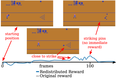
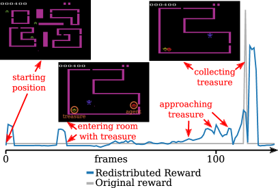
Figure A9: Observed return decomposition by RUDDER in two Atari games with long delayed rewards. Left: In the game Bowling, reward is only given after a turn which consist of multiple rolls. RUDDER identifies the actions that guide the ball in the right direction to hit all pins. Once the ball hit the pins, RUDDER detects the delayed reward associated with striking the pins down. In the figure only 100 frames are represented but the whole turn spans more than 200 frames. In the original game, the reward is given only at the end of the turn. Right: In the game Venture, reward is only obtained after picking the treasure. RUDDER guides the agent (red) towards the treasure (golden) via reward redistribution. Reward is redistributed to entering a room with treasure. Furthermore, the redistributed reward gradually increases as the agent approaches the treasure. For illustration purposes, the green curve shows the return redistribution before applying lambda. The environment only gives reward at the event of collecting treasure (blue).

Appendix A5 Discussion and Frequent Questions

RUDDER and reward rescaling.

RUDDER works with no rescaling, various rescalings, and sign function as we have confirmed in additional experiments. Rescaling ensures similar reward magnitudes across different Atari games, therefore the same hyperparameters can be used for all games. For LSTM and PPO, we only scale the original return by a constant factor, therefore do not change the problem and do not simplify it. The sign function, in contrast, may simplify the problem but may change the optimal policy.

RUDDER for infinite horizon: Continual Learning.

RUDDER assumes a finite horizon problem. For games and for most tasks in real world these assumptions apply: did you solve the task? (make tax declaration, convince a customer to buy, design a drug, drive a car to a location, assemble a car, build a building, clean the room, cook a meal, pass the Turing test). In general our approach can be extended to continual learning with discounted reward. Only the transformation of an immediate reward MDP to an MDP with episodic reward is no longer possible. However the delayed reward problem becomes more obvious and also more serious when not discounting the reward.

Is the LSTM in RUDDER a state-action value function?

For reward redistribution we assume an MDP with one reward (=return) at sequence end which can be predicted from the last state-action pair. When introducing the $\Delta$-states, the reward cannot be predicted from the last $\Delta$ and the task is no longer Markov. However the return can be predicted from the sequence of $\Delta$s. Since the $\Delta$s are mutually independent, the contribution of each $\Delta$ to the return must be stored in the hidden states of the LSTM to predict the final reward. The $\Delta$ can be generic as states and actions can be numbered and then the difference of this numbers can be used for $\Delta$.

In the applications like Atari with immediate rewards we give the accumulated reward at the end of the episode without enriching the states. This has a similar effect as using $\Delta$. We force the LSTM to build up an internal state which tracks the already accumulated reward.

True, the LSTM is the value function at time $t$ based on the $\Delta$ sub-sequence up to t. The LSTM prediction can be decomposed into two sub-predictions. The first sub-prediction is the contribution of the already known $\Delta$ sub-sequence up to t to the return (backward view). The second sub-prediction is the expected contribution of the unknown future sequence from t+1 onwards to the return (forward view). However, we are not interested in the second sub-prediction but only in the contribution of $\Delta_{t}$ to the prediction of the expected return. The second sub-prediction is irrelevant for our approach. We cancel the second sub-prediction via the differences of predictions. The difference at time t gives the contribution of $\Delta_{t}$ to the expected return.

Empirical confirmation: Four years ago, we started this research project with using LSTM as a value function, but we failed. This was the starting point for RUDDER. In the submission, we used LSTM predictions in artificial task (IV) as potential function for reward shaping, look-ahead advice, and look-back advice. Furthermore, we investigated LSTM as a value function for artificial task (II) but these results have not been included. At the time where RUDDER already solved the task, the LSTM error was too large to allow learning via a value function. Problem is the large variance of the returns at the beginning of the sequence which hinders LSTM learning (forward view). RUDDER LSTM learning was initiated by propagating back prediction errors at the sequence end, where the variance of the return is lower (backward view). These late predictions initiated the storing of key events at the sequence beginning even with high prediction errors. The redistributed reward at the key events led RUDDER solve the task. Concluding: at the time RUDDER solved the task, the early predictions are not learned due to the high variance of the returns. Therefore using the predictions as value function does not help (forward view).

Example: The agent has to take a key to open the door. Since it is an MDP, the agent is always aware to have the key indicated by a key bit to be on. The reward can be predicted in the last step. Using differences $\Delta$ the key bit is zero, except for the step where the agent takes the key. Thus, the LSTM has to store this event and will transfer reward to it.

Compensation reward.

The compensation corrects for prediction errors of $g$ ($g$ is the sum of $h$). The prediction error of $g$ can have two sources: (1) the probabilistic nature of the reward, (2) an approximation error of g for the expected reward. We aim to make (2) small and then the correction is only for the probabilistic nature of the reward. The compensation error depends on $g$, which, in turn, depends on the whole sequence. The dependency on state-action pairs from $t=0$ to $T-1$ is viewed as random effect, therefore the compensation reward only depends on the last state-action pair.

That $h_{t}$ and $R_{t+1}$ depends only on $(s_{t},a_{t},s_{t-1},a_{t-1})$ is important to prove Theorem 3. Then $a_{t-1}$ cancels and the advantage function remains the same.

Connection theory and algorithms.

Theorem 1 and Theorem 2 ensure that the algorithms are correct since the optimal policies do not change even for non-optimal return decompositions. In contrast to TD methods which are biased, Theorem 3 shows that the update rule $Q$-value estimation is unbiased when assuming optimal decomposition. Theorem 4 explicitly derives optimality conditions for the expected sum of delayed rewards “kappa” and measures the distance to optimality. This “kappa” is used for learning and is explicitly estimated to correct learning if an optimal decomposition cannot be assured. The theorems are used to justify following learning methods (A) and (B):

(A) Q-value estimation: (i) Direct Q-value estimation (not Q-learning) according to Theorem 3 is given in Eq. (9) when an optimal decomposition is assumed. (ii) Q-value estimation with correction by kappa according to Theorem 4, when optimal decomposition is not assumed. Here kappa is learned by TD as given in Eq. (10). (iii) Q-value estimation using eligibility traces. (B) Policy gradient: Theorems are used as for Q-value estimation as in (A) but now the Q-values serve for policy gradient. (C) Q-learning: Here the properties in Theorem 3 and Theorem 4 are ignored.

We also shows variants (not in the main paper) on page 31 and 32 of using kappa “Correction of the reward redistribution” by reward shaping with kappa and “Using kappa as auxiliary task in predicting the return for return decomposition”.

Optimal Return Decomposition, contributions and policy.

The Q-value $q^{\pi}$ depends on a particular policy $\pi$. The function h depends on policy $\pi$ since h predicts the expected return ($E_{\pi}[\tilde{R}_{T+1}]$) which depends on $\pi$. Thus, both return decomposition and optimal return decomposition are defined for a particular policy $\pi$. A reward redistribution from a return decomposition leads to a return equivalent MDP. Return equivalent MDPs are defined via all policies even if the reward redistribution was derived from a particular policy. A reward redistribution depends only on the state-action sequence but not on the policy that generated this sequence. Also $\Delta$ does not depend on a policy.

Optimal policies are preserve for every state.

We assume all states are reachable via at least one non-zero transition probability to each state and policies that have a non-zero probability for each action due to exploration. For an MDP being optimal in the initial state is the same as being optimal in every reachable state. This follows from recursively applying the Bellman optimality equation to the initial value function. The values of the following states must be optimal otherwise the initial value function is smaller. Only states to which the transition probability is zero the Bellman optimality equation does not determine the optimality.

All RL algorithms are suitable. For example we applied TD, Monte Carlo, Policy Gradient, which all work faster with the new MDP.

Limitations.

In all of the experiments reported in this manuscript, we show that RUDDER significantly outperforms other methods for delayed reward problems. However, RUDDER might not be effective when the reward is not delayed since LSTM learning takes extra time and has problems with very long sequences. Furthermore, reward redistribution may introduce disturbing spurious reward signals.

Appendix A6 Additional Related Work

Delayed Reward.

To learn delayed rewards there are three phases to consider: (i) discovering the delayed reward, (ii) keeping information about the delayed reward, (iii) learning to receive the delayed reward to secure it for the future. Recent successful reinforcement learning methods provide solutions to one or more of these phases. Most prominent are Deep $Q$-Networks (DQNs) [81, 82], which combine $Q$-learning with convolutional neural networks for visual reinforcement learning [69]. The success of DQNs is attributed to experience replay [74], which stores observed state-reward transitions and then samples from them. Prioritized experience replay [109, 58] advanced the sampling from the replay memory. Different policies perform exploration in parallel for the Ape-X DQN and share a prioritized experience replay memory [58]. DQN was extended to double DQN (DDQN) [134, 135] which helps exploration as the overestimation bias is reduced. Noisy DQNs [26] explore by a stochastic layer in the policy network (see [48, 110]). Distributional $Q$-learning [10] profits from noise since means that have high variance are more likely selected. The dueling network architecture [138, 139] separately estimates state values and action advantages, which helps exploration in unknown states. Policy gradient approaches [145] explore via parallel policies, too. A2C has been improved by IMPALA through parallel actors and correction for policy-lags between actors and learners [24]. A3C with asynchronous gradient descent [80] and Ape-X DPG [58] also rely on parallel policies. Proximal policy optimization (PPO) extends A3C by a surrogate objective and a trust region optimization that is realized by clipping or a Kullback-Leibler penalty [115].

Recent approaches aim to solve learning problems caused by delayed rewards. Function approximations of value functions or critics [82, 80] bridge time intervals if states associated with rewards are similar to states that were encountered many steps earlier. For example, assume a function that has learned to predict a large reward at the end of an episode if a state has a particular feature. The function can generalize this correlation to the beginning of an episode and predict already high reward for states possessing the same feature. Multi-step temporal difference (TD) learning [127, 128] improved both DQNs and policy gradients [47, 80]. AlphaGo and AlphaZero learned to play Go and Chess better than human professionals using Monte Carlo Tree Search (MCTS) [116, 117]. MCTS simulates games from a time point until the end of the game or an evaluation point and therefore captures long delayed rewards. Recently, world models using an evolution strategy were successful [42]. These forward view approaches are not feasible in probabilistic environments with a high branching factor of state transition.

Backward View.

We propose learning from a backward view, which either learns a separate model or analyzes a forward model. Examples of learning a separate model are to trace back from known goal states [23] or from high reward states [36]. However, learning a backward model is very challenging. When analyzing a forward model that predicts the return then either sensitivity analysis or contribution analysis may be utilized. The best known backward view approach is sensitivity analysis (computing the gradient) like ”Backpropagation through a Model´´ [86, 101, 102, 142, 5]. Sensitivity analysis has several drawbacks: local minima, instabilities, exploding or vanishing gradients, and proper exploration [48, 110]. The major drawback is that the relevance of actions is missed since sensitivity analysis does not consider their contribution to the output but only their effect on the output when slightly perturbing them.

We use contribution analysis since sensitivity analysis has serious drawbacks. Contribution analysis determines how much a state-action pair contributes to the final prediction. To focus on state-actions which are most relevant for learning is known from prioritized sweeping for model-based reinforcement learning [85]. Contribution analysis can be done by computing differences of return predictions when adding another input, by zeroing out an input and then compute the change in the prediction, by contribution-propagation [71], by a contribution approach [94], by excitation backprop [147], by layer-wise relevance propagation (LRP) [3], by Taylor decomposition [3, 83], or by integrated gradients (IG) [125].

LSTM.

LSTM was already used in reinforcement learning [112] for advantage learning [4], for constructing a potential function for reward shaping by representing the return by a sum of LSTM outputs across an episode [124], and learning policies [44, 80, 45].

Reward Shaping, Look-Ahead Advice, Look-Back Advice.

Redistributing the reward is fundamentally different from reward shaping [87, 143], look-ahead advice and look-back advice [144]. However, these methods can be viewed as a special case of reward redistribution that result in an MDP that is return-equivalent to the original MDP as is shown in Section A2.2. On the other hand every reward function can be expressed as look-ahead advice [43]. In contrast to these methods, reward redistribution is not limited to potential functions, where the additional reward is the potential difference, therefore it is a more general concept than shaping reward or look-ahead/look-back advice. The major difference of reward redistribution to reward shaping, look-ahead advice, and look-back advice is that the last three keep the original rewards. Both look-ahead advice and look-back advice have not been designed for replacing for the original rewards. Since the original reward is kept, the reward redistribution is not optimal according to Section A2.6.1. The original rewards may have long delays that cause an exponential slow-down of learning. The added reward improves sampling but a delayed original reward must still be transferred to the $Q$-values of early states that caused the reward. The concept of return-equivalence of SDPs resulting from reward redistributions allows to eliminate the original reward completely. Reward shaping can replace the original reward. However, it only depends on states but not on actions, and therefore, it cannot identify relevant actions without the original reward.

Appendix A7 Markov Decision Processes with Undiscounted Rewards

We focus on Markov Decision Processes (MDPs) with undiscounted rewards, since the relevance but also the problems of a delayed reward can be considerably decreased by discounting it. Using discounted rewards both the bias correction in TD as well as the variance of MC are greatly reduced. The correction amount decreases exponentially with the delay steps, and also the variance contribution to one state decreases exponentially with the delay of the reward.

MDPs with undiscounted rewards are either finite horizon or process absorbing states without reward. The former can always be described by the latter.

A7.1 Properties of the Bellman Operator in MDPs with Undiscounted Rewards

At each time $t$ the environment is in some state $s=s_{t}\in\mathcal{S}$. The agent takes an action $a=a_{t}\in\mathcal{A}$ according to policy $\pi$, which causes a transition of the environment to state $s^{\prime}=s_{t+1}\in\mathcal{S}$ and a reward $r=r_{t+1}\in\mathcal{R}$ for the agent with probability $p(s^{\prime},r\mid s,a)$.

The Bellman operator maps a action-value function $q=q(s,a)$ to another action-value function. We do not require that $q$ are $Q$-values and that $r$ is the actual reward. We define the Bellman operator $\mathrm{T}^{\pi}$ for policy $\pi$ as:

$$\mathrm{T}^{\pi}\left[q\right](s,a)\ =\ \sum_{s^{\prime},r}p(s^{\prime},r\mid s,a)\ \left[r\ +\ \sum_{a^{\prime}}\pi(a^{\prime}\mid s^{\prime})\ q(s^{\prime},a^{\prime})\right]\ .$$ (A276)

We often rewrite the operator as

$$\mathrm{T}^{\pi}\left[q\right](s,a)\ =\ r(s,a)\ +\ \mathbf{\mathrm{E}}_{s^{\prime},a^{\prime}}\left[q(s^{\prime},a^{\prime})\right]\ ,$$ (A277)

where

$$r(s,a)\ =\ \sum_{r}r\ p(r\mid s,a)\ ,$$ (A278)

$$\mathbf{\mathrm{E}}_{s^{\prime},a^{\prime}}\left[q(s^{\prime},a^{\prime})\right]\ =\ \sum_{s^{\prime}}p(s^{\prime}\mid s,a)\ \sum_{a^{\prime}}\pi(a^{\prime}\mid s^{\prime})\ q(s^{\prime},a^{\prime})\ .$$ (A279)

We did not explicitly express the dependency on the policy $\pi$ and the state-action pair $(s,a)$ in the expectation $\mathbf{\mathrm{E}}_{s^{\prime},a^{\prime}}$. A more precise way would be to write $\mathbf{\mathrm{E}}^{\pi}_{s^{\prime},a^{\prime}}\left[.\mid s,a\right]$.

More generally, we have

$$\mathrm{T}^{\pi}\left[q\right](s,a)\ =\ g(s,a)\ +\ \mathbf{\mathrm{E}}_{s^{\prime},a^{\prime}}\left[q(s^{\prime},a^{\prime})\right]\ .$$ (A280)

In the following we show properties for this general formulation.

A7.1.1 Monotonically Increasing and Continuous

We assume the general formulation Eq. (A280) of the Bellman operator. Proposition 2.1 on pages 22-23 in Bertsekas and Tsitsiklis, 1996, [14] shows that a fixed point $q^{\pi}$ of the Bellman operator exists and that for every $q$:

$$q^{\pi}\ =\ \mathrm{T}^{\pi}\left[q^{\pi}\right]$$ (A281)

$$q^{\pi}\ =\ \lim_{k\to\infty}\left(\mathrm{T}^{\pi}\right)^{k}q\ .$$ (A282)

The fixed point equation

$$q^{\pi}\ =\ \mathrm{T}^{\pi}\left[q^{\pi}\right]$$ (A283)

is called Bellman equation or Poisson equation. For the Poisson equation see Equation 33 to Equation 37 for the undiscounted case and Equation 34 and Equation 43 for the discounted case in Alexander Veretennikov, 2016, [137]. This form of the Poisson equation describes the Dirichlet boundary value problem. The Poisson equation is

$$q^{\pi}(s,a)\ +\ \bar{g}\ =\ g(s,a)\ +\ \mathbf{\mathrm{E}}_{s^{\prime},a^{\prime}}\left[q(s^{\prime},a^{\prime})\mid s,a\right]\ ,$$ (A284)

where $\bar{g}$ is the long term average reward or the expected value of the reward for the stationary distribution:

$$\bar{g}\ =\ \lim_{T\to\infty}\frac{1}{T+1}\sum_{t=0}^{T}g(s_{t},a_{t})\ .$$ (A285)

We assume $\bar{g}=0$ since after some time the agent does no longer receive reward in MDPs with finite time horizon or in MDPs with absorbing states that have zero reward.

$\mathrm{T}^{\pi}$ is monotonically increasing in its arguments [14]. For $q_{1}$ and $q_{2}$ with the component-wise condition $q_{1}\geqslant q_{2}$, we have

$$\mathrm{T}^{\pi}\left[q_{1}\right](s,a)\ -\ \mathrm{T}^{\pi}\left[q_{2}\right](s,a)$$ (A286)

$$=\ \left(g(s,a)\ +\ \mathbf{\mathrm{E}}_{s^{\prime},a^{\prime}}\left[q_{1}(s^{\prime},a^{\prime})\right]\right)\ -\ \left(g(s,a)\ +\ \mathbf{\mathrm{E}}_{s^{\prime},a^{\prime}}\left[q_{2}(s^{\prime},a^{\prime})\right]\right)$$

$$=\ \mathbf{\mathrm{E}}_{s^{\prime},a^{\prime}}\left[q_{1}(s^{\prime},a^{\prime})\ -\ q_{2}(s^{\prime},a^{\prime})\right]\ \geqslant\ 0\ ,$$

where “$\geqslant$” is component-wise. The last inequality follows from the component-wise condition $q_{1}\geqslant q_{2}$.

We define the norm $\|.\|_{\infty}$, which gives the maximal difference of the $Q$-values:

$$\|q_{1}\ -\ q_{2}\|_{\infty}\ =\ \underset{s,a}{\max}\left|q_{1}(s,a)\ -\ q_{2}(s,a)\right|\ .$$ (A287)

$\mathrm{T}$ is a non-expansion mapping for $q_{1}$ and $q_{2}$:

$$\|\mathrm{T}^{\pi}\left[q_{1}\right]\ -\ \mathrm{T}^{\pi}\left[q_{2}\right]\|_{\infty}\ =\ \underset{s,a}{\max}\left|\mathrm{T}[q_{1}](s,a)\ -\ \mathrm{T}[q_{2}](s,a)\right|$$ (A288)

$$=\ \underset{s,a}{\max}\left|\left[g(s,a)\ +\ \sum_{s^{\prime}}p(s^{\prime}\mid s,a)\ \sum_{a^{\prime}}\pi(a^{\prime}\mid s^{\prime})\ q_{1}(s^{\prime},a^{\prime})\right]\ -\ \right.$$

$$\ \ \ \left.\left[g(s,a)\ +\ \sum_{s^{\prime}}p(s^{\prime}\mid s,a)\sum_{a^{\prime}}\pi(a^{\prime}\mid s^{\prime})\ q_{2}(s^{\prime},a^{\prime})\right]\right|$$

$$=\ \underset{s,a}{\max}\left|\sum_{s^{\prime}}p(s^{\prime}\mid s,a)\ \sum_{a^{\prime}}\pi(a^{\prime}\mid s^{\prime})\ \left(q_{1}(s^{\prime},a^{\prime})\ -\ q_{2}(s^{\prime},a^{\prime})\right)\right|$$

$$\leqslant\ \underset{s,a}{\max}\sum_{s^{\prime}}p(s^{\prime}\mid s,a)\ \sum_{a^{\prime}}\pi(a^{\prime}\mid s^{\prime})\ \left|q_{1}(s^{\prime},a^{\prime})\ -\ q_{2}(s^{\prime},a^{\prime})\right|$$

$$\leqslant\ \underset{s^{\prime},a^{\prime}}{\max}\left|q_{1}(s^{\prime},a^{\prime})\ -\ q_{2}(s^{\prime},a^{\prime})\right|\ =\ \|q_{1}\ -\ q_{2}\|_{\infty}\ .$$

The first inequality is valid since the absolute value is moved into the sum. The second inequality is valid since the expectation depending on $(s,a)$ is replaced by a maximum that does not depend on $(s,a)$. Consequently, the operator $\mathrm{T}^{\pi}$ is continuous.

A7.1.2 Contraction for Undiscounted Finite Horizon

For time-aware states, we can define another norm with $0<\eta<1$ which allows for a contraction mapping:

$$\|q_{1}\ -\ q_{2}\|_{\infty,t}\ =\ \max_{t=0}^{T}\eta^{T-t+1}\ \underset{s_{t},a}{\max}\left|q_{1}(s_{t},a)\ -\ q_{2}(s_{t},a)\right|\ .$$ (A289)

$\mathrm{T}^{\pi}$ is a contraction mapping for $q_{1}$ and $q_{2}$ [14]:

$$\|\mathrm{T}^{\pi}\left[q_{1}\right]\ -\ \mathrm{T}^{\pi}\left[q_{2}\right]\|_{\infty,t}\ =\ \max_{t=0}^{T}\ \eta^{T-t+1}\ \underset{s_{t},a}{\max}\left|\mathrm{T}[q_{1}](s_{t},a)\ -\ \mathrm{T}[q_{2}](s_{t},a)\right|$$ (A290)

$$=\ \max_{t=0}^{T}\ \eta^{T-t+1}\ \underset{s_{t},a}{\max}\left|\left[g(s_{t},a)\ +\ \sum_{s_{t+1}}p(s_{t+1}\mid s_{t},a)\ \sum_{a^{\prime}}\pi(a^{\prime}\mid s^{\prime})\ q_{1}(s_{t+1},a^{\prime})\right]\ -\ \right.$$

$$\ \ \ \left.\left[g(s_{t},a)\ +\ \sum_{s_{t+1}}p(s_{t+1}\mid s_{t},a)\sum_{a^{\prime}}\pi(a^{\prime}\mid s^{\prime})\ q_{2}(s_{t+1},a^{\prime})\right]\right|$$

$$=\ \max_{t=0}^{T}\ \eta^{T-t+1}\ \underset{s_{t},a}{\max}\left|\sum_{s_{t+1}}p(s_{t+1}\mid s_{t},a)\ \sum_{a^{\prime}}\pi(a^{\prime}\mid s^{\prime})\ \left[q_{1}(s_{t+1},a^{\prime})\ -\ q_{2}(s_{t+1},a^{\prime})\right]\right|$$

$$\leqslant\ \max_{t=0}^{T}\ \eta^{T-t+1}\ \underset{s_{t},a}{\max}\sum_{s_{t+1}}p(s_{t+1}\mid s_{t},a)\ \sum_{a^{\prime}}\pi(a^{\prime}\mid s^{\prime})\ \left|q_{1}(s_{t+1},a^{\prime})\ -\ q_{2}(s_{t+1},a^{\prime})\right|$$

$$\leqslant\ \max_{t=0}^{T}\ \eta^{T-t+1}\ \underset{s_{t+1},a^{\prime}}{\max}\ \left|q_{1}(s_{t+1},a^{\prime})\ -\ q_{2}(s_{t+1},a^{\prime})\right|$$

$$\leqslant\ \max_{t=0}^{T}\ \eta\ \eta^{T-(t+1)+1}\ \underset{s_{t+1},a^{\prime}}{\max}\left|q_{1}(s_{t+1},a^{\prime})\ -\ q_{2}(s_{t+1},a^{\prime})\right|$$

$$=\ \eta\ \max_{t=1}^{T+1}\ \eta^{T-t+1}\underset{s_{t},a^{\prime}}{\max}\left|q_{1}(s_{t},a^{\prime})\ -\ q_{2}(s_{t},a^{\prime})\right|$$

$$=\ \eta\ \max_{t=0}^{T}\ \eta^{T-t+1}\ \underset{s_{t},a^{\prime}}{\max}\left|q_{1}(s_{t},a^{\prime})\ -\ q_{2}(s_{t},a^{\prime})\right|$$

$$=\ \eta\ \|q_{1}\ -\ q_{2}\|_{\infty,t}\ .$$

The equality in the last but one line stems from the fact that all $Q$-values at $t=T+1$ are zero and that all $Q$-values at $t=1$ have the same constant value.

Furthermore, all $q$ values are equal to zero for additionally introduced states at $t=T+1$ since for $t>T+1$ all rewards are zero. We have

$$q^{\pi}\ =\ \mathrm{T}^{T}\left[q\right]\ ,$$ (A291)

which is correct for additionally introduced states at time $t=T+1$ since they are zero. Then, in the next iteration $Q$-values of states at time $t=T$ are correct. After iteration $i$, $Q$-values of states at time $t=T-i+1$ are correct. This iteration is called the “backward induction algorithm” [95, 96]. If we perform this iteration for a policy $\pi$ instead of the optimal policy, then this procedure is called “policy evaluation algorithm” [95, 96].

A7.1.3 Contraction for Undiscounted Infinite Horizon With Absorbing States

A stationary policy is proper if there exists an integer $n$ such that from any initial state $x$ the probability of achieving the terminal state after $n$ steps is strictly positive.

If all terminal states are absorbing and cost/reward free and if all stationary policies are proper the Bellman operator is a contraction mapping with respect to a weighted sup-norm.

The fact that the Bellman operator is a contraction mapping with respect to a weighted sup-norm has been proved in Tseng, 1990, in Lemma 3 with equation (13) and text thereafter [132]. Also Proposition 1 in Bertsekas and Tsitsiklis, 1991, [13], Theorems 3 and 4(b) & 4(c) in Tsitsiklis, 1994, [133], and Proposition 2.2 on pages 23-24 in Bertsekas and Tsitsiklis, 1996, [14] have proved the same fact.

A7.1.4 Fixed Point of Contraction is Continuous wrt Parameters

The mean $q^{\pi}$ and variance $V^{\pi}$ are continuous with respect to $\pi$, that is $\pi(a^{\prime}\mid s^{\prime})$, with respect to the reward distribution $p(r\mid s,a)$ and with respect to the transition probabilities $p(s^{\prime}\mid s,a)$.

A complete metric space or a Cauchy space is a space where every Cauchy sequence of points has a limit in the space, that is, every Cauchy sequence converges in the space. The Euclidean space $\mathbb{R}^{n}$ with the usual distance metric is complete. Lemma 2.5 in Jachymski, 1996, is [62]:

Theorem A11 (Jachymski: complete metric space).

Let $(X,d)$ be a complete metric space, and let $(P,d_{P})$ be a metric space. Let $F:P\times X\to X$ be continuous in the first variable and contractive in the second variable with the same Lipschitz constant $\alpha<1$. For $\bm{p}\in P$, let $\bm{x}^{*}(\bm{p})$ be the unique fixed point of the map $\bm{x}\to F(\bm{p},\bm{x})$. Then the mapping $\bm{x}^{*}$ is continuous.

This theorem is Theorem 2.3 in Frigon, 2007, [27]. Corollary 4.2 in Feinstein, 2016, generalized the theorem to set valued operators, that is, these operators may have more than one fixed point [25] (see also [67]). All mappings $F(p,.)$ must have the same Lipschitz constant $\alpha<1$.

A locally compact space is a space where every point has a compact neighborhood. $\mathbb{R}^{n}$ is locally compact as a consequence of the Heine-Borel theorem. Proposition 3.2 in Jachymski, 1996, is [62]:

Theorem A12 (Jachymski: locally compact complete metric space).

Let $(X,d)$ be a locally compact complete metric space, and let $(P,d_{P})$ be a metric space. Let $F:P\times X\to X$ be continuous in the first variable and contractive in the second variable with not necessarily the same Lipschitz constant. For $\bm{p}\in P$, let $\bm{x}^{*}(\bm{p})$ be the unique fixed point of the map $\bm{x}\to F(\bm{p},\bm{x})$. Then the mapping $\bm{x}^{*}$ is continuous.

This theorem is Theorem 2.5 in Frigon, 2007, [27] and Theorem 2 in Kwiecinski, 1992, [70]. The mappings $F(p,.)$ can have different Lipschitz constants.

A7.1.5 t-fold Composition of the Operator

We define the Bellman operator as

$$\mathrm{T}^{\pi}\left[q\right](s,a)\ =\ g(s,a)\ +\ \sum_{s^{\prime}}p(s^{\prime}\mid s,a)\ \sum_{a^{\prime}}\pi(a^{\prime}\mid s^{\prime})\ q(s^{\prime},a^{\prime})$$ (A292)

$$=\ g(s,a)\ +\ \bm{q}^{T}\bm{p}(s,a)\ ,$$

where $\bm{q}$ is the vector with value $q(s^{\prime},a^{\prime})$ at position $(s^{\prime},a^{\prime})$ and $\bm{p}(s,a)$ is the vector with value $p(s^{\prime}\mid s,a)\pi(a^{\prime}\mid s^{\prime})$ at position $(s^{\prime},a^{\prime})$.

In vector notation we obtain the Bellman equation or Poisson equation. For the Poisson equation see Equation 33 to Equation 37 for the undiscounted case and Equation 34 and Equation 43 for the discounted case in Alexander Veretennikov, 2016, [137]. This form of the Poisson equation describes the Dirichlet boundary value problem. The Bellman equation or Poisson equation is

$$\mathrm{T}^{\pi}\left[\bm{q}\right]\ =\ \bm{g}\ +\ \bm{P}\ \bm{q}\ ,$$ (A293)

where $\bm{P}$ is the row-stochastic matrix with $p(s^{\prime}\mid s,a)\pi(a^{\prime}\mid s^{\prime})$ at position $((s,a),(s^{\prime},a^{\prime}))$.

The Poisson equation is

$$\bm{q}^{\pi}\ +\ \bar{g}\bm{1}\ =\ \bm{g}\ +\ \bm{P}\ \bm{q}\ ,$$ (A294)

where $\bm{1}$ is the vector of ones and $\bar{\bm{g}}$ is the long term average reward or the expected value of the reward for the stationary distribution:

$$\bar{g}\ =\ \lim_{T\to\infty}\frac{1}{T+1}\sum_{t=0}^{T}g(s_{t},a_{t})\ .$$ (A295)

We assume $\bar{g}=0$ since after some time the agent does no longer receive reward for MDPs with finite time horizon or MDPs with absorbing states that have zero reward.

Since $\bm{P}$ is a row-stochastic matrix, the Perron-Frobenius theorem says that (1) $\bm{P}$ has as largest eigenvalue 1 for which the eigenvector corresponds to the steady state and (2) the absolute value of each (complex) eigenvalue is smaller or equal 1. Only the eigenvector to the eigenvalue 1 has purely positive real components.

Equation 7 of Bertsekas and Tsitsiklis, 1991, [13] states

$$\left(\mathrm{T}^{\pi}\right)^{t}\left[\bm{q}\right]\ =\ \sum_{k=0}^{t-1}\bm{P}^{k}\ \bm{g}\ +\ \bm{P}^{t}\ \bm{q}\ .$$ (A296)

If $\bm{p}$ is the stationary distribution vector for $\bm{P}$, that is,

$$\lim_{k\to\infty}\bm{P}^{k}\ =\ \bm{1}\ \bm{p}^{T}$$ (A297)

$$\lim_{k\to\infty}\bm{p}_{0}^{T}\bm{P}^{k}\ =\ \bm{p}^{T}$$ (A298)

then

$$\lim_{k\to\infty}\frac{1}{k}\sum_{i=0}^{k-1}\bm{P}^{i}\ =\ \bm{1}\ \bm{p}^{T}$$ (A299)

$$\lim_{k\to\infty}\frac{1}{k}\sum_{i=0}^{k-1}\bm{p}_{0}^{T}\bm{P}^{i}\ =\ \bm{p}^{T}\ .$$ (A300)

A7.2 Q-value Transformations: Shaping Reward, Baseline, and Normalization

The Bellman equation for the action-value function $q^{\pi}$ is

$$q^{\pi}(s,a)\ =\ \sum_{s^{\prime},r}p(s^{\prime},r\mid s,a)\ \left[r\ +\ \sum_{a^{\prime}}\pi(a^{\prime}\mid s^{\prime})\ q^{\pi}(s^{\prime},a^{\prime})\right]\ .$$ (A301)

The expected return at time $t=0$ is:

$$v_{0}\ =\ \sum_{s_{0}}p(s_{0})\ v(s_{0})\ .$$ (A302)

As introduced for the REINFORCE algorithm, we can subtract a baseline $v_{0}$ from the return. We subtract the baseline $v_{0}$ from the last reward. Therefore, for the new reward $\bar{R}$ we have $\bar{R}_{t}=R_{t}$ for $t\leqslant T$ and $\bar{R}_{T+1}=R_{T+1}-v_{0}$. Consequently, $\bar{q}(s_{t},a_{t})=q(s_{t},a_{t})-v_{0}$ for $t\leqslant T$.

The TD update rules are:

$$q(s_{t},a_{t})\ \longleftarrow\ q(s_{t},a_{t})\ +\ \alpha\left(r_{t}\ +\ \sum_{a}\pi(a\mid s_{t+1})\ q(s_{t+1},a)\ -\ q(s_{t},a_{t})\right)\ .$$ (A303)

The $\delta$-errors are

$$R_{t+1}\ +\ \sum_{a}\pi(a\mid s_{t+1})\ q(s_{t+1},a)\ -\ q(s_{t},a_{t})$$

$$=\ R_{t+1}\ +\ \sum_{a}\pi(a\mid s_{t+1})\ (q(s_{t+1},a)-v_{0})\ -\ (q(s_{t},a_{t})-v_{0})$$

$$=\ \bar{R}_{t+1}\ +\ \sum_{a}\pi(a\mid s_{t+1})\ \bar{q}(s_{t+1},a)\ -\ \bar{q}(s_{t},a_{t})$$ (A304)

and for the last step

$$R_{T+1}\ -\ q(s_{T},a_{T})\ =\ (R_{T+1}\ -\ v_{0})\ -\ (q(s_{T},a_{T})\ -\ v_{0})$$ (A305)

$$=\ \bar{R}_{T+1}\ -\ \bar{q}(s_{T},a_{T})\ .$$

If we set

$$\bar{q}(s_{t},a_{t})\ =\ \begin{cases}q(s_{t},a_{t})\ -\ v_{0}\ ,&\text{for }t\leqslant T\ .\end{cases}$$ (A306)

$$\bar{R}_{t}\ =\ \begin{cases}R_{t}\ ,&\text{for }t\leqslant T\\ R_{T+1}\ -\ v_{0}\ ,&\text{for }t=T+1\ ,\end{cases}$$ (A307)

then the $\delta$-errors and the updates remain the same for $q$ and $\bar{q}$. We are equally far away from the optimal solution in both cases.

Removing the offset $v_{0}$ at the end by $\bar{R}_{T+1}=R_{T+1}-v_{0}$, can also be derived via reward shaping. However, the offset has to be added at the beginning: $\bar{R}_{1}=R_{1}+v_{0}$. Reward shaping requires for the shaping reward $F$ and a potential function $\Phi$ [87, 143]:

$$F(s_{t},a_{t},s_{t+1})\ =\ \Phi(s_{t+1})-\Phi(s_{t})\ .$$ (A308)

For introducing a reward of $c$ at time $t=k$ and removing it from time $t=m<k$ we set:

$$\Phi(s_{t})\ =\ \begin{cases}0\ ,&\text{for }t\leqslant m\ ,\\ -c\ ,&\text{for }m+1\leqslant t\leqslant k\ ,\\ 0\ ,&\text{for }t>k\ ,\end{cases}$$ (A309)

then the shaping reward is

$$F\big{(}s_{t},a_{t},s_{t+1}\big{)}\ =\ \begin{cases}0\ ,&\text{for }t<m\ ,\\ -c\ ,&\text{for }t=m\ ,\\ 0\ ,&\text{for }m+1\leqslant t<k\ ,\\ c\ ,&\text{for }t=k\ ,\\ 0\ ,&\text{for }t>k\ .\end{cases}$$ (A310)

For $k=T$, $m=0$, and $c=-v_{0}$ we obtain above situation but with $\bar{R}_{1}=R_{1}+v_{0}$ and $\bar{R}_{T+1}=R_{T+1}-v_{0}$, that is, $v_{0}$ is removed at the end and added at the beginning. All $Q$-values except $q(s_{0},a_{0})$ are decreased by $v_{0}$. In the general case, all $Q$-values $q(s_{t},a_{t})$ with $m+1\leqslant t\leqslant k$ are increased by $c$.

$Q$-value normalization: We apply reward shaping [87, 143] for normalization of the $Q$-values. The potential $\Phi(s)$ defines the shaping reward $F(s_{t},a_{t},s_{t+1})=\Phi(s_{t+1})-\Phi(s_{t})$. The optimal policies do not change and the $Q$-values become

$$q^{\mathrm{new}}(s_{t},a_{t})\ =\ q(s_{t},a_{t})\ -\ \Phi(s_{t})\ .$$ (A311)

We change the $Q$-values for all $1\leqslant t\leqslant T$, but not for $t=0$ and $t=T+1$. The first and the last $Q$-values are not normalized. All the shaped reward is added/subtracted to/from the initial and the last reward.

• The maximal $Q$-values are zero and the non-optimal $Q$-values are negative for all $1\leqslant t\leqslant T$:

  $$\Phi(s_{t})\ =\ \max_{a}q(s_{t},a)\ .$$ (A312)

• The minimal $Q$-values are zero and all others $Q$-values are positive for all $1\leqslant t\leqslant T-1$:

  $$\Phi(s_{t})\ =\ \min_{a}q(s_{t},a)\ .$$ (A313)

A7.3 Alternative Definition of State Enrichment

Next, we define state-enriched processes $\tilde{\mathcal{P}}$ compared to $\mathcal{P}$. The state $\tilde{s}$ of $\tilde{\mathcal{P}}$ is enriched with a deterministic information compared to a state $s$ of $\mathcal{P}$. The enriched information in $\tilde{s}$ can be computed from the state-action pair $(\tilde{s},a)$ and the reward $r$. Enrichments may be the accumulated reward, count of the time step, a count how often a certain action has been performed, a count how often a certain state has been visited, etc. Givan et al. have already shown that state-enriched Markov decision processes (MDPs) preserve the optimal action-value and action sequence properties as well as the optimal policies of the model [34]. Theorem 7 and Corollary 9.1 in Givan et al. proved these properties [34] by bisimulations (stochastically bisimilar MDPs). A homomorphism between MDPs maps a MDP to another one with corresponding reward and transitions probabilities. Ravindran and Barto have shown that solving the original MDP can be done by solving a homomorphic image [99]. Therefore, Ravindran and Barto have also shown that state-enriched MDPs preserve the optimal action-value and action sequence properties. Li et al. give an overview over state abstraction or state aggregation for MDPs, which covers state-enriched MDPs [73].

Definition A14.

A decision process $\tilde{\mathcal{P}}$ is state-enriched compared to a decision process $\mathcal{P}$ if following conditions hold. If $\tilde{s}$ is the state of $\tilde{\mathcal{P}}$, then there exists a function $f:\tilde{s}\to s$ with $f(\tilde{s})=s$, where $s$ is the state of $\mathcal{P}$. There exists a function $g:\tilde{s}\to\mathcal{R}$, where $g(\tilde{s})$ gives the additional information of state $\tilde{s}$ compared to $f(\tilde{s})$. There exists a function $\nu$ with $\nu(f(\tilde{s}),g(\tilde{s}))=\tilde{s}$, that is, the state $\tilde{s}$ can be constructed from the original state and the additional information. There exists a function $H$ with $h(\tilde{s}^{\prime})=H(r,\tilde{s},a)$, where $\tilde{s}^{\prime}$ is the next state and $r$ the reward. $H$ ensures that $h(\tilde{s}^{\prime})$ of the next state $\tilde{s}^{\prime}$ can be computed from reward $r$, actual state $\tilde{s}$, and the actual action $a$. Consequently, $\tilde{s}^{\prime}$ can be computed from $(r,\tilde{s},a)$. For all $\tilde{s}$ and $\tilde{s}^{\prime}$ following holds:

$$\tilde{p}(\tilde{s}^{\prime},r\mid\tilde{s},a)\ =\ p(f(\tilde{s}^{\prime}),r\mid f(\tilde{s}),a)\ ,$$ (A314)

$$\tilde{p}_{0}(\tilde{s}_{0})\ =\ p_{0}(f(\tilde{s}_{0}))\ ,$$ (A315)

where $\tilde{p}_{0}$ and $p_{0}$ are the probabilities of the initial states of $\tilde{\mathcal{P}}$ and $\mathcal{P}$, respectively.

If the reward is deterministic, then $\tilde{p}(\tilde{s}^{\prime},r\mid\tilde{s},a)=\tilde{p}(\tilde{s}^{\prime}\mid\tilde{s},a)$ and $\tilde{p}_{0}(\tilde{s}_{0},r)=\tilde{p}_{0}(\tilde{s}_{0})$.

We proof the following theorem, even if it has been proved several times as mention above.

Theorem A13.

If decision process $\tilde{\mathcal{P}}$ is state-enriched compared to $\mathcal{P}$, then for each optimal policy $\tilde{\pi}^{*}$ of $\tilde{\mathcal{P}}$ there exists an equivalent optimal policy $\pi^{*}$ of $\mathcal{P}$, and vice versa, with $\tilde{\pi}^{*}(\tilde{s})=\pi^{*}(f(\tilde{s}))$. The optimal return is the same for $\tilde{\mathcal{P}}$ and $\mathcal{P}$.

Proof.

We proof by induction that $\tilde{q}^{\tilde{\pi}}(\tilde{s},a)=q^{\pi}(f(\tilde{s}),a)$ if $\tilde{\pi}(\tilde{s})=\pi(f(\tilde{s}))$.

Basis: The end of the sequence. For $t\geqslant T$ we have $\tilde{q}^{\tilde{\pi}}(\tilde{s},a)=q^{\pi}(f(\tilde{s}),a)=0$, since no policy receives reward for $t\geqslant T$.

Inductive step ($t\to t-1$): Assume $\tilde{q}^{\tilde{\pi}}(\tilde{s}^{\prime},a^{\prime})=q^{\pi}(f(\tilde{s}^{\prime}),a^{\prime})$ for the next state $\tilde{s}^{\prime}$ and next action $a^{\prime}$.

$$\tilde{q}^{\tilde{\pi}}(\tilde{s},a)\ =\ \mathbf{\mathrm{E}}_{\tilde{\pi}}\left[\tilde{G}_{t}\mid\tilde{s}_{t}=\tilde{s},A_{t}=a\right]\ =\ \sum_{\tilde{s}^{\prime},r}\tilde{p}(\tilde{s}^{\prime},r\mid\tilde{s},a)\ \left[r\ +\ \sum_{a^{\prime}}\tilde{\pi}(a^{\prime}\mid\tilde{s}^{\prime})\ \tilde{q}^{\tilde{\pi}}(\tilde{s}^{\prime},a^{\prime})\right]$$

$$=\ \sum_{f(\tilde{s}^{\prime}),g(\tilde{s}^{\prime}),r}\tilde{p}(\tilde{s}^{\prime},r\mid\tilde{s},a)\ \left[r\ +\ \sum_{a^{\prime}}\tilde{\pi}(a^{\prime}\mid\tilde{s}^{\prime})\ \tilde{q}^{\tilde{\pi}}(\tilde{s}^{\prime},a^{\prime})\right]$$ (A316)

$$=\ \sum_{f(\tilde{s}^{\prime}),G(r,\tilde{s},a),r}\tilde{p}(\tilde{s}^{\prime},r\mid\tilde{s},a)\ \left[r\ +\ \sum_{a^{\prime}}\tilde{\pi}(a^{\prime}\mid\tilde{s}^{\prime})\ \tilde{q}^{\tilde{\pi}}(\tilde{s}^{\prime},a^{\prime})\right]$$

$$=\ \sum_{f(\tilde{s}^{\prime}),r}\tilde{p}(\tilde{s}^{\prime},r\mid\tilde{s},a)\ \left[r\ +\ \sum_{a^{\prime}}\tilde{\pi}(a^{\prime}\mid\tilde{s}^{\prime})\ \tilde{q}^{\tilde{\pi}}(\tilde{s}^{\prime},a^{\prime})\right]$$

$$=\ \sum_{f(\tilde{s}^{\prime}),r}p(f(\tilde{s}^{\prime}),r\mid f(\tilde{s}),a)\ \left[r\ +\ \sum_{a^{\prime}}\pi(a^{\prime}\mid f(\tilde{s}^{\prime}))\ \tilde{q}^{\tilde{\pi}}(\tilde{s}^{\prime},a^{\prime})\right]$$

$$=\ \sum_{f(\tilde{s}^{\prime}),r}p(f(\tilde{s}^{\prime}),r\mid f(\tilde{s}),a)\ \left[r\ +\ \sum_{a^{\prime}}\pi(a^{\prime}\mid f(\tilde{s}^{\prime}))\ q^{\pi}(f(\tilde{s}^{\prime}),a^{\prime})\right]$$

$$=\ q^{\pi}(f(\tilde{s}),a)\ .$$

For the induction step $1\to 0$ we use $\tilde{p}_{0}(\tilde{s}_{0},r)=p_{0}(f(\tilde{s}_{0}),r)$ instead of $\tilde{p}(\tilde{s}^{\prime},r\mid\tilde{s},a)=p(f(\tilde{s}^{\prime}),r\mid f(\tilde{s}),a)$.

It follows that $\tilde{q}^{*}(\tilde{s},a)=q^{*}(f(\tilde{s}),a)$, and therefore

$$\tilde{\pi}^{*}(\tilde{s})\ =\ \mathop{\mathrm{argmax}\,}_{a}\ \tilde{q}^{*}(\tilde{s},a)\ =\ \mathop{\mathrm{argmax}\,}_{a}\ q^{*}(f(\tilde{s}),a)\ =\ \pi^{*}(f(\tilde{s}))\ .$$ (A317)

Using Bellman’s optimality equation would give the same result, where in above equation both $\sum_{a^{\prime}}\pi(a^{\prime}\mid f(\tilde{s}^{\prime}))$ and $\sum_{a^{\prime}}\tilde{\pi}(a^{\prime}\mid\tilde{s}^{\prime})$ are replaced by $\max_{a^{\prime}}$. ∎

Theorem A14.

If a Markov decision process $\tilde{\mathcal{P}}$ is state-enriched compared to the MDP $\mathcal{P}$, then for each optimal policy $\tilde{\pi}^{*}$ of $\tilde{\mathcal{P}}$ there exists an equivalent optimal policy $\pi^{*}$ of $\mathcal{P}$, and vice versa, with $\tilde{\pi}^{*}(f(s))=\pi^{*}(s)$. The optimal return is the same for $\tilde{\mathcal{P}}$ and $\mathcal{P}$.

Proof.

The MDP $\tilde{\mathcal{P}}$ is a homomorphic image of $\mathcal{P}$. For state-enrichment, the mapping $g$ is bijective, therefore the optimal policies in $\tilde{\mathcal{P}}$ and $\mathcal{P}$ are equal according to Lemma A1. The optimal return is also equal since it does not change via state-enrichment. ∎

A7.4 Variance of the Weighted Sum of a Multinomial Distribution

State transitions are multinomial distributions and the future expected reward is a weighted sum of multinomial distributions. Therefore, we are interested in the variance of the weighted sum of a multinomial distribution. Since we have

$$\mathbf{\mathrm{E}}_{s^{\prime},a^{\prime}}\left[q^{\pi}(s^{\prime},a^{\prime})\mid s,a\right]=\sum_{s^{\prime}}p(s^{\prime}\mid s,a)\sum_{a^{\prime}}\pi(a^{\prime}\mid s^{\prime})\ q^{\pi}(s^{\prime},a^{\prime})\ ,$$ (A318)

the variance of $\mathbf{\mathrm{E}}_{s^{\prime},a^{\prime}}\left[q^{\pi}(s^{\prime},a^{\prime})\right]$ is determined by the variance of the multinomial distribution $p(s^{\prime}\mid s,a)$. In the following we derive the variance of the estimation of a linear combination of variables of a multinomial distribution like $\sum_{s^{\prime}}p(s^{\prime}\mid s,a)f(s^{\prime})$.

A multinomial distribution with parameters $(p_{1},\ldots,p_{N})$ as event probabilities satisfying $\sum_{i=1}^{N}p_{i}=1$ and support $x_{i}\in\{0,\dots,n\}$, $i\in\{1,\dots,N\}$ for $n$ trials, that is $\sum x_{i}=n$, has

pdf $$\text{~{}~{}~{}~{}~{}~{}}\frac{n!}{x_{1}!\cdots x_{k}!}\ p_{1}^{x_{1}}\cdots p_{k}^{x_{k}}\ ,$$ (A319)

mean $$\text{~{}~{}~{}~{}~{}~{}}\mathbf{\mathrm{E}}[X_{i}]\ =\ n\ p_{i}\ ,$$ (A320)

variance $$\text{~{}~{}~{}~{}~{}~{}}\mathbf{\mathrm{Var}}[X_{i}]\ =\ n\ p_{i}\ (1-p_{i})\ ,$$ (A321)

covariance $$\text{~{}~{}~{}~{}~{}~{}}\mathbf{\mathrm{Cov}}[X_{i},X_{j}]\ =\ -\ n\ p_{i}\ p_{j}\ ,\ \ (i\neq j)\ ,$$ (A322)

where $X_{i}$ is the random variable and $x_{i}$ the actual count.

A linear combination of random variables has variance

$$\mathbf{\mathrm{Var}}\left[\sum_{i=1}^{N}a_{i}\ X_{i}\right]\ =\ \sum_{i,j=1}^{N}a_{i}\ a_{j}\ \mathbf{\mathrm{Cov}}\left[X_{i},X_{j}\right]$$ (A323)

$$=\sum_{i=1}^{N}a_{i}^{2}\ \mathbf{\mathrm{Var}}\left[X_{i}\right]\ +\ \sum_{i\not=j}a_{i}\ a_{j}\ \mathbf{\mathrm{Cov}}\left[X_{i},X_{j}\right]\ .$$

The variance of estimating the mean $X$ of independent random variables $(X_{1},\ldots,X_{n})$ that all have variance $\sigma^{2}$ is:

$$\mathbf{\mathrm{Var}}\left[X\right]\ =\ \mathbf{\mathrm{Var}}\left[\frac{1}{n}\sum_{i=1}^{n}X_{i}\right]$$ (A324)

$$=\ \frac{1}{n^{2}}\sum_{i=1}^{n}\mathbf{\mathrm{Var}}\left[X_{i}\right]\ =\ \frac{1}{n^{2}}\sum_{i=1}^{n}\sigma^{2}\ =\ \frac{\sigma^{2}}{n}\ .$$

When estimating the mean $\bar{y}$ over $n$ samples of a linear combination of variables of a multinomial distribution $y=\sum_{i=1}^{N}a_{i}X_{i}$, where each $y$ has $n_{y}$ trials, we obtain:

$$\mathbf{\mathrm{Var}}\left[\bar{y}\right]\ =\ \frac{\sigma_{y}^{2}}{n}\ =\ \frac{1}{n}\ \left(\sum_{i=1}^{N}a_{i}^{2}\ n_{y}\ p_{i}\ (1-p_{i})\ -\ \sum_{i\not=j}a_{i}\ a_{j}\ n_{y}\ p_{i}\ p_{j}\right)$$ (A325)

$$=\ \frac{n_{y}}{n}\ \left(\sum_{i=1}^{N}a_{i}^{2}\ p_{i}\ (1-p_{i})\ -\ \sum_{i\not=j}a_{i}\ a_{j}\ p_{i}\ p_{j}\right)$$

$$=\ \frac{n_{y}}{n}\ \left(\sum_{i=1}^{N}a_{i}^{2}\ p_{i}\ -\ \sum_{(i,j)=(1,1)}^{(N,N)}a_{i}\ a_{j}\ p_{i}\ p_{j}\right)$$

$$=\ \frac{n_{y}}{n}\ \left(\sum_{i=1}^{N}a_{i}^{2}\ p_{i}\ -\ \left(\sum_{i=1}^{N}a_{i}\ p_{i}\right)^{2}\right)\ .$$

Appendix A8 Long Short-Term Memory (LSTM)

A8.1 LSTM Introduction

Recently, Long Short-Term Memory (LSTM; [49, 54, 55]) networks have emerged as the best-performing technique in speech and language processing. LSTM networks have been overwhelming successful in different speech and language applications, including handwriting recognition [37], generation of writings [38], language modeling and identification [35, 146], automatic language translation [126], speech recognition [107, 29] analysis of audio data [78], analysis, annotation, and description of video data [22, 136, 123]. LSTM has facilitated recent benchmark records in TIMIT phoneme recognition (Google), optical character recognition, text-to-speech synthesis (Microsoft), language identification (Google), large vocabulary speech recognition (Google), English-to-French translation (Google), audio onset detection, social signal classification, image caption generation (Google), video-to-text description, end-to-end speech recognition (Baidu), and semantic representations. In the proceedings of the flagship conference ICASSP 2015 (40^th IEEE International Conference on Acoustics, Speech and Signal Processing, Brisbane, Australia, April 19–24, 2015), 13 papers had “LSTM” in their title, yet many more contributions described computational approaches that make use of LSTM.

The key idea of LSTM is the use of memory cells that allow for constant error flow during training. Thereby, LSTM avoids the vanishing gradient problem, that is, the phenomenon that training errors are decaying when they are back-propagated through time [49, 52]. The vanishing gradient problem severely impedes credit assignment in recurrent neural networks, i.e. the correct identification of relevant events whose effects are not immediate, but observed with possibly long delays. LSTM, by its constant error flow, avoids vanishing gradients and, hence, allows for uniform credit assignment, i.e. all input signals obtain a similar error signal. Other recurrent neural networks are not able to assign the same credit to all input signals, therefore they are very limited concerning the solutions they will find. Uniform credit assignment enabled LSTM networks to excel in speech and language tasks: if a sentence is analyzed, then the first word can be as important as the last word. Via uniform credit assignment, LSTM networks regard all words of a sentence equally. Uniform credit assignment enables to consider all input information at each phase of learning, no matter where it is located in the input sequence. Therefore, uniform credit assignment reveals many more solutions to the learning algorithm which would otherwise remain hidden.

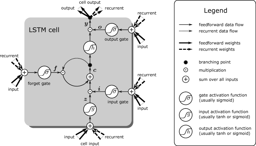
Figure A10: LSTM memory cell without peepholes. $\bm{z}$ is the vector of cell input activations, $\bm{i}$ is the vector of input gate activations, $\bm{f}$ is the vector of forget gate activations, $\bm{c}$ is the vector of memory cell states, $\bm{o}$ is the vector of output gate activations, and $\bm{y}$ is the vector of cell output activations. The activation functions are $g$ for the cell input, $h$ for the cell state, and $\sigma$ for the gates. Data flow is either “feed-forward” without delay or “recurrent” with an one-step delay. “Input” connections are from the external input to the LSTM network, while “recurrent” connections take inputs from other memory cells and hidden units of the LSTM network with a delay of one time step.

A8.2 LSTM in a Nutshell

The central processing and storage unit for LSTM recurrent networks is the memory cell. As already mentioned, it avoids vanishing gradients and allows for uniform credit assignment. The most commonly used LSTM memory cell architecture in the literature [39, 112] contains forget gates [31, 32] and peephole connections [30]. In our previous work [57, 53], we found that peephole connections are only useful for modeling time series, but not for language, meta-learning, or biological sequences. That peephole connections can be removed without performance decrease, was recently confirmed in a large assessment, where different LSTM architectures have been tested [40]. While LSTM networks are highly successful in various applications, the central memory cell architecture was not modified since 2000 [112]. A memory cell architecture without peepholes is depicted in Figure A10.

In our definition of a LSTM network, all units of one kind are pooled to a vector: $\bm{z}$ is the vector of cell input activations, $\bm{i}$ is the vector of input gate activations, $\bm{f}$ is the vector of forget gate activations, $\bm{c}$ is the vector of memory cell states, $\bm{o}$ is the vector of output gate activations, and $\bm{y}$ is the vector of cell output activations. We assume to have an input sequence, where the input vector at time $t$ is $\bm{x}^{t}$. The matrices $\bm{W}_{\bm{z}}$, $\bm{W}_{\bm{i}}$, $\bm{W}_{\bm{f}}$, and $\bm{W}_{\bm{o}}$ correspond to the weights of the connections between inputs and cell input, input gate, forget gate, and output gate, respectively. The vectors $\bm{b}_{\bm{z}}$, $\bm{b}_{\bm{i}}$, $\bm{b}_{\bm{f}}$, and $\bm{b}_{\bm{o}}$ are the bias vectors of cell input, input gate, forget gate, and output gate, respectively. The activation functions are $g$ for the cell input, $h$ for the cell state, and $\sigma$ for the gates, where these functions are evaluated in a component-wise manner if they are applied to vectors. Typically, either the sigmoid $\frac{1}{1+\exp(-x)}$ or $\tanh$ are used as activation functions. $\odot$ denotes the point-wise multiplication of two vectors. Without peepholes, the LSTM memory cell forward pass rules are (see Figure A10):

$$\bm{z}^{t}\ =\ g\left(\bm{W}_{\bm{z}}\ \bm{x}^{t}\ +\ \bm{b}_{\bm{z}}\right)$$ cell input (A326)

$$\bm{i}^{t}\ =\ \sigma\left(\bm{W}_{\bm{i}}\ \bm{x}^{t}\ +\ \bm{b}_{\bm{i}}\right)$$ input gate (A327)

$$\bm{f}^{t}\ =\ \sigma\left(\bm{W}_{\bm{f}}\ \bm{x}^{t}\ +\ \bm{b}_{\bm{f}}\right)$$ forget gate (A328)

$$\bm{c}^{t}\ =\ \bm{i}^{t}\odot\bm{z}^{t}\ +\ \bm{f}^{t}\odot\bm{c}^{t-1}$$ cell state (A329)

$$\bm{o}^{t}\ =\ \sigma\left(\bm{W}_{\bm{o}}\ \bm{x}^{t}\ +\ \bm{b}_{\bm{o}}\right)$$ output gate (A330)

$$\bm{y}^{t}\ =\ \bm{o}^{t}\odot h\left(\bm{c}^{t}\right)$$ cell output (A331)

A8.3 Long-Term Dependencies vs. Uniform Credit Assignment

The LSTM network has been proposed with the aim to learn long-term dependencies in sequences which span over long intervals [55, 56, 50, 51]. However, besides extracting long-term dependencies, LSTM memory cells have another, even more important, advantage in sequence learning: as already described in the early 1990s, LSTM memory cells allow for uniform credit assignment, that is, the propagation of errors back to inputs without scaling them [49]. For uniform credit assignment of current LSTM architectures, the forget gate $\bm{f}$ must be one or close to one. A memory cell without an input gate $\bm{i}$ just sums up all the squashed inputs it receives during scanning the input sequence. Thus, such a memory cell is equivalent to a unit that sees all sequence elements at the same time, as has been shown via the “Ersatzschaltbild” [49]. If an output error occurs only at the end of the sequence, such a memory cell, via backpropagation, supplies the same delta error at the cell input unit $\bm{z}$ at every time step. Thus, all inputs obtain the same credit for producing the correct output and are treated on an equal level and, consequently, the incoming weights to a memory cell are adjusted by using the same delta error at the input unit $\bm{z}$.

In contrast to LSTM memory cells, standard recurrent networks scale the delta error and assign different credit to different inputs. The more recent the input, the more credit it obtains. The first inputs of the sequence are hidden from the final states of the recurrent network. In many learning tasks, however, important information is distributed over the entire length of the sequence and can even occur at the very beginning. For example, in language- and text-related tasks, the first words are often important for the meaning of a sentence. If the credit assignment is not uniform along the input sequence, then learning is very limited. Learning would start by trying to improve the prediction solely by using the most recent inputs. Therefore, the solutions that can be found are restricted to those that can be constructed if the last inputs are considered first. Thus, only those solutions are found that are accessible by gradient descent from regions in the parameter space that only use the most recent input information. In general, these limitations lead to sub-optimal solutions, since learning gets trapped in local optima. Typically, these local optima correspond to solutions which efficiently exploit the most recent information in the input sequence, while information way back in the past is neglected.

A8.4 Special LSTM Architectures for contribution Analysis

A8.4.1 LSTM for Integrated Gradients

For Integrated Gradients contribution analysis with LSTM, we make following assumptions:

1. $\bm{f}^{t}=1$ for all $t$. That is the forget gate is always 1 and nothing is forgotten. We assume uniform credit assignment, which is ensured by the forget gate set to one.

2. $\bm{o}^{t}=1$ for all $t$. That is the output gate is always 1 and nothing is forgotten.

3. We set $h=a_{h}\tanh$ with $a_{h}=1,2,4$.

4. We set $g=a_{g}\tanh$ with $a_{g}=1,2,4$.

5. The cell input gate $\bm{z}$ is only connected to the input but not to other memory cells. $\bm{W}_{\bm{z}}$ has only connections to the input.

6. The input gate $\bm{i}$ is not connected to the input, that is, $\bm{W}_{\bm{i}}$ has only connections to other memory cells. This ensures that LRP assigns relevance only via $\bm{z}$ to the input.

7. The input gate $\bm{i}$ has a negative bias, that is, $\bm{b}_{\bm{i}}<0$. The negative bias reduces the drift effect, that is, the memory content $\bm{c}$ either increases or decreases over time. Typical values are $\bm{b}_{\bm{i}}=-1,-2,-3,-4,-5$.

8. The memory cell content is initialized with zero at time $t=0$, that is, $\bm{c}^{0}=0$.

The resulting LSTM forward pass rules for Integrated Gradients are:

$$\bm{z}^{t}\ =\ a_{g}\ \sigma\left(\bm{W}_{\bm{z}}\ \bm{x}^{t}\ +\ \bm{b}_{\bm{z}}\right)$$ cell input (A332)

$$\bm{i}^{t}\ =\ \sigma\left(\bm{W}_{\bm{i}}\ \bm{x}^{t}\ +\ \bm{b}_{\bm{i}}\right)$$ input gate (A333)

$$\bm{c}^{t}\ =\ \bm{i}^{t}\ \odot\ \bm{z}^{t}\ +\ \bm{c}^{t-1}$$ cell state (A334)

$$\bm{y}^{t}\ =\ a_{h}\ \tanh\left(\bm{c}^{t}\right)$$ cell output (A335)

See Figure A11 which depicts these forward pass rules for Integrated Gradients.

Figure A11: LSTM memory cell used for Integrated Gradients (IG). Forget gates and output gates are set to 1 since they can modify all cell inputs at times after they have been observed, which can make the dynamics highly nonlinear.

A8.4.2 LSTM for LRP

LRP has already been used for LSTM in order to identify important terms in sentiment analysis [1]. In texts, positive and negative terms with respect to the topic could be identified.

For LRP contribution analysis with LSTM, we make following assumptions:

1. $\bm{f}^{t}=1$ for all $t$. That is the forget gate is always 1 and nothing is forgotten. We assume uniform credit assignment, which is ensured by the forget gate set to one.

2. $g>0$, that is, $g$ is positive. For example we can use a sigmoid $\sigma(x)=a_{g}\frac{1}{1+\exp(-x)}$: $g(x)=a_{g}\sigma(x)$, with $a_{g}=2,3,4$. Methods like LRP have problems with negative contributions which cancel with positive contributions [84]. With a positive $g$ all contributions are positive. The cell input $\bm{z}$ (the function $g$) has a negative bias, that is, $\bm{b}_{\bm{z}}<0$. This is important to avoid the drift effect. The drift effect is that the memory content only gets positive contributions which lead to an increase of $\bm{c}$ over time. Typical values are $\bm{b}_{\bm{z}}=-1,-2,-3,-4,-5$.

3. We want to ensure that $h(0)=0$. If the memory content is zero then nothing is transferred to the next layer. Therefore we set $h=a_{h}\tanh$ with $a_{h}=1,2,4$.

4. The cell input gate $\bm{z}$ is only connected to the input but not to other memory cells. $\bm{W}_{\bm{z}}$ has only connections to the input. This ensures that LRP assigns relevance $\bm{z}$ to the input and $\bm{z}$ is not disturbed by redistributing relevance to the network.

5. The input gate $\bm{i}$ is not connected to the input, that is, $\bm{W}_{\bm{i}}$ has only connections to other memory cells. This ensures that LRP assigns relevance only via $\bm{z}$ to the input.

6. The output gate $\bm{o}$ is not connected to the input, that is, $\bm{W}_{\bm{o}}$ has only connections to other memory cells. This ensures that LRP assigns relevance only via $\bm{z}$ to the input.

7. The input gate $\bm{i}$ has a negative bias, that is, $\bm{b}_{\bm{i}}<0$. Like with the cell input the negative bias avoids the drift effect. Typical values are $\bm{b}_{\bm{i}}=-1,-2,-3,-4$.

8. The output gate $\bm{o}$ may also have a negative bias, that is, $\bm{b}_{\bm{o}}<0$. This allows to bring in different memory cells at different time points. It is related to resource allocation.

9. The memory cell content is initialized with zero at time $t=0$, that is, $\bm{c}^{0}=0$. The memory cell content $\bm{c}^{t}$ is non-negative $\bm{c}^{t}\geqslant 0$ since $\bm{z}\geqslant 0$ and $\bm{i}\geqslant 0$.

The resulting LSTM forward pass rules for LRP are:

$$\bm{z}^{t}\ =\ a_{g}\ \sigma\left(\bm{W}_{\bm{z}}\ \bm{x}^{t}\ +\ \bm{b}_{\bm{z}}\right)$$ cell input (A336)

$$\bm{i}^{t}\ =\ \sigma\left(\bm{W}_{\bm{i}}\ \bm{x}^{t}\ +\ \bm{b}_{\bm{i}}\right)$$ input gate (A337)

$$\bm{c}^{t}\ =\ \bm{i}^{t}\ \odot\ \bm{z}^{t}\ +\ \bm{c}^{t-1}$$ cell state (A338)

$$\bm{o}^{t}\ =\ \sigma\left(\bm{W}_{\bm{o}}\ \bm{x}^{t}\ +\ \bm{b}_{\bm{o}}\right)$$ output gate (A339)

$$\bm{y}^{t}\ =\ \bm{o}^{t}\ \odot\ a_{h}\ \tanh\left(\bm{c}^{t}\right)$$ cell output (A340)

See Figure A12 which depicts these forward pass rules for LRP. However, gates may be used while no relevance is given to them which may lead to inconsistencies.

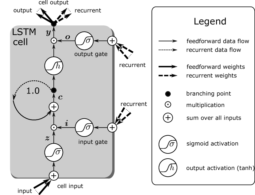
Figure A12: LSTM memory cell used for Layer-Wise Relevance Propagation (LRP). $\bm{z}$ is the vector of cell input activations, $\bm{i}$ is the vector of input gate activations, $\bm{c}$ is the vector of memory cell states, $\bm{o}$ is the vector of output gate activations, and $\bm{y}$ is the vector of cell output activations. The activation functions are the sigmoid $\sigma(x)=a_{g}\frac{1}{1+\exp(-x)}$ and the cell state activation $h(x)=a_{h}\tanh(x)$. Data flow is either “feed-forward” without delay or “recurrent” with an one-step delay. External input reaches the LSTM network only via the cell input $\bm{z}$. All gates only receive recurrent input, that is, from other memory cells.

LRP and Contribution Propagation for LSTM.

We analyze Layer-wise Relevance Propagation (LRP) and Contribution Propagation for LSTM networks. A single memory cell can be described by:

$$c^{t}\ =\ i^{t}\ z^{t}\ +\ c^{t-1}\ .$$ (A341)

Here we treat $i^{t}$ like a weight for $z^{t}$ and $c^{t-1}$ has weight 1.

For positive values of $i^{t}$, $z^{t}$, and $c^{t-1}$, both LRP and contribution propagation leads to

$$R_{c^{t}\leftarrow y^{t}}\ =\ R_{y^{t}}$$ (A342)

$$R_{c^{t}}\ =\ R_{c^{t}\leftarrow c^{t+1}}\ +\ R_{c^{t}\leftarrow y^{t}}$$ (A343)

$$R_{c^{t-1}\leftarrow c^{t}}\ =\ \frac{c^{t-1}}{c^{t}}\ R_{c^{t}}$$ (A344)

$$R_{z^{t}\leftarrow c^{t}}\ =\ \frac{i^{t}\ z^{t}}{c^{t}}\ R_{c^{t}}\ .$$ (A345)

Since we predict only at the last step $t=T$, we have $R_{y^{t}}=0$ for $t<T$. For $t=T$ we obtain $R_{c^{T}}=R_{y^{T}}$, since $R_{c^{T}\leftarrow c^{T+1}}=0$.

We obtain for $t=1\ldots T$:

$$R_{c^{T}}\ =\ R_{y^{T}}$$ (A346)

$$R_{c^{t-1}}\ =\ \frac{c^{t-1}}{c^{t}}\ R_{c^{t}}$$ (A347)

which gives

$$R_{c^{t}}\ =\ R_{y^{T}}\ \prod_{\tau=t+1}^{T}\frac{c^{\tau-1}}{c^{\tau}}\ =\ \frac{c^{t}}{c^{T}}\ R_{y^{T}}$$ (A348)

and consequently as $c^{0}=0$ we obtain

$$R_{c^{0}}\ =\ 0\ ,$$ (A349)

$$R_{z^{t}}\ =\ \frac{i^{t}\ z^{t}}{c^{T}}\ R_{y^{T}}\ .$$ (A350)

Since we assume $c^{0}=0$, we have

$$c^{T}\ =\ \sum_{t=1}^{T}i^{t}\ z^{t}$$ (A351)

and therefore

$$R_{z^{t}}\ =\ \frac{i^{t}\ z^{t}}{\sum_{\tau=1}^{T}i^{\tau}\ z^{\tau}}\ R_{y^{T}}\ .$$ (A352)

Therefore the relevance $R_{y^{T}}$ is distributed across the inputs $z^{t}$ for $t=1\ldots T-1$, where input $z^{t}$ obtains relevance $R_{z^{t}}$.

A8.4.3 LSTM for Nondecreasing Memory Cells

contribution analysis is made simpler if memory cells are nondecreasing since the contribution of each input to each memory cells is well defined. The problem that a negative and a positive input cancels each other is avoided. For nondecreasing memory cells and contribution analysis with LSTM, we make following assumptions:

1. $\bm{f}^{t}=1$ for all $t$. That is the forget gate is always 1 and nothing is forgotten. We assume uniform credit assignment, which is ensured by the forget gate set to one.

2. $g>0$, that is, $g$ is positive. For example we can use a sigmoid $\sigma(x)=a_{g}\frac{1}{1+\exp(-x)}$: $g(x)=a_{g}\sigma(x)$, with $a_{g}=2,3,4$. With a positive $g$ all contributions are positive. The cell input $\bm{z}$ (the function $g$) has a negative bias, that is, $\bm{b}_{\bm{z}}<0$. This is important to avoid the drift effect. The drift effect is that the memory content only gets positive contributions which lead to an increase of $\bm{c}$ over time. Typical values are $\bm{b}_{\bm{z}}=-1,-2,-3,-4,-5$.

3. We want to ensure that $h(0)=0$. If the memory content is zero then nothing is transferred to the next layer. Therefore we set $h=a_{h}\tanh$ with $a_{h}=1,2,4$.

4. The cell input gate $\bm{z}$ is only connected to the input but not to other memory cells. $\bm{W}_{\bm{z}}$ has only connections to the input.

5. The input gate $\bm{i}$ is not connected to the input, that is, $\bm{W}_{\bm{i}}$ has only connections to other memory cells.

6. The output gate $\bm{o}$ is not connected to the input, that is, $\bm{W}_{\bm{o}}$ has only connections to other memory cells.

7. The input gate $\bm{i}$ has a negative bias, that is, $\bm{b}_{\bm{i}}<0$. Like with the cell input the negative bias avoids the drift effect. Typical values are $\bm{b}_{\bm{i}}=-1,-2,-3,-4$.

8. The output gate $\bm{o}$ may also have a negative bias, that is, $\bm{b}_{\bm{o}}<0$. This allows to bring in different memory cells at different time points. It is related to resource allocation.

9. The memory cell content is initialized with zero at time $t=0$, that is, $\bm{c}^{0}=0$. We ensured via the architecture that $\bm{c}^{t}\geqslant 0$ and $\bm{c}^{t+1}\geqslant\bm{c}^{t}$, that is, the memory cells are positive and nondecreasing.

The resulting LSTM forward pass rules for nondecreasing memory cells are:

$$\bm{z}^{t}\ =\ a_{g}\ \sigma\left(\bm{W}_{\bm{z}}\ \bm{x}^{t}\ +\ \bm{b}_{\bm{z}}\right)$$ cell input (A353)

$$\bm{i}^{t}\ =\ \sigma\left(\bm{W}_{\bm{i}}\ \bm{x}^{t}\ +\ \bm{b}_{\bm{i}}\right)$$ input gate (A354)

$$\bm{c}^{t}\ =\ \bm{i}^{t}\ \odot\ \bm{z}^{t}\ +\ \bm{c}^{t-1}$$ cell state (A355)

$$\bm{o}^{t}\ =\ \sigma\left(\bm{W}_{\bm{o}}\ \bm{x}^{t}\ +\ \bm{b}_{\bm{o}}\right)$$ output gate (A356)

$$\bm{y}^{t}\ =\ \bm{o}^{t}\ \odot\ a_{h}\ \tanh\left(\bm{c}^{t}\right)$$ cell output (A357)

See Figure A13 for a LSTM memory cell that is nondecreasing.

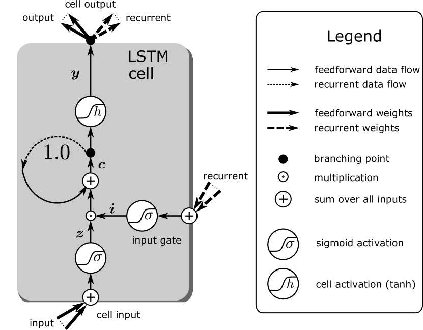
Figure A13: A nondecreasing LSTM memory cell.

A8.4.4 LSTM without Gates

The most simple LSTM architecture for contribution analysis does not use any gates. Therefore complex dynamics that have to be treated in the contribution analysis are avoided. For LSTM without gates, we make following assumptions:

1. $\bm{f}^{t}=1$ for all $t$. That is the forget gate is always 1 and nothing is forgotten.

2. $\bm{o}^{t}=1$ for all $t$. That is the output gate is always 1.

3. $\bm{i}^{t}=1$ for all $t$. That is the input gate is always 1.

4. $g>0$, that is, $g$ is positive. For example we can use a sigmoid $\sigma(x)=a_{g}\frac{1}{1+\exp(-x)}$: $g(x)=a_{g}\sigma(x)$, with $a_{g}=2,3,4$. With a positive $g$ all contributions are positive. The cell input $\bm{z}$ (the function $g$) has a negative bias, that is, $\bm{b}_{\bm{z}}<0$. This is important to avoid the drift effect. The drift effect is that the memory content only gets positive contributions which lead to an increase of $\bm{c}$ over time. Typical values are $\bm{b}_{\bm{z}}=-1,-2,-3,-4,-5$.

5. We want to ensure that $h(0)=0$. If the memory content is zero then nothing is transferred to the next layer. Therefore we set $h=a_{h}\tanh$ with $a_{h}=1,2,4$.

6. The memory cell content is initialized with zero at time $t=0$, that is, $\bm{c}^{0}=0$.

The resulting LSTM forward pass rules are:

$$\bm{z}^{t}\ =\ a_{g}\ \sigma\left(\bm{W}_{\bm{z}}\ \bm{x}^{t}\ +\ \bm{b}_{\bm{z}}\right)$$ cell input (A358)

$$\bm{c}^{t}\ =\ \bm{z}^{t}\ +\ \bm{c}^{t-1}$$ cell state (A359)

$$\bm{y}^{t}\ =\ a_{h}\ \tanh\left(\bm{c}^{t}\right)$$ cell output (A360)

See Figure A14 for a LSTM memory cell without gates which perfectly distributes the relevance across the input.

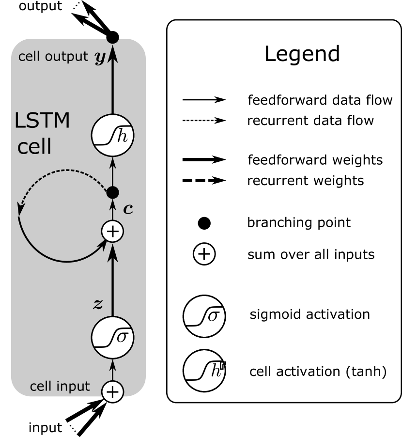
Figure A14: LSTM memory cell without gates.

Appendix A9 Contribution Analysis

A9.1 Difference of Consecutive Predictions for Sequences

General Approach.

The idea is to assess the information gain that is induced by an input at a particular time step. This information gain is used for predicting the target at sequence end by determining the change in prediction. The input to a recurrent neural network is the sequence $\bm{x}=(x_{1},\ldots,x_{d})$ with target $y_{d}$, which is only given at sequence end. The prefix sequence $\bm{x}_{t}$ of length $t\leqslant d$ is $\bm{x}_{t}=(x_{1},\ldots,x_{t})$. $F$ predicts the target $y_{d}$ at every time step $t$:

$$F(\bm{x}_{t})\ =\ y_{d}\ .$$ (A361)

We can define the decomposition of $F$ through contributions at different time steps

$$h_{0}\ =\ F(\bm{x}_{0})\ ,$$ (A362)

$$h_{t}\ =\ F(\bm{x}_{t})\ -\ F(\bm{x}_{t-1})\ \text{ for }t>0\ ,$$ (A363)

where $F(\bm{x}_{0})$ is a predefined constant. We have

$$F(\bm{x}_{t})\ =\ \sum_{\tau=0}^{t}h_{\tau}\ .$$ (A364)

We assume a loss function for $F$ that is minimal if $F\equiv F_{\min}$ predicts the expected $y_{d}$

$$F_{\min}(\bm{x}_{t})\ =\ \mathbf{\mathrm{E}}\left[y_{d}\mid\bm{x}_{t}\right]\ .$$ (A365)

Then

$$h_{0}\ =\ \mathbf{\mathrm{E}}\left[y_{d}\right]\ ,$$ (A366)

$$h_{t}\ =\ \mathbf{\mathrm{E}}\left[y_{d}\mid\bm{x}_{t}\right]\ -\ \mathbf{\mathrm{E}}\left[y_{d}\mid\bm{x}_{t-1}\right]\ \text{ for }t>0\ .$$ (A367)

In this case, the contributions are the change in the expectation of the target that will be observed at sequence end. The contribution can be viewed as the information gain in time step $t$ for predicting the target. If we cannot ensure that $F$ predicts the target at every time step, then other contribution analysis methods must be employed. For attributing the prediction of a deep network to its input features several contribution analysis methods have been proposed. We consider Input Zeroing, Integrated Gradients (IG), and Layer-Wise Relevance Propagation (LRP).

Linear Models and Coefficient of Determination.

We consider linear models and the average gain of information about the reward at sequence end if we go one time step further in the input sequence. By adding a variable, that is, another sequence element, the mean squared error (MSE) decreases, which is the amount by which the expectation improves due to new information. But by what amount does the MSE decrease in average? Here, we consider linear models. For linear models we are interested in how much the coefficient of determination increases if we add another variable, that is, if we see another input.

We consider the feature vector $\bm{x}=(x_{1},x_{2},\ldots,x_{k})^{T}$ from which the target $y$ (the reward at sequence end) has to be predicted. We assume to have $n$ pairs $(\bm{x}_{i},y_{i}),1\leqslant i\leqslant n$, as training set. The prediction or estimation of $y_{i}$ from $\bm{x}_{i}$ is $\hat{y}_{i}$ with $\hat{y}_{i}=F(\bm{x}_{i})$. The vector of all training labels is $\bm{y}=(y_{1},\ldots,y_{n})$ and the training feature matrix is $\bm{X}=(\bm{x}_{1},\ldots,\bm{x}_{n})$. We define the mean squared error (MSE) as

$$\mathrm{mse}(\bm{y},\bm{X})\ =\ \frac{1}{n-1}\ \sum_{i=1}^{n}\left(\hat{y}_{i}\ -\ y_{i}\right)^{2}\ .$$ (A368)

The coefficient of determination $R^{2}$ is equal to the correlation between the target $y$ and its prediction $\hat{y}$. $R^{2}$ is given by:

$$R^{2}\ =\ 1\ -\ \frac{\frac{1}{n-1}\ \sum_{i=1}^{n}\left(\hat{y}_{i}\ -\ y_{i}\right)^{2}}{\frac{1}{n-1}\ \sum_{i=1}^{n}\left(y_{i}\ -\ \bar{y}\right)^{2}}\ =\ 1\ -\ \frac{\mathrm{mse}(\bm{y},\bm{X})}{s_{y}^{2}}\ .$$ (A369)

Therefore, $R^{2}$ is one minus the ratio of the mean squared error divided by the mean total sum of squares. $R^{2}$ is a strict monotonically decreasing function of the mean squared error.

We will give a breakdown of the factors that determine how much each variable adds to $R^{2}$ [100, chapter 10.6, p. 263]. The feature vector $\bm{x}$ is expanded by one additional feature $z$: $\bm{w}=(x_{1},x_{2},\ldots,x_{k},z)^{T}=(\bm{x}^{T},z)^{T}$. We want to know the increase in $R^{2}$ due to adding $z$. Therefore, we decompose $\bm{w}$ into $\bm{x}$ and $z$. The difference in coefficients of determination is the difference of the according MSEs divided by the empirical variance of $y$:

$$R^{2}_{y\bm{w}}\ -\ R^{2}_{y\bm{x}}\ =\ \frac{\mathrm{mse}(\bm{y},\bm{W})\ -\ \mathrm{mse}(\bm{y},\bm{X})}{s_{y}^{2}}\ .$$ (A370)

We further need definitions:

• $\bm{x}=(x_{1},x_{2},\ldots,x_{k})^{T}$.

• $\bm{w}=(x_{1},x_{2},\ldots,x_{k},z)^{T}=(\bm{x}^{T},z)^{T}$.

• The sample covariance between $y$ and $x$ is $s_{yx}=\sum_{i=1}^{n}(x_{i}-\bar{x})(y_{i}-\bar{y})/(n-1)$, where $\bar{x}=\sum_{i=1}^{n}x_{i}/n$ and $\bar{y}=\sum_{i=1}^{n}y_{i}/n$ are the sample means. The variance of $x$ is $s_{xx}$ often written as $s_{x}^{2}$, the standard deviation squared: $s_{x}:=\sqrt{s_{xx}}$.

• The correlation between $y$ and $x$ is $r_{yx}=s_{yx}/(s_{x}s_{y})$.

• The covariance matrix $\bm{S}_{xx}$ of a vector $\bm{x}$ is the matrix with entries $[\bm{S}_{xx}]_{ij}=s_{x_{i}x_{j}}$.

• The covariance matrix $\bm{R}_{xx}$ of a vector $\bm{x}$ is the matrix with entries $[\bm{R}_{xx}]_{ij}=r_{x_{i}x_{j}}$.

• The diagonal matrix $\bm{D}_{x}=[\mathrm{diag}(\bm{S}_{xx})]^{1/2}$ has a $i$th diagonal entry $\sqrt{s_{x_{i}}}$ and is the diagonal matrix of standard deviations of the components of $\bm{x}$.

• $R^{2}_{yw}$ is the squared multiple correlation between $y$ and $\bm{w}$.

• $R^{2}_{yx}$ is the squared multiple correlation between $y$ and $\bm{x}$.

• $R^{2}_{zx}=\bm{s}_{zx}^{T}\bm{S}_{xx}^{-1}\bm{s}_{zx}/s_{z}^{2}=\bm{r}_{zx}^{T}\bm{R}_{xx}^{-1}\bm{r}_{zx}$ is the squared multiple correlation between $z$ and $\bm{x}$.

• $r_{yz}$ is the simple correlation between $y$ and $z$: $r_{yz}=s_{yz}/(s_{y}s_{z})$.

• $\bm{r}_{yx}=(r_{yx_{1}},r_{yx_{2}},\ldots,r_{yx_{k}})^{T}=s_{y}^{-1}\bm{D}_{x}^{-1}\bm{S}_{yx}$ is the vector of correlations between $y$ and $\bm{x}$.

• $\bm{r}_{zx}=(r_{zx_{1}},r_{zx_{2}},\ldots,r_{zx_{k}})^{T}=s_{z}^{-1}\bm{D}_{x}^{-1}\bm{S}_{zx}$ is the vector of correlations between $z$ and $\bm{x}$.

• $\hat{\bm{\beta}}^{*}_{zx}=\bm{R}_{xx}^{-1}\bm{r}_{zx}$ is the vector of standardized regression coefficients (beta weights) of $z$ regressed on $\bm{x}$.

• The parameter vector is partitioned into the constant $\beta_{0}$ and $\bm{\beta}_{1}$ via $\bm{\beta}=(\beta_{0},\beta_{1},\ldots,\beta_{m})^{T}=(\beta_{0},\bm{\beta}_{1}^{T})^{T}$. We have for the maximum likelihood estimate

  $$\hat{\beta}_{0}\ =\ \bar{y}\ -\ \bm{s}_{yx}^{T}\bm{S}_{xx}^{-1}\bar{\bm{x}}\ ,$$ (A371)

  $$\hat{\bm{\beta}}_{1}\ =\ \bm{S}_{xx}^{-1}\bm{s}_{yx}\ .$$ (A372)

  The offset $\hat{\beta}_{0}$ guarantees $\bar{\hat{y}}=\bar{y}$, therefore, $\bm{y}^{T}\bar{\bm{y}}=\hat{\bm{y}}^{T}\bar{\bm{y}}$, since $\bar{\bm{y}}=\bar{y}\bm{1}$:

  $$\bar{\hat{y}}\ =\ \frac{1}{n}\ \sum_{i=1}^{n}\hat{y}_{i}\ =\ \frac{1}{n}\ \sum_{i=1}^{n}\big{(}\hat{\beta}_{0}\ +\ \hat{\bm{\beta}}_{1}^{T}\bm{x}_{i}\big{)}$$ (A373)

  $$=\ \bar{y}\ -\ \bm{s}_{yx}^{T}\bm{S}_{xx}^{-1}\bar{\bm{x}}\ +\ \frac{1}{n}\ \sum_{i=1}^{n}\hat{\bm{\beta}}_{1}^{T}\bm{x}_{i}$$

  $$=\ \bar{y}\ -\ \bm{s}_{yx}^{T}\bm{S}_{xx}^{-1}\bar{\bm{x}}\ +\ \bm{s}_{yx}^{T}\bm{S}_{xx}^{-1}\bar{\bm{x}}$$

  $$=\ \bar{y}\ .$$

• The vector of standardized coefficients $\hat{\bm{\beta}}^{*}_{1}$ are

  $$\hat{\bm{\beta}}^{*}_{1}\ =\ \frac{1}{s_{y}}\ \bm{D}_{x}\ \hat{\bm{\beta}}_{1}\ =\ \bm{R}_{xx}^{-1}\ \bm{r}_{yx}\ .$$ (A374)

The next theorem is Theorem 10.6 in Rencher and Schaalje [100] and gives a breakdown of the factors that determine how much each variable adds to $R^{2}$ [100, Chapter 10.6, p. 263].

Theorem 1 (Rencher Theorem 10.6).

The increase in $R^{2}$ due to $z$ can be expressed as

$$R^{2}_{y\bm{w}}\ -\ R^{2}_{y\bm{x}}\ =\ \frac{(\hat{r}_{yz}\ -\ r_{yz})^{2}}{1\ -\ R^{2}_{zx}}\ ,$$ (A375)

where $\hat{r}_{yz}=(\hat{\bm{\beta}}^{*}_{zx})^{T}\bm{r}_{yx}$ is a “predicted” value of $r_{yz}$ based on the relationship of $z$ to the $\bm{x}$’s.

The following equality shows that $\hat{r}_{yz}=(\hat{\bm{\beta}}^{*}_{zx})^{T}\bm{r}_{yx}$ is indeed a prediction of $r_{yz}$:

$$\left(\hat{\bm{\beta}}^{*}_{zx}\right)^{T}\bm{r}_{yx}\ =\ \frac{1}{s_{z}}\ \bm{D}_{x}\ \hat{\bm{\beta}}_{zx}^{T}\frac{1}{s_{y}}\ \bm{D}_{x}^{-1}\bm{s}_{yx}$$ (A376)

$$=\ \frac{1}{s_{z}\ s_{y}}\ \hat{\bm{\beta}}_{zx}^{T}\frac{1}{n-1}\ \sum_{i=1}^{n}(\bm{x}_{i}-\bar{\bm{x}})(y_{i}-\bar{y})$$

$$=\ \frac{1}{s_{z}\ s_{y}}\ \frac{1}{n-1}\ \sum_{i=1}^{n}(\hat{\bm{\beta}}_{zx}^{T}\bm{x}_{i}-\hat{\bm{\beta}}_{zx}^{T}\bar{\bm{x}})(y_{i}-\bar{y})$$

$$=\ \frac{1}{s_{z}\ s_{y}}\ \frac{1}{n-1}\ \sum_{i=1}^{n}(\hat{z_{i}}-\bar{\hat{z}})(y_{i}-\bar{y})$$

$$=\ \frac{1}{s_{z}\ s_{y}}\ \hat{s}_{yz}\ =\ \hat{r}_{yz}\ .$$

If $z$ is orthogonal to $\bm{x}$ (i.e., if $\bm{r}_{zx}=\bm{0}$), then $\hat{\bm{\beta}}^{*}_{zx}=\bm{0}$, which implies that $\hat{r}_{yz}=0$ and $R^{2}_{zx}=0$. In this case, Eq. (A375) can be written as

$$R^{2}_{y\bm{w}}\ -\ R^{2}_{y\bm{x}}\ =\ r_{yz}^{2}\ .$$ (A377)

Consequently, if all $x_{i}$ are independent from each other, then

$$R^{2}_{y\bm{x}}\ =\ \sum_{j=1}^{k}r_{yx_{j}}^{2}\ .$$ (A378)

The contribution of $z$ to $R^{2}$ can either be less than or greater than $r_{yz}$. If the correlation $r_{yz}$ can be predicted from $\bm{x}$, then $\hat{r}_{yz}$ is close to $r_{yz}$ and, therefore, $z$ has contributes less to $R^{2}$ than $r_{yz}^{2}$.

Next, we compute the contribution of $z$ to $R^{2}$ explicitly. The correlation between $y$ and $z$ is

$$r_{yz}\ =\ \frac{1}{s_{z}\ s_{y}}\ \frac{1}{n-1}\ \sum_{i=1}^{n}(z_{i}-\bar{z})(y_{i}-\bar{y})\ =\ \frac{1}{s_{z}\ s_{y}}\ s_{yz}\ .$$ (A379)

We assume that $\bar{z}=\bar{\hat{z}}$. We want to express the information gain using the mean squared error (MSE) $1/(n-1)\sum_{i=1}^{n}(\hat{z_{i}}-z_{i})^{2}$. We define the error $e_{i}:=\hat{z_{i}}-z_{i}$ at sample $i$ with $\bar{e}=\bar{\hat{z}}-\bar{z}=0$. Therefore, the MSE is equal to the empirical variance $s_{e}^{2}=1/(n-1)\sum_{i=1}^{n}e_{i}^{2}$. The correlation $r_{ey}$ between the target $y$ and the error $e$ is

$$r_{ey}\ =\ \frac{1}{s_{y}\ s_{e}}\ \frac{1}{n-1}\ \sum_{i=1}^{n}(e_{i}\ -\ \bar{e})\ (y_{i}-\bar{y})\ .$$ (A380)

Using Eq. (A376) and Eq. (A379), we can express the difference between the estimate $\hat{r}_{yz}$ and the true correlation $r_{yz}$ by:

$$\hat{r}_{yz}\ -\ r_{yz}\ =\ \frac{1}{s_{z}\ s_{y}}\ \frac{1}{n-1}\ \sum_{i=1}^{n}(\hat{z_{i}}-\bar{\hat{z}})(y_{i}-\bar{y})\ -\ \frac{1}{s_{z}\ s_{y}}\ \frac{1}{n-1}\ \sum_{i=1}^{n}(z_{i}-\bar{z})(y_{i}-\bar{y})$$ (A381)

$$=\ \frac{1}{s_{z}\ s_{y}}\ \frac{1}{n-1}\ \sum_{i=1}^{n}(\hat{z_{i}}-z_{i})(y_{i}-\bar{y})\ .$$

The information gain can now be expressed by the correlation $r_{ey}$ between the target $y$ and the error $e$:

$$R^{2}_{y\bm{w}}\ -\ R^{2}_{y\bm{x}}\ =\ \frac{(\hat{r}_{yz}\ -\ r_{yz})^{2}}{1\ -\ R^{2}_{zx}}\ =\ \frac{\frac{1}{s_{z}^{2}\ s_{y}^{2}}\ \frac{1}{(n-1)^{2}}\ \left(\sum_{i=1}^{n}(\hat{z_{i}}-z_{i})(y_{i}-\bar{y})\right)^{2}}{\frac{\frac{1}{n-1}\ \sum_{i=1}^{n}\left(\hat{z}_{i}\ -\ z_{i}\right)^{2}}{\frac{1}{n-1}\ \sum_{i=1}^{n}\left(z_{i}\ -\ \bar{z}\right)^{2}}}$$ (A382)

$$=\ \frac{\frac{1}{s_{y}^{2}}\ \frac{1}{(n-1)^{2}}\ \left(\sum_{i=1}^{n}(\hat{z_{i}}-z_{i})(y_{i}-\bar{y})\right)^{2}}{\frac{1}{n-1}\ \sum_{i=1}^{n}\left(\hat{z}_{i}\ -\ z_{i}\right)^{2}}$$

$$=\ r_{ey}^{2}\ .$$

The information gain is the squared correlation $r_{ey}^{2}$ between the target $y$ and the error $e$. The information gain is the information in $z$ about $y$, which is not contained in $\bm{x}$.

A9.2 Input Zeroing

The simplest contribution analysis method is Input Zeroing, where just an input is set to zero to determine its contribution to the output. Input Zeroing sets a particular input $x_{i}$ to zero and then computes the network’s output. For the original input $\bm{x}=(x_{1},\ldots,x_{d})$ and the input with $x_{i}=0$, i.e. $\tilde{\bm{x}}_{i}=(x_{1},\ldots,x_{i-1},0,x_{i+1},\ldots,x_{d})$, we compute $\Delta x_{i}=F(\bm{x})\ -\ F(\tilde{\bm{x}}_{i})$ to obtain the contribution of $x_{i}$. We obtain for the difference of $F(\bm{x})$ to the baseline of average zeroing $\frac{1}{d}\sum_{i=1}^{d}F(\tilde{\bm{x}}_{i})$:

$$F(\bm{x})\ -\ \frac{1}{d}\ \sum_{i=1}^{d}F(\tilde{\bm{x}}_{i})\ =\ \frac{1}{d}\ \sum_{i=1}^{d}\Delta x_{i}\ .$$ (A383)

The problem is that the $F(\tilde{\bm{x}}_{i})$ have to be computed $d$-times, that is, for each input component zeroed out.

Input Zeroing does not recognize redundant inputs, i.e. each one of the inputs is sufficient to produce the output but if all inputs are missing at the same time then the output changes. In contrast, Integrated Gradients (IG) and Layer-Wise Relevance Propagation (LRP) detect the relevance of an input even if it is redundant.

A9.3 Integrated Gradients

Integrated gradients is a recently introduced method [125]. Integrated gradients decomposes the difference $F(\bm{x})-F(\tilde{\bm{x}})$ between the network output $F(\bm{x})$ and a baseline $F(\tilde{\bm{x}})$:

$$F(\bm{x})\ -\ F(\tilde{\bm{x}})\ =\ \sum_{i=1}^{d}(x_{i}\ -\ \tilde{x}_{i})\ \int_{t=0}^{1}\frac{\partial F}{\partial x_{i}}(\tilde{\bm{x}}+t(\bm{x}-\tilde{\bm{x}}))\,\mathrm{d}t$$ (A384)

$$\approx\ \sum_{i=1}^{d}(x_{i}\ -\ \tilde{x}_{i})\ \frac{1}{m}\ \sum_{k=1}^{m}\frac{\partial F}{\partial x_{i}}(\tilde{\bm{x}}+(k/m)(\bm{x}-\tilde{\bm{x}}))\ .$$

In contrast to previous approaches, we have $F$ and its derivative to evaluate only $m$-times, where $m<d$.

The equality can be seen if we define $\bm{h}=\bm{x}-\tilde{\bm{x}}$ and

$$\begin{cases}g:[0,1]\to\mathbb{R}\\ g(t)=F(\bm{x}+t\bm{h})\ .\end{cases}$$ (A385)

Consequently, we have

$$F(\bm{x}+\bm{h})-F(\bm{x})\ =\ g(1)-g(0)\ =\ \int_{0}^{1}g^{\prime}(t)\,\mathrm{d}t$$ (A386)

$$=\ \int_{0}^{1}\left(\sum_{i=1}^{d}\ \frac{\partial F}{\partial x_{i}}(\bm{x}+t\bm{h})\ h_{i}\right)\,\mathrm{d}t\ =\ \sum_{i=1}^{d}\ \left(\int_{0}^{1}\frac{\partial F}{\partial x_{i}}(\bm{x}+t\bm{h})\,\mathrm{d}t\right)\ h_{i}\ .$$ (A387)

For the final reward decomposition, we obtain

$$F(\bm{x})\ =\ \sum_{i=1}^{d}\left((x_{i}\ -\ \tilde{x}_{i})\ \frac{1}{m}\ \sum_{k=1}^{m}\frac{\partial F}{\partial x_{i}}(\tilde{\bm{x}}+(k/m)(\bm{x}-\tilde{\bm{x}}))\ +\ \frac{1}{d}\ F(\tilde{\bm{x}})\right)\ .$$ (A388)

A9.4 Layer-Wise Relevance Propagation

Layer-Wise Relevance Propagation (LRP) [3] has been introduced to interpret machine learning models. LRP is an extension of the contribution-propagation algorithm [71] based on the contribution approach [94]. Recently “excitation backprop” was proposed [147], which is like LPR but uses only positive weights and shifts the activation function to have non-negative values. Both algorithms assign a relevance or importance value to each node of a neural network which describes how much it contributed to generating the network output. The relevance or importance is recursively propagated back: A neuron is important to the network output if it has been important to its parents, and its parents have been important to the network output. LRP moves through a neural network like backpropagation: it starts at the output, redistributes the relevance scores of one layer to the previous layer until the input layer is reached. The redistribution procedure satisfies a local relevance conservation principle. All relevance values that a node obtains from its parents will be redistributed to its children. This is analog to Kirchhoff’s first law for the conservation of electric charge or the continuity equation in physics for transportation in general form. LRP has been used for deep neural networks (DNN) [84] and for recurrent neural networks like LSTM [1].

We consider a neural network with activation $x_{i}$ for neuron $i$. The weight from neuron $l$ to neuron $i$ is denoted by $w_{il}$. The activation function is $g$ and $\mathrm{net}_{i}$ is the netinput to neuron $i$ with bias $b_{i}$. We have following forward propagation rules:

$$\mathrm{net}_{i}\ =\ \sum_{l}w_{il}\ x_{l}\ ,$$ (A389)

$$x_{i}\ =\ f_{i}(\mathrm{net}_{i})\ =\ g(\mathrm{net}_{i}+b_{i})\ .$$ (A390)

Let $R_{i}$ be the relevance for neuron $i$ and $R_{i\leftarrow k}$ the share of relevance $R_{k}$ that flows from neuron $k$ in the higher layer to neuron $i$ in the lower layer. The parameter $z_{ik}$ is a weighting for the share of $R_{k}$ of neuron $k$ that flows to neuron $i$. We define $R_{i\leftarrow k}$ as

$$R_{i\leftarrow k}\ =\ \frac{z_{ik}}{\sum_{l}z_{lk}}\ R_{k}\ .$$ (A391)

The relative contributions $z_{ik}$ are previously defined as [3, 84, 1]:

$$z_{ik}\ =\ w_{ik}\ x_{k}\ .$$ (A392)

Here, $z_{ik}$ is the contribution of $x_{k}$ to the netinput value $\mathrm{net}_{i}$. If neuron $k$ is removed from the network, then $z_{ik}$ will be the difference to the original $\mathrm{net}_{i}$.

The relevance $R_{i}$ of neuron $i$ is the sum of relevances it obtains from its parents $k$ from a layer above:

$$R_{i}\ =\ \sum_{k}R_{i\leftarrow k}\ .$$ (A393)

Furthermore, a unit $k$ passes on all its relevance $R_{k}$ to its children, which are units $i$ of the layer below:

$$R_{k}\ =\ \sum_{i}R_{i\leftarrow k}\ .$$ (A394)

It follows the conservation of relevance. The sum of relevances $R_{k}$ of units $k$ in a layer is equal to the sum of relevances $R_{i}$ of units $i$ of a layer below:

$$\sum_{k}R_{k}\ =\ \sum_{k}\ \sum_{i}R_{i\leftarrow k}\ =\ \sum_{i}\ \sum_{k}R_{i\leftarrow k}\ =\ \sum_{i}R_{i}\ .$$ (A395)

The scalar output $g(\bm{x})$ of a neural network with input $\bm{x}=(x_{1},\ldots,x_{d})$ is considered as relevance $R$ which is decomposed into contributions $R_{i}$ of the inputs $x_{i}$:

$$\sum_{i}R_{i}\ =\ R\ =\ g(\bm{x})\ .$$ (A396)

The decomposition is valid for recurrent neural networks, where the relevance at the output is distributed across the sequence elements of the input sequence.

A9.4.1 New Variants of LRP

An alternative definition of $z_{ik}$ is

$$z_{ik}\ =\ w_{ik}\ (x_{k}\ -\ \bar{x}_{k})\ ,$$ (A397)

where $\bar{x}_{k}$ is the mean of $x_{k}$ across samples. Therefore, $(x_{k}\ -\ \bar{x}_{k})$ is the contribution of the actual sample to the variance of $x_{k}$. This in turn is related to the information carried by $x_{k}$. Here, $z_{ik}$ is the contribution of $x_{k}$ to the variance of $\mathrm{net}_{i}$. However, we can have negative values of $(x_{k}\ -\ \bar{x}_{k})$ which may lead to negative contributions even if the weights are positive.

Another alternative definition of $z_{ik}$ is

$$z_{ik}\ =\ f_{i}(\mathrm{net}_{i})\ -\ f_{i}(\mathrm{net}_{i}\ -\ w_{ik}\ x_{k})\ .$$ (A398)

Here, $z_{ik}$ is the contribution of $x_{k}$ to the activation value $x_{i}=f_{i}(\mathrm{net}_{i})$. If neuron $k$ is removed from the network, then $z_{ik}$ will be the difference to the original $x_{i}$. If $f_{i}$ is strict monotone increasing and $x_{k}>0$, then positive weights $w_{ik}$ will lead to positive values and negative weights $w_{ik}$ to negative values.

Preferred Solution:
A definition of $z_{ik}$ is

$$z_{ik}\ =\ w_{ik}\ (x_{k}\ -\ x_{\min})\ ,$$ (A399)

where $x_{\min}$ is the minimum of $x_{k}$ either across samples (mini-batch) or across time steps. The difference $(x_{k}-x_{\min})$ is always positive. Using this definition, activation functions with negative values are possible, like for excitation backprop [147]. The minimal value is considered as default off-set, which can be included into the bias.

A9.4.2 LRP for Products

Here we define relevance propagation for products of two units. We assume that $z=x_{1}x_{2}$ with $x_{1}>0$ and $x_{2}>0$. We view $x_{1}$ and $x_{2}$ as units of a layer below the layer in which $z$ is located. Consequently, $R_{z}$ has to be divided between $x_{1}$ and $x_{2}$, which gives the conservation rule

$$R_{z}\ =\ R_{x_{1}\leftarrow z}\ +\ R_{x_{2}\leftarrow z}\ .$$ (A400)

Alternative 1:

$$R_{x_{1}\leftarrow z}\ =\ 0.5\ R_{z}$$ (A401)

$$R_{x_{2}\leftarrow z}\ =\ 0.5\ R_{z}\ .$$ (A402)

The relevance is equally distributed.

Preferred Solution:
Alternative 2: The contributions according to the deep Taylor decomposition around $(a,a)$ are

$$\frac{\partial z}{\partial x_{1}}\bigg{\rvert}_{(a,a)}\ (x_{1}-a)\ =\ (x_{1}-a)\ a\ ,$$ (A403)

$$\frac{\partial z}{\partial x_{2}}\bigg{\rvert}_{(a,a)}\ (x_{2}-a)\ =\ a\ (x_{2}-a)\ .$$ (A404)

We compute the relative contributions:

$$\frac{(x_{1}-a)\ a}{(x_{1}-a)\ a\ +\ a\ (x_{2}-a)}\ =\ \frac{x_{1}-a}{(x_{1}\ +\ x_{2}\ -\ 2\ a)}\ ,$$ (A405)

$$\frac{(x_{2}-a)\ a}{(x_{1}-a)\ a\ +\ a\ (x_{2}-a)}\ =\ \frac{x_{2}-a}{(x_{1}\ +\ x_{2}\ -\ 2\ a)}\ .$$ (A406)

For $\lim_{a\to 0}$ we obtain $x_{1}/(x_{1}+x_{2})$ and $x_{2}/(x_{1}+x_{2})$ as contributions.

We use this idea but scale $x_{1}$ and $x_{2}$ to the range $[0,1]$:

$$R_{x_{1}\leftarrow z}\ =\ \frac{\frac{x_{1}-x_{\min}}{x_{\max}-x_{\min}}}{\frac{x_{1}-x_{\min}}{x_{\max}-x_{\min}}\ +\ \frac{x_{2}-x_{\min}}{x_{\max}-x_{\min}}}\ R_{z}$$ (A407)

$$R_{x_{2}\leftarrow z}\ =\ \frac{\frac{x_{2}-x_{\min}}{x_{\max}-x_{\min}}}{\frac{x_{1}-x_{\min}}{x_{\max}-x_{\min}}\ +\ \frac{x_{2}-x_{\min}}{x_{\max}-x_{\min}}}\ R_{z}\ .$$ (A408)

The relevance is distributed according to how close the maximal value is achieved and how far away it is from the minimal value.

Alternative 3:

$$R_{x_{1}\leftarrow z}\ =\ \frac{\ln\left(1-\frac{x_{1}-x_{\min}}{x_{\max}-x_{\min}}\right)}{\ln\left(1-\frac{x_{1}-x_{\min}}{x_{\max}-x_{\min}}\right)\ +\ \ln\left(1-\frac{x_{2}-x_{\min}}{x_{\max}-x_{\min}}\right)}\ R_{z}$$ (A409)

$$R_{x_{2}\leftarrow z}\ =\ \frac{\ln\left(1-\frac{x_{2}-x_{\min}}{x_{\max}-x_{\min}}\right)}{\ln\left(1-\frac{x_{1}-x_{\min}}{x_{\max}-x_{\min}}\right)\ +\ \ln\left(1-\frac{x_{2}-x_{\min}}{x_{\max}-x_{\min}}\right)}\ R_{z}\ .$$ (A410)

All $\ln$-values are negative, therefore the fraction in front of $R_{z}$ is positive. $x_{1}=x_{\min}$ leads to a zero relevance for $x_{1}$. The ratio of the relevance for $x_{1}$ increases to 1 when $x_{1}$ approaches $x_{\max}$. The relevance is distributed according to how close the maximal value is achieved. We assume that the maximal value is a saturating value, therefore we use $\ln$, the natural logarithm.

A9.5 Variance Considerations for contribution Analysis

We are interested how the redistributed reward affects the variance of the estimators. We consider (A) the difference of consecutive predictions is the redistributed reward, (B) integrated gradients (IG), and (C) layer-wise relevance propagation (LRP).

For (A) the difference of consecutive predictions is the redistributed reward, all variance is moved to the final correction. However imperfect $g$ and variance cannot be distinguished.

For (B) integrated gradients (IG) the redistributed rewards depend on future values. Therefore the variance can even be larger than in the original MDP.

For (C) layer-wise relevance propagation (LRP) the variance is propagated back without decreasing or increasing if the actual return is used as relevance. If the prediction is used as relevance and a final correction is used then the variance is moved to the final prediction but new variance is injected since rewards depend on the future path.

Appendix A10 Reproducibility Checklist

We followed the reproducibility checklist [92] and point to relevant sections.

For all models and algorithms presented, check if you include:

• A clear description of the mathematical setting, algorithm, and/or model.

  Description of mathematical settings starts at paragraph  MDP Definitions and Return-Equivalent Sequence-Markov Decision Processes (SDPs)..

  Description of novel learning algorithms starts at paragraph Novel Learning Algorithms Based on Reward Redistributions..

• An analysis of the complexity (time, space, sample size) of any algorithm.

  Plots in Figure 1 show the number of episodes, i.e. the sample size, which are needed for convergence to the optimal policies. They are evaluated for different algorithms and delays in all artificial tasks. For Atari games, the number of samples corresponds to the number of game frames. See paragraph Atari Games.. We further present a bias-variance analysis of TD and MC learning in Section A3.1 and Section A3.2 in the appendix.

• A link to a downloadable source code, with specification of all dependencies, including external libraries.

  https://github.com/ml-jku/baselines-rudder

For any theoretical claim, check if you include:

• A statement of the result.

  The main theorems:

  • Theorem 1

  • Theorem 2

  • Theorem 3

  Additional supporting theorems can be found in the proof section of the appendix A2.

• A clear explanation of any assumptions.

  The proof section A2 in the appendix covers all the assumptions for the main theorems.

• A complete proof of the claim.

  Proof of the main theorems are moved to the appendix.

  • Proof of Theorem 1 can be found after Theorem A2 in the appendix.

  • Proof of Theorem 2 can be found after Theorem A4 in the appendix.

  • Proof of Theorem 3 can be found after Theorem A5 in the appendix.

  Proofs for additional theorems can also be found in this appendix.

For all figures and tables that present empirical results, check if you include:

• A complete description of the data collection process, including sample size.

  For artificial tasks the environment descriptions can be found in section Artificial Tasks in the main paper. For Atari games, we use the standard sampling procedures as in OpenAI Gym [18] (description can be found in paragraph Atari Games.).

• A link to a downloadable version of the dataset or simulation environment.

  Link to our repository: https://github.com/ml-jku/rudder

• An explanation of any data that were excluded, description of any pre-processing step

  For Atari games, we use the standard pre-processing described in [80].

• An explanation of how samples were allocated for training / validation / testing.

  For artificial tasks, description of training and evaluation are included in section A4.1 . For Atari games, description of training and evaluation are included Section A4.1.

• The range of hyper-parameters considered, method to select the best hyper-parameter configuration, and specification of all hyper-parameters used to generate results.

  A description can be found at paragraph PPO model. in the appendix.

• The exact number of evaluation runs.

  For artificial tasks evaluation was performed during training runs. See Figure 1. For Atari games see paragraph Atari Games.. We also provide a more detailed description in Section A4.1 and Section A4.2 in the appendix.

• A description of how experiments were run. For artificial task, description can be found at 4.

  For Atari games, description starts at paragraph Atari Games.. We also provide a more detailed description in Section A4.1 and Section A4.2 in the appendix.

• A clear definition of the specific measure or statistics used to report results.

  For artificial tasks, see section 4. For Atari games, see section A4.2 and the caption of Table 1. We also provide a more detailed description in Section A4.1 and Section A4.2 in the appendix.

• Clearly defined error bars.

  For artificial tasks, see caption of Figure 1, second line. For Atari games we show all runs in Figure A8 in the appendix.

• A description of results with central tendency (e.g. mean) & variation (e.g. stddev).

  An exhaustive description of the results including mean, variance and significant test, is included in Table A1, Table A2 and Table A3 in Section A4.1 in the appendix.

• A description of the computing infrastructure used.

  We distributed all runs across 2 CPUs per run and 1 GPU per 4 runs for Atari experiments. We used various GPUs including GTX 1080 Ti, TITAN X, and TITAN V. Our algorithm takes approximately 10 days.

Appendix A11 References

References

• [1] L. Arras, G. Montavon, K.-R. Müller, and W. Samek. Explaining recurrent neural network predictions in sentiment analysis. CoRR, abs/1706.07206, 2017.
• [2] Y. Aytar, T. Pfaff, D. Budden, T. Le Paine, Z. Wang, and N. de Freitas. Playing hard exploration games by watching YouTube. ArXiv, 2018.
• [3] S. Bach, A. Binder, G. Montavon, F. Klauschen, K.-R. Müller, and W. Samek. On pixel-wise explanations for non-linear classifier decisions by layer-wise relevance propagation. PLoS ONE, 10(7):e0130140, 2015.
• [4] B. Bakker. Reinforcement learning with long short-term memory. In T. G. Dietterich, S. Becker, and Z. Ghahramani, editors, Advances in Neural Information Processing Systems 14, pages 1475–1482. MIT Press, 2002.
• [5] B. Bakker. Reinforcement learning by backpropagation through an lstm model/critic. In IEEE International Symposium on Approximate Dynamic Programming and Reinforcement Learning, pages 127–134, 2007.
• [6] A. Barreto, D. Borsa, J. Quan, T. Schaul, D. Silver, M. Hessel, D. Mankowitz, A. Zídek, and R. Munos. Transfer in deep reinforcement learning using successor features and generalised policy improvement. In 35th International Conference on Machine Learning, volume 80 of Proceedings of Machine Learning Research, pages 501–510, 2018. ArXiv 1901.10964.
• [7] A. Barreto, W. Dabney, R. Munos, J. Hunt, T. Schaul, H. P. vanHasselt, and D. Silver. Successor features for transfer in reinforcement learning. In Advances in Neural Information Processing Systems 30, pages 4055–4065, 2017. ArXiv 1606.05312.
• [8] A. G. Barto and T. G. Dietterich. Handbook of Learning and Approximate Dynamic Programming, chapter Reinforcement Learning and Its Relationship to Supervised Learning, pages 45–63. IEEE Press, John Wiley & Sons, 2015.
• [9] F. Beleznay, T. Grobler, and C. Szepesvári. Comparing value-function estimation algorithms in undiscounted problems. Technical Report TR-99-02, Mindmaker Ltd., 1999.
• [10] M. G. Bellemare, W. Dabney, and R. Munos. A distributional perspective on reinforcement learning. In D. Precup and Y. W. Teh, editors, Proceedings of the 34th International Conference on Machine Learning, volume 70 of Proceedings of Machine Learning Research (ICML), pages 449–458. PMLR, 2017.
• [11] M. G. Bellemare, Y. Naddaf, J. Veness, and M. Bowling. The Arcade learning environment: An evaluation platform for general agents. Journal of Artificial Intelligence Research, 47:253–279, 2013.
• [12] D. Berthelot, T. Schumm, and L. Metz. BEGAN: boundary equilibrium generative adversarial networks. ArXiv e-prints, 2017.
• [13] D. P. Bertsekas and J. N. Tsitsiklis. An analysis of stochastic shortest path problems. Math. Oper. Res., 16(3), 1991.
• [14] D. P. Bertsekas and J. N. Tsitsiklis. Neuro-dynamic programming. Athena Scientific, Belmont, MA, 1996.
• [15] I.-J. Bienaymé. Considérations àl’appui de la découverte de laplace. Comptes Rendus de l’Académie des Sciences, 37:309–324, 1853.
• [16] W. Bolton. Instrumentation and Control Systems, chapter Chapter 5 - Process Controllers, pages 99–121. Newnes, 2 edition, 2015.
• [17] V. S. Borkar. Stochastic approximation with two time scales. Systems & Control Letters, 29(5):291–294, 1997.
• [18] G. Brockman, V. Cheung, L. Pettersson, J. Schneider, J. Schulman, J. Tang, and W. Zaremba. Openai gym. ArXiv, 2016.
• [19] I. J. Cox, R. Fu, and L. K. Hansen. Probably approximately correct search. In Advances in Information Retrieval Theory, pages 2–16. Springer, Berlin, Heidelberg, 2009.
• [20] P. Dayan. The convergence of TD($\lambda$) for general $\lambda$. Machine Learning, 8:341, 1992.
• [21] P. Dhariwal, C. Hesse, O. Klimov, A. Nichol, M. Plappert, A. Radford, J. Schulman, S. Sidor, and Y. Wu. Openai baselines. https://github.com/openai/baselines, 2017.
• [22] J. Donahue, L. A. Hendricks, S. Guadarrama, M. Rohrbach, S. Venugopalan, K. Saenko, and T. Darrell. Long-term recurrent convolutional networks for visual recognition and description. ArXiv, 2014.
• [23] A. D. Edwards, L. Downs, and J. C. Davidson. Forward-backward reinforcement learning. ArXiv, 2018.
• [24] L. Espeholt, H. Soyer, R. Munos, K. Simonyan, V. Mnih, T. Ward, Y. Doron, V. Firoiu, T. Harley, I. Dunning, S. Legg, and K. Kavukcuoglu. IMPALA: Scalable distributed Deep-RL with importance weighted actor-learner architectures. In J. Dy and A. Krause, editors, Proceedings of the 35th International Conference on Machine Learning, 2018. ArXiv: 1802.01561.
• [25] Z. Feinstein. Continuity properties and sensitivity analysis of parameterized fixed points and approximate fixed points. Technical report, Operations Research and Financial Engineering Laboratory, Washington University in St. Louis, 2016. preprint.
• [26] M. Fortunato, M. G. Azar, B. Piot, J. Menick, I. Osband, A. Graves, V. Mnih, R. Munos, D. Hassabis, O. Pietquin, C. Blundell, and S. Legg. Noisy networks for exploration. ArXiv, 2018. Sixth International Conference on Learning Representations (ICLR).
• [27] M. Frigon. Fixed point and continuation results for contractions in metric and Gauge spaces. Banach Center Publications, 77(1):89–114, 2007.
• [28] J. Fu, K. Luo, and S. Levine. Learning robust rewards with adversarial inverse reinforcement learning. ArXiv, 2018. Sixth International Conference on Learning Representations (ICLR).
• [29] J. T. Geiger, Z. Zhang, F. Weninger, B. Schuller, and G. Rigoll. Robust speech recognition using long short-term memory recurrent neural networks for hybrid acoustic modelling. In Proc. 15th Annual Conf. of the Int. Speech Communication Association (INTERSPEECH 2014), pages 631–635, Singapore, September 2014.
• [30] F. A. Gers and J. Schmidhuber. Recurrent nets that time and count. In Proc. Int. Joint Conf. on Neural Networks (IJCNN 2000), volume 3, pages 189–194. IEEE, 2000.
• [31] F. A. Gers, J. Schmidhuber, and F. Cummins. Learning to forget: Continual prediction with LSTM. In Proc. Int. Conf. on Artificial Neural Networks (ICANN ’99), pages 850–855, Edinburgh, Scotland, 1999.
• [32] F. A. Gers, J. Schmidhuber, and F. Cummins. Learning to forget: Continual prediction with LSTM. Neural Comput., 12(10):2451–2471, 2000.
• [33] Irène Gijbels. Censored data. Wiley Interdisciplinary Reviews: Computational Statistics, 2(2):178–188, 2010.
• [34] R. Givan, T. Dean, and M. Greig. Equivalence notions and model minimization in Markov decision processes. Artificial Intelligence, 147(1):163–223, 2003.
• [35] J. Gonzalez-Dominguez, I. Lopez-Moreno, H. Sak, J. Gonzalez-Rodriguez, and P. Moreno. Automatic language identification using long short-term memory recurrent neural networks. In Proc. 15th Annual Conf. of the Int. Speech Communication Association (INTERSPEECH 2014), pages 2155–2159, Singapore, September 2014.
• [36] A. Goyal, P. Brakel, W. Fedus, T. Lillicrap, S. Levine, H. Larochelle, and Y. Bengio. Recall traces: Backtracking models for efficient reinforcement learning. ArXiv, 2018.
• [37] A. Graves, M. Liwicki, S. Fernandez, R. Bertolami, H. Bunke, and J. Schmidhuber. A novel connectionist system for improved unconstrained handwriting recognition. IEEE Trans. Pattern Anal. Mach. Intell., 31(5):855–868, 2009.
• [38] A. Graves, A.-R. Mohamed, and G. E. Hinton. Speech recognition with deep recurrent neural networks. In Proc. IEEE Int. Conf. on Acoustics, Speech and Signal Processing (ICASSP 2013), pages 6645–6649, Vancouver, BC, 2013.
• [39] A. Graves and J. Schmidhuber. Framewise phoneme classification with bidirectional LSTM and other neural network architectures. Neural Networks, 18(5-6):602–610, 2005.
• [40] K. Greff, R. K. Srivastava, J. Koutník, B. R. Steunebrink, and J. Schmidhuber. LSTM: A search space odyssey. ArXiv, 2015.
• [41] S. Grünewälder and K. Obermayer. The optimal unbiased value estimator and its relation to LSTD, TD and MC. Machine Learning, 83(3):289–330, 2011.
• [42] D. Ha and J. Schmidhuber. World models. ArXiv, 2018.
• [43] A. Harutyunyan, S. Devlin, P. Vrancx, and A. Now’e. Expressing arbitrary reward functions as potential-based advice. In Proceedings of the Twenty-Ninth AAAI Conference on Artificial Intelligence (AAAI’15), pages 2652–2658, 2015.
• [44] M. J. Hausknecht and P. Stone. Deep recurrent Q-Learning for partially observable MDPs. ArXiv, 2015.
• [45] N. Heess, G. Wayne, Y. Tassa, T. P. Lillicrap, M. A. Riedmiller, and D. Silver. Learning and transfer of modulated locomotor controllers. ArXiv, 2016.
• [46] P. Hernandez-Leal, B. Kartal, and M. E. Taylor. Is multiagent deep reinforcement learning the answer or the question? A brief survey. ArXiv, 2018.
• [47] M. Hessel, J. Modayil, H. van Hasselt, T. Schaul, G. Ostrovski, W. Dabney, D. Horgan, B. Piot, M. G. Azar, and D. Silver. Rainbow: Combining improvements in deep reinforcement learning. ArXiv, 2017.
• [48] S. Hochreiter. Implementierung und Anwendung eines ‘neuronalen’ Echtzeit-Lernalgorithmus für reaktive Umgebungen. Practical work, Supervisor: J. Schmidhuber, Institut für Informatik, Technische Universität München, 1990.
• [49] S. Hochreiter. Untersuchungen zu dynamischen neuronalen Netzen. Master’s thesis, Technische Universität München, 1991.
• [50] S. Hochreiter. Recurrent neural net learning and vanishing gradient. In C. Freksa, editor, Proc. Fuzzy-Neuro-Systeme ’97, pages 130–137, Sankt Augustin, 1997. INFIX.
• [51] S. Hochreiter. The vanishing gradient problem during learning recurrent neural nets and problem solutions. Internat. J. Uncertain. Fuzziness Knowledge-Based Systems, 6(2):107–116, 1998.
• [52] S. Hochreiter, Y. Bengio, P. Frasconi, and J. Schmidhuber. Gradient flow in recurrent nets: the difficulty of learning long-term dependencies. In J. F. Kolen and S. C. Kremer, editors, A Field Guide to Dynamical Recurrent Networks. IEEE Press, 2001.
• [53] S. Hochreiter, M. Heusel, and K. Obermayer. Fast model-based protein homology detection without alignment. Bioinformatics, 23(14):1728–1736, 2007.
• [54] S. Hochreiter and J. Schmidhuber. Long short-term memory. Technical Report FKI-207-95, Fakultät für Informatik, Technische Universität München, 1995.
• [55] S. Hochreiter and J. Schmidhuber. Long short-term memory. Neural Comput., 9(8):1735–1780, 1997.
• [56] S. Hochreiter and J. Schmidhuber. LSTM can solve hard long time lag problems. In M. C. Mozer, M. I. Jordan, and T. Petsche, editors, Advances in Neural Information Processing Systems 9, pages 473–479, Cambridge, MA, 1997. MIT Press.
• [57] S. Hochreiter, A. Steven Younger, and Peter R. Conwell. Learning to learn using gradient descent. In G. Dorffner, H. Bischof, and K. Hornik, editors, Proc. Int. Conf. on Artificial Neural Networks (ICANN 2001), pages 87–94. Springer, 2001.
• [58] D. Horgan, J. Quan, D. Budden, G. Barth-Maron, M. Hessel, H. van Hasselt, and D. Silver. Distributed prioritized experience replay. ArXiv, 2018. Sixth International Conference on Learning Representations (ICLR).
• [59] C. Hung, T. Lillicrap, J. Abramson, Y. Wu, M. Mirza, F. Carnevale, A. Ahuja, and G. Wayne. Optimizing agent behavior over long time scales by transporting value. ArXiv, 2018.
• [60] A. Hyvärinen, J. Karhunen, and E. Oja. Independent Component Analysis. John Wiley & Sons, New York, 2001.
• [61] T. Jaakkola, M. I. Jordan, and S. P. Singh. On the convergence of stochastic iterative dynamic programming algorithms. Neural Computation, 6(6):1185–1201, 1994.
• [62] J. Jachymski. Continuous dependence of attractors of iterated function systems. Journal Of Mathematical Analysis And Applications, 198(0077):221–226, 1996.
• [63] G. H. John. When the best move isn’t optimal: $q$-learning with exploration. In Proceedings of the 10th Tenth National Conference on Artificial Intelligence, Menlo Park, CA, 1994. AAAI Press., page 1464, 1994.
• [64] P. Karmakar and S. Bhatnagar. Two time-scale stochastic approximation with controlled Markov noise and off-policy temporal-difference learning. Mathematics of Operations Research, 2017.
• [65] N. Ke, A. Goyal, O. Bilaniuk, J. Binas, M. Mozer, C. Pal, and Y. Bengio. Sparse attentive backtracking: Temporal credit assignment through reminding. In Advances in Neural Information Processing Systems 31, pages 7640–7651, 2018.
• [66] P. Khandelwal, E. Liebman, S. Niekum, and P. Stone. On the analysis of complex backup strategies in Monte Carlo Tree Search. In International Conference on Machine Learning, pages 1319–1328, 2016.
• [67] E. Kirr and A. Petrusel. Continuous dependence on parameters of the fixed point set for some set-valued operators. Discussiones Mathematicae Differential Inclusions, 17:29–41, 1997.
• [68] L. Kocsis and C. Szepesvári. Bandit based Monte-Carlo planning. In European Conference on Machine Learning, pages 282–293. Springer, 2006.
• [69] J. Koutník, G. Cuccu, J. Schmidhuber, and F. Gomez. Evolving large-scale neural networks for vision-based reinforcement learning. In Proceedings of the 15th Annual Conference on Genetic and Evolutionary Computation, GECCO ’13, pages 1061–1068, 2013.
• [70] M. Kwiecinski. A note on continuity of fixed points. Universitatis Iagellonicae Acta Mathematica, 29:19–24, 1992.
• [71] W. Landecker, M. D. Thomure, L. M. A. Bettencourt, M. Mitchell, G. T. Kenyon, and S. P. Brumby. Interpreting individual classifications of hierarchical networks. In IEEE Symposium on Computational Intelligence and Data Mining (CIDM), pages 32–38, 2013.
• [72] T. Lattimore and C. Szepesvá. Bandit Algorithms. Cambridge University Press, 2018. Draft of 28th July, Revision 1016.
• [73] L. Li, T. J. Walsh, and M. L. Littman. Towards a unified theory of state abstraction for MDPs. In Ninth International Symposium on Artificial Intelligence and Mathematics (ISAIM), 2006.
• [74] L. Lin. Reinforcement Learning for Robots Using Neural Networks. PhD thesis, Carnegie Mellon University, Pittsburgh, 1993.
• [75] G. Lugosi. Concentration-of-measure inequalities. In Summer School on Machine Learning at the Australian National University,Canberra, 2003. Lecture notes of 2009.
• [76] J. Luoma, S. Ruutu, A. W. King, and H. Tikkanen. Time delays, competitive interdependence, and firm performance. Strategic Management Journal, 38(3):506–525, 2017.
• [77] S. Mannor, D. Simester, P. Sun, and J. N. Tsitsiklis. Bias and variance approximation in value function estimates. Management Science, 53(2):308–322, 2007.
• [78] E. Marchi, G. Ferroni, F. Eyben, L. Gabrielli, S. Squartini, and B. Schuller. Multi-resolution linear prediction based features for audio onset detection with bidirectional LSTM neural networks. In Proc. IEEE Int. Conf. on Acoustics, Speech and Signal Processing (ICASSP 2014), pages 2164–2168, Florence, May 2014.
• [79] V. A. Marŏenko and L. A. Pastur. Distribution of eigenvalues or some sets of random matrices. Mathematics of the USSR-Sbornik, 1(4):457, 1967.
• [80] V. Mnih, A. P. Badia, M. Mirza, A. Graves, T. Lillicrap, T. Harley, D. Silver, and K. Kavukcuoglu. Asynchronous methods for deep reinforcement learning. In M. F. Balcan and K. Q. Weinberger, editors, Proceedings of the 33rd International Conference on Machine Learning (ICML), volume 48 of Proceedings of Machine Learning Research, pages 1928–1937. PMLR, 2016.
• [81] V. Mnih, K. Kavukcuoglu, D. Silver, A. Graves, I. Antonoglou, D. Wierstra, and M. A. Riedmiller. Playing Atari with deep reinforcement learning. ArXiv, 2013.
• [82] V. Mnih, K. Kavukcuoglu, D. Silver, A. A. Rusu, J. Veness, M. G. Bellemare, A. Graves, M. Riedmiller, A. K. Fidjeland, G. Ostrovski, S. Petersen, C. Beattie, A. Sadik, I. Antonoglou, H. King, D. Kumaran, D. Wierstra, S. Legg, , and D. Hassabis. Human-level control through deep reinforcement learning. Nature, 518(7540):529–533, 2015.
• [83] G. Montavon, S. Lapuschkin, A. Binder, W. Samek, and K.-R. Müller. Explaining nonlinear classification decisions with deep Taylor decomposition. Pattern Recognition, 65:211 – 222, 2017.
• [84] G. Montavon, W. Samek, and K.-R. Müller. Methods for interpreting and understanding deep neural networks. Digital Signal Processing, 73:1–15, 2017.
• [85] A. W. Moore and C. G. Atkeson. Prioritized sweeping: Reinforcement learning with less data and less time. Machine Learning, 13(1):103–130, 1993.
• [86] P. W. Munro. A dual back-propagation scheme for scalar reinforcement learning. In Proceedings of the Ninth Annual Conference of the Cognitive Science Society, Seattle, WA, pages 165–176, 1987.
• [87] A. Y. Ng, D. Harada, and S. J. Russell. Policy invariance under reward transformations: Theory and application to reward shaping. In Proceedings of the Sixteenth International Conference on Machine Learning (ICML’99), pages 278–287, 1999.
• [88] B. O’Donoghue, I. Osband, R. Munos, and V. Mnih. The uncertainty Bellman equation and exploration. ArXiv, 2017.
• [89] S. D. Patek. Stochastic and shortest path games: theory and algorithms. PhD thesis, Massachusetts Institute of Technology. Dept. of Electrical Engineering and Computer Science, 1997.
• [90] J. Peng and R. J. Williams. Incremental multi-step $q$-learning. Machine Learning, 22(1):283–290, 1996.
• [91] J. Peters and S. Schaal. Reinforcement learning by reward-weighted regression for operational space control. In Proceedings of the 24th International Conference on Machine Learning, pages 745–750, 2007.
• [92] J. Pineau. The machine learning reproducibility checklist, 2018.
• [93] T. Pohlen, B. Piot, T. Hester, M. G. Azar, D. Horgan, D. Budden, G. Barth-Maron, H. van Hasselt, J. Quan, M. Večerík, M. Hessel, R. Munos, and O. Pietquin. Observe and look further: Achieving consistent performance on Atari. ArXiv, 2018.
• [94] B. Poulin, R. Eisner, D. Szafron, P. Lu, R. Greiner, D. S. Wishart, A. Fyshe, B. Pearcy, C. MacDonell, and J. Anvik. Visual explanation of evidence in additive classifiers. In Proceedings of the 18th Conference on Innovative Applications of Artificial Intelligence (IAAI), volume 2, pages 1822–1829, 2006.
• [95] M. L. Puterman. Markov decision processes. In Stochastic Models, volume 2 of Handbooks in Operations Research and Management Science, chapter 8, pages 331–434. Elsevier, 1990.
• [96] M. L. Puterman. Markov Decision Processes. John Wiley & Sons, Inc., 2005.
• [97] H. Rahmandad, N. Repenning, and J. Sterman. Effects of feedback delay on learning. System Dynamics Review, 25(4):309–338, 2009.
• [98] B. Ravindran and A. G. Barto. Symmetries and model minimization in Markov decision processes. Technical report, University of Massachusetts, Amherst, MA, USA, 2001.
• [99] B. Ravindran and A. G. Barto. SMDP homomorphisms: An algebraic approach to abstraction in semi-Markov decision processes. In Proceedings of the 18th International Joint Conference on Artificial Intelligence (IJCAI’03), pages 1011–1016, San Francisco, CA, USA, 2003. Morgan Kaufmann Publishers Inc.
• [100] A. C. Rencher and G. B. Schaalje. Linear Models in Statistics. John Wiley & Sons, Hoboken, New Jersey, 2 edition, 2008. ISBN 978-0-471-75498-5.
• [101] A. J. Robinson. Dynamic Error Propagation Networks. PhD thesis, Trinity Hall and Cambridge University Engineering Department, 1989.
• [102] T. Robinson and F. Fallside. Dynamic reinforcement driven error propagation networks with application to game playing. In Proceedings of the 11th Conference of the Cognitive Science Society, Ann Arbor, pages 836–843, 1989.
• [103] J. Romoff, A. Piché, P. Henderson, V. Francois-Lavet, and J. Pineau. Reward estimation for variance reduction in deep reinforcement learning. ArXiv, 2018.
• [104] M. Rudelson and R. Vershynin. Non-asymptotic theory of random matrices: extreme singular values. ArXiv, 2010.
• [105] G. A. Rummery and M. Niranjan. On-line $q$-learning using connectionist systems. Technical Report TR 166, Cambridge University Engineering Department, 1994.
• [106] H. Sahni. Reinforcement learning never worked, and ’deep’ only helped a bit. himanshusahni.github.io/2018/02/23/reinforcement-learning-never-worked.html, 2018.
• [107] H. Sak, A. Senior, and F. Beaufays. Long short-term memory recurrent neural network architectures for large scale acoustic modeling. In Proc. 15th Annual Conf. of the Int. Speech Communication Association (INTERSPEECH 2014), pages 338–342, Singapore, September 2014.
• [108] S. Schaal. Is imitation learning the route to humanoid robots? Trends in Cognitive Sciences, 3(6):233–242, 1999.
• [109] T. Schaul, J. Quan, I. Antonoglou, and D. Silver. Prioritized experience replay. ArXiv, 2015.
• [110] J. Schmidhuber. Making the world differentiable: On using fully recurrent self-supervised neural networks for dynamic reinforcement learning and planning in non-stationary environments. Technical Report FKI-126-90 (revised), Institut für Informatik, Technische Universität München, 1990. Experiments by Sepp Hochreiter.
• [111] J. Schmidhuber. Reinforcement learning in markovian and non-markovian environments. In R. P. Lippmann, J. E. Moody, and D. S. Touretzky, editors, Advances in Neural Information Processing Systems 3, pages 500–506. San Mateo, CA: Morgan Kaufmann, 1991. Pole balancing experiments by Sepp Hochreiter.
• [112] J. Schmidhuber. Deep learning in neural networks: An overview. Neural Networks, 61:85–117, 2015.
• [113] J. Schulman, S. Levine, P. Moritz, M. I. Jordan, and P. Abbeel. Trust region policy optimization. In 32st International Conference on Machine Learning (ICML), volume 37 of Proceedings of Machine Learning Research, pages 1889–1897. PMLR, 2015.
• [114] J. Schulman, P. Moritz, S. Levine, M. I. Jordan, and P. Abbeel. High-dimensional continuous control using generalized advantage estimation. ArXiv, 2015. Fourth International Conference on Learning Representations (ICLR’16).
• [115] J. Schulman, F. Wolski, P. Dhariwal, A. Radford, and O. Klimov. Proximal policy optimization algorithms. ArXiv, 2018.
• [116] D. Silver, A. Huang, C. J. Maddison, A. Guez, L. Sifre, G. van den Driessche, J. Schrittwieser, I. Antonoglou, V. Panneershelvam, M. Lanctot, S. Dieleman, D. Grewe, J. Nham, N. Kalchbrenner, I. Sutskever, T. P. Lillicrap, M. Leach, K. Kavukcuoglu, T. Graepel, and D. Hassabis. Mastering the game of Go with deep neural networks and tree search. Nature, 529(7587):484–489, 2016.
• [117] D. Silver, T. Hubert, J. Schrittwieser, I. Antonoglou, M. Lai, A. Guez, M. Lanctot, L. Sifre, D. Kumaran, T. Graepel, T. P. Lillicrap, K. Simonyan, and D. Hassabis. Mastering Chess and Shogi by self-play with a general reinforcement learning algorithm. ArXiv, 2017.
• [118] S. Singh, T. Jaakkola, M. Littman, and C. Szepesvári. Convergence results for single-step on-policy reinforcement-learning algorithms. Machine Learning, 38:287–308, 2000.
• [119] S. P. Singh and R. S. Sutton. Reinforcement learning with replacing eligibility traces. Machine Learning, 22:123–158, 1996.
• [120] B. F. Skinner. Reinforcement today. American Psychologist, 13(3):94–99, 1958.
• [121] M. J. Sobel. The variance of discounted Markov decision processes. Journal of Applied Probability, 19(4):794–802, 1982.
• [122] A. Soshnikov. A note on universality of the distribution of the largest eigenvalues in certain sample covariance matrices. J. Statist. Phys., 108(5-6):1033–1056, 2002.
• [123] N. Srivastava, E. Mansimov, and R. Salakhutdinov. Unsupervised learning of video representations using LSTMs. ArXiv, 2015.
• [124] P.-H. Su, D. Vandyke, M. Gasic, N. Mrksic, T.-H. Wen, and S. Young. Reward shaping with recurrent neural networks for speeding up on-line policy learning in spoken dialogue systems. In Proceedings of the 16th Annual Meeting of the Special Interest Group on Discourse and Dialogue, pages 417–421. Association for Computational Linguistics, 2015.
• [125] M. Sundararajan, A. Taly, and Q. Yan. Axiomatic attribution for deep networks. ArXiv, 2017.
• [126] I. Sutskever, O. Vinyals, and Q. V. V. Le. Sequence to sequence learning with neural networks. In Z. Ghahramani, M. Welling, C. Cortes, N. D. Lawrence, and K. Q. Weinberger, editors, Advances in Neural Information Processing Systems 27 (NIPS’13), pages 3104–3112. Curran Associates, Inc., 2014.
• [127] R. S. Sutton. Learning to predict by the methods of temporal differences. Machine Learning, 3:9–44, 1988.
• [128] R. S. Sutton and A. G. Barto. Reinforcement Learning: An Introduction. MIT Press, Cambridge, MA, 2 edition, 2018.
• [129] A. Tamar, D. DiCastro, and S. Mannor. Policy gradients with variance related risk criteria. In J. Langford and J. Pineau, editors, Proceedings of the 29th International Conference on Machine Learning (ICML’12), 2012.
• [130] A. Tamar, D. DiCastro, and S. Mannor. Learning the variance of the reward-to-go. Journal of Machine Learning Research, 17(13):1–36, 2016.
• [131] P. Tchebichef. Des valeurs moyennes. Journal de mathématiques pures et appliquées 2, 12:177–184, 1867.
• [132] P. Tseng. Solving $h$-horizon, stationary Markov decision problems in time proportional to $\log(h)$. Operations Research Letters, 9(5):287–297, 1990.
• [133] J. N. Tsitsiklis. Asynchronous stochastic approximation and $q$-learning. Machine Learning, 16(3):185–202, 1994.
• [134] H. van Hasselt. Double $q$-learning. In J. D. Lafferty, C. K. I. Williams, J. Shawe-Taylor, R. S. Zemel, and A. Culotta, editors, Advances in Neural Information Processing Systems 23, pages 2613–2621. Curran Associates, Inc., 2010.
• [135] H. van Hasselt, A. Guez, and D. Silver. Deep reinforcement learning with double $q$-learning. In Proceedings of the Thirtieth AAAI Conference on Artificial Intelligence, pages 2094–2100. AAAI Press, 2016.
• [136] S. Venugopalan, H. Xu, J. Donahue, M. Rohrbach, R. J. Mooney, and K. Saenko. Translating videos to natural language using deep recurrent neural networks. ArXiv, 2014.
• [137] A. Veretennikov. Ergodic Markov processes and poisson equations (lecture notes). ArXiv, 2016.
• [138] Z. Wang, N. de Freitas, and M. Lanctot. Dueling network architectures for deep reinforcement learning. ArXiv, 2015.
• [139] Z. Wang, T. Schaul, M. Hessel, H. Hasselt, M. Lanctot, and N. de Freitas. Dueling network architectures for deep reinforcement learning. In M. F. Balcan and K. Q. Weinberger, editors, Proceedings of the 33rd International Conference on Machine Learning (ICML), volume 48 of Proceedings of Machine Learning Research, pages 1995–2003. PMLR, 2016.
• [140] C. J. C. H. Watkins. Learning from Delayed Rewards. PhD thesis, King’s College, 1989.
• [141] C. J. C. H. Watkins and P. Dayan. Q-Learning. Machine Learning, 8:279–292, 1992.
• [142] P. J. Werbos. A menu of designs for reinforcement learning over time. In W. T. Miller, R. S. Sutton, and P. J. Werbos, editors, Neural Networks for Control, pages 67–95. MIT Press, Cambridge, MA, USA, 1990.
• [143] E. Wiewiora. Potential-based shaping and $q$-value initialization are equivalent. Journal of Artificial Intelligence Research, 19:205–208, 2003.
• [144] E. Wiewiora, G. Cottrell, and C. Elkan. Principled methods for advising reinforcement learning agents. In Proceedings of the Twentieth International Conference on International Conference on Machine Learning (ICML’03), pages 792–799, 2003.
• [145] R. J. Williams. Simple statistical gradient-following algorithms for connectionist reinforcement learning. Machine Learning, 8(3):229–256, 1992.
• [146] W. Zaremba, I. Sutskever, and O. Vinyals. Recurrent neural network regularization. ArXiv, 2014.
• [147] J. Zhang, Z. L. Lin, J. Brandt, X. Shen, and S. Sclaroff. Top-down neural attention by excitation backprop. In Proceedings of the 14th European Conference on Computer Vision (ECCV), pages 543–559, 2016. part IV.