Log-sum-exp neural networks and posynomial models for convex and log-log-convex data

Abstract

We show in this paper that a one-layer feedforward neural network with exponential activation functions in the inner layer and logarithmic activation in the output neuron is an universal approximator of convex functions. Such a network represents a family of scaled log-sum exponential functions, here named $\mathrm{LSE}_{T}$. Under a suitable exponential transformation, the class of $\mathrm{LSE}_{T}$ functions maps to a family of generalized posynomials $\mathrm{GPOS}_{T}$, which we similarly show to be universal approximators for log-log-convex functions.

A key feature of an $\mathrm{LSE}_{T}$ network is that, once it is trained on data, the resulting model is convex in the variables, which makes it readily amenable to efficient design based on convex optimization. Similarly, once a $\mathrm{GPOS}_{T}$ model is trained on data, it yields a posynomial model that can be efficiently optimized with respect to its variables by using geometric programming (GP).

The proposed methodology is illustrated by two numerical examples, in which, first, models are constructed from simulation data of the two physical processes (namely, the level of vibration in a vehicle suspension system, and the peak power generated by the combustion of propane), and then optimization-based design is performed on these models.

I Introduction

I-A Motivation and context

A key challenge that has to be faced when dealing with real-word engineering analysis and design problems is to find a model for a process or apparatus that is able to correctly interpret the observed data. The advantages of having at one’s disposal a mathematical model include enabling the analysis of extreme situations, the verification of decisions, the avoidance of time-consuming and expensive experimental tests or intensive numerical simulations, and the possibility of optimizing over model parameters for the purpose of design. In this context, a tradeoff must be typically made between the accuracy of the model (here broadly intended as the capacity of the model in reproducing the experimental or simulation data) and its complexity, insofar as the former usually increases with the complexity of the model. Actually, the use of “simple” models of complex fenomena is gaining increasing interest in engineering design; examples are the so-called surrogate models constructed from complex simulation data arising, for instance, in aerodynamics modeling, see, e.g., [1, 2, 3].

In particular, if the purpose of the model is performing optimization-based design, then it becomes of paramount importance to have a model that is suitably tailored for optimization. To this purpose, it is well known that an extremely advantageous property for a model to possess is convexity, see, e.g., [4, 5]. In fact, if the objective and constraints in an optimization-based design problem are convex, then efficient tools (such as interior-point methods, see, e.g., [6]) can be used to solve the problem in an efficient, global and guaranteed sense. Conversely, finding the solution to a generic nonlinear programming problem may be extremely difficult, involving compromises such as long computation time or suboptimality of the solution; [5, 7]. Clearly, not all real-world models are convex, but several relevant ones are indeed convex, or can anyways be approximated by convex ones. In all such cases it is of critical importance to be able to construct convex models from the available data.

The focus of this work is on the construction of functional models from data, possessing the desirable property of convexity. Several tools have been proposed in the literature to fit data via convex or log-log-convex functions (see Section II-B for a definition of log-log convexity). Some remarkable examples are, for instance, [8], where an efficient least-squares partition algorithm is proposed to fit data through max-affine functions; [9], where a similar method has been proposed to fit max-monomial functions; [10], where a technique based on fitting the data through implicit softmax-affine functions has been proposed; and [11, 12], where methods to fit data through posynomial models have been proposed.

I-B Contributions

Since the pioneering works [13, 14, 15], artificial feedforward neural networks have been widely used to find models apt at describing the data, see, e.g., [16, 17, 18]. However, the input-output map represented by a neural network need not possess properties such as convexity, and hence the ensuing model is in general unsuitable for optimization-based design.

The main objective of this paper is to show that, if the activation function of the hidden layer and of the output layer are properly chosen, then it is possible to design a feedforward neural network with one hidden layer that fits the data and that represents a convex function of the inputs. Such a goal is pursued by studying the properties of the log-sum-exp (or softmax-affine) $\mathrm{LSE}_{T}$ class of functions, by showing that they can be represented through a feedforward neural network, and by proving that they posses universal approximator properties with respect to convex functions; this constitutes our main result, stated in 2 and specialized in 4 and 3. Furthermore, we show that an exponential transformation maps the class of $\mathrm{LSE}_{T}$ functions into the generalized posynomial family $\mathrm{GPOS}_{T}$, which can be used for fitting log-log convex data, as stated in 1, 5, and 4. Our approximation proofs rely in part on tropical techniques. The application of tropical geometry to neural networks is an emerging topic — two recent works have used tropical methods to provide combinatorial estimates, in terms of Newton polytopes, of the “classifying power” of neural networks with piecewise affine functions, see [19, 20]. Although there is no direct relation with the present results, a comparison of these three works does suggest tropical methods may be of further interest in the learning-theoretic context.

We flank the theoretical results in this paper with a numerical Matlab toolbox, named Convex_Neural_Network, which we developed and made freely available on the web. This toolbox implements the proposed class of feedforward neural networks, and it has been used for the numerical experiments reported in the examples section.

Convex neural networks are important in engineering applications in the context of construction of surrogate models for describing and optimizing complex input-output relations. We provide examples of application to two complex physical processes: the amount of vibration transmitted by a vehicle suspension system as a function of its mechanical parameters, and the peak power generated by the combustion reaction of propane as a function of the initial concentrations of the involved chemical species.

I-C Organization of the paper

The remainder of this paper is organized as follows: in Section II we introduce the notation and we give some preliminary results about the classes of functions under consideration. In Section III, we illustrate the approximation capabilities of the considered classes of functions, by establishing that generalized log-sum-exp functions and generalized posynomials are universal smooth approximators of convex and log-log-convex data, respectively. In Section IV, we show the correspondence between these functions and feedforward neural networks with properly chosen activation function. The effectiveness of the proposed approximation technique in realistic applications is highlighted in Section V, where the $\mathrm{LSE}_{T}$ class is used to perform data-driven optimization of two physical phenomena. Conclusions are given in Section VI.

II Notation and technical preliminaries

Let $\mathbb{N}$, $\mathbb{Z}$, $\mathbb{R}$, $\mathbb{R}_{\geqslant 0}$, and $\mathbb{R}_{>0}$ denote the set of natural, integer, real, nonnegative real, and positive real numbers, respectively. Given $\bm{\xi}\in\mathbb{R}^{n}$, $\delta_{\bm{\xi}}$ denotes the Dirac measure on the set $\{\bm{\xi}\}\subset\mathbb{R}^{n}$. The vectors $\bm{\xi}_{0},\dots,\bm{\xi}_{k}\in\mathbb{R}^{n}$ are linearly independent if $c_{0}\,\bm{\xi}_{0}+\dots+c_{k}\,\bm{\xi}_{k}\neq\bm{0}$ for all $c_{0},\dots,c_{k}\in\mathbb{R}$ not identically zero, whereas they are affinely independent if $\bm{\xi}_{1}-\bm{\xi}_{0},\dots,\bm{\xi}_{k}-\bm{\xi}_{0}$ are linearly independent. Given $f:\mathbb{R}^{n}\rightarrow\mathbb{R}\cup\{+\infty\}$, let

$$\operatorname{dom}f\doteq\{\mathbf{x}\in\mathbb{R}^{n}:f(\mathbf{x})<+\infty\}.$$

Supposing that $\operatorname{dom}f\neq\emptyset$, define the Fenchel transform $f^{\star}:\mathbb{R}^{n}\rightarrow\mathbb{R}\cup\{+\infty\}$ of $f$ as

$$f^{\star}(\mathbf{x}^{\star})=\sup_{\mathbf{x}\in\mathbb{R}^{n}}(\langle\mathbf{x}^{\star},\mathbf{x}\rangle-f(\mathbf{x})),$$

where $\langle\mathbf{x},\mathbf{y}\rangle$ denotes an inner product; in particular, the standard inner product $\langle\mathbf{x},\mathbf{y}\rangle\doteq\mathbf{x}^{\top}\mathbf{y}$ will be assumed all throughout this paper. By the Fenchel-Moreau theorem, [21], it results that $f=f{}^{\star}{}^{\star}$ if and only if $f$ is convex and lower semicontinuous, whereas, in general, it holds that $f\geqslant f{}^{\star}{}^{\star}$. We shall assume henceforth that all the considered convex functions are proper, meaning that their domain is nonempty.

II-A The Log-Sum-Exp class of functions

Let $\mathrm{LSE}$ (Log-Sum-Exp) be the class of functions $f:\mathbb{R}^{n}\rightarrow\mathbb{R}$ that can be written as

$$f(\mathbf{x})=\log\left(\sum_{k=1}^{K}b_{k}\exp(\langle\bm{\alpha}^{(k)},\mathbf{x}\rangle)\right),$$ (1)

for some $K\in\mathbb{N}$, $b_{k}\in\mathbb{R}_{>0}$, $\bm{\alpha}^{(k)}=[\begin{array}[]{ccc}\alpha_{1}^{(k)}&\cdots&\alpha_{n}^{(k)}\end{array}]^{\top}\in\mathbb{R}^{n}$, $k=1,\dots,K$, where $\mathbf{x}=[\begin{array}[]{ccc}x_{1}&\cdots&x_{n}\end{array}]^{\top}$ is a vector of variables. Further, given $T\in\mathbb{R}_{>0}$ (usually referred to as the temperature), define the class $\mathrm{LSE}_{T}$ of functions $f_{T}:\mathbb{R}^{n}\rightarrow\mathbb{R}$ that can be written as

$$f_{T}(\mathbf{x})=T\log\left(\sum_{k=1}^{K}b_{k}^{1/T}\exp(\langle\bm{\alpha}^{(k)},\mathbf{x}/T\rangle)\right),$$ (2)

for some $K\in\mathbb{N}$, $b_{k}\in\mathbb{R}_{>0}$, and $\bm{\alpha}^{(k)}\in\mathbb{R}^{n}$, $k=1,\dots,K$. By letting $\beta_{k}\doteq\log b_{k}$, $k=1,\ldots,K$, we have that functions in the family $\mathrm{LSE}_{T}$ can be equivalently parameterized as

$$f_{T}(\mathbf{x})=T\log\left(\sum_{k=1}^{K}\exp(\langle\bm{\alpha}^{(k)},\mathbf{x}/T\rangle+\beta_{k}/T)\right),$$ (3)

where the $\beta_{k}$s have no sign restrictions. It may sometimes be convenient to highlight the full parameterization of $f_{T}$, in which case we shall write $f_{T}^{(\overrightarrow{\bm{\alpha}},\bm{\beta})}$, where $\overrightarrow{\bm{\alpha}}=(\bm{\alpha}^{(1)},\ldots,\bm{\alpha}^{(K)})$, and $\bm{\beta}=(\beta_{1},\ldots,\beta_{K})$. It can then be observed that, for any $T>0$, the following property holds:

$$f_{T}^{(\overrightarrow{\bm{\alpha}},\bm{\beta})}(\mathbf{x})=Tf_{1}^{(\overrightarrow{\bm{\alpha}},\bm{\beta}/T)}(\mathbf{x}/T).$$ (4)

A key fact is that each $f_{T}\in\mathrm{LSE}_{T}$ is smooth and convex. Indeed, letting $\mu$ be a positive Borel measure on $\mathbb{R}^{n}$, following the terminology of [22], the log-Laplace transform of $\mu$ is

$$M(\mathbf{x})\doteq\log\left(\frac{1}{\mu(\mathbb{R}^{n})}\int_{\mathbb{R}^{n}}\exp(\langle\bm{\tau},\mathbf{x}\rangle)\,\mathrm{d}\mu(\bm{\tau})\right).$$ (5)

The convexity of this function is well known, being a direct consequence of Hölder’s inequality. Hence, letting $\mu=\sum_{k=1}^{K}b_{k}\,\delta_{\bm{\alpha}^{(k)}}$ be a sum of Dirac measures, we obtain that each $f\in\mathrm{LSE}$ is convex. The convexity of all $f_{T}\in\mathrm{LSE}_{T}$ follows immediately by the fact that convexity is preserved under positive scaling. On the other hand, the smoothness of each $f_{T}\in\mathrm{LSE}_{T}$ follows by the smoothness of the functions $\exp(\cdot)$ and $\log(\cdot)$ in their domain. The interest in this class of functions arises from the fact that, as established in the subsequent 2, functions in $\mathrm{LSE}_{T}$ are universal smooth approximators of convex functions.

In the following proposition, we show that if the points with coordinates $\bm{\alpha}^{(1)},\dots,\bm{\alpha}^{(K)}$ constitute an affine generating family of $\mathbb{R}^{n}$, or, equivalently, if one can extract $n+1$ affinely independent vectors from $\bm{\alpha}^{(1)},\dots,\bm{\alpha}^{(K)}$ then the function $f_{T}(\mathbf{x})$ given in (2) is strictly convex. In dimension $2$, this condition means that the family of points of coordinates $\bm{\alpha}^{(1)},\dots,\bm{\alpha}^{(K)}$ contains the vertices of a triangle; in dimension $3$, the same family must contain the vertices of a tetraehedron, and so on.

Proposition 1.

The function $f_{T}(\mathbf{x})$ given in (2) is strictly convex whenever the vectors $\bm{\alpha}^{(1)},\dots,\bm{\alpha}^{(K)}$ constitute an affine generating family of $\mathbb{R}^{n}$.

Proof.

Let $\mu$ be a positive Borel measure on $\mathbb{R}^{n}$. For every $\bm{\xi}\in\mathbb{R}^{n}$, consider the random variable $\mathbf{X}_{\bm{\xi}}$, whose distribution $\nu_{\bm{\xi}}$, absolutely continuous with respect to $\mu$, has the Radon-Nikodym derivative $\frac{\mathrm{d}\nu_{\bm{\xi}}}{\mathrm{d}\mu}$ equal to $\mathbf{x}\mapsto\exp(\langle\bm{\xi},\mathbf{x}\rangle)$. It can be checked that the Hessian of the log-Laplace transform of $\mu$ is $\nabla^{2}M(\bm{\xi})=\mathrm{Cov}(\mathbf{X}_{\bm{\xi}})$, where $\mathrm{Cov}(\cdot)$ denotes the covariance matrix of the random variable at argument, see the proof of [23, Prop 7.2.1]. Hence, as soon as the support of the distribution of $\mathbf{X}_{\bm{\xi}}$ contains $n+1$ affinely independent points, this covariance matrix is positive definite, which entails the strict convexity of $M$. The proposition follows by considering the log-Laplace transform of $\mu=\sum_{k=1}^{K}b_{k}\,\delta_{\bm{\alpha}^{(k)}/T}$, in which the support of $\mu$ is $\{\bm{\alpha}^{(1)}/T,\dots,\bm{\alpha}^{(K)}/T\}$. ∎

Remark 1.

If the points with coordinates $\bm{\alpha}^{(1)},\dots,\bm{\alpha}^{(K)}$ do not constitute an affine generating family of $\mathbb{R}^{n}$, we can find a vector $\mathbf{u}\in\mathbb{R}^{n}$ such that $\langle\mathbf{u},\bm{\alpha}^{(k)}-\bm{\alpha}^{(1)}\rangle=0$ for $k=2,\dots,K$. It follows that

$$f_{T}(\mathbf{x}+s\mathbf{u})=s\langle\bm{\alpha}^{(1)},\mathbf{u}\rangle+f_{T}(\mathbf{x}),\qquad\forall s\in\mathbb{R},$$ (6)

showing that $f_{T}$ is affine in the direction $\mathbf{u}$.

We next observe that the function class $\mathrm{LSE}_{T}$ enlarges as $T$ decreases, as stated more precisely in the following lemma.

Lemma 1.

For all $T>0$ and each $p\in\mathbb{N}$, $p\geqslant 1$, one has

$$\mathrm{LSE}_{T}\subset\mathrm{LSE}_{T/p}.$$

Proof.

By definition, for a function $f_{T}\in\mathrm{LSE}_{T}$ there exist $T>0$, $b_{k}>0$ and $\bm{\alpha}^{(k)}$, $k=1,\ldots,K$, such that

$$f_{T}(\mathbf{x}) =T\log\left(\sum_{k=1}^{K}b_{k}^{1/T}\exp(\langle\bm{\alpha}^{(k)},\mathbf{x}/T\rangle)\right)$$

$$=(T/p)\log\left(\sum_{k=1}^{K}b_{k}^{1/T}\exp(\langle\bm{\alpha}^{(k)},\mathbf{x}/T\rangle)\right)^{p}$$

$$=(T/p)\log\left(\sum_{k=1}^{K}(b_{k}^{1/p})^{p/T}\exp(\langle\bm{\alpha}^{(k)}/p,\mathbf{x}/(T/p)\rangle)\right)^{p}$$

$$=(T/p)\log\left(\sum_{k=1}^{K^{\prime}}\tilde{b}_{k}^{p/T}\exp(\langle\tilde{\bm{\alpha}}^{(k)},\mathbf{x}/(T/p)\rangle)\right),$$

where the last equality follows from the observation that, by expanding the (integer) power $p$, we obtain a summation over $K^{\prime}\geqslant K$ terms, each of which has the form of products of terms taken from the larger parentheses. These terms retain the format of the original terms in the parentheses, only with suitably modified parameters $\tilde{b}_{k}$ and $\tilde{\bm{\alpha}}^{(k)}$. The claim then follows by observing that the last expression represents a function in $\mathrm{LSE}_{T/p}$. ∎

Consider now the class $\mathrm{MA}$ of max-affine functions with $K$ terms, i.e., the class of all the functions that can be written as

$$\bar{f}(\mathbf{x})\doteq\max_{k=1,\dots,K}(\beta_{k}+\langle\bm{\alpha}^{(k)},\mathbf{x}\rangle).$$ (7)

When the entries of $\bm{\alpha}^{(k)}$ are nonnegative integers, the function $\bar{f}$ is called a tropical polynomial, [24, 25]. Allowing these entries to be relative integers yields the class of Laurent tropical polynomials. When these entries are real, by analogy with classical posynomials (see Section II-B), the function $\bar{f}(\mathbf{x})$ is sometimes referred to as a tropical posynomial. Note that the class of $\mathrm{MA}$ functions has been recently used in learning problems, [19], [20], and in data fitting, see [8] and [10]. Such functions are convex, since the function obtained by taking the point-wise maximum of convex functions is convex. It follows from the parameterization in (3) that, for all $\mathbf{x}\in\mathbb{R}^{n}$, $\lim_{T\searrow 0}f_{T}(\mathbf{x})=\bar{f}(\mathbf{x})$, i.e., the function $f_{T}$ given in (3) approximates $\bar{f}$ as $T$ tends to zero, see [10]. This deformation is familiar in tropical geometry under the name of “Maslov dequantization,” [26], and it is a key ingredient of Viro’s patchworking method, [24]. The following uniform bounds are rather standard, but their formal proof is given here for completeness.

Lemma 2.

For any $T\in\mathbb{R}_{>0}$, $f_{T}$ in (3), and for all $\mathbf{x}\in\mathbb{R}^{n}$, it holds that

$$\bar{f}(\mathbf{x})\leqslant f_{T}(\mathbf{x})\leqslant T\log K+\bar{f}(\mathbf{x}).$$ (8)

Proof.

By construction, we have that

$$\bar{f}(\mathbf{x}) =\max_{k=1,\dots,K}(\beta_{k}+\langle\bm{\alpha}^{(k)},\mathbf{x}\rangle)$$

$$=\max_{k=1,\dots,K}T\log((\exp(\beta_{k}+\langle\bm{\alpha}^{(k)},\mathbf{x}\rangle))^{1/T})$$

$$=T\log\left(\max_{k=1,\dots,K}(\exp(\beta_{k}+\langle\bm{\alpha}^{(k)},\mathbf{x}\rangle))^{1/T}\right)$$

$$\leqslant T\log\left(\sum_{k=1}^{K}(\exp(\beta_{k}+\langle\bm{\alpha}^{(k)},\mathbf{x}\rangle))^{1/T}\right)$$

$$=f_{T}(\mathbf{x}),$$

thus proving the left-hand side of the inequality in (8). On the other hand, we have that

$$f_{T}(\mathbf{x}) =T\log\left(\sum_{k=1}^{K}\exp(\beta_{k}/T+\langle\bm{\alpha}^{(k)},\mathbf{x}/T\rangle)\right)$$

$$\leqslant T\log\left(K\left(\exp\left(\max_{k=1,\dots,K}(\beta_{k}+\langle\bm{\alpha}^{(k)},\mathbf{x}\rangle)\right)\right)^{1/T}\right)$$

$$=T\log(K(\exp(\bar{f}(\mathbf{x}))^{1/T}))$$

$$=T\log K+\bar{f}(\mathbf{x}),$$

thus proving the right-hand side of the inequality in (8). ∎

II-B Posynomials

Given $c_{k}\in\mathbb{R}_{>0}$ and $\bm{\alpha}^{(k)}\in\mathbb{R}^{n}$, a positive monomial is a product of the form $c_{k}\mathbf{x}^{\bm{\alpha}^{(k)}}=c_{k}x_{1}^{\alpha_{1}^{(k)}}x_{2}^{\alpha_{2}^{(k)}}\cdots x_{n}^{\alpha_{n}^{(k)}}$. A posynomial is a finite sum of positive monomials,

$$\psi(\mathbf{x})=\sum_{k=1}^{K}c_{k}\mathbf{x}^{\bm{\alpha}^{(k)}}.$$ (9)

Posynomials are thus functions $\psi:\mathbb{R}_{>0}^{n}\rightarrow\mathbb{R}_{>0}$; we let $\mathrm{POS}$ denote the class of all posynomial functions.

Definition 1 (Log-log-convex function).

A function $\varphi(\mathbf{x}):\mathbb{R}_{>0}^{n}\rightarrow\mathbb{R}_{>0}$ is log-log-convex if $\log\varphi$ is convex in $\log(\mathbf{x})$.

A positive monomial function $\varphi_{k}(\mathbf{x})\doteq c_{k}\mathbf{x}^{\bm{\alpha}^{(k)}}$ is clearly log-log-convex, since $\log\varphi_{k}(\mathbf{x})$ is linear (hence convex) in $\log\mathbf{x}$. Log-log convexity of functions in the $\mathrm{POS}$ family can be derived from the following proposition, which goes back to Kingman, [27].

Proposition 2 (Lemma p. 283 of [27]).

If $f_{1}(\mathbf{x})$ and $f_{2}(\mathbf{x})$ are log-log-convex functions, then the following functions are log-log-convex:

1. $\varphi_{a}(\mathbf{x})=f_{1}(\mathbf{x})+f_{2}(\mathbf{x})$,

2. $\varphi_{b}(\mathbf{x})=f_{1}(\mathbf{x})f_{2}(\mathbf{x})$,

3. $\varphi_{c}(\mathbf{x})=\max(f_{1}(\mathbf{x}),f_{2}(\mathbf{x}))$,

4. $\varphi_{d}(\mathbf{x})=f_{1}(\mathbf{x})^{p}$, $p\in\mathbb{R}_{>0}$.

Since $c_{k}\mathbf{x}^{\bm{\alpha}^{(k)}}$ is log-log-convex, then by 2 each function in the $\mathrm{POS}$ class is log-log-convex. Posynomials are of great interest in practical applications since, under a log-log transform, they become convex functions [10, 28]. More precisely, by letting $\mathbf{q}\doteq\log\mathbf{x}$, one has that

$$\log\left(\sum_{k=1}^{K}c_{k}\mathbf{x}^{\bm{\alpha}^{(k)}}\right)=\log\left(\sum_{k=1}^{K}c_{k}\exp(\langle\bm{\alpha}^{(k)},\mathbf{q}\rangle)\right),$$

which is a function in the $\mathrm{LSE}$ family. Furthermore, given $T\in\mathbb{R}_{>0}$, since positive scaling preserves convexity, [5], letting $\psi$ be a posynomial, we have that functions of the form

$$\psi_{T}(\mathbf{x})=(\psi(\mathbf{x}^{1/T}))^{T}$$ (10)

are log-log-convex. Functions that can be rewritten in the form (10), with $\psi\in\mathrm{POS}$, are here denoted by $\mathrm{GPOS}_{T}$ and they form a subset of the family of the so-called generalized posynomials. It is a direct consequence of the above discussion that $\mathrm{LSE}_{T}$ and $\mathrm{GPOS}_{T}$ functions are related by a one-to-one correspondence, as stated in the following proposition.

Proposition 3.

Let $f(\mathbf{x})\in\mathrm{LSE}_{T}$ and $\psi(\mathbf{z})\in\mathrm{GPOS}_{T}$. Then,

$$\exp\left(f\left(\log(\mathbf{z})\right)\right) \in\mathrm{GPOS}_{T},$$

$$\log\left(\psi\left(\exp(\mathbf{x})\right)\right) \in\mathrm{LSE}_{T}.$$

III Data approximation via $\mathrm{LSE}_{T}$
and $\mathrm{GPOS}_{T}$ functions

The main objective of this section is to show that the classes $\mathrm{LSE}_{T}$ and $\mathrm{GPOS}_{T}$ can be used to approximate convex and log-log-convex data, respectively. In particular, in Section III-A, we establish that functions in $\mathrm{LSE}_{T}$ are universal smooth approximators of convex data. Similarly, in Section III-B, we show that functions in $\mathrm{GPOS}_{T}$ are universal smooth approximators of log-log-convex data.

III-A Approximation of convex data via $\mathrm{LSE}_{T}$

Consider a collection $\mathcal{C}$ of $m$ data pairs,

$$\mathcal{C}=\{(\mathbf{x}_{1},y_{1}),\dots,(\mathbf{x}_{m},y_{m})\},$$

where $\mathbf{x}_{i}\in\mathbb{R}^{n}$, $y_{i}\in\mathbb{R}$, $i=1,\dots,m$, with

$$y_{i}=g(\mathbf{x}_{i}),\quad i=1,\ldots,m,$$

and where $g:\mathbb{R}^{n}\rightarrow\mathbb{R}$ is an unknown convex function. The data in $\mathcal{C}$ are referred to as convex data. The main goal of this section is to show that there exists a function $f_{T}\in\mathrm{LSE}_{T}$ that fits such convex data with arbitrarily small absolute approximation error.

The question of the uniform approximation of a convex function by functions $f_{T}\in\mathrm{LSE}_{T}$ can be considered either on $\mathbb{R}^{n}$, or on compact subsets of $\mathbb{R}^{n}$. The latter situation is the most relevant to the approximation of finite data sets. It turns out that there is a general characterization of the class of functions uniformly approximable over $\mathbb{R}^{n}$, which we state as 1. We then derive an uniform approximation result over compact sets (2). However, the approximation issue over the whole $\mathbb{R}^{n}$ has an intrinsic interest.

Theorem 1.

The following statements are equivalent.

1. The function $g:\mathbb{R}^{n}\rightarrow\mathbb{R}$ is convex and $\operatorname{dom}g^{\star}\doteq\{\mathbf{u}\in\mathbb{R}^{n}:g^{\star}(\mathbf{u})<\infty\}$ is a polytope.

2. For all $\varepsilon\in\mathbb{R}_{>0}$, there is $\bar{T}\in\mathbb{R}_{>0}$ such that, $\forall T\in\mathbb{R}_{>0}$, $T\leqslant\bar{T}$, there is $f_{T}\in\mathrm{LSE}_{T}$ such that $\|f_{T}-g\|_{\infty}\leqslant\varepsilon$.

3. For all $\varepsilon\in\mathbb{R}_{>0}$, there exists a convex polyhedral function $h$ such that $\|h-g\|_{\infty}\leqslant\varepsilon$.

Proof.

(b)$\implies$(a): If $\|f_{T}-g\|_{\infty}\leqslant\varepsilon$ for some $\varepsilon\in\mathbb{R}_{>0}$, we have $\operatorname{dom}f_{T}^{\star}=\operatorname{dom}g^{\star}$. Therefore, item (b) together with the metric estimate (8), which gives $\|f_{T}-\bar{f}\|_{\infty}\leqslant T\log K$, implies that $\operatorname{dom}g^{\star}=\operatorname{dom}f_{T}^{\star}=\operatorname{dom}\bar{f}^{\star}=\operatorname{conv}\{\alpha^{(1)},\ldots,\alpha^{(K)}\}$. Item (b) implies that $g$ is the pointwise limit of a sequence of convex functions, and so $g$ is convex.

(a)$\implies$(c): Suppose now that (a) holds. Let us triangulate the polytope $P\doteq\operatorname{dom}g^{\star}$ into finitely many simplices of diameter at most $\omega\in\mathbb{R}_{>0}$. Let $V$ denote the collection of vertices of these simplices, and define the function $h:\mathbb{R}^{n}\rightarrow\mathbb{R}$,

$$h(\mathbf{x})\doteq\sup_{\mathbf{v}\in V}(\langle\mathbf{v},\mathbf{x}\rangle-g^{\star}(\mathbf{v})).$$

Observe that $h$ is convex and polyhedral. Since $g$ is convex and finite (hence $g$ is continuous by [29, Thm. 10.1]), we have

$$g(\mathbf{x})=g{{}^{\star}}{{}^{\star}}(\mathbf{x})=\sup_{\mathbf{y}\in\mathbb{R}^{n}}(\langle\mathbf{y},\mathbf{x}\rangle-g^{\star}(y))\\ =\sup_{\mathbf{y}\in P}(\langle\mathbf{y},\mathbf{x}\rangle-g^{\star}(\mathbf{y}))\geqslant h(\mathbf{x})$$

Moreover, for all $\mathbf{x}\in\mathbb{R}^{n}$, the latter supremum is attained by a point $\mathbf{y}\in P$, which belongs to some simplex of the triangulation. Let $\mathbf{v}_{1},\ldots,\mathbf{v}_{{n+1}}\in V$ denote the vertices of this simplex, so that $\mathbf{y}=\sum_{i=1}^{{n+1}}\gamma_{i}\mathbf{v}_{i}$ where $\gamma_{i}\geqslant 0$, $i=1,\dots,m$, and $\sum_{i=1}^{{n+1}}\gamma_{i}=1$. Since $g$ is polyhedral, we know that $g^{\star}$, which is a convex function taking finite values on a polyhedron, is continuous on this polyhedron [29]. So, $g^{\star}$ is uniformly continuous on $P=\operatorname{dom}g^{\star}$. It follows that we can choose $\omega\in\mathbb{R}_{>0}$ such that $\max_{i}\|g^{\star}(\mathbf{y})-g^{\star}(\mathbf{v}_{i})\|\leqslant\varepsilon$, for all $\mathbf{y}\in P$ included in a simplex with vertices $\mathbf{v}_{1},\ldots,\mathbf{v}_{{n+1}}$ of the triangulation. Therefore, we have that

$$g(\mathbf{x})=\langle\mathbf{y},\mathbf{x}\rangle-g^{\star}(\mathbf{y})\leqslant\langle\mathbf{y},\mathbf{x}\rangle-\sum_{i=1}^{{n+1}}\gamma_{i}(g^{\star}(\mathbf{v}_{i})-\varepsilon)\\ \leqslant\sum_{i=1}^{{n+1}}\gamma_{i}(\langle\mathbf{v}_{i},\mathbf{x}\rangle-g^{\star}(\mathbf{v}_{i}))+\varepsilon\leqslant h(\mathbf{x})+\varepsilon,$$

which shows that (c) holds.

(c)$\implies$(b): any convex polyhedral function $h:\mathbb{R}^{n}\rightarrow\mathbb{R}$ can be rewritten in the following form:

$$h(\mathbf{x})=\max_{k=1,\ldots,K}(\log b_{k}+\langle\bm{\alpha}^{(k)},\mathbf{x}\rangle),$$

for some $K\in\mathbb{N}$, $b_{k}\in\mathbb{R}_{>0}$, and $\bm{\alpha}^{(k)}$, $k=1,\ldots,K$. By (8), for each $\varepsilon\in\mathbb{R}_{\geqslant 0}$, there is $\bar{T}\in\mathbb{R}_{>0}$ such that, for each $T\in\mathbb{R}_{>0}$, $T\leqslant\bar{T}$, the function $f_{T}$ given in (2) satisfies $\|h-f_{T}\|_{\infty}\leqslant\varepsilon$. Hence, if $\|h-g\|_{\infty}\leqslant\varepsilon$, then $\|g-f_{T}\|_{\infty}\leqslant 2\varepsilon$, thus concluding the proof. ∎

Remark 2.

The condition that the domain of $g^{*}$ is a polytope in 1 is rather restrictive. This entails that the map $g$ is Lipschitz, with constant $\sup_{\mathbf{u}\in\operatorname{dom}g^{\star}}\|\mathbf{u}\|$, where $\|\cdot\|$ is the Euclidean norm. In contrast, not every Lipschitz function has a polyhedral domain. For instance, if $g(\mathbf{x})=\|\mathbf{x}\|$, $\operatorname{dom}g^{\star}$ is the unit Euclidean ball. However, the condition on the domain of $g^{\star}$ only involves the behavior of $g$ “at infinity”. 2 below shows that when considering the approximation problems over compact sets, the restriction to a polyhedral domain can be dispensed with.

Theorem 2 (Universal approximators of convex functions).

Let $f$ be a real valued continuous convex function defined on a compact convex set ${\mathcal{K}}\subset\mathbb{R}^{n}$. Then, For all $\varepsilon>0$ there exist $T>0$ and a function $f_{T}\in\mathrm{LSE}_{T}$ such that

$$|f_{T}(\mathbf{x})-f(\mathbf{x})|\leqslant\varepsilon,\quad\text{ for all }\;\mathbf{x}\in{\mathcal{K}}.$$ (11)

If (11) holds, then $f_{T}$ is an $\varepsilon$-approximation of $f$ on $\mathcal{K}$.

Proof.

We first show that the statement of the theorem holds under the additional assumptions that $f$ is $L$-Lipschitz continuous on $\mathcal{K}$ for some constant $L>0$ and that $\mathcal{K}$ has non-empty interior. Observe that there is a sequence $(\mathbf{x}_{k})_{k\geqslant 1}$ of elements in the interior of $\mathcal{K}$ that is dense in $\mathcal{K}$ (for instance, we may consider the set of vectors in the interior of $\mathcal{K}$ that have rational coordinates, this set is denumerable, and so, by indexing its elements in an arbitrary way, we get a sequence that is dense in $\mathcal{K}$). In what follows, we shall identify $f:\mathcal{K}\to\mathbb{R}$ with the convex function $\mathbb{R}^{n}\to\mathbb{R}\cup\{+\infty\}$ that coincides with $f$ on $\mathcal{K}$ and takes the value $+\infty$ elsewhere. Recall in particular that the subdifferential of $f$ at a point $\mathbf{y}\in\mathcal{K}$ is the set

$$\partial f(\mathbf{y})\doteq\{\mathbf{v}\in\mathbb{R}^{n}\mid f(\mathbf{x})-f(\mathbf{y})\geqslant\langle\mathbf{v},\mathbf{x}-\mathbf{y}\rangle,\quad\forall\mathbf{x}\in\mathcal{K}\},$$

and that, by Theorem 23.4 of [29], $\partial f(\mathbf{y})$ is non-empty for all $\mathbf{y}$ in the relative interior of the domain of $f$, i.e., here, in the interior of $\mathcal{K}$. It is also known that $\|\mathbf{v}\|\leqslant L$ for all $\mathbf{v}\in\operatorname{dom}f^{\star}$, and in particular for all $\mathbf{v}\in\partial f(\mathbf{x})$ with $\mathbf{x}\in\mathcal{K}$ (Corollary 13.3.3 of [29]). Let us now choose in an arbitrary way an element $\mathbf{v}_{k}\in\partial f(\mathbf{x}_{k})$, for each $k\geqslant 1$, and consider the map $f_{\jmath}:\mathbb{R}^{n}\to\mathbb{R}$,

$$f_{\jmath}(\mathbf{x})\doteq\max_{1\leqslant k\leqslant\jmath}\Big{(}f(\mathbf{x}_{k})+\langle\mathbf{v}_{k},\mathbf{x}-\mathbf{x}_{k}\rangle\Big{)}.$$

By definition of the subdifferential, we have $f(\mathbf{x})\geqslant f_{\jmath}(\mathbf{x})$ for all $\mathbf{x}\in\mathcal{K}$, and by construction of $f_{\jmath}$, $f(\mathbf{x}_{k})=f_{\jmath}(\mathbf{x}_{k})$ for all $1\leqslant k\leqslant\jmath$, so the sequence $(f_{\jmath})_{\jmath\geqslant 1}$ converges pointwise to $f$ on the set $X\doteq\{\mathbf{x}_{k}\mid k\geqslant 1\}$. Since $\|\mathbf{v}_{k}\|\leqslant L$, every map $\mathbf{x}\mapsto f(\mathbf{x}_{k})+\langle\mathbf{v}_{k},\mathbf{x}-\mathbf{x}_{k}\rangle$ is Lipschitz of constant $L$, and so, $f_{\jmath}$ is also Lipschitz of constant $L$. Hence, the sequence of maps $(f_{\jmath})_{\jmath\geqslant 1}$ is equi-Lispchitz. A fortiori, it is equicontinuous. Then, by the second theorem of Ascoli (Théorème T.2, XX, 3; 1 of [30]), the pointwise convergence of the sequence $(f_{\jmath})_{\jmath\geqslant 1}$ to $f$ on the set $X$ implies that the same sequence converges uniformly to $f$ on the closure of $X$, that is, on $\mathcal{K}$. In particular, for all $\varepsilon>0$, we can find an integer $\jmath$ such that

$$\sup_{\mathbf{x}\in\mathcal{K}}|f(\mathbf{x})-f_{\jmath}(\mathbf{x})|\leqslant\varepsilon/2.$$ (12)

Consider now

$$f_{T}(\mathbf{x})\doteq T\log\Big{(}\sum_{1\leqslant k\leqslant\jmath}\exp\big{(}f(\mathbf{x}_{k})/T+\langle\mathbf{v}_{k}/T,\mathbf{x}-\mathbf{x}_{k}\rangle\big{)}\Big{)}.$$

By 2, choosing any $T>0$ such that $T\log\jmath\leqslant\varepsilon/2$ yields $|f_{\jmath}(\mathbf{x})-f_{T}(\mathbf{x})|\leqslant\varepsilon/2$ for all $\mathbf{x}\in\mathbb{R}^{n}$. Together with (12), we get $|f(\mathbf{x})-f_{T}(\mathbf{x})|\leqslant\varepsilon$ for all $\mathbf{x}\in\mathcal{K}$, showing that the statement of the theorem indeed holds.

We now relax the assumption that $f$ is Lipschitz continuous. Consider, for all $\eta>0$, the Moreau-Yoshida regularization of $f$, which is the map $g_{\eta}:\mathbb{R}^{n}\to\mathbb{R}$ defined by

$$g_{\eta}(\mathbf{x})=\inf_{\mathbf{y}\in\mathcal{K}}\Big{(}\frac{1}{2\eta}\|\mathbf{x}-\mathbf{y}\|^{2}+f(\mathbf{y})\Big{)},\forall\mathbf{x}\in\mathbb{R}^{n}.$$ (13)

Observe that $\eta\mapsto g_{\eta}$ is nonincreasing, and that $g_{\eta}\leqslant g$. It is known that the function $g_{\eta}$ is convex, being the inf-convolution of two convex functions (Theorem 5.4 of [29]), it is also known that $g_{\eta}$ is Lipschitz of constant $1/(2\eta)$ (Th. 4.1.4, [31]) and that the family of functions $(g_{\eta})_{\eta>0}$ converges pointwise to $f$ as $\eta\to 0^{+}$ (Prop. 4.1.6, ibid.). Moreover, we supposed that $f$ is continuous. We now use a theorem of Dini, showing that if a nondecreasing family of continuous real-valued maps defined on a compact set converges pointwise to a continuous function, then this family converges uniformly. It follows that $g_{\eta}$ converges uniformly to $f$ on the compact set $\mathcal{K}$ as $\eta\to 0^{+}$. In particular, we can find $\eta>0$ such that $|f(\mathbf{x})-g_{\eta}(\mathbf{x})|\leqslant\varepsilon/2$ holds for all $\mathbf{x}\in\mathcal{K}$. Applying the statement of the theorem, which is already proved in the case of Lipschitz convex maps, to the map $g_{\eta}$, we get that there exists a map $f_{T}\in\mathrm{LSE}_{T}$ for some $T>0$ such that $|f_{T}(\mathbf{x})-g_{\eta}(\mathbf{x})|\leqslant\varepsilon/2$ holds for all $\mathbf{x}\in\mathcal{K}$, and so $|f_{T}(\mathbf{x})-f(\mathbf{x})|\leqslant\varepsilon$, for all $\mathbf{x}\in\mathcal{K}$, showing that the statement of the theorem again holds for $f$.

Finally, it is easy to relax the assumption that $\mathcal{K}$ has non-empty interior: denoting by $E$ the affine space generated by $\mathcal{K}$, we can decompose a vector $\mathbf{x}\in\mathbb{R}^{n}$ in an unique way as $\mathbf{x}=\mathbf{y}+\mathbf{z}$ with $\mathbf{y}\in E$ and $\mathbf{z}\in E^{\top}$, where $E^{\top}=\{\mathbf{z}\mid\langle\mathbf{z},\mathbf{y}-\mathbf{y}^{\prime}\rangle=0,\forall\mathbf{y},\mathbf{y}^{\prime}\in E\}$. Setting $\bar{f}(\mathbf{x})\doteq f(\mathbf{z})$ allows us to extend $f$ to a convex continuous function $\bar{f}$, constant on any direction orthogonal to $E$, and whose domain contains $\bar{\mathcal{K}}\doteq\{\mathbf{y}+\mathbf{z}\mid\mathbf{y}\in\mathcal{K},\|\mathbf{z}\|\leqslant 1\}$ which is a compact convex set of non-empty interior. By applying the statement of the theorem to $\bar{f}$, we get a $\varepsilon$-approximation of $\bar{f}$ on $\bar{\mathcal{K}}$ by a map $f_{T}$ in $\mathrm{LSE}_{T}$. A fortiori, $f_{T}$ is a $\varepsilon$-approximation of ${f}$ on ${\mathcal{K}}$.

∎

Remark 3.

A useful special case arises when $f$ is a convex function from $\mathbb{R}^{n}\to\mathbb{R}\cup\{+\infty\}$, and ${\mathcal{K}}$ is included in the relative interior of $\operatorname{dom}f$. Then, the continuity assumption in 2 is automatic, see e.g., Theorem 10.4 of [29].

The following proposition is now an immediate consequence of 2, where $\mathcal{K}$ can be taken as the convex hull of the input data.

Proposition 4 (Universal approximators of convex data).

Given a collection of convex data $\mathcal{C}\doteq\{(\mathbf{x}_{i},y_{i})\}_{i=1}^{m}$ generated by an unknown convex function, for each $\varepsilon\in\mathbb{R}_{>0}$ there exists ${T}>0$ and $f_{T}\in\mathrm{LSE}_{T}$ such that

$$|f_{T}(\mathbf{x}_{i})-y_{i}|\leqslant\varepsilon,\quad i=1,\dots,m.$$

The following counterexample shows that, in general, we cannot find a function $f_{T}$ matching exactly the data points, i.e., some approximation is sometimes unavoidable.

Example 1.

Suppose first that $n=1$, consider the function $\phi(x)=\max(0,x-1)$, and the data $\mathbf{x}_{1}=1$, $\mathbf{x}_{2}=-1$, $\mathbf{x}_{3}=0$, $\mathbf{x}_{4}=2$, with $y_{i}=g(x_{i})$ for $i=1,\ldots,4$, so $y_{1}=y_{2}=y_{3}=0$ and $y_{4}=1$. Suppose now that this dataset is matched exactly by a function $f_{T}\in\mathrm{LSE}_{T}$ with $T>0$, parametrized as in (3). Since the points $(\mathbf{x}_{1},y_{1}),\dots,(\mathbf{x}_{4},y_{4})$ are not aligned, we know, by 1, that the family $\{\bm{\alpha}^{(1)},\dots,\bm{\alpha}^{(k)}\}$ contains an affinely generating family of $\mathbb{R}$ (in dimension $1$, this simply means that $\bm{\alpha}^{(i)}$ take at least two values). It follows from 1 that $f_{T}$ is strictly convex. However, a strictly convex function cannot match exactly the subset of data $(-1,0),(0,0),(1,0)$, as it consists of three aligned points.

This entails that in any dimension $n\geqslant 2$, there are also data sets that cannot be matched exactly. Indeed, if $f_{T}\in\mathrm{LSE}_{T}$ is a function of $n$ variables, then, for any vectors $\bm{\alpha},\mathbf{u}\in\mathbb{R}^{n}$, the function $\bar{f}_{T}:s\mapsto f_{T}(\bm{\alpha}+s\mathbf{u})$ of one variable is also in $\mathrm{LSE}_{T}$. Hence, if any data set $(\mathbf{x}_{i},y_{i}),i=1,\ldots,m$, is such that a subset of points $(\mathbf{x}_{i})_{i\in I}$ is included in an affine line $L$, and if a function $f_{T}$ matches exactly the set of data, then, the function $\bar{f}_{T}$ is the solution of an exact matching problem by an univariate function in $\mathrm{LSE}_{T}$, and the previous dimension $1$ counter example shows that this problem need not be solvable.

III-B Approximation of log-log-convex data via $\mathrm{GPOS}_{T}$

Consider a collection $\mathcal{L}$ of $m$ data pairs,

$$\mathcal{L}=\{(\mathbf{z}_{1},w_{1}),\dots,(\mathbf{z}_{m},w_{m})\},$$

where $\mathbf{z}_{i}\in\mathbb{R}_{>0}^{n}$, $w_{i}\in\mathbb{R}_{>0}$, $i=1,\dots,m$, with

$$w_{i}=\ell(\mathbf{z}_{i}),\quad i=1,\dots,m,$$

where $\ell:\mathbb{R}_{>0}^{n}\rightarrow\mathbb{R}_{>0}$ is an unknown log-log-convex function. The data in $\mathcal{L}$ is referred to as log-log-convex. The following corollary states that there exists $\psi_{T}\in\mathrm{GPOS}_{T}$ that fits the data $\mathcal{L}$ with arbitrarily small relative approximation error. A subset ${\mathcal{R}}\subset\mathbb{R}_{>0}^{n}$ will be said to be log-convex if its image by the map which performs the $\log$ entry-wise is convex.

Corollary 1 (Universal approximators of log-log-convex functions).

Let $\ell$ be a log-log-convex function defined on a compact log-convex subset ${\mathcal{R}}\subset\mathbb{R}_{>0}^{n}$. Then, for any $\tilde{\varepsilon}>0$ there exist $T>0$ and a function $\psi_{T}\in\mathrm{GPOS}_{T}$ such that, for all $\mathbf{x}\in\mathcal{R}$,

$$\left|\frac{\ell(\mathbf{x})-\psi_{T}(\mathbf{x})}{\min(\ell(\mathbf{x}),\psi_{T}(\mathbf{x}))}\right|\leqslant\tilde{\varepsilon}.$$ (14)

Proof.

By using the log-log transformation, define $\tilde{\ell}(\mathbf{q})\doteq\log(\ell(\exp(\mathbf{q})))$. Since $\ell(\mathbf{x})$ is log-log-convex in $\mathbf{x}$, $\tilde{\ell}(\mathbf{q})$ is convex in $\mathbf{q}=\log\mathbf{x}$. Furthermore, the set $\mathcal{K}\doteq\log(\mathcal{R})$ is convex and compact since the set $\mathcal{R}$ is log-convex and compact. Thus, by 2, for all ${\varepsilon}\in\mathbb{R}_{>0}$, there exist $T>0$ and a function $f_{T}\in\mathrm{LSE}_{T}$ such that $|f_{T}(\mathbf{q})-\tilde{\ell}(\mathbf{q})|\leqslant{\varepsilon}$ for all $\mathbf{q}\in\mathcal{K}$. Note that, by construction

$$\exp(f_{T}(\mathbf{q})) =\exp\left(T\log\left(\sum_{k=1}^{K}\exp(\beta_{k}/T+\langle\bm{\alpha}^{(k)},\mathbf{q}/T\rangle)\right)\right)$$

$$=\left(\sum_{k=1}^{K}\exp(\beta_{k}/T+\langle\bm{\alpha}^{(k)},\log(\mathbf{x}^{1/T})\rangle)\right)^{T}$$

$$=\left(\sum_{k=1}^{K}c_{k}(\mathbf{x}^{1/T})^{\bm{\alpha}^{(k)}}\right)^{T}=\psi_{T}(\mathbf{x}),$$

where $c_{k}\doteq\exp(\beta_{k}/T)=b_{k}^{1/T}$ and $\psi_{T}(\mathbf{x})\in\mathrm{GPOS}_{T}$. Thus, since, by the reasoning given above, we have $\exp(\tilde{\ell}(\mathbf{q}(\mathbf{x})))=\ell(\mathbf{x})$ and $\exp(f_{T}(\mathbf{q}(\mathbf{x})))=\psi_{T}(\mathbf{x})$, it results that

$$\begin{array}[]{rl}\ell(\mathbf{x})-\psi_{T}(\mathbf{x})&=\exp(\tilde{\ell}(\mathbf{q}))-\exp(f_{T}(\mathbf{q}))\\ &=\ell(\mathbf{x})(1-\exp(f_{T}(\mathbf{q})-\tilde{\ell}(\mathbf{q})))\\ &=\psi_{T}(\mathbf{x})(\exp(\tilde{\ell}(\mathbf{q})-f_{T}(\mathbf{q}))-1).\end{array}$$

Thus, it results that, for all $\mathbf{x}\in\mathcal{R}$,

$$\left|\frac{\ell(\mathbf{x})-\psi_{T}(\mathbf{x})}{\ell(\mathbf{x})}\right| \leqslant\sup_{\mathbf{q}\in\mathcal{K}}|1-\exp(f_{T}(\mathbf{q})-\tilde{\ell}(\mathbf{q}))|\leqslant\tilde{\varepsilon},$$

$$\left|\frac{\ell(\mathbf{x})-\psi_{T}(\mathbf{x})}{\psi_{T}(\mathbf{x})}\right| \leqslant\sup_{\mathbf{q}\in\mathcal{K}}|\exp(\tilde{\ell}(\mathbf{q})-f_{T}(\mathbf{q}))-1|\leqslant\tilde{\varepsilon},$$

where $\tilde{\varepsilon}\doteq 1-\exp({\varepsilon})$. Hence, (14) holds since $\tilde{\varepsilon}$ can be made arbitrarily small by letting ${\varepsilon}$ be sufficiently small. ∎

The following proposition is now an immediate consequence of 1, where $\mathcal{R}$ can be taken as the log-convex hull of the input data points.

Proposition 5.

Given a collection of log-log-convex data $\mathcal{L}\doteq\{(\mathbf{z}_{i},w_{i})\}_{i=1}^{m}$, for each $\tilde{\varepsilon}\in\mathbb{R}_{>0}$ there exist ${T}\in\mathbb{R}_{>0}$ and a $\psi_{T}\in\mathrm{GPOS}_{T}$ such that

$$\left|\frac{\psi_{T}(\mathbf{z}_{i})-w_{i}}{\min(\psi_{T}(\mathbf{z}_{i}),w_{i})}\right|\leqslant\tilde{\varepsilon},\quad i=1,\dots,m.$$

Remark 4.

A reasoning analogous to the one used in Remark 1 can be employed to show that, given a collection $\mathcal{L}$ of log-log-convex data pairs, there need not exist $\psi_{T}\in\mathrm{GPOS}_{T}$ that matches exactly the data in $\mathcal{L}$, for any $T>0$.

Propositions 4 and 5 establish that functions in $\mathrm{LSE}_{T}$ and $\mathrm{GPOS}_{T}$ can be used as universal smooth approximators of convex and log-log-convex data, respectively. However, there is a difference between the type of approximation of these two classes of functions. As a matter of fact, given a collection of convex data $\mathcal{C}=\{(\mathbf{x}_{i},y_{i})\}_{i=1}^{m}$, the class $\mathrm{LSE}_{T}$ is such that there exists $f_{T}\in\mathrm{LSE}_{T}$ such that the absolute error between $f_{T}(\mathbf{x}_{i})$ and $y_{i}$ can be made arbitrarily small, provided that $T\in\mathbb{R}_{>0}$ is sufficiently small. On the other hand, given a collection of log-log-convex data $\mathcal{L}=\{(\mathbf{z}_{i},w_{i})\}_{i=1}^{m}$ the class $\mathrm{GPOS}_{T}$ is such that, given $\mathcal{L}=\{(\mathbf{z}_{i},w_{i})\}_{i=1}^{m}$, there exists $\psi_{T}\in\mathrm{GPOS}_{T}$ such that the relative error between $\psi_{T}(\mathbf{z}_{i})$ and $w_{i}$ can be made arbitrarily small, provided that $T\in\mathbb{R}_{>0}$ is sufficiently small. Figure 1 summarizes the results that have been established in this section through 4 and 5.

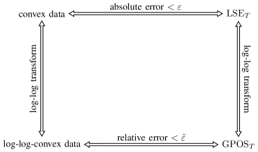
Figure 1: Relation among the classes of functions and data.

However, it is worth noticing that, since in any compact subset of $\mathbb{R}_{>0}^{n}$ bounding relative errors is equivalent to bounding absolute errors, it follows that the class $\mathrm{GPOS}_{T}$ is also such that there exists $\psi_{T}\in\mathrm{GPOS}_{T}$ such that the absolute error between $\psi_{T}(\mathbf{z}_{i})$ and $w_{i}$ can be made arbitrarily small, provided that $T\in\mathbb{R}_{>0}$ is sufficiently small.

IV Relation with feedforward neural networks

Functions in $\mathrm{LSE}_{T}$ can be modeled through a feedforward neural network ($\mathrm{FFNN}$) with one hidden layer. Indeed, consider a $\mathrm{FFNN}$ with $n$ input nodes, one hidden layer with $K$ nodes, and one output node, as depicted in Figure 2.

Figure 2: A feedforward neural network with one hidden layer.

Let the activation function of the hidden nodes be

$$s\mapsto(\exp(s/T)),$$

and let the activation of the output node be

$$s\mapsto T\log(s).$$

Each node in the hidden layer computes a term of the form $s_{k}=\langle\bm{\alpha}^{(k)},\mathbf{x}\rangle+\beta_{k}$, where the $i$-th component $\alpha^{(k)}_{i}$ of $\bm{\alpha}^{(k)}$ represents the weight between node $k$ and input $x_{i}$, and $\beta_{k}$ is the bias term of node $k$. Each node $k$ thus generates activations

$$a_{k}=\exp(\langle\bm{\alpha}^{(k)},\mathbf{x}/T\rangle+\beta_{k}/T).$$

We consider the weights from the inner nodes to the output node to be unitary, whence the output node computes $s=\sum_{k=1}^{K}a_{k}$ and then, according to the output activation function, the output layer returns the value

$$y=T\log(s)=T\log\left(\sum_{k=1}^{K}a_{k}\right).$$

We name such a network an $\mathrm{LSE\text{-}FFNN}$. Comparing the expression of $y$ with (3) it is readily seen that an $\mathrm{LSE\text{-}FFNN}$ allows us to represent any function in $\mathrm{LSE}_{T}$. We can then restate 4 as the following key theorem.

Theorem 3.

Given a collection of convex data $\mathcal{C}\doteq\{(\mathbf{x}_{i},y_{i})\}_{i=1}^{m}$ generated by an unknown convex function, for each $\varepsilon\in\mathbb{R}_{>0}$ there exists an $\mathrm{LSE\text{-}FFNN}$ such that

$$|f_{T}(\mathbf{x}_{i})-y_{i}|\leqslant\varepsilon,\quad i=1,\dots,m,$$

where $f_{T}$ is the input-output function of the $\mathrm{LSE\text{-}FFNN}$.

3 can be viewed as a specialization of the Universal Approximation Theorem [13, 14, 15, 32] to convex functions. While universal-type approximation theorems provide theoretical approximation guarantees for general FFNN on general classes of functions, our 3 only provides guarantees for data generated by convex functions. However, while general FFNN synthesize nonlinear and non-convex functions, $\mathrm{LSE\text{-}FFNN}$ are guaranteed to provide a convex input-output map, and this is a key feature of interest when the synthesized model is to be used at a later stage as a basis for optimizing over the input variables.

$\mathrm{LSE\text{-}FFNN}$s can also be used to fit log-log-convex data $\mathcal{L}=\{(\mathbf{z}_{i},w_{i})\}_{i=1}^{m}$: by applying a log-log transformation $\mathbf{x}_{i}=\log\mathbf{z}_{i}$, $y_{i}=\log w_{i}$, $i=1,\ldots,m$, we simply transform log-log-convex data into convex data $\mathcal{C}=\{(\mathbf{x}_{i},y_{i})\}_{i=1}^{m}$ and train the network on these data. Therefore, the following theorem is a direct consequence of 3 and 1.

Theorem 4.

Given a collection of log-log-convex data $\mathcal{L}\doteq\{(\mathbf{z}_{i},w_{i})\}_{i=1}^{m}$ generated by an unknown log-log-convex function, for each $\tilde{\varepsilon}\in\mathbb{R}_{>0}$ there exists an $\mathrm{LSE\text{-}FFNN}$ such that

$$\left|\frac{\exp(f_{T}(\log(\mathbf{z}_{i})))-w_{i}}{\min(\exp(f_{T}(\log(\mathbf{z}_{i}))),w_{i})}\right|\leqslant\tilde{\varepsilon},\quad i=1,\dots,m,$$

where $f_{T}$ is the input-output function of the $\mathrm{LSE\text{-}FFNN}$.

IV-A Implementation considerations

Given training data $\mathcal{C}=\{(\mathbf{x}_{i},y_{i})\}_{i=1}^{m}$, and for fixed $K$ and $T>0$, the network weights $\bm{\alpha}^{(1)},\dots,\bm{\alpha}^{(K)},\beta_{1},\ldots,\beta_{K}$ can be determined via standard training algorithms, such as the Levenberg-Marquardt algorithm [33], the gradient descent with momentum [34], or the Fletcher-Powell conjugate gradient [35], which are, for instance, efficiently implemented in Matlab through the Neural Network Toolbox [36]. These algorithms tune the network’s weights in order to minimize a loss criterion of the form

$$L=\sum_{i=1}^{m}L_{i}(f_{T}(\mathbf{x}_{i})-y_{i})+{R},$$

where the observation loss $L_{i}$ is typically a standard quadratic or an absolute value loss, and ${R}$ is a regularization term that does not depend on the training data. For given network parameters $\overrightarrow{\bm{\alpha}}$ and $\bm{\beta}$, using (4) we observe that

$$f_{T}^{(\overrightarrow{\bm{\alpha}},\bm{\beta})}(\mathbf{x}_{i})-y_{i} = Tf_{1}^{(\overrightarrow{\bm{\alpha}},\bm{\beta}/T)}(\mathbf{x}_{i}/T)-y_{i}$$

$$= T\left(f_{1}^{(\overrightarrow{\bm{\alpha}},\bm{\beta}/T)}(\mathbf{x}_{i}/T)-y_{i}/T\right).$$

Hence, the loss term $\sum_{i=1}^{m}L_{i}(f_{T}(\mathbf{x}_{i})-y_{i})$ is proportional to $\sum_{i=1}^{m}L_{i}(f_{1}(\mathbf{x}_{i}/T)-y_{i}/T)$ for the usual quadratic and absolute losses. Thus, the temperature $T>0$ can be implemented in practice by pre-scaling the data (i.e., divide the inputs and outputs by $T$), and then feeding such scaled data to an $\mathrm{LSE\text{-}FFNN}$ which synthesizes a function in the LSE (or, equivalently, $\mathrm{LSE}_{1}$) class, having activations $s\mapsto\exp(s)$ in the hidden layer and $s\mapsto\log(s)$ in the output layer.

Training and simulation of this type of $\mathrm{LSE\text{-}FFNN}$ is implemented in a package we developed, which works in conjunction with Matlab’s Neural Network Toolbox.

In numerical practice, we shall fix $T>0$ and a value of $K$, train the network with respect to the remaining model parameters as detailed above, and possibly iterate by adjusting $T$ and $K$, until a satisfactory fit is eventually found on validation data. Here, the parameter $T$ controls the smoothness of the fitting function (as $T$ increases $f_{T}$ becomes “smoother”), and the parameter $K$ controls the complexity of the model class (as $K$ increases $f_{T}$ becomes more complex).

V Applications to physical examples

We next illustrate the proposed methodology with practical numerical examples. In Section V-A we find a convex model expressing the amount of vibration transmitted by a vehicle suspension system as a function of its mechanical parameters. Similarly, in Section V-B, we derive a convex model relating the peak power generated by the chemical reaction of propane combustion as a function of the initial concentrations of all the involved chemical species.

These models are first trained using the gathered data, and next used for design (e.g., find concentrations that maximize power) by solving convex optimization and geometric programming problems via efficient numerical algorithms. This two-step process (model training followed by model exploitation for design) embodies an effective tool for performing data-driven optimization of complex physical processes.

V-A Vibration transmitted by a vehicle suspension system

In this numerical experiment, we considered the problem of identifying an $\mathrm{LSE}_{T}$ and a $\mathrm{GPOS}_{T}$ model for the amount of whole-body vibration transmitted by a vehicle suspension system having 11 degrees of freedom, as depicted in Figure 3.

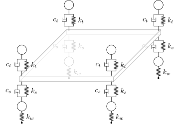
Figure 3: Model for the vehicle suspension system.

The model of the vehicle is taken from [37] and includes the dynamics of the seats, the wheels, and the suspension system. In order to measure the amount of vibration transmitted by the vehicle, it is assumed that the left wheels of the vehicle are moving on a series of two bumps with constant speed, see [37] for further details on the vehicle model.

The amount of whole-body vibration is measured following the international standard ISO-2631, [38]. Namely, the vertical acceleration of the left-set $a(t)$ is frequency-weighted through the function $H(t)$ following the directions given in Appendix A of [38], thus obtaining the filtered signal

$$a_{w}(t)=\int_{0}^{t}H(t-\tau)\,a(\tau)\,\mathrm{d}\tau.$$

Then, the amount of transmitted vibration is computed as

$$V=\left(\frac{1}{\Theta}\int_{0}^{\Theta}a_{w}^{2}(t)dt\right)^{\frac{1}{2}},$$

where $\Theta$ is the simulation time. Clearly, $V$ is a complicated function of the input parameters $k_{w}$, $k_{s}$, $k_{t}$, $c_{s}$, and $c_{t}$, that can be evaluated by simulating the dynamics given in [37]. However, manipulation and parameter design using direct and exact evaluation of $V$ by integration of the dynamics can be very costly and time consuming. Therefore, we are interested in obtaining a simpler model via an $\mathrm{LSE\text{-}FFNN}$.

It is here worth noticing that, in practice, we may not know whether the function we are dealing with is convex, log-log-convex, or neither. Nevertheless, by fitting an $\mathrm{LSE\text{-}FFNN}$ to the observed data we can obtain a convex (or log-log-convex) function approximation of the data, and check directly a posteriori if the approximation error is satisfactory or not. Further, certain types of physical data may suggest that a $\mathrm{GPOS}_{T}$ model might be suitable for modeling them: it is the case with data where the inputs are physical quantities that are inherently positive (e.g., in this case, stiffnesses and damping coefficients) and likewise the output quantity is also inherently positive (e.g., the mean-squared acceleration level).

In this example, we identified both a model in $\mathrm{LSE}_{T}$ and a model in $\mathrm{GPOS}_{T}$ for $V$. Firstly, a set of 250 data points

$$\mathcal{S}\doteq\{(\mathbf{x}_{i},V_{i})\}_{i=1}^{250},$$

has been gathered by simulating the dynamics of the system depicted in Figure 3 for randomly chosen values of $k_{w}$, $k_{s}$, $k_{t}$, $c_{s}$, and $c_{t}$ with the distributions shown in Table I.

TABLE I: Distribution of the parameters in the multi-body simulations.

Parameter	Distribution	Dimension
$k_{w}$ (stiffness of the wheel)	$\mathcal{N}(175.41,\,17.1)$	$\mathrm{kN/m}$
$k_{s}$ (stiffness of the suspension)	$\mathcal{N}(17.424,\,1.72)$	$\mathrm{kN/m}$
$k_{t}$ (stiffness of the set)	$\mathcal{N}(1.747,\,0,17)$	$\mathrm{kN/m}$
$c_{s}$ (damping of the suspension)	$\mathcal{N}(1.465,\,0.15)$	$\mathrm{kN\,s/m}$
$c_{t}$ (damping of the seat)	$\mathcal{N}(0.697,\,0.07)$	$\mathrm{kN\,s/m}$

An $\mathrm{LSE\text{-}FFNN}$ with 5 inputs and $K=10$ hidden neurons has been implemented by interfacing the Neural Network toolbox [36] with a Convex_Neural_Network module that we developed, which provides a convexnet function that can be used for training the $\mathrm{LSE\text{-}FFNN}$. The temperature parameter $T$ has been determined via a campaign of several cross validation experiments with varying values of $T$. For the $\mathrm{LSE}_{T}$, the best model in terms of mean absolute error has been obtained for $T=0.01$. The same temperature value has been obtained for the $\mathrm{GPOS}_{T}$ models.

After the training, the outputs of the $\mathrm{LSE}_{T}$ and $\mathrm{GPOS}_{T}$ models to the inputs $\{\mathbf{x}_{i}\}_{i=201}^{250}$ (which have not been used for training) have been compared with $\{V_{i}\}_{i=201}^{250}$, with the outputs of a classical $\mathrm{FFNN}$ with symmetric sigmoid activation function for the hidden layer (with the same number of hidden nodes) and linear activation function for the output layer and with the output of an $\mathrm{MA}$ function (with $10$ terms), which has been trained on the same data. In particular, the $\mathrm{MA}$ function has been trained by using the heuristic given in [8], whereas the $\mathrm{FFNN}$, the $\mathrm{LSE}_{T}$ and the $\mathrm{GPOS}_{T}$ networks have been trained by using the Neural Network Toolbox. Figure 4 and 5 depict the estimates and the approximation errors obtained by using the $\mathrm{FFNN}$, $\mathrm{MA}$, $\mathrm{LSE}_{T}$, $\mathrm{GPOS}_{T}$ models, whereas Table II summarizes the error of each model.

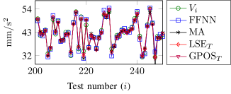
Figure 4: Results of the numerical tests.

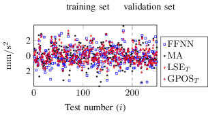
Figure 5: Absolute approximation errors.

TABLE II: Prediction errors

Method	Mean abs. err.	Mean rel. err.	Max abs. err.	Max rel. err.
$\mathrm{FFNN}$	$0.95\,\mathrm{mm/s^{2}}$	$2.36\%$	$3.54\,\mathrm{mm/s^{2}}$	$11.6\%$
$\mathrm{MA}$	$0.96\,\mathrm{mm/s^{2}}$	$2.45\%$	$5.38\,\mathrm{mm/s^{2}}$	$20.73\%$
$\mathrm{LSE}_{T}$	$0.81\,\mathrm{mm/s^{2}}$	$1.98\%$	$3.25\,\mathrm{mm/s^{2}}$	$7.85\%$
$\mathrm{GPOS}_{T}$	$0.71\,\mathrm{mm/s^{2}}$	$1.69\%$	$2.79\,\mathrm{mm/s^{2}}$	$5.87\%$

As shown by Table II, the $\mathrm{GPOS}_{T}$ model has the best performance in terms of absolute and relative errors.

The $\mathrm{FFNN}$ model $\phi$, the $\mathrm{MA}$ model $f_{0}$, the $\mathrm{LSE}_{T}$ model $f_{T}$, and the $\mathrm{GPOS}_{T}$ model $\psi_{T}$ have next been used to design the parameters $\mathbf{x}$ that minimize the amount of vibration $V$. Namely, letting $\bar{\mathbf{x}}$ be the mean value of the random variable used to find the models, the nonlinear programming problem

$$\left|\begin{array}[]{rl}\text{minimize }&\phi(\mathbf{x})\\ \text{subject to }&0.9\,\bar{\mathbf{x}}\leqslant\mathbf{x}\leqslant 1.1\,\bar{\mathbf{x}},\\ \end{array}\right.$$ (15)

has been solved by using the Matlab function fmincon. Similarly, the convex optimization problems

$$\left|\begin{array}[]{rl}\text{minimize }&f_{0}(\mathbf{x})\;\mbox{[or $f_{T}(\mathbf{x})$]}\\ \text{subject to }&0.9\,\bar{\mathbf{x}}\leqslant\mathbf{x}\leqslant 1.1\,\bar{\mathbf{x}},\\ \end{array}\right.$$ (16)

and the geometric program

$$\left|\begin{array}[]{rlll}\text{minimize }&\psi_{T}(\mathbf{x})\\ \text{subject to }&0.9\,\bar{x}_{i}\,x_{i}^{-1}\leqslant 1,&\quad i=1,\dots,5,\\ &1.1\,\bar{x}_{i}^{-1}\,x_{i}\leqslant 1,&\quad i=1,\dots,5,\\ \end{array}\right.$$ (17)

have been solved by using CVX, a package for solving convex and geometric programs [28, 39, 40, 41]. Then, the dynamics of the multibody system depicted in Figure 3 have been simulated with the optimal values gathered by solving either (15), (16), or (17). The computation of the solution to (15) required $4.813\,\mathrm{s}$ (that is larger than the computation times reported in Table III due to the fact that convex optimization tools cannot be used) and the computed optimal solution led to an amount of total vibration equal to $46.525\,\mathrm{mm/s^{2}}$. On the other hand, the results obtained by solving (16), and (17) are reported in Table III.

TABLE III: Results of the simulations with the optimal values

Problem solved	Computing time	Amount of vibration
$f_{0}$	$0.922\,\mathrm{s}$	$30.513\,\mathrm{mm/s^{2}}$
$f_{T}$	$1.628\,\mathrm{s}$	$29.723\,\mathrm{mm/s^{2}}$
$\psi_{T}$	$0.554\,\mathrm{s}$	$29.609\,\mathrm{mm/s^{2}}$

The results given in Table III highlight the effectiveness of the $\mathrm{GPOS}_{T}$ model, which indeed yields the best design in the least computing time.

V-B Combustion of propane

In this numerical experiment, we considered the problem of identifying a convex and a log-log-convex model for the peak power generated through the combustion of propane. We considered the reaction network for the combustion of propane presented in [42], which consists of 83 reactions and 29 chemical species, see Figure 6 for a graphical representation of the stoichiometric matrix of this chemical reaction network.

Figure 6: Stoichiometric matrix of the reaction network for the combustion of propane, in which each row corresponds to a different chemical reaction and each column corresponds to a different chemical species.

The instantaneous power generated by the combustion is approximatively given by

$$P(t)=\Delta_{c}H^{e}\frac{\mathrm{d}\,m(t)}{\mathrm{d}\,t},$$ (18a)

where $$\Delta_{c}H^{e} \simeq 2220\,\mathrm{kJ}/\mathrm{mol} m(t)$$ is the calorific value of the propane () and denotes the number of moles of propane. Hence, the peak power generated by this reaction is

$$\overline{P}\doteq\max_{t\in\mathbb{R}_{\geqslant 0}}P(t).$$ (18b)

Clearly, $\overline{P}$ is a function of the initial concentrations $\mathbf{x}$ of all the involved chemical species and can be obtained by performing exact numerical simulations of the chemical network (e.g., by using the stochastic simulation algorithm given in [43]), taking averages to determine the mean behavior of $m(t)$, and using (18). However, performing all these computations is rather costly, due to the fact that a large number of simulations has to be performed in order to take average. Hence, in order to maximize the effectiveness of the combustion, it is more convenient to obtain a simplified “surrogate” model relating $\mathbf{x}$ and $\overline{P}$. In particular, convex and log-log-convex models relating $\mathbf{x}$ with $\overline{P}^{-1}$ seem to be appealing since they allow the design of the initial concentrations that maximizes $\overline{P}$ by means of computationally efficient algorithms.

In this example, we identify a model in $\mathrm{LSE}_{T}$ and a model in $\mathrm{GPOS}_{T}$ for ${\overline{P}}^{-1}$ as a function of $\mathbf{x}$. We observe that, also in this example, $\mathrm{GPOS}_{T}$ models appear to be potentially well adapted to the physics of the problem, since all input variables are positive concentrations of chemicals, and the output (peak power) is also positive. First, a collection of 500 data points

$$\mathcal{S}\doteq\{(\mathbf{x}_{i},\overline{P}_{i}^{-1})\}_{i=1}^{500}$$

has been gathered by choosing randomly the initial condition $\mathbf{x}_{i}$ of the chemical reaction network with uniform distribution in the interval $[1.494,1.827]\,\mathrm{pmol/m^{3}}$, by performing $1000$ simulations of the chemical reaction network through the algorithm given in [43], by taking averages to determine the expected time behavior of $m(t)$, and using (18) to determine the value of $\overline{P}_{i}$, $i=1,\dots,500$.

Then, the function convexnet of the toolbox Convex_Neural_Network has been used to design an $\mathrm{LSE\text{-}FFNN}$ with $n=29$ input nodes, 1 output node, and 1 hidden layer with $K=3$ neurons. Several cross-validation experiments have been executed preliminarily in order to determine a satisfactory value for the temperature parameter $T$, which resulted to be $T=0.01$ for $\mathrm{LSE}_{T}$ models and $T=0.005$ for $\mathrm{GPOS}_{T}$ models.

After training the network, we considered the inputs $\{\mathbf{x}_{i}\}_{i=251}^{500}$ (which have not been used for training) and computed the corresponding outputs for the $\mathrm{LSE}_{T}$ model $f_{T}$ and of the $\mathrm{GPOS}_{T}$ model $\psi_{T}$ . These outputs are compared with $\{\overline{P}_{i}^{-1}\}_{i=251}^{500}$, with the outputs of a classical $\mathrm{FFNN}$ with symmetric sigmoid activation function for the hidden layer (with the same number of hidden nodes) and linear activation function for the output layer, which has been trained by using the same data, and with the outputs of an $\mathrm{MA}$ function $f_{0}$ (with 3 terms) that has been trained on the same data by using the heuristic given in [8]. Figure 7 and 8 depict the estimates and the approximation errors obtained by using the $\mathrm{FFNN}$, $\mathrm{MA}$, $\mathrm{LSE}_{T}$ and $\mathrm{GPOS}_{T}$ models, whereas Table IV summarizes the prediction error of each model.

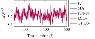
Figure 7: Results of the numerical tests.

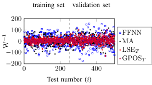
Figure 8: Approximation errors.

TABLE IV: Prediction errors

Method	Mean abs. err.	Mean rel. err.	Max abs. err.	Max rel. err.
$\mathrm{FFNN}$	$42.15\,\mathrm{W^{-1}}$	$1.28\%$	$172.75\,\mathrm{W^{-1}}$	$4.62\%$
$\mathrm{MA}$	$30.38\,\mathrm{W^{-1}}$	$9.27\%$	$115.81\,\mathrm{W^{-1}}$	$4.33\%$
$\mathrm{LSE}_{T}$	$20.48\,\mathrm{W^{-1}}$	$0.62\%$	$130.63\,\mathrm{W^{-1}}$	$4.18\%$
$\mathrm{GPOS}_{T}$	$14.94\,\mathrm{W^{-1}}$	$0.45\%$	$126.31\,\mathrm{W^{-1}}$	$4.03\%$

As shown by Table IV, the $\mathrm{LSE}_{T}$ and the $\mathrm{GPOS}_{T}$ models have improved prediction capabilities with respect to the classical $\mathrm{FFNN}$ and the $\mathrm{MA}$ model. In particular, the model in $\mathrm{GPOS}_{T}$ presents the best approximation performance. Moreover, the model $f_{0}$ in $\mathrm{MA}$ , the model $f_{T}$ in $\mathrm{LSE}_{T}$ and the model $\psi_{T}$ in $\mathrm{GPOS}_{T}$, can be used to efficiently design the initial concentrations $\mathbf{x}$ that are within the considered range and that maximize the peak power. In fact, the convex optimization problems

$$\left|\begin{array}[]{rl}\text{minimize }&f_{0}(\mathbf{x})\;\mbox{[or $f_{T}(\mathbf{x})$]}\\ \text{subject to }&1.49\cdot 10^{-12}\leqslant\mathbf{x}\leqslant 1.83\cdot 10^{-12},\end{array}\right.$$ (19)

as well as the geometric program

$$\left|\begin{array}[]{rll}\text{minimize }&\psi_{T}(\mathbf{x})\\ \text{subject to }&1.49\cdot 10^{-12}\,x_{i}^{-1}\geqslant 1,&i=1,\dots,29,\\ &1.83\cdot 10^{-12}\,x_{i}\geqslant 1,&i=1,\dots,29,\\ \end{array}\right.$$ (20)

can be efficiently solved by using any solver able to deal with convex optimization problems. On the other hand, letting $\phi$ be the $\mathrm{FFNN}$ model, solving a problem of the form (19) with $\phi$ as the objective may be rather challenging due to the fact that it need not be (and generically is not) convex. In fact, by attempting at solving such nonlinear programming problem via fmincon we failed, whereas we have been able to find the solutions of problems (19) and (20) by using the Matlab toolbox CVX. Table V reports the computing time required to determine such solutions and the corresponding peak power obtained by simulating the chemical reaction network.

TABLE V: Results of the simulations with the optimal values

Problem solved	Computing time	Peak power
$f_{0}$	$1.279\mathrm{s}$	$0.363\,\mathrm{mW}$
$f_{t}$	$2.968\mathrm{s}$	$0.368\,\mathrm{mW}$
$\psi_{T}$	$0.655\,\mathrm{s}$	$0.369\,\mathrm{mW}$

As shown by Table V, the model in $\mathrm{GPOS}_{T}$ presents the best performance in the considered example.

VI Conclusions

A feedforward neural network with exponential activation functions in the inner layer and logarithmic activation in the output layer can approximate with arbitrary precision any convex function on a convex and compact input domain. Similarly, any log-log-convex function can be approximated to arbitrary relative precision by a class of generalized posynomial functions. This allows us to construct convex (or log-log-convex) models that approximate observed data, with the advantage over standard feedforward networks that the synthesised input-output map is convex (or log-log-convex) in the input variables, which makes it readily amenable to efficient optimization via convex or geometric programming.

The techniques given in this paper enable data-driven optimization-based design methods that apply convex optimization on a surrogate model obtained from data. Of course, some data might be more suitable than other to be approximated via convex or log-log-convex models: if the (unknown) data generating function underlying the observed data is indeed convex (or log-log-convex), then we may expect very good results in the fitting via LSE_T functions (or $\mathrm{GPOS}_{T}$ functions). Actually, even when convexity or log-log-convexity of the data generating function is not known a priori, we can find in many cases a data fit that is of quality comparable, or even better, than the one obtained via general non-convex neural network models, with the clear advantage of having a model possessing the additional and desirable feature of convexity.

Giuseppe C. Calafiore (S ’14, F ’18) received the “Laurea” degree in Electrical Engineering from Politecnico di Torino in 1993, and the Ph.D. degree in Information and System Theory from Politecnico di Torino, in 1997. He is with the faculty of Dipartimento di Electronics and Telecommunications, Politecnico di Torino, where he currently serves as a full professor and coordinator of the Systems and Data Science lab. Dr. Calafiore held several visiting positions at international institutions: at the Information Systems Laboratory (ISL), Stanford University, California, in 1995; at the Ecole Nationale Supérieure de Techniques Avanceés (ENSTA), Paris, in 1998; and at the University of California at Berkeley, in 1999, 2003 and 2007. He had an appointment as a Senior Fellow at the Institute of Pure and Applied Mathematics (IPAM), University of California at Los Angeles, in 2010. He had appointments as a Visiting Professor at EECS UC Berkeley in 2017 and at the Haas Business School in 2018. He is a Fellow of the Italian National Research Council (CNR). He has been an Associate Editor for the IEEE Transactions on Systems, Man, and Cybernetics (T-SMC), for the IEEE Transactions on Automation Science and Engineering (T-ASE), and for Journal Européen des Systémes Automatisés (JESA). He currently serves as an Associate Editor for the IEEE Transactions on Automatic Control. Dr. Calafiore is the author of more than 180 journal and conference proceedings papers, and of eight books. He is a fellow member of the IEEE since 2018. He received the IEEE Control System Society “George S. Axelby” Outstanding Paper Award in 2008. His research interests are in the fields of convex optimization, randomized algorithms, machine learning, computational finance, and identification and control of uncertain systems.

Stephane Gaubert graduated from École Polytechnique, Palaiseau, in 1988. He got a PhD degree in Mathematics and Automatic Control from École Nationale Supérieure des Mines de Paris in 1992. He is senior research scientist (Directeur de Recherche) at INRIA Saclay – Île-de-France and member of CMAP (Centre de Mathématiques Appliquées, École Polytechnique, CNRS), head of a joint research team, teaching at École Polytechnique. He coordinates the Gaspard Monge corporate sponsorship Program for Optimization and Operations Research (PGMO), of Fondation Mathématique Hadamard. His interests include tropical geometry, optimization, game theory, monotone or nonexpansive dynamical systems, and applications of mathematics to decision making and to the verification of programs or systems.

Corrado Possieri received his bachelor’s and master’s degrees in Medical engineering and his Ph.D. degree in Computer Science, Control and Geoinformation from the University of Roma Tor Vergata, Italy, in 2011, 2013, and 2016, respectively. From September 2015 to June 2016, he visited the University of California, Santa Barbara (UCSB). Currently, he is Assistant Professor at the Politecnico di Torino. He is a member of the IFAC TC on Control Design. His research interests include stability and control of hybrid systems, the application of computational algebraic geometry techniques to control problems, stochastic systems, and optimization.

References

- [1] R. Yondoa, E. Andrés, and E. Valeroa, “A review on design of experiments and surrogate models in aircraft real-time and many-query aerodynamic analyses,” Progress in Aerospace Sciences, vol. 96, pp. 23–61, 2018.
- [2] A. Forrester, A. Sobester, and A. Keane, Engineering design via surrogate modelling: a practical guide. John Wiley & Sons, 2008.
- [3] D. Gorissen, I. Couckuyt, P. Demeester, T. Dhaene, and K. Crombecq, “A surrogate modeling and adaptive sampling toolbox for computer based design,” Journal of Machine Learning Research, vol. 11, no. Jul, pp. 2051–2055, 2010.
- [4] G. C. Calafiore and L. El Ghaoui, Optimization models. Cambridge Univ. Press, 2014.
- [5] S. Boyd and L. Vandenberghe, Convex optimization. Cambridge University Press, 2004.
- [6] F. A. Potra and S. J. Wright, “Interior-point methods,” J. Comput. Appl. Math., vol. 124, no. 1-2, pp. 281–302, 2000.
- [7] R. T. Rockafellar, “Lagrange multipliers and optimality,” SIAM Review, vol. 35, no. 2, pp. 183–238, 1993.
- [8] A. Magnani and S. P. Boyd, “Convex piecewise-linear fitting,” Optim. Eng., vol. 10, no. 1, pp. 1–17, 2009.
- [9] J. Kim, L. Vandenberghe, and C.-K. K. Yang, “Convex piecewise-linear modeling method for circuit optimization via geometric programming,” IEEE Trans. Comput. Aided Des. Integr. Circuits Syst., vol. 29, no. 11, pp. 1823–1827, 2010.
- [10] W. Hoburg, P. Kirschen, and P. Abbeel, “Data fitting with geometric-programming-compatible softmax functions,” Optim. Eng., vol. 17, no. 4, pp. 897–918, 2016.
- [11] W. Daems, G. Gielen, and W. Sansen, “Simulation-based generation of posynomial performance models for the sizing of analog integrated circuits,” IEEE Trans. Comput. Aided Des. Integr. Circuits Syst., vol. 22, no. 5, pp. 517–534, 2003.
- [12] G. C. Calafiore, L. M. El Ghaoui, and C. Novara, “Sparse identification of posynomial models,” Automatica, vol. 59, pp. 27–34, 2015.
- [13] G. Cybenko, “Approximation by superpositions of a sigmoidal function,” Math. Control Signals Syst., vol. 2, no. 4, pp. 303–314, 1989.
- [14] H. White, “Connectionist nonparametric regression: Multilayer feedforward networks can learn arbitrary mappings,” Neural networks, vol. 3, no. 5, pp. 535–549, 1990.
- [15] K. Hornik, “Approximation capabilities of multilayer feedforward networks,” Neural Networks, vol. 4, no. 2, pp. 251 – 257, 1991.
- [16] D. W. Ruck, S. K. Rogers, M. Kabrisky, M. E. Oxley, and B. W. Suter, “The multilayer perceptron as an approximation to a Bayes optimal discriminant function,” IEEE Trans. Neural Networks, vol. 1, no. 4, pp. 296–298, 1990.
- [17] V. T. S. Elanayar and Y. C. Shin, “Radial basis function neural network for approximation and estimation of nonlinear stochastic dynamic systems,” IEEE Trans. Neural Networks, vol. 5, no. 4, pp. 594–603, 1994.
- [18] P. Andras, “Function approximation using combined unsupervised and supervised learning,” IEEE Trans. Neural Networks Learn. Syst., vol. 25, no. 3, pp. 495–505, 2014.
- [19] V. Charisopoulos and P. Maragos, “Morphological perceptrons: Geometry and training algorithms,” in Mathematical Morphology and Its Applications to Signal and Image Processing (J. Angulo, S. Velasco-Forero, and F. Meyer, eds.), pp. 3–15, Springer Int. Publishing, 2017.
- [20] L. Zhang, G. Naitzat, and L.-H. Lim, “Tropical geometry of deep neural networks,” in Proceedings of the 35th International Conference on Machine Learning, Stockholm, Sweden, PMLR 80, 2018, 2018. To appear.
- [21] J. Borwein and A. S. Lewis, Convex analysis and nonlinear optimization: theory and examples. Springer, 2010.
- [22] B. Klartag and E. Milman, “Centroid bodies and the logarithmic Laplace transform–a unified approach,” J. Funct. Anal., vol. 262, no. 1, pp. 10–34, 2012.
- [23] S. Brazitikos, A. Giannopoulos, P. Valettas, and B.-H. Vritsiou, Geometry of Isotropic Convex Bodies. AMS, 2014.
- [24] O. Viro, “Dequantization of real algebraic geometry on logarithmic paper,” in European Congress of Mathematics, Vol. I (Barcelona, 2000), vol. 201 of Progr. Math., pp. 135–146, Birkhäuser, Basel, 2001.
- [25] I. Itenberg, G. Mikhalkin, and E. Shustin, Tropical algebraic geometry. Oberwolfach seminars, Birkhäuser, 2007.
- [26] G. L. Litvinov, “Maslov dequantization, idempotent and tropical mathematics: A brief introduction,” Journal of Mathematical Sciences, vol. 140, no. 3, pp. 426–444, 2007.
- [27] J. Kingman, “A convexity property of positive matrices,” Quart. J. Math. Oxford, vol. 12, pp. 283–284, 1961.
- [28] S. Boyd, S.-J. Kim, L. Vandenberghe, and A. Hassibi, “A tutorial on geometric programming,” Optim. Eng., vol. 8, no. 1, pp. 67–127, 2007.
- [29] R. T. Rockafellar, Convex Analysis. Princeton Univ. Press, 1970.
- [30] L. Schwartz, Topologie générale et analyse fonctionnelle. Hermann, 1993.
- [31] C. L. a. Jean-Baptiste Hiriart-Urruty, Convex Analysis and Minimization Algorithms II: Advanced Theory and Bundle Methods. Grundlehren der mathematischen Wissenschaften 306, Springer-Verlag Berlin Heidelberg, 1 ed., 1993.
- [32] K. Hornik, M. Stinchcombe, and H. White, “Multilayer feedforward networks are universal approximators,” Neural networks, vol. 2, no. 5, pp. 359–366, 1989.
- [33] D. W. Marquardt, “An algorithm for least-squares estimation of nonlinear parameters,” J. Soc. Ind. Appl. Math., vol. 11, no. 2, pp. 431–441, 1963.
- [34] I. Sutskever, J. Martens, G. Dahl, and G. Hinton, “On the importance of initialization and momentum in deep learning,” in Int. Conf. Mach. Learn., pp. 1139–1147, 2013.
- [35] L. Scales, Introduction to non-linear optimization. Springer, 1985.
- [36] M. H. Beale, M. T. Hagan, and H. B. Demuth, “Neural Network Toolbox User’s Guide,” 2018. The MathWorks Inc.
- [37] S. H. Zareh, A. Sarrafan, A. A. A. Khayyat, and A. Zabihollah, “Intelligent semi-active vibration control of eleven degrees of freedom suspension system using magnetorheological dampers,” J. Mech. Sci. Technol., vol. 26, no. 2, pp. 323–334, 2012.
- [38] International Organization for Standardization, “Mechanical Vibration and shock – Evaluation of human exposure to whole-body vibration,” Standard ISO 2631-1:1997(E), May 1997.
- [39] M. Grant and S. Boyd, “CVX: Matlab software for disciplined convex programming, version 2.1.” http://cvxr.com/cvx, Mar. 2014.
- [40] M. Grant and S. Boyd, “Graph implementations for nonsmooth convex programs,” in Recent Advances in Learning and Control (V. Blondel, S. Boyd, and H. Kimura, eds.), Lecture Notes in Control and Information Sciences, pp. 95–110, Springer-Verlag Limited, 2008.
- [41] R. J. Duffin, E. L. Peterson, and C. M. Zener, Geometric programming: theory and application. J. Wiley & Sons, 1967.
- [42] C. J. Jachimowski, “Chemical kinetic reaction mechanism for the combustion of propane,” Combustion and Flame, vol. 55, no. 2, pp. 213–224, 1984.
- [43] C. Possieri and A. R. Teel, “Stochastic robust simulation and stability properties of chemical reaction networks,” IEEE Trans. Control Network Syst., 2018.