Rethinking Machine Learning Development and Deployment for Edge Devices

Abstract

Machine learning (ML), especially deep learning is made possible by the availability of big data, enormous compute power and, often overlooked, development tools or frameworks. As the algorithms become mature and efficient, more and more ML inference is moving out of datacenters/cloud and deployed on edge devices. This model deployment process can be challenging as the deployment environment and requirements can be substantially different from those during model development. In this paper, we propose a new ML development and deployment approach that is specially designed and optimized for inference-only deployment on edge devices. We build a prototype and demonstrate that this approach can address all the deployment challenges and result in more efficient and high-quality solutions.

1 Introduction

Deep neural networks (DNNs) have demonstrated near-human accuracy in a wide range of applications, including image classification, speech recognition and natural language processing. The availability of large training datasets and compute power has been key enablers for this breakthrough. Arguably and often overlooked, the availability of ML development tools or frameworks, such as Caffe [1] and TensorFlow [2], is also important as they allow more developers to easily experiment with new networks/algorithms and quickly evaluate them for new types of applications.

There are a lot of benefits in running neural network inference locally at the edge [3, 4]. A lot of research efforts have been focusing on designing more efficient networks [5, 6, 7], more compact numerical representation [8, 9, 10, 11, 12] and more powerful inference engines both in terms of dedicated hardware [13, 14] and optimized software [15, 16]. Together, these make it possible to run DNN-based solutions on edge and even deeply embedded devices [17].

Despite the good progress on demonstrating the capabilities of running DNNs at the edge, the NN model deployment process remains as both a challenging and tedious process. In most scenarios, the deployment targets can be embedded devices with limited memory and compute resources. Running the NN inference inside a full-blown framework environment may be impractical and unnecessary. Most existing solutions implement either an inference-only runtime [18] or a static compilation flow [19]. But there can still be some challenges when using these solutions to deploy a pre-trained and pre-optimized NN model from ML frameworks. These challenges are mostly created by the difference between framework environment and inference environment, which includes:

• Operator availability: ML frameworks are usually designed to be flexible and can include many experimental or customized operators. This enables ML developers to experiment with new types of network architecture, but at the same time makes it difficult to deploy these models with inference-only implementation, which is typically optimized for efficiency.

• Operator behavior: Inference-only implementations, especially hardware implementations can be novel in their approaches, e.g., the use of Winograd convolution [20], different numerical representation [9, 21], data compression [22] or even non-digital computation [23, 24]. The operators in these implementations are likely to be different from the standard 32-bit floating point (fp32) based implementations inside most ML frameworks.

In this work, we explore an alternative approach of ML development and deployment targeting deployment at the edge. We build a prototype targeting Arm Cortex-M CPUs with CMSIS-NN [15] and demonstrate that this approach can greatly simplify the model deployment process and generate solutions with better efficiency and quality.

2 Current Approach

Current ML development and deployment approach is shown in Figure 1. Application developers use the ML frameworks to construct their NN models, perform training and evaluate the accuracy. Based on the evaluation results, they can go back and refine or optimize their models. After this development stage, a trained model is generated by the framework. The deployment tool, typically offered by the deployment platform vendor, takes this trained model as the input and constructs a deployable solution that runs on the target platform.

This deployment process can be divided into two parts. The first part is the model execution, which includes parsing the NN model graph, mapping the operators to the available implementation, and then re-constructing the execution graph with proper resource allocation. The second part is the parameter conversion which takes the trained weights or parameters and converts them into the format and values that can be fed into their operator implementation while retaining or closely replicating the expected behavior.

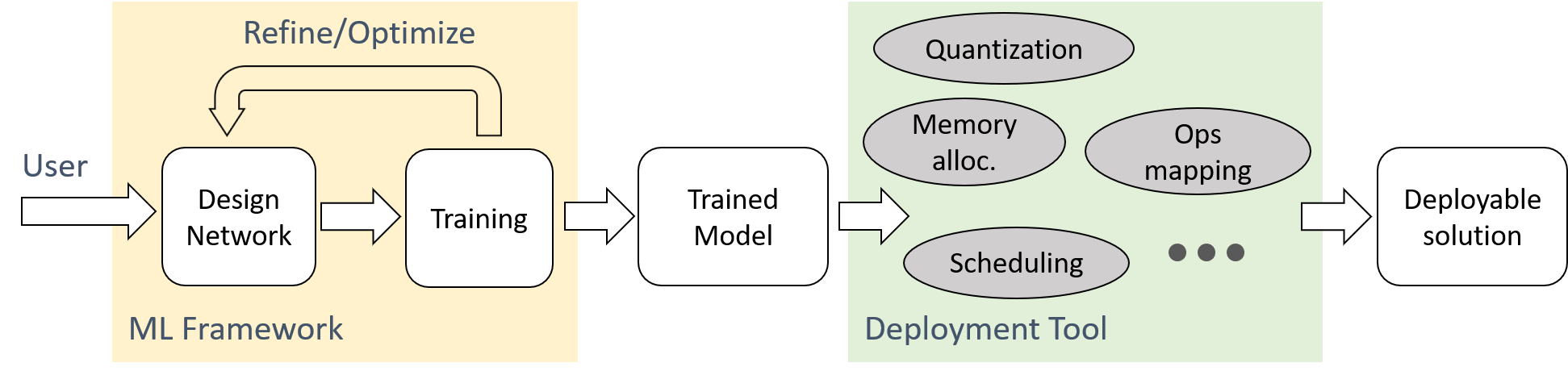
Figure 1: Current ML development and deployment approach. The shaded blocks are vendor-specific parts.

The difference in operator availability and behavior, as discussed earlier, poses challenges to these two parts of the deployment process. Standard formats [25] or APIs [26] can be a solution to the operator availability issue. This solution, however, also forces the inference implementation to be generic (e.g., to support all of the standard operators) or with enough flexibility rather than being able to optimize for specialization. Since the ML algorithms and frameworks may evolve over time, these standards can also be a moving target, which makes it difficult for the implementation, especially the hardware implementation, to be future-proof. The operator behavior issue is another limiting factor that restricts the implementation design space. The implemented operators have to closely replicate the operators that are in the ML frameworks, which may not be the most implementation friendly and efficient options.

Conceptually, there are three ML models during the entire ML development and deployment process: the model that is designed and optimized by the developer, the model that is trained in ML framework and the model that is deployed on the device. The design optimization of these three models using current approach can be represented by the following equation:

$$\operatorname*{arg\,max}(model)=\operatorname*{arg\,max}(train)\approx\operatorname*{arg\,max}(deploy)$$ (1)

$\operatorname*{arg\,max}(model)$ represents the process of model optimization during ML development. In the current approach, where the user specifies and constructs the NN model inside the framework using native operators, this model is the same as the model that gets trained by the framework. Therefore, all the model optimization is equivalent to optimizing the model that is trained in ML framework. This is represented by the first half of the equation, i.e., $\operatorname*{arg\,max}(model)=\operatorname*{arg\,max}(train)$. However, as discussed earlier, the deployed model generated by the deployment tools may not be exactly the same as the trained model. As a result, the model optimization during the development process ($\operatorname*{arg\,max}(model)$) is only an approximation of optimizing the deployed model ($\operatorname*{arg\,max}(deploy)$). This is represented by the second half of the equation.

The other problem for this approach is the deployment uncertainty. The accuracy of the deployed model is unknown at model development time, which makes it difficult for the developer to control and guarantee solution quality. This accuracy uncertainty, a.k.a. accuracy loss, may be quantified empirically with some benchmark models. But it is still difficult to guarantee whether this can be generalized to all kinds of models.

3 Proposed Approach

If the target is deployment on the edge devices, the deployment quality (i.e., $\operatorname*{arg\,max}(deploy)$) should be the primary optimization target, rather than the model specified and trained in the ML framework (i.e., $\operatorname*{arg\,max}(train)$).

To achieve this, we proposed the ML development and deployment approach shown in Fig. 2. Unlike current approach, the users, which are the solution developers, will specify their network models using the deployment tool with an operator library from the deployment platform vendor. The deployment tool will generate a deployable but untrained solution, i.e., a model that can run on their platform, but without the trained parameters. As part of the deployment tool, the vendor should also be responsible to create an operator model library that can represent their operators and be used to create a trainable model inside the ML framework. This trainable model should have a forward inference path that behaves exactly the same as the implemented operators, and a backward path for the ML framework to perform training in order to generate the appropriate weights and parameters. In this approach, the validation results from the ML framework will be the same as the deployment results, so that the user can use these results to refine or further optimize their network models.

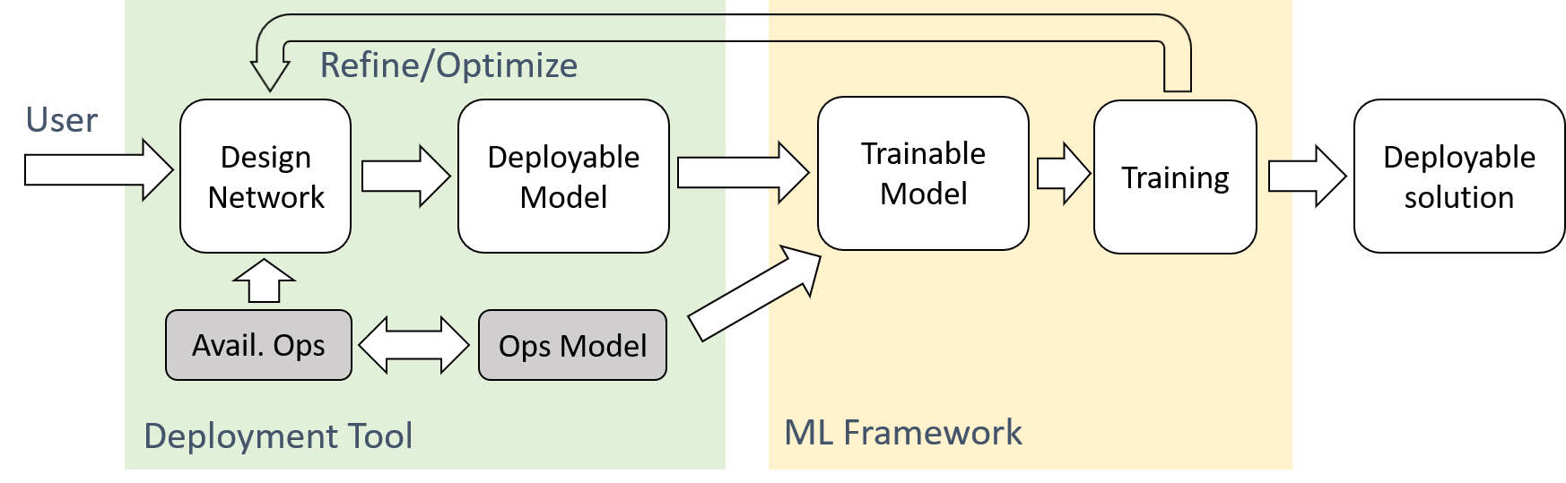
Figure 2: Proposed ML development and deployment approach. The shaded blocks are vendor-specific parts.

This proposed approach can be represented as the following equation:

$$\operatorname*{arg\,max}(model)=\operatorname*{arg\,max}(deploy)\approx\operatorname*{arg\,max}(train)$$ (2)

where the model constructed by the user is the same as the model that is going to be deployed on the device, i.e., $\operatorname*{arg\,max}(model)=\operatorname*{arg\,max}(deploy)$. In this approach, the training target is the trainable model generated by the deployment tool rather than the constructed or deployed model. Therefore, all the training optimization is only an approximation of optimizing the actual model, which is represented by the second half of the equation.

This approach addresses the operator availability issue by moving the network specification process into the deployment environment. This can also give accurate estimates of the inference latency, memory footprints and energy cost, which helps network designer to pick the more efficient operators for the targeting platform [27].

The operator behavior issue in this approach becomes the requirements to make sure that the implemented operators have trainable representations inside the ML framework. This is a relatively easier problem than making sure that the implemented operators behave similarly to the equivalent ones in the ML framework, as the solutions for the latter problem is a subset of the former one.

The other potential advantage of this approach is that the trainable model inside the ML framework can also be used as the golden model for debug and validation purposes. This avoids the need to implement an execution model of the deployment platform from scratch. Re-using the trainable model can also leverage all the already well-optimized computation routines/kernels inside the framework.

4 Proof-of-Concept Experiments

4.1 Operator Model Implementation

To validate the proposed approach, we implement a prototype of an operator library and an operator model library targeting Arm Cortex-M CPUs with CMSIS-NN [15] and TensorFlow [2]. In this work, we refer this prototype as KANJI.

The computation kernels in CMSIS-NN implements int8 fixed-point computation. Therefore, the quantization is performed symmetrically around zero. The quantization step is forced to be power-of-2 so that the transformation between different quantization formats becomes simple bit-level shifting. To replicate the same quantization setup as that in CMSIS-NN, we design a specific quantization block as shown in Fig. 3. Inspired by how batch normalization is implemented, this quantization block keeps track of the data distribution of the input and sets the quantization range accordingly. The value quantization is performed by using the $FakeQuant$ operator from TensorFlow.

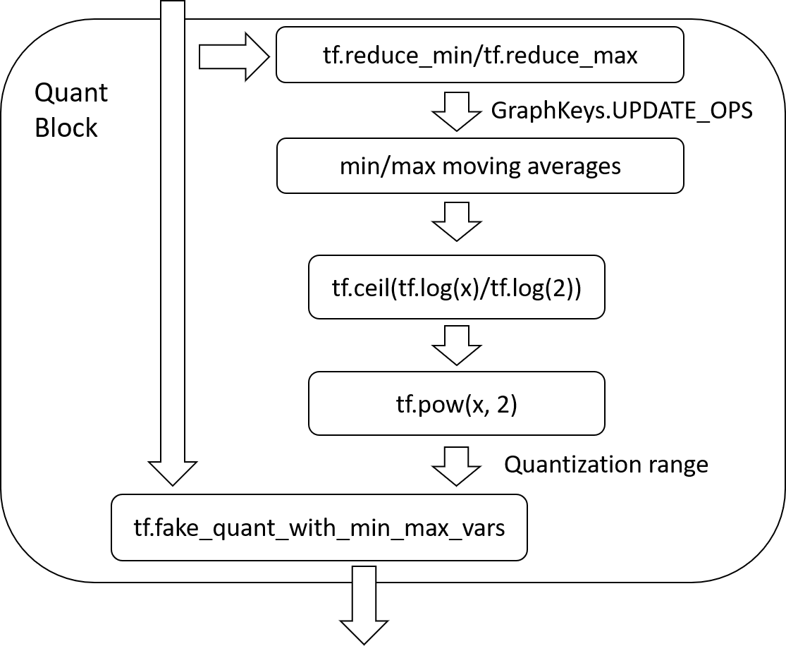
Figure 3: Convolution Model Implementation using TensorFlow operators for CMSIS-NN

The operator library includes image pre-processing, convolution layer, fully-connected layer, max pooling and ReLU. Some of the layers, e.g., max pooling and ReLU, have the same behaviors in TensorFlow and CMSIS-NN, so the default TensorFlow operators are used. For other layers, we implement the computation using the quantization block and built-in TensorFlow operators.

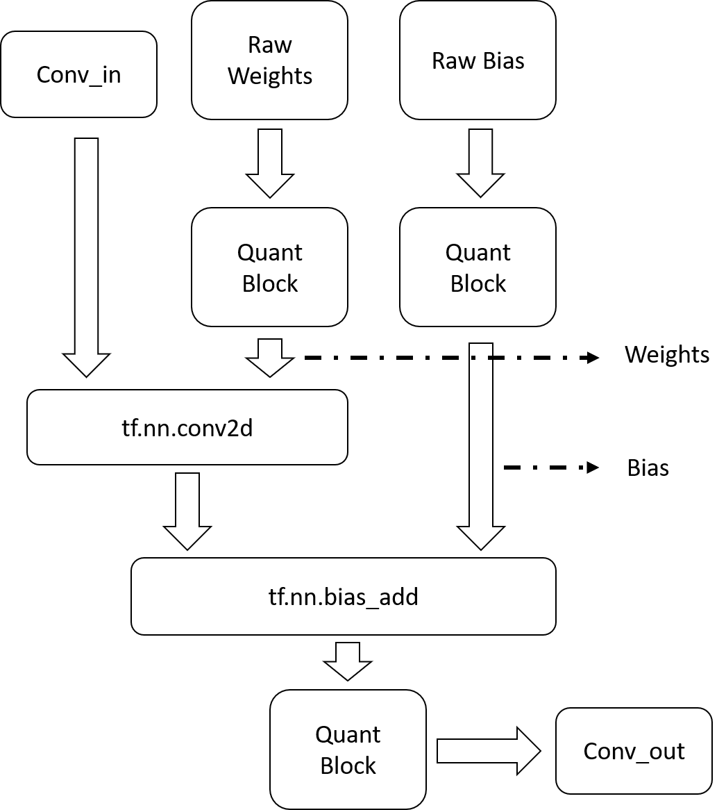
Figure 4: Convolution Model Implementation using TensorFlow Operators for CMSIS-NN

An example of the convolution operator implementation is shown in Fig. 4. In this convolution model, both raw weights and bias are fp32 trainable parameters. The quantization block is tracking the moving average of the data min/max and adjust the quantization range accordingly. The int8 weights and bias values used by CMSIS-NN convolution function will be the tensor value after the quantization block. The quantization ranges for inputs, weights, bias and outputs are used to determine the $out\_shift$ and $bias\_shift$ parameters for the convolution functions in CMSIS-NN. We also validate that the operator behavior in TensorFlow is identical to the behavior of the CMSIS-NN kernel running on Cortex-M CPUs.

4.2 Experimental Results

In this section, we will evaluate the implemented prototype KANJI. In particular, we want to evaluate the impacts of the following:

• $\operatorname*{arg\,max}(model)\approx\operatorname*{arg\,max}(train)$ vs. $\operatorname*{arg\,max}(model)=\operatorname*{arg\,max}(train)$: comparing the capabilities (i.e., accuracy) of the same NN model trained with different approaches. This is described in Section 4.2.1.

• $\operatorname*{arg\,max}(model)=\operatorname*{arg\,max}(deploy)$ vs. $\operatorname*{arg\,max}(model)\approx\operatorname*{arg\,max}(deploy)$: studying the potential improvements on inference efficiency and quality using KANJI. This is described in Section 4.2.2.

4.2.1 Accuracy Impacts

To evaluate the accuracy, we implement the CNN example described in CMSIS-NN [15] using both default fp32 based training and KANJI. The CNN example is designed for CIFAR-10 dataset and has 3 convolution layers, 3 pooling layers and 1 fully-connected layer. The numbers of output channels for the three convolution layers are 32, 32 and 64, respectively. The data augmentation, learning rate control and optimizer setup is the same as the CIFAR-10 example in TensorFlow.

The accuracy results are summarized in Table 1. We also repeat the experiments with different network sizes by changing the number of output channels in the convolution layers. In most cases, the results are similar between the fp32 model and the KANJI int8 model. We observe a trend that KANJI performs relatively better on smaller network sizes than larger ones. But this may be an artifact of the training setup optimizer and learning rate setup, which will be discussed in Section 5.1.

Table 1: Accuracy results for CIFAR-10 Dataset with different network sizes.

Number of Conv Channels	fp32	int8 KANJI
(16, 16, 32)	77.3%	78.5%
(32, 32, 64)	80.8%	81.9%
(48, 48, 96)	83.1%	83.0%
(64, 64, 128)	84.2%	83.7%

We also carry out the experiments with larger networks and datasets. We use VGG network architecture and perform the training for both CIFAR-100 and tiny-imagenet datasets. The accuracy results are summarized in Table 2. Similar to CIFAR-10 results, the accuracy results are very similar for int8 KANJI models and fp32 models.

Table 2: Accuracy results with VGG for CIFAR-100 and tiny-imagenet dataset.

Data set	fp32	int8 KANJI
CIFAR-100 top1	59.5%	59.6%
CIFAR-100 top3	77.9%	77.4%
tiny-imagenet top1	42.0%	42.0%
tiny-imagenet top3	60.0%	60.1%

4.2.2 Input-dependent vs. Input-independent Operators

One important advantage of the proposed approach is that it allow users to use the operators that can be implemented more efficiently, rather than the default operators in the ML frameworks. In this section, we show through examples that our proposed approach can generate more efficient inference solutions with similar or better accuracy.

An example is the use of input-independent operators instead of the input-dependent ones. For example, it is known that normalizing the input data can improve the effectiveness of the training and the model accuracy. One of the most popular image pre-processing operators in TensorFlow is $per\_image\_standardization$ where each image channel is shifted and scaled to have zero mean and unit variance. This is an input-dependent operator as the amount of shifting and scaling depends on the input data distribution. These values can vary for different input images and have to be calculated for each inference run. Caffe extracts the mean value for each pixel by scanning the entire training set and storing them in the $mean.binaryproto$ file and included as part of the model parameters. At inference time, these mean values are subtracted from the input image. This image pre-processing operator is input independent as the same mean pixel value is subtracted regardless of what the input image is. In KANJI, we implement an operator that is similar to $batch\_norm$ but without offset (i.e., $\beta$) and scale (i.e., $\gamma$), so the data normalization process is input-independent and the storage overhead is kept minimal. We also force the shifted mean (i.e., $\mu$) to be integer, and scaling (i.e., $\sigma$) to be power-of-2, so that the process becomes simple integer subtraction and shifting. The details of different image pre-processing options are listed in Table 3

Table 3: Different image pre-processing operators.

Image Pre-Processing Operator	Input Dependence	Memory Overhead	Runtime Overhead
$per\_image\_standardization$	Yes	Low	High
$mean.binaryproto$	No	High	Low
$batch\_norm$-like	No	Low	Low

The other example is asymmetric quantization vs. symmetric quantization. Quantization, in this context, refers to the process of mapping a floating-point value to an integer value. The relationship between the floating-point value ($value\_fp$) and quantized integer value ($value\_int$) can be represented with the quantization range ($[min\_fp,max\_fp)$) and quantization step ($step\_fp$) by the following equation:

$$value\_fp=min\_fp+(value\_int-min\_int)*step\_fp$$ (3)

There are different ways to perform quantization. The simplest way is symmetric quantization with power-of-2 step value, i.e., $min\_fp+max\_fp=0$ and $step\_fp=2^{n}$ where n is a integer value. This is also referred as fixed-point quantization and is used by CMSIS-NN. The other popular way is asymmetric quantization, e.g., supported by Android NNAPI [26] where quantization range and step size can be arbitrary value.

The symmetry of the quantization scheme affects the quantized computation. For example, quantized matrix multiplication can be implemented as regular integer matrix multiplication if the quantization is symmetric. If the quantization is asymmetric, implementation similar to GEMMLOWP [28] can be used, where the bulk part of the computation is still regular integer matrix multiplication, and additional routines are needed to compute the impacts of non-zero offsets. To quantify the overhead of these additional routines, we also implement GEMMLOWP-like matrix multiplication routine for asymmetric quantization. Experiments on Cortex-M CPUs show that the runtime overhead is about 15% for typical network sizes.

The other important part is how to quantize the computation outputs (i.e., accumulators). One way to quantize the outputs is to find out the min and max values and apply the quantization accordingly. This is an input-dependent process and usually requires to store all raw outputs temporarily. This can result in 2-4X increase in runtime memory footprint. On the contrary, CMSIS-NN forces the quantization step to be power-of-2 so that the output quantization can be done on-the-fly with simple shifting.

These implementation friendly operators can improve the inference efficiency. They can also affect the model accuracy. We repeat the CIFAR-10 experiments with different image pre-processing techniques and quantization schemes. The accuracy results are shown in Table 4. Among the three image pre-processing operators, the $batch\_norm$-like operator gives the best accuracy. The quantization does not seem to degrade the accuracy. In the case of KANJI, where quantization is accounted for during training, the accuracy may even be higher than the fp32 counterpart.

Table 4: Network accuracy on CIFAR-10 with different image pre-processing and quantization.

Input Pre-Processing	Quantization	Accuracy
$per\_image\_standardization$	None (fp32)	81.2%
$per\_image\_standardization$	8-bit asymmetric	81.2%
$mean.binaryproto$	None (fp32)	81.5%
$mean.binaryproto$	8-bit, symmetric	81.5%
$batch\_norm$-like	None (fp32)	81.8%
$batch\_norm$-like	KANJI	81.9%

5 Discussion

5.1 Model Training

The training process using the proposed approach can be different from training a native fp32 model. This difference can include the effectiveness of different training setups, such as loss functions, optimizers, batch sizes, and learning rates. For example, the training loss curves of native fp32 training and KANJI using different optimizers and initial learning rates are plotted in Fig. 5. For SGD optimizer, loss reduces faster but saturates earlier for fp32 training (SGD_fp32), comparing to KANJI (SGD_KANJI), even though they have the same initial learning rate of $0.1$. Since the training target in KANJI is an 8-bit model, there may be some damping effects in gradient approximation and updates, making the effective learning rate smaller. We repeat the experiments for KANJI with an increased initial learning rate of $0.15$ (SGD_KANJI_p15). In this case, the loss saturates to a similar level as SGD_fp32. This difference in learning rate is not observed with ADAM optimizer, with the loss curves for both fp32 training (ADAM_fp32) and KANJI (ADAM_KANJI) following similar trends.

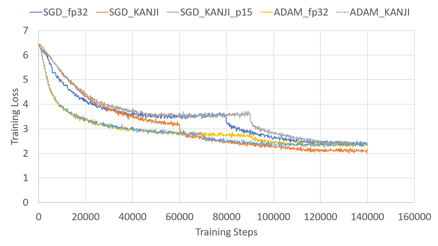
Figure 5: Training loss for tiny-imagenet with different optimizer and initial learning rate.

The configuration and hyperparameter setting during the training can have big impact on the final model accuracy. In our experiments, we try to keep the same setup for KANJI and native fp32 training to get fair comparisons. Comparing to the training process using the proposed approach, the training process of native fp32 model is relatively better understood and optimized. More learning and research of the training process could further improve the solution quality of the proposed approach.

The other noticeable difference is the training time. Training using the proposed approach is likely to be slower. Based on our experiments, training time per step in KANJI is about 20% to 25% slower than training the fp32 model. But the total training time comparison may be different and will also depend on how the model converges. If the training efficiency is critical, a hybrid approach can also be used where the model is pre-trained in fp32 and fine-tuned using the proposed approach.

5.2 Pre-trained Models

Although the proposed approach shown in Fig. 2 assumes that the entire process is starting from scratch, in many scenarios, it is both necessary and beneficial to be able to incorporate a pre-trained model into the development and deployment process. The hybrid training approach discussed in previous section is one example.

There are also many well-trained and well-optimized NN models that can be directly used or re-targeted (e.g., through transfer learning). Being able to use these pre-trained models can help avoid the dependence on the complete training dataset and save the training cost.

Our proposed approach can also be used to deploy a pre-trained model. The deployment flow is shown in Fig. 6. The flow is similar to current approach (shown in Fig. 1) where (a). operators in the trained model have to be mapped into the implemented ones, and (b). trained weights/parameters are converted into the formats that match the operator implementation. But the quality requirements (i.e., accuracy loss) of these conversions can be relaxed as it offers re-training capabilities that may recover the accuracy loss.

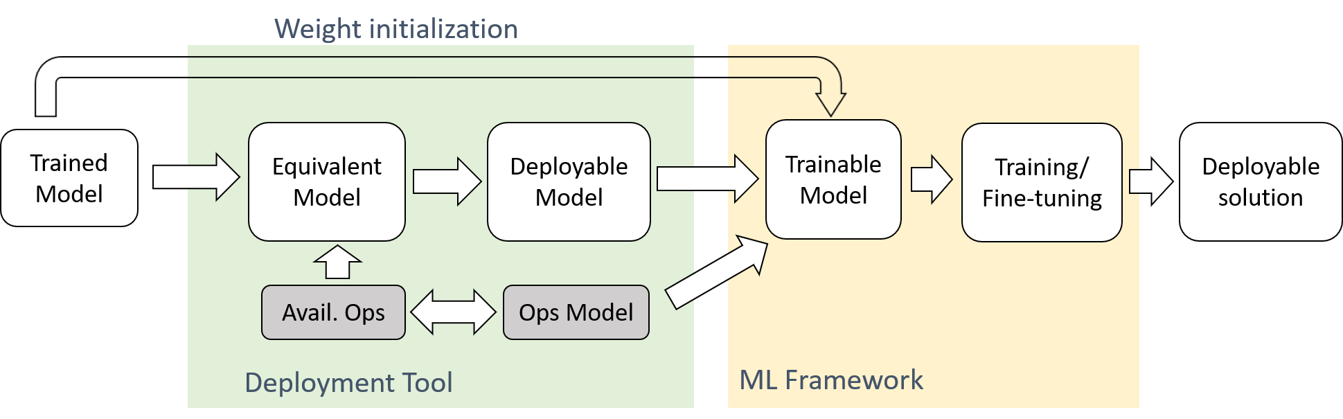
Figure 6: Pre-trained model deployment using proposed approach.

6 Conclusion

Big data and ample compute power have been widely considered as the two key enablers for deep learning. Though typically overlooked, the availability of proper tooling, such as the ML frameworks, is also important to enable more developers to experiment new ideas more easily and productively.

As more and more ML development and deployment targets edge devices, there is the question that whether current ML development and deployment approach offers enough flexibility allowed in the implementation and guarantee quality during the deployment. In this work, we propose a new ML development and deployment approach to address these issues. We build a prototype KANJI for Arm Cortex-M CPUs with CMSIS-NN and demonstrate that this proposed approach can remove all the deployment challenges and generate solutions that are more efficient and with better quality.

References

- [1] Yangqing Jia, Evan Shelhamer, Jeff Donahue, Sergey Karayev, Jonathan Long, Ross Girshick, Sergio Guadarrama, and Trevor Darrell. Caffe: Convolutional architecture for fast feature embedding. arXiv preprint arXiv:1408.5093, 2014.
- [2] Martín Abadi, Ashish Agarwal, Paul Barham, Eugene Brevdo, Zhifeng Chen, Craig Citro, Greg S Corrado, Andy Davis, Jeffrey Dean, Matthieu Devin, et al. Tensorflow: Large-scale machine learning on heterogeneous distributed systems. arXiv preprint arXiv:1603.04467, 2016.
- [3] https://community.arm.com/processors/b/blog/posts/machine-learning-moving-to-the-network-edge-to-improve-next-generation-services.
- [4] https://petewarden.com/2018/06/11/why-the-future-of-machine-learning-is-tiny/.
- [5] Forrest N Iandola, Song Han, Matthew W Moskewicz, Khalid Ashraf, William J Dally, and Kurt Keutzer. Squeezenet: Alexnet-level accuracy with 50x fewer parameters and< 0.5 mb model size. arXiv preprint arXiv:1602.07360, 2016.
- [6] Andrew G Howard, Menglong Zhu, Bo Chen, Dmitry Kalenichenko, Weijun Wang, Tobias Weyand, Marco Andreetto, and Hartwig Adam. Mobilenets: Efficient convolutional neural networks for mobile vision applications. arXiv preprint arXiv:1704.04861, 2017.
- [7] Gao Huang, Zhuang Liu, Kilian Q Weinberger, and Laurens van der Maaten. Densely connected convolutional networks. In Proceedings of the IEEE conference on computer vision and pattern recognition, volume 1, page 3, 2017.
- [8] Darryl Lin, Sachin Talathi, and Sreekanth Annapureddy. Fixed point quantization of deep convolutional networks. In International Conference on Machine Learning, pages 2849–2858, 2016.
- [9] Eric Chung, Jeremy Fowers, Kalin Ovtcharov, Michael Papamichael, Adrian Caulfield, Todd Massengil, Ming Liu, Daniel Lo, Shlomi Alkalay, Michael Haselman, et al. Accelerating persistent neural networks at datacenter scale. HotChips, 2017.
- [10] Liangzhen Lai, Naveen Suda, and Vikas Chandra. Deep convolutional neural network inference with floating-point weights and fixed-point activations. arXiv preprint arXiv:1703.03073, 2017.
- [11] Sean O Settle, Manasa Bollavaram, Paolo D’Alberto, Elliott Delaye, Oscar Fernandez, Nicholas Fraser, Aaron Ng, Ashish Sirasao, and Michael Wu. Quantizing convolutional neural networks for low-power high-throughput inference engines. arXiv preprint arXiv:1805.07941, 2018.
- [12] Matthieu Courbariaux and Yoshua Bengio. Binarynet: Training deep neural networks with weights and activations constrained to +1 or -1. arXiv:1602.02830, 2016.
- [13] Norman P Jouppi, Cliff Young, Nishant Patil, David Patterson, Gaurav Agrawal, Raminder Bajwa, Sarah Bates, Suresh Bhatia, Nan Boden, Al Borchers, et al. In-datacenter performance analysis of a tensor processing unit. In Proceedings of the 44th Annual International Symposium on Computer Architecture, pages 1–12. ACM, 2017.
- [14] Yu-Hsin Chen, Tushar Krishna, Joel S Emer, and Vivienne Sze. Eyeriss: An energy-efficient reconfigurable accelerator for deep convolutional neural networks. IEEE Journal of Solid-State Circuits, 2016.
- [15] Liangzhen Lai, Naveen Suda, and Vikas Chandra. Cmsis-nn: Efficient neural network kernels for arm cortex-m cpus. arXiv preprint arXiv:1801.06601, 2018.
- [16] Sharan Chetlur, Cliff Woolley, Philippe Vandermersch, Jonathan Cohen, John Tran, Bryan Catanzaro, and Evan Shelhamer. cudnn: Efficient primitives for deep learning. arXiv preprint arXiv:1410.0759, 2014.
- [17] Yundong Zhang, Naveen Suda, Liangzhen Lai, and Vikas Chandra. Hello edge: Keyword spotting on microcontrollers. arXiv preprint arXiv:1711.07128, 2017.
- [18] https://github.com/tensorflow/tensorflow/tree/master/tensorflow/contrib/lite.
- [19] https://github.com/tensorflow/tensorflow/tree/master/tensorflow/compiler/xla.
- [20] Andrew Lavin and Scott Gray. Fast algorithms for convolutional neural networks. In Proceedings of the IEEE Conference on Computer Vision and Pattern Recognition, pages 4013–4021, 2016.
- [21] Hardik Sharma, Jongse Park, Naveen Suda, Liangzhen Lai, Benson Chau, Joon Kyung Kim, Vikas Chandra, and Hadi Esmaeilzadeh. Bit fusion: Bit-level dynamically composable architecture for accelerating deep neural networks. arXiv preprint arXiv:1712.01507, 2017.
- [22] Song Han, Huizi Mao, and William J Dally. Deep compression: Compressing deep neural networks with pruning, trained quantization and huffman coding. arXiv preprint arXiv:1510.00149, 2015.
- [23] Ali Shafiee, Anirban Nag, Naveen Muralimanohar, Rajeev Balasubramonian, John Paul Strachan, Miao Hu, R Stanley Williams, and Vivek Srikumar. Isaac: A convolutional neural network accelerator with in-situ analog arithmetic in crossbars. ACM SIGARCH Computer Architecture News, 44(3):14–26, 2016.
- [24] Filipp Akopyan, Jun Sawada, Andrew Cassidy, Rodrigo Alvarez-Icaza, John Arthur, Paul Merolla, Nabil Imam, Yutaka Nakamura, Pallab Datta, Gi-Joon Nam, et al. Truenorth: Design and tool flow of a 65 mw 1 million neuron programmable neurosynaptic chip. IEEE Transactions on Computer-Aided Design of Integrated Circuits and Systems, 34(10):1537–1557, 2015.
- [25] https://github.com/onnx.
- [26] https://developer.android.com/ndk/guides/neuralnetworks/.
- [27] Liangzhen Lai, Naveen Suda, and Vikas Chandra. Not all ops are created equal! arXiv preprint arXiv:1801.04326, 2018.
- [28] https://github.com/google/gemmlowp.