Minimax functions on Galton-Watson trees

Abstract.

We consider the behaviour of minimax recursions defined on random trees. Such recursions give the value of a general class of two-player combinatorial games. We examine in particular the case where the tree is given by a Galton-Watson branching process, truncated at some depth $2n$, and the terminal values of the level-$2n$ nodes are drawn independently from some common distribution. The case of a regular tree was previously considered by Pearl, who showed that as $n\to\infty$ the value of the game converges to a constant, and by Ali Khan, Devroye and Neininger, who obtained a distributional limit under a suitable rescaling.

For a general offspring distribution, there is a surprisingly rich variety of behaviour: the (unrescaled) value of the game may converge to a constant, or to a discrete limit with several atoms, or to a continuous distribution. We also give distributional limits under suitable rescalings in various cases.

We also address questions of endogeny. Suppose the game is played on a tree with many levels, so that the terminal values are far from the root. To be confident of playing a good first move, do we need to see the whole tree and its terminal values, or can we play close to optimally by inspecting just the first few levels of the tree? The answers again depend in an interesting way on the offspring distribution.

We also mention several open questions.

1. Introduction

In this paper we consider the behaviour of minimax recursions defined on random trees.

Consider a finite rooted tree with depth $m$. We will call the root “level 0”, the children of the root “level 1”, and so on. Suppose every node at levels $0,1,\dots,m-1$ has at least one child; the nodes at level $m$ are all leaves. Suppose every leaf node (i.e. every node at level $m$) has some real value associated to it. Then recursively propagate the values towards the root in a minimax way: each node at an odd level gets a value which is the max of the values of its children, and each node at an even level gets a value which is the min of the values of its children.

This minimax procedure has a natural interpretation in terms of a two player game. Two players alternate turns; a token starts at the root, and a move of the game consists of moving the token from its current node to one of the children of that node. The leaf nodes are terminal positions; the outome of the game is the value associated to the leaf node where the game ends. Player 1 is trying to minimise this outcome, and player 2 is trying to maximise it. The outcome of the game with “optimal play” is the value associated to the root.

Suppose the terminal values are random, drawn independently from some common distribution.

Pearl [10] considered the case where the tree is regular (every non-leaf node has $d$ children for some $d\geq 2$) and the terminal values are independent and uniformly distributed on the interval $[0,1]$. For simplicity assume that the depth of the tree is even; write $W_{2n}$ for a random variable representing the value at the root of a tree of depth $2n$. Pearl showed that $W_{2n}$ converges in distribution to a constant as $n\to\infty$. This result was refined by Ali Khan, Devroye and Neininger [2], who derived an asymptotic distribution for $W_{2n}$ after appropriate rescaling.

In this paper we consider the case where the tree is given by a Galton-Watson branching process, truncated at level $2n$. This generalisation leads to a surpsingly rich variety of behaviour, depending on the offspring distribution of the branching process. For example, the limiting distribution of $W_{2n}$ may be concentrated at a single point (as in the regular case), or may now have several atoms, or may even be continuous.

There is also a rich interplay between the two sources of randomness now present in the model (the tree itself, and the terminal values at the leaves). Suppose we play the game on a tree with many levels, so that the terminal values are far from the root. In order to be confident of playing a good first move, do we need to see the whole tree and terminal values, or can we play close to optimally by inspecting just the structure of the first few levels of the tree? Such questions can be formulated precisely in terms of the endogeny property for certain recursive tree processes, as introduced by [1]. The answers again depend in an interesting way on the offspring distribution.

Such questions concerning the relative importance of local tree structure and terminal values are of considerable interest in understanding the effectiveness of certain tree-search algorithms such as Monte Carlo tree search (MCTS) – see [6] for a survey. MCTS has famously been applied in recent years to games such as go, where it provided a considerable increase in playing strength [7] even before being allied with powerful deep learning techniques [12]. For some games, simple versions of these algorithms, without local evaluation functions, and with only very crude input from the terminal values (given for example by “random rollouts” through unexplored parts of the tree), are nonetheless able to converge quickly towards good lines of play. Understanding which aspects of a game’s structure make such convergence possible is an interesting challenge both in theoretical and in practical terms.

Our main resuts concerning distributional limits are presented in the next section. In Section 2 we discuss a range of examples and mention some open problems. The results about endogeny are given in Section 3. The main proofs are given in Section 4 and Section 5.

Before that we mention some recent related work. Broutin, Devroye and Fraiman [4] consider recursive distributional equations (including those of minimax type) defined on Galton-Watson trees conditioned to have a given total size $n$. Holroyd and Martin [8] consider minimax-type games (and various misère and asymmetric variants) defined on (perhaps infinite) Galton-Watson trees, with particular emphasis on the nature of phase transitions for the outcomes of the game as the underlying offspring distribution varies (see Section 2 for further comments). Note that in both [4] and [8], unlike in the case of this paper, the offspring distribution puts positive weight at $0$, so that there are leaves close to the root.

Similar questions arise in the context of random AND/OR trees and random Boolean functions. For example the model of Pemantle and Ward [11] involves a regular tree in which each node independently is a max or a min with equal probability; see Section 2.2 for comments on the relation to a particular case of our model. See for example Broutin and Mailler [5] for a variety of recent results in a more general setting, and many relevant references.

1.1. Main results

Consider a Galton-Watson tree with an offspring distribution with mass function $p_{1},p_{2},p_{3},\dots$ on $\{1,2,3,\dots\}$ (note that every individual has at least one child). Let $G(x)=\sum_{k=0}^{\infty}p_{k}x^{k}$ be the probability generating function of the offspring distribution (which is a strictly increasing function mapping $[0,1]$ to $[0,1]$ bijectively). We will also write throughout

(1.1) $$R(x)=1-G(x)$$

and

(1.2) $$f(x)=R(R(x)).$$

Truncate the tree at level $2n$, so that all the vertices at level $2n$ are leaves. Let the terminal values associated to the leaves be i.i.d. uniform on $[0,1]$ (independently of the structure of the tree). Recursively, assign values to the internal nodes of the tree (in particular, to the root) using the minimax procedure defined above. See Figure 1.1 for an illustration.

Figure 1.1. An example of a minimax tree, with $4$ levels. Here all non-leaf nodes have 1, 2 or 3 children.

(Note that there is a nothing particularly special about uniform boundary conditions. By a simple rescaling we can map between this case and the case of i.i.d. boundary values from any other continuous distribution. Later we will also consider discrete boundary values, for example those taking values only 0 and 1, where we can interpret 0 as a win for the first player, and 1 as a win for the second player).

We denote by $W_{2n}$ the random variable associated with the root of a tree of depth $2n$. The we have a distributional recursion:

(1.3) $$W_{2n}\stackrel{{\scriptstyle d}}{{=}}\min_{1\leq i\leq M}\max_{1\leq j\leq M_{i}}W^{(i,j)}_{2n-2},$$

where $M$ and $M_{1},M_{2},M_{3},\dots$ are i.i.d. draws from the offspring distribution, and $W^{(i,j)}_{2n-2}$, $i,j\in{\mathbb{N}}$, are i.i.d. copies of the random variable $W_{2n-2}$, independent of $M$ and $\{M_{i}\}$.

Then a simple generating function computation (see the beginning of Section 4) gives

(1.4) $${\mathbb{P}}\left(W_{2n}\leq x\right)=f\big{(}{\mathbb{P}}(W_{2n-2}\leq x)\big{)},$$

where $f$ is defined at (1.2). So to look at the behaviour of the $W_{2n}$ for large $n$, we will be interested in the function $f$ and in particular its fixed points.

We begin with the results for the case of a regular tree.

Theorem 1.1.

Suppose $p_{d}=1$ for some $d\geq 2$.

• (Pearl [10])

  $$W_{2n}\stackrel{{\scriptstyle d}}{{\to}}w\text{ as }n\to\infty,$$

  where $q$ is the unique fixed point in $(0,1)$ of the function $f_{d\operatorname{-reg}}$ defined by

  (1.5) $$f_{d\operatorname{-reg}}(x)=1-\left(1-x^{d}\right)^{d}.$$

• (Ali Khan, Devroye and Neininger[2]) Let $\xi=f_{d\operatorname{-reg}}^{\prime}(q)$. Then

  $$\xi^{n}\left(W_{2n}-q\right)\stackrel{{\scriptstyle d}}{{\to}}W\text{ as }n\to\infty,$$

  where $W$ has a continuous distribution function $F_{W}$ which satisfies $F_{W}(x)=f_{d\operatorname{-reg}}(F_{W}(x/\xi))$.

Now we will consider general offspring distributions. Since $G$ is increasing and bijective as a function from $[0,1]$ to $[0,1]$, we have that $R=1-G$ is decreasing and bijective. and $f=R\circ R$ is again increasing and bijective. Also $G$ is analytic on $[0,1)$, so that $f$ is analytic on $(0,1)$.

We’ll be particularly interested in fixed points of the function $f$. The function $R$ itself has a single fixed point, which is obviously also a fixed point of $f$. Otherwise the fixed points of $f$ come in pairs: if $q$ is one then so is $R(q)$. One such pair are the points 0 and 1. We will say that a fixed point $q$ of $f$ is unstable from the right if $q<1$ and $\displaystyle\lim_{\epsilon\to 0}\lim_{n\to\infty}f^{n}(q+\epsilon)>q$; similarly unstable from the left if $q>0$ and $\displaystyle\lim_{\epsilon\to 0}\lim_{n\to\infty}f^{n}(q-\epsilon)<q$.

For a regular tree, Theorem 1.1 tells us that the distribution of $W_{2n}$ converges to a constant. For general distributions, we still have convergence in distribution, but now we may have a “genuinely random outcome” in the limit as the tree becomes large; the limiting distribution may have more than one atom (and in some surprising cases, the distribution of $W_{2n}$ can simply be the same uniform distribution for all $n$).

Theorem 1.2.

$W_{2n}\stackrel{{\scriptstyle d}}{{\to}}W$ as $n\to\infty$, for some random variable $W$. There are two cases.

• If $f$ is the identity function, then $W_{2n}\sim U[0,1]$ for all $n$.

• Otherwise, let $Q$ be the set of fixed points of $f$ which are unstable from at least one side.

  Then $W$ is discrete and has atoms precisely at the elements of $Q$.

  For $q\in Q$, define

  $$q_{-}{} =\begin{cases}\sup\{x:x<q,x=f(x)\},&\textrm{if $q>0$ and $q$ is unstable from the left}\\ q&\textrm{otherwise}\end{cases}$$

  (1.6) $$q_{+}{} =\begin{cases}\inf\{x:x>q,x=f(x)\},&\textrm{if $q<1$ and $q$ is unstable from the right}\\ q&\textrm{otherwise}\end{cases}.$$

  Then ${\mathbb{P}}(W=q)=q_{+}-q_{-}$.

It’s not hard to show that $x\in Q$ if and only if $R(x)\in Q$. Hence again the atoms of the distributional limit $W$ come in pairs, with the possible exception of the fixed point of $R$. In Section 2.1, we comment in particular on the case where $W$ has atoms at $0$ and $1$.

For $q\in(0,1)$, we may write (1.6) alternatively as $q_{-}=\displaystyle\lim_{\epsilon\to 0}\lim_{n\to\infty}f^{n}(q-\epsilon)$ and $q_{+}=\displaystyle\lim_{\epsilon\to 0}\lim_{n\to\infty}f^{n}(q+\epsilon)$ (this follows straightforwardly from the monotonicity and continuity of $f$).

In the next results we consider fluctuations around the atoms of the limiting distributions obtained in Theorem 1.2(b). The appropriate rescaling around a point $q\in Q$ depends on the derivative of $\xi=f^{\prime}(q)$. If $q\in Q$ then we must have $\xi\geq 1$.

Theorem 1.3.

Consider the model defined by (1.3). Assume that $f$ is not the identity function and let $Q$ be the set of fixed points of $f$ unstable from at least one side.

Let $q\in Q$. Define $q_{-}$ and $q_{+}$ as at (1.6), and let $\xi=f^{\prime}(q)$. Then:

1. If $1<\xi<\infty$, then

   $$\mathcal{L}\left(\xi^{n}(W_{2n}-q)\ |\ W_{2n}\in[q_{-},q_{+}]\right)\xrightarrow[]{}\mathcal{L}(V)\textrm{ as }n\rightarrow\infty,$$

   where $V$ is a random variable with a continuous distribution function.

2. Suppose $\xi=1$, and $k\geq 2$ is such that $f^{(r)}(q)=0$ for $1<r<k$ and $f^{(k)}(q)\neq 0$. Then

   $$\mathcal{L}\left(n^{\frac{1}{k-1}}(W_{2n}-q)\ |\ W_{2n}\in[q_{-},q_{+}]\right)\xrightarrow{}\mathcal{L}(V),$$

   where for $a=\left(\frac{k(k-2)!}{f^{(k)}(q)}\right)^{\frac{1}{k-1}}$ we have $V=\begin{cases}a&\textrm{w.p. }\frac{q_{+}-q}{q_{+}-q_{-}}\\ -a&\textrm{w.p. }\frac{q-q_{-}}{q_{+}-q_{-}}\end{cases}$.

3. If $\xi=\infty$, then $q\in\{0,1\}$. Assume now that

   (1.7) $$\mathbb{E}(M\mathbb{I}_{M\leq n})=\sum_{k=1}^{n}kp_{k}\sim cn^{\rho}\text{ as }n\to\infty$$

   for some $c>0$ and $\rho\in(0,1)$, where $M$ is distributed according to the offspring distribution of the Galton-Watson tree, and let $K=\min\{i:p_{i}\neq 0\}$. Then $K<1/(1-\rho)$, and $|f(t)-q|\sim C|t-q|^{K(1-\rho)}$ as $t\to q$ for some $C>0$. Moreover,

   $$\mathcal{L}(-[K(1-\rho)]^{n}\log|W_{2n}-q|\ |\ W_{2n}\in[q_{-},q_{+}])\xrightarrow[]{}\mathcal{L}(Y),$$

   where $Y$ is a random variable such that ${\mathbb{P}}(Y\in(0,\infty))=1$.

The scaling limits in part (a) are the closest ones to the result for the regular tree from Theorem 1.1. Note that when $q$ is an endpoint of the interval, the limiting distribution $V$ is now one-sided, supported on $(0,\infty)$ when $q=0$ and on $(-\infty,0)$ when $q=1$.

For part (b), recall that $f$ is analytic on $(0,1)$ so certainly if $q\in(0,1)$, such a $k$ exists. Conceivably, there might be no such $k$ in some cases where $q=0$ or $q=1$ (although we know of no example where analyticity fails at $0$ or $1$ except when the derivative is infinite).

On the other hand, many cases with $\xi=\infty$ are not covered by part (c). It seems challenging to describe all possible asymptotics; however, the assumption (1.7) is satisfied for an important class of power-law distributions with infinite mean, satisfying ${\mathbb{P}}(X>x)\sim x^{1-\alpha}$ with $\alpha\in(1,2)$.

2. Examples, discussion and open questions

Our final main results, concerning the endogeny property, will be stated in Section 3. Before that, we discuss a variety of examples illustrating the results of Theorems 1.2 and 1.3.

First consider a case where each node has $1$ or $3$ children. This simple family already displays an interesting range of behaviours. Let $p_{1}=p$ and $p_{3}=1-p$, for $p\in[0,1]$. In Figure 2.1, we plot the function $f(x)-x$ for $x\in[0,1]$, for a variety of values of $p$. Fixed points of $f$ correspond to zeros of the curve. A crossing from negative to positive corresponds to an unstable fixed point.

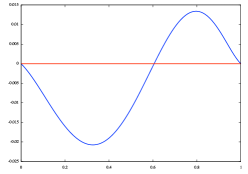
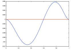
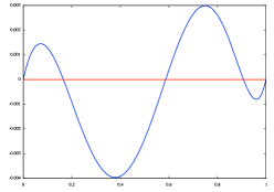
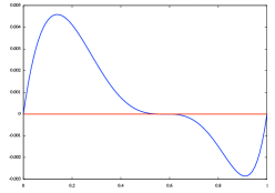
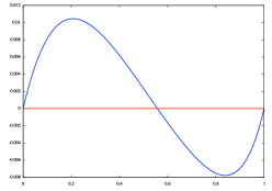
Figure 2.1. The function $f(x)-x$ for $x\in[0,1]$ for the family of distributions with $p_{1}=p$ and $p_{3}=1-p$, with (a) $p=0.45$, (b) $p=0.5$, (c) $p=0.55$, (d) $p=0.598$, and (e) $p=0.7$.

When $p<0.5$, the points 0 and 1 are stable and there is a unique unstable fixed point in $(0,1)$, just as in the case of a regular tree; $W_{2n}$ converges to a constant. At $p=0.5$, we have $f^{\prime}(0)=f^{\prime}(1)=1$; the slope of $f^{\prime}(x)-x$ at 0 and 1 is 0, but the points are still stable. For $p>0.5$, the points 0 and 1 are unstable, and the limiting distribution $W$ in Theorem 1.2 puts positive mass at 0 and 1. At first, there is also positive mass at another fixed point in $(0,1)$. However above a critical point at roughly $p=0.598$, two of the fixed points disappear, leaving only a stable fixed point in $(0,1)$, and the limiting distribution is concentrated only on the points 0 and 1.

Some further illustrative examples are shown in Figure 2.2.

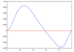
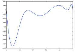
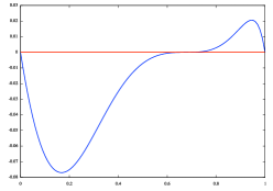
Figure 2.2. The function $f(x)-x$ for $x\in[0,1]$ in three further cases: (a) $p_{1}=0.5$, $p_{2}=0.25$, $p_{4}=0.25$; (b) $p_{2}=0.783$, $p_{30}=0.217$, and (c) $p_{2}=0.705$ and $p_{12}=0.295$.

For these distributions (the second and third are only approximate), we see points $q\in Q$ with $f^{\prime}(q)=1$, and so the rescalings of Theorem 1.3(b), which are polynomial rather than exponential, apply. In Figure 2.2(a) the relevant fixed points are at $0$ and $1$, and in Figure 2.2(a), they appear as “touchpoints” in the graph of $f(x)-x$ and so are unstable from one side only; in these cases only one of the points $a$ and $-a$ in Theorem 1.3(b) receives positive mass. By contrast, in Figure 2.2(c), the point of inflection gives a fixed point which is unstable on both sides.

In passing, we mention briefly another interesting aspect of some of the above examples, concerning phase transitions. As we vary the offspring distribution, we see points where, for example, the number of atoms of the limiting distribution $W$ changes. Often, the transition can be continuous: as the offspring distribution is varied, an existing atom may split into several new atoms (as may happen when a point of inflection occurs as in Figure 2.1(d) or Figure 2.2(c)), or new atoms may appear whose weight grows continously from $0$ (such as happens at the points $0$ and $1$ in Figure 2.1(b)). On the other hand, we can also see discontinuous transitions in cases such as Figure 2.2(b); one can perturb the offspring distribution in an arbitrarily small way to remove the “touchpoints” seen there, so that the atoms of $W$ inside $(0,1)$ disappear and all there mass jumps to the endpoints $0$ and $1$. Such ideas, expressed only vaguely here, are studied in a closely related context in [8].

2.1. Atoms at endpoints

The limiting distribution $W$ in Theorem 1.2 may have atoms at 0 and 1. We note the following simple criterion:

Proposition 2.1.

Let $\mu$ be the mean of the offspring distribution.

• If $p_{1}\mu<1$ then ${\mathbb{P}}(W=0)={\mathbb{P}}(W=1)=0$.

• If $p_{1}\mu>1$ (including the case $p_{1}>0$ and $\mu=\infty$) then ${\mathbb{P}}(W=0)>0$ and ${\mathbb{P}}(W=1)>0$.

If $p_{1}\mu=1$, or if $p_{1}=0$ and $\mu=\infty$, either case is possible. The proof of the result is straightforward. Since $f=R\circ R$ we have $f^{\prime}(x)=R^{\prime}(R(x))R^{\prime}(x)$. Then since $R(0)=1$ and $R(1)=0$, and since $R^{\prime}=-G^{\prime}$, we have $f^{\prime}(0)=f^{\prime}(1)=G^{\prime}(0)G^{\prime}(1)=\mu p_{1}$ (assuming $\mu<\infty$); and we know that a fixed point $q$ of $f$ is an atom of $W$ if $f^{\prime}(q)>1$, and not if $f^{\prime}(q)<1$.

There is a rather direct interpretation of the condition $p_{1}\mu>1$ in terms of the Galton-Watson tree and the play of the game. Consider the set of paths in the tree, starting at the root, with the following property: every vertex along the path at an odd level has only one child. The union of these paths gives a subtree containing the root. For a vertex at an even level (such as the root), the expected number of grandchildren in the subtree is $p_{1}\mu$, since the vertex itself has an average of $\mu$ children, and each of those has precisely one child with probability $p_{1}$. Considering only even levels, this then gives a branching process with mean offspring $p_{1}\mu$; if $p_{1}\mu>1$, then this branching process is supercritical and survives for ever with positive probability. In that case, by keeping the game within this tree, the first player can ensure that the second player never has any choice at all; all the second player’s moves are forced. For the game truncated at level $2n$, the first player can choose between all the nodes at level $2n$ which are within the subtree; from this it can be shown that ${\mathbb{P}}(W=0)$ is at least as big as the probability that this branching process survives.

2.2. The case $f(x)\equiv x$, and related open questions

Suppose the offspring distribution is such that $f$ is the identity function. Then from (1.4), if we put independent values at the leaves from any given distribution, then the value at the root has that same distribution (hence the statement in Theorem 1.2(a)). Perhaps surprisingly, this property is not restricted to the trivial case where $p_{1}=1$.

Here are some families of examples where $f=R\circ R=(1-G)\circ(1-G)$ is the identity (i.e. $R$ is an involution):

• Any geometric distribution. If $p_{k}=p(1-p)^{k-1}$ for $p\in(0,1)$, then $G(x)=\frac{p}{1-(1-p)x}$ and so $R(x)=\frac{1-x}{1-(1-p)x}$, and one can check $f(x)=x$.

• Let $G(x)=\left[1-(1-x)^{1/n}\right]^{n}$, for $n=1,2,3,\dots$. Via a binomial expansion, one can express $G$ has a power series expansion with non-negative coefficients, and $G(1)=1$, so $G$ is indeed a probability generating function. The coefficient of $x^{k}$ is non-zero for $k\geq n$.

• Let $G(x)=1-\left(1-x^{n}\right)^{1/n}$, for $n=1,2,3,\dots$. Again $G$ has a power series expansion with non-negative coefficients summing to 1. The coefficient of $x^{k}$ is non-zero when $k$ is a multiple of $n$.

These are far from the only cases. For a general source of examples, consider function $S(x,y)$ from $[0,1]^{2}$ to $[0,1]$ which is symmetric, increasing in each coordinate, and has $S(1,0)=S(0,1)=0$. If we define a function $R$ by setting $S(x,y)=0$ and writing $y=R(x)$, then $R$ is indeed an involution. Some such functions $R$ have power series expansions, and in some of those cases $G=1-R$ has all coefficients positive, as needed for a probability generating function. For example, $S(x,y)=y^{2}+y+x^{2}+x-2=0$ gives $R(x)=[\sqrt{9-4x-4x^{2}}-1]/2$, in which case one can obtain straightforwardly that $G=1-R$ is a generating function.

We note several questions that it might be interesting to understand further:

• Can one describe in some nice way the class of all distributions for which $f$ is the identity? For the class of examples described in the previous paragraph, can one describe nicely which functions $S(x,y)$ lead to functions $R$ which have power series expansions, and then which of those yield a generating function $G$?

• Are the geometric distributions in example (a) above the only such distributions with finite mean? More generally, what types of tail decay are possible? For (a), the tail $\sum_{r=k}^{\infty}p_{r}$ of course decays exponentially in $k$, while for (b) and (c) it decays as $k^{-1/n}$.

• Are there direct probabilistic arguments explaining the fact that $f$ becomes the identity in these cases, in terms of the underlying process on the tree?

  One case where it’s possible to make such an argument is the $n=2$ case in (b) above. Here $p_{k}$ is the probability that the cluster containing the origin has size $k$ for critical percolation on the binary tree (these coefficients are closely related to the Catalan numbers). Having made this identification, one can connect the minimax recursion on our random tree to an analogous recursion in the model studied by Pemantle and Ward [11], of a binary tree in which each node independently is a max or a a min with probability $1/2$ each.

We end this section with two further open questions about the form of $f$ in more general cases:

• Can $f$ have an arbitrarily large number of fixed points in $[0,1]$?

• Can $f$ have infinitely many fixed points in $[0,1]$ (without being equal to the identity)? Since $f$ is analytic on $(0,1)$, this would require the set of fixed points to accumulate at $0$ and at $1$.

3. Endogeny

Suppose we play the game on a tree where the depth $2n$ is large, so that the boundary values are far from the root. To be confident of making a good first move, do we need to see a large part of the structure of the tree, and the boundary values? – or can we play close to optimally by inspecting just the structure of the first few levels of the tree? This is a so-called endogeny question [1]. The answer to this question again depends on the offspring distribution and the distribution of the boundary values.

To formalise the question, first define an operator on distributions corresponding to the recursion given by (1.3). For a distribution $\mu$ on $[0,1]$, let $T(\mu)$ be the distribution of the left-hand side of (1.3) when the random variables $W_{2n-n}^{(i,j)}$ on the right-hand side are i.i.d. with distribution $\mu$. Equivalently, rewriting (1.4), $T(\mu)[0,y]=f(\mu[0,y])$ for all $y$.

We will be interested in fixed points of $T$. For example, for offspring distributions such that $f$ is the identity, every $\mu$ is a fixed point of $T$. For more general offspring distributions, whenever $x$ is a fixed point of $f$, the Bernoulli distribution which puts mass $x$ at $0$ and $1-x$ at $1$ is a fixed point of $\mu$; for a game with Bernoulli terminal values, there are only two possible values of the outcome and we can interpret $0$ as a win and $1$ as a loss (from the perspective of the first player).

Suppose indeed that $\mu$ is a fixed point of the operator $T$. Consider a tree of depth $2n$ (given by the Galton-Watson tree truncated at level $2n$) with the terminal values drawn independently from $\mu$. Then the distribution of the value at the root is also $\mu$. More generally, consider the structure of the first $k$ levels of the tree; the distribution of these first $k$ levels is the same for any $n$ (such that $k\leq 2n$).

As a consequence of this consistency over different values of $n$, we may let $n\to\infty$ and, applying Kolmogorov’s extension theorem, obtain a distribution of the entire infinite Galton-Watson tree along with values attached to each node which obey the minimax recursions (min at even levels, max at odd levels).

This gives a stationary recursive tree process in the language of [1]. The relevant stationarity property is the following: condition on the structure of the first two levels of the tree, and write $v_{1},\dots,v_{r}$ for the level-$2$ nodes. Conditional on the structure of the first two levels, the structure of the subtrees rooted at $v_{1},\dots,v_{r}$, along with the values associated to the nodes of those subtrees, are given by $r$ i.i.d. copies of the original tree process. (More precisely, we might describe the tree process as “2-periodic” rather than stationary, since even and odd levels differ; we can recover a genuinely stationary process by considering only even levels.)

For a more formal and more general set-up, see for example [1] or [9].

We have defined a joint distribution of the structure of the tree and the values associated to each node of the tree. Now the recursive tree process is said to be endogenous if the value associated to the root is measurable with respect to the structure of the tree. Note that for the same offspring distribution, this endogeny property may hold for some fixed point distributions $\mu$ and not for others.

Being measurable with respect to the structure of the tree is equivalent to being approximable to any given degree of accuracy using the information only of some finite portion of the tree. That is, for any random variable $X$ (in particular, the root value), $X$ is measurable with respect to the structure of the tree if, for any $x$ and any $\epsilon>0$, there exists $k$ such that with probability $1-\epsilon$, the conditional probability of the event $\{X\leq x\}$, given the structure of the first $k$ levels of the tree is in $[0,\epsilon]\cup[1-\epsilon,1]$, where $X$ denotes the value at the root.

For a more concrete interpretation, we can concentrate only on the case of finite trees, truncated at some level $2n$. Then the property in the previous paragraph can be reformulated to say that the value at the root can be approximated arbitrarily closely using information from the structure of some appropriate number of levels at the top of the tree, uniformly in the value of $n$.

Note that endogeny does not indicate that the value at the root is insensitive to arbitrary changes in the boundary conditions. In our case, that would be trivially false. Rather, for a given distribution of boundary conditions, endogeny expresses the property that, if the boundary is far away, the root is typically not much affected by the difference between various realisations drawn from that distribution. In particular, endogeny may hold for some boundary distributions and not for others, as is indeed the case for our model.

Consider in particular the Bernoulli (“win/loss”) boundary conditions described above.

Theorem 3.1.

Let $x\in(0,1)$ be a fixed point of $f$, and consider the stationary recursive tree process with Bernoulli($1-x$) marginals for the values at even levels. The process is endogenous if and only if $f^{\prime}(x)\leq 1$.

So, approximately speaking, the endogenous processes with Bernoulli marginals correspond to the stable fixed points of the function $f$, which are those fixed points which do not appear as atoms in the distribution of the limiting random variable $W$ in Theorem 1.2. (An exception may occur when the derivative of $f$ at a fixed point is precisely 1; further, in the cases $x=0$ and $x=1$ the values are constant and the process is trivially endogenous.)

To prove Theorem 3.1, we use a characterisation of endogeny in terms of uniqueness of bivariate distributions, introduced by Aldous and Bandyopadhyay in [1] and proved in somewhat more generality by Mach, Sturm and Swart [9]. See Section 5 for details.

For offspring distributions where $f$ is the identity, any distribution $\mu$ gives rise to a recursive tree process. In particular, we can take $\mu$ to be the uniform distribution on $[0,1]$, as we did in previous sections. We have the following corollary of Theorem 3.1:

Corollary 3.2.

Suppose $f$ is the identity. Then for any $\mu$, the recursive tree process with marginals $\mu$ for the values at even levels is endogenous.

4. Proofs: convergence and scaling limits

First, we show how (1.4) follows from the recursive distributional equation (1.3). As at (1.3), let $M$ and $M_{1},M_{2},M_{3}$ be i.i.d. draws from the offspring distribution, and $W_{2n-2}^{(i,j)}$ i.i.d. copies of the random variable $W_{2n-2}$, independent of $M$ and $\{M_{i},i\geq 1\}$.

Note that for any given $i$,

$${\mathbb{P}}\left(\max_{1\leq j\leq M_{i}}W_{2n-2}^{(i,j)}>x\right) =1-{\mathbb{P}}\left(W_{2n-2}^{(i,j)}\leq x\text{ for }j=1,\dots,M_{i}\right)$$

$$=1-\sum_{m}p_{m}{\mathbb{P}}\left(W_{2n-2}\leq x\right)^{m}$$

(4.1) $$=R\big{(}{\mathbb{P}}(W_{2n-2}\leq x)\big{)}.$$

So from (1.3) we have

$${\mathbb{P}}\left(W_{2n}\leq x\right) ={\mathbb{P}}\left(\min_{1\leq i\leq M}\max_{1\leq j\leq M_{i}}W^{(i,j)}_{2n-2}\leq x\right)$$

$$=1-{\mathbb{P}}\left(\max_{1\leq j\leq M_{i}}W^{(i,j)}_{2n-2}>x\text{ for all }j=1,\dots,M_{i}\right)$$

$$=1-\sum_{m}p_{m}\left[R\left({\mathbb{P}}\left(W_{2n-2}\leq x\right)\right)\right]^{m}$$

$$=R\big{(}R\big{(}{\mathbb{P}}(W_{2n-2}\leq x)\big{)}\big{)}$$

$$=f\big{(}{\mathbb{P}}(W_{2n-2}\leq x)\big{)},$$

giving (1.4) as desired.

Proof of Theorem 1.2.

From the previous line and the monotonicity of $f$ we see that $\lim_{n\to\infty}{\mathbb{P}}(W_{2n}\leq x)=\lim_{n\to\infty}f^{n}(x)$ exists for all $x$, and therefore $W_{2n}$ indeed converges in distribution as $n\to\infty$, to a limit $W$ with the distribution function $F_{W}(x)=\lim_{n\to\infty}f^{n}(x)$.

Part (a) is immediate from (1.4). For part (b), note that since $f$ is analytic in $(0,1)$ and $f$ is not the identity function, the set of fixed points of $f$ cannot have an accumulation point in $(0,1)$. Therefore, this set of fixed points of $f$ defines a partition of the interval $(0,1)$ into a disjoint union of open intervals plus the set of fixed points, each of which is an endpoint of exactly two intervals from the partition. Since $f$ is monotone and continuous, $F_{W}(x)=\lim_{n\to\infty}f^{n}(x)$ is constant on those intervals; therefore $W$ can have atoms only at fixed points of $f$.

Suppose $q\in(0,1)$ is such a fixed point. Then

$${\mathbb{P}}(W=x) =\lim_{\epsilon\to 0}{\mathbb{P}}(q-\epsilon<W\leq x+\epsilon)$$

(4.2) $$=\lim_{\epsilon\to 0}\lim_{n\to\infty}f^{n}(q+\epsilon)-\lim_{\epsilon\to 0}\lim_{n\to\infty}f^{n}(q-\epsilon).$$

Since $f$ is monotone and continuous, the quantity above is equal to 0 precisely if and only if the fixed point $q$ is stable. Hence indeed $W$ has an atom at $q$ precisely if $q$ is unstable from at least one side. As commented immediately after Theorem 1.2, the right-hand side of (4.2) is equal to $q_{+}-q_{-}$, as required.

The cases where $q=0$ or $q=1$ follow in a similar way. ∎

The rest of this section is devoted to the proof of Theorem 1.3.

4.1. Proof of Theorem 1.3(a): $1<f^{\prime}(q)<\infty$

Firstly we assume that $q$ is the unique fixed point of $f$ in $(0,1)$ and that it is unstable from both sides. In the second part of the proof we show how Lemma 4.1 below implies the general case.

Suppose $\xi=f^{\prime}(q)>1$. An example of this case is in Figure 2.1(a), where $p_{1}=0.45$ and $p_{3}=0.55$.

We will prove the following result:

Lemma 4.1.

Consider the recursion (1.4) and assume that $q$ is the unique fixed point of $f$ in $(0,1)$ and that it is unstable from both sides. Set $\xi=f^{\prime}(q)$. If $\xi>1$, then

$$\xi^{n}(W_{2n}-q)\xrightarrow[]{d}V\textrm{ as }n\rightarrow\infty,$$

where the distribution function $F_{V}$ of $V$ is continuous and satisfies

$$F_{V}(x)=f(F_{V}(x/\xi)),\quad x\in{\mathbb{R}}.$$

Lemma 4.1 extends the result of Ali Khan, Devroye and Neininger [2] to the case of random trees. Note that Lemma 4.1 corresponds directly to the part (a) of Theorem 1.3 for $f$ having a unique fixed point in $(0,1)$ which is unstable, as then $q_{-}=0$ and $q_{+}=1$.

Proof of Lemma 4.1.

We follow the lines of [2] but in our case the analysis is slightly more complicated because of the more general form that $f$ can admit. We first prove that there exists a pointwise limit of distribution functions of $\xi^{n}(W_{2n}-q)$, which is not identical to $0$ or $1$, and then show that it is continuous, which completes the proof. Define

$$g_{n}(x)={\mathbb{P}}\left(\xi^{n}(W_{2n}-q)\leq x\right),\quad x\in{\mathbb{R}}$$

Therefore, for each $x$ for sufficiently large $n$ (such that $0\leq q+\frac{x}{\xi^{n}}\leq 1$),

$$g_{n}(x)={\mathbb{P}}\left(W_{2n}\leq q+\frac{x}{\xi^{n}}\right)=f^{n}\left(q+\frac{x}{\xi^{n}}\right).$$

Note that $g_{n}(0)=q$ for all $n$. We need some local uniform bound for $g_{n}$ around $x=0$. This will be supplied by the following lemma:

Lemma 4.2.

Under the assumptions of Lemma 4.1, let $k$ be the smallest number larger than $1$ such that $f^{(k)}(q)\neq 0$. Denote $h_{1}(x)=q+x$ and $h_{2}(x)=q+x+cx^{k}$ for $x\in{\mathbb{R}}$. Then there exist $c$ and an $\varepsilon>0$ such that for all $n$ and $|x|\leq\varepsilon$, either $h_{1}(x)\leq g_{n}(x)\leq h_{2}(x)$ or $h_{2}(x)\leq g_{n}(x)\leq h_{1}(x)$.

Note that such a number $k$ exists since we assumed that $f$ is not the identity function and $f$ is analytic at $q$.

Proof of Lemma 4.2.

Take any $c$ such that $c$ has the same sign as $f^{(k)}(q)$ and $|c|>\left|\frac{f^{(k)}(q)}{k!\xi(\xi^{k-1}-1)}\right|$. From analyticity of $f$, $f^{(k)}(x)$ does not change the sign on some neighbourhood of $q$.

For simplicity assume that $k$ is even and $f^{(k)}(q)>0$. We would generally need to consider four cases depending on the parity of $k$ and the sign of $f^{(k)}(q)$. For the other three cases the steps of the proof of the lemma are identical modulo the change of sign in the inequalities.

The proof is by induction on $n$ and makes use of Taylor’s formula up to order $k$. For $n=0$ the assertion is true, as we have

$$h_{1}(x)=q+x=g_{0}(x)\leq h_{2}(x).$$

Note that the above holds for all $\varepsilon$, thus we will chose $\varepsilon$ later. Assume now that

$$h_{1}(x)\leq g_{n-1}(x)\leq h_{2}(x)$$

for some $n-1\geq 0$, $|x|\leq\varepsilon$ and $\varepsilon>0$. Since $\left|\frac{x}{\xi}\right|\leq\varepsilon$, as $|x|\leq\varepsilon$ and $\xi>1$, and $f$ is increasing, we have

$$g_{n}(x)=f^{n}\left(q+\frac{x}{\xi^{n}}\right)=f\left(f^{n-1}\left(q+\frac{x/\xi}{\xi^{n-1}}\right)\right)=f\left(g_{n-1}\left(x/\xi\right)\right)\geq f\left(h_{1}\left(x/\xi\right)\right),$$

and analogously

$$g_{n}(x)\leq f\left(h_{2}\left(x/\xi\right)\right).$$

The induction proof will be completed if we can show that for some $\varepsilon>0$, for $|x|\leq\varepsilon$,

(4.3) $$h_{1}(x)\leq f\left(h_{1}\left(x/\xi\right)\right),\quad f\left(h_{2}\left(x/\xi\right)\right)\leq h_{2}(x).$$

Taking the Taylor expansion of $f$ around $q$ at points $q+x/\xi$ and $q+x/\xi+c\left(x/\xi\right)^{k}$, we obtain

$$f(h_{1}(x/\xi))={} q+x+\frac{1}{k!}\frac{1}{\xi^{k}}\left(f^{(k)}(q)\right)x^{k}+o(x^{k}),$$

$$f(h_{2}(x/\xi))={} q+x+\frac{1}{k!}\frac{1}{\xi^{k}}\left(f^{(k)}(q)+\xi k!c\right)x^{k}+o(x^{k}).$$

Since

$$0<\frac{1}{k!}\frac{1}{\xi^{k}}\left(f^{(k)}(q)+\xi k!c\right)=\frac{f^{(k)}(q)}{k!\xi(\xi^{k-1}-1)}\frac{\xi^{k-1}-1}{\xi^{k-1}}+c\frac{1}{\xi^{k-1}}<c$$

and by assumption $f^{(k)}(q)>0$, we are therefore able to pick $\varepsilon>0$ such that (4.3) holds for $|x|\leq\varepsilon$. This ends the proof of Lemma 4.2. ∎

Note that if we show that for some $g$, $g_{n}(x)\rightarrow g(x)$ for all $x$, then the above lemma will imply that $g(x)$ is continuous and differentiable at $x=0$ with $g^{\prime}(0)=1$. We now claim that for each $x$, $(g_{n}(x))$ is a monotone sequence for $n>n_{x}$. This is implied by the following lemma:

Lemma 4.3.

Under the assumptions of Lemma 4.1, for each $M$ there exists $n_{M}$ such that for $|x|\leq M$, $(g_{n}(x))$ is a monotone sequence for $n\geq n_{M}$.

Proof of Lemma 4.3.

As in the proof of Lemma 4.2, we consider the case where $k$ is even and $f^{(k)}(q)>0$ – the other cases are identical. Using Taylor expansion up to order $k$, there exists $\varepsilon>0$ such that for $|y|\leq\varepsilon$,

(4.4) $$f\left(q+y\right)\geq f(q)+f^{\prime}(q)y$$

(recall that $f^{(i)}(q)=0$ for $1<i<k$). Now let $n_{M}=\lceil\log_{\xi}\left(\frac{M}{\varepsilon}\right)\rceil$ and note that for any $|x|\leq M$ and $n\geq n_{M}$, $|x/\xi^{n}|<\varepsilon$ and therefore by (4.4),

$$f\left(q+\frac{x}{\xi^{n}}\right)\geq f(q)+f^{\prime}(q)\frac{x}{\xi^{n}}=q+\frac{x}{\xi^{n-1}}.$$

Finally, since $f^{n-1}$ is monotone increasing,

$$g_{n}(x)=f^{n}\left(q+\frac{x}{\xi^{n}}\right)=f^{n-1}\left(f\left(q+\frac{x}{\xi^{n}}\right)\right)\geq f^{n-1}\left(q+\frac{x}{\xi^{n-1}}\right)=g_{n-1}(x).$$

This proves the claim. ∎

Since $g_{n}(x)\leq 1$, by Lemma 4.3 $g_{n}(x)$ converges for all $x$ – we denote the limit by $g(x)$. The continuity of $f$ and the fact that $g_{n}(x)=f(g_{n-1}(x/\xi))$ imply that

(4.5) $$g(x)=f(g(x/\xi)).$$

Therefore, from the continuity of $f$ and the monotonicity of $g$, $\lim_{x\to-\infty}g(x)$ and $\lim_{x\to\infty}g(x)$ are fixed points of $f$. Using the fact that $\{0,q,1\}$ are the only fixed points of $f$, $g$ is non-decreasing, $g(0)=q$ and $g^{\prime}(0)=1$, we deduce that $\lim_{x\to-\infty}g(x)=0$ and $\lim_{x\to\infty}g(x)=1$. When we show that $g$ is continuous at all $x$, it will then imply that $F_{V}=g$.

We apply the following strategy to show that $g$ is continuous: we showed that $g(x)$ is continuous at $0$ and now we show separately that it is continuous on some $(-\varepsilon,0)$ and on some $(0,\varepsilon)$. The identity (4.5), together with the continuity of $f$, then implies that $g$ is continuous on all of ${\mathbb{R}}$ (since $\xi>1$).

We still work under the assumption that $f^{(k)}(q)>0$, where $k\geq 2$ is such that $f^{(r)}(q)=0$ for $1<r<k$ and $f^{(k)}(q)\neq 0$, and that $k$ is even (if $k$ is odd then reasoning in the two cases below should be swapped). Note that to prove that $g$ is continuous on some interval $I$, it is sufficient to show that

(4.6) $$\sup_{y\in I}\sup_{n\geq 0}g_{n}^{\prime}(y)<\infty.$$

By the chain rule we obtain

(4.7) $$g_{n}^{\prime}(x)=\frac{1}{\xi^{n}}\prod_{i=0}^{n-1}f^{\prime}\left(f^{i}\left(q+\frac{x}{\xi^{n}}\right)\right).$$

We consider first $g_{n}^{\prime}(y)$ for $y<0$. Since $f^{(k)}(q)>0$, there exists an $\varepsilon>0$ such that $f^{\prime}(q+y)<\xi$ for $y\in(-\varepsilon,0)$. Since $f(q)=q$ and $\xi>1$, this implies that for $i<n$

$$q>f^{i}\left(q+\frac{y}{\xi^{n}}\right)>q+\xi^{i}\frac{y}{\xi^{n}}>q-\varepsilon,$$

hence $f^{\prime}\left(f^{i}\left(q+\frac{y}{\xi^{n}}\right)\right)<\xi$. By (4.7) we conclude that $g_{n}^{\prime}(y)<1$ for all $n$ and $y\in(-\varepsilon,0)$. This implies that (4.6) holds with $I=(-\varepsilon,0)$, hence $g$ is continuous on $(-\varepsilon,0)$.

Now we turn to the case of $y>0$. The function $f$ is non-decreasing, and $\xi>1$; hence for all $0<i<n$ and all $0\leq y\leq x$,

(4.8) $$q\leq f^{i}\left(q+\frac{y}{\xi^{n}}\right)\leq f^{i}\left(q+\frac{x}{\xi^{n}}\right).$$

Note also that

(4.9) $$f^{i}\left(q+\frac{x}{\xi^{n}}\right)\leq f^{i}\left(q+\frac{x}{\xi^{i}}\right)=g_{i}(x).$$

Now by the assumption $f^{(k)}>0$ there exists an $\varepsilon>0$ such that $f^{\prime}(q+x)$ is strictly increasing for $x\in(0,\varepsilon)$. By the continuity of $g$ at $0$, there exists $\gamma>0$ such that $g(x)<q+\varepsilon$ for $x\in(0,\gamma)$. By Lemma 4.3, there exists $n_{\gamma}$ such that for $0<x\leq\gamma$, $(g_{i}(x))$ is a monotone sequence (an increasing one, since we assume $f^{(k)}(q)>0$) for $i>n_{\gamma}$. Therefore, for $i\geq n_{\gamma}$, and for $0<x<\gamma$,

(4.10) $$g_{i}(x)\leq g(x)<q+\varepsilon.$$

On the other hand, for $i<n_{\gamma}\wedge n$, since $f(q+x)>q+x$ for $x\in(0,1-q)$,

(4.11) $$f^{i}\left(q+\frac{x}{\xi^{n}}\right)\leq f^{n_{\gamma}}\left(q+\frac{x}{\xi^{n}}\right)\leq f^{n_{\gamma}}\left(q+x\right).$$

$f^{n_{\gamma}}$ is continuous and non-decreasing, hence we may pick $\tilde{\gamma}>0$ such that for $0<x<\tilde{\gamma}$,

(4.12) $$f^{n_{\gamma}}(q+x)<q+\varepsilon.$$

Finally, combining (4.8) – (4.12), we obtain that for all $0<i<n$ and for all $0\leq y\leq x\leq\gamma\wedge\tilde{\gamma}$,

(4.13) $$q\leq f^{i}\left(q+\frac{y}{\xi^{n}}\right)\leq f^{i}\left(q+\frac{x}{\xi^{n}}\right)\leq q+\varepsilon.$$

Recall that $\varepsilon$ was chosen to be such that $f^{\prime}$ is strictly increasing on $(q,q+\varepsilon)$. Combining this with (4.7) and (4.13) we obtain that

(4.14) $$g_{n}^{\prime}(y)\leq g_{n}^{\prime}(x).$$

We are now going to use (4.14) to show that (4.6) holds for all for $I=(0,\varepsilon)$ with $\varepsilon=\frac{1}{2}(\gamma\wedge\tilde{\gamma})$. For each $z\in(\varepsilon,2\varepsilon)$ and all $n\geq 0$, by (4.14) we have

$$\sup_{y\in(0,\varepsilon)}g_{n}^{\prime}(y)\leq g_{n}^{\prime}(z).$$

Therefore,

$$\sup_{n\geq 0}\sup_{y\in(0,\varepsilon)}g_{n}^{\prime}(y){} \leq\sup_{n\geq 0}\frac{1}{\varepsilon}\int_{\varepsilon}^{2\varepsilon}g_{n}^{\prime}(z)\textrm{d}z$$

$$\leq\sup_{n\geq 0}\frac{1}{\varepsilon}(g_{n}(2\varepsilon)-g_{n}(\varepsilon)$$

$$\leq\frac{1}{\varepsilon},$$

where the last inequality follows since each $g_{n}$ is a distribution function. This proves that $g(y)$ is continuous on $(0,\varepsilon)$. This completes the proof of Lemma 4.1.

∎

Multiple atoms

In the previous section we found the correct order of fluctuations when $f$ had a single fixed point in the interval $(0,1)$. When $f$ has more than one fixed point in the interval $(0,1)$, we cannot simply consider the quantity $W_{2n}-q$, since the limiting distribution has multiple atoms, but it turns out that we can condition on $W_{2n}$ being close enough to one of the atoms and straightforwardly apply Lemma 4.1. Note that the set of fixed points of $f$ cannot have an accumulation point in the interval $(0,1)$. To see this, recall that $f$ is a composition of functions analytic in $(0,1)$. Therefore, $f(x)-x$ is also analytic in $(0,1)$ and we justify the claim using the fact that zeros of an analytic function not identical to $0$ cannot have any accumulation points in the domain in which the function is analytic.

The case of multiple atoms of $V$ is summarized in the following lemma:

Lemma 4.4.

Consider the recursion (1.4) and assume that $q_{-},q,q_{+}$ are fixed points of $f$ satisfying the following conditions:

• $q\in(0,1)$ is unstable and $f^{\prime}(q)>1$,

• $q_{-}<q<q_{+}$,

• $q$ is the only unstable from at least one side point of $f$ in the interval $(q_{-},q_{+})$.

Then,

$$\mathcal{L}\left(\xi^{n}(W_{2n}-q)\ |\ W_{2n}\in[q_{-},q_{+}]\right)\xrightarrow[]{}\mathcal{L}(V),$$

where $\xi=f^{\prime}(q)$ and $V$ is a random variable with a continuous distribution function.

Note first that since $f^{\prime}(q)>1$, the definitions of $q_{-}$ and $q_{+}$ coincide with those given in (1.6).

Proof of Lemma 4.4.

Fix $x\in[0,1]$. Then

(4.15) $$\begin{split}{\mathbb{P}}\left(\frac{W_{2n}-q_{-}}{q_{+}-q_{-}}\leq x\Bigg{|}W_{2n}\in[q_{-},q_{+}]\right)={}&\frac{{\mathbb{P}}(q_{-}\leq W_{2n}\leq x(q_{+}-q_{-})+q_{-})}{{\mathbb{P}}(q_{-}\leq W_{2n}\leq q_{+})}\\ ={}&\frac{f({\mathbb{P}}(W_{2n-2}\leq x(q_{+}-q_{-})+q_{-})-q_{-}}{q_{+}-q_{-}}\\ ={}&\frac{f\left({\mathbb{P}}\left(\frac{W_{2n-2}-q_{-}}{q_{+}-q_{-}}\leq x\right)\right)-q_{-}}{q_{+}-q_{-}}\\ ={}&\tilde{f}\left({\mathbb{P}}\left(\frac{W_{2n-2}-q_{-}}{q_{+}-q_{-}}\leq x\Bigg{|}W_{2n-2}\in[q_{-},q_{+}]\right)\right),\end{split}$$

where

$$\tilde{f}(x)=\frac{f(x(q_{+}-q_{-})+q_{-})-q_{-}}{q_{+}-q_{-}}.$$

Furthermore, $\tilde{f}(x)$ is a continuous bijective mapping from $[0,1]$ to $[0,1]$ with a single fixed point $\tilde{q}=\frac{q-q_{-}}{q_{+}-q_{-}}$ in $(0,1)$ and

(4.16) $$\begin{split}\tilde{f}^{\prime}(\tilde{q})={}&f^{\prime}(q)=\xi,\\ \tilde{f}^{(k)}(\tilde{q})={}&f^{(k)}(q)(q_{+}-q_{-})^{k-1}.\end{split}$$

Consider a sequence of random variables $(\tilde{W}_{2n})_{n=0}^{\infty}$ such that

$$\tilde{W}_{2n}\stackrel{{\scriptstyle d}}{{=}}\left(\frac{W_{2n}-q_{-}}{q_{+}-q_{-}}\ \Bigg{|}\ W_{2n}\in[q_{-},q_{+}]\right).$$

We check that $\tilde{W}_{0}\sim U(0,1)$, ${\mathbb{P}}(\tilde{W}_{2n}\leq x)=\tilde{f}({\mathbb{P}}(\tilde{W}_{2n-2}\leq x)$. Combining this with (4.16), we may apply Lemma 4.1 to $(\tilde{W}_{2n})_{n=0}^{\infty}$ to conclude that

$$\mathcal{L}\left(\xi^{n}(W_{2n}-q)\ |\ W_{2n}\in[q_{-},q_{+}]\right)\xrightarrow[]{}\mathcal{L}((q_{+}-q_{-})V),$$

where $W$ is a random variable with a continuous distribution function $\tilde{g}$ that satisfies $\tilde{g}(x)=\tilde{f}(\tilde{g}(x))$. Finally, we note that the distribution function of $(q_{+}-q_{-})V$ is also continuous, which ends the proof. ∎

Boundary fixed points

To finish the proof of part (a) of Theorem 1.3 we need to consider the case when one of $q_{-},q_{+}$ is equal to $q$. This may happen either if $q$ is at the boundary (i.e. $q\in\{0,1\}$) or when $q\in(0,1)$, but $q$ is stable from one side. These cases can be treated simultaneously by repeating the reasoning from the proofs of Lemma 4.1 and Lemma 4.4. Note that the limiting distribution $V$ is now concentrated on either the positive or negative half-line.

4.2. Proof of Theorem 1.3(b): $f^{\prime}(q)=1$

We have already described the fluctuations of $W_{2n}$ when we know that it converges to some fixed point $q$ of $f$ with $f^{\prime}(q)\in(1,\infty)$. If the point was unstable from both sides, we obtained a two-sided continuous limiting distribution.

If $q$ is a fixed point of $f$ such that $f^{\prime}(q)=1$, it may be unstable, stable or unstable from one side and stable from the other. In this case it is more convenient to consider each side of $q$ separately. For simplicity, we state and prove a lemma for the case where $q$ is unstable from the right and then comment on the general case.

Note that the set of fixed points doesn’t have an accumulation point in $(0,1)$, but it is not known whether this behaviour may be exhibited at the boundary, hence the additional assumption in the lemma.

Lemma 4.5.

Consider the recursion (1.4) and assume that $q$ is a fixed point of $f$, that it is unstable from the right and let $q_{+}=\inf\{x:x>q,x=f(x)$. Suppose that $f^{\prime}(q)=1$ and $k$ is such that $f^{(r)}(q)=0$ for $1<r<k$ and $f^{(k)}(q)\neq 0$. If $q_{+}\neq q$, then

$$\mathcal{L}\left(n^{\frac{1}{k-1}}(W_{2n}-q)\ |\ W_{2n}\in[q,q_{+}]\right)\stackrel{{\scriptstyle}}{{\to}}\delta_{a},$$

where $a=\left(\frac{k(k-2)!}{f^{(k)}(q)}\right)^{\frac{1}{k-1}}$.

Figure 2.2(a) gives an example where Lemma 4.5 applies.

Proof of Lemma 4.5.

We are going to show that the distribution function of $n^{\frac{1}{k-1}}\frac{W_{2n}-q}{q_{+}-q}$ conditioned on the event $W_{2n}\in[q,q_{+}]$ converges to some limit as $n$ tends to infinity. Define

(4.17) $$g_{n}(x):={\mathbb{P}}\left(n^{\frac{1}{k-1}}\frac{W_{2n}-q}{q_{+}-q}\leq x\ \bigg{|}\ W_{2n}\in[q,q_{+}]\right).$$

By calculations similar to those (4.15) in the proof of Lemma 4.4, we obtain that for $x\in[0,1]$,

$${\mathbb{P}}\left(\frac{W_{2n}-q}{q_{+}-q}\leq x\ \bigg{|}\ W_{2n}\in[q,q_{+}]\right)=\tilde{f}\left({\mathbb{P}}\left(\frac{W_{2n}-q}{q_{+}-q}\leq x\ \bigg{|}\ W_{2n-2}\in[q,q_{+}]\right)\right),$$

where

$$\tilde{f}(x)=\frac{f(x(q_{+}-q)+q)-q}{q_{+}-q}.$$

Note that

$$\tilde{f}(0)={} 0,$$

$$\tilde{f}(1)={} 1,$$

$$\tilde{f}^{\prime}(0)={} f^{\prime}(q)=1,$$

$$\tilde{f}^{(i)}(0)={} (q_{+}-q)^{i-1}f^{(i)}(q),$$

and $\tilde{f}$ has no fixed points in $(0,1)$. Since for every $x>0$, for sufficiently large $n$, $\frac{x}{n^{\frac{1}{k-1}}}\in[0,1]$, for such $n$ we have

(4.18) $$\begin{split}g_{n}(x)={}&{\mathbb{P}}\left(\frac{W_{2n}-q}{q_{+}-q}\leq xn^{-\frac{1}{k-1}}\ \bigg{|}\ W_{2n}\in[q,q_{+}]\right)\\ ={}&\tilde{f}^{n}\left({\mathbb{P}}\left(\frac{W_{0}-q}{q_{+}-q}\leq xn^{-\frac{1}{k-1}}\ \bigg{|}\ W_{0}\in[q,q_{+}]\right)\right)\\ ={}&\tilde{f}^{n}\left(xn^{-\frac{1}{k-1}}\right).\end{split}$$

The proof consists of two parts:

1. We show that for each $x<a$, for sufficiently large $n$, $(g_{n}(x))$ forms a decreasing sequence, and for each $x>a$, for sufficiently large $n$, $(g_{n}(x))$ forms an increasing one,

2. we show that for $x<a$, $g_{n}(x)\rightarrow 0$, and for $x>a$, $g_{n}(x)\rightarrow 1$.

Part I

Fix $x\neq 0$. Using Taylor’s expansion, we may expand $\tilde{f}(x)$ as follows:

$$\tilde{f}(x)=\tilde{f}(0)+x+\frac{\tilde{f}^{(k)}(0)}{k!}x^{k}+r_{k}(x)x^{k},$$

where $\lim_{x\to 0}r_{k}(x)=0$. Therefore,

(4.19) $$\tilde{f}\left(\frac{x}{n^{\frac{1}{k-1}}}\right)<{} \frac{x}{(n-1)^{\frac{1}{k-1}}}$$

is equivalent to

$$\frac{x}{n^{\frac{1}{k-1}}}+\frac{\tilde{f}^{(k)}(0)}{k!}\left(\frac{x}{n^{\frac{1}{k-1}}}\right)^{k}+r_{k}\left(\frac{x}{n^{\frac{1}{k-1}}}\right)\left(\frac{x}{n^{\frac{1}{k-1}}}\right)^{k}<{} \frac{x}{(n-1)^{\frac{1}{k-1}}},$$

and to

$$\frac{\tilde{f}^{(k)}(0)}{k!}x^{k-1}+r_{k}\left(\frac{x}{n^{\frac{1}{k-1}}}\right)x^{k-1}<{} n\left(\left(\frac{n}{n-1}\right)^{\frac{1}{k-1}}-1\right).$$

Letting $n\to\infty$, the right-hand side of the last formula converges to $\frac{1}{k-1}$, whereas the left-hand one converges to $\frac{\tilde{f}^{(k)}(0)}{k!}x^{k-1}$. Therefore, the last inequality is satisfied for large $n$ if

$$x<\left(\frac{k(k-2)!}{f^{(k)}(q)}\right)^{\frac{1}{k-1}}\frac{1}{q_{+}-q},$$

and similarly

(4.20) $$\tilde{f}\left(\frac{x}{n^{\frac{1}{k-1}}}\right)>\frac{x}{(n-1)^{\frac{1}{k-1}}}$$

for large $n$ if

$$x>\left(\frac{k(k-2)!}{f^{(k)}(q)}\right)^{\frac{1}{k-1}}\frac{1}{q_{+}-q}.$$

This yields the claim, as $\tilde{f}^{n-1}$ is a strictly increasing function, hence recalling (4.18), the inequality (4.19) is equivalent to

$$g_{n}(x)=\tilde{f}^{n}\left(\frac{x}{n^{\frac{1}{k-1}}}\right)<{} \tilde{f}^{n-1}\left(\frac{x}{(n-1)^{\frac{1}{k-1}}}\right)=g_{n-1}(x),$$

and the inequality (4.20) is equivalent to

$$g_{n}(x)=\tilde{f}^{n}\left(\frac{x}{n^{\frac{1}{k-1}}}\right)>{} \tilde{f}^{n-1}\left(\frac{x}{(n-1)^{\frac{1}{k-1}}}\right)=g_{n-1}(x).$$

This ends the proof of the claim.

Part II

Since each $g_{n}$ is a distribution function, and by Part I above for each $x$, $(g_{n}(x))$ is a monotone sequence for large $n$ (decreasing for $x<a$ and increasing for $x>a$), hence the limit $g(x)=\lim_{n\rightarrow\infty}g_{n}(x)$ exists for all $x$. To show that for $x<a$, $g(x)=0$, assume that for some $0<x<a$, $g(x)=\varepsilon>0$. This implies that

(4.21) $$\tilde{f}^{n}\left(\frac{x}{n^{\frac{1}{k-1}}}\right)\geq\varepsilon>0$$

for large $n$. Take $y\in{\mathbb{R}},l\in\mathbb{N}$ such that $y=x\left(\frac{l}{l-1}\right)^{\frac{1}{k-1}}<a$. Note also that $g(y)\leq 1$, but since $(g_{n}(y))$ is a strictly decreasing sequence, the inequality is in fact sharp, thus

(4.22) $$\lim_{n\to\infty}g_{n}(y)<1.$$

On the other hand,

(4.23) $$\begin{split}\lim_{n\to\infty}g_{n}(y)={}&\lim_{n\to\infty}g_{nl}(y)=\lim_{n\to\infty}\tilde{f}^{nl}\left(\frac{y}{(nl)^{\frac{1}{k-1}}}\right)\\ ={}&\lim_{n\to\infty}\tilde{f}^{n}\circ\tilde{f}^{n(l-1)}\left(\frac{y\left(\frac{l-1}{l}\right)^{\frac{1}{k-1}}}{(n(l-1))^{\frac{1}{k-1}}}\right)\\ ={}&\lim_{n\to\infty}\tilde{f}^{n}\circ\tilde{f}^{n(l-1)}\left(\frac{x}{(n(l-1))^{\frac{1}{k-1}}}\right),\end{split}$$

and by (4.21),

$$\lim_{n\to\infty}\tilde{f}^{n}\circ\tilde{f}^{n(l-1)}\left(\frac{x}{(n(l-1))^{\frac{1}{k-1}}}\right)\geq\lim_{n\to\infty}\tilde{f}^{n}(\varepsilon)=1,$$

as $1$ is the only stable fixed point of $\tilde{f}$ in the interval $[0,1]$. But this contradicts (4.22) and thus $g(x)=0$.

Similarly, to show that for $x>a$, $g(x)=1$, fix any such $x$ and take $y\in{\mathbb{R}},l\in\mathbb{N}$ such that $y=\left(\frac{l-1}{l}\right)^{\frac{1}{k-1}}x>a$. By calculations similar to (4.23),

$$\begin{split}\lim_{n\to\infty}g_{n}(x)={}&\lim_{n\to\infty}g_{nl}(x)=\lim_{n\to\infty}\tilde{f}^{nl}\left(\frac{x}{(nl)^{\frac{1}{k-1}}}\right)\\ ={}&\lim_{n\to\infty}\tilde{f}^{n}\circ\tilde{f}^{n(l-1)}\left(\frac{y}{(n(l-1))^{\frac{1}{k-1}}}\right)\\ ={}&\lim_{n\to\infty}\tilde{f}^{n}\circ g_{n(l-1)}(y),\end{split}$$

but since $(g_{n}(y))$ is a strictly increasing sequence for large $n$, for these $n$, $g_{n}(y)\geq\delta$ for some $\delta>0$, hence

$$\lim_{n\to\infty}\tilde{f}^{n}\circ g_{n(l-1)}(y)\geq\lim_{n\to\infty}\tilde{f}^{n}(\delta)=1,$$

as again, $1$ is the only stable fixed point of $\tilde{f}$ in $[0,1]$.

Recall now the definition of $g_{n}(x)$ (4.17). Parts I and II prove that

$$\mathcal{L}\left(n^{\frac{1}{k-1}}\frac{W_{2n}-q}{q_{+}-q}\ \bigg{|}\ W_{2n}\in[q,q_{+}]\right)\stackrel{{\scriptstyle}}{{\to}}\delta_{a},$$

and thus

$$\mathcal{L}\left(n^{\frac{1}{k-1}}(W_{2n}-q)\ \bigg{|}\ W_{2n}\in[q,q_{+}]\right)\stackrel{{\scriptstyle}}{{\to}}\delta_{a(q_{+}-q)},$$

where

$$a(q_{+}-q)=\left(\frac{k(k-2)!}{f^{(k)}(q)}\right)^{\frac{1}{k-1}}.$$

This completes the proof of Lemma 4.5. ∎

To finish the proof of part (b) of Theorem 1.3 we apply Lemma 4.5 and its counterpart for points unstable from the left to $[q,q_{+}]$ and $[q_{-},q]$ respectively. Checking that for each $n$

$$P(W_{2n}\in[q,q_{+}]\ |\ W_{2n}\in[q_{-},q_{+}])={} \frac{q_{+}-q}{q_{+}-q_{-}},$$

$$P(W_{2n}\in[q_{-},q]\ |\ W_{2n}\in[q_{-},q_{+}])={} \frac{q-q_{-}}{q_{+}-q_{-}},$$

shows that the masses in the formulation of the theorem are chosen appropriately, hence ends the proof.

4.3. Proof of Theorem 1.3(c): $f^{\prime}(q)=\infty$

Note first that $f^{\prime}(q)=\infty$ can happen only at $q\in\{0,1\}$.

We start by describing behaviour of $f$ near $0$. The first step is supplied by the following technical lemma:

Lemma 4.6.

There exist functions $H(x)$ and $b(x)$ defined on $(-1,1)$ such that $f(x)\sim H(x)$ as $x\to 0$ and

$$H^{\prime}(x)\sim\left(\sum_{n=1}^{\infty}np_{n}b(x)^{n-1}\right)Kp_{K}x^{K-1},$$

where $1-b(x)\sim p_{K}x^{K}$ as $x\to 0$.

Proof of Lemma 4.6.

By simple calculations,

(4.24) $$\begin{split}f(x)={}&R(R(x))=\frac{R(R(x))}{1-R(x)}(1-R(x))=\frac{1-\sum_{n=1}^{\infty}p_{n}R(x)^{n}}{1-R(x)}\sum_{n=1}^{\infty}p_{n}x^{n}\\ ={}&\frac{\sum_{n=1}^{\infty}p_{n}(1-R(x)^{n})}{1-R(x)}\sum_{n=1}^{\infty}p_{n}x^{n}=\sum_{n=1}^{\infty}\left(p_{n}\sum_{i=0}^{n-1}R(x)^{i}\right)\sum_{n=1}^{\infty}p_{n}x^{n}\\ ={}&\sum_{i=0}^{\infty}\left(R(x)^{i}\sum_{n=i+1}^{\infty}p_{n}\right)\sum_{n=1}^{\infty}p_{n}x^{n}=\sum_{i=0}^{\infty}\left[R(x)^{i}{\mathbb{P}}(M>i)\right]\sum_{n=1}^{\infty}p_{n}x^{n},\end{split}$$

where $M$ is a random variable with law ${\mathbb{P}}(M=i)=p_{i}$. Furthermore, recalling that $K=\min\{i:p_{i}\neq 0\}$,

(4.25) $$\begin{split}\frac{R(x)}{1-x}={}&\frac{\sum_{n=1}^{\infty}p_{n}(1-x^{n})}{1-x}=\sum_{n=1}^{\infty}p_{n}\sum_{i=0}^{n-1}x^{i}=\sum_{i=0}^{\infty}x^{i}\sum_{n=i+1}^{\infty}p_{n}\\ ={}&\sum_{i=0}^{\infty}x^{i}{\mathbb{P}}(M>i)=1+x+\ldots+x^{K-1}+x^{K}\sum_{i=K}^{\infty}x^{i-K}{\mathbb{P}}(M>i).\end{split}$$

Therefore, substituting (4.25) into (4.24),

(4.26) $$f(x)=\sum_{i=0}^{\infty}\left[(1-x)(1+x+\ldots+x^{K-1}+x^{K}h(x))\right]^{i}{\mathbb{P}}(M>i)\sum_{n=1}^{\infty}p_{n}x^{n},$$

where

(4.27) $$h(x)=\sum_{i=K}^{\infty}x^{i-K}{\mathbb{P}}(M>i)\to{\mathbb{P}}(M>K)=1-p_{K}\quad\textrm{ as }x\to 0.$$

Observe that $h^{\prime}(x)\to{\mathbb{P}}(M>K+1)$ as $x\to 0$. Now for any $b<1$,

$$\sum_{i=0}^{\infty}b^{i}{\mathbb{P}}(M>i)=\sum_{n=1}^{\infty}p_{n}\sum_{i=0}^{n-1}b^{i}=\frac{1}{1-b}\left(1-\sum_{n=1}^{\infty}p_{n}b^{n}\right),$$

and thus, setting

$$b(x)=(1-x)(1+x+\ldots+x^{K-1}+x^{K}h(x))=1-x^{K}+x^{K}h(x)-x^{K+1}h(x),$$

from (4.26) we obtain

(4.28) $$f(x)=\frac{1}{1-b(x)}\left(1-\sum_{n=1}^{\infty}p_{n}b(x)^{n}\right)\sum_{n=1}^{\infty}p_{n}x^{n}.$$

Observe that

$$1-b(x)=x^{K}(1-h(x))+x^{K+1}h(x),$$

hence by (4.27),

$$1-b(x)\sim p_{K}x^{K}\quad\textrm{ as }x\to 0.$$

Moreover, from (4.28),

$$f(x)={} \frac{1}{x^{K}(1-h(x))+x^{K+1}h(x)}\left(1-\sum_{n=1}^{\infty}p_{n}b(x)^{n}\right)\sum_{n=1}^{\infty}p_{n}x^{n}=$$

$$={} \frac{1}{1-h(x)+xh(x)}\left(1-\sum_{n=1}^{\infty}p_{n}b(x)^{n}\right)\sum_{n=K}^{\infty}p_{n}x^{n-K}.$$

Note that as $x\to 0$, the first fraction on the right-hand side converges to $\frac{1}{p_{K}}$, and the final sum converges to $p_{K}$. Thus

$$f(x)\sim{} \left(1-\sum_{n=1}^{\infty}p_{n}b(x)^{n}\right)$$

as $x\to 0$. Therefore, denoting $H(x):=\left(1-\sum_{n=1}^{\infty}p_{n}b(x)^{n}\right)$, we have

(4.29) $$f(x)\sim{} H(x)$$

and, recalling that $\lim_{x\to 0}$ and $\lim_{x\to 0}h^{\prime}(x)={\mathbb{P}}(M>K+1)$,

$$H^{\prime}(x)={} \left(1-\sum_{n=1}^{\infty}p_{n}b(x)^{n}\right)^{\prime}\sim\left(\sum_{n=1}^{\infty}np_{n}b(x)^{n-1}\right)Kp_{K}x^{K-1}$$

as $x\to 0^{+}$ which ends the proof of the lemma. ∎

Equipped with the relation from Lemma 4.6 we may now connect $f$ with the underlying offspring distribution via Karamata’s Tauberian Theorem for Power Series (a proof may be found e.g. in [3]). Recall first the theorem:

Theorem 4.7 (Karamata’s Tauberian Theorem).

If $a_{n}\geq 0$ and the power series $A(s)=\sum_{n=0}^{\infty}a_{n}s^{n}$ converges for $s\in[0,1)$, then for $c,\rho\geq 0$ the following are equivalent:

$$\sum_{k=0}^{n}a_{k}\sim cn^{\rho}\text{ as }n\to\infty$$

and

$$A(s)\sim\frac{c\Gamma(1+\rho)}{(1-s)^{\rho}}\text{ as }s\uparrow 1.$$

Recall the assumption (1.7) of Theorem 1.3: for some $\rho\in(0,1)$,

$$\mathbb{E}(M\mathbb{I}_{M\leq n})=\sum_{k=1}^{n}kp_{k}\sim cn^{\rho}.$$

By Theorem 4.7 applied to $a_{k}=kp_{k}$ and (1.7) we obtain that as we let $x\to 0$ (which implies $b(x)\to 1$),

$$\frac{1}{Kp_{K}x^{K-1}}H^{\prime}(x)\sim{} \sum_{n=1}^{\infty}np_{n}b(x)^{n-1}\sim\frac{c\Gamma(1+\rho)}{(1-b(x))^{\rho}}\sim\frac{c\Gamma(1+\rho)}{p_{K}^{\rho}}\frac{1}{x^{K\rho}}.$$

Therefore,

(4.30) $$H(t)=\int_{0}^{t}H^{\prime}(x)\textrm{d}x\sim\int_{0}^{t}\frac{c\Gamma(1+\rho)}{p_{K}^{\rho}}\frac{1}{x^{K\rho}}Kp_{K}x^{K-1}\textrm{d}x=\frac{c\Gamma(1+\rho)p_{K}^{1-\rho}}{1-\rho}t^{K-K\rho},$$

as $t\to 0$, hence, by (4.29) and (4.30),

$$f(t)\sim\frac{c\Gamma(1+\rho)p_{K}^{1-\rho}}{1-\rho}t^{K(1-\rho)}$$

as $t\to 0$. This implies that for $f^{\prime}(0)=\infty$ to hold it is necessary that $K<\frac{1}{1-\rho}$.

To provide the criterion for $q=1$, we are interested in the behaviour of the quantity $1-f(t)$ when $t\to 1$. Now

(4.31) $$1-f(t)=1-R(R(t))=G(R(t))\sim p_{K}R(t)^{K}.$$

By definition, $R(x)=1-\sum_{k=1}^{\infty}p_{k}x^{k}$, thus

$$R^{\prime}(x)=-\sum_{k=1}^{\infty}kp_{k}x^{k-1},$$

and again by Theorem 4.7 applied to $a_{k}=kp_{k}$ and (1.7),

$$R^{\prime}(x)\sim-\frac{c\Gamma(1+\rho)}{(1-x)^{\rho}}$$

as $x\to 1$, and thus

(4.32) $$R(t)=R(1)-\int_{t}^{1}R^{\prime}(x)\textrm{d}x=\frac{c\Gamma(1+\rho)}{1-\rho}\left(1-t\right)^{1-\rho}.$$

Substituting (4.32) into (4.31) we obtain that

$$1-f(t)\sim p_{K}\left(\frac{c\Gamma(1+\rho)}{1-\rho}\right)^{K}\left(1-t\right)^{K(1-\rho)}$$

as $t\to 1$. Thus again, for $f^{\prime}(1)=\infty$ to hold it is necessary that $K(1-\rho)<1$.

We’ve shown that $f(t)\sim C_{0}t^{K(1-\rho)}$ as $t\to 0$ and $1-f(t)\sim C_{1}(1-t)^{K(1-\rho)}$ as $t\to 1$ for some positive constants $C_{0},C_{1}$ that we determined explicitly. Note that

$$C_{1}=C_{0}^{k}p_{K}^{1-K(1-\rho)}$$

and since $K(1-\rho)<1$, at least one of the constants $C_{0},C_{1}$ is different from $1$. The proof of Proposition 1.3(c) is completed by the following two lemmas applied as follows: Lemma 4.8 applied with $\alpha=K(1-\rho)$ proves existence of the distributional limit at either point $q$ with $C_{q}\neq 1$, and Lemma 4.9 shows that the limit exists at $q=0$ if and only if it exists at $q=1$.

Lemma 4.8.

Consider the recursion (1.4);

1. Assume that $f(t)\sim Ct^{\alpha}$ with $C\neq 1$ and $\alpha\in(0,1)$ as $t\to 0$. Let $q_{+}=\inf\{x:x>0,\ x=f(x)\}$. Then

   (4.33) $$\mathcal{L}\left(\alpha^{n}\log W_{2n}\ |\ W_{2n}\in[0,q_{+}]\right)\xrightarrow[]{d}V_{0},$$

   where $V_{0}$ is a random variable with ${\mathbb{P}}(V_{0}\in(-\infty,0))=1$.

2. Assume that $1-f(t)\sim C(1-t)^{\alpha}$ with $C\neq 1$ and $\alpha\in(0,1)$ as $t\to 1$. Let $q_{-}=\sup\{x:x<1,\ x=f(x)\}$. Then

   (4.34) $$\mathcal{L}\left(\alpha^{n}\log(1-W_{2n})\ |\ W_{2n}\in[q_{-},1]\right)\xrightarrow[]{d}V_{1},$$

   where $V_{1}$ is a random variable with ${\mathbb{P}}(V_{1}\in(-\infty,0))=1$.

Lemma 4.9.

Consider the recursion (1.3). For $\alpha\in(0,1)$ convergence (4.33) holds for some $V_{0}$ with ${\mathbb{P}}(V_{0}\in(-\infty,0))=1$ if and only if convergence (4.34) holds for some $V_{1}$ with ${\mathbb{P}}(V_{1}\in(-\infty,0))=1$.

Note that in Lemma 4.9 we do not assume anything about $f$; in particular we do not assume that $C\neq 1$.

Proof of Lemma 4.8.

Firstly we show how the second part can be obtained from the first one and then we prove the first part of Lemma 4.8, which corresponds to $q=0$.

Assume that $1-f(t)\sim C(1-t)^{\alpha}$ and set $\tilde{W}_{2n}=1-W_{2n}$ and $\tilde{f}(t)=1-f(1-t)$. Then,

$${\mathbb{P}}(\tilde{W}_{2n}\leq x)={} {\mathbb{P}}(1-W_{2n}\leq x)=1-{\mathbb{P}}(W_{2n}\leq 1-x)=1-f({\mathbb{P}}(W_{2n-2}\leq 1-x))$$

$$={} 1-f(1-{\mathbb{P}}(\tilde{W}_{2n-2}\leq x))=\tilde{f}({\mathbb{P}}(\tilde{W}_{2n-2}\leq x))=\ldots=f^{n}({\mathbb{P}}(\tilde{W}_{0}\leq x))$$

$$={} \tilde{f}^{n}(x)$$

and $\tilde{f}(t)=1-f(1-t)\sim Ct^{\alpha}$ as $t\to 0$. Hence it is enough to prove the result for the case $q=0$.

Fix some $x<0$. Note that for $n$ large enough $\exp\left(\frac{x}{\alpha^{n}}\right)\leq q_{+}$, hence for these $n$,

(4.35) $$\begin{split}{\mathbb{P}}(\alpha^{n}\log W_{2n}\leq x\ |\ W_{2n}\in[0,q_{+}])={}&{\mathbb{P}}\left(W_{2n}\leq\exp\left(\frac{x}{\alpha^{n}}\right)\ \Big{|}\ W_{2n}\in[0,q_{+}]\right)=\\ ={}&\frac{1}{q_{+}}f^{n}\left(\exp\left(\frac{x}{\alpha^{n}}\right)\right).\end{split}$$

Define

$$g(y)=\log(f(\exp(y))),$$

and observe that

(4.36) $$g^{n}(y)=\log(f^{n}(\exp(y))).$$

The idea behind $g(y)$ is to linearize $f(y)$: note that $g$ is a monotone function, $g(\log q_{+})=\log q_{+}$ and that

$$g(y)=\alpha y+O(1)$$

as $y\to-\infty$, hence there exist constants $\tilde{D},\tilde{E}$ such that for $y\leq\log q_{+}<0$,

(4.37) $$\tilde{D}+\alpha y\leq g(y)\leq\tilde{E}+\alpha y.$$

Figure 4.1. $h_{1}(x),g(x),h_{2}(x)$ together with their (stable) fixed points $\frac{\tilde{D}}{1-\alpha},\log q_{+},\frac{\tilde{E}}{1-\alpha}$ respectively. For $x\leq\log q_{+}$, $h_{1}(x)\leq g(x)\leq h_{2}(x)$. The dashed line represents the identity function.

In the first part of the proof we show (assuming that the limit (4.33) exists) that ${\mathbb{P}}(V\in(-\infty,0))=1$. Define

$$h_{1}(y)={} \tilde{D}+\alpha y,$$

$$h_{2}(y)={} \tilde{E}+\alpha y.$$

Now

(4.38) $$\begin{split}\lim_{n\to\infty}h_{1}^{n}\left(\frac{y}{\alpha^{n}}\right)={}&y+\frac{\tilde{D}}{1-\alpha},\\ \lim_{n\to\infty}h_{2}^{n}\left(\frac{y}{\alpha^{n}}\right)={}&y+\frac{\tilde{E}}{1-\alpha},\end{split}$$

where $\frac{\tilde{D}}{1-\alpha}$, $\frac{\tilde{E}}{1-\alpha}$ are the (unique) fixed points of $h_{1}$ and $h_{2}$ respectively.

Equations (4.35), (4.36), (4.37) and (4.38) together imply that

$$\limsup_{n\to\infty}{\mathbb{P}}(\alpha^{n}\log W_{2n}\leq x|W_{2n}\in[0,q_{+}])\leq\frac{1}{q_{+}}\exp\left(x+\frac{\tilde{E}}{1-\alpha}\right),$$

and therefore

$$\lim_{x\to-\infty}\limsup_{n\to\infty}{\mathbb{P}}(\alpha^{n}\log W_{2n}\leq x\ |\ W_{2n}\in[0,q_{+}])=0.$$

We shall now show that

(4.39) $$\lim_{x\to 0^{-}}\liminf_{n\to\infty}{\mathbb{P}}(\alpha^{n}\log W_{2n}\leq x\ |\ W_{2n}\in[0,q_{+}])=1.$$

To do so, note first that by (4.35) and (4.36)

$${\mathbb{P}}(\alpha^{n}\log W_{2n}\leq x\ |\ W_{2n}\in[0,q_{+}])=\frac{1}{q_{+}}\exp\left(g^{n}\left(\frac{x}{\alpha^{n}}\right)\right),$$

hence (4.39) is equivalent to

(4.40) $$\lim_{x\to 0^{-}}\liminf_{n\to\infty}g^{n}\left(\frac{x}{\alpha^{n}}\right)=\log q_{+}.$$

Note that $\log q_{+}$ is a fixed point of $g(x)$. (4.40) indicates that the scaling $\alpha^{n}$ is not strong enough to compensate the attraction of the fixed point $\log q_{+}$ of $g$.

Let $k_{x,n}$ be the smallest $k$ such that $h_{1}^{k}\left(\frac{x}{\alpha^{n}}\right)\geq\frac{\tilde{D}}{1-\alpha}-1$. Note that $k_{x,n}$ is properly defined as $\frac{\bar{D}}{1-\alpha}$ is the only fixed point of $h_{1}$ and is stable. Moreover, by (4.38) we have that for $x\in(-1,0)$,

$$\lim_{n\to\infty}h_{1}^{n}\left(\frac{x}{\alpha^{n}}\right)=x+\frac{\bar{D}}{1-\alpha}\geq\frac{\tilde{D}}{1-\alpha}-1,$$

hence for these $x$, $n-k_{x,n}\geq 0$ for large $n$. Define also

$$K_{x}=\liminf_{n\to\infty}(n-k_{x,n})$$

and note that since

$$\lim_{x\to 0^{-}}\lim_{n\to\infty}h_{1}^{n}\left(\frac{x}{\alpha^{n}}\right)={} \frac{\tilde{D}}{1-\alpha},$$

and the right-hand side is a fixed point of $h_{1}$, we obtain that

$$\lim_{x\to 0^{-}}K_{x}=\infty.$$

Now define similarly $\tilde{k}_{x,n}$ to be the smallest $k$ such that $g^{k}\left(\frac{x}{\alpha^{n}}\right)>\frac{\tilde{D}}{1-\alpha}-1$. Since $g(y)\geq h_{1}(y)$ for $y\leq\log q_{+}$, we have $k_{x,n}\geq\tilde{k}_{x,n}$, and therefore

$$\lim_{x\to 0^{-}}\liminf_{n\to\infty}(n-\tilde{k}_{x,n})=\infty.$$

This implies that

$$\lim_{x\to 0^{-}}\liminf_{n\to\infty}g^{n}\left(\frac{x}{\alpha^{n}}\right)={} \lim_{x\to 0^{-}}\liminf_{n\to\infty}g^{n-k_{x,n}}\left(g^{k_{x,n}}\left(\frac{x}{\alpha^{n}}\right)\right)$$

$$\geq{} \lim_{x\to 0^{-}}\liminf_{n\to\infty}g^{n-k_{x,n}}\left(\frac{\tilde{D}}{1-\alpha}-1\right)$$

$$={} \log q_{+}.$$

To finish the proof it is now enough to justify that the limit $\lim_{n\to\infty}{\mathbb{P}}(\alpha^{n}\log W_{2n}\leq x|W_{2n}\in[0,q_{+}])$ exists for all $x$; recalling (4.35) it is enough to check that the sequence $f^{n}\left(\exp\left(\frac{x}{\alpha^{n}}\right)\right)$ is monotone for large $n$. Since $f$ is a strictly monotone function, the statements

$$f^{n+1}\left(\exp\left(\frac{x}{\alpha^{n+1}}\right)\right){} \geq f^{n}\left(\exp\left(\frac{x}{\alpha^{n}}\right)\right)$$

and

(4.41) $$f\left(\exp\left(\frac{x}{\alpha^{n+1}}\right)\right){} \geq\exp\left(\frac{x}{\alpha^{n}}\right).$$

are equivalent. We set $y=\frac{x}{\alpha^{n+1}}$ and $z=\exp(y)$ (therefore $y\to-\infty$ corresponds to $z\to 0$) obtaining that (4.41) is equivalent to:

$$f(z){} \geq z^{\alpha}.$$

Therefore, if $f(z)\sim Cz^{\alpha}$ for $C\neq 1$ we observe that for each $x<\log q_{+}$ the sequence $f^{n}\left(\exp\left(\frac{x}{(\alpha)^{n}}\right)\right)$ is monotone for $n$ large enough which yields existence of the limit. This ends the proof of Lemma 4.8. ∎

Up to now we only defined $W_{m}$ for even $m$. Before we prove Lemma 4.9 we extend to odd $m$. Define the distribution of a random variable $W_{2n-1}$ as follows:

$$W_{2n-1}\stackrel{{\scriptstyle d}}{{=}}\max_{1\leq i\leq M}W_{2n-2}^{(i)},$$

where $M$ is a random variable from drawn the tree’s offspring distribution and $W_{2n-2}^{(i)}$ are independent copies of $W_{2n-2}$ (independent of $M$). The quantity $W_{2n-1}$ corresponds to the value at the root of a height $2n-1$, with levels alternating between max and min, starting and ending with a max. One has similarly

$$W_{2n}\stackrel{{\scriptstyle d}}{{=}}\min_{1\leq i\leq M}W_{2n-1}^{(i)}.$$

Lemma 4.10 below provides a useful identity which we are going to apply in the proof of Lemma 4.9.

Lemma 4.10.

$W_{2n-1}\stackrel{{\scriptstyle d}}{{=}}G^{-1}(1-W_{2n-2}).$

Proof of Lemma 4.10.

$G$ is the probability generating function of the offspring distribution of the tree, so $G(t)={\mathbb{P}}(\max_{1\leq i\leq M}U_{i}\leq t)$ where $U_{i}$ are independent uniform random variables and $M$ follows the offspring distribution (independently of $(U_{i},i\geq 1)$). Decomposing the minimax tree of height $2n-1$ with maximum at levels $1$ and $2n-1$, we see that random variables at level $2n-2$ (i.e. one level above the leaves) are distributed as $\max_{1\leq i\leq M}U_{i}$. Therefore

(4.42) $$W_{2n-1}\stackrel{{\scriptstyle d}}{{=}}W_{2n-2}^{\text{max},G},$$

where $W_{2n-2}^{\text{max},G}$ is a random variable corresponding to a max-min tree (i.e. with maximum at the even levels and minimum at the odd ones) where at the leaves instead of uniform random variables we put random variables with distribution function $G$. Noting that if $U$ is a uniform random variable then $G^{-1}(U)$ has distribution function $G$, we see that

(4.43) $$W_{2n-2}^{\text{max},G}\stackrel{{\scriptstyle d}}{{=}}G^{-1}(W_{2n-2}^{\text{max}}).$$

Now, since

$$\max_{1\leq i\leq M}U_{i}=1-\min_{1\leq i\leq M}(1-U_{i})\stackrel{{\scriptstyle d}}{{=}}1-\min_{1\leq i\leq M}U_{i}$$

and

$$\min_{1\leq i\leq M}U_{i}=1-\max_{1\leq i\leq M}(1-U_{i})\stackrel{{\scriptstyle d}}{{=}}1-\max_{1\leq i\leq M}U_{i},$$

we obtain that

(4.44) $$W_{2n-2}^{\text{max}}\stackrel{{\scriptstyle d}}{{=}}1-W_{2n-2}.$$

Finally, combining (4.42), (4.43) and (4.44) completes the proof. ∎

We are now ready to prove Lemma 4.9.

Proof of Lemma 4.9.

The convergence (4.33) is equivalent to the convergence of

(4.45) $$\lim_{n\to\infty}{\mathbb{P}}(\alpha^{n}\log W_{2n}\leq x\ |\ W_{2n}\in[0,q_{+}]).$$

at all the continuity points of the corresponding limiting distribution function and similarly the convergence (4.34) is equivalent to the convergence of

(4.46) $$\lim_{n\to\infty}{\mathbb{P}}(\alpha^{n}\log(1-W_{2n})\leq x\ |\ W_{2n}\in[q_{-},1]).$$

at all the continuity points of the corresponding limiting distribution function. Fix $x<0$. For large $n$,

$${\mathbb{P}}(\alpha^{n}\log W_{2n}\leq x\ |\ W_{2n}\in[0,q_{+}])={} \frac{1}{q_{+}}{\mathbb{P}}(\alpha^{n}\log W_{2n}\leq x,\ W_{2n}\in[0,q_{+}])$$

$$={} \frac{1}{q_{+}}{\mathbb{P}}(W_{2n}\leq\exp(x/\alpha^{n}),\ W_{2n}\in[0,q_{+}])$$

$$={} \frac{1}{q_{+}}{\mathbb{P}}(W_{2n}\leq\exp(x/\alpha^{n})).$$

Now by the branching structure of the tree,

$${\mathbb{P}}(W_{2n}\leq\exp(x/\alpha^{n}))=1-G({\mathbb{P}}(W_{2n-1}>\exp(x/\alpha^{n}))).$$

Since $G$ is a continuous function, the convergence (4.45) is equivalent to the convergence

$$\lim_{n\to\infty}{\mathbb{P}}(W_{2n-1}>\exp(x/\alpha^{n})).$$

By Lemma 4.10,

$$\begin{split}{\mathbb{P}}(W_{2n-1}>\exp(x/\alpha^{n}))={}&{\mathbb{P}}(G^{-1}(1-W_{2n-2})>\exp(x/\alpha^{n}))\\ ={}&{\mathbb{P}}(1-W_{2n-2}>G(\exp(x/\alpha^{n})))\\ ={}&{\mathbb{P}}(\alpha^{n-2}\log(1-W_{2n-2})>\alpha^{n-2}\log(G(\exp(x/\alpha^{n}))))\\ ={}&1-{\mathbb{P}}(\alpha^{n-2}\log(1-W_{2n-2})\leq\alpha^{n-2}\log(G(\exp(x/\alpha^{n})))).\end{split}$$

Since $G(t)\sim p_{K}t^{K}$ as $t\to 0$, we observe that

$$\alpha^{n-2}\log(G(\exp(x/\alpha^{n})))=\alpha^{n-2}\log(p_{K}\exp((xK)/\alpha^{n})+o(1)=\frac{xK}{\alpha^{2}}+o(1).$$

This implies that if the convergence (4.45) holds at some point $\frac{xK}{\alpha^{2}}$ which is a continuous point of the limiting distribution function, then the convergence (4.46) holds at $x$. Similarly, if the convergence (4.46) holds at some point $x$ which is a continuous point of the limiting distribution function, then the convergence (4.45) holds at $\frac{xK}{\alpha^{2}}$. Since the set of discontinuity points of any distribution function is at most countable, this ends the proof. ∎

5. Proof of the endogeny result

To prove Theorem 3.1 we use the idea of bivariate uniqueness introduced by Aldous and Bandyopadhyay [1].

Informally, the idea is as follows: suppose we allow two values at each node. Each coordinate evolves separately, according to the minimax recursions (and using the same realisation of the tree structure). If we put bivariate values at the leaves of the tree, we then get a bivariate value at the root of the tree. Let us consider the moment the case where the values are discrete (as for the Bernoulli case in Theorem 3.1). If the process is endogenous, and the tree is large, then with high probability the two components at the root agree with each other. On the other hand, if the process is not endogenous, then the probability that they disagree stays bounded away from zero as the size of the tree goes to infinity, and in fact we can obtain a bivariate process on the infinite tree which is two-periodic and non-degenerate (in the sense that the two components are not identically the same).

To formalise this we rewrite some of the ideas around (1.3) in new notation.

Let $\mu$ be a distribution on $[0,1]$. We defined $T(\mu)$ be the distribution of the LHS of (1.3), given that the random variables $W_{2n-2}^{(i,j)}$ on the RHS of (1.3) are i.i.d. with distribution $\mu$.

So $T$ is a map from $\mathcal{P}$ to $\mathcal{P}$, where $\mathcal{P}$ is the space of distributions on $[0,1]$. For Theorem 3.1 we assume that the Bernoulli($1-x$) distribution is a fixed point of $T$.

Now consider the space $\mathcal{P}^{(2)}$ of distributions on $[0,1]^{2}$. Define the map $T^{(2)}$ from $\mathcal{P}^{(2)}$ to itself as follows. As before let $M$ and $M_{1},M_{2},\dots$ be i.i.d. draws from the offspring distribution. Let $(X^{i,j}_{1},X^{i,j}_{2})$, for each $i,j$, be i.i.d. with distribution $\mu^{(2)}$ (and independent of $M$ and $\{M_{i}\}$). Then let $T^{(2)}(\mu^{(2)})$ be the distribution of $(X_{1},X_{2})$, where

$$X_{1} =\min_{1\leq i\leq M}\max_{1\leq j\leq M_{i}}X^{(i,j)}_{1},$$

$$X_{2} =\min_{1\leq i\leq M}\max_{1\leq j\leq M_{i}}X^{(i,j)}_{2}.$$

Note particularly that the recursions for $X_{1}$ and $X_{2}$ use the same realisation of $M$ and $\{M_{i}\}$.

If $\mu\in\mathcal{P}$ then we can define a diagonal distribution ${\mu^{\nearrow}}$ on $\mathcal{P}^{(2)}$ by ${\mu^{\nearrow}}=\text{dist}(X,X)$ if $\mu=\text{dist}(X)$.

If $\mu$ is a fixed point of $T$, then certainly ${\mu^{\nearrow}}$ is a fixed point of $T^{(2)}$. The question is whether there can be any fixed point of $T^{(2)}$, whose marginals are equal to $\mu$, and which is not of the form of the diagonal distribution ${\mu^{\nearrow}}$. Mach, Sturm and Swart [9, Theorem 1], refining Aldous and Bandyopadhyay [1, Theorem 11], show that the recursive tree process is endogenous if and only if there are no such non-degenerate bivariate fixed points (i.e. if the “bivariate uniqueness property” holds).

Proof of Theorem 3.1.

We apply Theorem 1 of [9] (or indeed Theorem 11 of [1], since the additional technical condition relating to continuity of the operator $T^{(2)}$ does in fact hold in this setting). To prove our result it is enough to show that the bivariate uniqueness property holds if and only if $f^{\prime}(x)\leq 1$.

Let us write $\mu$ for the Bernoulli($1-x$) distribution on $\{0,1\}$. We look for a distribution $\mu^{(2)}$ on $\{0,1\}^{2}$ which is a fixed point of $T^{(2)}$, and whose marginals are both $\mu$, but which is not the diagonal distribution ${\mu^{\nearrow}}$. Once these marginals are specified, we only need to specify one further parameter, say $b=\mu^{(2)}(1,0)$, since then we can deduce $\mu^{(2)}(1,1)=1-x-\mu^{(2)}(1,0)=1-x-b$, and similarly $\mu^{(2)}(0,1)=b$ and $\mu^{(2)}(0,0)=x-b$. Note $b\in[0,\min(x,1-x)]$.

To show that $\mu^{(2)}$ is a fixed point of $T^{(2)}$, again it suffices to check just one entry of $T^{(2)}(\mu^{(2)})$. To look at this we can consider a random tree with two levels, with bivariate marginals according to $\mu^{(2)}$ at level 2 of the tree; we wish to see distribution $\mu^{(2)}$ again at the root. Then write also $\nu^{(2)}$ for the corresponding distribution of the marginals at level 1. Let us write $o$ for the root and $\iota$ for a typical level-1 node.

So consider the probability of seeing values $(1,0)$ at the root. For this to happen, all children of the root must have $1$ in the first coordinate, but at least one child of the root must have $0$ in the second coordinate. That is, all children have values $(1,0)$ or $(1,1)$, but not all of them have values $(1,1)$. We obtain

$${\mathbb{P}}\big{(}\text{values}(1,0)\text{ at }o\big{)} =G\big{(}\nu^{(2)}(1,0)+\nu^{(2)}(1,1)\big{)}-G\big{(}\nu^{(2)}(1,1)\big{)}$$

(5.1) $$=R\big{(}\nu^{(2)}(1,1)\big{)}-R\big{(}\nu^{(2)}(1,0)+\nu^{(2)}(1,1)\big{)}.$$

We examine both the terms on the RHS. First note that $\nu^{(2)}(1,0)+\nu^{(2)}(1,1)$ is the probability that $\iota$ has value $1$ in the first coordinate. This is the probability that at least one child of $\iota$ has value 1 in the first coordinate, i.e. that not all the children of $\iota$ have value 0 in the first coordinate. Hence

$$\nu^{(2)}(1,0)+\nu^{(2)}(1,1) =1-G(\mu(0,1)+\mu(0,0))$$

$$=1-G(x)$$

(5.2) $$=R(x).$$

Similarly, for $\iota$ to have values $(1,1)$, we need to exclude the two events that all its children have value $0$ in the first coordinate or that all its children have value $0$ in the second coordinate. Both of these events have probability $G(x)$, while their intersection, i.e. that all children have values $(0,0)$, has probability $G(x-b)$. So applying inclusion-exclusion,

$$\nu^{(2)}(1,1) =1-G(x)-G(x)+G(x-b)$$

(5.3) $$=2R(x)-R(x-b).$$

Combining (5.1), (5.2) and (5.3), we have that if the probability of values $(1,0)$ at level 2 is $b\in[0,\min(x,1-x)]$, then the probability of values $(1,0)$ at the root is $h(b)\in[0,\min(x,1-x)]$, where

(5.4) $$h(b):=R(2R(x)-R(x-b))-R(R(x)).$$

For $\mu^{(2)}$ to be a fixed point of $T^{(2)}$, we therefore need $b=h(b)$. Also $\mu^{(2)}$ is diagonal iff $b=0$. So non-endogeny is equivalent to the existence of a fixed point of $h$ in the interval $(0,\min(x,1-x)]$.

From (5.4) we have $h(0)=0$, and differentiating with respect to $b$ we get

(5.5) $$h^{\prime}(b)=R^{\prime}(R(x)-[R(x-b)-R(x)])R^{\prime}(x-b)$$

so that

$$\begin{split}h^{\prime}(0)&=R^{\prime}(R(x))R^{\prime}(x)\\ &=\frac{d}{dx}R(R(x))\\ &=f^{\prime}(x).\end{split}$$

Differentiating once more we obtain

(5.6) $$h^{\prime\prime}(b)=R^{\prime\prime}\big{(}2R(x)-R(x-b)\big{)}R^{\prime}(x-b)^{2}-R^{\prime}\big{(}2R(x)-R(x-b)\big{)}R^{\prime\prime}(x-b).$$

Since $R$ is positive, decreasing and strictly concave, it follows that (5.5) is positive and (5.6) is negative, hence that $h$ is increasing and strictly concave.

So if $f^{\prime}(x)\leq 1$, giving $h^{\prime}(0)\leq 1$, then $h(u)<u$ for all $u>0$. In that case the only non-negative fixed point of $h$ is $0$, and we must obtain $b=0$. In that case the distribution $\mu^{(2)}$ must be a diagonal distribution, and we have bivariate uniqueness (and hence endogeny).

On the other hand, suppose that $f^{\prime}(x)>1$, so that $h^{\prime}(0)>1$. Then for sufficiently small $\epsilon>0$, $h(\epsilon)>\epsilon$. Starting from some such $\epsilon$ and iterating $h$ repeatedly gives an increasing sequence which is bounded above by $\min(x,1-x)$. Its limit is a fixed point of $h$ which lies in $(0,\min(x,1-x)]$. Hence in this case there does exist a non-degenerate bivariate fixed point, and the process is non-endogenous, as required. ∎

Proof of Corollary 3.2.

Since $f^{\prime}(x)=1$ everywhere, Theorem 3.1 tells us that all the processes with Bernoulli marginals are endogenous. This implies that for any $\mu$, for the process with marginals $\mu$, the event $\{Y\leq y\}$ is measurable with respect to the structure of the tree, for any $y$, where $Y$ is the value at the root. But then in fact the random variable $Y$ is measurable with respect to the structure of the tree, as required. ∎

James B. Martin, Roman Stasiński
Department of Statistics, University of Oxford, UK
E-mail addresses: martin@stats.ox.ac.uk, roman.stasinski@stats.ox.ac.uk
URL: http://www.stats.ox.ac.uk/~martin

References

- [1] D. J. Aldous and A. Bandyopadhyay. A survey of max-type recursive distributional equations. Ann. Appl. Probab., 15(2):1047–1110, 2005.
- [2] T. Ali Khan, L. Devroye, and R. Neininger. A limit law for the root value of minimax trees. Electron. Comm. Probab., 10:273–281, 2005.
- [3] N. H. Bingham, C. M. Goldie, and J. L. Teugels. Regular variation, volume 27. Cambridge University Press, 1987.
- [4] N. Broutin, L. Devroye, and N. Fraiman. Recursive functions on conditional Galton–Watson trees. arXiv preprint arXiv:1805.09425, 2018.
- [5] N. Broutin and C. Mailler. And/Or trees: a local limit point of view. Random Structures & Algorithms, 2018. To appear.
- [6] C. B. Browne, E. Powley, D. Whitehouse, S. M. Lucas, P. I. Cowling, P. Rohlfshagen, S. Tavener, D. Perez, S. Samothrakis, and S. Colton. A survey of Monte Carlo tree search methods. IEEE Transactions on Computational Intelligence and AI in games, 4(1):1–43, 2012.
- [7] S. Gelly, L. Kocsis, M. Schoenauer, M. Sebag, D. Silver, C. Szepesvári, and O. Teytaud. The grand challenge of computer Go: Monte Carlo tree search and extensions. Communications of the ACM, 55(3):106–113, 2012.
- [8] A. E. Holroyd and J. B. Martin. Galton–Watson games. 2018. In preparation.
- [9] T. Mach, A. Sturm, and J. M. Swart. A new characterization of endogeny. 2018. arXiv preprint arXiv:1801.05253.
- [10] J. Pearl. Asymptotic properties of minimax trees and game-searching procedures. Artificial Intelligence, 14(2):113–138, 1980.
- [11] R. Pemantle and M. D. Ward. Exploring the average values of Boolean functions via asymptotics and experimentation. In Proceedings of the Workshop on Analytic Algorithmics and Combinatorics (ANALCO), pages 253–262. SIAM, 2006.
- [12] D. Silver, A. Huang, C. J. Maddison, A. Guez, L. Sifre, G. Van Den Driessche, J. Schrittwieser, I. Antonoglou, V. Panneershelvam, M. Lanctot, et al. Mastering the game of Go with deep neural networks and tree search. Nature, 529(7587):484–489, 2016.