Stochastic Nested Variance Reduction for
Nonconvex Optimization

Abstract

We study finite-sum nonconvex optimization problems, where the objective function is an average of $n$ nonconvex functions. We propose a new stochastic gradient descent algorithm based on nested variance reduction. Compared with conventional stochastic variance reduced gradient (SVRG) algorithm that uses two reference points to construct a semi-stochastic gradient with diminishing variance in each iteration, our algorithm uses $K+1$ nested reference points to build a semi-stochastic gradient to further reduce its variance in each iteration. For smooth nonconvex functions, the proposed algorithm converges to an $\epsilon$-approximate first-order stationary point (i.e., $\|\nabla F(\mathbf{x})\|_{2}\leq\epsilon$) within $\widetilde{O}(n\land\epsilon^{-2}+\epsilon^{-3}\land n^{1/2}\epsilon^{-2})$ number of stochastic gradient evaluations. This improves the best known gradient complexity of SVRG $O(n+n^{2/3}\epsilon^{-2})$ and that of SCSG $O(n\land\epsilon^{-2}+\epsilon^{-10/3}\land n^{2/3}\epsilon^{-2})$. For gradient dominated functions, our algorithm also achieves better gradient complexity than the state-of-the-art algorithms. Thorough experimental results on different nonconvex optimization problems back up our theory.

1 Introduction

We study the following nonconvex finite-sum problem

$$\min_{\mathbf{x}\in\mathbb{R}^{d}}F(\mathbf{x}):=\frac{1}{n}\sum_{i=1}^{n}f_{i}(\mathbf{x}),$$ (1.1)

where each component function $f_{i}:\mathbb{R}^{d}\rightarrow\mathbb{R}$ has $L$-Lipschitz continuous gradient but may be nonconvex. A lot of machine learning problems fall into (1.1) such as empirical risk minimization (ERM) with nonconvex loss. Since finding the global minimum of (1.1) is general NP-hard [17], we instead aim at finding an $\epsilon$-approximate stationary point $\mathbf{x}$, which satisfies $\|\nabla F(\mathbf{x})\|_{2}\leq\epsilon$, where $\nabla F(\mathbf{x})$ is the gradient of $F(\mathbf{x})$ at $\mathbf{x}$, and $\epsilon>0$ is the accuracy parameter.

In this work, we mainly focus on first-order algorithms, which only need the function value and gradient evaluations. We use gradient complexity, the number of stochastic gradient evaluations, to measure the convergence of different first-order algorithms. For nonconvex optimization, it is well-known that Gradient Descent (GD) can converge to an $\epsilon$-approximate stationary point with $O(n\cdot\epsilon^{-2})$ [32] number of stochastic gradient evaluations. It can be seen that GD needs to calculate the full gradient at each iteration, which is a heavy load when $n\gg 1$. Stochastic Gradient Descent (SGD) has $O(\epsilon^{-4})$ gradient complexity to an $\epsilon$-approximate stationary point under the assumption that the stochastic gradient has a bounded variance [15]. While SGD only needs to calculate a mini-batch of stochastic gradients in each iteration, due to the noise brought by stochastic gradients, its gradient complexity has a worse dependency on $\epsilon$. In order to improve the dependence of the gradient complexity of SGD on $n$ and $\epsilon$ for nonconvex optimization, variance reduction technique was firstly proposed in [43, 19, 48, 10, 30, 6, 47, 11, 16, 34, 35] for convex finite-sum optimization. Representative algorithms include Stochastic Average Gradient (SAG) [43], Stochastic Variance Reduced Gradient (SVRG) [19], SAGA [10], Stochastic Dual Coordinate Ascent (SDCA) [47], Finito [11], Batching SVRG [16] and SARAH [34, 35], to mention a few. The key idea behind variance reduction is that the gradient complexity can be saved if the algorithm use history information as reference. For instance, one representative variance reduction method is SVRG, which is based on a semi-stochastic gradient that is defined by two reference points. Since the the variance of this semi-stochastic gradient will diminish when the iterate gets closer to the minimizer, it therefore accelerates the convergence of stochastic gradient method. Later on, Harikandeh et al. [16] proposed Batching SVRG which also enjoys fast convergence property of SVRG without computing the full gradient. The convergence of SVRG under nonconvex setting was first analyzed in [13, 46], where $F$ is still convex but each component function $f_{i}$ can be nonconvex. The analysis for the general nonconvex function $F$ was done by [40, 5], which shows that SVRG can converge to an $\epsilon$-approximate stationary point with $O(n^{2/3}\cdot\epsilon^{-2})$ number of stochastic gradient evaluations. This result is strictly better than that of GD. Recently, Lei et al. [26] proposed a Stochastically Controlled Stochastic Gradient (SCSG) based on variance reduction, which further reduces the gradient complexity of SVRG to $O(n\land\epsilon^{-2}+\epsilon^{-10/3}\land(n^{2/3}\epsilon^{-2}))$. This result outperforms both GD and SGD strictly. To the best of our knowledge, this is the state-of-art gradient complexity under the smoothness (i.e., gradient lipschitz) and bounded stochastic gradient variance assumptions. A natural and long standing question is:

Is there still room for improvement in nonconvex finite-sum optimization without making additional assumptions beyond smoothness and bounded stochastic gradient variance?

In this paper, we provide an affirmative answer to the above question, by showing that the dependence on $n$ in the gradient complexity of SVRG [40, 5] and SCSG [26] can be further reduced. We propose a novel algorithm namely Stochastic Nested Variance-Reduced Gradient descent (SNVRG). Similar to SVRG and SCSG, our proposed algorithm works in a multi-epoch way. Nevertheless, the technique we developed is highly nontrivial. At the core of our algorithm is the multiple reference points-based variance reduction technique in each iteration. In detail, inspired by SVRG and SCSG, which uses two reference points to construct a semi-stochastic gradient with diminishing variance, our algorithm uses $K+1$ reference points to construct a semi-stochastic gradient, whose variance decays faster than that of the semi-stochastic gradient used in SVRG and SCSG.

1.1 Our Contributions

Our major contributions are summarized as follows:

• We propose a stochastic nested variance reduction technique for stochastic gradient method, which reduces the dependence of the gradient complexity on $n$ compared with SVRG and SCSG.

• We show that our proposed algorithm is able to achieve an $\epsilon$-approximate stationary point with $\widetilde{O}(n\land\epsilon^{-2}+\epsilon^{-3}\land n^{1/2}\epsilon^{-2})$ stochastic gradient evaluations, which outperforms all existing first-order algorithms such as GD, SGD, SVRG and SCSG.

• As a by-product, when $F$ is a $\tau$-gradient dominated function, a variant of our algorithm can achieve an $\epsilon$-approximate global minimizer (i.e., $F(\mathbf{x})-\min_{\mathbf{y}}F(\mathbf{y})\leq\epsilon$) within $\widetilde{O}\big{(}n\wedge\tau\epsilon^{-1}+\tau(n\wedge\tau\epsilon^{-1})^{1/2}\big{)}$ stochastic gradient evaluations, which also outperforms the state-of-the-art.

1.2 Additional Related Work

Since it is hardly possible to review the huge body of literature on convex and nonconvex optimization due to space limit, here we review some additional most related work on accelerating nonconvex (finite-sum) optimization.

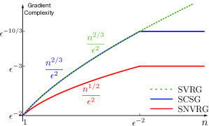
Figure 1: Comparison of gradient complexities.

Acceleration by high-order smoothness assumption With only Lipschitz continuous gradient assumption, Carmon et al. [9] showed that the lower bound for both deterministic and stochastic algorithms to achieve an $\epsilon$-approximate stationary point is $\Omega(\epsilon^{-2})$. With high-order smoothness assumptions, i.e., Hessian Lipschitzness, Hessian smoothness etc., a series of work have shown the existence of acceleration. For instance, Agarwal et al. [1] gave an algorithm based on Fast-PCA which can achieve an $\epsilon$-approximate stationary point with gradient complexity $\widetilde{O}(n\epsilon^{-3/2}+n^{3/4}\epsilon^{-7/4})$ Carmon et al. [7, 8] showed two algorithms based on finding exact or inexact negative curvature which can achieve an $\epsilon$-approximate stationary point with gradient complexity $\widetilde{O}(n\epsilon^{-7/4})$. In this work, we only consider gradient Lipschitz without assuming Hessian Lipschitz or Hessian smooth. Therefore, our result is not directly comparable to the methods in this category.

Acceleration by momentum The fact that using momentum is able to accelerate algorithms has been shown both in theory and practice in convex optimization [37, 31, 18, 23, 14, 32, 29, 2]. However, there is no evidence that such acceleration exists in nonconvex optimization with only Lipschitz continuous gradient assumption [15, 27, 36, 28, 24]. If $F$ satisfies $\lambda$-strongly nonconvex, i.e., $\nabla^{2}F\succeq-\lambda\mathbf{I}$, Allen-Zhu [3] proved that Natasha $1$, an algorithm based on nonconvex momentum, is able to find an $\epsilon$-approximate stationary point in $\widetilde{O}(n^{2/3}L^{2/3}\lambda^{1/3}\epsilon^{-2})$. Later, Allen-Zhu [3] further showed that Natasha 2, an online version of Natasha 1, is able to achieve an $\epsilon$-approximate stationary point within $\widetilde{O}(\epsilon^{-3.25})$ stochastic gradient evaluations.

After our paper was submitted to NIPS and released on arXiv, a paper [12] was released on arXiv after our work, which independently proposes a different algorithm and achieves the same convergence rate for finding an $\epsilon$-approximate stationary point.

To give a thorough comparison of our proposed algorithm with existing first-order algorithms for nonconvex finite-sum optimization, we summarize the gradient complexity of the most relevant algorithms in Table 1. We also plot the gradient complexities of different algorithms in Figure 1 for nonconvex smooth functions. Note that GD and SGD are always worse than SVRG and SCSG according to Table 1. In addition, GNC-AGD and Natasha2 needs additional Hessian Lipschitz condition. Therefore, we only plot the gradient complexity of SVRG, SCSG and our proposed SNVRG in Figure 1.

Table 1: Comparisons on gradient complexity of different algorithms. The second column shows the gradient complexity for a nonconvex and smooth function to achieve an $\epsilon$-approximate stationary point (i.e., $\|\nabla F(\mathbf{x})\|_{2}\leq\epsilon$). The third column presents the gradient complexity for a gradient dominant function to achieve an $\epsilon$-approximate global minimizer (i.e., $F(\mathbf{x})-\min_{\mathbf{x}}F(\mathbf{x})\leq\epsilon$). The last column presents the space complexity of all algorithms.

Algorithm	nonconvex	gradient dominant	Hessian Lipschitz
GD	$O\big{(}\frac{n}{\epsilon^{2}}\big{)}$	$\widetilde{O}(\tau n)$	No
SGD	$O\big{(}\frac{1}{\epsilon^{4}}\big{)}$	$O\big{(}\frac{1}{\epsilon^{4}}\big{)}$	No
SVRG [40]	$O\big{(}\frac{n^{2/3}}{\epsilon^{2}}\big{)}$	$\widetilde{O}(n+\tau n^{2/3})$	No
SCSG [26]	$O\big{(}\frac{1}{\epsilon^{10/3}}\land\frac{n^{2/3}}{\epsilon^{2}}\big{)}$	$\widetilde{O}\Big{(}n\wedge\frac{\tau}{\epsilon}+\tau\big{(}n\wedge\frac{\tau}{\epsilon}\big{)}^{2/3}\Big{)}$	No
GNC-AGD [8]	$\widetilde{O}\big{(}\frac{n}{\epsilon^{1.75}}\big{)}$	N/A	Needed
Natasha 2 [3]	$\widetilde{O}\big{(}\frac{1}{\epsilon^{3.25}}\big{)}$	N/A	Needed
SNVRG (this paper)	$\widetilde{O}\big{(}\frac{1}{\epsilon^{3}}\land\frac{n^{1/2}}{\epsilon^{2}}\big{)}$	$\widetilde{O}\Big{(}n\wedge\frac{\tau}{\epsilon}+\tau\big{(}n\wedge\frac{\tau}{\epsilon}\big{)}^{1/2}\Big{)}$	No

Notation: Let $\mathbf{A}=[A_{ij}]\in\mathbb{R}^{d\times d}$ be a matrix and $\mathbf{x}=(x_{1},...,x_{d})^{\top}\in\mathbb{R}^{d}$ be a vector. $\mathbf{I}$ denotes an identity matrix. We use $\|\mathbf{v}\|_{2}$ to denote the 2-norm of vector $\mathbf{v}\in\mathbb{R}^{d}$. We use $\langle\cdot,\cdot\rangle$ to represent the inner product of two vectors. Given two sequences $\{a_{n}\}$ and $\{b_{n}\}$, we write $a_{n}=O(b_{n})$ if there exists a constant $0<C<+\infty$ such that $a_{n}\leq C\,b_{n}$. We write $a_{n}=\Omega(b_{n})$ if there exists a constant $0<C<+\infty$, such that $a_{n}\geq C\,b_{n}$. We use notation $\widetilde{O}(\cdot)$ to hide logarithmic factors. We also make use of the notation $f_{n}\lesssim g_{n}$ ($f_{n}\gtrsim g_{n}$) if $f_{n}$ is less than (larger than) $g_{n}$ up to a constant. We use productive symbol $\prod_{i=a}^{b}c_{i}$ to denote $c_{a}c_{a+1}\dots c_{b}$. Moreover, if $a>b$, we take the product as 1. We use $\lfloor\cdot\rfloor$ as the floor function. We use $\log(x)$ to represent the logarithm of $x$ to base 2. $a\land b$ is a shorthand notation for $\min(a,b)$.

2 Preliminaries

In this section, we present some definitions that will be used throughout our analysis.

Definition 2.1.

A function $f$ is $L$-smooth, if for any $\mathbf{x},\mathbf{y}\in\mathbb{R}^{d}$, we have

$$\|\nabla f(\mathbf{x})-\nabla f(\mathbf{y})\|_{2}\leq L\|\mathbf{x}-\mathbf{y}\|_{2}.$$ (2.1)

Definition 2.1 implies that if $f$ is $L$-smooth, we have for any $\mathbf{x},\mathbf{h}\in\mathbb{R}^{d}$

$$f(\mathbf{x}+\mathbf{h})\leq f(\mathbf{x})+\langle\nabla f(\mathbf{x}),\mathbf{h}\rangle+\frac{L}{2}\|\mathbf{h}\|_{2}^{2}.$$ (2.2)

Definition 2.2.

A function $f$ is $\lambda$-strongly convex, if for any $\mathbf{x},\mathbf{y}\in\mathbb{R}^{d}$, we have

$$f(\mathbf{x}+\mathbf{h})\geq f(\mathbf{x})+\langle\nabla f(\mathbf{x}),\mathbf{h}\rangle+\frac{\lambda}{2}\|\mathbf{h}\|_{2}^{2}.$$ (2.3)

Definition 2.3.

A function $F$ with finite-sum structure in (1.1) is said to have stochastic gradients with bounded variance $\sigma^{2}$, if for any $\mathbf{x}\in\mathbb{R}^{d}$, we have

$$\mathbb{E}_{i}\|\nabla f_{i}(\mathbf{x})-\nabla F(\mathbf{x})\|_{2}^{2}\leq\sigma^{2},$$ (2.4)

where $i$ a random index uniformly chosen from $[n]$ and $\mathbb{E}_{i}$ denotes the expectation over such $i$.

$\sigma^{2}$ is called the upper bound on the variance of stochastic gradients [26].

Definition 2.4.

A function $F$ with finite-sum structure in (1.1) is said to have averaged $L$-Lipschitz gradient, if for any $\mathbf{x},\mathbf{y}\in\mathbb{R}^{d}$, we have

$$\mathbb{E}_{i}\|\nabla f_{i}(\mathbf{x})-\nabla f_{i}(\mathbf{y})\|_{2}^{2}\leq L^{2}\|\mathbf{x}-\mathbf{y}\|_{2}^{2},$$ (2.5)

where $i$ is a random index uniformly chosen from $[n]$ and $\mathbb{E}_{i}$ denotes the expectation over the choice.

Definition 2.5.

We say a function $f$ is lower-bounded by $f^{*}$ if for any $\mathbf{x}\in\mathbb{R}^{d}$, $f(\mathbf{x})\geq f^{*}$.

We also consider a class of functions namely gradient dominated functions [38], which is formally defined as follows:

Definition 2.6.

We say function $f$ is $\tau$-gradient dominated if for any $\mathbf{x}\in\mathbb{R}^{d}$, we have

$$f(\mathbf{x})-f(\mathbf{x}^{*})\leq\tau\cdot\|\nabla f(\mathbf{x})\|_{2}^{2},$$ (2.6)

where $\mathbf{x}^{*}\in\mathbb{R}^{d}$ is the global minimum of $f$.

Note that gradient dominated condition is also known as the Polyak-Lojasiewicz (P-L) condition [38], and is not necessarily convex. It is weaker than strong convexity as well as other popular conditions that appear in the optimization literature [20].

3 The Proposed Algorithm

In this section, we present our nested stochastic variance reduction algorithm, namely, SNVRG.

Algorithm 1 One-epoch-SNVRG($\mathbf{x}_{0}$, $F,K,M,\{T_{l}\},\{B_{l}\},B$)

1:  Input: initial point $\mathbf{x}_{0}$, function $F$, loop number $K$, step size parameter $M$, loop parameters $T_{l},l\in[K]$, batch parameters $B_{l},l\in[K]$, base batch size $B>0$.

2:  $\mathbf{x}^{(l)}_{0}\leftarrow\mathbf{x}_{0}$, $\mathbf{g}^{(l)}_{0}\leftarrow 0$, $0\leq l\leq K$

3:  Uniformly generate index set $I\subset[n]$ without replacement, $|I|=B$

4:  $\mathbf{g}^{(0)}_{0}\leftarrow 1/B\sum_{i\in I}\nabla f_{i}(\mathbf{x}_{0})$

5:  $\mathbf{v}_{0}\leftarrow\sum_{l=0}^{K}\mathbf{g}_{0}^{(l)}$

6:  $\mathbf{x}_{1}=\mathbf{x}_{0}-1/(10M)\cdot\mathbf{v}_{0}$

7:  for $t=1,...,\prod_{l=1}^{K}T_{l}-1$ do

8:     $r=\min\{j:0=(t\mod\prod_{l=j+1}^{K}T_{l}),\ 0\leq j\leq K\}$

9:     $\{\mathbf{x}^{(l)}_{t}\}\leftarrow\text{Update\_reference\_points}(\{\mathbf{x}^{(l)}_{t-1}\},\mathbf{x}_{t},r),0\leq l\leq K$.

10:     $\{\mathbf{g}_{t}^{(l)}\}\leftarrow\text{Update\_reference\_gradients}(\{\mathbf{g}^{(l)}_{t-1}\},\{\mathbf{x}^{(l)}_{t}\},r),0\leq l\leq K$.

11:     $\mathbf{v}_{t}\leftarrow\sum_{l=0}^{K}\mathbf{g}_{t}^{(l)}$

12:     $\mathbf{x}_{t+1}\leftarrow\mathbf{x}_{t}-1/(10M)\cdot\mathbf{v}_{t}$

13:  end for

14:  $\mathbf{x}_{\text{out}}\leftarrow$ uniformly random choice from $\{\mathbf{x}_{t}\}$, where $0\leq t<\prod_{l=1}^{K}T_{l}$

15:  $T=\prod_{l=1}^{K}T_{l}$

16:  Output: $[\mathbf{x}_{\text{out}},\mathbf{x}_{T}]$

17:  Function: Update_reference_points($\{\mathbf{x}_{\text{old}}^{(l)}\},\mathbf{x},r$)

18:  $\mathbf{x}_{\text{new}}^{(l)}\leftarrow\mathbf{x}_{\text{old}}^{(l)},0\leq l\leq r-1$; $\mathbf{x}_{\text{new}}^{(l)}\leftarrow\mathbf{x},r\leq l\leq K$

19:  return  $\{\mathbf{x}_{\text{new}}^{(l)}\}$

20:  Function: Update_reference_gradients($\{\mathbf{g}^{(l)}_{\text{old}}\},\{\mathbf{x}^{(l)}_{\text{new}}\},r$)

21:  $\mathbf{g}^{(l)}_{\text{new}}\leftarrow\mathbf{g}^{(l)}_{\text{old}},0\leq l<r$

22:  for $r\leq l\leq K$ do

23:     Uniformly generate index set $I\subset[n]$ without replacement, $|I|=B_{l}$

24:     $\mathbf{g}_{\text{new}}^{(l)}\leftarrow 1/B_{l}\sum_{i\in I}\big{[}\nabla f_{i}(\mathbf{x}^{(l)}_{\text{new}})-\nabla f_{i}(\mathbf{x}^{(l-1)}_{\text{new}})\big{]}$

25:  end for

26:  return  $\{\mathbf{g}_{\text{new}}^{(l)}\}$.

One-epoch-SNVRG: We first present the key component of our main algorithm, One-epoch-SNVRG, which is displayed in Algorithm 1. The most innovative part of Algorithm 1 attributes to the $K+1$ reference points and $K+1$ reference gradients. Note that when $K=1$, Algorithm 1 reduces to one epoch of SVRG algorithm [19, 40, 5]. To better understand our One-epoch SNVRG algorithm, it would be helpful to revisit the original SVRG which is a special case of our algorithm. For the finite-sum optimization problem in (1.1), the original SVRG takes the following updating formula

$$\mathbf{x}_{t+1}=\mathbf{x}_{t}-\eta\mathbf{v}_{t}=\mathbf{x}_{t}-\eta\big{(}\nabla F(\widetilde{\mathbf{x}})+\nabla f_{i_{t}}(\mathbf{x}_{t})-\nabla f_{i_{t}}(\widetilde{\mathbf{x}})\big{)},$$

where $\eta>0$ is the step size, $i_{t}$ is a random index uniformly chosen from $[n]$ and $\widetilde{\mathbf{x}}$ is a snapshot for $\mathbf{x}_{t}$ after every $T_{1}$ iterations. There are two reference points in the update formula at $\mathbf{x}_{t}$: $\mathbf{x}_{t}^{(0)}=\widetilde{\mathbf{x}}$ and $\mathbf{x}_{t}^{(1)}=\mathbf{x}_{t}$. Note that $\widetilde{\mathbf{x}}$ is updated every $T_{1}$ iterations, namely, $\widetilde{\mathbf{x}}$ is set to be $\mathbf{x}_{t}$ only when $(t\mod T_{1})=0$. Moreover, in the semi-stochastic gradient $\mathbf{v}_{t}$, there are also two reference gradients and we denote them by $\mathbf{g}_{t}^{(0)}=\nabla F(\widetilde{\mathbf{x}})$ and $\mathbf{g}_{t}^{(1)}=\nabla f_{i_{t}}(\mathbf{x}_{t})-\nabla f_{i_{t}}(\widetilde{\mathbf{x}})=\nabla f_{i_{t}}(\mathbf{x}_{t}^{(1)})-\nabla f_{i_{t}}(\mathbf{x}_{t}^{(0)})$.

Back to our One-epoch-SNVRG, we can define similar reference points and reference gradients as that in the special case of SVRG. Specifically, for $t=0,\ldots,\prod_{l=1}^{K}T_{l}-1$, each point $\mathbf{x}_{t}$ has $K+1$ reference points $\{\mathbf{x}_{t}^{(l)}\},l=0,\ldots,K$, which is set to be $\mathbf{x}_{t}^{(l)}=\mathbf{x}_{t^{l}}$ with index $t^{l}$ defined as

$$t^{l}=\bigg{\lfloor}\frac{t}{\prod_{k=l+1}^{K}T_{k}}\bigg{\rfloor}\cdot\prod_{k=l+1}^{K}T_{k}.$$ (3.1)

Specially, note that we have $\mathbf{x}_{t}^{(0)}=\mathbf{x}_{0}$ and $\mathbf{x}_{t}^{(K)}=\mathbf{x}_{t}$ for all $t=0,\ldots,\prod_{l=1}^{K}T_{l}-1$. Similarly, $\mathbf{x}_{t}$ also has $K+1$ reference gradients $\{\mathbf{g}_{t}^{(l)}\}$, which can be defined based on the reference points $\{\mathbf{x}_{t}^{(l)}\}$:

$$\begin{split}&\mathbf{g}_{t}^{(0)}=\frac{1}{B}\sum_{i\in I}\nabla f_{i}(\mathbf{x}_{0}),\qquad\mathbf{g}_{t}^{(l)}=\frac{1}{B_{l}}\sum_{i\in{I_{l}}}\big{[}\nabla f_{i}(\mathbf{x}_{t}^{(l)})-\nabla f_{i}(\mathbf{x}_{t}^{(l-1)})\big{]},l=1,\ldots,K,\end{split}$$ (3.2)

where $I,I_{l}$ are random index sets with $|I|=B,|I_{l}|=B_{l}$ and are uniformly generated from $[n]$ without replacement. Based on the reference points and reference gradients, we then update $\mathbf{x}_{t+1}=\mathbf{x}_{t}-1/(10M)\cdot\mathbf{v}_{t}$, where $\mathbf{v}_{t}=\sum_{l=0}^{K}\mathbf{g}_{t}^{(l)}$ and $M$ is the step size parameter. The illustration of reference points and gradients of SNVRG is displayed in Figure 2.

We remark that it would be a huge waste for us to re-evaluate $\mathbf{g}_{t}^{(l)}$ at each iteration. Fortunately, due to the fact that each reference point is only updated after a long period, we can maintain $\mathbf{g}_{t}^{(l)}=\mathbf{g}_{t-1}^{(l)}$ and only need to update $\mathbf{g}_{t}^{(l)}$ when $\mathbf{x}_{t}^{(l)}$ has been updated as is suggested by Line 24 in Algorithm 1.

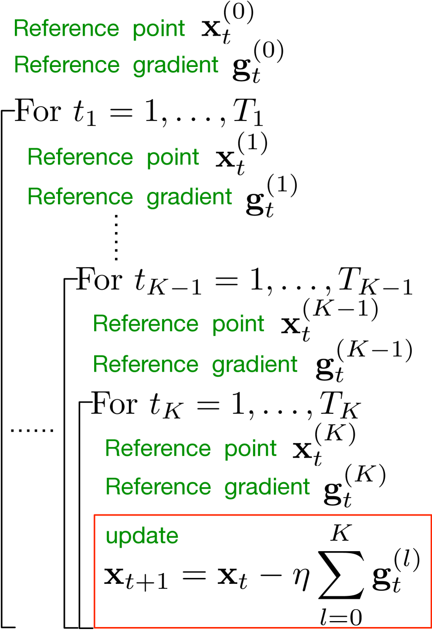
Figure 2: Illustration of reference points and gradients.

SNVRG: Using One-epoch-SNVRG (Algorithm 1) as a building block, we now present our main algorithm: Algorithm 2 for nonconvex finite-sum optimization to find an $\epsilon$-approximate stationary point. At each iteration of Algorithm 2, it executes One-epoch-SNVRG (Algorithm 1) which takes $\mathbf{z}_{s-1}$ as its input and outputs $[\mathbf{y}_{s},\mathbf{z}_{s}]$. We choose $\mathbf{y}_{\text{out}}$ as the output of Algorithm 2 uniformly from $\{\mathbf{y}_{s}\}$, for $s=1,\ldots,S$.

SNVRG-PL: In addition, when function $F$ in (1.1) is gradient dominated as defined in Definition 2.6 (P-L condition), it has been proved that the global minimum can be found by SGD [20], SVRG [40] and SCSG [26] very efficiently. Following a similar trick used in [40], we present Algorithm 3 on top of Algorithm 2, to find the global minimum in this setting. We call Algorithm 3 SNVRG-PL, because gradient dominated condition is also known as Polyak-Lojasiewicz (PL) condition [38].

Space complexity: We briefly compare the space complexity between our algorithms and other variance reduction based algorithms. SVRG and SCSG needs $O(d)$ space complexity to store one reference gradient, SAGA [10] needs to store reference gradients for each component functions, and its space complexity is $O(nd)$ without using any trick. For our algorithm SNVRG, we need to store $K$ reference gradients, thus its space complexity is $O(Kd)$. In our theory, we will show that $K=O(\log\log n)$. Therefore, the space complexity of our algorithm is actually $\widetilde{O}(d)$, which is almost comparable to that of SVRG and SCSG.

Algorithm 2 SNVRG

1:  Input: initial point $\mathbf{z}_{0}$, function $F$, $K$, $M$, $\{T_{l}\}$, $\{B_{l}\}$, batch $B$, $S$.

2:  for $s=1,\dots,S$ do

3:     denote $\mathcal{P}=(F,K,M,\{T_{l}\},\{B_{l}\},B)$

4:     $[\mathbf{y}_{s},\mathbf{z}_{s}]$ $\leftarrow$$\text{One-epoch-}\text{SNVRG}(\mathbf{z}_{s-1},\mathcal{P})$

5:  end for

6:  Output: Uniformly choose $\mathbf{y}_{\text{out}}$ from $\{\mathbf{y}_{s}\}$.

Algorithm 3 SNVRG-PL

1:  Input: initial point $\mathbf{z}_{0}$, function $F$, $K$, $M$, $\{T_{l}\}$, $\{B_{l}\}$, batch $B$, $S$, $U$.

2:  for $u=1,\dots,U$ do

3:     denote $\mathcal{Q}=(F,K,M,\{T_{l}\},\{B_{l}\},B,S)$

4:     $\mathbf{z}_{u}=\text{SNVRG}(\mathbf{z}_{u-1},\mathcal{Q})$

5:  end for

6:  Output: $\mathbf{z}_{\text{out}}=\mathbf{z}_{U}$.

4 Main Theory

In this section, we provide the convergence analysis of SNVRG.

4.1 Convergence of SNVRG

We first analyze One-epoch-SNVRG (Algorithm 1) and provide a particular choice of parameters.

Lemma 4.1.

Suppose that $F$ has averaged $L$-Lipschitz gradient, in Algorithm 1, suppose $B\geq 2$ and let the number of nested loops be $K=\log\log B$. Choose the step size parameter as $M=6L$. For the loop and batch parameters, let $T_{1}=2,B_{1}=6^{K}\cdot B$ and

$$T_{l}=2^{2^{l-2}},\qquad B_{l}=6^{K-l+1}\cdot B/2^{2^{l-1}},$$

for all $2\leq l\leq K$. Then the output of Algorithm 1 $[\mathbf{x}_{\text{out}},\mathbf{x}_{T}]$ satisfies

$$\mathbb{E}\|\nabla F(\mathbf{x}_{\text{out}})\|_{2}^{2}\leq C\bigg{(}\frac{L}{B^{1/2}}\cdot\mathbb{E}\big{[}F(\mathbf{x}_{0})-F(\mathbf{x}_{T})\big{]}+\frac{\sigma^{2}}{B}\cdot\operatorname{\mathds{1}}(B<n)\bigg{)}$$ (4.1)

within $1\lor(7B\log^{3}B)$ stochastic gradient computations, where $T=\prod_{l=1}^{K}T_{l}$, $C=600$ is a constant and $\operatorname{\mathds{1}}(\cdot)$ is the indicator function.

The following theorem shows the gradient complexity for Algorithm 2 to find an $\epsilon$-approximate stationary point with a constant base batch size $B$.

Theorem 4.2.

Suppose that $F$ has averaged $L$-Lipschitz gradient and stochastic gradients with bounded variance $\sigma^{2}$. In Algorithm 2, let $B=n\land(2C\sigma^{2}/\epsilon^{2})$ , $S=1\lor(2CL\Delta_{F}/(B^{1/2}\epsilon^{2}))$ and $C=600$. The rest parameters $(K,M,\{B_{l}\},\{T_{l}\})$ are chosen the same as in Lemma 4.1. Then the output $\mathbf{y}_{\text{out}}$ of Algorithm 2 satisfies $\mathbb{E}\|\nabla F(\mathbf{y}_{\text{out}})\|_{2}^{2}\leq\epsilon^{2}$ with less than

$$O\bigg{(}\log^{3}\bigg{(}\frac{\sigma^{2}}{\epsilon^{2}}\land n\bigg{)}\bigg{[}\frac{\sigma^{2}}{\epsilon^{2}}\land n+\frac{L\Delta_{F}}{\epsilon^{2}}\bigg{[}\frac{\sigma^{2}}{\epsilon^{2}}\land n\bigg{]}^{1/2}\bigg{]}\bigg{)}$$ (4.2)

stochastic gradient computations, where $\Delta_{F}=F(\mathbf{z}_{0})-F^{*}$.

Remark 4.3.

If we treat $\sigma^{2},L$ and $\Delta_{F}$ as constants, and assume $\epsilon\ll 1$, then (4.2) can be simplified to $\widetilde{O}(\epsilon^{-3}\land n^{1/2}\epsilon^{-2})$. This gradient complexity is strictly better than $O(\epsilon^{-10/3}\land n^{2/3}\epsilon^{-2})$, which is achieved by SCSG [26]. Specifically, when $n\lesssim 1/\epsilon^{2}$, our proposed SNVRG is faster than SCSG by a factor of $n^{1/6}$; when $n\gtrsim 1/\epsilon^{2}$, SNVRG is faster than SCSG by a factor of $\epsilon^{-1/3}$. Moreover, SNVRG also outperforms Natasha 2 [3] which attains $\widetilde{O}(\epsilon^{-3.25})$ gradient complexity and needs the additional Hessian Lipschitz condition.

4.2 Convergence of SNVRG-PL

We now consider the case when $F$ is a $\tau$-gradient dominated function. In general, we are able to find an $\epsilon$-approximate global minimizer of $F$ instead of only an $\epsilon$-approximate stationary point. Algorithm 3 uses Algorithm 2 as a component.

Theorem 4.4.

Suppose that $F$ has averaged $L$-Lipschitz gradient and stochastic gradients with bounded variance $\sigma^{2}$, $F$ is a $\tau$-gradient dominated function. In Algorithm 3, let the base batch size $B=n\land(4C_{1}\tau\sigma^{2}/\epsilon)$, the number of epochs for SNVRG $S=1\lor(2C_{1}\tau L/B^{1/2})$ and the number of epochs $U=\log(2\Delta_{F}/\epsilon)$. The rest parameters $(K,M,\{B_{l}\},\{T_{l}\})$ are chosen as the same in Lemma 4.1. Then the output $\mathbf{z}_{\text{out}}$ of Algorithm 3 satisfies $\mathbb{E}\big{[}F(\mathbf{z}_{\text{out}})-F^{*}\big{]}\leq\epsilon$ within

$$O\bigg{(}\log^{3}\bigg{(}n\land\frac{\tau\sigma^{2}}{\epsilon}\bigg{)}\log\frac{\Delta_{F}}{\epsilon}\bigg{[}n\land\frac{\tau\sigma^{2}}{\epsilon}+\tau L\bigg{[}n\land\frac{\tau\sigma^{2}}{\epsilon}\bigg{]}^{1/2}\bigg{]}\bigg{)}$$ (4.3)

stochastic gradient computations, where $\Delta_{F}=F(\mathbf{z}_{0})-F^{*}$

Remark 4.5.

If we treat $\sigma^{2}$, $L$ and $\Delta_{F}$ as constants, then the gradient complexity in (4.3) turns into $\widetilde{O}(n\land\tau\epsilon^{-1}+\tau(n\land\tau\epsilon^{-1})^{1/2})$. Compared with nonconvex SVRG [41] which achieves $\widetilde{O}(n+\tau n^{2/3})$ gradient complexity, our SNVRG-PL is strictly better than SVRG in terms of the first summand and is faster than SVRG at least by a factor of $n^{1/6}$ in terms of the second summand. Compared with a more general variant of SVRG, namely, the SCSG algorithm [26], which attains $\widetilde{O}\big{(}n\wedge\tau\epsilon^{-1}+\tau(n\wedge\tau\epsilon^{-1})^{2/3}\big{)}$ gradient complexity, SNVRG-PL also outperforms it by a factor of $(n\land\tau\epsilon^{-1})^{1/6}$.

If we further assume that $F$ is $\lambda$-strongly convex, then it is easy to verify that $F$ is also $1/(2\lambda)$-gradient dominated. As a direct consequence, we have the following corollary:

Corollary 4.6.

Under the same conditions and parameter choices as Theorem 4.4. If we additionally assume that $F$ is $\lambda$-strongly convex, then Algorithm 3 will outputs an $\epsilon$-approximate global minimizer within

$$\widetilde{O}\bigg{(}n\land\frac{\lambda\sigma^{2}}{\epsilon}+\kappa\cdot\bigg{[}n\land\frac{\lambda\sigma^{2}}{\epsilon}\bigg{]}^{1/2}\bigg{)}$$ (4.4)

stochastic gradient computations, where $\kappa=L/\lambda$ is the condition number of $F$.

Remark 4.7.

Corollary 4.6 suggests that when we regard $\lambda$ and $\sigma^{2}$ as constants and set $\epsilon\ll 1$, Algorithm 3 is able to find an $\epsilon$-approximate global minimizer within $\widetilde{O}(n+n^{1/2}\kappa)$ stochastic gradient computations, which matches SVRG-lep in Katyusha X [4]. Using catalyst techniques [29] or Katyusha momentum [2], it can be further accelerated to $\widetilde{O}(n+n^{3/4}\sqrt{\kappa})$, which matches the best-known convergence rate [45, 4].

5 Experiments

In this section, we compare our algorithm SNVRG with other baseline algorithms on training a convolutional neural network for image classification. We compare the performance of the following algorithms: SGD; SGD with momentum [39] (denoted by SGD-momentum); ADAM[21]; SCSG [26]. It is worth noting that SCSG is a special case of SNVRG when the number of nested loops $K=1$. Due to the memory cost, we did not compare GD and SVRG which need to calculate the full gradient. Although our theoretical analysis holds for general $K$ nested loops, it suffices to choose $K=2$ in SNVRG to illustrate the effectiveness of the nested structure for the simplification of implementation. In this case, we have $3$ reference points and gradients. All experiments are conducted on Amazon AWS p2.xlarge servers which comes with Intel Xeon E5 CPU and NVIDIA Tesla K80 GPU (12G GPU RAM). All algorithm are implemented in Pytorch platform version $0.4.0$ within Python $3.6.4$.

Datasets We use three image datasets: (1) The MNIST dataset [44] consists of handwritten digits and has $50,000$ training examples and $10,000$ test examples. The digits have been size-normalized to fit the network, and each image is 28 pixels by 28 pixels. (2) CIFAR10 dataset [22] consists of images in 10 classes and has $50,000$ training examples and $10,000$ test examples. The digits have been size-normalized to fit the network, and each image is 32 pixels by 32 pixels. (3) SVHN dataset [33] consists of images of digits and has $531,131$ training examples and $26,032$ test examples. The digits have been size-normalized to fit the network, and each image is 32 pixels by 32 pixels.

CNN Architecture We use the standard LeNet [25], which has two convolutional layers with 6 and 16 filters of size 5 respectively, followed by three fully-connected layers with output size 120, 84 and 10. We apply max pooling after each convolutional layer.

Implementation Details & Parameter Tuning We did not use the random data augmentation which is set as default by Pytorch, because it will apply random transformation (e.g., clip and rotation) at the beginning of each epoch on the original image dataset, which will ruin the finite-sum structure of the loss function. We set our grid search rules for all three datasets as follows. For SGD, we search the batch size from $\{256,512,1024,2048\}$ and the initial step sizes from $\{1,0.1,0.01\}$. For SGD-momentum, we set the momentum parameter as $0.9$. We search its batch size from $\{256,512,1024,2048\}$ and the initial learning rate from $\{1,0.1,0.01\}$. For ADAM, we search the batch size from $\{256,512,1024,2048\}$ and the initial learning rate from $\{0.01,0.001,0.0001\}$. For SCSG and SNVRG, we choose loop parameters $\{T_{l}\}$ which satisfy $B_{l}\cdot\prod_{j=1}^{l}T_{j}=B$ automatically. In addition, for SCSG, we set the batch sizes $(B,B_{1})=(B,B/b)$, where $b$ is the batch size ratio parameter. We search $B$ from $\{256,512,1024,2048\}$ and we search $b$ from $\{2,4,8\}$. We search its initial learning rate from $\{1,0.1,0.01\}$. For our proposed SNVRG, we set the batch sizes $(B,B_{1},B_{2})=(B,B/b,B/b^{2})$, where $b$ is the batch size ratio parameter. We search $B$ from $\{256,512,1024,2048\}$ and $b$ from $\{2,4,8\}$. We search its initial learning rate from $\{1,0.1,0.01\}$. Following the convention of deep learning practice, we apply learning rate decay schedule to each algorithm with the learning rate decayed by $0.1$ every 20 epochs. We also conducted experiments based on plain implementation of different algorithms without learning rate decay, which is deferred to the appendix.

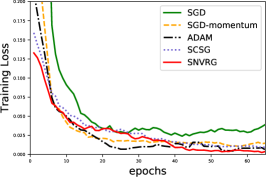
(a) training loss (MNIST)

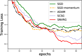
(b) training loss (CIFAR10)

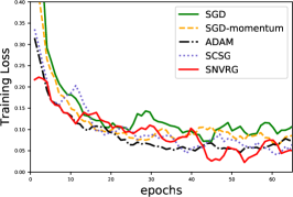
(c) training loss (SVHN)

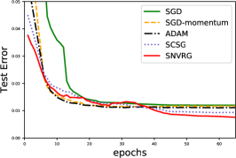
(d) test error (MNIST)

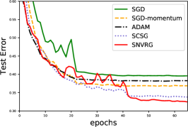
(e) test error (CIFAR10)

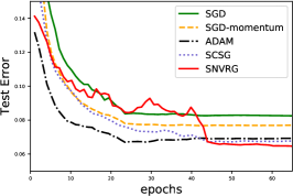
(f) test error (SVHN)

Figure 3: Experiment results on different datasets with learning rate decay. (a) and (d) depict the training loss and test error (top-1 error) v.s. data epochs for training LeNet on MNIST dataset. (b) and (e) depict the training loss and test error v.s. data epochs for training LeNet on CIFAR10 dataset. (c) and (f) depict the training loss and test error v.s. data epochs for training LeNet on SVHN dataset.

We plotted the training loss and test error for different algorithms on each dataset in Figure 3. The results on MNIST are presented in Figures 3(a) and 3(d); the results on CIFAR10 are in Figures 3(b) and 3(e); and the results on SVHN dataset are shown in Figures 3(c) and 3(f). It can be seen that with learning rate decay schedule, our algorithm SNVRG outperforms all baseline algorithms, which confirms that the use of nested reference points and gradients can accelerate the nonconvex finite-sum optimization.

We would like to emphasize that, while this experiment is on training convolutional neural networks, the major goal of this experiment is to illustrate the advantage of our algorithm and corroborate our theory, rather than claiming a state-of-the-art algorithm for training deep neural networks.

6 Conclusions and Future Work

In this paper, we proposed a stochastic nested variance reduced gradient method for finite-sum nonconvex optimization. It achieves substantially better gradient complexity than existing first-order algorithms. This partially resolves a long standing question that whether the dependence of gradient complexity on $n$ for nonconvex SVRG and SCSG can be further improved. There is still an open question: whether $\widetilde{O}(n\land\epsilon^{-2}+\epsilon^{-3}\land n^{1/2}\epsilon^{-2})$ is the optimal gradient complexity for finite-sum and stochastic nonconvex optimization problem? For finite-sum nonconvex optimization problem, the lower bound has been proved in Fang et al. [12], which suggests that our algorithm is near optimal up to a logarithmic factor. However, for general stochastic problem, the lower bound is still unknown. We plan to derive such lower bound in our future work. On the other hand, our algorithm can also be extended to deal with nonconvex nonsmooth finite-sum optimization using proximal gradient [42].

Appendix A Proof of the Main Theoretical Results

In this section, we provide the proofs of our main theories in Section 4.

A.1 Proof of Lemma 4.1

We first prove our key lemma on One-epoch-SNVRG. In order to prove Lemma 4.1, we need the following supporting lemma:

Lemma A.1.

Let $T=\prod_{l=1}^{K}T_{l}$. If the step size and batch size parameters in Algorithm 1 satisfy $M\geq 6L$ and $B_{l}\geq 6^{K-l+1}(\prod_{s=l}^{K}T_{s})^{2}$, then the output of Algorithm 1 satisfies

$$\mathbb{E}\|\nabla F(\mathbf{x}_{\text{out}})\|_{2}^{2}\leq C\bigg{(}\frac{M}{T}\cdot\mathbb{E}\big{[}F(\mathbf{x}_{0})-F(\mathbf{x}_{T})\big{]}+\frac{2\sigma^{2}}{B}\cdot\operatorname{\mathds{1}}(B<n)\bigg{)},$$ (A.1)

where $C=100$ is a constant.

Proof of Lemma 4.1.

Note that $B=2^{2^{K}}$, we can easily check that the choice of $M,\{T_{l}\},\{B_{l}\}$ in Lemma 4.1 satisfies the assumption of Lemma A.1. Moreover, we have

$$T=\prod_{l=1}^{K}T_{l}=B^{1/2}.$$ (A.2)

We now submit (A.2) into (A.1), which immediately implies (4.1).

Next we compute how many stochastic gradient computations we need in total after we run One-epoch-SNVRG once. According to the update of reference gradients in Algorithm 1, we only update $\mathbf{g}_{t}^{(0)}$ once at the beginning of Algorithm 1 (Line 4), which needs $B$ stochastic gradient computations. For $\mathbf{g}_{t}^{(l)}$, we only need to update it when $0=(t\mod\prod_{j=l+1}^{K}T_{j})$, and thus we need to sample $\mathbf{g}_{t}^{(l)}$ for $T/\prod_{j=l+1}^{K}T_{j}=\prod_{j=1}^{l}T_{j}$ times. We need $2B_{l}$ stochastic gradient computations for each sampling procedure (Line 24 in Algorithm 1). We use ${\mathcal{T}}$ to represent the total number of stochastic gradient computations, then based on above arguments we have

$${\mathcal{T}} =B+2\sum_{l=1}^{K}B_{l}\cdot\prod_{j=1}^{l}T_{j}.$$ (A.3)

Now we calculate ${\mathcal{T}}$ under the parameter choice of Lemma 4.1. Note that we can easily verify the following results:

$$\prod_{j=1}^{l}T_{j} =2^{2^{l-1}}=B^{\frac{2^{l}}{2^{K+1}}},\ B_{1}\cdot\prod_{j=1}^{1}T_{j}=2\times 6^{K}B,\ B_{l}\cdot\prod_{j=1}^{l}T_{j}=6^{K-l+1}B.$$ (A.4)

Submit (A.4) into (A.3) yields the following results:

$${\mathcal{T}} =B+2\bigg{(}2\times 6^{K}B+\sum_{l=2}^{K}6^{K-l+1}B\bigg{)}$$

$$<B+6\times 6^{K}B$$

$$=B+6\times 6^{\log\log B}B$$

$$<B+6B\log^{3}B.$$ (A.5)

Therefore, the total gradient complexity ${\mathcal{T}}$ is bounded as follows.

$${\mathcal{T}} \leq B+6B\log^{3}B\leq 7B\log^{3}B.$$ (A.6)

∎

A.2 Proof of Theorem 4.2

Now we prove our main theorem which spells out the gradient complexity of SNVRG.

Proof of Theorem 4.2.

By (4.1) we have

$$\mathbb{E}\|\nabla F(\mathbf{y}_{s})\|_{2}^{2}\leq C\bigg{(}\frac{L}{B^{1/2}}\cdot\mathbb{E}\big{[}F(\mathbf{z}_{s-1})-F(\mathbf{z}_{s})\big{]}+\frac{\sigma^{2}}{B}\cdot\operatorname{\mathds{1}}(B<n)\bigg{)},$$ (A.7)

where $C=600$. Taking summation for (A.7) over $s$ from $1$ to $S$, we have

$$\sum_{s=1}^{S}\mathbb{E}\|\nabla F(\mathbf{y}_{s})\|_{2}^{2} \leq C\bigg{(}\frac{L}{B^{1/2}}\cdot\mathbb{E}\big{[}F(\mathbf{z}_{0})-F(\mathbf{z}_{S})\big{]}+\frac{\sigma^{2}}{B}\cdot\operatorname{\mathds{1}}(B<n)\cdot S\bigg{)}.$$ (A.8)

Dividing both sides of (A.8) by $S$, we immediately obtain

$$\mathbb{E}\|\nabla F(\mathbf{y}_{\text{out}})\|_{2}^{2} \leq C\bigg{(}\frac{L\mathbb{E}\big{[}F(\mathbf{z}_{0})-F^{*}\big{]}}{SB^{1/2}}+\frac{\sigma^{2}}{B}\cdot\operatorname{\mathds{1}}(B<n)\bigg{)}$$ (A.9)

$$=C\bigg{(}\frac{L\Delta_{F}}{SB^{1/2}}+\frac{\sigma^{2}}{B}\cdot\operatorname{\mathds{1}}(B<n)\bigg{)},$$ (A.10)

where (A.9) holds because $F(\mathbf{z}_{S})\geq F^{*}$ and by the definition $\Delta_{F}=F(\mathbf{z}_{0})-F^{*}$. By the choice of parameters in Theorem 4.2, we have $B=n\land(2C\sigma^{2}/\epsilon^{2}),S=1\lor(2CL\Delta_{F}/(B^{1/2}\epsilon^{2}))$, which implies

$$\begin{split}\operatorname{\mathds{1}}(B<n)\cdot\sigma^{2}/B&\leq\epsilon^{2}/(2C),\quad\text{and}\quad L\Delta_{F}/(SB^{1/2})\leq\epsilon^{2}/(2C).\end{split}$$ (A.11)

Submitting (A.11) into (A.10), we have $\mathbb{E}\|\nabla F(\mathbf{y}_{\text{out}})\|_{2}^{2}\leq 2C\epsilon^{2}/(2C)=\epsilon^{2}$. By Lemma 4.1, we have that each One-epoch-SNVRG takes less than $7B\log^{3}B$ stochastic gradient computations. Since we have total $S$ epochs, so the total gradient complexity of Algorithm 2 is less than

$$S\cdot 7B\log^{3}B \leq 7B\log^{3}B+\frac{L\Delta_{F}}{\epsilon^{2}}\cdot 7B^{1/2}\log^{3}B$$

$$=O\bigg{(}\log^{3}\bigg{(}\frac{\sigma^{2}}{\epsilon^{2}}\land n\bigg{)}\bigg{[}\frac{\sigma^{2}}{\epsilon^{2}}\land n+\frac{L\Delta_{F}}{\epsilon^{2}}\bigg{[}\frac{\sigma^{2}}{\epsilon^{2}}\land n\bigg{]}^{1/2}\bigg{]}\bigg{)},$$ (A.12)

which leads to the conclusion. ∎

A.3 Proof of Theorem 4.4

We then prove the main theorem on gradient complexity of SNVRG under gradient dominance condition (Algorithm 3).

Proof of Theorem 4.4.

Following the proof of Theorem 4.2, we obtain a similar inequality with (A.9):

$$\mathbb{E}\|\nabla F(\mathbf{z}_{u+1})\|_{2}^{2}\leq C\bigg{(}\frac{L\mathbb{E}[F(\mathbf{z}_{u})-F^{*}]}{SB^{1/2}}+\frac{\sigma^{2}}{B}\cdot\operatorname{\mathds{1}}(B<n)\bigg{)}.$$ (A.13)

Since $F$ is a $\tau$-gradient dominated function, we have $\mathbb{E}\|\nabla F(\mathbf{z}_{u+1})\|_{2}^{2}\geq 1/\tau\cdot\mathbb{E}[F(\mathbf{z}_{u+1})-F^{*}]$ by Definition 2.6. Plugging this inequality into (A.13) yields

$$\mathbb{E}\big{[}F(\mathbf{z}_{u+1})-F^{*}\big{]} \leq\frac{C\tau L}{SB^{1/2}}\cdot\mathbb{E}\big{[}F(\mathbf{z}_{u})-F^{*}\big{]}+\frac{C\tau\sigma^{2}}{B}\cdot\operatorname{\mathds{1}}(B<n)$$

$$\leq\frac{1}{2}\mathbb{E}\big{[}F(\mathbf{z}_{u})-F^{*}\big{]}+\frac{\epsilon}{4},$$ (A.14)

where the second inequality holds due to the choice of parameters $B=n\land(4C_{1}\tau\sigma^{2}/\epsilon)$ and $S=1\lor(2C_{1}\tau L/B^{1/2})$ for Algorithm 3 in Theorem 4.4. By (A.14) we can derive

$$\mathbb{E}\big{[}F(\mathbf{z}_{u+1})-F^{*}\big{]}-\frac{\epsilon}{2}\leq\frac{1}{2}\bigg{(}\mathbb{E}\big{[}F(\mathbf{z}_{u})-F^{*}\big{]}-\frac{\epsilon}{2}\bigg{)},$$

which immediately implies

$$\mathbb{E}\big{[}F(\mathbf{z}_{U})-F^{*}\big{]}-\frac{\epsilon}{2}\leq\frac{1}{2^{U}}\bigg{(}\Delta_{F}-\frac{\epsilon}{2}\bigg{)}\leq\frac{\Delta_{F}}{2^{U}}.$$ (A.15)

Plugging the number of epochs $U=\log(2\Delta_{F}/\epsilon)$ into (A.15), we obtain $\mathbb{E}\big{[}F(\mathbf{z}_{U})-F^{*}\big{]}\leq\epsilon$. Note that each epoch of Algorithm 3 needs at most $S\cdot 7B\log^{3}B$ stochastic gradient computations by Theorem 4.2 and Algorithm 3 has $U$ epochs, which implies the total stochastic gradient complexity

$$U\cdot S\cdot 7B\log^{3}B =O\bigg{(}\log^{3}\bigg{(}n\land\frac{\tau\sigma^{2}}{\epsilon}\bigg{)}\log\frac{\Delta_{F}}{\epsilon}\bigg{[}n\land\frac{\tau\sigma^{2}}{\epsilon}+\tau L\bigg{[}n\land\frac{\tau\sigma^{2}}{\epsilon}\bigg{]}^{1/2}\bigg{]}\bigg{)}.$$ (A.16)

∎

Appendix B Proof of Key Lemma A.1

In this section, we focus on proving Lemma A.1 which plays a pivotal role in proving our main theorems. Let $M,\{T_{i}\},\{B_{i}\},B$ be the parameters as defined in Algorithm 1. We denote $T=\prod_{l=1}^{K}T_{l}$. We define filtration $\mathcal{F}_{t}=\sigma(\mathbf{x}_{0},\dots,\mathbf{x}_{t})$. Let $\{\mathbf{x}_{t}^{(l)}\},\{\mathbf{g}_{t}^{(l)}\}$ be the reference points and reference gradients in Algorithm 1. We define $\mathbf{v}_{t}^{(l)}$ as

$$\mathbf{v}_{t}^{(l)}:=\sum_{j=0}^{l}\mathbf{g}_{t}^{(j)},\quad\text{for }0\leq l\leq K.$$ (B.1)

We first present the following definition and two technical lemmas for the purpose of our analysis.

Definition B.1.

We define constant series $\{c^{(s)}_{j}\}$ as the following. For each $s$, we define $c^{(s)}_{T_{s}}$ as

$$c^{(s)}_{T_{s}} =\frac{M}{6^{K-s+1}\prod_{l=s}^{K}T_{l}}.$$ (B.2)

When $0\leq j<T_{s}$, we define $c^{(s)}_{j}$ by induction:

$$c^{(s)}_{j} =\bigg{(}1+\frac{1}{T_{s}}\bigg{)}c^{(s)}_{j+1}+\frac{3L^{2}}{M}\cdot\frac{\prod_{l=s+1}^{K}T_{l}}{B_{s}}.$$ (B.3)

Lemma B.2.

For any $p,s$, where $1\leq s\leq K$ and $0\leq p\prod_{j=s}^{K}T_{j}<(p+1)\prod_{j=s}^{K}T_{j}\leq\prod_{j=1}^{K}T_{j}$, we define

$$\text{start}=p\cdot\prod_{j=s}^{K}T_{j},\ \text{end}=\text{start}+\prod_{j=s}^{K}T_{j},$$

for simplification. Then we have the following results:

$$\mathbb{E}\bigg{[}\sum_{j=\text{start}}^{\text{end}-1}\frac{\|\nabla F(\mathbf{x}_{j})\|_{2}^{2}}{100M}+F(\mathbf{x}_{\text{end}})+c_{T_{s}}^{(s)}\cdot\|\mathbf{x}_{\text{end}}-\mathbf{x}_{\text{start}}\|_{2}^{2}\big{|}\mathcal{F}_{\text{start}}\bigg{]}$$

$$\leq F(\mathbf{x}_{\text{start}})+\frac{2}{M}\cdot\mathbb{E}\big{[}\|\nabla F(\mathbf{x}_{\text{start}})-\mathbf{v}_{\text{start}}\|_{2}^{2}\big{|}\mathcal{F}_{\text{start}}\big{]}\cdot\prod_{j=s}^{K}T_{j}.$$

Lemma B.3 (Lei et al. [26]).

Let $\mathbf{a}_{i}$ be vectors satisfying $\sum_{i=1}^{N}\mathbf{a}_{i}=0$. Let $\mathcal{J}$ be a uniform random subset of $\{1,\dots,N\}$ with size $m$, then

$$\mathbb{E}\bigg{\|}\frac{1}{m}\sum_{j\in\mathcal{J}}\mathbf{a}_{j}\bigg{\|}_{2}^{2}\leq\frac{\operatorname{\mathds{1}}(|\mathcal{J}|<N)}{mN}\sum_{j=1}^{N}\|\mathbf{a}_{j}\|_{2}^{2}.$$

Proof of Lemma A.1.

We have

$$\sum_{j=0}^{T-1}\frac{\mathbb{E}\|\nabla F(\mathbf{x}_{j})\|_{2}^{2}}{100M}+\mathbb{E}\big{[}F(\mathbf{x}_{T})\big{]} \leq\sum_{j=0}^{T-1}\frac{\mathbb{E}\|\nabla F(\mathbf{x}_{j})\|_{2}^{2}}{100M}+\mathbb{E}\big{[}F(\mathbf{x}_{T})+c_{T_{1}}^{(1)}\cdot\|\mathbf{x}_{T}-\mathbf{x}_{0}\|_{2}^{2}\big{]}$$

$$\leq\mathbb{E}\big{[}F(\mathbf{x}_{0})\big{]}+\frac{2}{M}\cdot\mathbb{E}\|\nabla F(\mathbf{x}_{0})-\mathbf{g}_{0}\|_{2}^{2}\cdot T,$$ (B.4)

where the second inequality comes from Lemma B.2 with we take $s=1,p=0$. Moreover we have

$$\mathbb{E}\|\nabla F(\mathbf{x}_{0})-\mathbf{g}_{0}\|_{2}^{2} =\mathbb{E}\bigg{\|}\frac{1}{B}\sum_{i\in I}\big{[}\nabla f_{i}(\mathbf{x}_{0})-\nabla F(\mathbf{x}_{0})\big{]}\bigg{\|}_{2}^{2}$$

$$\leq\operatorname{\mathds{1}}(B<n)\cdot\frac{1}{B}\cdot\frac{1}{n}\sum_{i=1}^{n}\big{\|}\nabla f_{i}(\mathbf{x}_{0})-\nabla F(\mathbf{x}_{0})\big{\|}_{2}^{2}$$ (B.5)

$$\leq\operatorname{\mathds{1}}(B<n)\cdot\frac{\sigma^{2}}{B},$$ (B.6)

where (B.5) holds because of Lemma B.3. Plug (B.6) into (B.4) and note that we have $M=6L$, and then we obtain

$$\sum_{j=0}^{T-1}\mathbb{E}\|\nabla F(\mathbf{x}_{j})\|_{2}^{2}\leq C\bigg{(}M\mathbb{E}\big{[}F(\mathbf{x}_{0})-F(\mathbf{x}_{T})\big{]}+\frac{2T\sigma^{2}}{B}\cdot\operatorname{\mathds{1}}(B<n)\bigg{)},$$ (B.7)

where $C=100$. Divide both sides of (B.7) by $T$, then Lemma A.1 holds trivially. ∎

Appendix C Proof of Technical Lemmas

In this section, we provide the proofs of technical lemmas used in Appendix B.

C.1 Proof of Lemma B.2

Let $M,\{T_{l}\},\{B_{l}\},B$ be the parameters defined in Algorithm 1 and $\{\mathbf{x}_{t}^{(l)}\},\{\mathbf{g}_{t}^{(l)}\}$ be the reference points and reference gradients defined in Algorithm 1. Let $\mathbf{v}_{t}^{(l)},\mathcal{F}_{t}$ be the variables and filtration defined in Appendix B and let $c_{j}^{(s)}$ be the constant series defined in Definition B.1.

In order to prove Lemma B.2, we will need the following supporting propositions and lemmas. We first state the proposition about the relationship among $\mathbf{x}_{t}^{(s)},\mathbf{g}_{t}^{(s)}$ and $\mathbf{v}_{t}^{(s)}$:

Proposition C.1.

Let $\mathbf{v}_{t}^{(l)}$ be defined as in (B.1). Let $p,s$ satisfy $0\leq p\cdot\prod_{j=s+1}^{K}T_{j}<(p+1)\cdot\prod_{j=s+1}^{K}T_{j}<T$. For any $t,t^{\prime}$ satisfying $p\cdot\prod_{j=s+1}^{K}T_{j}\leq t<t^{\prime}<(p+1)\cdot\prod_{j=s+1}^{K}T_{j}$, it holds that

$$\mathbf{x}_{t}^{(s)}=\mathbf{x}_{t^{\prime}}^{(s)}=\mathbf{x}_{p\prod_{j=s+1}^{K}T_{j}},$$ (C.1)

$$\mathbf{g}_{t}^{(s^{\prime})}=\mathbf{g}_{t^{\prime}}^{(s^{\prime})}, \text{for any }s^{\prime}\text{ that satisfies }0\leq s^{\prime}\leq s,$$ (C.2)

$$\mathbf{v}_{t}^{(s)}=\mathbf{v}_{t^{\prime}}^{(s)}=\mathbf{v}_{p\prod_{j=s+1}^{K}T_{j}}.$$ (C.3)

The following lemma spells out the relationship between $c_{j}^{(s-1)}$ and $c^{(s)}_{T_{s}}$. In a word, $c_{j}^{(s-1)}$ is about $1+T_{s-1}$ times less than $c^{(s)}_{T_{s}}$:

Lemma C.2.

If $B_{s}\geq 6^{K-s+1}(\prod_{l=s}^{K}T_{l})^{2},T_{l}\geq 1$ and $M\geq 6L$, then it holds that

$$c_{j}^{(s-1)}\cdot(1+T_{s-1})<c^{(s)}_{T_{s}},\qquad\text{for }2\leq s\leq K,0\leq j\leq T_{s-1},$$ (C.4)

and

$$c_{j}^{(K)}\cdot(1+T_{K})<M,\qquad\text{for }0\leq j\leq T_{K}.$$ (C.5)

Next lemma is a special case of Lemma B.2 with $s=K$:

Lemma C.3.

Suppose $p$ satisfies $0\leq pT_{K}<(p+1)T_{K}\leq\prod_{i=1}^{K}T_{i}$. If $M>L$, then we have

$$\mathbb{E}\Bigg{[}F\big{(}\mathbf{x}_{(p+1)\cdot T_{K}}\big{)}+c_{T_{K}}^{(K)}\cdot\big{\|}\mathbf{x}_{(p+1)\cdot T_{K}}-\mathbf{x}_{p\cdot T_{K}}\big{\|}_{2}^{2}+\sum_{j=0}^{T_{K}-1}\frac{\big{\|}\nabla F(\mathbf{x}_{p\cdot T_{K}+j})\big{\|}_{2}^{2}}{100M}\bigg{|}\mathcal{F}_{p\cdot T_{K}}\Bigg{]}$$

$$\leq F(\mathbf{x}_{p\cdot T_{K}})+\frac{2}{M}\cdot\mathbb{E}\big{[}\big{\|}\nabla F(\mathbf{x}_{p\cdot T_{K}})-\mathbf{v}_{p\cdot T_{K}}\big{\|}_{2}^{2}\big{|}\mathcal{F}_{p\cdot T_{K}}\big{]}\cdot T_{K}.$$ (C.6)

The following lemma provides an upper bound of $\mathbb{E}\big{[}\big{\|}\nabla F(\mathbf{x}_{t}^{(l)})-\mathbf{v}_{t}^{(l)}\big{\|}_{2}^{2}\big{]}$, which plays an important role in our proof of Lemma B.2.

Lemma C.4.

Let $t^{l}$ be as defined in (3.1), then we have $\mathbf{x}_{t}^{(l)}=\mathbf{x}_{t^{l}}$, and

$$\mathbb{E}\big{[}\big{\|}\nabla F(\mathbf{x}_{t}^{(l)})-\mathbf{v}_{t}^{(l)}\big{\|}_{2}^{2}\big{|}\mathcal{F}_{t^{l}}\big{]}\leq\frac{L^{2}}{B_{l}}\big{\|}\mathbf{x}_{t}^{(l)}-\mathbf{x}_{t}^{(l-1)}\big{\|}_{2}^{2}+\big{\|}\nabla F(\mathbf{x}_{t}^{(l-1)})-\mathbf{v}_{t}^{(l-1)}\big{\|}_{2}^{2}.$$ (C.7)

Proof of Lemma B.2.

We use mathematical induction to prove that Lemma B.2 holds for any $1\leq s\leq K$. When $s=K$, the statement holds because of Lemma C.3. Suppose that for $s+1$, Lemma B.2 holds for any $p^{\prime}$ which satisfies $0\leq p^{\prime}\prod_{j=s+1}^{K}T_{j}<(p^{\prime}+1)\prod_{j=s+1}^{K}T_{j}\leq\prod_{j=1}^{K}T_{j}$. We need to prove Lemma B.2 still holds for $s$ and $p$, where $p$ satisfies $0\leq p\prod_{j=s}^{K}T_{j}<(p+1)\prod_{j=s}^{K}T_{j}\leq\prod_{j=1}^{K}T_{j}$. We first define $m=\prod_{j=s+1}^{K}T_{j}$ for simplification, then we choose $p^{\prime}=pT_{s}+u$, and we set indices $\text{start}_{u}$ and $\text{end}_{u}$ as

$$\text{start}_{u}=p^{\prime}\prod_{j=s+1}^{K}T_{j},\qquad\text{end}_{u}=\text{start}_{u}+\prod_{j=s+1}^{K}T_{j}.$$

It can be easily verified that the following relationship also holds:

$$\text{start}_{u}=\text{start}+um,\qquad\text{end}_{u}=\text{start}+(u+1)m.$$ (C.8)

Based on (C.8), we have

$$\mathbb{E}\bigg{[}\sum_{j=\text{start}_{u}}^{\text{end}_{u}-1}\frac{\|\nabla F(\mathbf{x}_{j})\|_{2}^{2}}{100M}+F(\mathbf{x}_{\text{start}+(u+1)m})+c_{T_{s+1}}^{(s+1)}\cdot\|\mathbf{x}_{\text{start}+(u+1)m}-\mathbf{x}_{\text{start}+um}\|_{2}^{2}\big{|}\mathcal{F}_{\text{start}_{u}}\bigg{]}$$

$$=\mathbb{E}\bigg{[}\sum_{j=\text{start}_{u}}^{\text{end}_{u}-1}\frac{\|\nabla F(\mathbf{x}_{j})\|_{2}^{2}}{100M}+F(\mathbf{x}_{\text{end}_{u}})+c_{T_{s+1}}^{(s+1)}\cdot\|\mathbf{x}_{\text{end}_{u}}-\mathbf{x}_{\text{start}_{u}}\|_{2}^{2}\big{|}\mathcal{F}_{\text{start}_{u}}\bigg{]}$$

$$\leq F(\mathbf{x}_{\text{start}_{u}})+\frac{2}{M}\cdot\mathbb{E}\big{[}\big{\|}\nabla F(\mathbf{x}_{\text{start}_{u}})-\mathbf{v}_{\text{start}_{u}}\big{\|}_{2}^{2}\big{|}\mathcal{F}_{\text{start}_{u}}\big{]}\cdot\prod_{j=s+1}^{K}T_{j},$$ (C.9)

where the last inequality holds because of the induction hypothesis that Lemma B.2 holds for $s+1$ and $p^{\prime}$. Note that we have $\mathbf{x}_{\text{start}_{u}}=\mathbf{x}_{\text{start}+u\cdot m}=\mathbf{x}_{\text{start}_{u}}^{(s)}$ from Proposition C.1, which implies

$$\mathbb{E}\big{[}\big{\|}\nabla F(\mathbf{x}_{\text{start}_{u}})-\mathbf{v}_{\text{start}_{u}}\big{\|}_{2}^{2}\big{|}\mathcal{F}_{\text{start}_{u}}\big{]} =\mathbb{E}\big{[}\big{\|}\nabla F(\mathbf{x}_{\text{start}_{u}}^{(s)})-\mathbf{v}_{\text{start}_{u}}^{(s)}\big{\|}_{2}^{2}\big{|}\mathcal{F}_{\text{start}_{u}}\big{]}$$

$$\leq\frac{L^{2}}{B_{s}}\big{\|}\mathbf{x}_{\text{start}_{u}}^{(s)}-\mathbf{x}_{\text{start}_{u}}^{(s-1)}\big{\|}_{2}^{2}+\big{\|}\nabla F(\mathbf{x}_{\text{start}_{u}}^{(s-1)})-\mathbf{v}_{\text{start}_{u}}^{(s-1)}\big{\|}_{2}^{2}$$ (C.10)

$$=\frac{L^{2}}{B_{s}}\|\mathbf{x}_{\text{start}+u\cdot m}-\mathbf{x}_{\text{start}}\|_{2}^{2}+\big{\|}\nabla F(\mathbf{x}_{\text{start}})-\mathbf{v}_{\text{start}}\big{\|}_{2}^{2},$$ (C.11)

where (C.10) holds because of Lemma C.4 and (C.11) holds due to Proposition C.1. Plugging (C.11) into (C.9) and taking expectation $\mathbb{E}[\cdot|\mathcal{F}_{\text{start}}]$ for (C.9), we have

$$\mathbb{E}\bigg{[}\sum_{j=\text{start}_{u}}^{\text{end}_{u}-1}\frac{\|\nabla F(\mathbf{x}_{j})\|_{2}^{2}}{100M}+F(\mathbf{x}_{\text{start}+(u+1)m})+c_{T_{s+1}}^{(s+1)}\|\mathbf{x}_{\text{start}+(u+1)m}-\mathbf{x}_{\text{start}+um}\|_{2}^{2}\big{|}\mathcal{F}_{\text{start}}\bigg{]}$$

$$\leq\mathbb{E}\bigg{[}F(\mathbf{x}_{\text{start}+um})+\frac{2L^{2}}{MB_{s}}\|\mathbf{x}_{\text{start}+um}-\mathbf{x}_{\text{start}}\|_{2}^{2}\cdot\prod_{j=s+1}^{K}T_{j}+\frac{2}{M}\big{\|}\nabla F(\mathbf{x}_{\text{start}})-\mathbf{v}_{\text{start}}\big{\|}_{2}^{2}\cdot\prod_{j=s+1}^{K}T_{j}\bigg{|}\mathcal{F}_{\text{start}}\bigg{]}.$$ (C.12)

Next we bound $\|\mathbf{x}_{\text{start}+(u+1)\cdot m}-\mathbf{x}_{\text{start}}\|_{2}^{2}$ as the following:

$$\|\mathbf{x}_{\text{start}+(u+1)\cdot m}-\mathbf{x}_{\text{start}}\|_{2}^{2}$$

$$=\|\mathbf{x}_{\text{start}+u\cdot m}-\mathbf{x}_{\text{start}}\|_{2}^{2}+\|\mathbf{x}_{\text{start}+(u+1)\cdot m}-\mathbf{x}_{\text{start}+u\cdot m}\|_{2}^{2}$$

$$\quad\quad+2\langle\mathbf{x}_{\text{start}+(u+1)\cdot m}-\mathbf{x}_{\text{start}+u\cdot m},\mathbf{x}_{\text{start}+u\cdot m}-\mathbf{x}_{\text{start}}\rangle$$

$$\leq\|\mathbf{x}_{\text{start}+u\cdot m}-\mathbf{x}_{\text{start}}\|_{2}^{2}+\|\mathbf{x}_{\text{start}+(u+1)\cdot m}-\mathbf{x}_{\text{start}+u\cdot m}\|_{2}^{2}$$

$$\quad\quad+\frac{1}{T_{s}}\cdot\|\mathbf{x}_{\text{start}+u\cdot m}-\mathbf{x}_{\text{start}}\|_{2}^{2}+T_{s}\cdot\|\mathbf{x}_{\text{start}+(u+1)\cdot m}-\mathbf{x}_{\text{start}+u\cdot m}\|_{2}^{2}$$ (C.13)

$$=\bigg{(}1+\frac{1}{T_{s}}\bigg{)}\cdot\|\mathbf{x}_{\text{start}+u\cdot m}-\mathbf{x}_{\text{start}}\|_{2}^{2}+(1+T_{s})\cdot\|\mathbf{x}_{\text{start}+(u+1)\cdot m}-\mathbf{x}_{\text{start}+u\cdot m}\|_{2}^{2},$$ (C.14)

where (C.13) holds because of Young’s inequality. Taking expectation $\mathbb{E}[\cdot|\mathcal{F}_{\text{start}}]$ over (C.14) and multiplying $c_{u+1}^{(s)}$ on both sides, we obtain

$$c_{u+1}^{(s)}\mathbb{E}\big{[}\|\mathbf{x}_{\text{start}+(u+1)\cdot m}-\mathbf{x}_{\text{start}}\|_{2}^{2}\big{|}\mathcal{F}_{\text{start}}\big{]} \leq c_{u+1}^{(s)}\bigg{(}1+\frac{1}{T_{s}}\bigg{)}\mathbb{E}\big{[}\|\mathbf{x}_{\text{start}+u\cdot m}-\mathbf{x}_{\text{start}}\|_{2}^{2}\big{|}\mathcal{F}_{\text{start}}\big{]}$$

$$\quad\quad+c_{u+1}^{(s)}(1+T_{s})\mathbb{E}\big{[}\|\mathbf{x}_{\text{start}+(u+1)m}-\mathbf{x}_{\text{start}+um}\|_{2}^{2}\big{|}\mathcal{F}_{\text{start}}\big{]}.$$ (C.15)

Adding up inequalities(C.15) and (C.12) together yields

$$\mathbb{E}\bigg{[}\sum_{j=\text{start}_{u}}^{\text{end}_{u}-1}\frac{\|\nabla F(\mathbf{x}_{j})\|_{2}^{2}}{100M}+F(\mathbf{x}_{\text{start}+(u+1)m})+c_{u+1}^{(s)}\|\mathbf{x}_{\text{start}+(u+1)m}-\mathbf{x}_{\text{start}}\|_{2}^{2}$$

$$\quad\quad+c_{T_{s+1}}^{(s+1)}\|\mathbf{x}_{\text{start}+(u+1)m}-\mathbf{x}_{\text{start}+um}\|_{2}^{2}\big{|}\mathcal{F}_{\text{start}}\bigg{]}$$

$$\leq\mathbb{E}\bigg{[}F(\mathbf{x}_{\text{start}+um})+\|\mathbf{x}_{\text{start}+um}-\mathbf{x}_{\text{start}}\|_{2}^{2}\bigg{[}c_{u+1}^{(s)}\bigg{(}1+\frac{1}{T_{s}}\bigg{)}+\frac{3L^{2}}{B_{s}M}\prod_{j=s+1}^{K}T_{j}\bigg{]}\bigg{|}\mathcal{F}_{\text{start}}\bigg{]}$$

$$\quad\quad+\frac{2}{M}\mathbb{E}\big{[}\big{\|}\nabla F(\mathbf{x}_{\text{start}})-\mathbf{v}_{\text{start}}\big{\|}_{2}^{2}\big{|}\mathcal{F}_{\text{start}}\big{]}\prod_{j=s+1}^{K}T_{j}$$

$$\qquad+c_{u+1}^{(s)}(1+T_{s})\mathbb{E}\big{[}\|\mathbf{x}_{\text{start}+(u+1)m}-\mathbf{x}_{\text{start}+um}\|_{2}^{2}\big{|}\mathcal{F}_{\text{start}}\big{]}$$

$$<\mathbb{E}\big{[}F(\mathbf{x}_{\text{start}+um})+c_{u}^{(s)}\|\mathbf{x}_{\text{start}+um}-\mathbf{x}_{\text{start}}\|_{2}^{2}\big{|}\mathcal{F}_{\text{start}}\big{]}+\frac{2}{M}\mathbb{E}\big{[}\big{\|}\nabla F(\mathbf{x}_{\text{start}})-\mathbf{v}_{\text{start}}\big{\|}_{2}^{2}\big{|}\mathcal{F}_{\text{start}}\big{]}\prod_{j=s+1}^{K}T_{j}$$

$$\quad\quad+c_{T_{s+1}}^{(s+1)}\mathbb{E}\big{[}\|\mathbf{x}_{\text{start}+(u+1)m}-\mathbf{x}_{\text{start}+um}\|_{2}^{2}\big{|}\mathcal{F}_{\text{start}}\big{]},$$ (C.16)

where the last inequality holds due to the fact that $c_{u}^{(s)}=c_{u+1}^{(s)}(1+1/T_{s})+3L^{2}/(B_{s}M)\cdot\prod_{j=s+1}^{K}T_{j}$ by Definition B.1 and $c_{u+1}^{(s)}\cdot(1+T_{s})<c_{T_{s+1}}^{(s+1)}$ by Lemma C.2. Cancelling out the term $c_{T_{s+1}}^{(s+1)}\cdot\mathbb{E}\big{[}\|\mathbf{x}_{\text{start}+(u+1)\cdot m}-\mathbf{x}_{\text{start}+u\cdot m}\|_{2}^{2}\big{|}\mathcal{F}_{\text{start}}\big{]}$ from both sides of (C.16), we get

$$\sum_{j=\text{start}_{u}}^{\text{end}_{u}-1}\mathbb{E}\bigg{[}\frac{\|\nabla F(\mathbf{x}_{j})\|_{2}^{2}}{100M}\bigg{|}\mathcal{F}_{\text{start}}\bigg{]}+\mathbb{E}\big{[}F(\mathbf{x}_{\text{start}+(u+1)\cdot m})+c_{u+1}^{(s)}\cdot\|\mathbf{x}_{\text{start}+(u+1)\cdot m}-\mathbf{x}_{\text{start}}\|_{2}^{2}\big{|}\mathcal{F}_{\text{start}}\big{]}$$

$$\leq\mathbb{E}\big{[}F(\mathbf{x}_{\text{start}+um})+c_{u}^{(s)}\|\mathbf{x}_{\text{start}+um}-\mathbf{x}_{\text{start}}\|_{2}^{2}\big{|}\mathcal{F}_{\text{start}}\big{]}$$

$$\qquad+\frac{2}{M}\mathbb{E}\big{[}\big{\|}\nabla F(\mathbf{x}_{\text{start}})-\mathbf{v}_{\text{start}}\big{\|}_{2}^{2}\big{|}\mathcal{F}_{\text{start}}\big{]}\prod_{j=s+1}^{K}T_{j}.$$

We now telescope the above inequality for $u=0$ to $T_{s}-1$, then we have

$$\mathbb{E}\bigg{[}\sum_{u=0}^{T_{s}-1}\sum_{j=\text{start}_{u}}^{\text{end}_{u}-1}\frac{\|\nabla F(\mathbf{x}_{j})\|_{2}^{2}}{100M}+F(\mathbf{x}_{\text{end}})+c_{T_{s}}^{(s)}\cdot\|\mathbf{x}_{\text{end}}-\mathbf{x}_{\text{start}}\|_{2}^{2}\big{|}\mathcal{F}_{\text{start}}\bigg{]}$$

$$\leq F(\mathbf{x}_{\text{start}})+\frac{2T_{s}}{M}\cdot\mathbb{E}\big{[}\big{\|}\nabla F(\mathbf{x}_{\text{start}})-\mathbf{v}_{\text{start}}\big{\|}_{2}^{2}\big{|}\mathcal{F}_{\text{start}}\big{]}\cdot\prod_{j=s+1}^{K}T_{j}.$$

Since $\text{start}_{u}=\text{end}_{u-1},\text{start}_{0}=\text{start}$, and $\text{end}_{T_{s}-1}=\text{end}$, we have

$$\mathbb{E}\bigg{[}\sum_{j=\text{start}}^{\text{end}-1}\frac{\|\nabla F(\mathbf{x}_{j})\|_{2}^{2}}{100M}+F(\mathbf{x}_{\text{end}})+c_{T_{s}}^{(s)}\cdot\|\mathbf{x}_{\text{end}}-\mathbf{x}_{\text{start}}\|_{2}^{2}\big{|}\mathcal{F}_{\text{start}}\bigg{]}$$

$$\leq F(\mathbf{x}_{\text{start}})+\frac{2}{M}\cdot\mathbb{E}\big{[}\big{\|}\nabla F(\mathbf{x}_{\text{start}})-\mathbf{v}_{\text{start}}\big{\|}_{2}^{2}\big{|}\mathcal{F}_{\text{start}}\big{]}\cdot\prod_{j=s}^{K}T_{j}.$$ (C.17)

Therefore, we have proved that Lemma B.2 still holds for $s$ and $p$. Then by mathematical induction, we have for all $1\leq s\leq K$ and $p$ which satisfy $0\leq p\cdot\prod_{j=s}^{K}T_{j}<(p+1)\cdot\prod_{j=s}^{K}T_{j}\leq\prod_{j=1}^{K}T_{j}$, Lemma B.2 holds. ∎

C.2 Proof of Lemma B.3

The following proof is adapted from that of Lemma A.1 in Lei et al. [26]. We provide the proof here for the self-containedness of our paper.

Proof of Lemma B.3.

We only consider the case when $m<N$. Let $W_{j}=\operatorname{\mathds{1}}(j\in\mathcal{J})$, then we have

$$\mathbb{E}W_{j}^{2}=\mathbb{E}W_{j}=\frac{m}{N},\mathbb{E}W_{j}W_{j^{\prime}}=\frac{m(m-1)}{N(N-1)}.$$ (C.18)

Thus we can rewrite the sample mean as

$$\frac{1}{m}\sum_{j\in\mathcal{J}}\mathbf{a}_{j}=\frac{1}{m}\sum_{i=1}^{N}W_{i}\mathbf{a}_{i},$$ (C.19)

which immediately implies

$$\mathbb{E}\bigg{\|}\frac{1}{m}\sum_{j\in\mathcal{J}}\mathbf{a}_{j}\bigg{\|}^{2} =\frac{1}{m^{2}}\bigg{(}\sum_{j=1}^{N}\mathbb{E}W_{j}^{2}\|\mathbf{a}_{j}\|_{2}^{2}+\sum_{j\neq j^{\prime}}\mathbb{E}W_{j}W_{j^{\prime}}\langle\mathbf{a}_{j},\mathbf{a}_{j^{\prime}}\rangle\bigg{)}$$

$$=\frac{1}{m^{2}}\bigg{(}\frac{m}{N}\sum_{j=1}^{N}\|\mathbf{a}_{j}\|_{2}^{2}+\frac{m(m-1)}{N(N-1)}\sum_{j\neq j^{\prime}}\langle\mathbf{a}_{j},\mathbf{a}_{j^{\prime}}\rangle$$

$$=\frac{1}{m^{2}}\Bigg{(}\bigg{(}\frac{m}{N}-\frac{m(m-1)}{N(N-1)}\bigg{)}\sum_{j=1}^{N}\|\mathbf{a}_{j}\|_{2}^{2}+\frac{m(m-1)}{N(N-1)}\bigg{\|}\sum_{j=1}^{N}\mathbf{a}_{j}\bigg{\|}_{2}^{2}\Bigg{)}$$

$$=\frac{1}{m^{2}}\bigg{(}\frac{m}{N}-\frac{m(m-1)}{N(N-1)}\bigg{)}\sum_{j=1}^{N}\|\mathbf{a}_{j}\|_{2}^{2}$$

$$\leq\frac{1}{m}\cdot\frac{1}{N}\sum_{j=1}^{N}\|\mathbf{a}_{j}\|_{2}^{2}.$$

∎

Appendix D Proofs of the Auxiliary Lemmas

In this section, we present the additional proofs of supporting lemmas used in Appendix C. Let $M,\{T_{l}\},\{B_{l}\}$ and $B$ be the parameters defined in Algorithm 1. Let $\{\mathbf{x}_{t}^{(l)}\},\{\mathbf{g}_{t}^{(l)}\}$ be the reference points and reference gradients used in Algorithm 1. Finally, $\mathbf{v}_{t}^{(l)},\mathcal{F}_{t}$ are the variables and filtration defined in Appendix B and $c_{j}^{(s)}$ are the constant series defined in Definition B.1.

D.1 Proof of Proposition C.1

Proof of Proposition C.1.

By the definition of reference point $\mathbf{x}_{t}^{(s)}$ in (3.1), we can easily verify that (C.1) holds trivially.

Next we prove (C.2). Note that by (C.1) we have $\mathbf{x}_{t}^{(s)}=\mathbf{x}_{t^{\prime}}^{(s)}$. For any $0\leq s^{\prime}\leq s$, it is also true that $\mathbf{x}_{t}^{(s^{\prime})}=\mathbf{x}_{t^{\prime}}^{(s^{\prime})}$ by (3.1), which means $\mathbf{x}_{t}$ and $\mathbf{x}_{t^{\prime}}$ share the same first $s+1$ reference points. Then by the update rule of $\mathbf{g}_{t}^{(s^{\prime})}$ in Algorithm 1, we will maintain $\mathbf{g}_{t}^{(s^{\prime})}$ unchanged from time step $t$ to ${t^{\prime}}$. In other worlds, we have $\mathbf{g}_{t}^{(s^{\prime})}=\mathbf{g}_{t^{\prime}}^{(s^{\prime})}$ for all $0\leq s^{\prime}\leq s$.

We now prove the last claim (C.3). Based on (B.1) and (C.2), we have $\mathbf{v}_{t}^{(s)}=\sum_{s^{\prime}=0}^{s}\mathbf{g}_{t}^{(s^{\prime})}=\sum_{s^{\prime}=0}^{s}\mathbf{g}_{p\cdot\prod_{j=s+1}^{K}T_{j}}^{(s^{\prime})}=\mathbf{v}_{p\cdot\prod_{j=s+1}^{K}T_{j}}^{(s)}$. Since for any $s\leq s^{\prime\prime}\leq K$, we have the following equations by the update in Algorithm 1 (Line 18).

$$\mathbf{x}_{p\cdot\prod_{j=s+1}^{K}T_{j}}^{(s^{\prime\prime})} =\mathbf{x}_{\lfloor p\cdot\prod_{j=s+1}^{K}T_{j}/\prod_{j=s^{\prime\prime}+1}^{K}T_{j}\rfloor\cdot\prod_{j=s^{\prime\prime}+1}^{K}T_{j}}$$

$$=\mathbf{x}_{p\cdot\prod_{j=s+1}^{K}T_{j}/\prod_{j=s^{\prime\prime}+1}^{K}T_{j}\cdot\prod_{j=s^{\prime\prime}+1}^{K}T_{j}}$$

$$=\mathbf{x}_{p\cdot\prod_{j=s+1}^{K}T_{j}}^{(s)}.$$

Then for any $s<s^{\prime\prime}\leq K$, we have

$$\mathbf{g}_{p\cdot\prod_{j=s+1}^{K}T_{j}}^{(s^{\prime\prime})}=\frac{1}{B_{s^{\prime\prime}}}\sum_{i\in I}\bigg{[}\nabla f_{i}\Big{(}\mathbf{x}_{p\cdot\prod_{j=s+1}^{K}T_{j}}^{(s^{\prime\prime})}\Big{)}-\nabla f_{i}\Big{(}\mathbf{x}_{p\cdot\prod_{j=s+1}^{K}T_{j}}^{(s^{\prime\prime}-1)}\Big{)}\bigg{]}=0.$$ (D.1)

Thus, we have

$$\mathbf{v}_{p\cdot\prod_{j=s+1}^{K}T_{j}} =\sum_{s^{\prime\prime}=0}^{K}\mathbf{g}_{p\cdot\prod_{j=s+1}^{K}T_{j}}^{(s^{\prime\prime})}=\sum_{s^{\prime\prime}=0}^{s}\mathbf{g}_{p\cdot\prod_{j=s+1}^{K}T_{j}}^{(s^{\prime\prime})}=\sum_{s^{\prime\prime}=0}^{s}\mathbf{g}_{t}^{(s^{\prime\prime})}=\mathbf{v}_{t}^{(s)},$$ (D.2)

where the first equality holds because of the definition of $\mathbf{v}_{p\cdot\prod_{j=s+1}^{K}T_{j}}$ , the second equality holds due to (D.1) , the third equality holds due to (C.2) and the last equality holds due to (B.1). This completes the proof of (C.3). ∎

D.2 Proof of Lemma C.2

Proof of Lemma C.2.

For any fixed $s$, it can be seen that from the definition in (B.3), $c_{j}^{(s)}$ is monotonically decreasing with $j$. In order to prove (C.4), we only need to compare $(1+T_{s-1})\cdot c_{0}^{(s-1)}$ and $c^{(s)}_{T_{s}}$. Furthermore, by the definition of series $\{c^{(s)}_{j}\}$ in (B.3), it can be inducted that when $0\leq j\leq T_{s-1}$,

$$c_{j}^{(s-1)}=\bigg{(}1+\frac{1}{T_{s-1}}\bigg{)}^{T_{s-1}-j}\cdot c_{T_{s-1}}^{(s-1)}+\frac{(1+1/T_{s-1})^{T_{s-1}-j}-1}{1/T_{s-1}}\cdot\frac{3L^{2}}{M}\cdot\frac{\prod_{l=s}^{K}T_{l}}{B_{s-1}}.$$ (D.3)

We take $j=0$ in (D.3) and obtain

$$c_{0}^{(s-1)} =\bigg{(}1+\frac{1}{T_{s-1}}\bigg{)}^{T_{s-1}}\cdot c_{T_{s-1}}^{(s-1)}+\frac{(1+1/T_{s-1})^{T_{s-1}}-1}{1/T_{s-1}}\cdot\frac{3L^{2}}{M}\cdot\frac{\prod_{l=s}^{K}T_{l}}{B_{s-1}}$$

$$<2.8\times c_{T_{s-1}}^{(s-1)}+\frac{6L^{2}}{M}\cdot\frac{\prod_{l=s-1}^{K}T_{l}}{B_{s-1}}$$ (D.4)

$$\leq\frac{2.8M+6L^{2}/M}{6^{K-s+2}\cdot\prod_{l=s-1}^{K}T_{l}}$$ (D.5)

$$<\frac{3M}{6^{K-s+2}\cdot\prod_{l=s-1}^{K}T_{l}},$$ (D.6)

where (D.4) holds because $(1+1/n)^{n}<2.8$ for any $n\geq 1$, (D.5) holds due to the definition of $c_{T_{s-1}}^{(s-1)}$ in (B.2) and $B_{s-1}\geq 6^{K-s+2}(\prod_{l=s-1}^{K}T_{l})^{2}$ and (D.6) holds because $M\geq 6L$. Recall that $c_{j}^{(s)}$ is monotonically decreasing with $j$ and the inequality in (D.6). Thus for all $2\leq s\leq K$ and $0\leq j\leq T_{s-1}$, we have

$$(1+T_{s-1})\cdot c_{j}^{(s-1)} \leq(1+T_{s-1})\cdot c_{0}^{(s-1)}$$

$$\leq(1+T_{s-1})\cdot\frac{3M}{6^{K-s+2}\cdot\prod_{l=s-1}^{K}T_{l}}$$

$$<\frac{6M}{6^{K-s+2}\cdot\prod_{l=s}^{K}T_{l}}$$

$$=c^{(s)}_{T_{s}},$$ (D.7)

where the third inequality holds because $(1+T_{s-1})/T_{s-1}\leq 2$ when $T_{s-1}\geq 1$ and the last equation comes from the definition of $c_{T_{s}}^{s}$ in (B.2). This completes the proof of (C.4).

Using similar techniques, we can obtain the upper bound for $c_{0}^{K}$ which is similar to inequality (D.6) with $s-1$ replaced by $K$. Therefore, we have

$$(1+T_{K})\cdot c_{j}^{(K)} \leq(1+T_{K})\cdot c_{0}^{(K)}<\frac{6M}{6^{K-K+1}\cdot\prod_{l=K}^{K}T_{l}}\leq M,$$

which completes the proof of (C.5). ∎

D.3 Proof of Lemma C.3

Now we prove Lemma C.3, which is a special case of Lemma B.2 if we choose $s=K$.

Proof of Lemma C.3.

To simplify notations, we use $\mathbb{E}[\cdot]$ to denote the conditional expectation $\mathbb{E}[\cdot|\mathcal{F}_{p\cdot T_{K}}]$ in the rest of this proof. For $0\leq j<T_{K}$, we denote $\mathbf{h}_{p\cdot T_{K}+j}=-(10M)^{-1}\cdot\mathbf{v}_{p\cdot T_{K}+j}$. According to the update in Algorithm 1 (Line 12), we have

$$\mathbf{x}_{p\cdot T_{K}+j+1}=\mathbf{x}_{p\cdot T_{K}+j}+\mathbf{h}_{p\cdot T_{K}+j},$$ (D.8)

which immediately implies

$$F(\mathbf{x}_{p\cdot T_{K}+j+1}) =F(\mathbf{x}_{p\cdot T_{K}+j}+\mathbf{h}_{p\cdot T_{K}+j})$$

$$\leq F(\mathbf{x}_{p\cdot T_{K}+j})+\langle\nabla F(\mathbf{x}_{p\cdot T_{K}+j}),\mathbf{h}_{p\cdot T_{K}+j}\rangle+\frac{L}{2}\|\mathbf{h}_{p\cdot T_{K}+j}\|_{2}^{2}$$ (D.9)

$$=\big{[}\langle\mathbf{v}_{p\cdot T_{K}+j},\mathbf{h}_{p\cdot T_{K}+j}\rangle+5M\|\mathbf{h}_{p\cdot T_{K}+j}\|_{2}^{2}\big{]}+F(\mathbf{x}_{p\cdot T_{K}+j})$$

$$\quad\quad+\langle\nabla F(\mathbf{x}_{p\cdot T_{K}+j})-\mathbf{v}_{p\cdot T_{K}+j},\mathbf{h}_{p\cdot T_{K}+j}\rangle+\bigg{(}\frac{L}{2}-5M\bigg{)}\|\mathbf{h}_{p\cdot T_{K}+j}\|_{2}^{2}$$

$$\leq F(\mathbf{x}_{p\cdot T_{K}+j})+\langle\nabla F(\mathbf{x}_{p\cdot T_{K}+j})-\mathbf{v}_{p\cdot T_{K}+j},\mathbf{h}_{p\cdot T_{K}+j}\rangle+(L-5M)\|\mathbf{h}_{p\cdot T_{K}+j}\|_{2}^{2},$$ (D.10)

where (D.9) is due to the $L$-smoothness of $F$, which can be verified as follows

$$\|\nabla F(\mathbf{x})-\nabla F(\mathbf{y})\|_{2} =\|\mathbb{E}_{i}[\nabla f_{i}(\mathbf{x})-\nabla f_{i}(\mathbf{y})]\|_{2}$$

$$\leq\sqrt{\mathbb{E}_{i}\|\nabla f_{i}(\mathbf{x})-\nabla f_{i}(\mathbf{y})\|_{2}^{2}}$$

$$\leq L\|\mathbf{x}-\mathbf{y}\|_{2}.$$

(D.10) holds because $\langle\mathbf{v}_{p\cdot T_{K}+j},\mathbf{h}_{p\cdot T_{K}+j}\rangle+5M\|\mathbf{h}_{p\cdot T_{K}+j}\|_{2}^{2}=-5M\|\mathbf{h}_{p\cdot T_{K}+j}\|_{2}^{2}\leq 0$. Further by Young’s inequality, we obtain

$$F(\mathbf{x}_{p\cdot T_{K}+j+1}) \leq F(\mathbf{x}_{p\cdot T_{K}+j})+\frac{1}{2M}\|\nabla F(\mathbf{x}_{p\cdot T_{K}+j})-\mathbf{v}_{p\cdot T_{K}+j}\|_{2}^{2}+\bigg{(}\frac{M}{2}+L-5M\bigg{)}\|\mathbf{h}_{p\cdot T_{K}+j}\|_{2}^{2}$$

$$\leq F(\mathbf{x}_{p\cdot T_{K}+j})+\frac{1}{M}\|\nabla F(\mathbf{x}_{p\cdot T_{K}+j})-\mathbf{v}_{p\cdot T_{K}+j}\|_{2}^{2}-3M\|\mathbf{h}_{p\cdot T_{K}+j}\|_{2}^{2},$$ (D.11)

where the second inequality holds because $M>L$. Now we bound the term $c^{(K)}_{j+1}\|\mathbf{x}_{p\cdot T_{K}+j+1}-\mathbf{x}_{p\cdot T_{K}}\|_{2}^{2}$. By (D.8) we have

$$c^{(K)}_{j+1}\|\mathbf{x}_{p\cdot T_{K}+j+1}-\mathbf{x}_{p\cdot T_{K}}\|_{2}^{2} =c^{(K)}_{j+1}\|\mathbf{x}_{p\cdot T_{K}+j}-\mathbf{x}_{p\cdot T_{K}}+\mathbf{h}_{p\cdot T_{K}+j}\|_{2}^{2}$$

$$=c^{(K)}_{j+1}\big{[}\|\mathbf{x}_{p\cdot T_{K}+j}-\mathbf{x}_{p\cdot T_{K}}\|_{2}^{2}+\|\mathbf{h}_{p\cdot T_{K}+j}\|_{2}^{2}+2\langle\mathbf{x}_{p\cdot T_{K}+j}-\mathbf{x}_{p\cdot T_{K}},\mathbf{h}_{p\cdot T_{K}+j}\rangle\big{]}.$$

Applying Young’s inequality yields

$$c^{(K)}_{j+1}\|\mathbf{x}_{p\cdot T_{K}+j+1}-\mathbf{x}_{p\cdot T_{K}}\|_{2}^{2} \leq c^{(K)}_{j+1}\bigg{[}\|\mathbf{x}_{p\cdot T_{K}+j}-\mathbf{x}_{p\cdot T_{K}}\|_{2}^{2}+\|\mathbf{h}_{p\cdot T_{K}+j}\|_{2}^{2}$$

$$\qquad+\frac{1}{T_{K}}\|\mathbf{x}_{p\cdot T_{K}+j}-\mathbf{x}_{p\cdot T_{K}}\|_{2}^{2}+T_{K}\|\mathbf{h}_{p\cdot T_{K}+j}\|_{2}^{2}\bigg{]}$$

$$=c^{(K)}_{j+1}\bigg{[}\bigg{(}1+\frac{1}{T_{K}}\bigg{)}\|\mathbf{x}_{p\cdot T_{K}+j}-\mathbf{x}_{p\cdot T_{K}}\|_{2}^{2}+(1+T_{K})\|\mathbf{h}_{p\cdot T_{K}+j}\|_{2}^{2}\bigg{]},$$ (D.12)

Adding up inequalities (D.12) and (D.11), we get

$$F(\mathbf{x}_{p\cdot T_{K}+j+1})+c^{(K)}_{j+1}\|\mathbf{x}_{p\cdot T_{K}+j+1}-\mathbf{x}_{p\cdot T_{K}}\|_{2}^{2}$$

$$\leq F(\mathbf{x}_{p\cdot T_{K}+j})+\frac{1}{M}\|\nabla F(\mathbf{x}_{p\cdot T_{K}+j})-\mathbf{v}_{p\cdot T_{K}+j}\|_{2}^{2}-\big{[}3M-c^{(K)}_{j+1}(1+T_{K})\big{]}\|\mathbf{h}_{p\cdot T_{K}+j}\|_{2}^{2}$$

$$\quad\quad+c^{(K)}_{j+1}\bigg{(}1+\frac{1}{T_{K}}\bigg{)}\|\mathbf{x}_{p\cdot T_{K}+j}-\mathbf{x}_{p\cdot T_{K}}\|_{2}^{2}$$

$$\leq F(\mathbf{x}_{p\cdot T_{K}+j})+\frac{1}{M}\|\nabla F(\mathbf{x}_{p\cdot T_{K}+j})-\mathbf{v}_{p\cdot T_{K}+j}\|_{2}^{2}-2M\|\mathbf{h}_{p\cdot T_{K}+j}\|_{2}^{2}$$

$$\qquad+c^{(K)}_{j+1}\bigg{(}1+\frac{1}{T_{K}}\bigg{)}\|\mathbf{x}_{p\cdot T_{K}+j}-\mathbf{x}_{p\cdot T_{K}}\|_{2}^{2},$$ (D.13)

where the last inequality holds due to the fact that $c^{(K)}_{j+1}(1+T_{K})<M$ by Lemma C.2. Next we bound $\|\nabla F(\mathbf{x}_{p\cdot T_{K}+j})\|_{2}^{2}$ with $\|\mathbf{h}_{p\cdot T_{K}+j}\|_{2}^{2}$. Note that by (D.8), we have

$$\|\nabla F(\mathbf{x}_{p\cdot T_{K}+j})\|_{2}^{2} =\big{\|}\big{[}\nabla F(\mathbf{x}_{p\cdot T_{K}+j})-\mathbf{v}_{p\cdot T_{K}+j}\big{]}-10M\mathbf{h}_{p\cdot T_{K}+j}\big{\|}_{2}^{2}$$

$$\leq 2\big{(}\|\nabla F(\mathbf{x}_{p\cdot T_{K}+j})-\mathbf{v}_{p\cdot T_{K}+j}\|_{2}^{2}+100M^{2}\|\mathbf{h}_{p\cdot T_{K}+j}\|_{2}^{2}\big{)},$$

which immediately implies

$$-2M\|\mathbf{h}_{p\cdot T_{K}+j}\|_{2}^{2}\leq\frac{2}{100M}\big{(}\|\nabla F(\mathbf{x}_{p\cdot T_{K}+j})-\mathbf{v}_{p\cdot T_{K}+j}\|_{2}^{2}-\frac{1}{100M}\|\nabla F(\mathbf{x}_{p\cdot T_{K}+j})\|_{2}^{2}.$$ (D.14)

Plugging (D.14) into (D.13), we have

$$F(\mathbf{x}_{p\cdot T_{K}+j+1})+c^{(K)}_{j+1}\|\mathbf{x}_{p\cdot T_{K}+j+1}-\mathbf{x}_{p\cdot T_{K}}\|_{2}^{2}$$

$$\leq F(\mathbf{x}_{p\cdot T_{K}+j})+\frac{1}{M}\|\nabla F(\mathbf{x}_{p\cdot T_{K}+j})-\mathbf{v}_{p\cdot T_{K}+j}\|_{2}^{2}+\frac{1}{50M}\cdot\|\nabla F(\mathbf{x}_{p\cdot T_{K}+j})-\mathbf{v}_{p\cdot T_{K}+j}\|_{2}^{2}$$

$$\quad\quad-\frac{1}{100M}\|\nabla F(\mathbf{x}_{p\cdot T_{K}+j})\|_{2}^{2}+c^{(K)}_{j+1}\bigg{(}1+\frac{1}{T_{K}}\bigg{)}\|\mathbf{x}_{p\cdot T_{K}+j}-\mathbf{x}_{p\cdot T_{K}}\|_{2}^{2}$$

$$\leq F(\mathbf{x}_{p\cdot T_{K}+j})+\frac{2}{M}\|\nabla F(\mathbf{x}_{p\cdot T_{K}+j})-\mathbf{v}_{p\cdot T_{K}+j}\|_{2}^{2}-\frac{1}{100M}\|\nabla F(\mathbf{x}_{p\cdot T_{K}+j})\|_{2}^{2}$$

$$\qquad+c^{(K)}_{j+1}\bigg{(}1+\frac{1}{T_{K}}\bigg{)}\|\mathbf{x}_{p\cdot T_{K}+j}-\mathbf{x}_{p\cdot T_{K}}\|_{2}^{2}.$$ (D.15)

Next we bound $\|\nabla F(\mathbf{x}_{p\cdot T_{K}+j})-\mathbf{v}_{p\cdot T_{K}+j}\|_{2}^{2}$. First, by Lemma C.4 we have

$$\mathbb{E}\Big{\|}\nabla F(\mathbf{x}_{p\cdot T_{K}+j}^{(K)})-\mathbf{v}_{p\cdot T_{K}+j}^{(K)}\Big{\|}_{2}^{2}\leq\frac{L^{2}}{B_{K}}\mathbb{E}\Big{\|}\mathbf{x}_{p\cdot T_{K}+j}^{(K)}-\mathbf{x}_{p\cdot T_{K}+j}^{(K-1)}\Big{\|}_{2}^{2}+\mathbb{E}\Big{\|}\nabla F(\mathbf{x}_{p\cdot T_{K}+j}^{(K-1)})-\mathbf{v}_{p\cdot T_{K}+j}^{(K-1)}\Big{\|}_{2}^{2}.$$

Since $\mathbf{x}_{p\cdot T_{K}+j}^{(K)}=\mathbf{x}_{p\cdot T_{K}+j},\mathbf{v}_{p\cdot T_{K}+j}^{(K)}=\mathbf{v}_{p\cdot T_{K}+j}$, $\mathbf{x}_{p\cdot T_{K}+j}^{(K-1)}=\mathbf{x}_{p\cdot T_{K}}$ and $\mathbf{v}_{p\cdot T_{K}+j}^{(K-1)}=\mathbf{v}_{p\cdot T_{K}}$, we have

$$\mathbb{E}\|\nabla F(\mathbf{x}_{p\cdot T_{K}+j})-\mathbf{v}_{p\cdot T_{K}+j}\|_{2}^{2}\leq\frac{L^{2}}{B_{K}}\mathbb{E}\|\mathbf{x}_{p\cdot T_{K}+j}-\mathbf{x}_{p\cdot T_{K}}\|_{2}^{2}+\mathbb{E}\|\nabla F(\mathbf{x}_{p\cdot T_{K}})-\mathbf{v}_{p\cdot T_{K}}\|_{2}^{2}.$$ (D.16)

We now take expectation $\mathbb{E}[\cdot]$ with (D.15) and plug (D.16) into (D.15). We obtain that

$$\mathbb{E}\bigg{[}F(\mathbf{x}_{p\cdot T_{K}+j+1})+c^{(K)}_{j+1}\|\mathbf{x}_{p\cdot T_{K}+j+1}-\mathbf{x}_{p\cdot T_{K}}\|_{2}^{2}+\frac{1}{100M}\|\nabla F(\mathbf{x}_{p\cdot T_{K}+j})\|_{2}^{2}\bigg{]}$$

$$\leq\mathbb{E}\bigg{[}F(\mathbf{x}_{p\cdot T_{K}+j})+\bigg{(}c^{(K)}_{j+1}\bigg{(}1+\frac{1}{T_{K}}\bigg{)}+\frac{3L^{2}}{B_{K}M}\bigg{)}\|\mathbf{x}_{p\cdot T_{K}+j}-\mathbf{x}_{p\cdot T_{K}}\|_{2}^{2}+\frac{2}{M}\|\nabla F(\mathbf{x}_{p\cdot T_{K}})-\mathbf{v}_{p\cdot T_{K}}\|_{2}^{2}\bigg{]}$$

$$=\mathbb{E}\bigg{[}F(\mathbf{x}_{p\cdot T_{K}+j})+c^{(K)}_{j}\|\mathbf{x}_{p\cdot T_{K}+j}-\mathbf{x}_{p\cdot T_{K}}\|_{2}^{2}+\frac{2}{M}\cdot\|\nabla F(\mathbf{x}_{p\cdot T_{K}})-\mathbf{v}_{p\cdot T_{K}}\|_{2}^{2}\bigg{]},$$ (D.17)

where (D.17) holds because we have $c^{(K)}_{j}=c^{(K)}_{j+1}(1+1/T_{K})+3L^{2}/(B_{K}M)$ by Definition B.1. Telescoping (D.17) for $j=0$ to $T_{K}-1$, we have

$$\mathbb{E}\big{[}F\big{(}\mathbf{x}_{(p+1)\cdot T_{K}}\big{)}+c_{T_{K}}^{(K)}\cdot\|\mathbf{x}_{(p+1)\cdot T_{K}}-\mathbf{x}_{p\cdot T_{K}}\|_{2}^{2}\big{]}+\frac{1}{100M}\sum_{j=0}^{T_{K}-1}\mathbb{E}\|\nabla F(\mathbf{x}_{p\cdot T_{K}+j})\|_{2}^{2}$$

$$\leq F(\mathbf{x}_{p\cdot T_{K}})+\frac{2T_{K}}{M}\cdot\mathbb{E}\|\nabla F(\mathbf{x}_{p\cdot T_{K}})-\mathbf{v}_{p\cdot T_{K}}\|_{2}^{2},$$ (D.18)

which completes the proof.

∎

D.4 Proof of Lemma C.4

Proof of Lemma C.4.

If $t^{l}=t^{l-1}$, we have $\mathbf{x}_{t}^{(l)}=\mathbf{x}_{t}^{(l-1)}$ and $\mathbf{v}_{t}^{(l)}=\mathbf{v}_{t}^{(l-1)}$. In this case the statement in Lemma C.4 holds trivially. Therefore, we assume $t^{l}\neq t^{l-1}$ in the following proof. Note that

$$\mathbb{E}\big{[}\big{\|}\nabla F(\mathbf{x}_{t}^{(l)})-\mathbf{v}_{t}^{(l)}\big{\|}_{2}^{2}|\mathcal{F}_{t^{l}}\big{]}$$

$$=\mathbb{E}\big{[}\big{\|}\nabla F(\mathbf{x}_{t}^{(l)})-\mathbf{v}_{t}^{(l)}-\mathbb{E}\big{[}\nabla F(\mathbf{x}_{t}^{(l)})-\mathbf{v}_{t}^{(l)}\big{]}\big{\|}_{2}^{2}|\mathcal{F}_{t^{l}}\big{]}+\big{\|}\mathbb{E}\big{[}\nabla F(\mathbf{x}_{t}^{(l)})-\mathbf{v}_{t}^{(l)}|\mathcal{F}_{t^{l}}\big{]}\big{\|}_{2}^{2}$$

$$=\underbrace{\mathbb{E}\Bigg{[}\bigg{\|}\nabla F(\mathbf{x}_{t}^{(l)})-\sum_{j=0}^{l}\mathbf{g}_{t}^{(j)}-\mathbb{E}\bigg{[}\nabla F(\mathbf{x}_{t}^{(l)})-\sum_{j=0}^{l}\mathbf{g}_{t}^{(j)}\bigg{]}\bigg{\|}_{2}^{2}\bigg{|}\mathcal{F}_{t^{l}}\bigg{]}}_{J_{1}}+\underbrace{\bigg{\|}\mathbb{E}\bigg{[}\nabla F(\mathbf{x}_{t}^{(l)})-\sum_{j=0}^{l}\mathbf{g}_{t}^{(j)}\bigg{|}\mathcal{F}_{t^{l}}\bigg{]}\bigg{\|}_{2}^{2}}_{J_{2}},$$ (D.19)

where in the second equation we used the definition $\mathbf{v}_{t}^{(l)}=\sum_{i=0}^{l}\mathbf{g}_{t}^{(i)}$ in (B.1). We first upper bound term $J_{1}$. According to the update rule in Algorithm 1 (Line 21-25), when $j<l$, $\mathbf{g}_{t}^{(j)}$ will not be updated at the $t^{l}$-th iteration. Thus we have $\mathbb{E}[\mathbf{g}_{t}^{(j)}|\mathcal{F}_{t^{l}}]=\mathbf{g}_{t}^{(j)}$ for all $j<l$. In addition, by the definition of $\mathcal{F}_{t^{l}}$, we have $\mathbb{E}[\nabla F(\mathbf{x}_{t}^{(l)})|\mathcal{F}_{t^{l}}]=\nabla F(\mathbf{x}_{t}^{(l)})$. Then we have the following equation

$$J_{1}=\mathbb{E}\big{[}\big{\|}\mathbf{g}_{t}^{(l)}-\mathbb{E}\big{[}\mathbf{g}_{t}^{(l)}|\mathcal{F}_{t^{l}}\big{]}\big{\|}_{2}^{2}|\mathcal{F}_{t^{l}}\big{]}.$$ (D.20)

We further have

$$\mathbf{g}_{t}^{(l)}=\frac{1}{B_{l}}\sum_{i\in I}\big{[}\nabla f_{i}(\mathbf{x}_{t}^{(l)})-\nabla f_{i}(\mathbf{x}_{t}^{(l-1)})\big{]},\quad\mathbb{E}\big{[}\mathbf{g}_{t}^{(l)}\big{|}\mathcal{F}_{t^{l}}\big{]}=\nabla F(\mathbf{x}_{t}^{(l)})-\nabla F(\mathbf{x}_{t}^{(l-1)}).$$ (D.21)

Therefore, we can apply Lemma B.3 to (D.20) and obtain

$$J_{1} \leq\frac{1}{B_{l}}\cdot\frac{1}{n}\sum_{i=1}^{n}\big{\|}\nabla f_{i}(\mathbf{x}_{t}^{(l)})-\nabla f_{i}(\mathbf{x}_{t}^{(l-1)})-\big{[}\nabla F(\mathbf{x}_{t}^{(l)})-\nabla F(\mathbf{x}_{t}^{(l-1)})\big{]}\big{\|}_{2}^{2}$$

$$\leq\frac{1}{B_{l}n}\sum_{i=1}^{n}\big{\|}\nabla f_{i}(\mathbf{x}_{t}^{(l)})-\nabla f_{i}(\mathbf{x}_{t}^{(l-1)})\big{\|}_{2}^{2}$$

$$\leq\frac{L^{2}}{B_{l}}\big{\|}\mathbf{x}_{t}^{(l)}-\mathbf{x}_{t}^{(l-1)}\big{\|}_{2}^{2},$$ (D.22)

where the second inequality is due to the fact that $\mathbb{E}[\|\bm{X}-\mathbb{E}[\bm{X}]\|_{2}^{2}]\leq\mathbb{E}\|\bm{X}\|_{2}^{2}$ for any random vector $\bm{X}$ and the last inequality holds due to the fact that $F$ has averaged $L$-Lipschitz gradient.

Next we turn to bound term $J_{2}$. Note that

$$\mathbb{E}\big{[}\mathbf{g}_{t}^{(l)}\big{|}\mathcal{F}_{t^{l}}\big{]}=\mathbb{E}\bigg{[}\frac{1}{B_{l}}\sum_{i\in I}\big{[}\nabla f_{i}(\mathbf{x}_{t}^{(l)})-\nabla f_{i}(\mathbf{x}_{t}^{(l-1)})\big{]}\bigg{|}\mathcal{F}_{t^{l}}\bigg{]}=\nabla F(\mathbf{x}_{t}^{(l)})-\nabla F(\mathbf{x}_{t}^{(l-1)}),$$

which immediately implies

$$\mathbb{E}\bigg{[}\nabla F(\mathbf{x}_{t}^{(l)})-\sum_{j=0}^{l}\mathbf{g}_{t}^{(j)}\bigg{|}\mathcal{F}_{t^{l}}\bigg{]} =\mathbb{E}\bigg{[}\nabla F(\mathbf{x}_{t}^{(l)})-\nabla F(\mathbf{x}_{t}^{(l)})+\nabla F(\mathbf{x}_{t}^{(l-1)})-\sum_{j=0}^{l-1}\mathbf{g}_{t}^{(j)}\bigg{|}\mathcal{F}_{t^{l}}\bigg{]}$$

$$=\mathbb{E}\big{[}\nabla F(\mathbf{x}_{t}^{(l-1)})-\mathbf{v}_{t}^{(l-1)}\big{|}\mathcal{F}_{t^{l}}\big{]}$$ (D.23)

$$=\nabla F(\mathbf{x}_{t}^{(l-1)})-\mathbf{v}_{t}^{(l-1)},$$

where the last equation is due to the definition of $\mathcal{F}_{t}$. Plugging $J_{1}$ and $J_{2}$ into (D.19) yields the following result:

$$\mathbb{E}\big{[}\big{\|}\nabla F(\mathbf{x}_{t}^{(l)})-\mathbf{v}_{t}^{(l)}\big{\|}_{2}^{2}\big{|}\mathcal{F}_{t^{l}}\big{]}\leq\frac{L^{2}}{B_{l}}\big{\|}\mathbf{x}_{t}^{(l)}-\mathbf{x}_{t}^{(l-1)}\big{\|}_{2}^{2}+\big{\|}\nabla F(\mathbf{x}_{t}^{(l-1)})-\mathbf{v}_{t}^{(l-1)}\big{\|}_{2}^{2},$$ (D.24)

which completes the proof. ∎

Appendix E Additional Experimental Results

We also conducted experiments comparing different algorithms without the learning rate decay schedule. The parameters are tuned by the same grid search described in Section 5. In particular, we summarize the parameters of different algorithms used in our experiments with and without learning rate decay for MNIST in Table 2, CIFAR10 in Table 3, and SVHN in Table 4. We plotted the training loss and test error for each dataset without learning rate decay in Figure 4. The results on MNIST are presented in Figures 4(a) and 4(d); the results on CIFAR10 are in Figures 4(b) and 4(e); and the results on SVHN dataset are shown in Figures 4(c) and 4(f). It can be seen that without learning decay, our algorithm SNVRG still outperforms all the baseline algorithms except for the training loss on SVHN dataset. However, SNVRG still performs the best in terms of test error on SVHN dataset. These results again suggest that SNVRG can beat the state-of-the-art in practice, which backups our theory.

Table 2: Parameter settings of all algorithms on MNIST dataset.

Algorithm	With Learning Rate Decay			Without Learning Rate Decay
	Initial learning	Batch size	Batch size	learning	Batch size	Batch size
	rate $\eta$	$B$	ratio $b$	rate $\eta$	$B$	ratio $b$
SGD	0.1	1024	N/A	0.01	1024	N/A
SGD-momentum	0.01	1024	N/A	0.1	1024	N/A
ADAM	0.001	1024	N/A	0.001	1024	N/A
SCSG	0.01	512	8	0.01	512	8
SNVRG	0.01	512	8	0.01	512	8

Table 3: Parameter settings of all algorithms on CIFAR10 dataset.

Algorithm	With Learning Rate Decay			Without Learning Rate Decay
	Initial learning	Batch size	Batch size	learning	Batch size	Batch size
	rate $\eta$	$B$	ratio $b$	rate $\eta$	$B$	ratio $b$
SGD	0.1	1024	N/A	0.01	512	N/A
SGD-momentum	0.01	1024	N/A	0.01	2048	N/A
ADAM	0.001	1024	N/A	0.001	2048	N/A
SCSG	0.01	512	8	0.01	512	8
SNVRG	0.01	1024	8	0.01	512	4

Table 4: Parameter settings of all algorithms on SVHN dataset.

Algorithm	With Learning Rate Decay			Without Learning Rate Decay
	Initial learning	Batch size	Batch size	learning	Batch size	Batch size
	rate $\eta$	$B$	ratio $b$	rate $\eta$	$B$	ratio $b$
SGD	0.1	2048	N/A	0.01	1024	N/A
SGD-momentum	0.01	2048	N/A	0.01	2048	N/A
ADAM	0.001	1024	N/A	0.001	512	N/A
SCSG	0.01	512	4	0.1	1024	4
SNVRG	0.01	512	8	0.01	512	4

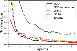
(a) training loss (MNIST)

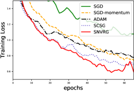
(b) training loss (CIFAR10)

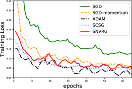
(c) training loss (SVHN)

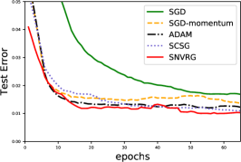
(d) test error (MNIST)

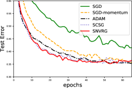
(e) test error (CIFAR10)

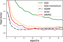
(f) test error (SVHN)

Figure 4: Experimental results on different datasets without learning rate decay. (a) and (d) depict the training loss and test error (top-1 error) v.s. data epochs for training LeNet on MNIST dataset. (b) and (e) depict the training loss and test error v.s. data epochs for training LeNet on CIFAR10 dataset. (c) and (f) depict the training loss and test error v.s. data epochs for training LeNet on SVHN dataset.

Appendix F An Equivalent Version of Algorithm 1

Recall the One-epoch-SNVRG algorithm in Algorithm 1. Here we present an equivalent version of Algorithm 1 using nested loops, which is displayed in Algorithm 4 and is more aligned with the illustration in Figure 2. Note that the notation used in Algorithm 4 is slightly different from that in Algorithm 1 to avoid confusion.

Algorithm 4 One-epoch SNVRG($F,\mathbf{x}_{0},K,M,\{T_{i}\},\{B_{i}\},B$)

1:  Input: Function $F$, starting point $\mathbf{x}_{0}$, loop number $K$, step size parameter $M$, loop parameters $T_{i},i\in[K]$, batch parameters $B_{i},i\in[K]$, base batch $B>0$. Output: $[\mathbf{x}_{\text{out}},\mathbf{x}_{\text{end}}]$

2:  $T\leftarrow\prod_{l=1}^{K}T_{l}$

3:  Uniformly generate index set $I\subset[n]$ without replacement

4:  $\mathbf{g}_{[t_{0}]}^{(0)}\leftarrow\frac{1}{B}\sum_{i\in I}\nabla f_{i_{d}}(\mathbf{x}_{0})$

5:  $\mathbf{x}_{[0]}^{(l)}\leftarrow\mathbf{x}_{0},\quad 0\leq l\leq K$,

6:  for $t_{1}=0,\dots,T_{1}-1$ do

7:     Uniformly generate index set $I\subset[n]$ without replacement, $|I|=B_{1}$

8:     $\mathbf{g}_{[t_{1}]}^{(1)}\leftarrow\frac{1}{B_{1}}\sum_{i\in I}\big{[}\nabla f_{i}(\mathbf{x}_{[t_{1}]}^{(1)})-\nabla f_{i}(\mathbf{x}_{[0]}^{(0)})\big{]}$

9:     $\dots$

10:     for $t_{l}=0,\dots,T_{l}-1$ do

11:        Uniformly generate index set $I\subset[n]$ without replacement, $|I|=B_{l}$

12:        $\mathbf{g}_{[t_{l}]}^{(l)}\leftarrow\frac{1}{B_{l}}\sum_{i\in I}\big{[}\nabla f_{i}(\mathbf{x}_{[t_{l}]}^{(l)})-\nabla f_{i}(\mathbf{x}_{[t_{l-1}]}^{(l-1)})\big{]}$

13:        $\dots$

14:        for $t_{K}=0,\dots,T_{K}-1$ do

15:           Uniformly generate index set $I\subset[n]$ without replacement, $|I|=B_{K}$

16:           $\mathbf{g}_{[t_{K}]}^{(K)}\leftarrow\frac{1}{B_{K}}\sum_{i\in I}\big{[}\nabla f_{i}(\mathbf{x}_{[t_{K}]}^{(K)})-\nabla f_{i}(\mathbf{x}_{[t_{K-1}]}^{(K-1)})\big{]}$

17:           Denote $t=\sum_{j=1}^{K}t_{j}\prod_{l=j+1}^{K}T_{l}$, then let $\mathbf{x}_{t+1}\leftarrow\mathbf{x}_{t}-1/(10M)\cdot\sum_{l=0}^{K}\mathbf{g}_{[t_{l}]}^{(l)}$

18:           $\mathbf{x}_{[t_{K}+1]}^{(K)}\leftarrow\mathbf{x}_{t+1}$

19:        end for

20:        $\dots$

21:        $\mathbf{x}_{[t_{l}+1]}^{(l)}\leftarrow\mathbf{x}_{[T_{l+1}]}^{(l+1)}$

22:     end for

23:     $\dots$

24:     $\mathbf{x}_{[t_{1}+1]}^{(1)}\leftarrow\mathbf{x}_{[T_{2}]}^{(2)}$

25:  end for

26:  $\mathbf{x}_{\text{out}}\leftarrow$ a uniformly random choice from $\{\mathbf{x}_{0},...,\mathbf{x}_{T-1}\}$

27:  return  $[\mathbf{x}_{\text{out}},\mathbf{x}_{T}]$

References

- Agarwal et al. [2017] Naman Agarwal, Zeyuan Allenzhu, Brian Bullins, Elad Hazan, and Tengyu Ma. Finding approximate local minima for nonconvex optimization in linear time. 2017.
- Allen-Zhu [2017a] Zeyuan Allen-Zhu. Katyusha: The first direct acceleration of stochastic gradient methods. In Proceedings of the 49th Annual ACM SIGACT Symposium on Theory of Computing, pages 1200–1205. ACM, 2017a.
- Allen-Zhu [2017b] Zeyuan Allen-Zhu. Natasha 2: Faster non-convex optimization than sgd. arXiv preprint arXiv:1708.08694, 2017b.
- Allen-Zhu [2018] Zeyuan Allen-Zhu. Katyusha x: Simple momentum method for stochastic sum-of-nonconvex optimization. In Proceedings of the 35th International Conference on Machine Learning, volume 80, pages 179–185. PMLR, 10–15 Jul 2018.
- Allen-Zhu and Hazan [2016] Zeyuan Allen-Zhu and Elad Hazan. Variance reduction for faster non-convex optimization. In International Conference on Machine Learning, pages 699–707, 2016.
- Bietti and Mairal [2017] Alberto Bietti and Julien Mairal. Stochastic optimization with variance reduction for infinite datasets with finite sum structure. In Advances in Neural Information Processing Systems, pages 1622–1632, 2017.
- Carmon et al. [2016] Yair Carmon, John C. Duchi, Oliver Hinder, and Aaron Sidford. Accelerated methods for non-convex optimization. 2016.
- Carmon et al. [2017a] Yair Carmon, John C Duchi, Oliver Hinder, and Aaron Sidford. “convex until proven guilty”: Dimension-free acceleration of gradient descent on non-convex functions. In International Conference on Machine Learning, pages 654–663, 2017a.
- Carmon et al. [2017b] Yair Carmon, John C Duchi, Oliver Hinder, and Aaron Sidford. Lower bounds for finding stationary points of non-convex, smooth high-dimensional functions. 2017b.
- Defazio et al. [2014a] Aaron Defazio, Francis Bach, and Simon Lacoste-Julien. Saga: A fast incremental gradient method with support for non-strongly convex composite objectives. In Advances in Neural Information Processing Systems, pages 1646–1654, 2014a.
- Defazio et al. [2014b] Aaron Defazio, Justin Domke, et al. Finito: A faster, permutable incremental gradient method for big data problems. In International Conference on Machine Learning, pages 1125–1133, 2014b.
- Fang et al. [2018] Cong Fang, Chris Junchi Li, Zhouchen Lin, and Tong Zhang. Spider: Near-optimal non-convex optimization via stochastic path-integrated differential estimator. In Advances in Neural Information Processing Systems, pages 686–696, 2018.
- Garber and Hazan [2015] Dan Garber and Elad Hazan. Fast and simple pca via convex optimization. arXiv preprint arXiv:1509.05647, 2015.
- Ghadimi and Lan [2012] Saeed Ghadimi and Guanghui Lan. Optimal stochastic approximation algorithms for strongly convex stochastic composite optimization i: A generic algorithmic framework. SIAM Journal on Optimization, 22(4):1469–1492, 2012.
- Ghadimi and Lan [2016] Saeed Ghadimi and Guanghui Lan. Accelerated gradient methods for nonconvex nonlinear and stochastic programming. Mathematical Programming, 156(1-2):59–99, 2016.
- Harikandeh et al. [2015] Reza Harikandeh, Mohamed Osama Ahmed, Alim Virani, Mark Schmidt, Jakub Konečnỳ, and Scott Sallinen. Stopwasting my gradients: Practical svrg. In Advances in Neural Information Processing Systems, pages 2251–2259, 2015.
- Hillar and Lim [2013] Christopher J Hillar and Lek-Heng Lim. Most tensor problems are np-hard. Journal of the ACM (JACM), 60(6):45, 2013.
- Hu et al. [2009] Chonghai Hu, Weike Pan, and James T Kwok. Accelerated gradient methods for stochastic optimization and online learning. In Advances in Neural Information Processing Systems, pages 781–789, 2009.
- Johnson and Zhang [2013] Rie Johnson and Tong Zhang. Accelerating stochastic gradient descent using predictive variance reduction. In Advances in neural information processing systems, pages 315–323, 2013.
- Karimi et al. [2016] Hamed Karimi, Julie Nutini, and Mark Schmidt. Linear convergence of gradient and proximal-gradient methods under the polyak-łojasiewicz condition. In Joint European Conference on Machine Learning and Knowledge Discovery in Databases, pages 795–811. Springer, 2016.
- Kingma and Ba [2014] Diederik P Kingma and Jimmy Ba. Adam: A method for stochastic optimization. arXiv preprint arXiv:1412.6980, 2014.
- Krizhevsky [2009] Alex Krizhevsky. Learning multiple layers of features from tiny images. 2009.
- Lan [2012] Guanghui Lan. An optimal method for stochastic composite optimization. Mathematical Programming, 133(1):365–397, 2012.
- Lan and Zhou [2017] Guanghui Lan and Yi Zhou. An optimal randomized incremental gradient method. Mathematical programming, pages 1–49, 2017.
- LeCun et al. [1998] Yann LeCun, Léon Bottou, Yoshua Bengio, and Patrick Haffner. Gradient-based learning applied to document recognition. Proceedings of the IEEE, 86(11):2278–2324, 1998.
- Lei et al. [2017] Lihua Lei, Cheng Ju, Jianbo Chen, and Michael I Jordan. Non-convex finite-sum optimization via scsg methods. In Advances in Neural Information Processing Systems, pages 2345–2355, 2017.
- Li and Lin [2015] Huan Li and Zhouchen Lin. Accelerated proximal gradient methods for nonconvex programming. In Advances in neural information processing systems, pages 379–387, 2015.
- Li et al. [2017] Qunwei Li, Yi Zhou, Yingbin Liang, and Pramod K Varshney. Convergence analysis of proximal gradient with momentum for nonconvex optimization. arXiv preprint arXiv:1705.04925, 2017.
- Lin et al. [2015] Hongzhou Lin, Julien Mairal, and Zaid Harchaoui. A universal catalyst for first-order optimization. In Advances in Neural Information Processing Systems, pages 3384–3392, 2015.
- Mairal [2015] Julien Mairal. Incremental majorization-minimization optimization with application to large-scale machine learning. SIAM Journal on Optimization, 25(2):829–855, 2015.
- Nesterov [2005] Yu Nesterov. Smooth minimization of non-smooth functions. Mathematical programming, 103(1):127–152, 2005.
- Nesterov [2014] Yurii Nesterov. Introductory Lectures on Convex Optimization. Kluwer Academic Publishers, 2014.
- [33] Yuval Netzer, Tao Wang, Adam Coates, Alessandro Bissacco, Bo Wu, and Andrew Y Ng. Reading digits in natural images with unsupervised feature learning.
- Nguyen et al. [2017a] Lam M Nguyen, Jie Liu, Katya Scheinberg, and Martin Takáč. Sarah: A novel method for machine learning problems using stochastic recursive gradient. In Proceedings of the 34th International Conference on Machine Learning-Volume 70, pages 2613–2621. JMLR. org, 2017a.
- Nguyen et al. [2017b] Lam M Nguyen, Jie Liu, Katya Scheinberg, and Martin Takáč. Stochastic recursive gradient algorithm for nonconvex optimization. arXiv preprint arXiv:1705.07261, 2017b.
- Paquette et al. [2017] Courtney Paquette, Hongzhou Lin, Dmitriy Drusvyatskiy, Julien Mairal, and Zaid Harchaoui. Catalyst acceleration for gradient-based non-convex optimization. arXiv preprint arXiv:1703.10993, 2017.
- Polyak [1964] Boris T Polyak. Some methods of speeding up the convergence of iteration methods. USSR Computational Mathematics and Mathematical Physics, 4(5):1–17, 1964.
- Polyak [1963] Boris Teodorovich Polyak. Gradient methods for minimizing functionals. Zhurnal Vychislitel’noi Matematiki i Matematicheskoi Fiziki, 3(4):643–653, 1963.
- Qian [1999] Ning Qian. On the momentum term in gradient descent learning algorithms. Neural networks, 12(1):145–151, 1999.
- Reddi et al. [2016a] Sashank J. Reddi, Ahmed Hefny, Suvrit Sra, Barnabas Poczos, and Alex Smola. Stochastic variance reduction for nonconvex optimization. pages 314–323, 2016a.
- Reddi et al. [2016b] Sashank J Reddi, Suvrit Sra, Barnabás Póczos, and Alex Smola. Fast incremental method for smooth nonconvex optimization. In Decision and Control (CDC), 2016 IEEE 55th Conference on, pages 1971–1977. IEEE, 2016b.
- Reddi et al. [2016c] Sashank J Reddi, Suvrit Sra, Barnabas Poczos, and Alexander J Smola. Proximal stochastic methods for nonsmooth nonconvex finite-sum optimization. In Advances in Neural Information Processing Systems, pages 1145–1153, 2016c.
- Roux et al. [2012] Nicolas L Roux, Mark Schmidt, and Francis R Bach. A stochastic gradient method with an exponential convergence _rate for finite training sets. In Advances in Neural Information Processing Systems, pages 2663–2671, 2012.
- Schölkopf and Smola [2002] Bernhard Schölkopf and Alexander J Smola. Learning with kernels: support vector machines, regularization, optimization, and beyond. MIT press, 2002.
- Shalev-Shwartz [2015] Shai Shalev-Shwartz. Sdca without duality. arXiv preprint arXiv:1502.06177, 2015.
- Shalev-Shwartz [2016] Shai Shalev-Shwartz. Sdca without duality, regularization, and individual convexity. In International Conference on Machine Learning, pages 747–754, 2016.
- Shalev-Shwartz and Zhang [2013] Shai Shalev-Shwartz and Tong Zhang. Stochastic dual coordinate ascent methods for regularized loss minimization. Journal of Machine Learning Research, 14(Feb):567–599, 2013.
- Xiao and Zhang [2014] Lin Xiao and Tong Zhang. A proximal stochastic gradient method with progressive variance reduction. SIAM Journal on Optimization, 24(4):2057–2075, 2014.