A Gap in the Lower Main Sequence Revealed by Gaia Data Release 2

Abstract

We present the discovery of a gap near $M_{G}\approx$10 in the main sequence on the Hertzsprung-Russell Diagram (HRD) based on measurements presented in Gaia Data Release 2 (DR2). Using an observational form of the HRD with $M_{G}$ representing luminosity and $G_{BP}-G_{RP}$ representing temperature, the gap presents a diagonal feature that dips toward lower luminosities at redder colors. The gap is seen in samples extracted from DR2 with various distances, and is not unique to the Gaia photometry — it also appears when using near-IR photometry ($J-K_{s}$ vs $M_{K_{s}}$). The gap is very narrow ($\sim$0.05 mag) and is near the luminosity-temperature regime where M dwarf stars transition from partially to fully convective, i.e., near spectral type M3.0V. This gap provides a new feature in the H-R Diagram that hints at an underlying astrophysical cause and we propose that it is linked to the onset of full convection in M dwarfs.

1 Introduction

The Hertzsprung-Russell Diagram (HRD) provides the most fundamental map in stellar astronomy, relating key information about stars of many types. The HRD typically relates a star’s luminosity and temperature, but we can also derive related quantities that change a star’s precise location on the HRD, including its size, metallicity, and of course, evolutionary state. To place a star on an HRD, astronomers need an essential measurement of its distance, most reliably measured via a trigonometric parallax. The practice of measuring parallaxes started with F. Bessel, who determined the parallax for 61 Cygni in 1838 (Bessel, 1838). Since then, astronomers have made most parallax measurements from the ground by pointing telescopes at stars one at a time. Results of ground-based astrometry programs as of 1995 were summarized in The General Catalogue of Trigonometric Stellar Parallaxes (also known as the “Yale Parallax Catalog”, or YPC) (van Altena et al., 1995), a valuable compendium to which more recent programs have added.

In 1989, the European Space Agency (ESA) launched the Hipparcos mission to measure parallaxes systematically for most stars brighter than $V\approx$9, and improved the precision on parallaxes to a few milli-arcseconds in most cases (Perryman et al., 1997). Although three-dimensional space was well-mapped by Hipparcos for bright stars, distances for relatively few of the ubiquitous red dwarfs were measured. Although the YPC included parallaxes for several thousand red dwarfs, several ground based astrometry programs continued to do the heavy lifting of measuring distances star-by-star (see, for example the 38 references in Henry et al. (2018), Table 4). In one case, a full-sky survey that provided thousands of parallaxes with a particular focus on stars within 25 pc has been carried out by the USNO (Finch & Zacharias, 2016; Finch et al., 2018). Even so, most red dwarfs within 100 pc did not have distance measurements.

In 2013, the launch of the Gaia mission initiated a new era of astrometry measurements for virtually all types of stars on the HRD (Gaia Collaboration et al., 2016). In April 2018, Gaia Data Release 2 (DR2) provided unprecedented sub-milliarcsecond parallax precision for over a billion stars (Gaia Collaboration et al., 2018a) that can be utilized to study the precise locations of individual stars on the HRD as well as populations of stars. The wealth of precise, all-sky data yields an HRD that reveals never-before-seen features that were previously impossible to identify. For example, in Gaia Collaboration et al. (2018b) and Kilic et al. (2018), it was shown that (1) there are two main sequences in the HRD for nearby stars caused by a metallicity difference of about 1 dex, and (2) the distribution of nearby white dwarfs on the HRD shows multiple sequences due to different atmosphere compositions and mass distributions.

In this work, we present a new feature of the main sequence – a gap at mid-M dwarfs.

2 The Gap

A gap, shown in Figure 1, in the distribution of red dwarfs is discovered using stars within 100 pc in DR2. Data were retrieved from the Gaia archive using an ADQL script of 
SELECT * FROM gaiadr2.gaia_source WHERE parallax >=10, resulting in a sample of 700,055 extracted sources. Data cleaning was accomplished by using the three-step cuts discussed in Lindegren et al. (2018), primarily to remove low quality sources, many of which fell between main sequence and white dwarfs on the HRD; a total of 242,582 sources remained. A portion of the HRD focused on M dwarfs is shown in Figure 1, where a low density gap cuts through the main sequence at $M_{G}\approx$10.

Figure 1: A portion of the observational HRD for stars within 100 pc in the Gaia DR2 dataset, using $M_{G}$ and $G_{BP}-G_{RP}$. A thin, low density, gap is seen cutting through the main sequence. Two dashed lines ($M_{G}=$ 9 and 11) represent a region selected for further discussion, and plotted in Figure 2.

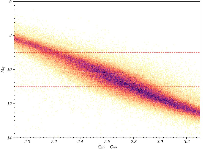
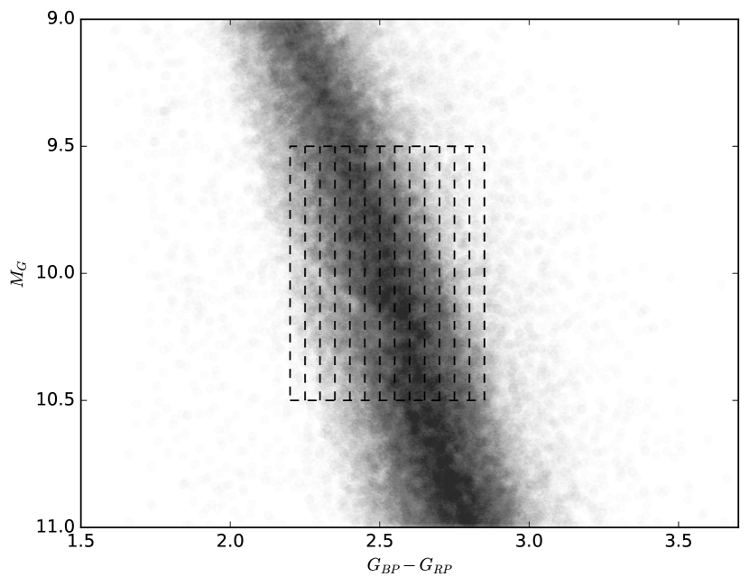
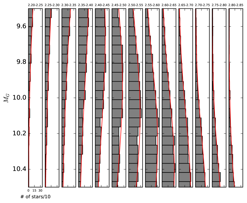
To further highlight and quantify the stellar population near this gap, a zoomed region between the two dashed lines in Figure 1 has been sliced into several strips as shown in the left panel of Figure 2. Histograms of star counts in each strip are illustrated in the right panel and show that the gap progresses from $M_{G}\sim$10.09 in the $G_{BP}-G_{RP}$= 2.35–2.40 bin to $\sim$10.24 in the 2.55–2.60 bin. Comparison to Gaussian models of star distributions along the $M_{G}$ axis (shown in red in the right panel of Figure 2) indicates that the decrements of stars in the gap regions are $\sim$24% and 14% less than the Gaussian curves, respectively, in these two bins. This also shows the gap is very narrow, with a width of only about 0.05 mag. Furthermore, it is more pronounced at blue colors than at red. The largest decrement is 28% in the 2.40–2.45 bin. The details of these decrements in each bin are summarized in Table 1.

Table 1: Percentage decrement along the gap for different samples

		0-100pc	100-130pc	120-130pc
		70,700	81,600	31,610
$G_{BP}-G_{RP}$ bin	$M_{G}$ with largest decrement	percentage decrement	percentage decrement	percentage decrement
2.30-2.35	10.04	19(73/90.2)	11(90/100.6)	25(29/38.4)
2.35-2.40	10.09	24(95/125.3)	12(125/142.2)	21(42/52.9)
2.40-2.45	10.14	28(122/168.8)	19(152/188.6)	24(53/69.6)
2.45-2.50	10.19	23(173/225.5)	30(178/254.5)	28(70/97.4)
2.50-2.60	10.24	22(211/271.4)	16(256/302.9)	10(107/118.9)
2.55-2.60	10.24	14(264/307.7)	16(290/344.2)	18(108/131.5)
2.60-2.65	10.29	7(275/297.0)	11(303/340.1)	12(121/137.9)
2.65-2.70	10.34	12(236/296.3)	12(271/307.4)	11(107/120.5)

Note. — The total numbers of stars in each sample are given in the second row, and these stars have $M_{G}$ between 9.0 and 11.0. Two numbers in the parentheses indicate the actual start counts (integer) and fitted Gaussian counts (real number) in each bin.

Figure 2: (left) Sliced strips of the main sequence near the gap are shown, with vertical cuts in $G_{BP}-G_{RP}$ color. (right) Distributions of the number of stars in each $G_{BP}-G_{RP}$ strip are shown, with Gaussian fits outlined in red. Each vertical strip is 0.05 mag wide in color, and the histogram bin sizes are 0.051 mag in $M_{G}$ to optimize the gap’s effect.

3 The Gap in Different Colors and More Distant Samples

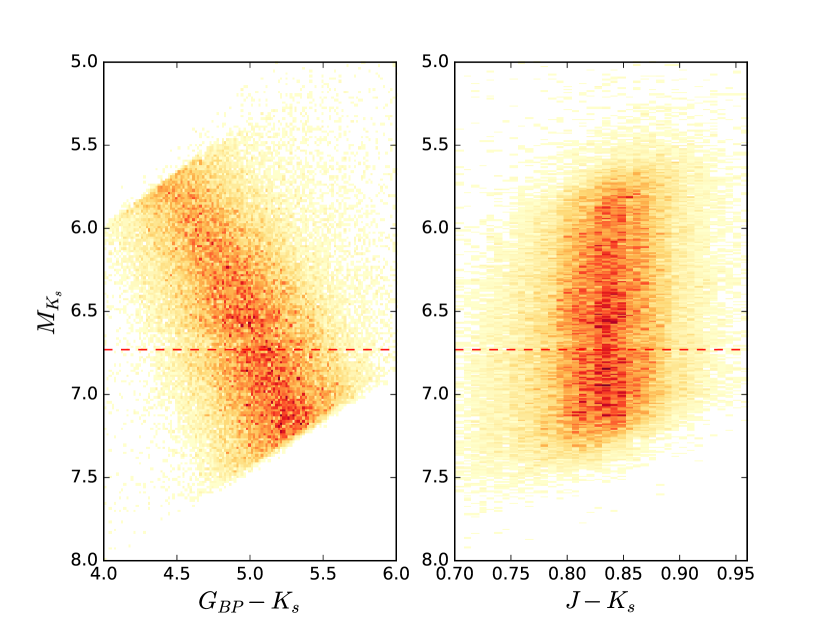
An important consideration is whether or not the gap persists in colors other than $G_{BP}-G_{RP}$. To investigate, 70,700 stars between the two dashed lines in Figure 1 were cross-matched against the 2MASS catalog. Because many of these nearby red dwarfs have high proper motions, the J2015.5 coordinates in DR2 were adjusted to J2000.0 using the DR2 proper motions so that their coordinates would be close to their positions in 2MASS images, which were taken from 1998–2001. A 5″ search radius was then used to find matches of DR2 sources to 2MASS sources. Figure 3 shows two different HRDs, $G_{BP}-K_{s}$ vs $M_{K_{s}}$ and $J-K_{s}$ vs. $M_{K_{s}}$, that illustrate the results. Somewhat surprisingly, the gap is evident in these two observational HRDs as well. Thus, the gap is not unique to the Gaia photometry, and is not caused by specific stellar spectroscopic features in the optical or near-infrared bands alone.

Figure 3: Two observational HRDs are shown using $M_{K_{s}}$ for luminosity and $G_{BP}-K_{s}$ and $J-K_{s}$ for temperature. The gap is seen in both plots, indicating that the gap persists at both optical and infrared wavelengths. Red dashed lines mark the $M_{K_{s}}=$6.73 value that corresponds to stars with mass 0.35$M_{\odot}$ based on the mass-luminosity relation of Benedict et al. (2016). The gap is seen in both panels slightly above the dashed lines.

In order to test the persistence of the gap, we extracted two other samples from DR2 using stars in the 100–130 pc and 120–130 pc shells. After applying the three-step cuts in Lindegren et al. (2018), 81,600 and 31,610 stars are left, respectively. The 100–130 pc shell is selected to have a similar number of stars and volume as stars in 0–100 pc. The other 120–130 pc shell contains about half the number of stars in 0–100pc and a totally different set of stars. HRDs for the three samples are presented side-by-side in Figure 4.

We see the same gap at the exact same location in all three HRD. The 120–130 pc sample size is only $\sim$45% the size of the sample in the 0–100 pc range, so the gap is not as obvious. Although the 100–130 pc sample size is the largest, its gap is not the sharpest because stars in 100–130 pc range have relatively smaller parallax to parallax error ratios. Hence, parallax errors become more significant at larger distances, thereby shifting stars slightly on the HRD, with a consequent blurring of the distribution near and in the gap. We note that samples of the nearest stars, such as those within 25 pc in DR2, do not show the gap because there are only $\sim$4000 points spanning the entire main sequence.

Figure 4: Three HRDs of different samples, 0–100, 100–130 and 120–130 pc from Gaia DR2 are shown from left to right. The total numbers of stars used in each sample are given in Table 1.

4 Discussion

The detection of a new feature in the HRD implies a previously unknown characteristic of stars that may be linked to fundamental astrophysics. This leads to a number of questions that need to be considered.

Is the gap due to a bias in Gaia data? According to Gaia Collaboration et al. (2018a), (1) “a fraction of the bright stars at $G<$7 is still missing with no stars brighter than $G=$1.7 mag appearing in DR2” and (2) 17% of stars with proper motions greater than 0$\farcs$6 yr^-1 could still be missing. Thus, there appear to be no biases that would omit stars near the gap in the DR2 dataset.

Is this gap caused by the presence of multiple main sequences? The double main sequence bands shown in Figure 21 of Gaia Collaboration et al. (2018b) are almost parallel and almost evenly spread apart. Globular clusters like NGC6397 (Milone et al., 2012) and $\omega$ Centauri (Bedin et al., 2004) also have double main sequences and their dividing lines are similar to the one seen in Gaia Collaboration et al. (2018b). The gap we outline here for nearby stars has a very different slope, so is not consistent with gaps resulting from multiple main sequence populations.

Can the gap be reproduced for stars in other parts of the Galaxy? The ideal laboratories in which to search for the gap are open or globular clusters, because such stellar groups comprise relatively clean samples given the similar ages and metallicities of members. Unfortunately, no open clusters are known to have the tens of thousands (at least) of stars needed to define the gap. The nearest globular cluster, NGC 6397, has been observed by Gaia, but cannot be used to confirm the gap because the faintest stars observed are $\sim$1 magnitude bluer in $G_{BP}-G_{RP}$ color than the gap shown in Figure 1. Richer et al. (2008) presented a color-magnitude diagram for NGC 6397 from a deep survey using HST/ACS that reached down the main sequence to late-type M dwarfs (see their Figure 6). Unfortunately, because of the low number of stars around the gap region, no reliable test of the gap can be done.

Why has this gap not been seen before? Before the DR2 dataset, the available number of parallaxes for M dwarfs were both (1) limited in number, and (2) had larger errors. Because the gap is narrow and subtle, these two attributes of the available parallax sets precluded identifying the gap — a much larger set of high-precision parallaxes is needed.

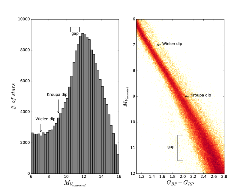
Is the gap related to the “Wielen dip” or “Kroupa dip”? The Wielen dip was first reported in Wielen et al. (1983) while studying the luminosity function of nearby stars using the 1969 version of the Catalogue of Nearby Stars (Gliese, 1969). The dip occurs at $M_{V}\approx$7, corresponding to mid-K type dwarfs, i.e., at much earlier types than the gap described here near M3.0V type (Figure 6). Kroupa et al. (1990) and Kroupa (2002) proposed that this depression/plateau in the luminosity function is due to H^- opacity becoming increasingly important in the atmospheres of K dwarfs, reducing their luminosities to create the (slight) dip marked in Figure 5.

The other so-called “Kroupa dip” at $M_{V}\approx$9 can be seen in the stellar luminosity function of field stars in Kroupa et al. (1990) and its location is marked in Figure 5. Elsanhoury et al. (2011) studied both dips using several open clusters, and showed “both dips may not be strongly visible” in the luminosity function of clusters. Even though both features are called “dips”, they are almost invisible in the HRD plot of Figure 5 compared to this DR2 gap.

The gap discussed here spreads from $M_{Vconverted}$$\sim$10.5–11.5 and is dependent on color, so is not clearly represented in the histogram of Figure 5. Regardless, it is clear that both Wielen and Kroupa dips are much bluer than the gap we see in DR2 data.

Figure 5: (Left) The stellar luminosity function based on Gaia DR2 data is shown. The Johnson $V$ magnitudes have been converted using the transformation discussed in Appendix A. The “Wielen dip” and “Kroupa dip” are roughly marked at $M_{V}\approx 7$ and $9$, respectively. The gap discussed here is outlined with a bracket shown at $M_{V}$=10.5–11.5. (Right) The different dips and the DR2 gap are marked on the HRD, and this DR2 gap is very obvious.

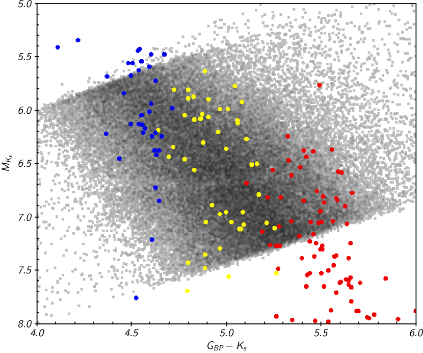
Is the gap related to the onset of full convection in $\sim$M3.0V stars? As shown in Figure 6, the gap maps onto spectral type $\sim$M3.0V, where blue, yellow, and red points represent single stars within 25 pc with spectral types of M2.0V, M3.0V, and M4.0V, respectively. This is the location on the main sequence where interior structure models show a transition from partially to fully convective stars (Limber, 1958; Hayashi & Nakano, 1963; Dorman et al., 1989; Chabrier & Baraffe, 1997) at $\sim$0.35$M_{\odot}$. Recent theoretical stellar models (Marigo et al., 2017; Baraffe et al., 2015; Dotter et al., 2008) are generally smooth from high to low masses, including through the M dwarfs, with no abrupt transitions.

Figure 6: An observational HRD using $G_{BP}-K_{s}$ and $M_{K_{s}}$ to separate different spectral types of stars. Blue, yellow and red circles represent known single stars within 25 pc with spectral types of M2.0V, M3.0V, and M4.0V, respectively.

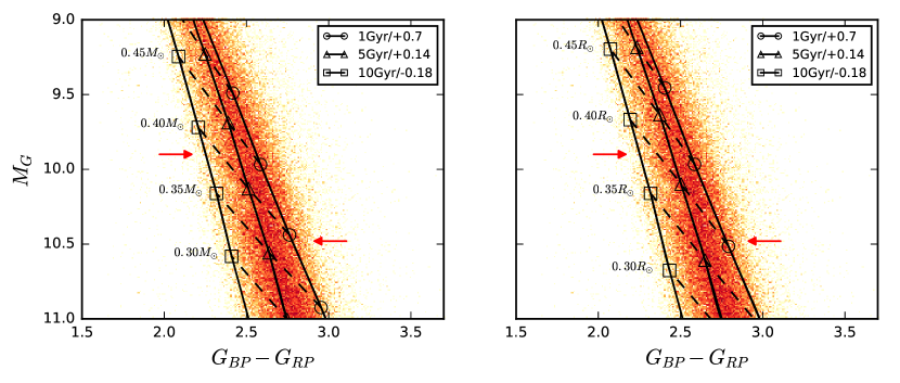
Model isochrones can help us estimate the mass and radii associated with the gap, although we caution that stellar models still have difficulties in matching the color-magnitude diagrams of low mass stars in clusters (Chen et al., 2014). Two selected models to be compared to the Gaia data are PARSEC (Marigo et al., 2017) and YaPSI (Spada et al., 2017).

We plot three different isochrones from PARSEC in Figure 7. Most isochrone parameters are default values at this website, other than ages and metallicities. Three isochrones shown are 1 Gyr/[M/H]=+0.7, 5 Gyrs/[M/H]=+0.14 and 10 Gyrs/[M/H]=$-$0.18. We can see that the gap intercepts the 0.4$M_{\odot}$ equal-mass and 0.4$R_{\odot}$ equal-radius lines. Although the gap’s slope is somewhat different than these two lines, we expect the slope of the gap is caused by varying metallicities and ages of these nearby stars at a given mass or radius. As Figure 1 shows, this gap is more prominent in the blue, implying that low metallicity stars tend to deepen this gap.

Figure 7: Three different isochrones (solid lines) from PARSEC are shown on the HRD. Circles, triangles and square boxes represent three different isochrones given in the legends. Dashed lines represent equal masses (left figure) and radii (right figure) on all three isochrones. Because these two figures are crowded, identifying this gap becomes difficult. Two arrows mark the gap location and the gap feature appears to have a shallower slope than either the equal-mass line at 0.4$M_{\odot}$ or equal-radius line at 0.4$R_{\odot}$.

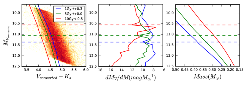
We also retrieved three different YaPSI isochrones with $VRIJHK$ colors based on Worthey & Lee (2011) from their website . The three different isochrones are shown in the left plot of Figure 8 along with the Gaia data. Because YaPSI models have a much finer grid step size (0.01M_⊙) than those in PARSEC (0.05$M_{\odot}$), a discontinuity in the slope of the isochrone is revealed near the location of the gap. As Spada et al. (2017) pointed out, the kink close to 0.35M_⊙ in the mass-luminosity relation occurs because of the transition from fully convective to solar-like interior structure. These kinks are where the slopes of mass-luminosity relations change and are marked as three dashed lines in Figure 8. The transitions are approximately at 0.38, 0.37, and 0.33M_⊙, respectively for [Fe/H]=+0.3, 0.0 and $-$0.5. Discontinuities in the slopes of the isochrones are associated with a drop in the number densities in the gap region. We expect that the increment in stellar number $N$ varies as

$${{dN}\over{dM_{V}}}={{dN}\over{dM}}/{{dM_{V}}\over{dM}}$$

where ${{dN}\over{dM}}$ is the continuous stellar mass function and ${{dM_{V}}\over{dM}}$ is the predicted change in absolute magnitude with stellar mass. The right panel of Figure 8 shows the discontinuities in the $(M,M_{V})$ plane, while the central panel shows the absolute magnitude as a function of the local numerical derivative ${{dM_{V}}\over{dM}}$. We see that the predicted magnitudes where the model ${{dM_{V}}\over{dM}}$ attains a local minimum correspond to those magnitudes with fewer stars, i.e., where the gaps are located on the HRD. We note that the three YaPSI isochrones are significantly shifted to the blue relative to the Gaia data, unlike the PARSEC models shown in Figure 7.

Figure 8: Three different isochrones (solid lines) from YaPSI are plotted against the Gaia data on the HRD. Blue, green and red lines represent three different isochrones, 1Gyr/[Fe/H]=+0.3/X=0.717/Z=0.03, 5Gyr/[Fe/H]=+0.0/X=0.733/Z=0.016 and 10Gyr/[Fe/H]=-0.5/X=0.744/Z=0.005, respectively, and all isochrones have Y=0.25. The Gaia BP magnitudes are converted to $V$ using the relation discussed in Appendix A. We note that these isochrones do not contain 2MASS $K_{s}$ magnitudes, but we believe the difference between $K$ and $K_{s}$ is small. The middle plot is the slope of the mass-luminosity relations of these three metallicities shown on the right. Three colored dashed lines mark where the MLR slopes have local minima at $M_{V}=$11.36, 11.06 and 10.56.

Observationally, the empirical mass-luminosity relation (Benedict et al., 2016), temperature-radius relation (Ribas, 2006; Boyajian et al., 2012), and large scale magnetic topology studies of M dwarfs (Morin et al., 2010) also show relatively smooth transitions based on small samples. The narrow gap implies a “sudden” transition from one state to another, which happens to fall near the mass where stars are modelled to become fully convective. This presents a conundrum: we typically refer to stars beginning to be fully convective at a given temperature corresponding to spectral type $\sim$M3.0V, implying a vertical gap in the HRD, but we observe that the gap is roughly horizontal in $M_{G}$, $M_{V}$ and $M_{Ks}$.

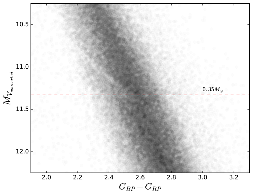
Using the mass-luminosity relation of Benedict et al. (2016), 0.35$M_{\odot}$ corresponds to $M_{K_{s}}$ = 6.73 and $M_{V}$ = 11.33. These values are marked with dashed lines in Figure 3 for $M_{K_{s}}$ and Figure 9 for $M_{V}$, and in both cases fall near the gaps. It is important to point out that the 0.35$M_{\odot}$ value for the transition to fully convective stars is approximate, and the Benedict et al. (2016) sample used to estimate the absolute magnitudes for 0.35$M_{\odot}$ stars is a heterogeneous mix of stars in the solar neighborhood with various metallicities and magnetic properties.

All the evidence shown above is quite compelling — it is probable that gap and the transition to fully convective stars are linked. More importantly, no other region of the main-sequence has a similar gap like this. The result implies that stars above the gap may prove to be mostly convective with a thin radiative layer and more massive, while those below are fully convective less massive and smaller.

Figure 9: An observational HRD using $G_{BP}-G_{RP}$ and $M_{V_{converted}}$ is shown. The red dashed line that intersects the gap marks the $M_{V_{s}}=$11.33 value that corresponds to stars with mass 0.35$M_{\odot}$ based on the mass-luminosity relation of Benedict et al. (2016) from nearby stars with various metallicities.

5 Future Study of the Gap

This new feature on the HRD shows the power of high precision astrometry and challenges how we understand all regions in the fundamental map of stellar luminosities and temperatures. It appears that there is a small slice of the HRD that is less populated, at least relative to surrounding regions in luminosity and temperature. Based on the evidence presented here, the observed drop in stellar numbers in the gaps is probably related to a subtle change in structure (decrease in radius) that occurs at the transition between partially and fully convective stars.

We suggest the following studies be undertaken to further understand this new feature on the HRD. (1) Examine the stars currently falling in the gap to evaluate contamination from unresolved multiples, thereby providing a better assessment of the true depth of the decrement in population. (2) Measure accurate dynamical masses, radii and metallicities for stars on both sides of the gap, as well as those remaining in the gap, to understand the characteristics across this region of the HRD. (3) Determine the rotational periods for stars in and around the gap to see if there are any trends. (4) Evaluate the photometric variability as a proxy for investigating the effects of magnetism, or measure magnetic topology of stars in this region of the HRD to determine if there are any variations that provide clues as to the cause of the gap.

Appendix A Converting Gaia ($G_{BP}$ and $G_{RP}$) to Johnson–Kron–Cousin ($V$ and $I$)

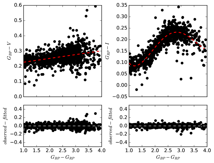
Evans et al. (2018) provides a transformation equation to convert Gaia $G$ magnitudes to Johnson $V$. Because the $G$ bandpass is much wider than $V$ and includes significantly more red flux, we provide transformations from $G_{BP}$ to Johnson $V$ and $G_{RP}$ to Kron-Cousin $I$. We use ground-based photometry measurements for 1,223 single stars with $V$ for the $G_{BP}$–$V$ relation and 984 single stars with $I$ for the $G_{RP}$–I relation. The stars have spectral types K0V to M6V and are within 25 pc. The total numbers of stars used for these two relations are different because some stars do not have both $V$ and $I$ magnitudes. The two relations are shown in Figure 10, and transformation coefficients are given in Table 2.

Figure 10: The top left panel represents a relation between $G_{BP}-G_{RP}$ and $G_{BP}-V$, where the lower left panel shows the differences between the observed and fitted values. The red dashed line in the top figure represents the best fit line, and a white dashed line in the bottom figure represents zero point. The right two figures are similar, but for the $G_{BP}-G_{RP}$ and $G_{RP}-I$ relation.

Table 2: Coefficients of the polynomials used to convert photometric colors

conv	$c_{0}$	$c_{1}$	$c_{2}$	$c_{3}$	$c_{4}$	$\sigma$
$G_{BP}-V$	0.20220	0.02489	$\cdots$	$\cdots$	$\cdots$	0.04035
$G_{RP}-I$	0.75319	-1.41105	1.00136	-0.27106	0.02489	0.02770

Note. — These relations are valid for 1.0$\leq$$G_{BP}-G_{RP}$$\leq$4.0. The transformations have the following format where color=$G_{BP}-G_{RP}$: $conv=c_{0}+c_{1}\times color+c_{2}\times color^{2}+c_{3}\times color^{3}+c_{4}\times color^{4}$. The seventh column, $\sigma$, represents standard deviations of differences between observed and fitted values shown in the bottom two panels of Figure 10.

Appendix B Plotting programs used to show this gap

Because this gap is not obvious on the HRD, we use two different plotting programs and settings to show this gap and they are summarized below.

Fig 1: TOPCAT/density plot
Fig 2 and 9: Python Matplotlib/scatter plot with alpha=0.01
Fig 3: Python Matplotlib/2D histogram with a regular color scale
Fig 4, 5, 7 and 8: Python Matplotlib/2D histogram with a logarithmic color scale
Fig 6: TOPCAT/scatter plot

References

- Baraffe et al. (2015) Baraffe, I., Homeier, D., Allard, F., & Chabrier, G. 2015, A&A, 577, A42
- Bedin et al. (2004) Bedin, L. R., Piotto, G., Anderson, J., et al. 2004, ApJ, 605, L125
- Benedict et al. (2016) Benedict, G. F., Henry, T. J., Franz, O. G., et al. 2016, AJ, 152, 141
- Bessel (1838) Bessel, F. W. 1838, MNRAS, 4, 152
- Boyajian et al. (2012) Boyajian, T. S., von Braun, K., van Belle, G., et al. 2012, ApJ, 757, 112
- Chabrier & Baraffe (1997) Chabrier, G., & Baraffe, I. 1997, A&A, 327, 1039
- Chen et al. (2014) Chen, Y., Girardi, L., Bressan, A., et al. 2014, MNRAS, 444, 2525
- Dorman et al. (1989) Dorman, B., Nelson, L. A., & Chau, W. Y. 1989, ApJ, 342, 1003
- Dotter et al. (2008) Dotter, A., Chaboyer, B., Jevremović, D., et al. 2008, ApJS, 178, 89-101
- Elsanhoury et al. (2011) Elsanhoury, W. H., Hamdy, M. A., Nouh, M. I., Saad, A. S., & Saad, S. M. 2011, ISRN Astronomy and Astrophysics, 2011, 127030
- Evans et al. (2018) Evans, D. W., Riello, M., De Angeli, F., et al. 2018, arXiv:1804.09368
- Finch & Zacharias (2016) Finch, C. T., & Zacharias, N. 2016, AJ, 151, 160
- Finch et al. (2018) Finch, C. T., Zacharias, N., & Jao, W.-C. 2018, AJ, 155, 176
- Gaia Collaboration et al. (2016) Gaia Collaboration, Prusti, T., de Bruijne, J. H. J., et al. 2016, A&A, 595, A1
- Gaia Collaboration et al. (2018a) Gaia Collaboration, Brown, A. G. A., Vallenari, A., et al. 2018a, arXiv:1804.09365
- Gaia Collaboration et al. (2018b) Gaia Collaboration, Babusiaux, C., van Leeuwen, F., et al. 2018b, arXiv:1804.09378
- Gliese (1969) Gliese, W. 1969, Veroeffentlichungen des Astronomischen Rechen-Instituts Heidelberg, 22, 1
- Hayashi & Nakano (1963) Hayashi, C., & Nakano, T. 1963, Progress of Theoretical Physics, 30, 460
- Henry et al. (2018) Henry, T. J., Jao, W.-C., Winters, J. G., et al. 2018, arXiv:1804.07377
- Hertzsprung (1922) Hertzsprung, E. 1922, Bull. Astron. Inst. Netherlands, 1, 21
- Kilic et al. (2018) Kilic, M., Hambly, N. C., Bergeron, P., Genest-Beaulieu, C., & Rowell, N. 2018, arXiv:1805.01227
- Kroupa et al. (1990) Kroupa, P., Tout, C. A., & Gilmore, G. 1990, MNRAS, 244, 76
- Kroupa (2002) Kroupa, P. 2002, Science, 295, 82
- Lee (1991) Lee, S.-G. 1991, Proceedings of the Astronomical Society of Australia, 9, 209
- Limber (1958) Limber, D. N. 1958, ApJ, 127, 387
- Lindegren et al. (2018) Lindegren, L., Hernandez, J., Bombrun, A., et al. 2018, arXiv:1804.09366
- Marigo et al. (2017) Marigo, P., Girardi, L., Bressan, A., et al. 2017, ApJ, 835, 77
- Milone et al. (2012) Milone, A. P., Marino, A. F., Piotto, G., et al. 2012, ApJ, 745, 27
- Morin et al. (2010) Morin, J., Donati, J.-F., Petit, P., et al. 2010, MNRAS, 407, 2269
- Ribas (2006) Ribas, I. 2006, Ap&SS, 304, 89
- Richer et al. (2008) Richer, H. B., Dotter, A., Hurley, J., et al. 2008, AJ, 135, 2141
- Perryman et al. (1997) Perryman, M. A. C., Lindegren, L., Kovalevsky, J., et al. 1997, A&A, 323, L49
- Spada et al. (2017) Spada, F., Demarque, P., Kim, Y.-C., Boyajian, T. S., & Brewer, J. M. 2017, ApJ, 838, 161
- Taylor (2005) Taylor, M. B. 2005, Astronomical Data Analysis Software and Systems XIV, 347, 29
- van Altena et al. (1995) van Altena, W. F., Lee, J. T., & Hoffleit, D. 1995, The General Catalogue of Trigonometric Stellar Parallaxes (4th ed.; New Haven: Yale Univ. Obs.)
- Wielen et al. (1983) Wielen, R., Jahreiß, H., & Krüger, R. 1983, IAU Colloq. 76: Nearby Stars and the Stellar Luminosity Function, 163
- Worthey & Lee (2011) Worthey, G., & Lee, H.-C. 2011, ApJS, 193, 1