Abstract

A lattice of particles with dipolar magnetic moments is considered under the presence of quadratic Zeeman effect. Two types of this effect are taken into account, the effect due to an external nonresonant magnetic field and the effect caused by an alternating quasiresonance electromagnetic field. The presence of the alternating-field quadratic Zeeman effect makes it possible to efficiently vary the sample characteristics. The main attention is payed to the study of spin waves whose properties depend on the quadratic Zeeman effect. By varying the quadratic Zeeman-effect parameter it is possible to either suppress or stabilize spin waves.

Keywords: Dipolar lattices, Quadratic Zeeman effect, Spin waves

Declaration of interests: none

1 Introduction

Spin waves is one of the important characteristics of magnetic materials, providing us information on the latter. Also, spin waves have been found to be an essential ingredient in magnon spintronics [1]. One usually studies spin waves in materials with magnetic exchange interactions, such as ferromagets, ferrimagnets, and antiferromagnets [2]. In these materials with self-organized magnetic order, spin waves can arise in the absence of external fields. While the existence of spin waves in materials with dipolar interactions requires a sufficiently strong external magnetic field.

There exist many materials, whose constituents interact through magnetic dipolar forces. Such lattices can be formed by magnetic nanomolecules [3, 4, 5, 6, 7, 8], magnetic nanoclusters [9, 10, 11], magnetic particles inserted into a nonmagnetic matrix [12, 13]. Different dipolar atoms and molecules can be arranged in self-assembled lattices or can form lattice structures with the help of superimposed external fields [14, 15, 16, 17, 18]. Many biological systems contain molecules interacting through dipolar forces [19, 20]. Numerous polymers are composed of nanomolecules with dipolar interactions [21].

In some cases, the existence of spin waves in dipolar systems can be due, in addition to a sufficiently strong external magnetic field, to the arising quadratic Zeeman effect. It is important to distinguish two types of the latter.

One is the standard external-field quadratic Zeeman effect that appears, when atoms or molecules possess hyperfine structure [22, 23]. This effect, that has been described in extensive literature [24, 25, 26, 27, 28], induces in an atom with a dipole magnetic moment ${\bf m}_{S}$, the quadratic Zeeman energy shift

$$\mp\;\frac{({\bf B}_{0}\cdot{\bf m}_{S})^{2}}{\Delta W(1+2I)^{2}}\;,$$

proportional to the square of an external magnetic field ${\bf B}_{0}$, where $\Delta W$ is the hyperfine energy splitting, $I$ is nuclear spin, and the sign minus or plus corresponds to the parallel or, respectively, antiparallel alignment of the nuclear and total electronic spin projections in the atom. The effect can appear in any atom or molecule, whose nucleus possesses a nonzero spin. For example, in spinor atomic systems (not necessarily condensed) [18, 29] and in magnetic admixtures inside nonmagnetic matrix [13, 30, 31]. Quantum dots possess the properties similar to atoms and molecules [32], because of which quantum dots can also display quadratic Zeeman effect [33].

The other type of the effect is quasiresonance alternating-field quadratic Zeeman effect, due to the alternating-current Strak shift, induced either by applying off-resonance linearly polarized light exerting the quadratic shift along the polarization axis [34, 35, 36, 37] or by acting with a linearly polarized microwave driving field [38, 39, 40].

A linearly polarized microwave driving field generates the quasiresonance quadratic Zeeman effect by inducing hyperfine transitions in an atom [38, 39, 40]. While the alternating quasiresonance polarized light generates quadratic Zeeman effect by inducing transitions between the internal spin states and it exists even if the atom does not enjoy hyperfine structure [38, 39, 40].

Both these alternating-current effects can be tailored with a high resolution and rapidly adjusted, producing a quadratic Zeeman shift described by the ratio $-\hbar\Omega^{2}/4\Delta$, where $\Omega$ is the driving Rabi frequency and $\Delta$ is the detuning from an internal (spin or hyperfine) transition. This parameter does not depend on the external magnetic field $B_{0}$ that is non-resonant with respect to internal atomic transitions, but depends only on the intensity and detuning of the quasi-resonance driving field. By employing either positive or negative detuning, the sign of the above characteristic ratio can be varied. Below we accept that the linear polarization of the alternating quasiresonance field is chosen along the $z$-axis.

Thus, the alternating-current quasiresonant quadratic Zeeman effect can be realized in any atom, molecule, or quantum dot having nonzero spin. Therefore the parameters of the materials can be varied in a wide range. The theory and experimental realization of the quasiresonant quadratic Zeeman effect have been expounded in many publications, e.g., in [34, 35, 36, 37, 38, 39, 40]. It is important that this effect can be generated in atoms without hyperfine structure, but merely having nonzero total electronic spins [34, 36, 37].

The quadratic Zeeman effect can be not very important for hard magnetic materials with exchange interactions. But it can essentially influences the properties of dipolar materials, whose constituents interact through dipolar forces that are much weaker than those due to exchange interactions. This is why we study here dipolar lattices, whose characteristics can be regulated by quadratic Zeeman effect. The main attention is payed to the influence of this effect on spin waves. We show that by varying the parameters of the quadratic Zeeman effect spin waves can be either suppressed or stabilized.

2 Spin Hamiltonian

The system Hamiltonian is a sum of two terms corresponding to the Zeeman, $\hat{H}_{Z}$, and dipolar, $\hat{H}_{D}$, terms,

$$\hat{H}=\hat{H}_{Z}+\hat{H}_{D}\;.$$ (1)

These terms can be written in the following form [18, 29]. The Zeeman part includes the linear Zeeman energy and quadratic Zeeman energy terms,

$$\hat{H}_{Z}=\sum_{j}\left[-\mu_{S}{\bf B}_{0}\cdot{\bf S}_{j}+Q_{Z}({\bf B}_{0}\cdot{\bf S}_{j})^{2}+q_{Z}(S_{j}^{z})^{2}\right]\;.$$ (2)

Here $\mu_{S}\equiv-g_{S}\mu_{B}$, with $g_{S}$ being the $g$-factor related to spin $S$ and $\mu_{B}$ is the Bohr magneton. $B_{0}$ is a static external magnetic field along the $z$-axis,

$${\bf B}_{0}=B_{0}{\bf e}_{z}\;.$$ (3)

The parameter of the non-resonant magnetic-field induced Zeeman effect is

$$Q_{Z}=\mp\;\frac{\mu_{S}^{2}}{\Delta W(1+2I)^{2}}\;,$$ (4)

where $\Delta W$ is the hyperfine energy splitting and $I$ is nuclear spin.

Alternating quasiresonance fields generate quadratic Zeeman effect either by acting on the atom by a linearly polarized microwave driving field inducing hyperfine transitions [38, 39, 40] or by applying off-resonance linearly polarized light populating internal spin states of the atom and inducing the quadratic Zeeman shift along the polarization axis [34, 35, 36, 37]. The last type of the effect exists even if the atom does not enjoy hyperfine structure. Both these methods can be rapidly adjusted, producing a quadratic Zeeman shift described by the parameter

$$q_{Z}=-\;\frac{\hbar\Omega^{2}}{4\Delta}\;,$$ (5)

where $\Omega$ is the driving Rabi frequency and $\Delta$ is the detuning from an internal (spin or hyperfine) transition. This parameter does not depend on the external magnetic field $B_{0}$ that is non-resonant with respect to internal atomic transitions, but depends only on the intensity and detuning of the quasi-resonance driving field. By employing either positive or negative detuning, the sign of $q_{Z}$ can be varied. Here the linear polarization of the alternating quasiresonance field is chosen along the $z$-axis.

Dipolar spin interactions are characterized by the Hamiltonian

$$\hat{H}_{D}=\frac{1}{2}\;\sum_{i\neq j}\;\sum_{\alpha\beta}\overline{D}_{ij}^{\alpha\beta}S_{i}^{\alpha}S_{j}^{\beta}\;,$$ (6)

in which $\overline{D}_{ij}^{\alpha\beta}$ is a dipolar interaction potential.

In some cases, one needs to take into account finite sizes of molecules and their mutual correlations. Then, as suggested by Jonscher [41, 42, 43], it is possible to include the screening that can be characterized by an exponential function [41, 42, 43, 44, 45]. Therefore, for generality, we keep in mind the regularized dipolar interaction potential

$$\overline{D}_{ij}^{\alpha\beta}=\frac{\mu_{S}^{2}}{r_{ij}^{3}}\;\left(\delta_{\alpha\beta}-3n_{ij}^{\alpha}n_{ij}^{\beta}\right)\exp(-\varkappa r_{ij})\;,$$ (7)

where

$$r_{ij}\equiv|\;{\bf r}_{ij}\;|\;,\qquad{\bf n}_{ij}\equiv\frac{{\bf r}_{ij}}{r_{ij}}\;,\qquad{\bf r}_{ij}\equiv{\bf r}_{i}-{\bf r}_{j}\;.$$

Although this regularization is not principal for what follows.

If necessary, one can estimate the interaction screening parameter $\varkappa=1/r_{s}$, where $r_{s}$ is the screening radius, from the equality of the effective energy of spin interactions and of the effective kinetic energy, $\rho\mu_{S}^{2}S^{2}=\hbar^{2}/2mr_{s}^{2}$, where $\rho$ is average spin density. This gives

$$r_{s}=\frac{\hbar}{\sqrt{2m\rho\mu_{S}^{2}S^{2}}}\;.$$ (8)

For example, if the spin density is $\rho\sim 10^{15}$ cm^-3, hence the mean interspin distance is $a\approx\rho^{-1/3}\sim 10^{-5}$ cm, and $\mu_{S}S\sim 10\mu_{B}$, so that the effective spin interaction energy is $\rho\mu_{S}^{2}S^{2}\sim 10^{-23}$ erg, then the screening radius $r_{s}\sim 10^{-5}$ cm is close to the mean distance $a$.

But, as is stressed above, when one does not need to consider correlation effects, one can set $\varkappa$ to zero. So, for what follows the existence of screening is not important and is kept only for generality.

Thus the Zeeman Hamiltonian can be represented as

$$\hat{H}_{Z}=\sum_{j}\left[-\mu_{S}B_{0}S_{j}^{z}+Q(S_{j}^{z})^{2}\right]\;,$$ (9)

where the effective parameter of the quadratic Zeeman effect is

$$Q\equiv Q_{Z}B_{0}^{2}+q_{Z}\;.$$ (10)

Invoking the ladder operators $S^{\pm}_{j}=S^{x}_{j}\pm iS^{y}_{j}$, the dipolar Hamiltonian can be written in the form

$$\hat{H}_{D}=\frac{1}{2}\sum_{i\neq j}\left[a_{ij}(S_{i}^{z}S_{j}^{z}\;-\;\frac{1}{2}\;S_{i}^{+}S_{j}^{-})+b_{ij}S_{i}^{+}S_{j}^{+}+b_{ij}^{*}S_{i}^{-}S_{j}^{-}+2c_{ij}S_{i}^{+}S_{j}^{z}+2c_{ij}^{*}S_{i}^{-}S_{j}^{z}\right]\;,$$ (11)

in which the notations are used:

$$a_{ij}\equiv\overline{D}_{ij}^{zz}=\frac{\mu_{S}^{2}}{r_{ij}^{3}}\;\left[1-3(n_{ij}^{z})^{2}\right]\exp(-\varkappa r_{ij})\;,$$

$$b_{ij}\equiv\frac{1}{4}\;\left(\overline{D}_{ij}^{xx}-\overline{D}_{ij}^{yy}-2i\overline{D}_{ij}^{xy}\right)=-\;\frac{3\mu_{S}^{2}}{4r_{ij}^{3}}\;\left(n_{ij}^{x}-in_{ij}^{y}\right)^{2}\exp(-\varkappa r_{ij})\;,$$

$$c_{ij}\equiv\frac{1}{2}\;\left(\overline{D}_{ij}^{xz}-i\overline{D}_{ij}^{yz}\right)=-\;\frac{3\mu_{S}^{2}}{2r_{ij}^{3}}\;\left(n_{ij}^{x}-in_{ij}^{y}\right)n_{ij}^{z}\exp(-\varkappa r_{ij})\;.$$ (12)

At short distance, dipolar interactions enjoy the natural conditions excluding self-interactions,

$$\overline{D}_{jj}^{\alpha\beta}\equiv 0\;,\qquad a_{jj}\equiv b_{jj}\equiv c_{jj}\equiv 0\;.$$

For a large lattice, where the boundary effects can be neglected, one has

$$\sum_{j}\overline{D}_{ij}^{\alpha\beta}=0\;,$$ (13)

hence the interaction terms (12) satisfy the equalities

$$\sum_{j}a_{ij}=\sum_{j}b_{ij}=\sum_{j}c_{ij}=0\;.$$

The quantities

$$\xi_{i}\equiv\frac{1}{\hbar}\sum_{j}\left(a_{ij}S_{j}^{z}+c_{ij}S_{j}^{+}+c_{ij}^{*}S_{j}^{-}\right)\;,$$

$$\varphi_{i}\equiv\frac{1}{\hbar}\sum_{j}\left(\frac{a_{ij}}{2}\;S_{j}^{-}-2b_{ij}S_{j}^{+}-2c_{ij}S_{j}^{z}\right)$$ (14)

play the role of the local fields acting on spins. For an ideal lattice, these quantities are zero centered, so that

$$\langle\xi_{j}\rangle=\langle\varphi_{j}\rangle=0\;,$$ (15)

which follows from equation (13).

3 Spin waves

The equations of motion for the spin operators read as

$$\frac{dS_{j}^{-}}{dt}=-i(\omega_{0}+\xi_{j})S_{j}^{-}-i\varphi_{j}S_{j}^{z}-i\;\frac{Q}{\hbar}\;\left(S_{j}^{-}S_{j}^{z}+S_{j}^{z}S_{j}^{-}\right)\;,$$

$$\frac{dS_{j}^{z}}{dt}=-\;\frac{i}{2}\;\left(\varphi_{j}^{+}S_{j}^{-}-S_{j}^{+}\varphi_{j}\right)\;,$$ (16)

where the Zeeman frequency is

$$\omega_{0}\equiv-\;\frac{\mu_{S}B_{0}}{\hbar}>0\;.$$ (17)

Spin waves are defined as small spin fluctuations around the average spin values $\langle S_{j}^{\alpha}\rangle$. This average can correspond to a stationary or quasistationary state. Quasistationary are the states with lifetime longer then the oscillation time $2\pi/\omega_{0}$. Following the standard technique [46], we represent the spin operators in the form

$$S_{j}^{\alpha}=\langle S_{j}^{\alpha}\rangle+\delta S_{j}^{\alpha}\;,$$ (18)

in which $\delta S_{j}^{\alpha}$ is a small deviation from the average $\langle S_{j}^{\alpha}\rangle$. In the stationary state, the spins are assumed to be directed along the field ${\bf B}_{0}$, that is, along the $z$-axis, so that

$$\langle S_{j}^{\pm}\rangle=0\;,\qquad\langle S_{j}^{z}\rangle\neq 0\;.$$ (19)

Then the local fields (14) become

$$\xi_{i}\equiv\frac{1}{\hbar}\sum_{j}\left(a_{ij}\delta S_{j}^{z}+c_{ij}\delta S_{j}^{+}+c_{ij}^{*}\delta S_{j}^{-}\right)\;,$$

$$\varphi_{i}\equiv\frac{1}{\hbar}\sum_{j}\left(\frac{a_{ij}}{2}\;\delta S_{j}^{-}-2b_{ij}\delta S_{j}^{+}-2c_{ij}\delta S_{j}^{z}\right)\;.$$ (20)

Representation (18) is substituted into equations (16) that are linearized with respect to the deviations $\delta S_{j}^{\alpha}$, taking into account that $S_{j}^{-}=\delta S_{j}^{-}$, according to equations (18) and (19). For the single-site expression in the right-hand site of the first of equations (16), we use the form

$$S_{j}^{-}S_{j}^{z}+S_{j}^{z}S_{j}^{-}=\left(2\;-\;\frac{1}{S}\right)\langle S_{j}^{z}\rangle S_{j}^{-}$$ (21)

that is exact for spin one-half and is asymptotically exact for spin $S\rightarrow\infty$, as is explained in Refs. [6, 7, 47]. Thus we come to the equations

$$\frac{d}{dt}\;S_{j}^{-}=-\omega_{s}S_{j}^{-}-i\varphi_{j}\langle S_{j}^{z}\rangle\;,\qquad\frac{d}{dt}\delta S_{j}^{z}=0\;,$$ (22)

in which

$$\omega_{s}\equiv\omega_{0}+\left(2\;-\;\frac{1}{S}\right)\;\frac{Q}{\hbar}\;\langle S_{j}^{z}\rangle$$ (23)

is the effective frequency of spin rotation. With the initial condition $\delta S_{j}^{z}(0)=0$, one has $\delta S_{j}^{z}(t)=0$. Then the local fields (20) take the form

$$\xi_{i}\equiv\frac{1}{\hbar}\sum_{j}\left(c_{ij}S_{j}^{+}+c_{ij}^{*}S_{j}^{-}\right)\;,\qquad\varphi_{i}\equiv\frac{1}{\hbar}\sum_{j}\left(\frac{a_{ij}}{2}\;S_{j}^{-}-2b_{ij}S_{j}^{+}\right)\;.$$ (24)

Let us define the Fourier transforms for the spin operators,

$$S_{j}^{\pm}=\sum_{k}S_{k}^{\pm}\exp(\mp i{\bf k}\cdot{\bf r}_{j})\;,\qquad S_{k}^{\pm}=\frac{1}{N}\sum_{j}S_{j}^{\pm}\exp(\pm i{\bf k}\cdot{\bf r}_{j})$$ (25)

and for the interaction terms

$$a_{ij}=\frac{1}{N}\sum_{k}a_{k}\exp(i{\bf k}\cdot{\bf r}_{ij})\;,\qquad a_{k}=\sum_{j}a_{j}\exp(-i{\bf k}\cdot{\bf r}_{ij})\;.$$ (26)

The Fourier transform for $b_{ij}$ is defined similarly to Eq. (26).

In this way, we come to the equation

$$\frac{d}{dt}\;S_{k}^{-}=-iA_{k}S_{k}^{-}+iB_{k}S_{k}^{+}\;,$$ (27)

where

$$A_{k}\equiv\omega_{s}+\frac{a_{k}}{2\hbar}\;\langle S_{j}^{z}\rangle\;,\qquad B_{k}\equiv\frac{2b_{k}}{\hbar}\;\langle S_{j}^{z}\rangle\;.$$ (28)

We may notice that $A_{k}$ is real, since $a_{ij}=a_{ji}=a_{ij}^{*}$.

Looking for the solution in the form

$$S_{k}^{-}=u_{k}e^{-i\omega_{k}t}+v_{k}^{*}e^{i\omega_{k}t}\;,$$

we get the eigenvalue equations

$$A_{k}u_{k}-B_{k}v_{k}=\omega_{k}u_{k}\;,\qquad B_{k}^{*}u_{k}-A_{k}v_{k}=\omega_{k}v_{k}\;.$$

From here we find the spectrum of spin waves

$$\omega_{k}=\sqrt{A_{k}^{2}-|\;B_{k}\;|^{2}}\;.$$ (29)

In the long-wave limit, the spectrum is quadratic,

$$\omega_{k}\simeq|\;\omega_{s}\;|\left[1\;-\;\frac{\langle S_{j}^{z}\rangle}{4\hbar\omega_{s}}\;\sum_{\langle ij\rangle}a_{ij}({\bf k}\cdot{\bf r}_{ij})^{2}\right]\;,$$ (30)

where $k\rightarrow 0$ and the summation is over the nearest neighbors.

4 Cubic lattice

For concreteness, let us consider a cubic lattice with the side $a$. Then for each lattice site there are six nearest neighbors, so that the unit vector ${\bf n}_{ij}$ for six values of $j$, corresponding to the nearest neighbors to a site $i$, has the following components

$$n_{ij}^{x}=\{1,\;-1,\;0,\;0,\;0,\;0\}\;,\qquad n_{ij}^{y}=\{0,\;0,\;1,\;-1,\;0,\;0\}\;,$$

$$n_{ij}^{z}=\{0,\;0,\;0,\;0,\;1,\;-1\}\;.$$ (31)

Then the Fourier transforms for the interaction terms, defined in Eq. (26), become

$$a_{k}=2\rho\mu_{S}^{2}[\;\cos(k_{x}a)+\cos(k_{y}a)-2\cos(k_{z}a)\;]\;,$$

$$b_{k}=-\;\frac{3}{2}\;\rho\mu_{S}^{2}[\;\cos(k_{x}a)-\cos(k_{y}a)\;]\;,$$ (32)

and $c_{k}=0$.

It is convenient to pass to the dimensionless expression of the spin-wave spectrum

$$\omega({\bf p})\equiv\frac{\omega_{k}}{\omega_{0}}$$ (33)

that is a function of the dimensionless momentum

$${\bf p}\equiv{\bf k}a\qquad(p_{\alpha}\equiv k_{\alpha}a)\;.$$ (34)

Also, let us introduce the dimensionless parameter of the quadratic Zeeman effect

$$\zeta\equiv\frac{Q}{\hbar\omega_{0}}$$ (35)

and the dimensionless strength of dipolar interactions

$$\gamma_{D}\equiv\frac{\rho\mu_{S}^{2}}{\hbar\omega_{0}}.$$ (36)

For the spin-rotation frequency (23), we have

$$\frac{\omega_{s}}{\omega_{0}}=1+\left(2\;-\;\frac{1}{S}\right)\zeta S_{0}\;,$$ (37)

where

$$S_{0}\equiv\langle S_{j}^{z}\rangle\;.$$ (38)

And instead of $A_{k}$ and $B_{k}$, we introduce the dimensionless quantities

$$\alpha_{p}\equiv\frac{A_{k}}{\omega_{0}}=1+\left(2\;-\;\frac{1}{S}\right)\zeta S_{0}+\gamma_{D}S_{0}(\cos p_{x}+\cos p_{y}-2\cos p_{z})\;,$$

$$\beta_{p}\equiv\frac{B_{k}}{\omega_{0}}=-3\gamma_{D}S_{0}(\cos p_{x}-\cos p_{y})\;.$$ (39)

The eigenvalue equations for the spin-wave spectrum take the form

$$\alpha_{p}u_{p}-\beta_{p}v_{p}=\omega({\bf p})u_{p}\;,\qquad\beta_{p}u_{p}-\alpha_{p}v_{p}=\omega({\bf p})v_{p}\;,$$ (40)

which gives the spectrum

$$\omega({\bf p})=\sqrt{\alpha_{p}^{2}-\beta_{p}^{2}}\;.$$ (41)

When the momentum ${\bf p}$ is along the external magnetic field, such that ${\bf p}=p_{z}{\bf e}_{z}$, then $\beta_{p}=0$ and the eigenvalue equations (40) reduce to

$$\alpha_{p}u_{p}=\omega({\bf p})u_{p}\;,\qquad\alpha_{p}v_{p}=-\omega({\bf p})v_{p}\;.$$

These equations do not possess nontrivial solutions for $u_{p}$ and $v_{p}$, which implies that spin waves do not propagate along the direction of the external magnetic field ${\bf B}_{0}$.

For the transverse propagation with respect to the external magnetic field, we can set

$$p_{x}=p\;,\qquad p_{y}=p_{z}=0\;.$$ (42)

Then functions (39) read as

$$\alpha_{p}=1+\left(2\;-\;\frac{1}{S}\right)\zeta S_{0}-\gamma_{D}S_{0}(1-\cos p)\;,\qquad\beta_{p}=3\gamma_{D}S_{0}(1-\cos p)\;.$$ (43)

The long-wave limit of the spin-wave spectrum (41) is

$$\omega({\bf p})\simeq|\;C\;|\;\left(1\;-\;\frac{\gamma_{D}S_{0}}{2C}\;p^{2}\right)\qquad(p\rightarrow 0)\;,$$ (44)

where

$$C\equiv 1+\left(2\;-\;\frac{1}{S}\right)\zeta S_{0}\;.$$ (45)

5 Stability conditions

A well defined spectrum of stable spin waves presupposes that it is non-negative:

$$\omega({\bf p})\geq 0\;.$$ (46)

Otherwise, when it is complex, spin waves are not stable, but decay. Thus, if the expression under the square root in Eq. (41) is negative, then the spectrum becomes imaginary, such that $\omega_{k}=i|\omega_{k}|$. Then spin waves are described by the operator

$$S_{k}^{-}=u_{k}e^{|\omega_{k}|t}+v_{k}^{*}e^{-|\omega_{k}|t}$$

showing that the spin-wave stability is lost after the time $2\pi/\omega_{k}$.

To be defined as a real quantity, spectrum (41) requires that the expression under the square root be non-negative, which implies the stability condition

$$\left(C\;-\;\frac{4}{3}\;\beta_{p}\right)\left(C\;+\;\frac{2}{3}\;\beta_{p}\right)\geq 0\;.$$ (47)

For a more detailed investigation of stability, we need to specify the average spin $S_{0}$. In the state of absolute equilibrium, the latter is defined from the minimization of the system free energy. More generally, $S_{0}$ can be prepared by polarizing the system at the initial moment of time and then considering the system behavior. Such a setup with a prepared polarization is very important for studying spin dynamics from an initially prepared state [6, 7, 47]. The spin motion from a prepared initial state is triggered by spin waves, because of which the existence of the latter plays a crucial role for spin dynamics. There are two opposite cases of initial polarization. One corresponds to an initially polarized state with a positive polarization $S_{0}>0$, while the second, to an equilibrium state with a negative polarization $S_{0}<O$. We shall consider both these cases.

If the average spin polarization is positive, hence $\beta_{p}$ is non-negative, then the stability condition (47) is valid when either

$$C\geq\frac{4}{3}\;\beta_{p}\qquad(\beta_{p}\geq 0)\;,$$ (48)

or when

$$C\leq-\;\frac{2}{3}\;\beta_{p}\qquad(\beta_{p}\geq 0)\;.$$ (49)

Since these inequalities have to be valid for all $p\in[-\pi,\pi]$, they reduce to the conditions requiring that either

$$C\geq 8\gamma_{D}S_{0}\qquad(S_{0}>0)\;,$$ (50)

or

$$C\leq-4\gamma_{D}S_{0}\qquad(S_{0}>0)\;.$$ (51)

In dimensional units, this means that either

$$\hbar\omega_{0}+\left(2\;-\;\frac{1}{S}\right)QS_{0}\geq 8\rho\mu_{S}^{2}S_{0}\;,$$ (52)

or

$$\hbar\omega_{0}+\left(2\;-\;\frac{1}{S}\right)QS_{0}\leq-4\rho\mu_{S}^{2}S_{0}\;,$$ (53)

where $S_{0}>0$. This should be compared with the condition of stability for the case when the quadratic Zeeman effect is absent,

$$\hbar\omega_{0}\geq 8\rho\mu_{S}^{2}S_{0}\qquad(Q=0,\;S_{0}>0)\;.$$ (54)

The latter condition means that a sufficiently strong external magnetic field, that is much larger than the effective strength of dipolar interactions, stabilizes spin waves. These cannot exist in dipolar systems without such a strong external field.

The existence of the quadratic Zeeman effect extends the region of the magnetic-field strength, where spin waves are stable. The external magnetic field can be very small, although spin waves perfectly exist, provided that the quadratic Zeeman parameter $Q$ is sufficiently large and positive in case (52) or sufficiently large by its magnitude and negative in case (53). In that sense, the quadratic Zeeman effect stabilizes spin waves. For example, it may happen that condition (54) does not hold, hence spin waves do not arise in the absence of the quadratic Zeeman effect. But switching on the quadratic Zeeman effect condition (52) may become valid. Then spin waves can exist as stable collective excitations. On the contrary, when condition (54) holds true, spin waves exist without the quadratic Zeeman effect. Then switching on this effect corresponding to a negative $Q$ can lead to the situation when neither condition (52) nor (53) are satisfied. This means that spin waves become suppressed.

The other situation occurs, if the stationary spin polarization is negative, $S_{0}<0$, hence $\beta_{p}$ is nonpositive. In such a case, spin waves are stable if either

$$C\geq\frac{2}{3}\;|\;\beta_{p}\;|\qquad(\beta_{p}\leq 0)$$ (55)

or

$$C\leq-\;\frac{4}{3}\;|\;\beta_{p}\;|\qquad(\beta_{p}\leq 0).$$ (56)

To be valid for all $p\in[-\pi,\pi]$, these conditions result in the validity of the inequality

$$C\geq 4\gamma_{D}|\;S_{0}\;|\qquad(S_{0}<0)$$ (57)

or, respectively,

$$C\leq-8\gamma_{D}|\;S_{0}\;|\qquad(S_{0}<0).$$ (58)

In dimensional units, we have either condition

$$\hbar\omega_{0}-\left(2\;-\;\frac{1}{S}\right)Q|\;S_{0}\;|\geq 4\rho\mu_{S}^{2}|\;S_{0}\;|$$ (59)

or

$$\hbar\omega_{0}-\left(2\;-\;\frac{1}{S}\right)Q|\;S_{0}\;|\leq-8\rho\mu_{S}^{2}|\;S_{0}\;|\;.$$ (60)

And if the quadratic Zeeman effect is absent, then spin waves are stable if

$$\hbar\omega_{0}\geq 4\rho\mu_{S}^{2}|\;S_{0}\;|\qquad(Q=0,\;S_{0}<0)\;.$$ (61)

Again we see that, depending on the values of the Zeeman frequency $\omega_{0}$ and the quadratic Zeeman effect parameter $Q$, this effect can either stabilize of suppress spin waves.

The conditions of stability for spin waves with respect to the value of the quadratic Zeeman effect parameter $Q$ are summarized as follows: For a positive polarization, spin waves are stable provided that either

$$Q\geq-\;\frac{\hbar\omega_{0}-8\rho\mu_{S}^{2}S_{0}}{2S-1}\;\left(\frac{S}{S_{0}}\right)\qquad(S_{0}>0)$$ (62)

or

$$Q\leq-\;\frac{\hbar\omega_{0}+4\rho\mu_{S}^{2}S_{0}}{2S-1}\;\left(\frac{S}{S_{0}}\right)\qquad(S_{0}>0)\;.$$ (63)

And in the case of a negative polarization, spin waves are stable when either

$$Q\leq\frac{\hbar\omega_{0}-4\rho\mu_{S}^{2}|S_{0}|}{2S-1}\;\left(\frac{S}{|S_{0}|}\right)\qquad(S_{0}<0)$$ (64)

or

$$Q\geq\frac{\hbar\omega_{0}+8\rho\mu_{S}^{2}|S_{0}|}{2S-1}\;\left(\frac{S}{|S_{0}|}\right)\qquad(S_{0}<0)\;.$$ (65)

Recall that the quadratic Zeeman effect parameter $Q$, as defined in Eq. (10), consists of a nonresonant field term and of an alternating quasiresonance field term. The latter can be varied in a rather wide range, because of which the parameter $Q$ is also changeable. In that way, by varying this parameter $Q$, one can either stabilize spin waves or suppress them.

To be more specific, let us consider the case of spin $S=1$, when notation (45) reduces to

$$C=1+\zeta S_{0}\qquad(S=1)\;.$$ (66)

Setting the spin polarization to be positive $S_{0}=1$, we find that spin waves are stable when either

$$\zeta\geq-1+8\gamma_{D}\qquad(S_{0}=1)$$ (67)

or

$$\zeta\leq-1-4\gamma_{D}\qquad(S_{0}=1)\;.$$ (68)

While in the case of the negative polarization $S_{0}=-1$, the conditions of spin wave stability become either

$$\zeta\leq 1-4\gamma_{D}\qquad(S_{0}=-1)$$ (69)

or

$$\zeta\geq 1+8\gamma_{D}\qquad(S_{0}=-1)\;.$$ (70)

Here $\zeta$ is the dimensionless quadratic Zeeman effect parameter (35) and $\gamma_{D}$ is the dimensionless strength of dipolar interactions (36).

6 Spin-wave spectrum

To illustrate how the spin-wave spectrum is influenced by the quadratic Zeeman effect, we present below numerical calculations for spectrum (41) corresponding to the transverse propagation of spin waves, with the dimensionless momentum (42).

Figure 1 demonstrates the spin-wave spectrum $\omega(p)$, under the positive polarization of the average spin $S_{0}=1$ and the dipolar parameter $\gamma_{D}=0.1$, for different parameters (35) of the quadratic Zeeman effect. The spectrum is stable if either $\zeta\geq-0.2$ (Fig.1a) or $\zeta\leq-1.4$ (Fig. 1b). In Fig. 1a, if the quadratic Zeeman effect is switched off, the spectrum has a gap. Positive values of $\zeta$ shift the spectrum up, while negative values of $\zeta$ move it down. At a value of $\zeta=-0.2$, the gap disappears. If the value of $\zeta$ is diminished further below $-0.2$, the spectrum becomes imaginary, hence spin waves become unstable. But for $\zeta\leq-1.4$ the spectrum again stabilizes, which is shown in Fig. 1b. Here the spectrum with $\zeta=-1.4$ is gapless, while decreasing $\zeta$ below $-1.4$ shifts the spectrum up and makes it gapful.

Figure 2 presents the spectrum of spin waves under negative average spin polarization $S_{0}=-1$, for the strength of dipolar interactions $\gamma_{D}=0.1$, and different quadratic Zeeman-effect parameters $\zeta$. The spectrum is stable for $\zeta\geq 1.8$ (Fig. 2a) or $\zeta\leq 0.6$ (Fig. 2b). Varying the parameter $\zeta$ one can make the spectrum gapful or gapless.

The feasibility of influencing the properties of spin waves by the quadratic Zeeman effect can be used for regulating spin dynamics. From equation (27), one sees that the rotation speed of the average spin is influenced by the quadratic Zeeman-effect parameter $Q$. When the spin system is prepared in an initial nonequilibrium (or quasiequilibrium) state, then the velocity of spin motion essentially depends on the strength and the oscillation frequency of spin waves that serve as a trigger for starting the spin dynamics [48, 49]. The possibility of regulating spin dynamics can be employed in spintronics and in quantum information processing.

7 Conclusion

We have considered a dipolar lattice subject to the action of the usual linear Zeeman effect and also of the quadratic Zeeman effect. The latter can be of two types, the constant-field quadratic Zeeman effect and the alternating-current quadratic Zeeman effect. Both these cases are taken into account. The existence of the quadratic Zeeman effect can strongly influence the properties of spin waves. The feasibility of regulating the strength of this influence makes it possible to vary the spectrum of spin waves and their stability. Since spin waves serve as a triggering mechanism initiating spin rotation in spin systems prepared in a nonequilibrium state, the regulation of spin-wave properties can be used as a tool for governing spin dynamics in spintronics and in quantum information processing. This problem of spin dynamics requires a separate investigation and will be done in a separate paper.

As is explained in the Introduction, there exists plenty of atoms or molecules interacting through dipolar forces and possessing quadratic Zeeman effect. It is therefore possible to vary the system parameters in a very wide range. In order to illustrate by a particular example that the quadratic Zeeman effect can really be sufficiently large, such that it would be feasible to use it for regulating the properties of spin waves, caused by dipolar interactions, let us consider the case of ⁵²Cr. This case is interesting, since the nuclear spin of this atom is zero, so that ⁵²Cr does not have hyperfine structure, because of which the stationary-field parameter defined in Eq. (4), is $Q_{Z}=0$. And the alternating-field parameter of the quadratic Zeeman effect, defined in Eq. (5) can be made [35] as large as $q_{Z}\sim 10^{5}\hbar/{\rm s}$. Taking for typical dipolar lattices [18, 50] the density of atoms $\rho\sim(10^{12}-10^{15})$ cm^-3, and the dipolar magnetic moment $\mu_{S}\sim(1-10)\mu_{B}$, where $\mu_{B}$ is the Bohr magneton, we get $\rho\mu_{S}^{2}\sim(1-10^{4})\hbar/{\rm s}$. Then the ratio of the quadratic Zeeman parameter (35) to the strength of dipolar interactions (36) is

$$\frac{\zeta}{\gamma_{D}}=\frac{q_{Z}}{\rho\mu_{S}^{2}}\sim 10-10^{5}\;.$$

Hence the quadratic Zeeman effect can essentially influence the properties of spin waves, either suppressing or stabilizing them.

Figure Captions

Figure 1. Dimensionless spectrum of spin waves $\omega(p)$ as a function of the dimensionless transverse momentum $p$, under the positive average spin polarization $S_{0}=1$ and the dimensionless strength of dipolar interactions $\gamma_{D}=0.1$, for different dimensionless parameters of the quadratic Zeeman effect $\zeta$. The spectrum is stable for $\zeta\geq-0.2$ (Fig. 1a) and $\zeta\leq-1.4$ (Fig. 1b).

Figure 2. Dimensionless spectrum of spin waves as a function of the dimensionless transverse momentum, under the negative spin polarization $S_{0}=-1$ and $\gamma_{D}=0.1$, for different quadratic Zeeman-effect parameters $\zeta$. The spectrum is stable for either $\zeta\geq 1.8$ (Fig. 2a) or $\zeta\leq 0.6$ (Fig. 2b).

         

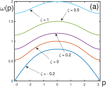
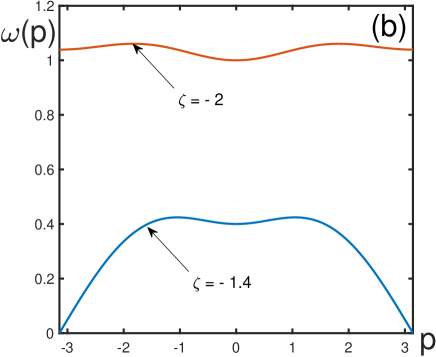
Figure 1: Dimensionless spectrum of spin waves $\omega(p)$ as a function of the dimensionless transverse momentum $p$, under the positive average spin polarization $S_{0}=1$ and the dimensionless strength of dipolar interactions $\gamma_{D}=0.1$, for different dimensionless parameters of the quadratic Zeeman effect $\zeta$. The spectrum is stable for $\zeta\geq-0.2$ (Fig. 1a) and $\zeta\leq-1.4$ (Fig. 1b).

         

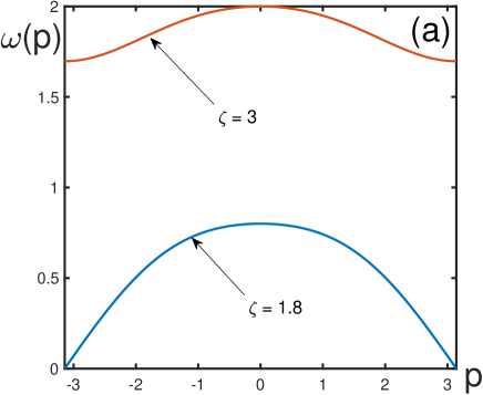
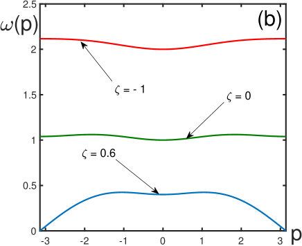
Figure 2: Dimensionless spectrum of spin waves as a function of the dimensionless transverse momentum, under the negative spin polarization $S_{0}=-1$ and $\gamma_{D}=0.1$, for different quadratic Zeeman-effect parameters $\zeta$. The spectrum is stable for either $\zeta\geq 1.8$ (Fig. 2a) or $\zeta\leq 0.6$ (Fig. 2b).

References

- [1] H. Yu, J. Xiao, P. Pirro, Magnon spintronics, J. Magn. Magn. Mater. 450 (2018) 1–2.
- [2] A.I. Akhiezer, V.G. Bariakhtar, S.V. Peletminsky, Spin Waves, Academic, New York, 1967.
- [3] O. Kahn, Molecular Magnetism, VCH, New York, 1995.
- [4] B. Barbara, L. Thomas, F. Lionti, I. Chiorescu, A. Sulpice, Macroscopic quantum tunneling in molecular magnets, J. Magn. Magn. Mater. 200 (1999) 167–181.
- [5] A. Caneschi, D. Gatteschi, C. Sangregorio, R. Sessoli, L. Sorace, A. Cornia, M.A. Novak, C. Paulsen, W. Wernsdorfer, The molecular approach to nanoscale magnetism, J. Magn. Magn. Mater. 200 (1999) 182–201
- [6] V.I. Yukalov, Superradiant operation of spin masers, Laser Phys. 12 (2002) 1089–1103.
- [7] V.I. Yukalov and E.P. Yukalova, Coherent nuclear radiation, Phys. Part. Nucl. 35 (2004) 348–382.
- [8] V.I. Yukalov, V.K. Henner, P.V. Kharebov, Coherent spin relaxation in moleculat magnets, Phys. Rev. B 77 (2008) 134427
- [9] R.H. Kodama, Magnetic nanoparticles, J. Magn. Magn. Mater. 200 (1999) 359–372.
- [10] G.C. Hadjipanayis, Nanophase hard magnets, J. Magn. Magn. Mater. 200 (1999) 373–391.
- [11] V.I. Yukalov, E.P. Yukalova, Possibility of superradiance by magnetic nanoclusters, Laser Phys. Lett. 8 (2011) 804–813.
- [12] V.I. Yukalov, Nonlinear spin dynamics in nuclear magnets, Phys. Rev. B 53 (1996) 9232–9250.
- [13] G.L. Viali, G.R. Gonçalves, E.C. Passamani, J.C.C. Freitas, M.A. Schettino, A.Y. Takeuchi, C. Larica, Magnetic and hyperfine properties of Fe2P nanoparticles dispersed in a porous carbon matrix, J. Magn. Magn. Mater. 401 (2016) 173–179.
- [14] A. Griesmaier, Generation of a dipolar Bose-Einstein condensate, J. Phys. B 40 (2007) R91–R134.
- [15] M.A. Baranov, Theoretical progress in many-body physics with ultracold dipolar gases, Phys. Rep. 464 (2008) 71–111.
- [16] M.A. Baranov, M. Dalmonte, G. Pupillo, P. Zoller, Condensed matter theory of dipolar quantum gases, Chem. Rev. 112 (2012) 5012–5061.
- [17] B. Gadway, B. Yan, Strongly interacting ultracold polar molecules, J. Phys. B 49 (2016) 152002.
- [18] V.I. Yukalov, Dipolar and spinor bosonic systems, Laser Phys. 28 (2018) 053001.
- [19] L.F. Cameretti, Modeling of Thermodynamic Properties in Biological Solutions, Cuviller, Göttingen, 2009.
- [20] T.A. Waigh, The Physics of Living Processes, Wiley, Chichester, 2014.
- [21] W. Barford, Electronic and Optical Properties of Conjugated Polymers, Oxford University, Oxford, 2013.
- [22] G.K. Woodgate, Elementary Atomic Structure, Oxford University, Oxford, 1999.
- [23] W. Demtröder, Molecular Physics, Wiley, Berlin, 2005.
- [24] F. A. Jenkins, E. Segre, The quadratic Zeeman effect, Phys. Rev. 59 (1939) 52–58.
- [25] L. I. Schiff, H. Snyder, Theory of the quadratic Zeeman effect, Phys. Rev. 59 (1939) 59–62.
- [26] J. Killingbeck, The quadratic Zeeman effect, J. Phys. B 12 (1979) 25–30.
- [27] S.L. Coffey, A. Deprit, B. Miller, C.A. Williams, The quadratic Zeeman effect in moderately strong magnetic fields, New York Acad. Sci. 497 (1987) 22–36.
- [28] K.T. Taylor, M.H. Nayfeh, C.W. Clark, eds., Atomic Spectra and Collisions in External Fields, Plenum, New York, 1988.
- [29] D.M. Stamper-Kurn, M. Ueda, Spinor Bose gases: symmetries, magnetism, and quantum dynamics, Rev. Mod. Phys. 85 (2013) 1191–1244.
- [30] B. Pajot, F. Merlet , G. Taravella, P. Arcas, Quadratic Zeeman effect of donor lines in Silicon and Germanium, Can. J. Phys. 50 (1972) 1106–1113.
- [31] L. Veissier, C.W. Thiel, T. Lutz, P.E. Barclay, W. Tittel, R.L. Cone, Quadratic Zeeman effect and spin-lattice relaxation of Tm3+: YAG at high magnetic fields, Phys. Rev. B 94 (2016) 205133.
- [32] J.L. Birman, R.G. Nazmitdinov, V.I. Yukalov, Effects of symmetry breaking in finite quantum systems, Phys. Rep. 526 (2013) 1–91.
- [33] S.J. Prado, C. Trallero-Giner, A.M. Alcalde, V. Lopez–Richard, G.E. Marques, Magneto-optical properties of nanocrystals: Zeeman splitting, Phys. Rev. B 67 (2003) 165306.
- [34] C. Cohen-Tannoudji, J. Dupon-Roc, Experimental study of Zeeman light shifts in weak magnetic fields, Phys. Rev. A 5 (1972) 968–984.
- [35] L. Santos, M. Fattori, J. Stuhler, T. Pfau, Spinor condensates with a laser-induced quadratic Zeeman effect, Phys. Rev. A 75 (2007) 053606.
- [36] K. Jensen, V.M. Acosta, J.M. Higbie, M.P. Ledbetter, S.M. Rochester, D. Budker Cancellation of nonlinear Zeeman shifts with light shifts, Phys. Rev. A 79 (2009) 023406.
- [37] A. de Paz, A. Sharma, A. Chotia, E. Marechal, J. Huckans, P. Pedri, L. Santos, O. Gorceix, L. Vernac, B. Laburthe-Tolra, Nonequilibrium quantum magnetism in a dipolar lattice gas, Phys. Rev. Lett. 111 (2013) 185305.
- [38] F. Gerbier, A. Widera, S. Folling, O. Mandel, I. Bloch, Resonant control of spin dynamics in ultracold quantum gases by microwave dressing, Phys. Rev. A 73 (2006) 041602.
- [39] S.R. Leslie, J. Guzman, M. Vengalattore, J.D. Sau, M.L. Cohen, D.M. Stamper-Kurn, Amplification of fluctuations in a spinor Bose-Einstein condensate, Phys. Rev. A 79 (2009) 043631.
- [40] E.M. Bookjans, A. Vinit, C. Raman, Quantum phase transition in an antiferromagnetic spinor Bose-Einstein condensate, Phys. Rev. Lett. 107 (2011) 195306.
- [41] A.K. Jonscher, Universal Relaxation Rate, Chelsea Dielectrics, London, 1996.
- [42] A.K. Jonscher, Dielectric relaxation with dipolar screening, J. Mater. Sci. 32 (1997) 6409–6414.
- [43] A.K. Jonscher, Low–loss dielectrics, J. Mater. Sci. 34 (1999) 3071–3082.
- [44] V.E. Tarasov, Universal electromagnetic waves in dielectric J. Phys. Condens. Matter 20 (2008) 175223.
- [45] V.I. Yukalov, Bose-condensed atomic systems with nonlocal interaction potentials, Laser Phys. 26 (2016) 045501.
- [46] S.V. Tyablikov, Methods in Quantum Theory of Magnetism, Springer, Berlin, 1995.
- [47] V.I. Yukalov, Nonlinear spin relaxation in strongly nonequilibrium magnets, Phys. Rev. B 71 (2005) 184432.
- [48] V.I. Yukalov, Origin of pure spin superradiance. Phys. Rev. Lett. 75 (1995) 3000–3003.
- [49] V.I. Yukalov, E.P. Yukalova, Processing information by punctuated spin superradiance. Phys. Rev. Lett. 88 (2002) 257601.
- [50] B. Gadway, B. Yan, Srongly interacting ultracold polar molecules, J. Phys. B 49 (2016) 152002.