Recently new solvable systems of nonlinear evolution equations—including ODEs, PDEs and systems with discrete time—have been introduced. These findings are based on certain convenient formulas expressing the $k$-th time-derivative of a root of a time-dependent monic polynomial in terms of the $k$-th time-derivative of the coefficients of the same polynomial and of the roots of the same polynomial as well as their time-derivatives of order less than $k$. These findings were restricted to the case of generic polynomials without any multiple root. In this paper some of these findings—those for $k=1$ and $k=2$—are extended to polynomials featuring one double root; and a few representative examples are reported of new solvable systems of nonlinear evolution equations.

Keywords: solvable systems, nonlinear evolution equations, $N$-body problems, many-body problems, isochronous systems, completely periodic solutions, goldfish type systems.

MSC: 70F10, 70K42

1 Introduction

Recently new classes of systems of solvable evolution equations—including ordinary differential equations (ODEs), partial differential equations (PDEs) and systems evolving in discrete time—have been identified [1]-[14]. The basic idea of these recent developments is quite simple and rather old. Consider a time-dependent monic polynomial of degree $N$ in the complex variable $z$, which is then characterized by $N$ time-dependent coefficients $y_{m}\left(t\right)$ and $N$ zeros $x_{n}\left(t\right).$ [Here and hereafter $N$ is a fixed positive integer larger than unity ($N\geq 2$), indices such as $m$ and $n$ range over the integers from $1$ to $N$ unless otherwise indicated, the real variable $t$ is “time”, superimposed dots indicate time-differentiations, and all other quantities are generally complex numbers]. Assume then that the time evolution of the $N$ coefficients $y_{m}\left(t\right)$ of this polynomial evolve in time according to equations of motion which are in some sense “solvable”—for instance by algebraic operations, or via some other appropriate and convenient technique. It is then often the case that these evolutions are, in some sense, “simple and interesting”: for instance, Hamiltonian and possibly integrable and/or multiply periodic, completely periodic or even isochronous. Look then at the corresponding evolution of the $N$ zeros $x_{n}\left(t\right)$. It is generally more complicated (“more nonlinear”), yet it generally inherits the properties of the evolution of the coefficients $y_{m}\left(t\right)$: hence it is, in some sense, also “simple and interesting”, therefore worth of identification and further study. This approach was introduced 4 decades ago [15]-[17] to identify integrable/solvable many-body problems characterized by evolution equations of Newtonian type—“accelerations equal forces”—describing $N$ points moving in the complex plane (or equivalently in the real plane) identified with the $N$ zeros $x_{n}\left(t\right)$ of time-dependent monic polynomials the $N$ coefficients $y_{m}\left(t\right)$ of which evolve in time according to a system of linear ODEs. At the time this restriction to a linear evolution of the coefficients was essential in order to be able to write explicitly the corresponding evolution of the zeros. Only recently a simple technique has been introduced [1] [7], which allows to obtain in explicit form the equations of motion of the zeros of a time-dependent monic polynomial the coefficients of which evolve according to nonlinear equations of motion. This opened the way to the identification and investigation of large classes of new solvable nonlinear evolution equations, as mentioned above [1]-[14].

This development was however restricted so far to the consideration of generic time-dependent polynomials, the zeros of which are all different among themselves, except possibly at some special times corresponding to collisions of some of the moving zeros.

In the present paper a first step is made towards the elimination of this restriction, by considering polynomials which feature one double zero, opening thereby the possibility to identify additional classes of nonlinear evolution amenable to exact treatments; and some such examples are reported.

This generalization is described in the following Section 2, and some examples of new systems of solvable nonlinear evolution equations are identified and investigated in Section 3. The last Section 4 (“Outlook”) provides a terse overview of further developments.

2 Monic time-dependent polynomials with one double root, and related formulas

In this Section 2 we report and prove formulas—of a type which is particularly convenient for the identification and investigation of new solvable evolution equations [1]-[14]—which relate the time evolution of the zeros of a (nongeneric) monic polynomial featuring—for all time—one double zero, to the time-evolution of its coefficients. This Section 2 is divided into 2 Subsections, in which we treat this problem in order of increasing complexity: in Subsection 2.1, the simplest problem of a time-dependent polynomial of third degree with a double zero; and in Subsection 2.2, the case of a time-dependent polynomial of arbitrary degree $N+1$ with one double zero. The extension of these findings to the most general case—a time-dependent polynomial of arbitrary degree featuring several zeros of arbitrary multiplicities—is a nontrivial undertaking: this task shall eventually be treated—by ourselves or by others—in subsequent publications.

2.1 The monic time-dependent polynomial of third degree with a double zero, and related formulas

It is convenient to start from the simplest case, that of a monic polynomial of degree $3$ featuring a double zero:

$$p_{3}\left(z;t\right)=z^{3}+y_{1}\left(t\right)~{}z^{2}+y_{2}\left(t\right)~{}z+y_{3}\left(t\right)~{},$$ (1a)

$$p_{3}\left(z;t\right)=\left[z-x_{1}\left(t\right)\right]^{2}~{}\left[z-x_{2}\left(t\right)\right]~{}.$$ (1b)

Indeed, this case is simple enough to write the relevant formulas without explanations, yet it is sufficient to highlight the complications that make the case with multiple zeros rather different from the case of generic polynomials—hence, featuring no multiple zeros—previously treated [1]-[14].

Hereafter the explicit indication of the time-dependence of the various quantities will be omitted whenever we feel that this omission—even if, occasionally, applied inconsistently within the same formula—is unlikely to cause misunderstandings.

The 3 coefficients $y_{1},~{}y_{2},~{}y_{3}$ are of course given by the following formulas in terms of the two zeros $x_{1}$ and $x_{2}$:

$$y_{1}=-\left(2~{}x_{1}+x_{2}\right)~{},~{}~{}y_{2}=\left(x_{1}\right)^{2}+2~{}x_{1}~{}x_{2}~{},~{}~{}y_{3}=-\left(x_{1}\right)^{2}~{}x_{2}~{};$$ (2a)

and these equations imply the following expressions of the time derivatives $$\dot{y}_{m}$$:

$$\dot{y}_{1} = -\left(2~{}\dot{x}_{1}+\dot{x}_{2}\right)~{},~{}~{}~{}\dot{y}_{2}=2~{}\left[\dot{x}_{1}~{}\left(x_{1}+x_{2}\right)+\dot{x}_{2}~{}x_{1}\right]~{},$$

$$\dot{y}_{3} = -\left[2~{}\dot{x}_{1}~{}x_{1}~{}x_{2}+\dot{x}_{2}~{}\left(x_{1}\right)^{2}\right]~{}.$$ (2b)

There hold moreover the following formulas:

$$p_{3}\left(x_{n};t\right)=\left(x_{n}\right)^{3}+y_{1}~{}\left(x_{n}\right)^{2}+y_{2}~{}x_{n}+y_{3}=0~{},~{}~{}~{}n=1,2~{};$$ (3)

$$p_{3,z}\left(z;t\right)=3~{}z^{2}+2~{}y_{1}~{}z+y_{2}$$ (4)

$$= 2~{}\left(z-x_{1}\right)~{}\left(z-x_{2}\right)+\left(z-x_{1}\right)^{2}~{},$$

$$p_{3,t}\left(z;t\right)=\dot{y}_{1}~{}z^{2}+\dot{y}_{2}~{}z+\dot{y}_{3}$$ (5)

$$= -2~{}\dot{x}_{1}~{}\left(z-x_{1}\right)~{}\left(z-x_{2}\right)-\dot{x}_{2}~{}\left(z-x_{1}\right)^{2}~{}.$$

Above and hereafter appended variables preceded by a comma denote (partial) differentiations with respect to that variable.

For $z=x_{1}$ respectively for $z=x_{2}$ the last $2$ formulas yield the following relations:

$$3~{}\left(x_{1}\right)^{2}+2~{}y_{1}~{}x_{1}+y_{2}=0~{},$$ (6a)

$$3~{}\left(x_{2}\right)^{2}+2~{}y_{1}~{}x_{2}+y_{2}=\left(x_{1}-x_{2}\right)^{2}~{};$$ (6b)

$$\dot{y}_{1}~{}\left(x_{1}\right)^{2}+\dot{y}_{2}~{}x_{1}+\dot{y}_{3}=0~{},$$ (7a)

$$\dot{y}_{1}~{}\left(x_{2}\right)^{2}+\dot{y}_{2}~{}x_{2}+\dot{y}_{3}=-\dot{x}_{2}~{}\left(x_{1}-x_{2}\right)^{2}~{}.$$ (7b)

It is then a matter of trivial algebra to obtain the following $3$ (different!) systems of evolution equations, which relate the time evolution of the $2$ zeros $x_{1}\left(t\right)$ and $x_{2}\left(t\right)$ to the evolution of $2$ out of the $3$ coefficients $y_{1}\left(t\right),~{}y_{2}\left(t\right),~{}y_{3}\left(t\right)$:

$$\dot{x}_{1}=-\frac{2~{}x_{1}~{}\dot{y}_{1}+\dot{y}_{2}}{2~{}\left(x_{1}-x_{2}\right)}~{},~{}~{}~{}\dot{x}_{2}=\frac{\left(x_{1}+x_{2}\right)~{}\dot{y}_{1}+\dot{y}_{2}}{x_{1}-x_{2}}~{};$$ (8)

$$\dot{x}_{1}=-\frac{\left(x_{1}\right)^{2}~{}\dot{y}_{1}-\dot{y}_{3}}{2~{}x_{1}~{}\left(x_{1}-x_{2}\right)}~{},~{}~{}~{}\dot{x}_{2}=\frac{x_{1}~{}x_{2}~{}\dot{y}_{1}-\dot{y}_{3}}{x_{1}~{}\left(x_{1}-x_{2}\right)}~{};$$ (9)

$$\dot{x}_{1}=\frac{x_{1}~{}\dot{y}_{2}+2~{}\dot{y}_{3}}{2~{}x_{1}~{}\left(x_{1}-x_{2}\right)}~{},~{}~{}~{}\dot{x}_{2}=-\frac{x_{1}~{}x_{2}~{}\dot{y}_{2}+\left(x_{1}+x_{2}\right)~{}\dot{y}_{3}}{\left(x_{1}\right)^{2}~{}\left(x_{1}-x_{2}\right)}~{}.$$ (10)

Analogous equations can be obtained for higher-order time-derivatives; the relevant expressions become progressively more complicated as the order of differentiation increases. Here we report the equations for the second time-derivatives, in view of their relevance in the study of many-body dynamics due to their relations to the Newtonian equations of motion of classical mechanics (“accelerations equal forces”). They read as follows:

$$\ddot{x}_{1}=\frac{2~{}\dot{x}_{1}~{}\left(\dot{x}_{1}+2~{}\dot{x}_{2}\right)-2~{}x_{1}~{}\ddot{y}_{1}-\ddot{y}_{2}}{2~{}\left(x_{1}-x_{2}\right)}~{},$$

$$\ddot{x}_{2}=\frac{-2~{}\dot{x}_{1}~{}\left(\dot{x}_{1}+2~{}\dot{x}_{2}\right)+\left(x_{1}+x_{2}\right)~{}\ddot{y}_{1}+\ddot{y}_{2}}{x_{1}-x_{2}}~{};$$ (11)

$$\ddot{x}_{1}=\frac{2~{}\dot{x}_{1}~{}\left(\dot{x}_{1}~{}x_{2}+2~{}\dot{x}_{2}~{}x_{1}\right)-\left(x_{1}\right)^{2}~{}\ddot{y}_{1}+\ddot{y}_{3}}{2~{}x_{1}~{}\left(x_{1}-x_{2}\right)}~{},$$

$$\ddot{x}_{2}=\frac{-2~{}\dot{x}_{1}~{}\left(\dot{x}_{1}~{}x_{2}+2~{}\dot{x}_{2}~{}x_{1}\right)+x_{1}~{}x_{2}~{}\ddot{y}_{1}-\ddot{y}_{3}}{x_{1}~{}\left(x_{1}-x_{2}\right)}~{};$$ (12)

$$\ddot{x}_{1}=\frac{-2~{}x_{1}~{}\dot{x}_{1}~{}\left(\dot{x}_{1}-2~{}\dot{x}_{2}\right)+4~{}\left(\dot{x}_{1}\right)^{2}~{}x_{2}+x_{1}~{}\ddot{y}_{2}+2~{}\ddot{y}_{3}}{2~{}x_{1}~{}\left(x_{1}-x_{2}\right)}~{},$$

$$\ddot{x}_{2}=-\frac{2~{}\dot{x}_{1}~{}\left[\dot{x}_{1}~{}\left(x_{2}\right)^{2}+2~{}\dot{x}_{2}~{}\left(x_{1}~{}\right)^{2}\right]+x_{1}~{}x_{2}~{}\ddot{y}_{2}+\left(x_{1}+x_{2}\right)~{}\ddot{y}_{3}}{\left(x_{1}\right)^{2}~{}\left(x_{1}-x_{2}\right)}~{}.$$ (13)

These $3$ (different!) systems of $2$ coupled ODEs provide the tools to identify and investigate new systems of $2$ equations of motions of potential theoretical or applicative interest (although they have been mainly discussed here to introduce the treatment of analogous—but more general—new systems of $N$ nonlinear evolution equations). The idea—as in [1]-[17]—is to assume that $2$ of the $3$ quantities $y_{m}\left(t\right)$ evolve in time according to a system of evolution equations amenable to exact treatments; say

$$\ddot{y}_{1}=f_{1}\left(\dot{y}_{1},~{}\dot{y}_{2};~{}y_{1},~{}y_{2}\right)~{},~{}~{}~{}\ddot{y}_{2}=f_{2}\left(\dot{y}_{1},~{}\dot{y}_{2};~{}y_{1},~{}y_{2}\right)~{},$$ (14)

with the $2$ functions $f_{1}\left(\dot{y}_{1},~{}\dot{y}_{2};~{}y_{1},~{}y_{2}\right)$ and $f_{2}\left(\dot{y}_{1},~{}\dot{y}_{2};~{}y_{1},~{}y_{2}\right)$ such that this system can be explicitly solved (see examples in Section 3). Then, by inserting these expressions in the right hand side of system (11), one obtains the following system of $2$, generally highly nonlinear, evolution equations:

$$\ddot{x}_{1} = \frac{1}{2}~{}\left(x_{1}-x_{2}\right)^{-1}\Big{[}2~{}\dot{x}_{1}~{}\left(\dot{x}_{1}+2~{}\dot{x}_{2}\right)-2~{}x_{1}~{}f_{1}\left(\dot{y}_{1},~{}\dot{y}_{2};~{}y_{1},~{}y_{2}\right)$$

$$-f_{2}\left(\dot{y}_{1},~{}\dot{y}_{2};~{}y_{1},~{}y_{2}\right)\Big{]}~{},$$

$$\ddot{x}_{2} = (x_{1}-x_{2})^{-1}\Big{[}-2~{}\dot{x}_{1}~{}\left(\dot{x}_{1}+2~{}\dot{x}_{2}\right)+\left(x_{1}+x_{2}\right)~{}f_{1}\left(\dot{y}_{1},~{}\dot{y}_{2};~{}y_{1},~{}y_{2}\right)$$ (15)

$$+f_{2}\left(\dot{y}_{1},~{}\dot{y}_{2};~{}y_{1},~{}y_{2}\right)\Big{]}~{}$$

with, in the right-hand sides, the quantities $\dot{y}_{1},~{}\dot{y}_{2},~{}y_{1},~{}y_{2}$ replaced by their explicit expressions (see (2b) and (2a)) in terms of $x_{1}$ and $x_{2}$ and their time derivatives. This is then one of the $3$ new solvable systems of $2$ nonlinearly coupled second-order (“Newtonian”) equations of motion satisfied by the quantities $x_{1}\left(t\right)$ and $x_{2}\left(t\right)$ (the other two such systems obtain of course in an analogous manner from (12) and (13) rather than (11); see below). Let us now explain how the solution of this $2$-body problem, (15), can be achieved.

Step (i). Given the initial values $x_{n}\left(0\right)$ of the $2$ zeros $x_{n}\left(t\right)$ as well as the initial values of their velocities, via the formulas (2a) and (2b) the initial values $y_{m}\left(0\right)$ and $\dot{y}_{m}\left(0\right)$ with $m=1,2,3$ are (easily) computed.

Step (ii). From the initial values $y_{m}\left(0\right)$ and $\dot{y}_{m}\left(0\right)$ with $m=1,2$ the values of $y_{m}\left(t\right)$—and then as well of $\dot{y}_{m}\left(t\right)$—are computed by solving the—assumedly solvable—system of evolution equations (14).

Step (iii). From the knowledge of $y_{1}\left(t\right)$ and $y_{2}\left(t\right)$ the value of $x_{1}\left(t\right)$ is computed by solving the quadratic equation (6a). There obtain, for every value of $t,$ two different values of $x_{1}\left(t\right);$ and by following them, by continuity in $t,$ all the way back to $t=0$—and by comparing the value $x_{1}\left(0\right)$ yielded by this procedure with the initial datum $x_{1}\left(0\right)$—the actual (continuous) solution $x_{1}\left(t\right)$ is identified.

Step (iv). The solution $x_{2}\left(t\right)$ for all time is then immediately obtained, for instance, from the known functions $x_{1}\left(t\right)$ and $y_{1}\left(t\right),$ via the first of the $3$ equations (2a).

The way to solve the other two systems, (12) and (13), is analogous but not quite identical, so let us tersely detail how the method works for the second system (12).

So, we now take as point of departure the system

$$\ddot{y}_{1}=f_{1}\left(\dot{y}_{1},~{}\dot{y}_{3};~{}y_{1},~{}y_{3}\right)~{},~{}~{}~{}\ddot{y}_{3}=f_{3}\left(\dot{y}_{1},~{}\dot{y}_{3};~{}y_{1},~{}y_{3}\right)~{},$$ (16)

with the $2$ functions $f_{1}\left(\dot{y}_{1},~{}\dot{y}_{3};~{}y_{1},~{}y_{3}\right)$ and $f_{3}\left(\dot{y}_{1},~{}\dot{y}_{3};~{}y_{1},~{}y_{3}\right)$ such that this system can be explicitly solved (see examples below). Then, by inserting these expressions in the right hand side of the system (11), one obtains the following system of $2$, generally highly nonlinear, evolution equations:

$$\ddot{x}_{1} = \left[2x_{1}\left(x_{1}-x_{2}\right)\right]^{-1}\Big{[}2~{}\dot{x}_{1}~{}\left(\dot{x}_{1}~{}x_{2}+2~{}\dot{x}_{2}~{}x_{1}\right)-\left(x_{1}\right)^{2}~{}f_{1}\left(\dot{y}_{1},~{}\dot{y}_{3};~{}y_{1},~{}y_{3}\right)$$

$$+f_{3}\left(\dot{y}_{1},~{}\dot{y}_{3};~{}y_{1},~{}y_{3}\right)\Big{]}~{},$$

$$\ddot{x}_{2} = \left[x_{1}\left(x_{1}-x_{2}\right)\right]^{-1}\Big{[}-2~{}\dot{x}_{1}~{}\left(\dot{x}_{1}~{}x_{2}+2~{}\dot{x}_{2}~{}x_{1}\right)+x_{1}~{}x_{2}~{}f_{1}\left(\dot{y}_{1},~{}\dot{y}_{3};~{}y_{1},~{}y_{3}\right)$$ (17)

$$-f_{3}\left(\dot{y}_{1},~{}\dot{y}_{3};~{}y_{1},~{}y_{3}\right)\Big{]}~{};$$

with, in the right-hand sides, the quantities $\dot{y}_{1},~{}\dot{y}_{3},~{}y_{1},~{}y_{3}$ replaced by their explicit expressions (see (2b) and (2a)) in terms of $x_{1}$ and $x_{2}$ and their time derivatives. This is then the second one of the $3$ new solvable systems of $2$ nonlinearly coupled second-order (“Newtonian”) equations of motion satisfied by the quantities $x_{1}\left(t\right)$ and $x_{2}\left(t\right)$.

Let us now explain how the solution of this $2$-body problem, (17), can be achieved.

Step (i). Given the initial values $x_{n}\left(0\right)$ of the $2$ zeros $x_{n}\left(t\right)$ as well as the initial values of their velocities, via the formulas (2a) and (2b) the initial values $y_{m}\left(0\right)$ and $\dot{y}_{m}\left(0\right)$ with $m=1,2,3$ are (easily) computed.

Step (ii). From the initial values $y_{m}\left(0\right)$ and $\dot{y}_{m}\left(0\right)$ with $m=1,3$ the values of $y_{m}\left(t\right)$—and then as well of $\dot{y}_{m}\left(t\right)$—are computed by solving the—assumedly solvable—system of evolution equations (16).

Step (iii). From the knowledge of $y_{1}\left(t\right)$ and $y_{3}\left(t\right)$ the value of $x_{1}\left(t\right)$ is computed as the root of the cubic equation

$$2~{}\left(x_{1}\right)^{3}+y_{1}~{}\left(x_{1}\right)^{2}-y_{3}=0~{},$$ (18)

which is implied by (6a) via the first of the $3$ equations (2a). By solving this cubic equation there obtain, for every value of $t,$ three different values of $x_{1}\left(t\right);$ and by following them, by continuity in $t,$ all the way back to $t=0$—and by then comparing the value $x_{1}\left(0\right)$ yielded by this procedure with the initial datum $x_{1}\left(0\right)$—the actual (continuous) solution $x_{1}\left(t\right)$ is identified.

Step (iv). The solution $x_{2}\left(t\right)$ for all time is then immediately obtained, for instance, from the known functions $x_{1}\left(t\right)$ and $y_{1}\left(t\right),$ via the first of the $3$ equations (2a).

The treatment of the third of the $3$ solvable systems the equations of motion of which read

$$\ddot{x}_{1}=\left[2~{}x_{1}~{}\left(x_{1}-x_{2}\right)\right]^{-1}~{}\Big{[}-2~{}x_{1}~{}\dot{x}_{1}~{}\left(\dot{x}_{1}-2~{}\dot{x}_{2}\right)+4~{}\left(\dot{x}_{1}\right)^{2}~{}x_{2}$$

$$+x_{1}~{}f_{2}\left(\dot{y}_{2},~{}\dot{y}_{3};~{}y_{2},~{}y_{3}\right)+2~{}f_{3}\left(\dot{y}_{2},~{}\dot{y}_{3};~{}y_{2},~{}y_{3}\right)\Big{]}~{},$$

$$\ddot{x}_{2}=-\left[\left(x_{1}\right)^{2}~{}\left(x_{1}-x_{2}\right)\right]^{-1}~{}\Big{\{}2~{}\dot{x}_{1}~{}\left[\dot{x}_{1}~{}\left(x_{2}\right)^{2}+2~{}\dot{x}_{2}~{}\left(x_{1}~{}\right)^{2}\right]$$

$$+x_{1}~{}x_{2}~{}f_{2}\left(\dot{y}_{2},~{}\dot{y}_{3};~{}y_{2},~{}y_{3}\right)+\left(x_{1}+x_{2}\right)~{}f_{3}\left(\dot{y}_{2},~{}\dot{y}_{3};~{}y_{2},~{}y_{3}\right)\Big{\}}~{},$$ (19)

—corresponding to the equations of motion

$$\ddot{y}_{2}=f_{2}\left(\dot{y}_{2},~{}\dot{y}_{3};~{}y_{2},~{}y_{3}\right)~{},~{}~{}~{}\ddot{y}_{3}=f_{3}\left(\dot{y}_{2},~{}\dot{y}_{3};~{}y_{2},~{}y_{3}\right)$$ (20)

—is quite analogous, except for Step (iii), that now requires solving the following cubic equation to determine $x_{1}\left(t\right)$ in terms of $y_{2}\left(t\right)$ and $y_{3}\left(t\right)$:

$$\left(x_{1}\right)^{3}-x_{1}~{}y_{2}-2~{}y_{3}=0~{}.$$ (21)

It is plain from this treatment—see, if need be, the detailed discussions of this question in [1]-[17]—that the $3$ two-body problems (15), (17) respectively (19) “inherit” all the nice properties—such as the property to be Hamiltonian, the property of integrability in the Hamiltonian context, and various periodicity properties including isochrony and asymptotic isochrony—possibly possessed by the solvable systems (14), (16) respectively (20). Some specific examples are reported in Subsection 3.1

2.2 The monic time-dependent polynomial of degree $N+1$ with a double zero, and related formulas

The monic time-dependent polynomial of degree $N+1$ featuring $N+1$ coefficients and $N$ zeros, one of which is double, reads as follows:

$$p_{N+1}\left(z;t\right)=z^{N+1}+\sum_{m=1}^{N+1}\left[y_{m}\left(t\right)~{}z^{N+1-m}\right]~{},$$ (22a)

$$p_{N+1}\left(z;t\right)=\left[z-x_{1}\left(t\right)\right]^{2}~{}\mathop{\displaystyle\prod}\limits_{n=2}^{N}\left[z-x_{n}\left(t\right)\right]~{}.$$ (22b)

Note that it features $$N+1 y_{m}\left(t\right) m=1,2,...,N+1 N x_{n}\left(t\right) n=1,2,...,N 2 x_{1}\left(t\right) N+1 y_{m}\left(t\right) t, t x_{n}=x_{n}(t) y_{m}=y_{m}(t).$$ coefficients (with , see (22a)) and zeros (with , see (22b)); all but one of these zeros have unit multiplicity, the exceptional one having multiplicity and being identified as . This of course implies that the coefficients are, for all time related to each other by one constraint (see below). As in the previous section, we will occasionally omit the explicit indication of the -dependence of and

These formulas, (22), imply of course that the $N+1$ coefficients $y_{m}$ are expressed in terms of the $N$ zeros $x_{n}$ by the standard formulas

$$y_{m}=\left(-1\right)^{m}~{}\sigma_{m}\left(\tilde{x}\right)~{},$$ (23a)

where $$\sigma_{m}\left(\tilde{x}\right) m N+1 \tilde{x} \left(x_{1},~{}x_{1},~{}x_{2},...,~{}x_{N}\right) N+1 p_{N+1}\left(z;t\right) x_{1} N x_{n}$$ is the standard symmetric polynomial of degree in variables, evaluated at any permutation of the vector of the zeros of with repeated twice. For instance, the first and last of these coefficients are expressed in terms of the zeros as follows:

$$y_{1}=-\left(2~{}x_{1}+x_{2}+x_{3}+...+x_{N}\right)~{},$$ (23b)

$$y_{N+1}=\left(-\right)^{N+1}\left(x_{1}\right)^{2}~{}x_{2}~{}x_{3}...x_{N}~{}.$$ (23c)

Conversely—once the polynomial $$p_{N+1}\left(z\right) N+1 y_{m} N x_{n} N-1 x_{2},~{}x_{3},~{}...,~{}x_{N} N+1 y_{m} N N x_{n} n=1,2,...,N N y_{m} y_{\bar{m}} \bar{m} 1 N+1 N y_{m} m=1,2,...,\bar{m}-1,\bar{m}+1,...,N,N+1 y_{\bar{m}} \bar{m} 1 N+1. \dot{x}_{n}\left(t\right) \ddot{x}_{n}\left(t\right) n 1 N \dot{y}_{m}\left(t\right) \ddot{y}_{m}\left(t\right), N y_{m}\left(t\right) m=1,2,...,\bar{m}-1,\bar{m}+1,...,N+1 N+1 y_{m}\left(t\right) y_{\bar{m}}\left(t\right) N x_{n} n=1,2,...,N y_{\bar{m}} N y_{m} m=1,2,...\bar{m}-1,~{}\bar{m}+1,...N+1$$ has been assigned via its coefficients —then its zeros are uniquely determined (up to permutations of the zeros ). They can therefore be obtained from the coefficients by algebraic operations, which however can generally be explicitly performed only for small values of . But a more relevant issue for our purposes—which is treated at the end of this Subsection 2.2—is to show how the zeros with of the polynomial (22), as well as one of the coefficients —say, the coefficient , with an arbitrarily assigned integer in the range from to —can be obtained by algebraic operations from the coefficients with of this polynomial (22) (taking of course advantage of the fact that this polynomial features a double zero). Note the special role (not!) played by the coefficient , with an arbitrarily assigned integer in the range from to Our task is to derive convenient expressions of the first respectively the second time derivative, respectively (for every given in the range from to ), in terms of the first respectively the second derivatives, respectively of the coefficients with (hence of all the coefficients with the exclusion of the special coefficient ). At the end of this section we also discuss how the zeros with of the polynomial (22), as well as the coefficient of this polynomial, can be obtained via algebraic operations from the coefficients of this polynomial (22) with (taking of course advantage of the fact that this polynomial features a double zero).

The $t$-derivatives of the two versions, (22a) and (22b) of (22), read of course as follows:

$$p_{N+1,t}\left(z;t\right)=\sum_{m=1}^{N+1}\left[\dot{y}_{m}~{}z^{N+1-m}\right]~{},$$ (24a)

$$p_{N+1,t}\left(z;t\right)=-2~{}\dot{x}_{1}~{}\left(z-x_{1}\right)~{}\mathop{\displaystyle\prod}\limits_{n=2}^{N}\left(z-x_{n}\right)$$

$$-\left(z-x_{1}\right)^{2}~{}\sum_{n=2}^{N}\left[\dot{x}_{n}~{}\mathop{\displaystyle\prod}\limits_{\ell=2,~{}\ell\neq n}^{N}\left(z-x_{\ell}\right)\right]~{}.$$ (24b)

Hence, equating these two formulas for $$z=x_{1}, z=x_{n},$$ respectively for we obtain the following two identities:

$$\sum_{m=1}^{N+1}\left[\dot{y}_{m}~{}\left(x_{1}\right)^{N+1-m}\right]=0~{},$$ (25a)

$$\sum_{m=1}^{N+1}\left[\dot{y}_{m}~{}\left(x_{n}\right)^{N+1-m}\right]$$

$$=-\left(x_{n}-x_{1}\right)^{2}~{}\left[\dot{x}_{n}~{}\mathop{\displaystyle\prod}\limits_{\ell=2,~{}\ell\neq n}^{N}\left(x_{n}-x_{\ell}\right)\right],$$

$$n=2,...,N~{}.$$ (25b)

Then, by subtracting the first of these two formulas multiplied by $$\left(x_{1}\right)^{-\left(N+1-\bar{m}\right)} \left(x_{n}\right)^{-\left(N+1-\bar{m}\right)}$$ from the second multiplied by we obtain the identity

$$-\left(x_{n}-x_{1}\right)^{2}~{}\left[\dot{x}_{n}~{}\mathop{\displaystyle\prod}\limits_{\ell=2,~{}\ell\neq n}^{N}\left(x_{n}-x_{\ell}\right)\right]~{}\left(x_{n}\right)^{-\left(N+1-\bar{m}\right)}$$ (26)

$$= \sum_{m=1}^{N+1}\left\{\dot{y}_{m}~{}\left[\left(x_{n}\right)^{\bar{m}-m}-\left(x_{1}\right)^{\bar{m}-m}\right]\right\}~{},~{}~{}~{}n=2,...,N~{},$$

hence the following expression of the derivatives $\dot{x}_{n}\left(t\right)$ with $n=2,...,N:$

$$\dot{x}_{n}=-\left[\mathop{\displaystyle\prod}\limits_{\ell=1,~{}\ell\neq n}^{N}\left(x_{n}-x_{\ell}\right)^{-1}\right]~{}\left(x_{n}\right)^{N+1-\bar{m}}\cdot$$

$$\cdot\sum_{m=1,~{}m\neq\bar{m}}^{N+1}\left\{\dot{y}_{m}~{}\left[\frac{\left(x_{n}\right)^{\bar{m}-m}-\left(x_{1}\right)^{\bar{m}-m}}{x_{n}-x_{1}}\right]\right\}~{},$$

$$n = 2,...,N~{},$$ (27a)

or, equivalently,

$$\dot{x}_{n}=-\left[\prod_{\ell=1,\ell\neq n}^{N}(x_{n}-x_{\ell})^{-1}\right](x_{n})^{N+1-\bar{m}}$$

$$\Bigg{\{}\sum_{m=1}^{\bar{m}-1}\left[\dot{y}_{m}\sum_{j=0}^{\bar{m}-m-1}(x_{n})^{\bar{m}-m-1-j}(x_{1})^{j}\right]$$

$$-\sum_{m=\bar{m}+1}^{N+1}\left[\dot{y}_{m}\sum_{j=0}^{m-\bar{m}-1}(x_{n})^{\bar{m}-m+j}(x_{1})^{-(j+1)}\right]\Bigg{\}}.$$

$$n=2,\ldots,N.$$ (27b)

This is the first key formula that expresses the first $t$-derivative $\dot{x}_{n}\left(t\right)$ of the $N-1$ zeros $x_{n}\left(t\right)$ (with $n=2,...,N$) in terms of the first $t$-derivatives of the $N~{}$coefficients $y_{m}\left(t\right)$ (with $m\neq\bar{m})$: note that we evidenced the important fact that the quantity $\dot{y}_{m}\left(t\right)$ with $m=\bar{m}$ does not enter in these equations, since for $m=\bar{m}$ the summand in the right-hand side of (27a) clearly vanishes (and the second sum in the right-hand side of (27b) likewise vanishes since it is empty).

Remark 2.1.1. Above and hereafter we assume for simplicity that $x_{1}\left(t\right)$ never vanishes. Since $x_{1}\left(t\right)$ is by definition the double zero of the polynomial (20), clearly a sufficient condition to guarantee this is to restrict attention to time evolutions of the two “highest” coefficients of this polynomial, $y_{N+1}\left(t\right)$ and $y_{N}\left(t\right),$ such that they never vanish simultaneously. $\blacksquare$

Next, let us derive an analogous formula for $\dot{x}_{1}\left(t\right).$ To this end—and also for future developments—we now report the following formulas expressing the first and second $t$-derivative of the first $z$-derivative of the rational functions $z^{\bar{m}-N-1}~{}p_{N+1}\left(z;t\right)$ (see (22a)), which clearly read as follows:

$$\frac{\partial^{2}}{\partial t~{}\partial z}\left[z^{\bar{m}-N-1}~{}p_{N+1}\left(z;t\right)\right]=\sum_{m=1,~{}m\neq\bar{m}}^{N+1}\left[\left(\bar{m}-m\right)~{}\dot{y}_{m}~{}z^{\bar{m}-m-1}\right]~{},$$ (28a)

$$\frac{\partial^{3}}{\partial t^{2}~{}\partial z}\left[z^{\bar{m}-N-1}~{}p_{N+1}\left(z;t\right)\right]=\sum_{m=1,~{}m\neq\bar{m}}^{N+1}\left[\left(\bar{m}-m\right)~{}\ddot{y}_{m}~{}z^{\bar{m}-m-1}\right]~{};$$ (28b)

note that here we again emphasized—by excluding from the sums in the right-hand sides the (vanishing!) term with $$m=\bar{m} y_{\bar{m}}\left(t\right) z=x_{n}\left(t\right) n=1,2,...,N$$—the obvious fact that these formulas are independent of the function . And clearly these formulas, when evaluated at , read—for all values of —as follows:

$$\left.\left\{\frac{\partial^{2}}{\partial t~{}\partial z}\left[z^{\bar{m}-N-1}~{}p_{N+1}\left(z;t\right)\right]\right\}\right|_{z=x_{n}}$$ (29a)

$$= \sum_{m=1,~{}m\neq\bar{m}}^{N+1}\left[\left(\bar{m}-m\right)~{}\dot{y}_{m}~{}\left(x_{n}\right)^{\bar{m}-m-1}\right]~{},$$

$$\left.\left\{\frac{\partial^{3}}{\partial t^{2}~{}\partial z}\left[z^{\bar{m}-N-1}~{}p_{N+1}\left(z;t\right)\right]\right\}\right|_{z=x_{n}}$$ (29b)

$$= \sum_{m=1,~{}m\neq\bar{m}}^{N+1}\left[\left(\bar{m}-m\right)~{}\ddot{y}_{m}~{}\left(x_{n}\right)^{\bar{m}-m-1}\right]~{}.$$

It is on the other hand easily seen that the expressions for the quantities analogous to (29a) that instead follow from the expression (22b) of the polynomial $p_{N+1}\left(z;t\right),$ when evaluated at $z=x_{1}(t)$, read as follows:

$$\left.\left\{\frac{\partial^{2}}{\partial t~{}\partial z}\left[z^{\bar{m}-N-1}~{}p_{N+1}\left(z;t\right)\right]\right\}\right|_{z=x_{1}}$$ (30)

$$= -2~{}\left(x_{1}\right)^{\bar{m}-N-1}~{}\left[\mathop{\textstyle\prod}\limits_{\ell=2}^{N}\left(x_{1}-x_{\ell}\right)\right]~{}\dot{x}_{1}~{}.$$

Equating these equations to (28a)—also evaluated at $z=x_{1}\left(t\right)$—yields the sought expressions of the first derivatives $\dot{x}_{1}$ of the $N$ zero $x_{1}\left(t\right)$:

$$\dot{x}_{1}=\left[2~{}\mathop{\textstyle\prod}\limits_{\ell=2}^{N}\left(x_{1}-x_{\ell}\right)\right]^{-1}~{}\sum_{m=1,~{}m\neq\bar{m}}^{N+1}\left[\left(m-\bar{m}\right)~{}\dot{y}_{m}~{}\left(x_{1}\right)^{N-m}\right]~{}.$$ (31)

In an analogous manner the equations are obtained for the second $t$-derivatives of the $N$ zeros $x_{n}\left(t\right)$ (a check of their derivation is left to the willing reader). They read as follows:

$$\ddot{x}_{1} = -\left(N+1-\bar{m}\right)~{}\frac{\left(\dot{x}_{1}\right)^{2}}{x_{1}}+\dot{x}_{1}~{}\sum_{n=2}^{N}~{}\left(\frac{2~{}\dot{x}_{n}+\dot{x}_{1}}{x_{1}-x_{n}}\right)$$ (32a)

$$+\left[2~{}\mathop{\textstyle\prod}\limits_{n=2}^{N}\left(x_{1}-x_{n}\right)\right]^{-1}\sum_{m=1,~{}m\neq\bar{m}}^{N+1}\left[\left(m-\bar{m}\right)~{}\ddot{y}_{m}~{}\left(x_{1}\right)^{N-m}\right]~{},$$

$$\ddot{x}_{n} = \frac{2~{}\dot{x}_{1}~{}\dot{x}_{n}}{x_{n}-x_{1}}+\sum_{\ell=1,~{}\ell\neq n}^{N}\left(\frac{2~{}\dot{x}_{n}~{}\dot{x}_{\ell}}{x_{n}-x_{\ell}}\right)$$ (32b)

$$+\frac{2~{}\left(\dot{x}_{1}\right)^{2}}{x_{n}-x_{1}}~{}\left(\frac{x_{n}}{x_{1}}\right)^{N+1-\bar{m}}\mathop{\displaystyle\prod}\limits_{\ell=2\,~{}\ell\neq n}^{N}\left(\frac{x_{1}-x_{\ell}}{x_{n}-x_{\ell}}\right)$$

$$-\left[\left(x_{n}\right)^{\bar{m}-N-1}~{}\mathop{\displaystyle\prod}\limits_{\ell=1,~{}\ell\neq n}^{N}\left(x_{n}-x_{\ell}\right)\right]^{-1}$$

$$\cdot\sum_{m=1,m\neq\bar{m}}^{N+1}\left\{\ddot{y}_{m}~{}\left[\frac{\left(x_{n}\right)^{\bar{m}-m}-\left(x_{1}\right)^{\bar{m}-m}}{x_{n}-x_{1}}\right]\right\}~{},~{}~{}~{}n=2,...,N~{}.$$

In (32b) the quantity $$\left[\left(x_{n}\right)^{\bar{m}-m}-\left(x_{1}\right)^{\bar{m}-m}\right]/\left(x_{n}-x_{1}\right)$$ can of course be replaced using the identity

$$\frac{\left(x_{n}\right)^{\bar{m}-m}-\left(x_{1}\right)^{\bar{m}-m}}{x_{n}-x_{1}}=\sum_{j=0}^{\bar{m}-m-1}\left[\left(x_{n}\right)^{\bar{m}-m-1-j}~{}\left(x_{1}\right)^{j}\right]~{}~{}~{}\text{if}~{}~{}~{}m<\bar{m}~{},$$ (33a)

$$\frac{\left(x_{n}\right)^{\bar{m}-m}-\left(x_{1}\right)^{\bar{m}-m}}{x_{n}-x_{1}}=-\sum_{j=0}^{m-\bar{m}-1}\left[\left(x_{n}\right)^{-\left(j+1\right)}~{}\left(x_{1}\right)^{\bar{m}-m+j}\right]~{}~{}~{}\text{if}~{}~{}~{}m>\bar{m}~{}.$$ (33b)

And let us reemphasize that in these formulas, (32), the contribution of the coefficient $$y_{m} m=\bar{m}$$ with is not present.

The idea is now to identify and investigate the $N+1$ dynamical systems satisfied by the $N$ zeros $x_{n}\left(t\right)$ with $n=1,2,...,N$—explicitly yielded in an obvious manner by the equations written above, together with the explicit equations expressing the $N+1$ coefficients $y_{m}\left(t\right)$ in terms of the $N$ zeros $x_{n}$ (see for instance (23))—which correspond to “solvable” dynamical systems satisfied by the $N$ coefficients $y_{m}\left(t\right)$ with $m=1,2,...,\bar{m}-1,\bar{m}+1,...,N+1,$ for every assigned value of the index $\bar{m}$ in the range from $1$ to $N+1$. These systems satisfied by the $N$ zeros $x_{n}\left(t\right)$ with $n=1,2,...,N$ are then as well solvable by algebraic operations. Let us indicate what the corresponding procedure is.

Step (i). Given the $N$ initial values $x_{n}\left(0\right)$ and the $N$ initial velocities $\dot{x}_{n}(0)$ of the dynamical system satisfied by the $N$ zeros $x_{n}\left(t\right),$ compute the $N+1$ initial values $y_{m}\left(0\right)$ and the $N+1$ initial velocities $\dot{y}_{m}(0)$ via (23) (at $t=0$).

Step (ii). Compute $y_{m}\left(t\right)$ with $m=1,2,...,\bar{m}-1,\bar{m}+1,...,N+1$ by solving the—assumedly solvable—$N$ evolution equations satisfied by these $N$ quantities (with the initial values obtained from Step(1)).

Step (iii). Note that, because the polynomial $p_{N+1}\left(z;t\right)$ features a double zero at $z=x_{1}\left(t\right),$ see (22b), the function

$$\frac{\partial}{\partial z}\left[z^{\bar{m}-N-1}~{}p_{N+1}\left(z;t\right)\right]=\sum_{m=1,~{}m\neq\bar{m}}^{N+1}\left[\left(\bar{m}-m\right)~{}y_{m}~{}z^{\bar{m}-m-1}\right]$$ (34a)

vanishes at $$z=x_{1}\left(t\right),$$ hence

$$\sum_{m=1,~{}m\neq\bar{m}}^{N+1}\left[\left(\bar{m}-m\right)~{}y_{m}~{}\left(x_{1}\right)^{\bar{m}-m-1}\right]=0~{},$$ (35a)

or equivalently (after multiplication by $$\left[x_{1}\right]^{N-\bar{m}+2}$$),

$$\sum_{m=1,~{}m\neq\bar{m}}^{N+1}\left[\left(\bar{m}-m\right)~{}y_{m}~{}\left(x_{1}\right)^{N+1-m}\right]=0~{}.$$ (36a)

Note that this is, de facto, an algebraic equation of degree $$N x_{1}\left(t\right), t y_{m}\left(t\right) m\neq\bar{m} y_{\bar{m}}\left(t\right) N+1 x_{1}\left(t\right) N+1 t, t N t=0 x_{1}\left(t\right) t=0 x_{1}\left(0\right). x_{1}\left(t\right)$$ for the quantity from which this quantity can be computed for all time (since all the quantities with have been evaluated at Step (ii)—and note that indeed the quantity does not appear in this algebraic equation). In this manner, by the algebraic operation of finding the roots of a polynomial of degree , one can in principle obtain the quantity for all time. In fact, one obtains generally values of this quantity for all values of but by following—by continuity in —these values all the way back to one can identify the solution as the one that yields at the assigned initial value So Step (iii) allows to identify—by algebraic operations—the solution for all time.

Step (iv). It is plain (see (22a)) that

$$\left(x_{1}\right)^{N+1}+\sum_{m=1}^{N+1}\left[y_{m}~{}\left(x_{1}\right)^{N+1-m}\right]=0~{},$$ (37a)

hence

$$y_{\bar{m}}=-\left(x_{1}\right)^{\bar{m}}-\sum_{m=1,~{}m\neq m}^{N+1}\left[y_{m}~{}\left(x_{1}\right)^{\bar{m}-m}\right]~{}.$$ (37b)

This shows that $y_{\bar{m}}$ is now also known for all time.

Step (v). Finally, from the knowledge of all the $N+1$ coefficients $y_{m},$ the $N$ zeros of the polynomial (22a) can be obtained via an algebraic operation, completing the task to solve the dynamical system characterizing the time evolution of the $N$ zeros $x_{n}$.

In an actual numerical implementation of this procedure the accuracy with which one of the zeros of this polynomial would turn out to be double (and therefore identified as $x_{1}\left(t\right)$), and the discrepancy of the values of this double zero from the value of $x_{1}\left(t\right)$ computed in Step (iii), would provide an estimate of the numerical precision of the treatment. Moreover—and perhaps more importantly—the fact should be re-emphasized that the $N+1$ different dynamical systems satisfied by the $N$ zeros $x_{n}\left(t\right)$—corresponding to the $N+1$ assignments of the index $\bar{m}$ in the range from $1$ to $N+1$, see above—shall all inherit the properties of the system of $N$ evolution equations satisfied by the $N$ coefficients $y_{m}\left(t\right)$ with $m=1,2,...,\bar{m}-1,\bar{m}+1,...N+1$ (see examples below).

3 New systems of solvable nonlinear evolution equations

In this Section we illustrate the findings of Section 2 by several examples of new solvable $2$ or $3$-body problems obtained from several simple yet representative models.

3.1 Example 3.1

In this example, we take as a point of departure one of the following $3$ generating models:

$$\text{{Model 3.1.1}: }\ddot{y}_{1}=\mathbf{i~{}}r_{1}~{}\omega~{}\dot{y}_{1},~{}~{}~{}\ddot{y}_{2}=\mathbf{i~{}}r_{2}~{}\omega~{}\dot{y}_{2}~{};$$ (38)

$$\text{{Model 3.1.2}: }\ddot{y}_{1}=\mathbf{i~{}}r_{1}~{}\omega~{}\dot{y}_{1},~{}~{}~{}\ddot{y}_{3}=\mathbf{i~{}}r_{3}~{}\omega~{}\dot{y}_{3}~{};$$ (39)

$$\text{{Model 3.1.3}: }\ddot{y}_{2}=\mathbf{i~{}}r_{2}~{}\omega~{}\dot{y}_{2},~{}~{}~{}\ddot{y}_{3}=\mathbf{i~{}}r_{3}~{}\omega~{}\dot{y}_{3}~{}.$$ (40)

Here and hereafter $\omega$ is an arbitrary nonvanishing real number; $r_{1},~{}r_{2},r_{3}$ are $3$ arbitrary nonvanishing rational numbers; $\mathbf{i}$ is the imaginary unit, so that $\mathbf{i}^{2}=-1$. These 3 models are Hamiltonian and integrable and their solutions

$$y_{m}\left(t\right)=y_{m}\left(0\right)+\dot{y}_{m}\left(0\right)~{}\left[\frac{\exp\left(\mathbf{i}~{}r_{m}~{}\omega~{}t\right)-1}{\mathbf{i}~{}r_{m}~{}\omega}\right]~{},~{}~{}~{}m=1,2,3~{},$$ (41)

are isochronous with a period which is an integer multiple of the basic period

$$T=\frac{2~{}\pi}{\left|\omega\right|}~{}.$$ (42)

Remark 3.1.1. The fact that the last three models are Hamiltonian follows from the observation that for every complex $\alpha$, the equation $\ddot{y}=\alpha~{}\dot{y}$ is generated by the Hamiltonian $H(y,p)=e^{p}-\alpha~{}y$. $\blacksquare$

These generating models yield the following solvable two-body problems, via the method described in Subsection 2.1, see (11), (12) and (13):

System 3.1.1:

$$\ddot{x}_{1} = \frac{1}{x_{1}-x_{2}}\Big{\{}\dot{x}_{1}\,\left[-\mathbf{i}\,r_{2}\,\omega\,x_{2}+\dot{x}_{1}+2\dot{x}_{2}\right]$$

$$+\mathbf{i}\,\omega\,x_{1}\,\left[(2\,r_{1}-r_{2})\,\dot{x}_{1}+(r_{1}-r_{2})\,\dot{x}_{2}\right]\Big{\}},$$

$$\ddot{x}_{2} = -\frac{\mathbf{i}}{x_{1}-x_{2}}\Big{\{}-2\,\mathbf{i}\,\dot{x}_{1}\,(\dot{x}_{1}+2\dot{x}_{2})+\omega\,x_{2}\,\left[2\,(r_{1}-r_{2})\,\dot{x}_{1}+r_{1}\,\dot{x}_{2}\right]$$ (43)

$$+\omega\,x_{1}\left[2\,(r_{1}-r_{2})\,\dot{x}_{1}+(r_{1}-2\,r_{2})\,\dot{x}_{2}\right]\Big{\}}.$$

System 3.1.2:

$$\ddot{x}_{1} = \frac{1}{2\,x_{1}\,(x_{1}-x_{2})}\Big{\{}2\,x_{2}\,\dot{x}_{1}^{2}+2\,x_{1}\,\dot{x}_{1}\,\left[-\mathbf{i}\,r_{3}\,\omega\,x_{2}+2\,\dot{x}_{2}\right]$$

$$+\mathbf{i}\,\omega\,(x_{1})^{2}\,\left[2\,r_{1}\,\dot{x}_{1}+(r_{1}-r_{3})\,\dot{x}_{2}\right]\Big{\}},$$

$$\ddot{x}_{2} = \frac{\mathbf{i}}{x_{1}\,(x_{1}-x_{2})}\Big{\{}2\,\mathbf{i}\,x_{2}\,(\dot{x}_{1})^{2}+r_{3}\,\omega\,x_{1}^{2}\,\dot{x}_{2}+4\,\mathbf{i}\,x_{1}\,\dot{x}_{1}\,\dot{x}_{2}$$ (44)

$$-\omega\,x_{1}\,x_{2}\,\left[2\,(r_{1}-r_{3})\,\dot{x}_{1}+r_{1}\,\dot{x}_{2}\right]\Big{\}}.$$

System 3.1.3:

$$\ddot{x}_{1} = \frac{\mathbf{i}}{x_{1}\,(x_{1}-x_{2})}\Big{\{}-2\,\mathbf{i}\,x_{2}\,(\dot{x}_{1})^{2}+x_{1}\,\dot{x}_{1}\left[(r_{2}-2\,r_{3})\,\omega\,x_{2}+\mathbf{i}\,(\dot{x}_{1}-2\,\dot{x}_{2})\right]$$

$$+\omega\,(x_{1})^{2}\left[r_{2}\,\dot{x}_{1}+(r_{2}-r_{3})\,\dot{x}_{2}\right]\Big{\}},$$

$$\ddot{x}_{2} = \frac{\mathbf{i}}{(x_{1})^{2}(x_{1}-x_{2})}\Big{\{}2\,(-r_{2}+r_{3})\,\omega\,x_{1}\,(x_{2})^{2}\,\dot{x}_{1}+2\,\mathbf{i}\,(x_{2})^{2}\,(\dot{x}_{1})^{2}+r_{3}\,\omega\,(x_{1})^{3}\,\dot{x}_{2}$$ (45)

$$+4\,\mathbf{i}\,(x_{1})^{2}\,\dot{x}_{1}\,\dot{x}_{2}+\omega\,(x_{1})^{2}\,x_{2}\,\left[-2\,(r_{2}-r_{3})\,\dot{x}_{1}+(-2\,r_{2}+r_{3})\,\dot{x}_{2}\right]\Big{\}}.$$

These 3 systems are Hamiltonian, solvable by algebraic operations—which in these cases might even be performed explicitly, although the resulting formulas, including quadratic and cubic roots, would hardly be enlightening—and their solutions are isochronous.

Below we provide the plots of the solutions of system (43) with the parameters

$$r_{1}=\frac{1}{2},\;\;r_{2}=\frac{1}{3},\;\;\omega=2\pi,$$ (46)

satisfying the initial conditions

$$x_{1}(0)=0.90-0.19\,\mathbf{i},\;\;x_{1}^{\prime}(0)=0.085-0.37\,\mathbf{i},$$

$$x_{2}(0)=1.96+1.75\,\mathbf{i},\;\;x_{2}^{\prime}(0)=-0.34+2.14\,\mathbf{i}.$$ (47)

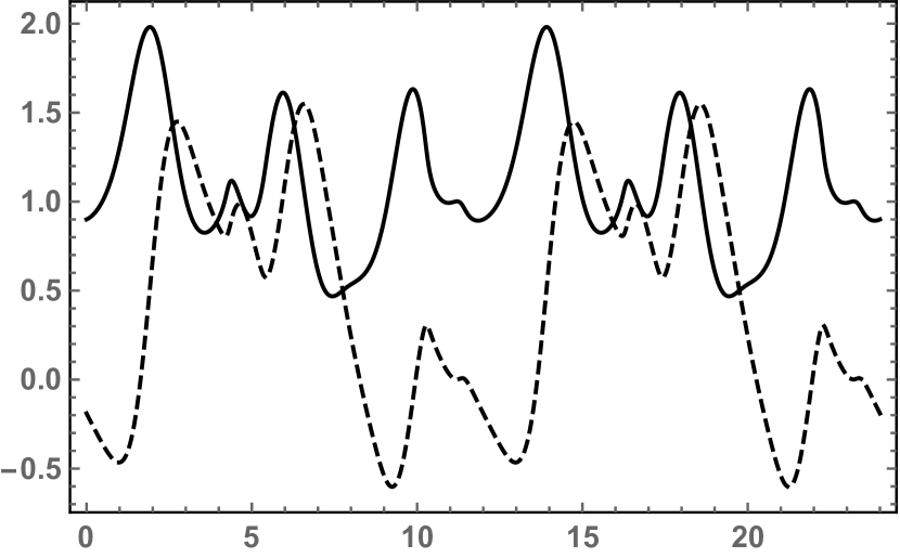
Figure 1: Initial value problem (43), (46), (47). Graphs of the real (bold curve) and imaginary (dashed curve) parts of the coordinate $x_{1}(t)$; period $12$.

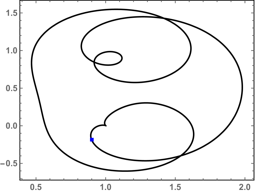
Figure 2: Initial value problem (43), (46), (47). Trajectory, in the complex $x$-plane, of $x_{1}(t)$; period $12$. The square indicates the initial condition $x_{1}(0)=0.90-0.19\,\mathbf{i}$.

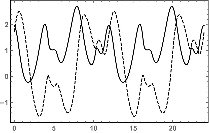
Figure 3: Initial value problem (43), (46), (47). Graphs of the real (bold curve) and imaginary (dashed curve) parts of the coordinate $x_{2}(t)$; period $12$.

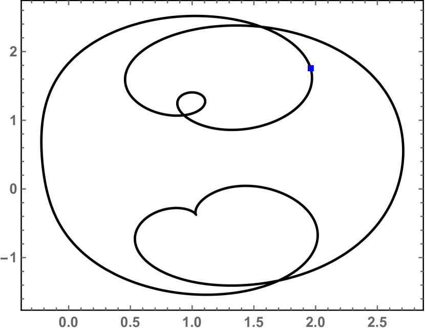
Figure 4: Initial value problem (43), (46), (47). Trajectory, in the complex $x$-plane, of $x_{2}(t)$; period $12$. The square indicates the initial condition $x_{2}(0)=1.96+1.75\,\mathbf{i}$.

Remark 3.1.2. The reader who wonders why the period of the solution of the initial value problem (43), (46), (47) is $12$ rather than $6$ is advised to read Ref. [18]. $\blacksquare$

Remark 3.1.3. Equations of motion (43), (44), (45) drastically simplify in the special case with $r_{1}=r_{2}=r_{3}=r,$ when they read

$$\ddot{x}_{1}=\left(x_{1}-x_{2}\right)^{-1}~{}\dot{x}_{1}~{}\left(\dot{x}_{1}+2~{}\dot{x}_{2}\right)+\mathbf{i}~{}\omega~{}r~{}\dot{x}_{1}~{},$$

$$\ddot{x}_{2}=-2~{}\left(x_{1}-x_{2}\right)^{-1}~{}\dot{x}_{1}~{}\left(\dot{x}_{1}+2~{}\dot{x}_{2}\right)+\mathbf{i}~{}\omega~{}r~{}\dot{x}_{2}~{};$$ (48)

$$\ddot{x}_{1}=\left[x_{1}~{}\left(x_{1}-x_{2}\right)\right]^{-1}~{}\dot{x}_{1}~{}\left(\dot{x}_{1}~{}x_{2}+2~{}\dot{x}_{2}~{}x_{1}\right)+\mathbf{i}~{}\omega~{}r~{}\dot{x}_{1}~{},$$

$$\ddot{x}_{2}=-2~{}\left[x_{1}~{}\left(x_{1}-x_{2}\right)\right]^{-1}~{}\dot{x}_{1}~{}\left(\dot{x}_{1}~{}x_{2}+2~{}\dot{x}_{2}~{}x_{1}\right)+\mathbf{i}~{}\omega~{}r~{}\dot{x}_{2}~{};$$ (49)

$$\ddot{x}_{1}=-\left[x_{1}~{}\left(x_{1}-x_{2}\right)\right]^{-1}~{}\dot{x}_{1}~{}\left[\dot{x}_{1}~{}\left(x_{1}-2~{}x_{2}\right)-2~{}\dot{x}_{2}~{}x_{1}\right]+\mathbf{i}~{}\omega~{}r~{}\dot{x}_{1}~{},$$

$$\ddot{x}_{2}=-2~{}\left[x_{1}^{2}~{}\left(x_{1}-x_{2}\right)\right]^{-1}~{}\dot{x}_{1}~{}\left[\dot{x}_{1}~{}x_{2}^{2}+2~{}\dot{x}_{2}~{}x_{1}^{2}\right]+\mathbf{i}~{}\omega~{}r~{}\dot{x}_{2}~{}.$$ (50)

$\blacksquare$

3.2 Example 3.2

In this example, we consider solvable $2$-body problems generated by the following $3$ models:

$$\text{{Model 3.2.1}: }\ddot{y}_{1}=-r_{1}^{2}~{}\omega^{2}~{}{y}_{1},~{}~{}~{}\ddot{y}_{2}=-r_{2}^{2}~{}\omega^{2}~{}{y}_{2}~{};$$ (51)

$$\text{{Model 3.2.2}: }\ddot{y}_{1}=-r_{1}^{2}~{}\omega^{2}~{}{y}_{1},~{}~{}~{}\ddot{y}_{3}=-r_{3}^{2}~{}\omega^{2}~{}{y}_{3}~{};$$ (52)

$$\text{{Model 3.2.3}: }\ddot{y}_{2}=-r_{2}^{2}~{}\omega^{2}~{}{y}_{2},~{}~{}~{}\ddot{y}_{3}=-r_{3}^{2}~{}\omega^{2}~{}{y}_{3}~{}.$$ (53)

Similarly to Example 1, $\omega$ is an arbitrary nonvanishing real number; and $r_{1},~{}r_{2},r_{3}$ are $3$ arbitrary nonvanishing rational numbers. These 3 models are Hamiltonian and integrable and their solutions

$$y_{m}\left(t\right)=y_{m}\left(0\right)\cos(r_{m}~{}\omega~{}t)+\frac{1}{r\omega}\dot{y}_{m}\left(0\right)~{}\sin(r_{m}~{}\omega~{}t)~{},~{}~{}~{}m=1,2,3~{},$$ (54)

are isochronous with a period which is an integer multiple of the basic period (42).

Remark 3.2.1. The last three systems are Hamiltonian because for every complex $\alpha$, the equation $\ddot{y}=\alpha~{}{y}$ is produced by the Hamiltonian $H(y,p)=p^{2}/2-\alpha~{}y^{2}/2$. $\blacksquare$

The following two-body problems are generated by the method described in Subsection 2.1, see (11), (12) and (13):

System 3.2.1:

$$\ddot{x}_{1}=\frac{\omega^{2}x_{1}\left[(-4r_{1}^{2}+r_{2}^{2})x_{1}+2(-r_{1}^{2}+r_{2}^{2})x_{2}\right]+2\dot{x}_{1}(\dot{x}_{1}+2\dot{x}_{2})}{2(x_{1}-x_{2})},$$

$$\ddot{x}_{2}=\frac{\omega^{2}x_{1}\left[(2r_{1}^{2}-r_{2}^{2})x_{1}+(3r_{1}^{2}-2r_{2}^{2})x_{2}\right]+r_{1}^{2}\omega^{2}x_{2}^{2}+2\dot{x}_{1}(\dot{x}_{1}+2\dot{x}_{2})}{(x_{1}-x_{2})}.$$ (55)

System 3.2.2:

$$\ddot{x}_{1}=\frac{\omega^{2}x_{1}^{2}\left[-2r_{1}^{2}x_{1}+(-r_{1}^{2}+r_{3}^{2})x_{2}\right]+2\dot{x}_{1}(x_{2}\dot{x}_{1}+2x_{1}\dot{x}_{2})}{2x_{1}(x_{1}-x_{2})},$$

$$\ddot{x}_{2}=\frac{\omega^{2}x_{1}x_{2}\left[r_{3}^{2}x_{1}-r_{1}^{2}(2x_{1}+x_{2})\right]+2\dot{x}_{1}(x_{2}\dot{x}_{1}+2x_{1}\dot{x}_{2})}{x_{1}(x_{1}-x_{2})}.$$ (56)

System 3.2.3:

$$\ddot{x}_{1}=\frac{\omega^{2}x_{1}^{2}\left[-r_{2}^{2}x_{1}+2(-r_{2}^{2}+r_{3}^{2})x_{2}\right]+2\dot{x}_{1}\left[2x_{2}\dot{x}_{1}-x_{1}(\dot{x}_{1}-2\dot{x}_{2})\right]}{2x_{1}(x_{1}-x_{2})},$$

$$\ddot{x}_{2}=\frac{\omega^{2}x_{1}^{2}x_{2}\left[(r_{2}^{2}-r_{3}^{2})x_{1}+(2r_{2}^{2}-r_{3}^{2})x_{2}\right]-2\dot{x}_{1}\left[x_{2}^{2}\dot{x}_{1}+2x_{1}^{2}\dot{x}_{2}\right]}{x_{1}^{2}(x_{1}-x_{2})}.$$ (57)

These 3 systems are Hamiltonian, solvable by algebraic operations and their solutions are isochronous.

Below we provide the plots of the solutions of system (55) with the parameters

$$r_{1}=\frac{1}{2},\;\;r_{2}=\frac{1}{3},\;\;\omega=2\pi,$$ (58)

satisfying the initial conditions

$$x_{1}(0)=-2.4-1.21\,\mathbf{i},\;\;x_{1}^{\prime}(0)=-6.82-3.92\,\mathbf{i},$$

$$x_{2}(0)=4.89+2.42\,\mathbf{i},\;\;x_{2}^{\prime}(0)=-6.81-2.44\,\mathbf{i}.$$ (59)

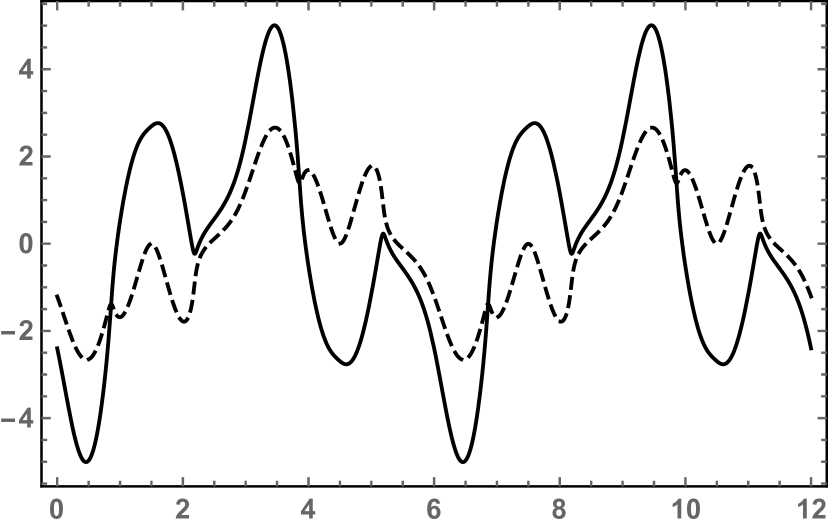
Figure 5: Initial value problem (55), (58), (59). Graphs of the real (bold curve) and imaginary (dashed curve) parts of the coordinate $x_{1}(t)$; period $6$.

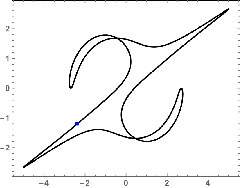
Figure 6: Initial value problem (55), (58), (59). Trajectory, in the complex $x$-plane, of $x_{1}(t)$; period $6$. The square indicates the initial condition $x_{1}(0)=-2.4-1.21\,\mathbf{i}$.

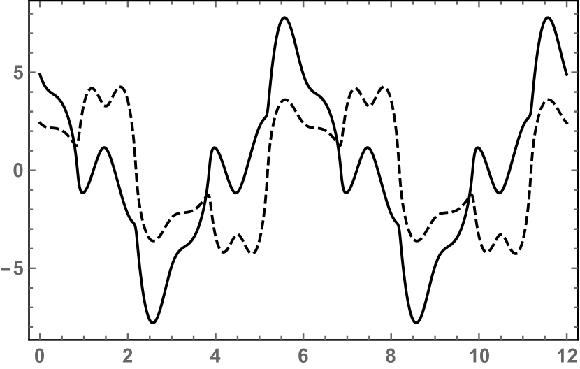
Figure 7: Initial value problem (55), (58), (59). Graphs of the real (bold curve) and imaginary (dashed curve) parts of the coordinate $x_{2}(t)$; period $6$.

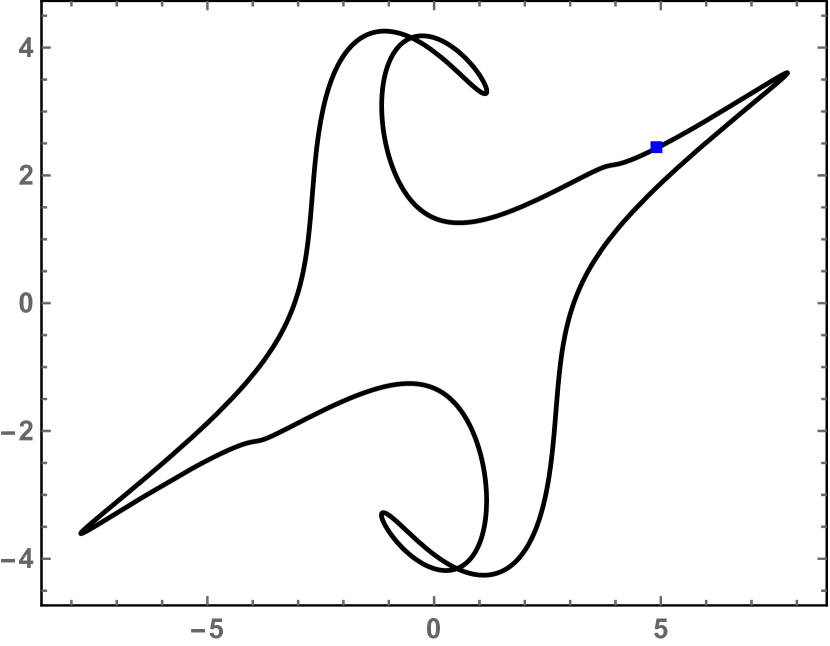
Figure 8: Initial value problem (55), (58), (59). Trajectory, in the complex $x$-plane, of $x_{2}(t)$; period $6$. The square indicates the initial condition $x_{2}(0)=4.89+2.42\,\mathbf{i}$.

Remark 3.2.2. Equations of motion (55), (56), (57) simplify significantly in the special case where $r_{1}=r_{2}=r_{3}=r$:

$$\ddot{x}_{1}=\left[2(x_{1}-x_{2})\right]^{-1}\left[-3\omega^{2}r^{2}x_{1}^{2}+2\dot{x}_{1}(\dot{x}_{1}+2\dot{x}_{2})\right],$$

$$\ddot{x}_{2}=(x_{1}-x_{2})^{-1}\left[\omega^{2}r^{2}(x_{1}^{2}+x_{1}x_{2}+x_{2}^{2})+2\dot{x}_{1}(\dot{x}_{1}+2\dot{x}_{2})\right];$$ (60)

$$\ddot{x}_{1}=\left[2x_{1}(x_{1}-x_{2})\right]^{-1}\left[-2\omega^{2}r^{2}x_{1}^{3}+2\dot{x}_{1}(x_{2}\dot{x}_{1}+2x_{1}\dot{x}_{2})\right],$$

$$\ddot{x}_{2}=\left[x_{1}(x_{1}-x_{2})\right]^{-1}\left[\omega^{2}r^{2}x_{1}x_{2}(x_{2}-x_{1})+2\dot{x}_{1}(x_{2}\dot{x}_{1}+2x_{1}\dot{x}_{2})\right];$$ (61)

$$\ddot{x}_{1}=\left[2x_{1}(x_{1}-x_{2})\right]^{-1}\left[-\omega^{2}r^{2}x_{1}^{3}+2\dot{x}_{1}(2x_{2}\dot{x}_{1}-x_{1}\dot{x}_{1}+2x_{1}\dot{x}_{2})\right],$$

$$\ddot{x}_{2}=\left[x_{1}^{2}(x_{1}-x_{2})\right]^{-1}\left[\omega^{2}r^{2}x_{1}^{2}x_{2}^{2}-2\dot{x}_{1}(x_{2}^{2}\dot{x}_{1}+2x_{1}^{2}\dot{x}_{2})\right].$$ (62)

$\blacksquare$

3.3 Example 3.3

In this example, we generate solvable $3$-body systems from the following $3$ models:

$$\text{{Model 3.3.1}: }\ddot{y}_{1}=-r_{1}^{2}~{}\omega^{2}~{}{y}_{1},~{}~{}~{}\ddot{y}_{2}=\mathbf{i}~{}r_{2}~{}\omega~{}\dot{y}_{2}~{};$$ (63)

$$\text{{Model 3.3.2}: }\ddot{y}_{1}=-r_{1}^{2}~{}\omega^{2}~{}{y}_{1},~{}~{}~{}\ddot{y}_{3}=\mathbf{i}~{}r_{3}~{}\omega~{}\dot{y}_{3}~{};$$ (64)

$$\text{{Model 3.3.3}: }\ddot{y}_{2}=-r_{2}^{2}~{}\omega^{2}~{}{y}_{2},~{}~{}~{}\ddot{y}_{3}=\mathbf{i}~{}r_{3}~{}\omega~{}\dot{y}_{3}~{}.$$ (65)

As in the previous Examples 3.1 and 3.2, $\omega$ is an arbitrary nonvanishing real number and $r_{1},~{}r_{2},r_{3}$ are $3$ arbitrary nonvanishing rational numbers. These 3 models are Hamiltonian (see Remarks 3.1.1 and 3.2.1) and integrable and their solutions are given by appropriate combinations of 2 formulas chosen from among the 6 formulas (41) and (54). For example, the solution of Model 3.3.1 is given by (54) with $m=1$ and (41) with $m=2$. These models are all isochronous with a period which is an integer multiple of the basic period (42).

These generating models yield the following solvable two-body problems, via the method described in Subsection 2.1, see (11), (12) and (13):

System 3.3.1:

$$\ddot{x}_{1} = \frac{1}{x_{1}-x_{2}}\Big{\{}\dot{x}_{1}(\dot{x}_{1}+2\,\dot{x}_{2})-(r_{1})^{2}\,\omega^{2}\,x_{1}\,(2\,x_{1}+x_{2})$$

$$-\mathbf{i}\,r_{2}\,\omega\,\left[\dot{x}_{1}\,(x_{1}+x_{2})+\dot{x}_{2}\,x_{1}\right]\Big{\}},$$

$$\ddot{x}_{2} = \frac{1}{x_{1}-x_{2}}\Big{\{}-2\,\dot{x}_{1}\,(\dot{x}_{1}+2\,\dot{x}_{2})+(r_{1})^{2}\,\omega^{2}\,(x_{1}+x_{2})\,(2\,x_{1}+x_{2})$$ (66)

$$+2\,\mathbf{i}\,r_{2}\,\omega\left[\dot{x}_{1}\,(x_{1}+x_{2})+\dot{x}_{2}\,x_{1}\right]\Big{\}}.$$

System 3.3.2:

$$\ddot{x}_{1} = \left[2\,x_{1}\,(x_{1}-x_{2})\right]^{-1}\Big{\{}2\,\dot{x}_{1}\,(\dot{x}_{1}\,x_{2}+2\,\dot{x}_{2}\,x_{1})-(r_{1})^{2}\,\omega^{2}\,x_{1}^{2}\,(2\,x_{1}+x_{2})$$

$$-\mathbf{i}\,r_{3}\,\omega\,x_{1}\,(2\,\dot{x}_{1}\,x_{2}+\dot{x}_{2}\,x_{1})\Big{\}}$$

$$\ddot{x}_{2} = \left[x_{1}\,(x_{1}-x_{2})\right]^{-1}\Big{\{}-2\,\dot{x}_{1}\,(\dot{x}_{1}\,x_{2}+2\,\dot{x}_{2}\,x_{1})+(r_{1})^{2}\,\omega^{2}\,x_{1}\,x_{2}\,(2\,x_{1}+x_{2})$$ (67)

$$+\mathbf{i}\,r_{3}\,\omega\,x_{1}\,(2\,\dot{x}_{1}\,x_{2}+\dot{x}_{2}\,x_{1})\Big{\}}$$

System 3.3.3:

$$\ddot{x}_{1} = -\left[2\,x_{1}\,(x_{1}-x_{2})\right]^{-1}\Big{\{}2\,\dot{x}_{1}\,\left[\dot{x}_{1}\,(x_{1}-2\,x_{2})-2\,\dot{x}_{2}\,x_{1}\right]+(r_{2})^{2}\,\omega^{2}\,(x_{1})^{2}\,(x_{1}+2\,x_{2})$$

$$+2\,\mathbf{i}\,r_{3}\,\omega\,x_{1}\,(2\,\dot{x}_{1}\,x_{2}+\dot{x}_{2}\,x_{1})\Big{\}},$$

$$\ddot{x}_{2} = \left[(x_{1})^{2}\,(x_{1}-x_{2})\right]^{-1}\Big{\{}-2\,\dot{x}_{1}\,\left[\dot{x}_{1}\,(x_{2})^{2}+2\,\dot{x}_{2}\,(x_{1})^{2}\right]+(r_{2})^{2}\,\omega^{2}\,(x_{1})^{2}\,x_{2}\,(x_{1}+2\,x_{2})$$ (68)

$$+\mathbf{i}\,r_{3}\,\omega\,x_{1}\,(x_{1}+x_{2})\,(2\,\dot{x}_{1}\,x_{2}+\dot{x}_{2}\,x_{1})\Big{\}}.$$

These 3 systems are Hamiltonian, solvable by algebraic operations and their solutions are isochronous.

Below we display the plots of the solutions of system (68) with the parameters

$$r_{2}=\frac{1}{3},\;\;r_{3}=\frac{1}{2},\;\;\omega=2\pi,$$ (69)

satisfying the initial conditions

$$x_{1}(0)=0.94-0.28\,\mathbf{i},\;\;\dot{x}_{1}(0)=-0.38-4.68\,\mathbf{i},$$

$$x_{2}(0)=1.40+1.11\,\mathbf{i},\;\;\dot{x}_{2}(0)=-9.20+2.50\,\mathbf{i}.$$ (70)

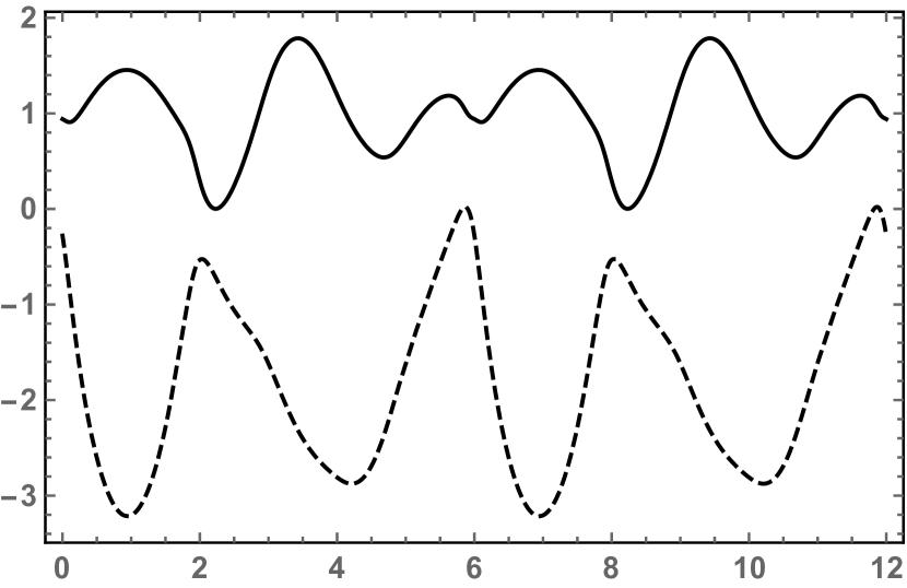
Figure 9: Initial value problem (68), (69), (70). Graphs of the real (bold curve) and imaginary (dashed curve) parts of the coordinate $x_{1}(t)$; period $6$.

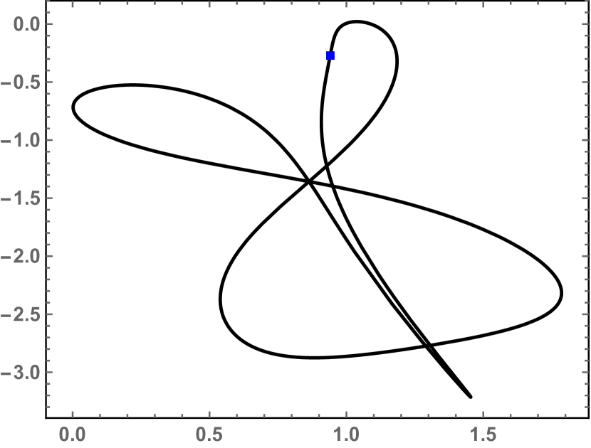
Figure 10: Initial value problem (68), (69), (70). Trajectory, in the complex $x$-plane, of $x_{1}(t)$; period $6$. The square indicates the initial condition $x_{1}(0)=0.94-0.28\,\mathbf{i}$.

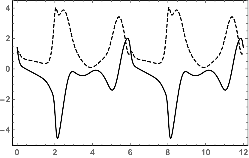
Figure 11: Initial value problem (68), (69), (70). Graphs of the real (bold curve) and imaginary (dashed curve) parts of the coordinate $x_{2}(t)$; period $6$.

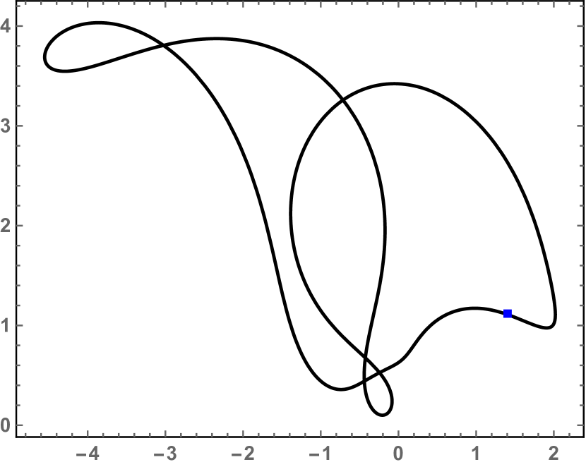
Figure 12: Initial value problem (68), (69), (70). Trajectory, in the complex $x$-plane, of $x_{2}(t)$; period $6$. The square indicates the initial condition $x_{2}(0)=1.40+1.11\,\mathbf{i}$.

3.4 Example 3.4

In this example, we consider the following $3$ generating models:

$$\text{{Model 3.4.1}: }\ddot{y}_{1}=-r^{2}~{}\omega^{2}~{}{y}_{1},~{}~{}~{}\ddot{y}_{2}=-a~{}\dot{y}_{2}~{};$$ (71)

$$\text{{Model 3.4.2}: }\ddot{y}_{1}=-r^{2}~{}\omega^{2}~{}{y}_{1},~{}~{}~{}\ddot{y}_{3}=-a~{}\dot{y}_{3}~{};$$ (72)

$$\text{{Model 3.4.3}: }\ddot{y}_{2}=-r^{2}~{}\omega^{2}~{}{y}_{2},~{}~{}~{}\ddot{y}_{3}=-a~{}\dot{y}_{3}~{}.$$ (73)

Here $a$ is a positive real number and $r$ is a nonvanishing rational number. These 3 models are Hamiltonian (see Remarks 3.1.1 and 3.2.1) and integrable and their solutions are given by appropriate selections from formulas (54) and

$$y_{m}(t)=y_{m}(0)+\frac{1}{a}\dot{y}_{m}(0)\left[1-\exp(-at)\right].$$ (74)

For example, the solution of Model 3.4.1 is given by (54) with $m=1$ and (74) with $m=2$. These models are all asymptotically isochronous [19].

These generating models yield the following solvable two-body problems, via the method described in Subsection 2.1, see (11), (12) and (13):

System 3.4.1:

$$\ddot{x}_{1} = (x_{1}-x_{2})^{-1}\Big{\{}\dot{x}_{1}\,(\dot{x}_{1}+2\,\dot{x}_{2})-r^{2}\,\omega^{2}\,x_{1}\,(2\,x_{1}+x_{2})$$

$$+a\,\left[\dot{x}_{1}\,(x_{1}+x_{2})+\dot{x}_{2}\,x_{1}\right]\Big{\}},$$

$$\ddot{x}_{2} = (x_{1}-x_{2})^{-1}\Big{\{}2\,\dot{x}_{1}(\dot{x}_{1}+2\,\dot{x}_{2})+r^{2}\,\omega^{2}\,(x_{1}+x_{2})\,(2\,x_{1}+x_{2})$$ (75)

$$-2\,a\,\left[\dot{x}_{1}\,(x_{1}+x_{2})+\dot{x}_{2}\,x_{1}\right]\Big{\}}.$$

System 3.4.2:

$$\ddot{x}_{1} = \left[2\,x_{1}\,(x_{1}-x_{2})\right]^{-1}\Big{\{}2\,\dot{x}_{1}\,(\dot{x}_{1}\,x_{2}+2\,\dot{x}_{2}\,x_{1})-r^{2}\,\omega^{2}\,(x_{1})^{2}\,(2\,x_{1}+x_{2})$$

$$+a\,x_{1}\,(2\,\dot{x}_{1}\,x_{2}+\dot{x}_{2}\,x_{1})\Big{\}},$$

$$\ddot{x}_{2} = \left[x_{1}\,(x_{1}-x_{2})\right]^{-1}\Big{\{}-2\,\dot{x}_{1}\,(\dot{x}_{1}\,x_{2}+2\,\dot{x}_{2}\,x_{1})+r\,\omega^{2}\,x_{1}\,x_{2}(2\,x_{1}+x_{2})$$ (76)

$$-a\,x_{1}\,(2\,\dot{x}_{1}\,x_{2}+\dot{x}_{2}\,x_{1})\Big{\}}.$$

System 3.4.3:

$$\ddot{x}_{1} = \left[2\,x_{1}\,(x_{1}-x_{2})\right]^{-1}\Big{\{}-2\,\dot{x}_{1}\,\left[\dot{x}_{1}\,(x_{1}-2\,x_{2})-2\,\dot{x}_{2}\,x_{1}\right]$$

$$-r^{2}\,\omega^{2}\,(x_{1})^{2}\,(x_{1}+2\,x_{2})+2\,a\,x_{1}\,(2\,\dot{x}_{1}\,x_{2}+\dot{x}_{2}\,x_{1})\Big{\}},$$

$$\ddot{x}_{2} = \left[(x_{1})^{2}\,(x_{1}-x_{2})\right]^{-1}\Big{\{}-2\,\dot{x}_{1}\,\left[\dot{x}_{1}\,(x_{2})^{2}+2\,\dot{x}_{2}(x_{1})^{2}\right]$$ (77)

$$+r^{2}\,\omega^{2}\,(x_{1})^{2}\,x_{2}\,(x_{1}+2\,x_{2})-a\,x_{1}\,(x_{1}+x_{2})(2\,\dot{x}_{1}\,x_{2}+\dot{x}_{2}\,x_{1})\Big{\}}.$$

These 3 systems are Hamiltonian, solvable by algebraic operations and their solutions are asymptotically isochronous.

Below we display the plots of the solutions of system (76) with the parameters

$$r=\frac{1}{3},\;\;\omega=2\pi,\;\;a=0.1,$$ (78)

satisfying the initial conditions

$$x_{1}(0)=1.21,\;\;\dot{x}_{1}(0)=-0.56-2.34\,\mathbf{i},$$

$$x_{2}(0)=1.42+0.89\,\mathbf{i},\;\;\dot{x}_{2}(0)=-1.78-0.54\,\mathbf{i}.$$ (79)

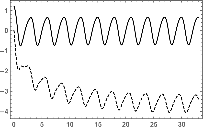
Figure 13: Initial value problem (76), (78), (79). Graphs of the real (bold curve) and imaginary (dashed curve) parts of the coordinate $x_{1}(t)$.

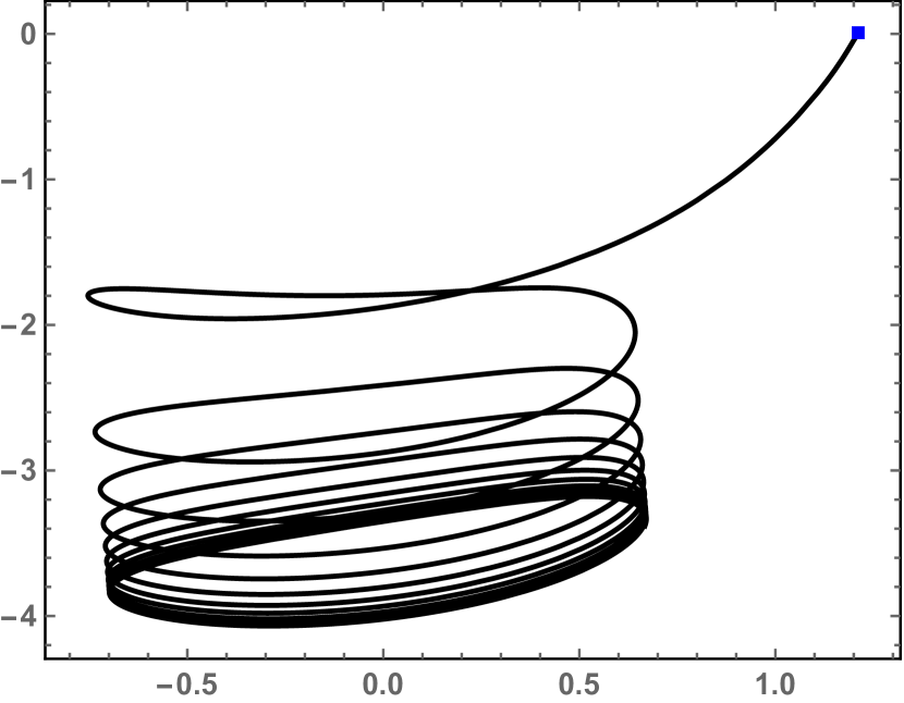
Figure 14: Initial value problem (76), (78), (79). Trajectory, in the complex $x$-plane, of $x_{1}(t)$. The square indicates the initial condition $x_{1}(0)=1.21$.

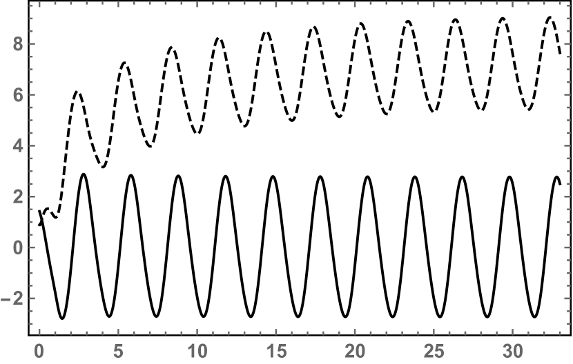
Figure 15: Initial value problem (76), (78), (79). Graphs of the real (bold curve) and imaginary (dashed curve) parts of the coordinate $x_{2}(t)$.

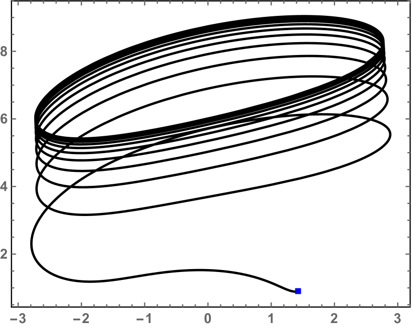
Figure 16: Initial value problem (76), (78), (79). Trajectory, in the complex $x$-plane, of $x_{2}(t)$. The square indicates the initial condition $x_{2}(0)=1.42+0.89\,\mathbf{i}$.

3.5 Example 3.5

In this example, we take as a starting point of our treatment one of the following $4$ generating models:

$$\text{{Model 3.5.1}: }\ddot{y}_{1}=-r_{1}^{2}~{}\omega^{2}~{}{y}_{1},~{}~{}~{}\ddot{y}_{2}=-r_{2}^{2}~{}\omega^{2}~{}{y}_{2},~{}~{}~{}\ddot{y}_{3}=-r_{3}^{2}~{}\omega^{2}~{}{y}_{3}~{};$$ (80)

$$\text{{Model 3.5.2}: }\ddot{y}_{1}=-r_{1}^{2}~{}\omega^{2}~{}{y}_{1},~{}~{}~{}\ddot{y}_{2}=-r_{2}^{2}~{}\omega^{2}~{}{y}_{2},~{}~{}~{}\ddot{y}_{4}=-r_{4}^{2}~{}\omega^{2}~{}{y}_{4}~{};$$ (81)

$$\text{{Model 3.5.3}: }\ddot{y}_{1}=-r_{1}^{2}~{}\omega^{2}~{}{y}_{1},~{}~{}~{}\ddot{y}_{3}=-r_{3}^{2}~{}\omega^{2}~{}{y}_{3},~{}~{}~{}\ddot{y}_{4}=-r_{4}^{2}~{}\omega^{2}~{}{y}_{4}~{};$$ (82)

$$\text{{Model 3.5.4}: }\ddot{y}_{2}=-r_{2}^{2}~{}\omega^{2}~{}{y}_{2},~{}~{}~{}\ddot{y}_{3}=-r_{3}^{2}~{}\omega^{2}~{}{y}_{3},~{}~{}~{}\ddot{y}_{4}=-r_{4}^{2}~{}\omega^{2}~{}{y}_{4}~{}.$$ (83)

Similarly to Example 1, $\omega$ is an arbitrary nonvanishing real number and $r_{1},~{}r_{2},~{}r_{3},~{}r_{4}$ are $4$ arbitrary nonvanishing rational numbers. These 4 models are Hamiltonian (see Remark 3.2.1) and integrable and their solutions (see (54) with $m=1,2,3,4$) are isochronous with a period which is an integer multiple of the basic period (42).

These generating models yield the following four solvable three-body problems, via the method described in Subsection 2.2, see (32). More precisely, each Model 5.(${5-\bar{m}}$) generates

System 3.5.($\mathbf{5-\bar{m}}$), where $\mathbf{\bar{m}\in\{1,2,3,4\}}$:

$$\ddot{x}_{1} = -(4-\bar{m})\frac{(\dot{x}_{1})^{2}}{x_{1}}+\frac{\dot{x}_{1}(2\,\dot{x}_{2}+\dot{x}_{1})}{x_{1}-x_{2}}+\frac{\dot{x}_{1}(2\,\dot{x}_{3}+\dot{x}_{1})}{x_{1}-x_{3}}$$

$$-\frac{1}{2\,(x_{1}-x_{2})\,(x_{1}-x_{3})}\sum_{m=1,m\neq\bar{m}}^{4}\,(m-\bar{m})\,(r_{m})^{2}\,\omega^{2}(\,x_{1})^{3-m}\,y_{m},$$

$$\ddot{x}_{2} = \frac{2\,\dot{x}_{2}\,\dot{x}_{3}}{x_{2}-x_{3}}+\frac{2\,\dot{x}_{1}}{x_{2}-x_{1}}\,\Big{[}2\,\dot{x}_{2}+\left(\frac{x_{2}}{x_{1}}\right)^{4-\bar{m}}\,\left(\frac{x_{1}-x_{3}}{x_{2}-x_{3}}\right)\,\dot{x}_{1}\Big{]}$$

$$+\frac{(x_{2})^{4-\bar{m}}}{(x_{2}-x_{1})\,(x_{2}-x_{3})}\sum_{m=1,m\neq\bar{m}}^{4}\,(r_{m})^{2}\,\omega^{2}\,y_{m}\left[\frac{(x_{2})^{\bar{m}-m}-(x_{1})^{\bar{m}-m}}{x_{2}-x_{1}}\right],$$

$$\ddot{x}_{3} = -\frac{2\,\dot{x}_{2}\,\dot{x}_{3}}{x_{2}-x_{3}}+\frac{2\,\dot{x}_{1}}{x_{3}-x_{1}}\Big{[}2\,\dot{x}_{3}+\left(\frac{x_{3}}{x_{1}}\right)^{4-\bar{m}}\left(\frac{x_{1}-x_{2}}{x_{3}-x_{2}}\right)\dot{x}_{1}\Big{]}$$

$$+\frac{(x_{3})^{4-\bar{m}}}{(x_{3}-x_{1})\,(x_{3}-x_{2})}\sum_{m=1,m\neq\bar{m}}^{4}\,(r_{m})^{2}\,\omega^{2}\,y_{m}\left[\frac{(x_{3})^{\bar{m}-m}-(x_{1})^{\bar{m}-m}}{x_{3}-x_{1}}\right],$$

where

$$y_{1}=-(2\,x_{1}+x_{2}+x_{3}),$$

$$y_{2}=(x_{1})^{2}+2\,x_{1}\,x_{2}+2\,x_{1}\,x_{3}+x_{2}\,x_{3},$$

$$y_{3}=-\left[(x_{1})^{2}\,x_{2}+(x_{1})^{2}\,x_{3}+2\,x_{1}\,x_{2}\,x_{3}\right],$$

$$y_{4}=(x_{1})^{2}\,x_{2}\,x_{3},$$ (84b)

see (23). These 4 systems are Hamiltonian, solvable by algebraic operations and their solutions are isochronous.

Below we display the plots of the solutions of system (84) for the case

$$\bar{m}=3$$ (85)

with the parameters

$$r_{1}=\frac{1}{2},~{}r_{2}=\frac{1}{3},~{}r_{4}=\frac{2}{3};\;\;\omega=2\pi,$$ (86)

satisfying the initial conditions

$$x_{1}(0)=1.74+1.42\,\mathbf{i},\;\;\dot{x}_{1}(0)=12.47+4.46\,\mathbf{i},$$

$$x_{2}(0)=-3.20+0.52\,\mathbf{i},\;\;\dot{x}_{2}(0)=-10.23+6.40\,\mathbf{i},$$

$$x_{3}(0)=0.44-3.15\,\mathbf{i},\;\;\dot{x}_{3}(0)=3.16-14.66\,\mathbf{i}.$$ (87)

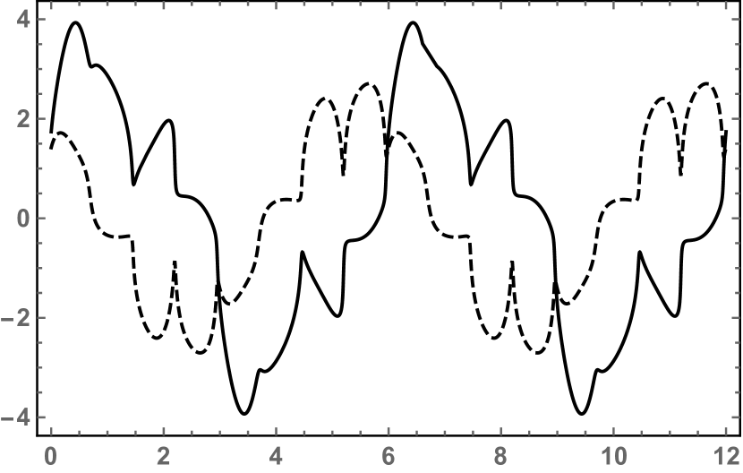
Figure 17: Initial value problem (84), (85), (86), (87). Graphs of the real (bold curve) and imaginary (dashed curve) parts of the coordinate $x_{1}(t)$; period 6.

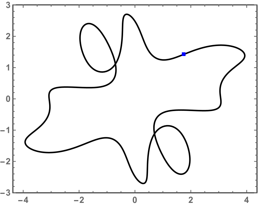
Figure 18: Initial value problem (84), (85), (86), (87). Trajectory, in the complex $x$-plane, of $x_{1}(t)$. The square indicates the initial condition $x_{1}(0)=1.74+1.42\,\mathbf{i}$.

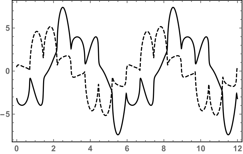
Figure 19: Initial value problem (84), (85), (86), (87). Graphs of the real (bold curve) and imaginary (dashed curve) parts of the coordinate $x_{2}(t)$; period 6.

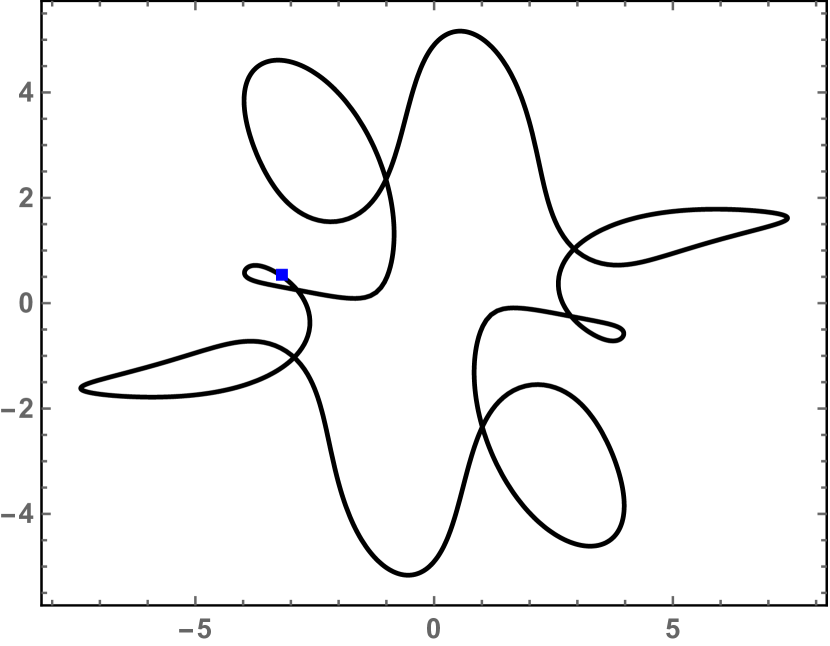
Figure 20: Initial value problem (84), (85), (86), (87). Trajectory, in the complex $x$-plane, of $x_{2}(t)$. The square indicates the initial condition $x_{2}(0)=-3.20+0.52\,\mathbf{i}$.

Figure 21: Initial value problem  (84), (85), (86), (87). Graphs of the real (bold curve) and imaginary (dashed curve) parts of the coordinate $x_{3}(t)$; period 6.

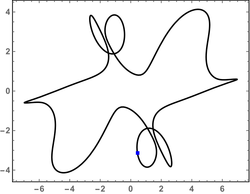
Figure 22: Initial value problem (84), (85), (86), (87). Trajectory, in the complex $x$-plane, of $x_{3}(t)$. The square indicates the initial condition $x_{3}(0)=0.44-3.15\,\mathbf{i}$.

4 Outlook

In this Section 4 we tersely outline further developments which are a natural continuation of the findings reported in this paper.

Two kinds of generalizations of the results reported in this paper are obvious goals. One—already mentioned at the end of the introductory part of Section 2—is to extend the results of this paper—which are confined to time-dependent polynomials of arbitrary degree in the complex variable $z$ featuring, for all time, a one double zero—to the most general case of analogous polynomials featuring, for all time, several zeros, each with an arbitrary (fixed) multiplicity. Another direction of generalization is to obtain formulas—say, analogous to (13) and (30)—expressing time-derivatives of order $k>2$ of the zeros $x_{n}\left(t\right)$ of such time-dependent polynomials.

And an unlimited area of additional study is of course open, consisting in the identification and investigation of new many-body problems in the plane amenable to exact treatments via techniques analogous to those demonstrated by the few examples treated above (see Section 3) and in previous publications [1]-[14]—including possible applications of these findings.

References

- [1] Calogero, F.: New solvable variants of the goldfish many-body problem. Studies Appl. Math. 137 (1), 123-139 (2016); DOI: 10.1111/sapm.12096.
- [2] Bihun, O., Calogero, F.: A new solvable many-body problem of goldfish type. J. Nonlinear Math. Phys. 23, 28-46 (2016).
- [3] Bihun, O. , Calogero, F.: Novel solvable many-body problems. J. Nonlinear Math. Phys. 23, 190-212 (2016).
- [4] Bihun, O., Calogero, F.: Generations of monic polynomials such that the coefficients of the polynomials of the next generation coincide with the zeros of polynomial of the current generation, and new solvable many-body problems. Lett. Math. Phys. 106 (7), 1011-1031 (2016).
- [5] Calogero, F.: A solvable -body problem of goldfish type featuring arbitrary coupling constants. J. Nonlinear Math. Phys. 23, 300-305 (2016).
- [6] Calogero, F.: Three new classes of solvable -body problems of goldfish type with many arbitrary coupling constants. Symmetry 8, 53 (2016).
- [7] Bruschi, M., Calogero, F.: A convenient expression of the time-derivative , of arbitrary order , of the zero of a time-dependent polynomial of arbitrary degree in , and solvable dynamical systems. J. Nonlinear Math. Phys. 23, 474-485 (2016).
- [8] Calogero, F.: Novel isochronous -body problems featuring arbitrary rational coupling constants. J. Math. Phys. 57, 072901 (2016); http://dx.doi.org/10.1063/1.4954851.
- [9] Calogero, F.: Yet another class of new solvable -body problems of goldfish type. Qualit. Theory Dyn. Syst. 16(3) 561-577 (2017); DOI: 10.1007/s12346-016-0215-y.
- [10] Calogero, F.: New solvable dynamical systems. J. Nonlinear Math. Phys. 23, 486-493 (2016).
- [11] Calogero, F.: Integrable Hamiltonian -body problems in the plane featuring arbitrary functions. J. Nonlinear Math. Phys. 24(1), 1-6 (2017).
- [12] Calogero, F.: New C-integrable and S-integrable systems of nonlinear partial differential equation. J. Nonlinear Math. Phys. 24(1), 142-148 (2017).
- [13] Bihun, O. , Calogero, F.: Generations of solvable discrete-time dynamical systems. J. Math. Phys. 58, 052701 (2017); doi: 10.1063/1.4928959.
- [14] Calogero, F.: Zeros of polynomials and solvable nonlinear evolution equations. Cambridge University Press, Cambridge, England, 2018 (in press).
- [15] Calogero, F.: Motion of Poles and Zeros of Special Solutions of Nonlinear and Linear Partial Differential Equations, and Related “Solvable” Many Body Problems. Nuovo Cimento 43B, 177-241 (1978).
- [16] Calogero, F.: Classical Many-Body Problems Amenable to Exact Treatments. Lecture Notes in Physics m66, Springer, Heidelberg, 2001 (750 pages).
- [17] Calogero, F.: Isochronous Systems. Oxford University Press, Oxford, England, 2008 (250 pages; marginally updated paperback version, 2012).
- [18] Gómez-Ullate, D. , Sommacal, M.: Periods of the goldfish many-body problem. J. Nonlinear Math. Phys. 12, Suppl. 1, 351-362 (2005).
- [19] Calogero, F., Gómez-Ullate, D.: Asymptotically isochronous systems. J. Nonlinear Math. Phys. 15, 410-426 (2008).