Unravelling the stereodynamics of cold HD-H₂ collisions

Abstract

Measuring inelastic rates with partial wave resolution requires temperatures close to a Kelvin or below, even for the lightest molecule. In a recent experiment Perreault et al. Perreault et al. (2018a) studied collisional relaxation of excited HD molecules in the $v=1,j=2$ state by para- and ortho-H₂ at a temperature of about 1 K, extracting the angular distribution of scattered HD in the $v=1,j=0$ state. By state-preparation of the HD molecules, control of the angular distribution of scattered HD was demonstrated. Here, we report a first-principles simulation of that experiment which enables us to attribute the main features of the observed angular distribution to a single $L=2$ partial-wave shape resonance. Our results demonstrate important stereodynamical insights that can be gained when numerically-exact quantum scattering calculations are combined with experimental results in the few-partial-wave regime.

I Introduction

The ultimate goal of chemistry is the complete quantum state control of both reactants and products. Understanding the state-to-state stereodynamics of collision processes is a perquisite for attaining such control Bernstein et al. (1987); Zare (1998); Aldegunde et al. (2005); Perreault et al. (2018a). Reducing the collision energy to a Kelvin or less simplifies collisional processes by restricting the relevant number of partial waves. Thanks to recent developments in molecule cooling and trapping Wynar et al. (2000); Regal et al. (2003); Sawyer et al. (2007); Shuman et al. (2010); Hummon et al. (2013); Akerman et al. (2017); Anderegg et al. (2017); Truppe et al. (2017) and merged beams Henson et al. (2012); Jankunas et al. (2014); Klein et al. (2017); Perreault et al. (2018b) it is now increasingly possible to study molecular systems in this few-partial-wave regime Ospelkaus et al. (2010); Knoop et al. (2010); Rui et al. (2017); Perreault et al. (2017); Wolf et al. (2017); van der Poel et al. (2018); Amarasinghe and Suits (2017).

The stereodynamics of many inelastic and reactive molecular encounters is strongly influenced by resonances, which occur via either tunneling through a centrifugal barrier (shape resonance) or coupling to a bound state of a closed channel (Fano-Feshbach resonance) Chandler (2010); Klein et al. (2017); Amarasinghe and Suits (2017); Bergeat et al. (2015). Low-energy collisions of light molecules such as H₂ in the region of 1 K occur in a “Goldilocks zone” – neither too hot nor too cold – where chemical processes are dominated by just a few partial waves. However, experimental studies of molecular collisions and measurements of product angular distributions in this regime have been a significant challenge, in particular for neutral molecules such as H₂ and HD which are not magnetically trappable and have zero or very small dipole moment (for HD).

In a landmark experiment, Perreault et al. reported four-vector correlations for collisions of excited HD molecules in the $v=1,j=2$ level with D₂ and H₂ at a collision energy around 1 K Perreault et al. (2017, 2018a). In the experiment HD and H₂/D₂ are co-expanded in a single beam, and the HD molecules are prepared in one of two specific well-defined states using Stark-induced adiabatic Raman passage (SARP). SARP combined with a co-expansion in a molecular beam therefore provides a powerful tool for studying the stereodynamics of cold collisions without having to explicitly remove their kinetic energy.

Here, we report a first-principles simulation of the experiment of Perreault et al. based on full-dimensional quantum scattering calculations. In doing so we unravel the stereodynamics of the collision process and attribute the observed experimental angular distribution to a $L=2$ shape resonance in the incoming channel. We also explain the origin of the symmetric angular distribution observed in the experiment.

II Methods

Being the simplest neutral molecule-molecule system, H₂+H₂/HD collisions are amenable to full-dimensional quantum scattering calculations Lin and Guo (2002); Pogrebnya and Clary (2002); Gatti et al. (2005); Quéméner et al. (2008) and high quality ab initio potential energy surfaces are available. In this work we have used the full-dimensional H₂-H₂ potential of Hinde Hinde (2008), which has been used extensively in recent years to study scattering of H₂ on H₂ and its isotopologs dos Santos et al. (2011); Balakrishnan et al. (2011). Its features compare well with the other available potentials for the H₂-H₂ system Boothroyd et al. (1991); Patkowski et al. (2008). In particular, its accuracy is comparable to the four-dimensional potential of Patkowski et al. Patkowski et al. (2008) which is considered to be the most accurate for the H₂-H₂ system (with an uncertainty of about 0.15 K or about 0.3% at the minimum of the potential well).

Scattering calculations for collisions of HD with H₂ were performed in full-dimensionality using a modified version of the TwoBC code Krems . The methodology is well established and outlined in detail Quéméner et al. (2008); Quéméner and Balakrishnan (2009); dos Santos et al. (2011), and has been applied to other similar systems Yang et al. (2015, 2018, 2016); dos Santos et al. (2013). Here we briefly review the methodology in order to define notation. The scattering calculations are performed within the time-independent close-coupling formalism yielding the usual asymptotic $S$ matrix Arthurs and Dalgarno (1960). For convenience, we label each asymptotic channel by the combined molecular state (CMS) $\alpha=v_{1}j_{1}v_{2}j_{2}$, where $v$ and $j$ are vibrational and rotational quantum numbers respectively and the subscript 1 refers to HD and 2 to H₂. The integral cross section for state-to-state rovibrationally inelastic scattering is given by,

$$\sigma_{\alpha\to\alpha^{\prime}}= \frac{\pi}{(2j_{1}+1)(2j_{2}+1)k_{\alpha}^{2}}$$

$$\times \sum_{J,j_{12},j^{\prime}_{12},l,l^{\prime}}(2J+1)|T^{J}_{\alpha lj_{12},\alpha^{\prime}l^{\prime}j^{\prime}_{12}}|^{2}.$$

where $k^{2}=2\mu E/\hbar^{2}$, $T^{J}=1-S^{J}$, $L$ is the orbital angular momentum, $J$ the total angular momentum (J = L + j₁₂), and j₁₂ = j₁ + j₂. To compute the differential cross sections relevant to this work we also need the scattering amplitude, which has previously been given by Schaefer et al.  Schaefer and Meyer (1979) in the helicity representation,

$$q=\frac{1}{2k_{\alpha}}\sum_{J} (2J+1) \sum_{j_{12},j^{\prime}_{12},l,l^{\prime}}i^{l-l^{\prime}+1}T^{J}_{\alpha lj_{12},\alpha^{\prime}l^{\prime}j^{\prime}_{12}}d^{J}_{m_{12},m^{\prime}_{12}}(\theta)$$

$$\times \big{\langle}j^{\prime}_{12}m^{\prime}_{12}J-m^{\prime}_{12}|l^{\prime}0\big{\rangle}\big{\langle}j_{12}m_{12}J-m_{12}|l0\big{\rangle}$$

$$\times \big{\langle}j^{\prime}_{1}m^{\prime}_{1}j^{\prime}_{2}m^{\prime}_{2}|j^{\prime}_{12}m^{\prime}_{12}\big{\rangle}\big{\langle}j_{1}m_{1}j_{2}m_{2}|j_{12}m_{12}\big{\rangle}$$

where $d^{J}_{m_{12},m^{\prime}_{12}}(\theta)$ is Wigner’s small $d$ rotation matrix. The rovibrational state-to-state differential cross section is then given by

$$\frac{d\sigma_{\alpha\to\alpha^{\prime}}}{d\Omega} =\frac{1}{(2j_{1}+1)(2j_{2}+1)}$$

$$\times \sum_{m_{1},m_{2},m_{12},m^{\prime}_{1},m^{\prime}_{2},m^{\prime}_{12}}|q_{\alpha,m_{1},m_{2},m_{12}\to\alpha^{\prime},m^{\prime}_{1},m^{\prime}_{2},m^{\prime}_{12}}|^{2}.$$

III Results

In the recent work of Perreault et al. collisions of HD($v=1,j=2$) with H₂($v=0,j=0,1$) were studied in the 0-10 K regime and the angular distribution of HD($v=1,j=0$) measured Perreault et al. (2018a). Figure 1 shows the corresponding theoretical integral cross section for, $\alpha=1200\to 1000$ and $\alpha=1201\to 1001$. It is clearly seen that there are shape resonances for collisions with both ortho-H₂ and para-H₂, in the vicinity of 1 K, with the dominant feature being a $L=2$ shape resonance with ortho-H₂ at around 1 K.

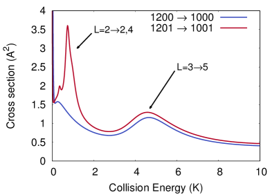
Figure 1: Integral state-to-state cross sections for HD($v=1,j=2$) $\to$ HD($v=1,j=0$) in collisions with H₂($j=0,1$)

In order to gain insight into the nature of the resonances seen in Fig. 1 we analyzed the effective potentials corresponding to different incoming partials waves $L$,

$$V^{J}(R) = \epsilon_{v_{1}j_{1}v_{2}j_{2}}$$

$$+ U^{J}_{v_{1}j_{1}v_{2}j_{2}Lj_{12},v^{\prime}_{1}j^{\prime}_{1}v^{\prime}_{2}j^{\prime}_{2}L^{\prime}j^{\prime}_{12}}(R)+\frac{L(L+1)\hbar^{2}}{2\mu R^{2}}.$$

The first term is the energy of the CMS obtained by adding the asymptotic rovibrational energies of HD and H₂. The second term is the diabatic potential energy coupling matrix and the third term is the centrifugal potential for the orbital angular momentum $L$. At large intermolecular separations, the energies of the different channels that correspond to the same CMS converge to its asymptotic value. The effective potential matrix is diagonalized at each value of $R$ and the eigenvalues as a function of $R$ correspond to a series of adiabatic potentials. Bound or quasibound states of these one-dimensional potentials correspond to HD-H₂ complexes, and the decay of the quasibound states leads to the resonances seen in Fig. 1. Figure 2 shows the potentials for $L=0,1,2,3,4$ for the asymptotic state 1201 along with the corresponding one-dimensional wavefunctions – shown at the bound or quasibound energies. It is the quasibound states at $\approx 1$ K and $\approx 5$ K in the $L=2$ and 3 channels respectively which lead to the shape resonances seen in Fig. 1. The corresponding outgoing dominant partial waves are $L^{\prime}=2$ and 4 for $L=2$ and $L^{\prime}=5$ for $L=3$ as shown in Fig. 1.

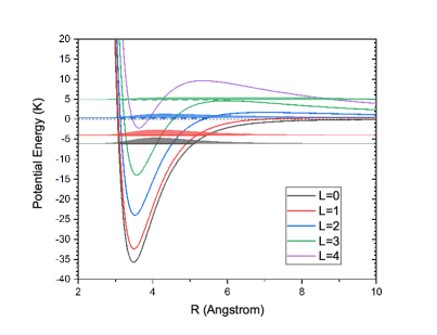
Figure 2: One-dimensional adiabatic potentials and wavefunctions of the HD-H₂ system as a function of $R$.

The experimental setup is described in detail in a series of papers by Perreault et al. Perreault et al. (2017, 2018b, 2018a). Here we only outline the details necessary for making a comparison with our theory results. In the experiment HD and H₂ are co-expanded in a single beam. The HD molecule is prepared in one of two specific states using the SARP technique. H-SARP prepares the HD($v_{1}=1,j_{1}=2$) in a state $|j_{1}=2,m_{1}=0\rangle$, where $m_{1}$ refers to the angular-momentum component along the relative velocity axis, in which case the HD bond is aligned parallel to the relative velocity. V-SARP, prepares the HD($v_{1}=1,j_{1}=2$) in a state

$$\sqrt{\frac{3}{8}}|j_{1}=2,m_{1}=-2\rangle - \frac{1}{2}|j_{1}=2,m_{1}=0\rangle$$

$$+ \sqrt{\frac{3}{8}}|j_{1}=2,m_{1}=2\rangle,$$

in which case the HD bond is aligned perpendicular to the relative velocity. The H and V in H-SARP and V-SARP refer to the horizontal and vertical orientations of the SARP laser relative to the beam velocity. The H₂ on the other hand is not state prepared and the ratio of para-H₂ to ortho-H₂ in the beam is taken to be 1 to 3. The experiment then measures the rate of HD($v_{1}=1,j_{1}=0$) scattered into a solid angle $\Omega$ relative to the beam velocity.

In order to compare with the experimental result we need to account for these experimental particulars. When molecules are prepared using H-SARP or V-SARP Eq. (II) for the differential cross-section has to be modified to account for the interference between the different $m$’s in the initial state preparation. For H-SARP it becomes

$$\frac{d\sigma^{H}_{\alpha\to\alpha^{\prime}}}{d\omega} = \frac{1}{(2j_{2}+1)}$$

$$\sum_{m_{12},m^{\prime}_{12},m_{1}^{\prime},m_{2},m^{\prime}_{2}}|q_{\alpha,m_{1}=0,m_{2},m_{12}\to\alpha^{\prime},m^{\prime}_{1},m^{\prime}_{2},m^{\prime}_{12}}|^{2},$$

while for V-SARP it becomes

$$\frac{d\sigma^{V}_{\alpha\to\alpha^{\prime}}}{d\omega}=\frac{1}{(2j_{2}+1)}$$ (7)

$$\sum_{m_{12},m^{\prime}_{12},m_{1}^{\prime},m_{2},m^{\prime}_{2}} | \sqrt{\frac{3}{8}}q_{\alpha,m_{1}=-2,m_{2},m_{12}\to\alpha^{\prime},m^{\prime}_{1},m^{\prime}_{2},m^{\prime}_{12}}$$

$$- \frac{1}{2}q_{\alpha,m_{1}=0,m_{2},m_{12}\to\alpha^{\prime},m^{\prime}_{1},m^{\prime}_{2},m^{\prime}_{12}}$$

$$+ \sqrt{\frac{3}{8}}q_{\alpha,m_{1}=+2,m_{2},m_{12}\to\alpha^{\prime},m^{\prime}_{1},m^{\prime}_{2},m^{\prime}_{12}}|^{2}.$$

As seen in Fig. 1 the dominant feature seen in the experiment is expected to be an $L=2$ shape resonance from collisions with ortho-H₂, especially when the relative population of ortho-H₂ and para-H₂ in the beam is taken into account. Figure 3 shows the differential rate (defined below) as a function of the relative velocity for the state-to-state transition, HD($v=1,j=2$) $\to$ HD($v=1,j=0$) in collisions with ortho-H₂ for H-SARP and V-SARP. The $L=2$ shape resonance seen in Fig. 1 is clearly visible at around 100 ms^-1 ($\approx$1 K). The initial alignment of the HD with respect to the beam velocity clearly makes a significant difference in the angular distribution. For V-SARP, where the HD bond axis is aligned perpendicular to the beam axis, the dominant scattering is at around 90 degrees whereas for H-SARP, where the HD bond axis is aligned parallel to the beam axis, there is also significant forward scattering at around 20 degrees. The equivalent figures for collisions with para-H₂ are given in the supplemental materials.

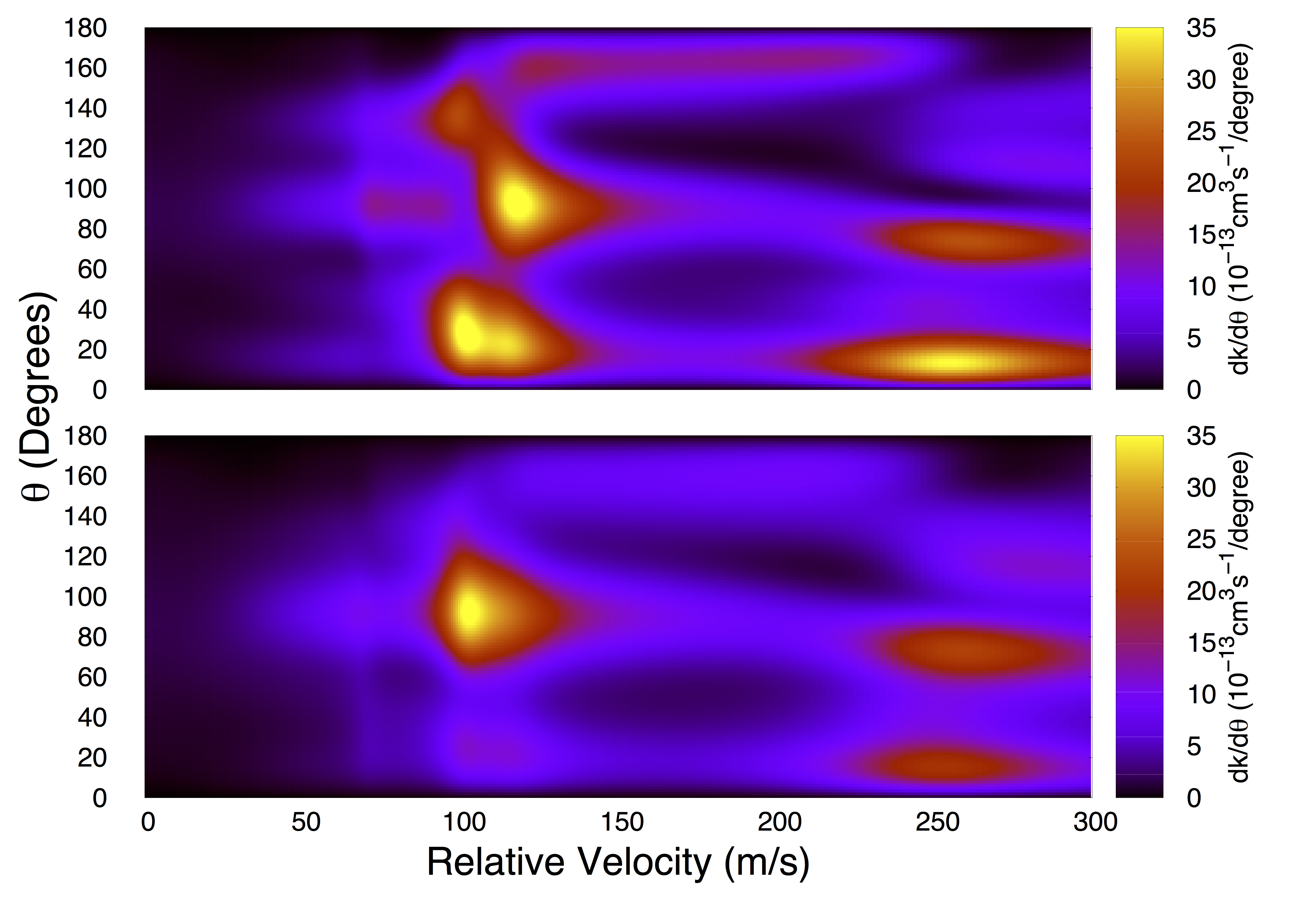
Figure 3: The differential state-to-state rate for the transition HD($v=1,j=2$) $\to$ HD($v=1,j=0$) in collisions with ortho-H₂ where the HD was prepared with H-SARP (upper panel) and V-SARP (lower panel).

In order to make an explicit comparison with the experimental angular distribution, we also have to average over both the relative velocity distribution and the relative populations of ortho-H₂ and para-H₂. The experimental velocity distributions for HD and H₂ are given by the Gaussian distributions $P(v_{\mathrm{HD}})\sim\mathcal{N}(\mu_{\mathrm{HD}}=2814,\sigma_{\mathrm{HD}}^{2}=71^{2}/2)$ and $P(v_{\mathrm{H}_{2}})\sim\mathcal{N}(\mu_{\mathrm{H}_{2}}=2740,\sigma_{\mathrm{H}_{2}}^{2}=105^{2}/2)$, where $v$, $\mu$, and $\sigma$ are in units of ms^-1 Perreault et al. (2018b). With the relative velocity defined as $v_{\mathrm{rel}}=v_{\mathrm{HD}}-v_{\mathrm{H}_{2}}$ the relative velocity distribution is then given by convolving the two distributions yielding $P(v_{\mathrm{rel}})\sim\mathcal{N}(\mu_{\mathrm{rel}}=\mu_{\mathrm{HD}}-\mu_{\mathrm{H}_{2}},\sigma_{\mathrm{rel}}^{2}=\sigma_{\mathrm{HD}}^{2}+\sigma_{\mathrm{H}_{2}}^{2}$). In the experiment the scattering angle $\theta_{\mathrm{exp}}$ is defined relative to the beam velocity, therefore for positive relative velocities (HD catching up with H₂) $\theta_{\mathrm{exp}}=\theta$ whereas for negative relative velocities (HD being caught up by H₂) $\theta_{\mathrm{exp}}=\pi-\theta$. The velocity averaged differential rate, for ortho- or para-H₂, is therefore given by

$$\frac{dk(\theta_{\mathrm{exp}})}{d\theta_{\mathrm{exp}}} = \int_{-\infty}^{0}|v_{\mathrm{rel}}|\frac{d\sigma(\pi-\theta)}{d\theta}P(v_{\mathrm{rel}})dv_{\mathrm{rel}}$$ (8)

$$+ \int_{0}^{\infty}|v_{\mathrm{rel}}|\frac{d\sigma(\theta)}{d\theta}P(v_{\mathrm{rel}})dv_{\mathrm{rel}},$$

by weighting them with the experimental population of para- and ortho-H₂ (25% and 75% respectively) a direct comparison can be made with experiment.

Figure 4 compares our theory results with the experimental data presented in Perreault et al. Perreault et al. (2018a). The experimental results for both H-SARP and V-SARP have been scaled by the same factor (0.009). It is seen we find excellent agreement with the experimental results capturing the main features, as well as getting the relative magnitude of H-SARP and V-SARP correct. We note that this means we also get agreement with the higher integral rate reported for H-SARP compared to V-SARP. Comparing Fig. 4 with Fig. 3 we are able to attribute the observed features to a specific resonance. This is especially clear in the case of V-SARP where the strong central feature is clearly due to the $L=2$ shape resonance found at 100 ms^-1. The $L=2$ contribution for collisions with ortho-H₂ is explicitly shown in Fig. 3 as dashed lines, which can be seen to make up over half of the observed rate as well as giving the overall form to the angular distribution. In the case of H-SARP however there is a backwards scattering feature (at around 160 degrees) seen in the experiment which is not present in the theoretical result. This apparent backwards scattering is in fact an artifact of the velocity averaging of Eq. (8) and is actually forward scattering of HD from collisions with negative relative velocities. More generally the approximate symmetry of the measured angular distribution seen here is a direct consequence of the approximate symmetry of the relative velocity distribution of this kind of experimental setup, which leads to nearly equal contributions from positive and negative relative velocities in Eq. (8). The separate contributions to the angular distribution from positive and negative velocities are given in the supplemental materials. We are therefore able to unambiguously attribute the observed feature to an $L=2$ shape resonance for collisions of HD($v=1,j=2$) with H₂($j=1$). We note that there is also a large $L=2$ shape resonance for collisions of HD($v=0,j=2$) with H₂($j=0$) between 0.1 and 1 K which disappears for HD($v=1$). If this resonance is also present for HD($v=1$), say if the potential well were actually slightly deeper, it would not change this conclusion as it would only affect the overall magnitude of the cross section but not its form (we have checked this explicitly by computing the HD($v=0,j=2$) $\to$ HD($v=0,j=0$) cross sections).

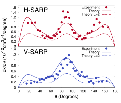
Figure 4: The velocity averaged differential state-to-state rate for HD($v=1,j=2$) $\to$ HD($v=1,j=0$) in collisions with para-H₂ and ortho-H₂ for HD prepared using H-SARP and V-SARP. The solid dots are the corresponding experiment results of Perreault et al. Perreault et al. (2018a).

IV Conclusions

We have performed numerically-exact quantum scattering calculations for low energy collisions of quantum-state prepared HD with H₂, finding excellent agreement with experiment for the angular distribution of scattered HD. Our computations provide a complete numerical simulation of the experiment with full quantum-state resolution, including, orientation of the HD molecule relative to the molecular beam axis. We were able to unravel the stereodynamics of the collision process and attribute the observed angular distribution to a single $L=2$ shape resonance in the incoming channel. This demonstrates the enormous potential of low energy beam experiments for studying inelastic collision processes at the single partial wave level, and the unique insights that can be gained in the collision dynamics when combined with numerically-exact scattering calculations. The excellent agreement between theory and experiment for this benchmark system also provides an independent confirmation of the accuracy of the H₂-H₂ interaction potential for collisional studies near 1 K, a regime also of significant interest in astrophysics.

References

- Perreault et al. (2018a) W. E. Perreault, N. Mukherjee, and R. N. Zare, Nat. Chem. 10, 561 (2018a).
- Bernstein et al. (1987) R. B. Bernstein, D. R. Herschbach, and R. D. Levine, J. Phys. Chem. 91, 5365 (1987).
- Zare (1998) R. N. Zare, Science 279, 1875 (1998).
- Aldegunde et al. (2005) J. Aldegunde, M. P. de Miranda, J. M. Haigh, B. K. Kendrick, V. Sáez-Rábanos, and F. J. Aoiz, J. Phys. Chem. A 109, 6200 (2005).
- Wynar et al. (2000) R. Wynar, R. S. Freeland, D. J. Han, C. Ryu, and D. J. Heinzen, Science 287, 1016 (2000).
- Regal et al. (2003) C. A. Regal, C. Ticknor, J. L. Bohn, and D. S. Jin, Nature 424, 47 (2003).
- Sawyer et al. (2007) B. C. Sawyer, B. L. Lev, E. R. Hudson, B. K. Stuhl, M. Lara, J. L. Bohn, and J. Ye, Phys. Rev. Lett. 98, 253002 (2007).
- Shuman et al. (2010) E. S. Shuman, J. F. Barry, and D. DeMille, Nature 467, 820 (2010).
- Hummon et al. (2013) M. T. Hummon, M. Yeo, B. K. Stuhl, A. L. Collopy, Y. Xia, and J. Ye, Phys. Rev. Lett. 110, 143001 (2013).
- Akerman et al. (2017) N. Akerman, M. Karpov, Y. Segev, N. Bibelnik, J. Narevicius, and E. Narevicius, Phys. Rev. Lett. 119, 073204 (2017).
- Anderegg et al. (2017) L. Anderegg, B. L. Augenbraun, E. Chae, B. Hemmerling, N. R. Hutzler, A. Ravi, A. Collopy, J. Ye, W. Ketterle, and J. M. Doyle, Phys. Rev. Lett. 119, 103201 (2017).
- Truppe et al. (2017) S. Truppe, H. Williams, M. Hambach, L. Caldwell, N. Fitch, E. Hinds, B. Sauer, and M. Tarbutt, Nat. Phys. 13, 1173 (2017).
- Henson et al. (2012) A. B. Henson, S. Gersten, Y. Shagam, J. Narevicius, and E. Narevicius, Science 338, 234 (2012).
- Jankunas et al. (2014) J. Jankunas, B. Bertsche, K. Jachymski, M. Hapka, and A. Osterwalder, J. Chem. Phys. 140, 244302 (2014).
- Klein et al. (2017) A. Klein, Y. Shagam, W. Skomorowski, P. S. Żuchowski, M. Pawlak, L. M. Janssen, N. Moiseyev, S. Y. Van De Meerakker, A. van der Avoird, C. P. Koch, et al., Nat. Phys. 13, 35 (2017).
- Perreault et al. (2018b) W. E. Perreault, N. Mukherjee, and R. N. Zare, Chem. Phys. (2018b).
- Ospelkaus et al. (2010) S. Ospelkaus, K.-K. Ni, D. Wang, M. H. G. de Miranda, B. Neyenhuis, G. Quéméner, P. S. Julienne, J. L. Bohn, D. S. Jin, and J. Ye, Science 327, 853 (2010).
- Knoop et al. (2010) S. Knoop, F. Ferlaino, M. Berninger, M. Mark, H.-C. Nägerl, R. Grimm, J. P. D’Incao, and B. D. Esry, Phys. Rev. Lett. 104, 053201 (2010).
- Rui et al. (2017) J. Rui, H. Yang, L. Liu, D.-C. Zhang, Y.-X. Liu, J. Nan, Y.-A. Chen, B. Zhao, and J.-W. Pan, Nat. Phys. 13, 699 (2017).
- Perreault et al. (2017) W. E. Perreault, N. Mukherjee, and R. N. Zare, Science 358, 356 (2017).
- Wolf et al. (2017) J. Wolf, M. Deiß, A. Krükow, E. Tiemann, B. P. Ruzic, Y. Wang, J. P. D’Incao, P. S. Julienne, and J. H. Denschlag, Science 358, 921 (2017).
- van der Poel et al. (2018) A. P. P. van der Poel, P. C. Zieger, S. Y. T. van de Meerakker, J. Loreau, A. van der Avoird, and H. L. Bethlem, Phys. Rev. Lett. 120, 033402 (2018).
- Amarasinghe and Suits (2017) C. Amarasinghe and A. G. Suits, J. Phys. Chem. Lett 8, 5153 (2017).
- Chandler (2010) D. W. Chandler, J. Chem. Phys. 132, 110901 (2010).
- Bergeat et al. (2015) A. Bergeat, J. Onvlee, C. Naulin, A. van der Avoird, and M. Costes, Nat. Chem. 7, 349 (2015).
- Lin and Guo (2002) S. Y. Lin and H. Guo, J. Chem. Phys. 117, 5183 (2002).
- Pogrebnya and Clary (2002) S. K. Pogrebnya and D. C. Clary, Chem. Phys. Lett. 363, 523 (2002).
- Gatti et al. (2005) F. Gatti, F. Otto, S. Sukiasyan, and H.-D. Meyer, J. Chem. Phys. 123, 174311 (2005).
- Quéméner et al. (2008) G. Quéméner, N. Balakrishnan, and R. V. Krems, Phys. Rev. A 77, 030704 (2008).
- Hinde (2008) R. J. Hinde, J. Chem. Phys. 128, 154308 (2008).
- dos Santos et al. (2011) S. F. dos Santos, N. Balakrishnan, S. Lepp, G. Quéméner, R. C. Forrey, R. J. Hinde, and P. C. Stancil, J. Chem. Phys. 134, 214303 (2011).
- Balakrishnan et al. (2011) N. Balakrishnan, G. Quéméner, R. C. Forrey, R. J. Hinde, and P. C. Stancil, J. Chem. Phys. 134, 014301 (2011).
- Boothroyd et al. (1991) A. I. Boothroyd, J. E. Dove, W. J. Keogh, P. G. Martin, and M. R. Peterson, J. Chem. Phys. 95, 4331 (1991).
- Patkowski et al. (2008) K. Patkowski, W. Cencek, P. Jankowski, K. Szalewicz, J. B. Mehl, G. Garberoglio, and A. H. Harvey, J. Chem. Phys. 129, 094304 (2008).
- (35) R. Krems, TwoBC – quantum scattering program, University of British Columbia, Vancouver, Canada, 2006.
- Quéméner and Balakrishnan (2009) G. Quéméner and N. Balakrishnan, J. Chem. Phys. 130, 114303 (2009).
- Yang et al. (2015) B. Yang, P. Zhang, X. Wang, P. Stancil, J. Bowman, N. Balakrishnan, and R. Forrey, Nat. Commun. 6, 6629 (2015).
- Yang et al. (2018) B. Yang, P. Zhang, C. Qu, X. H. Wang, P. C. Stancil, J. M. Bowman, N. Balakrishnan, B. M. McLaughlin, and R. C. Forrey, J. Phys. Chem. A 122, 1511 (2018).
- Yang et al. (2016) B. Yang, X. H. Wang, P. C. Stancil, J. M. Bowman, N. Balakrishnan, and R. C. Forrey, J. Chem. Phys. 145, 224307 (2016).
- dos Santos et al. (2013) S. F. dos Santos, N. Balakrishnan, R. C. Forrey, and P. C. Stancil, J. Chem. Phys. 138, 104302 (2013).
- Arthurs and Dalgarno (1960) A. M. Arthurs and A. Dalgarno, Proc. Roy. Soc., Ser. A 256, 540 (1960).
- Schaefer and Meyer (1979) J. Schaefer and W. Meyer, J. Chem. Phys. 70, 344 (1979).