Minimum Quadratic Helicity States

Abstract

Building on previous results on the quadratic helicity in magnetohydrodynamics (MHD) we investigate particular minimum helicity states. Those are eigenfunctions of the curl operator and are shown to constitute solutions of the quasi-stationary incompressible ideal MHD equations. We then show that these states have indeed minimum quadratic helicity.

1 Introduction

Magnetic field line topology has been recognized to be a crucial part in the evolution of magnetic fields in magnetohydrodynamics (MHD) [21, 16, 19, 10, 14, 12, 8, 23, 20, 6]. The most used quantifier of the field’s topology is the magnetic helicity [15, 4, 5, 9] which measures the linking, braiding and twisting of the field lines. Through Arnold’s inequality [4] it imposes a lower bound for the magnetic energy. As the magnetic helicity is a (second order) invariant under non-dissipative evolution (non-resistive) it imposes restrictions on the evolution of the magnetic field. Further topological invariants can be found of third and fourth order [18] which can be non-zero even for zero magnetic helicity, as well as the field line helicity [22, 17] that measures a weighted averaged helicity along magnetic field lines, and the two quadratic helicities [2].

In this work we consider the quadratic helicity of special cases of magnetic fields. Those are eigenvectors of the curl operator, which implies that the field is also force-free, i.e. the Lorentz force vanishes. We first introduce these fields and discuss some general properties by applying the Lobachevskii geometry to MHD. Then we show that they constitute quasi-stationary solutions of the ideal incompressible MHD equations by using geodesic flows [7]. This is done on special manifolds equipped with a prescribed Riemannian metric, which corresponds to a dynamics of the Anosov type. Using the geodesic flow construction, we apply the results from hyperbolic dynamics to calculate higher invariants of the magnetic field of which presented calculations of quadratic helicities are the simplest examples. Finally, we show that those fields constitute minimal quadratic helicity states.

2 Eigenfunctions of the curl operator

2.1 Positive Eigenfunction

Let $S^{3}$ be the standard $3$-sphere

(1) $$S^{3}=\{z_{1},z_{2}|z_{1}\bar{z_{1}}+z_{2}\bar{z_{2}}=1\},\quad z_{1},z_{2}\in\mathbb{C},$$

equipped with the standard Riemannian metric $g$. Let $\Theta:S^{1}\times S^{3}\to S^{3}$ be the standard action of the unit complex circle, given by

$$\Theta(\varphi;z_{1},z_{2})=(z_{1}\exp({\bf i}\varphi),z_{2}\exp({\bf i}\varphi)).$$

Let ${\bf B}_{\rm right}={\rm d}{}\Theta/{\rm d}{}\varphi$ be the Hopf magnetic field on $S^{3}$, which is tangent to the Hopf fibers (fibers of $\Theta$).

Lemma 2.1.

Consider the operator ${\bf{rot}}$ on the Riemannian manifold $(S^{3},g)$ (see for the definition [3] I.9.5), we get:

(2) $${\bf{rot}}{\bf B}_{\rm right}({\bf x})=2{\bf B}_{\rm right}({\bf x}),\quad{\bf x}\in S^{3}.$$

Proof 2.2.

This is Example 5.2 in [4] However, we show here direct calculations of this lemma. For that we define the curve $\Theta$ on $\mathbb{R}^{4}$ rather than on $\mathbb{C}^{2}$:

(3) $$\Theta(\varphi,x_{0},x_{1},x_{2},x_{3}) = \left(x_{0}\cos(\varphi)-x_{1}\sin(\varphi),x_{0}\sin(\varphi)+x_{1}\cos(\varphi),\right.$$

$$\left.x_{2}\cos(\varphi)-x_{3}\sin(\varphi),x_{2}\sin(\varphi)+x_{3}\cos(\varphi)\right),$$

with the coordinates $x_{0}$, $x_{1}$, $x_{2}$ and $x_{3}$. From that we can compute ${\bf B}_{\rm right}={\rm d}{}\Theta/{\rm d}{}\varphi$ from which we define the associated differential one-form on $\mathbb{R}^{4}$:

(4) $$\beta_{\rm right}^{\rm R4}=B^{0}_{\rm right}{\rm d}{}x^{0}+B^{1}_{\rm right}{\rm d}{}x^{1}+B^{2}_{\rm right}{\rm d}{}x^{2}+B^{3}_{\rm right}{\rm d}{}x^{3}.$$

We now define the mapping between points on the three-sphere $S^{3}$ and $\mathbb{R}^{4}$:

(5) $$\Psi = (x_{0},x_{1},x_{2},x_{3})$$

$$x_{0} = \cos(\theta_{1})$$

$$x_{1} = \sin(\theta_{1})\cos(\theta_{2})$$

$$x_{2} = \sin(\theta_{1})\sin(\theta_{2})\cos(\theta_{3})$$

$$x_{3} = \sin(\theta_{1})\sin(\theta_{2})\sin(\theta_{3}),$$

with the coordinates of $S^{3}$: $\theta_{1}\in[0,2\pi)$, $\theta_{2}\in[0,\pi]$ and $\theta_{3}\in[0,\pi]$. We can now compute the differential one-form $\beta_{\rm right}^{\rm R4}$ on $S^{3}$ as the pull-back under the mapping $\Psi$

$$\beta_{\rm right}^{\rm S3} = \Psi^{*}\beta_{\rm right}^{\rm R4}$$

$$= \cos(\varphi)\cos(\theta_{2}){\rm d}{}\theta^{1}-\cos(\varphi)\cos(\theta_{1})\sin(\theta_{1})\sin(\theta_{2}){\rm d}{}\theta^{2}$$

$$+\cos(\varphi)\sin^{2}(\theta_{1})\sin^{2}(\theta_{2}){\rm d}{}\theta^{3}$$

The curl operation on the vector field ${\bf B}_{\rm right}^{S3}$ corresponds to the exterior differential of the one-form $\beta_{\rm right}^{S3}$ which results in a two-form ${\rm d}{}\beta_{\rm right}^{S3}$. We take it’s Hodge-dual $\star{\rm d}{}\beta_{\rm right}^{S3}$, compare it with $\beta_{\rm right}^{S3}$ and find

(7) $$\star{\rm d}{}\beta_{\rm right}^{S3} = 2\cos(\varphi)\cos(\theta_{2}){\rm d}{}\theta^{1}-2\cos(\varphi)\cos(\theta_{1})\sin(\theta_{1})\sin(\theta_{2}){\rm d}{}\theta^{2}$$

$$+2\cos(\varphi)\sin^{2}(\theta_{1})\sin^{2}(\theta_{2}){\rm d}{}\theta^{3}.$$

Hence the result

(8) $$\star{\rm d}{}\beta_{\rm right}^{\rm S3}=2\beta_{\rm right}^{\rm S3},$$

which corresponds to equation (2).

The left transformation of $S^{3}$ (see the beginning of the next section for the right transformation) is transitive and is an isometry This isometry commutes with the curl operator and keeps the Hopf fibration (which is determined by the right ${\bf i}$-multiplication). This proves the equation (2) at an arbitrary point on $S^{3}$.

Remark 2.3.

Equation (2) corresponds with Lemma 2.6 for $\Lambda(S^{2})$. The natural metric on a Hopf fiber for $\Lambda(S^{2})\to S^{2}$ is proportional to the natural metric of the Hopf fiber for $S^{3}\to S^{2}$ with the coefficient $2$, because $S^{3}\to\Lambda(S^{2})$ is the double covering.

2.2 Negative Eigenfunction

The magnetic field ${\bf B}_{\rm right}$ is generalized by the following construction. Take $S^{3}$ as the unit quaternions $\left\{a+b{\bf i}+c{\bf j}+d{\bf k}\middle|a^{2}+b^{2}+c^{2}+d^{2}=1\right\}$. Take a tangent quaternion $\xi\in T_{{\bf x}=1}(S^{3})$ and define the vector-field ${\bf B}_{\rm right}({\bf x})={\bf x}\xi$ by the right multiplication. In the case $\xi={\bf i}$ we get the vector-field from Lemma 2.1. In the case $\xi={\bf j}$ the vector-field ${\bf B}_{\rm right}$ is not invariant with respect to the action $\Theta$ along the Hopf fibers. To get the invariant vector-field ${\bf B}_{\rm left}$ we define ${\bf B}_{\rm left}={\bf j}{\bf x}$, ${\bf x}\in S^{3}$, by the left multiplication. We get:

(9) $${\bf{rot}}{\bf B}_{\rm left}({\bf x})=-2{\bf B}_{\rm left}({\bf x}),\quad{\bf x}\in S^{3}.$$

This follows from the fact that the conjugation

$$\left(a+b{\bf i}+c{\bf j}+d{\bf k}\right)^{*}\mapsto a-b{\bf i}-c{\bf j}-d{\bf k},$$

which is an antiautomorphism and an isometry, transforms right vector-fields to left-vector fields. This antiautomorphism changes the orientation on $S^{3}$. Therefore, equation (2) for the vector-field ${\bf B}_{\rm right}$ implies equation (9) for ${\bf B}_{\rm left}$.

The vector-field ${\bf B}_{\rm left}$ admits an alternative description by means of geodesic flows on the Riemann sphere $S^{2}$ in the following way. The sphere $(S^{3},g)$ is diffeomorphic to the universal (2-sheeted) covering over the manifold $SO(3)$, equipped with the standard Riemannian metric. The manifold $SO(3)$ is diffeomorphic to the spherization of the tangent bundle over the standard 2-sphere $S^{2}$, denoted by $\Lambda(S^{2})$. The projection $p_{1}({\bf x}):\Lambda(S^{2})\to S^{2}$, ${\bf x}\in\Lambda(S^{2})$ is well-defined. A circle fiber over $p_{1}({\bf x})\in S^{2},{\bf x}\in\Lambda(S^{2})$ is visualized as a great circle $S^{1}\subset S^{2}$, with the center $p_{1}({\bf x})$, equipped with the prescribed orientation.

Consider the spherization of the (trivial) tangent bundle over the plane $\Lambda(\mathbb{R}^{2})$. Denote by ${\bf B}_{\rm left}$ the magnetic field on $\Lambda(\mathbb{R}^{2})$, which is tangent to the geodesic flow. The natural Riemannian metric $h$ on $\Lambda(\mathbb{R}^{2})$ coincides with the standard metric of the decomposition $\Lambda(\mathbb{R}^{2})=\mathbb{R}^{2}\times S^{1}$.

Lemma 2.4.

The equation:

(10) $${\bf{rot}}{\bf B}_{\rm left}({\bf x})=-{\bf B}_{\rm left}({\bf x}),\quad{\bf x}\in\Lambda(\mathbb{R}^{2}),$$

in the metric $h$ is satisfied.

Proof 2.5.

The manifold $\Lambda(\mathbb{R}^{2})$ is equipped with the projection $p_{2}({\bf x}):\Lambda(\mathbb{R}^{2})\to\mathbb{R}^{2}$. Take the Cartesian coordinates in $\mathbb{R}^{2}$ and the coordinate $\varphi$ along fibers. In the coordinates $(x,y,\varphi)$ on $\Lambda(\mathbb{R}^{2})$ the magnetic field ${\bf B}_{0}$ is defined as $B_{x}=\cos(\varphi),B_{y}=\sin(\varphi),B_{\varphi}=0$. The components of ${\bf{rot}}{\bf B}_{0}$ are defined by the determinant:

(14) $$\begin{array}[]{ccc}\frac{\partial}{\partial x}&\frac{\partial}{\partial y}&\frac{\partial}{\partial\varphi}\\ B_{x}&B_{y}&B_{\varphi}\\ \ast&\ast&\ast\\ \end{array}.$$

Lemma 2.4 is proven by following calculations: at ${\bf x}$ for ${\bf B}={\bf B}_{\rm right}$: $B_{x}=0,B_{y}=1,B_{x}=0$; $({\bf{rot}}{\bf B})_{y}=\frac{\partial B_{\varphi}}{\partial x}-\frac{\partial B_{x}}{\partial\varphi}=1$, $({\bf{rot}}{\bf B})_{x}=({\bf{rot}}{\bf B})_{z}=0$.

2.3 Eigenfunctions on Different Manifolds

Consider the spherization of the tangent bundle over the Riemannian sphere $\Lambda(S^{2})$ and the spherization of the tangent bundle over the Lobachevskii plane $\Lambda(L^{2})$. The spaces $\Lambda(S^{2})$ and $\Lambda(L^{2})$ are equipped with the standard Riemannian metrics $g_{S}$ and $g_{L}$. The metrics correspond to the standard metrics on $S^{2}$ and $L^{2}$ and the standard metric on the circle. Denote by ${\bf B}_{\rm left}$ the magnetic field on $(S^{3},g)$ as the pull-back of the magnetic field on $\Lambda(S^{2})$, which is tangent to the geodesic flow. The geodesic magnetic fields on $\Lambda(S^{2})$, $\Lambda(L^{2})$ are also denoted by ${\bf B}_{\rm left}$.

Lemma 2.6.

The equation (10) is satisfied on $(\Lambda(S^{2}),g_{S})$ and $(\Lambda(L^{2}),g_{L})$.

Proof 2.7.

Let us prove the lemma for the space $(\Lambda(S^{2}),g_{S})$. For the points $\hat{{\bf x}}\in\Lambda(S^{2})$ and $\hat{{\bf y}}\in\Lambda(\mathbb{R}^{2})$ in the corresponding neighborhoods $\hat{{\bf x}}\in\hat{V}_{\hat{\bf x}}\subset\Lambda(S^{2})$, $\hat{{\bf y}}\in U_{\hat{{\bf y}}}\subset\Lambda(\mathbb{R}^{2})$, let us construct a mapping ${\rm pr}:\hat{V}_{\hat{{\bf x}}}\to\hat{U}_{\hat{{\bf y}}}$, which is an isometry in vertical lines and is a local isometry in horizontal planes up to $O(r^{2})$, where $r$ is the distance in $U_{\hat{\bf x}}$.

Consider the natural Riemannian metric $g_{S}$ on $\Lambda(S^{2})$ in $\hat{V}_{\hat{{\bf x}}}$ locally near a point $\hat{{\bf x}}\in\Lambda(S^{2})$. In horizontal planes the metric $g_{S}$ agrees with the Riemannian metric $h$ on the standard sphere $S^{2}\subset\mathbb{R}^{3}$. In vertical planes the metric $g_{S}$ corresponds to angles trough points on $S^{2}$.

Take a tangent plane $T_{{\bf x}}\subset\mathbb{R}^{3}$ at the point ${\bf x}=p_{1}(\hat{\bf x})\in S^{2}$, where $p_{1}:\Lambda(S^{2})\to S^{2}$ is the natural projection along vertical coordinates. Consider the stereographic projection $P$ from $S^{2}_{{\bf x}}$ into $T_{{\bf x}}$, which keeps the points: $P({\bf x})=({\bf y})$, ${\bf y}=p_{2}(\hat{\bf y})$, $p_{2}:\Lambda(\mathbb{R}^{2})\to\mathbb{R}^{2}$. The projection $P$ is a conformal map and is an isometry up to $O(r^{2})$ near ${\bf x}$. This stereographic projection induces the required mapping ${\rm pr}:\hat{V}_{{\bf x}}\to\hat{U}_{{\bf y}}$.

From equation (10) for ${\bf B}_{{\rm left};\mathbb{R}^{2}}$ on $\Lambda(\mathbb{R}^{2})$ at ${\bf y}$ we get the the same equation for $P^{\ast}({\bf B}_{{\rm left};\mathbb{R}^{2}})$ on $\Lambda(S^{2})$ at ${\bf x}$ in the induced metric $P^{\ast}(g_{S})$. After we change the metric $P^{\ast}(g_{S})$ on $\Lambda(S^{2})$ into the natural metric $g_{S}$, we get the same equation for $P^{\ast}({\bf B}_{{\rm left};\mathbb{R}^{2}})$ at ${\bf x}$, because the curl operator is a first-order operator.

The last required fact is the following: $P^{\ast}({\bf B}_{{\rm left};S^{2}})$ in the standard metric $g_{S}$ coincides with the geodesic vector-field ${\bf B}_{\rm left}$ on $\Lambda(\mathbb{R}^{2})$.

To prove the lemma for $(\Lambda(L^{2}),g_{L})$ we use analogous arguments: instead of the stereographic projection $S^{2}\to\mathbb{R}^{2}$, we take a conformal mapping by the identity $L^{2}\subset\mathbb{R}^{2}$, where the Lobachevskii plane $L^{2}$ is considered as the Poincarè unit disk on the Euclidean plane. At the central point of the disk the mapping $L^{2}\subset\mathbb{R}^{2}$ is an isometry.

We now generalize the example of Lemma 2.6 for magnetic fields in domains with non-homogeneous density (volume-forms). Let $(A,{\bf x})$ be a complex neighborhood of a point ${\bf x}$, equipped with a Riemannian metric $g_{A}$ of a constant negative scalar curvature surface. In the example we get $A\subset L^{2}$, where $L^{2}$ is the Lobachevskii plane. Let $(D,{\bf y})$ be a complex neighborhood of a point in the Riemannian sphere $S^{2}$, equipped with the standard Riemannian metric $g_{D}$ of a constant positive scalar curvature.

Let $f:(A,{\bf x})\to(D,{\bf y})$ be a conformal germ of open surfaces $A$ and $D$ with metrics $g_{A}$, $g_{D}$. Consider the natural extension $F:(U,\hat{{\bf x}})\to(V,\hat{{\bf y}})$ of the germ $f$, where $\hat{{\bf x}}\in U\subset\Lambda(A)$, $\hat{{\bf y}}\in V\subset\Lambda(D)$ are neighborhoods of points $\hat{{\bf x}},p_{A}(\hat{{\bf x}})={\bf x},p_{A}:\Lambda(A)\to A$, $\hat{{\bf y}},p_{D}(\hat{{\bf y}})={\bf y},p_{D}:\Lambda(D)\to D$; $U$, $V$ are equipped with the standard Riemannian metrics $g_{U}$ and $g_{V}$ correspondingly, which are defined using the metrics $g_{A}$ and $g_{D}$.

Let us consider an extra copy of $U\subset\Lambda(L^{2})$ with an exotic metric, which will be denoted by $(\tilde{U},h_{\tilde{U}})$. Define in $\tilde{U}\subset\Lambda(L^{2})$ the Riemannian metric $h_{\tilde{U}}$, which coincides with $g_{U}$ along horizontal planes $A\subset(U,\hat{{\bf x}})$ of $p_{U}:(U,\hat{{\bf x}})\to(\Lambda(A),{\bf x})$ and coincides with ${\bf k}^{-1}({\bf x})g_{U}$ along the vertical fiber of $p_{U}$, where ${\bf k}({\bf x})$ is a real positive-valued function, defined by the Jacobian ${\bf k}^{2}({\bf x})$ of ${\rm d}{}f$ at ${\bf x}$ of the differential ${\rm d}{}f:(T(A),{\bf x})\to(T(D),{\bf y})$.

Let us consider an extra copy of $V\subset\Lambda(S^{2})$ with an exotic metric, which is denoted by $(\tilde{V},h_{\tilde{V}})$. Define in $\tilde{V}\subset\Lambda(S^{2})$ the Riemannian metric $h_{\tilde{V}}$ that coincides with ${\bf k}^{-1}({\bf x}=f^{-1}({\bf y}))g_{V}$.

Let $\bar{V}\to V$, $\bar{V}\subset S^{3}$, be the natural double covering, which is the isometry on horizontal planes and is the multiplication by $2$ in each vertical circle fibers of the standard projection $p:S^{3}\to\Lambda(S^{2})$. Define in $\bar{V}$ a Riemannian metric $g_{\bar{V}}$ that coincides with $g_{V}$ along horizontal planes and with $\frac{1}{2}g_{V}$ along vertical fibers.

The Riemannian metrics $g_{U}$, $h_{\tilde{U}}$, $h_{\tilde{V}}$, $g_{V}$ and $g_{\bar{V}}$ determine the volume 3-forms ${\rm d}{}U$ (the standard form in $\Lambda(L^{2})$), ${\rm d}{}\tilde{U}$, ${\rm d}{}\tilde{V}$, ${\rm d}{}V$ (the standard form in $\Lambda(S^{2})$) and ${\rm d}{}\bar{V}$ (the standard form in $S^{3}$) in $U$, $\tilde{U}$, $\tilde{V}$, $V$ and $\bar{V}$ correspondingly. Recall $A\subset L^{2}$ with the standard 2-volume form ${\rm d}{}L$ on the Lobachevskii plane. The volume form ${\rm d}{}\tilde{U}$ is defined by ${\rm d}{}\tilde{U}={\bf k}({\bf x}){\rm d}{}U$, where ${\rm d}{}U$ is the standard volume form in $U$, which is the product of the horizontal standard 2-form ${\rm d}{}L$ on the Lobachevskii plane with the the standard vertical 1-form on the circle. Analogously, ${\rm d}{}\tilde{V}={\bf k}^{-2}({\bf y}){\rm d}{}V$, where ${\rm d}{}V$ is the standard volume form on $V=\tilde{V}\subset\Lambda(S^{2})$. The volume forms ${\rm d}{}V$, ${\rm d}{}\bar{V}$ coincide with the standard volume forms (${\rm d}{}V$ is the restriction of the standard volume form on $\Lambda(S^{2})$, ${\rm d}{}\bar{V}$ is the restriction of the standard volume form on $S^{3}$; ${\rm d}{}\bar{V}=2p^{\ast}{\rm d}{}V$, where $\bar{V}$ is standardly identified with $V$ by $p:\bar{V}\to V$). The volume forms ${\rm d}{}V$, ${\rm d}{}\bar{V}$ are equipped with the density functions $\rho_{V}(\hat{\bf y})={\bf k}^{-2}({\bf y}=p_{V}(\hat{\bf y}))$, $\rho_{\bar{V}}(\bar{\bf y})={\bf k}^{-2}({\bf y}=p_{V}\circ p(\bar{\bf y}))$.

Let ${\bf B}_{U}$ be the magnetic field (horizontal) in $U$ with the metric $g_{U}$, which is defined by the geodesic flows in $A$ with the metric $g_{A}$. Define the magnetic field ${\bf B}_{{\rm left};\tilde{U}}$ in $\tilde{U}$ with the metric $h_{\tilde{U}}$ by ${\bf B}_{{\rm left};\tilde{U}}={\bf B}_{U}$.

By construction, the metrics $h_{\tilde{U}}$ and $h_{\tilde{V}}$ agree (are isometric): $F_{\ast}(h_{\tilde{U}})=h_{\tilde{V}}$. Denote by ${\bf B}_{{\rm left};\tilde{V}}$ the magnetic field $F_{\ast}({\bf B}_{{\rm leftU};\tilde{U}})$ in $\tilde{V}\subset\Lambda(S^{2})$ with the metric $h_{\tilde{V}}$. Denote by ${\bf B}_{{\rm left};V}$ the magnetic field ${\bf k}^{-3}(\hat{\bf y}){\bf B}_{{\rm left};\tilde{V}}$ in $V\subset\Lambda(S^{2})$ with the standard metric $g_{V}$ and with the variable density $\rho_{V}(\hat{\bf y})$. Denote by ${\bf B}^{S3}_{{\rm left}\bar{V}}$ the magnetic field ${\bf k}^{-3}(p(\bar{\bf y}))p^{\ast}({\bf B}_{{\rm left};\vec{\bf V}})$ in $\bar{V}\subset S^{3}$ with the standard spherical metric $g_{\bar{V}}$ and with the variable density $\rho_{\bar{V}}(\bar{\bf y})$.

Lemma 2.8.

1. In the domain $\tilde{U}$ the following equation is satisfied:

   (17) $$\begin{array}[]{cc}{\bf{div}}({\bf B}_{{\rm left};\tilde{U}})=0;\qquad{\bf{rot}}{\bf B}_{{\rm left};\tilde{U}}(\hat{{\bf x}})=-{\bf k}({\bf x}){\bf B}_{{\rm left};\tilde{U}}(\hat{{\bf x}}),\\ \hat{{\bf x}}\in\tilde{U},\quad{\bf x}=p_{\tilde{U}}(\hat{{\bf x}})\in A,\end{array}$$

   where ${\bf{rot}}$ and ${\bf{div}}$ are defined for the Riemannian metric $h_{\tilde{U}}$ with the density $\rho_{U}(\hat{\bf x})$.

2. In the domain $V\subset\Lambda(S^{2})$ the following equation is satisfied:

   (20) $$\begin{array}[]{cc}{\bf{div}}({\bf B}_{{\rm left};V}(\hat{\bf y}))=0;\qquad{\bf{rot}}{\bf B}_{{\rm left};V}(\hat{\bf y})=-{\bf B}_{{\rm left};V}(\hat{{\bf y}}),\\ \hat{{\bf y}}\in V,\quad{\bf y}=p_{V}(\hat{{\bf y}})\in D,\end{array}$$

   where ${\bf{rot}}$ is defined for the standard Riemannian metric $g_{V}$ with the density $\rho_{V}(\hat{\bf y})$.

3. In the domain $\bar{V}\subset S^{3}$ the following equation is satisfied:

   (23) $$\begin{array}[]{cc}{\bf{div}}({\bf B}_{{\rm left};\bar{V}}(\bar{\bf y}))=0;\qquad{\bf{rot}}{\bf B}_{{\rm left};\bar{V}}(\hat{\bf y})=-2{\bf B}_{{\rm left};\bar{V}}(\hat{{\bf y}}),\\ \bar{{\bf y}}\in\bar{V},\quad{\bf y}=p_{V}\circ p(\bar{{\bf y}})\in D,\end{array}$$

   where ${\bf{rot}}$ is defined for the standard spherical Riemannian metric $g_{\bar{V}}$ with the density $\rho_{\bar{V}}(\bar{\bf y})$.

Proof 2.9.

By construction, the magnetic field ${\bf B}_{U}$ satisfies equation (2.4) in $U$. The transformation from $U$ to $\tilde{U}$ is the identity, but not isometry. The first equation (17) is satisfied, because the volume form in $U$ corresponds with the metric $h_{\tilde{U}}$. The transformation ${\bf B}_{U}\mapsto{\bf B}_{{\rm left};\tilde{U}}$ is frozen-in and keeps the magnetic flow. The second equation (17) is satisfied, because the metric $h_{\tilde{U}}$ is constant in vertical fibers and the factor ${\bf k}({\bf x})$ in the right side of the equation corresponds to the partial derivatives along the vertical coordinates. This proves equation (17).

The transformation ${\bf B}_{{\rm left};\tilde{U}}\mapsto{\bf B}_{{\rm left};V}$ is decomposed into transformations

$${\bf B}_{{\rm left};\tilde{U}}\mapsto{\bf B}_{{\rm left};\tilde{V}}\mapsto{\bf B}_{{\rm left};V}.$$

The transformation ${\bf B}_{{\rm left};\tilde{U}}\mapsto{\bf B}_{{\rm left};\tilde{V}}$ is an isometry and ${\bf B}_{{\rm left};\tilde{V}}$ satisfies equation (17) in $\tilde{V}$. The transformation ${\bf B}_{{\rm left};\tilde{V}}\mapsto{\bf B}_{{\rm left};V}$ is conform with the scalar factor ${\bf k}({\bf y})$. This transformation changes equation (17) in $\tilde{V}$ into (20) in $V$ with non-uniform density.

The calculations for this transformation are as follows. Take a domain $\tilde{V}$ with local coordinates $\hat{{\bf x}}=(x,y,z)$. Take a transformation $g\mapsto\lambda g$ of the metric in $\tilde{V}$ into a metric in $V$ with a scale $\lambda(\hat{{\bf x}})>0$. The following transformation of coordinates $x\mapsto\lambda x_{1}$, $y\mapsto\lambda y_{1}$, $z\mapsto\lambda z_{1}$ is an isometric transformation of $(\tilde{V},g)$ into $(V,\lambda g)$, where $\hat{{\bf x}}_{1}=(x_{1},y_{1},z_{1})$ are the coordinates in $V$. Before the transformation we get a differential $1$-form $\beta{\rm d}{}z$ which is by assumption, a proper form of the operator $\ast\circ d$ with a proper function $-\lambda({\bf x})$ (see equations (8) with analogous calculations) in $\tilde{V}$. This implies ${\rm d}{}(\beta{\rm d}{}z)=\frac{\partial\beta}{\partial x}{\rm d}{}x\wedge{\rm d}{}z+\frac{\partial\beta}{\partial y}{\rm d}{}y\wedge{\rm d}{}z$; $\frac{\partial\beta}{\partial x}=-\lambda(\hat{\bf x})$, $\frac{\partial\beta}{\partial y}=-\lambda(\hat{\bf x})$. After the transformation we get the $1$-form $\lambda\beta{\rm d}{}z_{1}$. We have:

$${\rm d}{}(\lambda\beta{\rm d}{}z_{1})=\frac{\partial\beta}{\partial x}\lambda{\rm d}{}x\wedge{\rm d}{}z_{1}+\frac{\partial\beta}{\partial y}\lambda{\rm d}{}y\wedge{\rm d}{}z_{1}+\frac{\beta}{\lambda}\frac{\partial\lambda}{\partial x}{\rm d}{}x_{1}\wedge{\rm d}{}z_{1}+\frac{\beta}{\lambda}\frac{\partial\lambda}{\partial y}{\rm d}{}y_{1}\wedge{\rm d}{}z_{1}+$$

$$\lambda\beta{\rm d}{}x\wedge\frac{\partial}{\partial x}\left(\frac{1}{\lambda}{\rm d}{}z\right)+\lambda\beta{\rm d}{}y\wedge\frac{\partial}{\partial x}\left(\frac{1}{\lambda}{\rm d}{}z\right).$$

Using $\frac{\partial}{\partial z_{1}}=\lambda\frac{\partial}{\partial z}$, ${\rm d}{}x\wedge\frac{\partial}{\partial x}(\frac{1}{\lambda}{\rm d}{}z)=-\frac{1}{\lambda^{2}}\frac{\partial\lambda}{\partial x}{\rm d}{}x\wedge{\rm d}{}z$, ${\rm d}{}y\wedge\frac{\partial}{\partial y}(\frac{1}{\lambda}{\rm d}{}z)=-\frac{1}{\lambda^{2}}\frac{\partial\lambda}{\partial y}{\rm d}{}y\wedge{\rm d}{}z$, we have:

$${\rm d}{}(\lambda\beta{\rm d}{}z_{1})=\frac{\partial\beta}{\partial x}\lambda{\rm d}{}x\wedge{\rm d}{}z_{1}+\frac{\partial\beta}{\partial y}\lambda{\rm d}{}y\wedge{\rm d}{}z_{1}=\frac{\partial\beta}{\partial x}{\rm d}{}x_{1}\wedge{\rm d}{}z_{1}+\frac{\partial\beta}{\partial y}{\rm d}{}y_{1}\wedge{\rm d}{}z_{1}=$$

$$-\lambda({\rm d}{}x_{1}\wedge{\rm d}{}z_{1}+{\rm d}{}y_{1}\wedge{\rm d}{}z_{1}).$$

This proves that $\lambda\beta{\rm d}{}z_{1}$ is the proper $1$-form of the operator $\ast\circ{\rm d}{}$ in $V$ with the proper function $-\lambda^{-1}\lambda=-1$. Setting ${\bf k}({\bf x})=\lambda({\bf x})$, we get the required formula (20).

The transformation ${\bf B}_{{\rm left};V}\mapsto{\bf B}_{{\rm left};\bar{V}}$ is analogous to the transformation ${\bf B}_{U}\mapsto{\bf B}_{{\rm left};\tilde{U}}$. In this transformation ${\bf B}_{\rm left}$ is frozen-in and the scalar factor $2$ in the right side of the second equation (23) corresponds to the transformation of the metrics $g_{V}\mapsto g_{\bar{V}}$, which changes partial derivatives along the vertical coordinate.

3 Magnetic force-free configurations on non-homogeneous $S^{3}$

Let $P\subset L^{2}$ be the right $k$-triangle (all $k$-vertices on the absolute) on the Lobachevskii plane. Let $f_{k}:P\to S^{2}_{+}$ be the conformal transformation (the Picard analytic function in the case $k=3$) of the square ($k$-angle) onto the upper hemisphere of the Riemannian sphere $S^{2}$. The vertices $v_{1},v_{2},\dots,v_{k}$ of $P$ are mapped into points $f(v_{1}),f(v_{2}),\dots,f(v_{k})$ at the equator $S^{1}\subset S^{2}$ and we assume that ${\rm dist}(f(v_{1}),f(v_{2}))=\dots={\rm dist}(f(v_{k}),f(v_{1}))=\frac{2\pi}{k}$. Denote by $f:L^{2}\to S^{2}$ the branched cover with ramifications at $f(v_{1}),f(v_{2}),\dots,f(v_{k})$, which is defined as the conformal periodic extension of $f_{k}$ on the Lobachevskii plane. It is well known that $\Lambda(S^{2})=S^{3}/-1$, where on the right side of the formula is the quotient of the standard $3$-sphere by the antipodal involution. The fiber of $S^{3}\to\Lambda(S^{2})\to S^{2}$ over the points $f(v_{1}),\dots f(v_{k})$ in the base is the Hopf $k$-component link, which is denoted by $l\subset S^{3}$. For $k=3$ link $l$ consists of 3 big circles, each two circles are linked with the coefficient $+1$, Denote the Jacobian of $f$ by ${\bf k}^{2}({\bf x})$, ${\bf x}\in P$, ${\bf y}=f({\bf x})\in S^{2}$. Statement (i) of the following lemma is a corollary from Theorem 2.8.

Theorem 3.1.

Assume $k\geq 3$ is fixed.

1. For magnetic force-free field ${\bf B}_{\rm left}$ on $S^{3}\setminus l$ with the standard Riemannian metric $g$ and the density function $\rho(\hat{\bf y})={\bf k}^{-2}({\bf y})$, ${\bf y}=p(\hat{\bf y})$, with the standard Hopf bundel $p:S^{3}\to S^{2}\to\Lambda(S^{2})$, there are $k$-component exceptional fibers $l\subset S^{3}$ with an infinite density.

2. The $k$-component pinch curve $l$ of the magnetic field ${\bf B}_{\rm left}$ is the standard $k$-component Hopf link in $S^{3}$. The components of $l$ are preimages of points $f(v_{1}),f(v_{2}),\dots,f(v_{k})$ by the projection $p:S^{3}\to\Lambda(S^{2})$.

3. In the case $k=3$ the scalar factor of the density function $\sqrt{\rho(\hat{\bf y})}={\bf k}^{-1}({\bf y})$ in equation (17) has an asymptotic $(-z\ln(z))^{-1}$ near $l$, where $z$ is the distance from $\hat{\bf y}$ to $l$. The magnetic field has the asymptotic $(-z\ln(z))^{-1}$ for $z\to 0+$. The magnetic energy $\int B^{2}\ {\rm d}{}\Omega$, where $B^{2}(\hat{\bf y})={\bf k}^{-2}(\hat{\bf y})$ and $\hat{{\bf y}}\in\Omega=S^{3}\setminus l$, has the asymptotic $\simeq\int^{+\varepsilon}_{0}(z\ln^{2}(z))^{-1}\ {\rm d}{}z<+\infty$ near a component of a cusp curve $l$, in the standard metric on $S^{3}$.

4. In the case $k=3$, ${\bf B}_{{\rm left};3}$ is projected to tangents along trajectories of the Lorenz attractor [11, 7] by a 12-sheeted branching covering $S^{3}\setminus l\to S^{3}\setminus l^{\prime}$, which transforms $l$ into the exceptional trefoil $l^{\prime}$ of the Lorenz attractor.

5. The stereographic projection $S^{3}\setminus{pt}\to\mathbb{R}^{3}$ transforms ${\bf B}_{\rm left}$ into a force-free magnetic field with a finite magnetic energy in non-homogeneous isotropic space $\mathbb{R}^{3}$. This construction is analogous to [13].

Proof 3.2.

$\rm{(iii)}$

Let $H^{\uparrow}$ be the upper half-plane with the complex coordinate, denoted by $w$, $H^{\uparrow}\equiv L$, where $L$ is the Lobachevskii plane, equipped with the standard conformal metric, $H^{\downarrow}$ be the lower half-plane, $H_{+}$ be the right half-plane $H_{+}=\{w\in L,|\Re w>0\}$ and $H_{-}$ be the left half-plane. We identify $H^{\downarrow}$ with the Lobachevskii plane $L$, $H_{-}$ with the Riemannian half-sphere. Let $D=\{w\in H^{\uparrow},|\tau|>1,|\Re w|<1\}$ be the triangle in $H^{\uparrow}$. Let us consider the analytic function $F:D\to H_{+}$, $F(\infty)=\infty$, $F(+1)={\bf i}$, $F(-1)=-{\bf i}$. From the conditions we get $F({\bf i})=0$.

Take the triangle $C=\{a=v_{1},c=v_{2},-c=v_{3}\}$ on $H^{\downarrow}$, $a=0,c=+1$. The considered triangle is mapped onto the triangle $D=\{\infty,c,-c\}$ in the upper half-plane $H^{\uparrow}$ by $I_{1}:x\mapsto x^{-1}=w$ (see Figure 1).

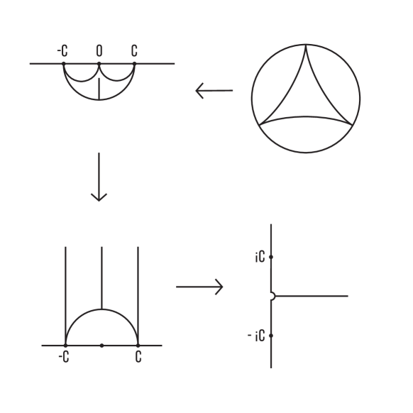
Figure 1: A transformation of the standard hyperbolic triangle onto the Riemannian half-sphere by the modular function.

The function $f:C\to H_{-}$ is the composition of the maps $I_{1}:x\mapsto x^{-1}=w$, $F:D\to H^{+}$, $F:w\mapsto F(w)=v$, $I_{2}:H_{+}\to H_{-}$, $I_{2}:v\mapsto v^{-1}=y$; $f=I_{2}\circ F\circ I_{1}:x\mapsto y$. The function $F$ is called the modular function, this function has the asymptotic $F\simeq w\mapsto\exp(\frac{i\pi w}{24})=v$, when $w\to+{\bf i}\infty$. The goal is to calculate the scalar factor ${\bf k}$ near the origin $f(0)=0$ in the target domain.

In $C\subset H^{\downarrow}$ we get the metric on the hyperbolic plane, near the origin on the boundary. The distance between two points on a vertical ray is given by the logarithmic scale. In $H_{-}$ near the origin the metric is the Euclidean metric.

We get: ${\rm d}{}y=\exp(-1/x)/x^{2}{\rm d}{}x$ and $\frac{{\rm d}{}x}{x}={\rm d}{}l$, where $l$ the distance in the domain space, $x$ is the Euclidean coordinate in the domain space, $y$ is the coordinate in the target space, which corresponds to the metric. Therefore, the scalar factor ${\bf k}^{-1}(\hat{\bf y})$ depends of the distance $z$ from the cusp $L$ in the target space $S^{3}$ with the standard metric as follows:

$${\bf k}(z)\approx-z\ln(z).$$

By this asymptotic we get the asymptotic of the magnetic energy is given by the prescribed integral over $z$.

Proof 3.3.

$\rm{(ii)}$, $\rm{(iv)}$

The Lorenz attractor by [11] coincides with the geodesic flows on the orbifold $(2,3,\infty)$ from [7]. The spherization of the tangent bundle over the orbifold $(2,3,\infty)$, which is the space of the geodesic flow, is an open manifold diffeomorphic to the complement of the trefoil in the $3$-sphere $S^{3}\setminus l^{\prime}$. The orbifold $(2,3,\infty)$ is the quotient of the Lobachevskii plane by the corresponding Fuchsian group. The fundamental domain $P^{\prime}$ of this orbifold is the triangle $\triangle OC_{1}C_{2}$ with angles $\left(\frac{\pi}{3},0,0\right)$. This triangle is contained as a $\frac{1}{3}$-triangle in the triangle $P=\triangle C_{1}C_{2}C_{3}$ with the angles $(0,0,0)$ with the vertex on the absolute (see Figure 2). The fundamental domain $Q$ of the magnetic force-free field ${\bf B}_{\rm left}$ for $k=3$ is the 2 sheet covering over the space of $S^{1}$-fibration over the union $P\cup P_{1}$ of 2 triangles $P=\triangle C_{1}C_{2}C_{3}$, $P_{1}=\triangle C_{2}C_{3}C_{4}$, which are identified along the fibration over the common edge $(C_{2}C_{3})$. Therefore, the fundamental domain $Q$ is a $6$-sheeted covering space over $\Lambda(P^{\prime})$.

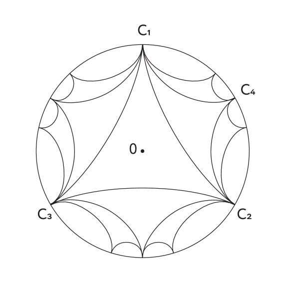
Figure 2: The covering over the orbifold $(2,3,\infty)$ for Lorenz attractor. The point $C_{4}$ is the image of $C_{3}$ with respect to the central symmetry over the fold point on $(C_{1},C_{2})$.

According to [11], the spherization of the tangent bundle $\Lambda(P^{\prime})$ over the fundamental domain $P^{\prime}$ is diffeomorphic to $S^{3}\setminus l^{\prime}$, where $l^{\prime}$ is the exceptional fiber (the trefoil), which corresponds to the vertex of the domain $P^{\prime}$, the vertex are identified by an action of the Fuchsian group. By the construction the spherization of the tangent bundle $\Lambda(P\cup P_{1})$ over the fundamental domain $P\cup P_{1}$ is diffeomorphic to $\Lambda(S^{2})\setminus l^{\prime\prime}$, $S^{3}/-1=\Lambda(S^{2})$, where $l^{\prime\prime}$ is the union of 3 exceptional fibers, which are correspondent to the vertex $f(v_{1}),f(v_{2}),f(v_{3})$ of the $\frac{1}{2}$-fundamental domain $P$. This proves that $\Lambda(S^{2})\setminus l^{\prime\prime}$ is a $6$-covering space over $S^{3}\setminus l^{\prime}$, which is branched over the trefoil $l^{\prime}$.

A neighbourhood of the exceptional trefoil $l^{\prime}$ in the Lorenz attractor is covered by a non-connected neighbourhood of $l^{\prime\prime}\subset S^{3}/-1$, which is the standard 3-Hopf link. An extra $2$-covering $S^{3}\to\Lambda(S^{2})$ determines the required $12$ covering $S^{3}\setminus l\to S^{3}\setminus l^{\prime}$, which is also branched over the trefoil $l^{\prime}$.

Remark 3.4.

By Theorem 3.1, $iii$ the magnetic field ${\bf B}_{\rm left}$ on $S^{3}\setminus l$ is compactified into the magnetic field on $S^{3}$, which tends to infinity on $l\subset S^{3}$. The magnetic field ${\bf B}_{\rm left}$ is an $Z_{6}$-equivariant with respect to the standard action $Z_{6}\times S^{3}\setminus l\to S^{3}\setminus l^{\prime}$ of the cyclic group of the order $6$, therefore the magnetic field $\hat{\bf B}_{\rm left}$ on the lens quotient $\hat{Q}=(S^{3}\setminus l)/Z_{6}$ is well-defined. The domain $\hat{Q}$ with magnetic field is a covering space over the domain with the Lorenz attractor in $S^{3}$, over the exceptional fiber $l^{\prime}\subset S^{3}$ the covering is ramified.

4 MHD-solitons

By MHD-solitons we mean quasi-stationary solutions of the ideal MHD equations. We consider MHD-solitons for the sphere $S^{3}$ with the standard metric $g$ with the constant and variable density $\rho(\hat{{\bf y}})$, $\hat{{\bf y}}\in S^{3}$, see [3] Remark 1.6 p. 262 and Remark 1.1 p. 120, for the MHD-equations on a Riemannian manifold. The density positive function $\rho(\hat{{\bf y}})$ is equivalent that the standard metric $g$ is changed $g\mapsto\rho(\hat{{\bf y}})^{-\frac{1}{3}}g$ by a conformal transformation.

A quasi-stationary solution means that the velocity field ${\bf v}$ does not depend on time (see equation (25)).

(24) $$\frac{\partial{\bf B}}{\partial t}=-\{{\bf v},{\bf B}\},$$

(25) $$\frac{\partial{\bf v}}{\partial t}=-({\bf v},\nabla){\bf v}+{\bf{rot}}{\bf B}\times{\bf B}-{\bf{grad}}p,$$

(26) $${\bf{div}}({\bf B})={\bf{div}}({\bf v})=0.$$

Example 4.1.

Assume that the standard $S^{3}$ is homogeneous: $\rho\equiv 1$. Define ${\bf v}=\bf{I}$; ${\bf B}(t)={\bf B}_{\rm right}(t)=\cos(2t){\bf J}+\sin(2t){\bf K}$, where $\bf{I}$, ${\bf J}$, ${\bf K}$ are generic (right) quaternion vector fields on $S^{3}$, $\bf{I}\times{\bf J}={\bf K}$. Then, by Theorem 2.1, the equation (25) is satisfied: ${\bf{rot}}({\bf v})=2{\bf v}$, ${\bf{rot}}({\bf B}_{\rm right})=2{\bf B}_{\rm right}$, $({\bf v},\nabla){\bf v}=0$, ${\bf{rot}}({\bf B}_{\rm right})\times{\bf B}_{\rm right}=0$. Also equation $(\ref{eq4.1})$ is satisfied: $-\{{\bf v},{\bf B}_{\rm right}\}={\bf{rot}}({\bf v}\times{\bf B}_{\rm right})=-2\sin(2t){\bf J}+2\cos(2t){\bf K}$.

Example 4.2.

Assume that the standard $S^{3}$ is non-homogeneous: $\rho(\hat{\bf y})={\bf k}^{-2}({\bf y})$, as in Theorem 3.1, $k\in 3,4,\dots$ is fixed. Define ${\bf v}=\rho(\hat{\bf y})\bf{I}$, ${\bf B}(t)=\rho(\hat{\bf y})(\cos(2t){\bf B}_{\rm left}+\sin(2t){\bf B}^{*}_{\rm left})$, where $\bf{I}$ is the Hopf (right) vector field on $S^{3}$, ${\bf B}_{\rm left}$ is the vector field (left), determined by the geodesic flow in Theorem 3.1, and ${\bf B}^{*}_{\rm left}$ is vector field (left), determined by the conjugated geodesic flow. Then the equation (25) is satisfied: ${\bf{rot}}({\bf v})=2{\bf v}$; by Lemma 2.8, equation (23) we get: ${\bf{rot}}({\bf B}_{\rm left})=-2{\bf B}_{\rm left}$, ${\bf{rot}}({\bf B}_{\rm left})\times{\bf B}^{\ast}_{\rm left}=0$; the equation (24) is satisfied: $-\{{\bf v},{\bf B}_{\rm left}\}=-2\rho(\hat{\bf y})(-\sin(2t){\bf B}_{\rm left}+\cos(2t){\bf B}_{\rm right})$.

Example 4.2 admits the following properties: structural stability and hyperbolicity of magnetic flow. In Example 4.1 the Larmor radii of trajectories of particles are curved along the direction of the velocity. In Example 4.2 they are curved in the opposite direction.

5 Helicity Invariants

Theorem 2.8 demonstrates that Ghys-Dehornoy hyperbolic flows [7] determines stationary solutions of MHD-equations, which was recalled in Section 4. As the main example we take the simplest flow with the Lorenz attractor. We will calculate quadratic helicities for this solution. The calculation is based on the standard arguments from ergodic theorems. The calculation of quadratic helicities $\chi^{(2)}$ is analytic. The calculation of $\chi^{[2]}$ is geometrical and possible with the assumption that the magnetic field configuration admits an additional symmetry. The calculation of $\chi^{[2]}$ for the magnetic configuration itself is an open problem.

For a homogeneous domain $\Omega$ inequalities for magnetic field ${\bf B}$:

$$2\chi^{[2]}\geq\chi^{(2)}{\rm vol}^{-1}(\Omega)\geq\chi^{2}{\rm vol}^{-2}(\Omega)$$

are satisfied [1]. In these inequalities $\chi^{[2]}$ and $\chi^{(2)}$ are quadratic helicities and $\chi$ is the standard helicity. See [1] for definitions of the quadratic helicities. All of these are invariants in ideal MHD. For non-homogeneous domain $\Omega$ with the density function $\rho$ the inequalities are analogous (see [2] the right inequality for $\chi^{(2)}$ in a non-homogeneous domain).

For the Hopf magnetic force-free field ${\bf B}_{\rm right}=\bf{I}$ on the homogeneous $\Omega=S^{3}$ we get:

$$2\chi^{[2]}\equiv\chi^{(2)}{\rm vol}^{-1}(S^{3})\equiv\chi^{2}{\rm vol}^{-2}(S^{3}),$$

where ${\rm vol}(S^{3})$ is the volume of the sphere $S^{3}$.

Theorem 5.1.

The quadratic helicity $\chi^{(2)}$ of the magnetic field ${\bf B}_{\rm left}$ in the non-homogeneous domain $\Omega$, constructed by Theorem 3.1, takes the minimal possible value

$$\chi^{(2)}\equiv\frac{\chi^{2}}{{\rm vol}(\Omega)},$$

where $\chi$ is the helicity of ${\bf B}_{\rm left}$.

Proof 5.2.

Let us prove that the field line helicity function $\mathcal{A}({\bf x})$ [22] is constant in $\Omega=S^{3}\setminus l$. This function is defined by the average of $({\bf A},{\bf B})\rho$ along the magnetic line, issued from the point ${\bf x}\in\Omega$. By equation (23) the vector-potential ${\bf A}$ coincides with $\frac{1}{2}{\bf B}$ and $({\bf B},{\bf B})=k^{2}(\hat{\bf y})$, $\rho(\hat{\bf y})=k^{-2}(\hat{\bf y})$ by Theorem 3.1 (iii). We get the function $\mathcal{A}({\bf x})$ is a constant, this implies that asymptotic linking number is uniformly distributed in $\Omega$ and $\chi^{(2)}$ contains the minimal value.

The magnetic field ${\bf B}_{\rm left}$ on $S^{3}$ from equation (3.1) admits a cyclic $Z_{4}$-transformation ${\bf i}:S^{3}\to S^{3}$ along the Hopf fibers, which is defined by the complex multiplication. This transformation maps ${\bf J}$ to $-{\bf J}$ in Example 4.1, and maps ${\bf B}_{\rm left}$ to $-{\bf B}_{\rm left}$ in Example 4.2. On the non-homogeneous domain which is the quotient $\hat{\Omega}=S^{3}/{\bf J}$ with the total volume ${\rm vol}(\hat{\Omega})$ a magnetic field $\hat{\bf B}_{\rm left}$ with the prescribed local coefficient system is well-defined and the quadratic helicities $\hat{\chi}^{[2]}$ and $\hat{\chi}^{(2)}$ are well-defined. This construction is motivated by [24] as a model of superconductivity.

Theorem 5.3.

The quadratic helicities $\hat{\chi}^{[2]}$ and $\hat{\chi}^{(2)}$, and the helicity $\chi$ of $\hat{\bf B}_{\rm left}$ in $\hat{\Omega}$ satisfy the equation:

$$\hat{\chi}^{[2]}\equiv 2\hat{\chi}^{(2)}{\rm vol}^{-1}(\hat{\Omega})\equiv\hat{\chi}^{2}{\rm vol}^{-2}(\hat{\Omega}).$$

Proof 5.4.

Let us calculate quadratic helicities for magnetic field in $S^{3}/{\bf i}=\Lambda(S^{2})/I$, equipped with the metric on the Lobachevskii plane $L$.

Take the universal branching covering $L\times S^{1}\to\Lambda(S^{2})/I$ which is the quotient of the covering space $L\times S^{1}$ by the corresponding Fuchsian group $G$. A magnetic line $l$ in $\Lambda(S^{2})/I$ is represented by the corresponding collection $\{\lambda_{i}\}$ of non-orientable geodesics on the Poincaré plane, invariant with respect to $G$. For rational geodesic the collection $\{\lambda_{i}\}$ is finite in the fundamental domain $P\subset L$ of $G$. For generic $l$ the collection $\{\lambda_{i}\}$ is dense in $L$. Because the involution $I:\Lambda(S^{2})\to\Lambda(S^{2})$, geodesics $\lambda_{i}$ and $-\lambda_{i}$ with the opposite orientation are correspondingly identified.

The linking number $n(l_{1}\cup I(l_{1}),l_{2}\cup I(l_{2}))$ between two closed magnetic lines $l_{1}$, $l_{2}$ is calculated as number of intersection points in the fundamental domain $P$ of the two collections $\{\lambda_{1,j}\}$, $\{\lambda_{2,i}\}$ of rational geodesics. Each intersection point is taken with the negative sign. This statement is a particular case of a Birkhoff’s Theorem about linking number of two acyclic geodesics. The collection $\{\lambda_{i}\cup-\lambda_{i}\}$ is acyclic (is null-homologous). A calculation of the linking number $n(l_{1},l_{2})$ is complicated [7].

Denote $l_{a}\cup I(l_{a})$, $a=1,2$ by $\bar{l}_{a}$. After the normalization of the linking number with respect to magnetic lengths of $\bar{l}_{1},\bar{l}_{2}$, we get much simpler calculation of $n(\bar{l}_{1},\bar{l}_{2})$. The number of intersection points in $P$ of two geodesic is calculated as $\tau^{2}S^{-1}(P)$, where $\tau$ is the natural parameter on geodesic, $S(P)$ is the square of the domain $P$ (the complete proof is based on ergodicity and is omitted). We get $\tau^{-2}n(\bar{l}_{1},\bar{l}_{2})=(\pi(k-2))^{-1}$, where $\tau$ is the parameter of the magnetic lengths, $\pi(k-2)$ is the square of the fundamental domain ($k$-angles) $P(k)$ on the Lobachevskii plane.

For the square of the helicity we get:

$$\hat{\chi}^{2}=(\pi(k-2))^{-2}{\rm vol}^{4}(\Lambda(S^{2})/I).$$

For the quadratic helicity $\hat{\chi}^{(2)}$ is better to use the formula for triples magnetic lines, (see [2] and [1]). We get:

$$\hat{\chi}^{(2)}=(\pi(k-2))^{-2}{\rm vol}^{3}(\Lambda(S^{2})/I).$$

For the quadratic helicity $\hat{\chi}^{[2]}$ we get:

$$2\hat{\chi}^{[2]}=(\pi(k-2))^{-2}{\rm vol}^{2}(\Lambda(S^{2})/I).$$

Petr Akhmet’ev was supported in part by the RFBR GFEN 17-52-53203; RFBR 16-51-150005. Simon Candelaresi acknowledges financial support from the UK’s STFC (grant number ST/K000993).

References

- [1] P. M. Akhmet’ev, Quadratic helicities and the energy of magnetic fields, P. Steklov Inst. Math., 278 (2012), pp. 10–21, https://doi.org/10.1134/S0081543812060028.
- [2] P. M. Akhmet’ev, S. Candelaresi, and A. Y. Smirnov, Calculations for the practical applications of quadratic helicity in mhd, Phys. Plasmas, 24 (2017), p. 102128, https://doi.org/10.1063/1.4996288.
- [3] V. Arnol’d and B. Khesin, Topological Methods in Hydrodynamics, vol. 125 of Applied Mathematical Sciences, 2013.
- [4] V. I. Arnold, The asymptotic hopf invariant and its applications, Sel. Math. Sov., 5 (1974).
- [5] M. A. Berger and G. B. Field, The topological properties of magnetic helicity, J. Fluid Mech., 147 (1984), pp. 133–148, https://doi.org/10.1017/S0022112084002019.
- [6] S. Candelaresi and A. Brandenburg, Decay of helical and nonhelical magnetic knots, Phys. Rev. E, 84 (2011), p. 016406, https://doi.org/10.1103/PhysRevE.84.016406.
- [7] P. Dehornoy, Geodesic flow, left-handedness and templates, Algebr. Geom. Topol., 15 (2015), pp. 1525–1597, https://doi.org/10.2140/agt.2015.15.1525.
- [8] F. Del Sordo, S. Candelaresi, and A. Brandenburg, Magnetic-field decay of three interlocked flux rings with zero linking number, Phys. Rev. E, 81 (2010), p. 036401, https://doi.org/10.1103/PhysRevE.81.036401.
- [9] A. Enciso, D. Peralta-Salas, and F. T. de Lizaur, Helicity is the only integral invariant of volume-preserving transformations, P. Natl. Acad. Sci. USA, 113 (2016), pp. 2035–2040, https://doi.org/10.1073/pnas.1516213113.
- [10] U. Frisch, A. Pouquet, J. Léorat, and A. Mazure, Possibility of an inverse cascade of magnetic helicity in magnetohydrodynamic turbulence, J. Fluid Mech., 68 (1975), pp. 769–778, https://doi.org/10.1017/S002211207500122X.
- [11] E. Ghys and J. Leys, Lorenz and Modular Flows: A Visual Introduction, www.ams.org/featurecolumn/archive/lorenz.html, 2006.
- [12] G. Hornig and K. Schindler, Magnetic topology and the problem of its invariant definition, Phys. Plasmas, 3 (1996), pp. 781–791, https://doi.org/http://dx.doi.org/10.1063/1.871778.
- [13] A. M. Kamchatnov, Topological solitons in magnetohydrodynamics, Soviet Journal of Experimental and Theoretical Physics, 82 (1982), pp. 117–124.
- [14] N. I. Kleeorin and A. A. Ruzmaikin, Dynamics of the average turbulent helicity in a magnetic field, Magnetohydrodynamics, 18 (1982), p. 116.
- [15] H. K. Moffatt, The degree of knottedness of tangled vortex lines, J. Fluid Mech., 35 (1969), pp. 117–129, https://doi.org/10.1017/S0022112069000991.
- [16] E. N. Parker, Topological Dissipation and the Small-Scale Fields in Turbulent Gases, Astrophys. J., 174 (1972), p. 499.
- [17] A. J. B. Russell, A. R. Yeates, G. Hornig, and A. L. Wilmot-Smith, Evolution of field line helicity during magnetic reconnection, Phys. Plasmas, 22 (2015), p. 032106, https://doi.org/http://dx.doi.org/10.1063/1.4913489.
- [18] A. Ruzmaikin and P. Akhmetiev, Topological invariants of magnetic fields, and the effect of reconnections, Phys. Plasmas, 1 (1994), pp. 331–336, https://doi.org/10.1063/1.870835.
- [19] J. B. Taylor, Relaxation of toroidal plasma and generation of reverse magnetic fields, Phys. Rev. Lett., 33 (1974), pp. 1139–1141, https://doi.org/10.1103/PhysRevLett.33.1139.
- [20] Wilmot-Smith, A. L., Pontin, D. I., and Hornig, G., Dynamics of braided coronal loops, Astron. Astrophys., 516 (2010), p. A5, https://doi.org/10.1051/0004-6361/201014041.
- [21] L. Woltjer, A theorem on force-free magnetic fields, Proc. Nat. Acad. Sci. USA, 44 (1958), pp. 489–491.
- [22] A. R. Yeates and G. Hornig, A generalized flux function for three-dimensional magnetic reconnection, Phys. Plasmas, 18 (2011), p. 102118, https://doi.org/http://dx.doi.org/10.1063/1.3657424.
- [23] A. R. Yeates, G. Hornig, and A. L. Wilmot-Smith, Topological constraints on magnetic relaxation, Phys. Rev. Lett., 105 (2010), p. 085002, https://doi.org/10.1103/PhysRevLett.105.085002.
- [24] M. I. Zelikin, Superconductivity of Plasma and Fireballs, Journal of Mathematical Sciences, 151 (2008), p. 3473–3496.