Contrastive Hebbian Learning with Random Feedback Weights

Abstract

Neural networks are commonly trained to make predictions through learning algorithms. Contrastive Hebbian learning, which is a powerful rule inspired by gradient backpropagation, is based on Hebb’s rule and the contrastive divergence algorithm. It operates in two phases, the forward (or free) phase, where the data are fed to the network, and a backward (or clamped) phase, where the target signals are clamped to the output layer of the network and the feedback signals are transformed through the transpose synaptic weight matrices. This implies symmetries at the synaptic level, for which there is no evidence in the brain. In this work, we propose a new variant of the algorithm, called random contrastive Hebbian learning, which does not rely on any synaptic weights symmetries. Instead, it uses random matrices to transform the feedback signals during the clamped phase, and the neural dynamics are described by first order non-linear differential equations. The algorithm is experimentally verified by solving a Boolean logic task, classification tasks (handwritten digits and letters), and an autoencoding task. This article also shows how the parameters affect learning, especially the random matrices. We use the pseudospectra analysis to investigate further how random matrices impact the learning process. Finally, we discuss the biological plausibility of the proposed algorithm, and how it can give rise to better computational models for learning.

1 Introduction

Learning is one of the fundamental aspects of any living organism, regardless of their complexity. From less complex biological entities such as viruses [9], to highly complex primates [14, 17], learning is of vital importance for survival and evolution. Research in neuroscience has dedicated significant effort to understanding the mechanisms and principles that govern learning in highly complex organisms, such as rodents and primates. Both Hebbian learning [14] and spike-timing dependent plasticity (STDP) [4, 28, 51] have had high impact on modern computational neuroscience, since both Hebb and STDP rules solve the problem of adaptation in the nervous system and can account for explaining synaptic plasticity [2, 6]. On the other hand, the field of machine learning has made progress using gradient backpropagation (BP) [42, 8] in deep neural networks, providing state-of-the-art solutions to a variety of classification and representation tasks [20].

Despite this progress, most learning algorithms employed with artificial neural networks are implausible from a biological standpoint, this is especially true for methods based on BP. In particular, some of the more common properties that are implausible are (i) the requirement of symmetric weights, (ii) neurons that do not have temporal dynamics (i.e., neural dynamics are not described by autonomous dynamical systems or maps as in the case of recurrent neural networks), (iii) the derivatives of the non-linearities have to be computed for each layer with high precision, (iv) the flow of information in the neural network is not similar to the one in real biological systems (synchronization between different phases–forward, backward– is required), and (v) the backward phase requires the neural activity of the forward phase to be stored.

In the aforementioned context there are attempts to make Machine Learning algorithms more biologically plausible. Such a biologically plausible alternative to BP is the target propagation algorithm [21]. The target propagation algorithm computes local errors at each layer of the network using information about the target, which is propagated instead of the error signal as in classical BP. However, target propagation still computes derivatives (locally) and requires symmetries at the synaptic level. Another biologically plausible learning algorithm is the recirculation algorithm [16] and its generalization the GeneRec [38], where the neural network has some recurrent connections that propagate the error signals from the output layer to the hidden(s) one(s) via symmetric weights. Furthermore, the recirculation algorithm does not preserve the symmetries at the synaptic level, though GeneRec is still based on derivatives and back-propagation of error signals. Moreover, all the aforementioned algorithms require a specific pattern of information flow. Every layer should wait for the previous one to reach its equilibrium and then to proceed in receiving and processing the incoming information. This issue can be circumvented by the Contrastive Hebbian learning (CHL, deterministic Boltzmann Machine or a mean field approach) [31, 3, 50], which is similar to the contrastive divergence algorithm [15]. CHL is based on the Hebbian learning rule and does not require knowledge of any derivatives. Moreover, due to its non-linear continuous coupled dynamics the information flows in a continuous way. All the neural activities in all the layers may be updated simultaneously without waiting for the convergence of previous or subsequent layers. However, CHL requires synaptic symmetries since it relies on the transpose of the synaptic matrix to propagate backwards the feedback signals.

Motivated to create a more biologically plausible CHL, we proposed random Contrastive Hebbian learning (rCHL), which avoids the use of symmetric synaptic weights, instead replacing the transpose of the synaptic weights in CHL with fixed random matrices. This was performed in a manner similar to that of Feedback Alignment (FDA) [22, 35, 33]. CHL provides a good basis upon which to develop biologically realistic learning rules because it employs continuous nonlinear dynamics at the neuronal level, does not rely on gradients, allows information to flow in a coupled, synchronous way, and, is grounded upon Hebb’s learning rule. CHL uses feedback to transmit information from the output layer to hidden(s) layer(s), and in instances when the feedback gain is small (such as in the clamped phase), has been demonstrated by Xie and Seung to be equivalent to BP [50].

Using this approach, the information necessary for learning propagates backwards, though it is not transmitted through the same axons (as required in the symmetric case), but instead via separate pathways or neural populations. Therefore, the randomness we introduce may account for the structure and dynamics of other cerebral areas interfering with the transmitted signals of interest or feed-back projections as occur in the visual system [27, 25, 24, 43]. By this we do not necessarily imply that the brain implements random transformations, instead thatthe random matrices being used here in place of transpose synaptic matrices may be thought of in a more general sense as instruments for modeling unknown or hard-to-model dynamics within the brain.

The proposed learning scheme can be used in different contexts, as demonstrated on several learning tasks. We show how rCHL can cope with (i) binary operations such as the XOR, (ii) classifying handwritten digits and letters, and (iii) autoencoding. In most of these cases, the performance (in terms of the mean squared error) of rCHL was either equivalent or similar to BP, FDA, and CHL, suggesting that rCHL can be a potential candidate for general biologically plausible learning models.

2 Materials and Methods

In this section we summarize Contrastive Hebbian learning (CHL) [50] and introduce random Contrastive Hebbian learning (rCHL). We assume feed-forward networks along with their corresponding feed-backs. $L$ is the total number of layers with $1$ being the input layer and $L$ the output one. Connections from layer $k-1$ to $k$ are given by a matrix ${\bf W}_{k}\in\mathbb{R}^{m\times n}$ where $m$ and $n$ are the sizes of the $k-1$ and $k$ layers (number of neurons), respectively. Feedback connections are given by ${\bf V}_{k}\in\mathbb{R}^{n\times m}$, which can be either a transpose matrix ${\bf W}^{\intercal}_{k}$ (in the case of CHL) or a random matrix ${\bf G}_{k}\in\mathbb{R}^{n\times m}$ in the case of random CHL. In both CHL and rCHL, the feedback connections are multiplied by a constant gain, $\gamma\in\mathbb{R}$. We define the non-linearities as Lipschitz continuous functions $f_{k}:\mathbb{R}^{n}\rightarrow\mathbb{R}^{n}$, with Lipschitz constant $\alpha_{k}$ (i.e. $|f_{k}(x)-f_{k}(y)|\leq\alpha_{k}|x-y|$, $\forall x,y\in\mathbb{R},\,k\in\mathbb{N}$). The state of a neuron in the $k$-th layer is described by the state function $x^{i}_{k}:\mathbb{R}\rightarrow\mathbb{R}$, and the corresponding bias is given by $b_{k}^{i}\in\mathbb{R}$. The dynamics of all neurons at the $k$-th layer are given by:

$$\frac{\mathrm{d}{\bf x}_{k}}{\mathrm{d}t} =-{\bf x}_{k}+f_{k}\big{(}{\bf W}_{k}\cdot{\bf x}_{k-1}+\gamma{\bf V}_{k+1}\cdot{\bf x}_{k+1}+{\bf b}_{k}\big{)}.$$ (1)

2.1 Contrastive Hebbian Learning

Both CHL and the proposed rCHL operate on the same principle as contrastive divergence [15]. This means that learning takes place in two phases. In the positive (free) phase, the input is presented and the output is built by forward propagation of neural activities. In the negative (clamped) phase, the outputs are clamped, and the activity is propagated backwards towards the input layer.

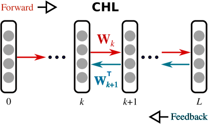
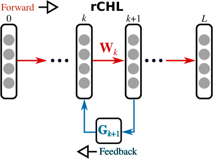
In the free phase, the input layer ${\bf x}_{0}$ is held fixed, and the signals are propagated forward through each layer (see the red arrows in figures 1). The dynamics of the neurons at each $k$-th layer are computed through the equation (1) for $k=1,\ldots,L$ (the $L+1$ layer does not exist and thus ${\bf x}_{L+1}={\bf 0}$ and ${\bf W}_{L+1}={\bf 0}$). During the clamped phase, the target signal is clamped at the output layer ${\bf x}_{L}$ and the activity of all the neurons in every layer is computed through equation (1) for $k=1,\ldots,L-1$ (notice here that the input layer $k=0$ does not express any dynamics). The backward flow is illustrated as cyan arrows in figure 1. At the end of the two phases we update the synaptic weights and the biases based on the following equations,

$$\Delta{\bf W}_{k} =\eta\gamma^{k-L}\big{(}\hat{{\bf x}}_{k}\otimes\hat{{\bf x}}_{k-1}-\check{{\bf x}}_{k}\otimes\check{{\bf x}}_{k-1}\big{)},\quad k=1,\ldots,L,$$ (2a)

$$\Delta{\bf b}_{k} =\eta\gamma^{k-L}\Big{(}\hat{{\bf x}}_{k}-\check{{\bf x}}_{k}\Big{)}$$ (2b)

where $\otimes$ is the tensor product, $\eta$ is the learning rate, $\gamma$ is the feedback gain, and $\Delta{\bf W}_{k}$ is weight update. $\check{{\bf x}}_{k}$ represents the activity of neurons in the $k$-th layer at the equilibrium configuration of equation (1) in the free phase and $\hat{{\bf x}}_{k}$ the activity of the $k$-th layer in the clamped phase.

2.2 Random Contrastive Hebbian Learning

As described by equation (1), CHL implicitly requires the synaptic weights to be symmetric (${\bf W}_{k}^{\intercal}$) in order to use the feedback information. In this work, the main contribution is to cast aside the symmetry and replace all the transpose matrices that appear in CHL with random matrices ${\bf G}_{k}$. This idea is similar to random feedback alignment [22, 35], where the error signals are propagated back through random matrices that remain constant during learning. Therefore, equation (1) is modified to the following:

$$\frac{\mathrm{d}{\bf x}_{k}}{\mathrm{d}t} =-{\bf x}_{k}+f_{k}\big{(}{\bf W}_{k}\cdot{\bf x}_{k-1}+\gamma{\bf G}_{k+1}\cdot{\bf x}_{k+1}+{\bf b}_{k}\big{)},$$ (3)

where the learning increments remain the same. In order to properly apply CHL and rCHL, we follow the second strategy of training proposed by Movellan in [31] (pg. $12$, case $2$), suggesting to first let activity settle during the clamped phase. Then, without resetting activations, free the output units and allow activity to settle again. This method assures that when the minimum for the clamped phase has been reached, it remains stable.

We summarize rCHL in Algorithm 1, where $\mathcal{I}$ is the input dataset, $\mathcal{T}$ is the corresponding target set, $N$ is the number of input samples, and $L$ is the number of layers.

$\mathcal{I}$, $\mathcal{T}$, $L$, epochs, $t_{f}$, $dt$

${\bf W}$

$N=|\mathcal{I}|$

Initialize ${\bf G}_{k}$ and ${\bf W}_{k}$ randomly for $k=1,\ldots,L$

if Bias is adaptive then

     Initialize ${\bf b}_{k}$ randomly

else

     ${\bf b}_{k}$ is fixed

end if

for $e\leftarrow 1,\ldots,\text{epochs}$ do

     $i\sim\mathcal{U}(1,N)$

     $\check{{\bf x}}_{0}=\mathcal{I}_{i}$

     $\hat{{\bf x}}_{L}=\mathcal{T}_{i}$

     for $k\leftarrow 1,\ldots,L-1$ do

         for $n\leftarrow 1,\ldots,t_{f}$ with step $dt$ do $\triangleright$ Forward Phase

              $\hat{{\bf x}}_{k}[n]=\hat{{\bf x}}_{k}[n-1]+dt\Big{(}-\hat{{\bf x}}_{k}[n-1]+f_{k}\big{(}{\bf W}_{k}\cdot\hat{{\bf x}}_{k-1}[n-1]+\gamma{\bf G}_{k+1}\cdot\hat{{\bf x}}_{k+1}[n-1]+{\bf b}_{k}\big{)}\Big{)}$

         end for

     end for

     for $k\leftarrow 1,\ldots,L$ do

         for $n\leftarrow 1,\ldots,t_{f}$ with step $dt$ do $\triangleright$ Backward Phase

              $\check{{\bf x}}_{k}[n]=\check{{\bf x}}_{k}[n-1]+dt\Big{(}-\check{{\bf x}}_{k}[n-1]+f_{k}\big{(}{\bf W}_{k}\cdot\check{{\bf x}}_{k-1}[n-1]+\gamma{\bf G}_{k+1}\cdot\check{{\bf x}}_{k+1}[n-1]+{\bf b}_{k}\big{)}\Big{)}$

         end for

     end for

     for $k\leftarrow 1,\ldots,L$ do

         ${\bf W}_{k}\leftarrow{\bf W}_{k}+\eta\gamma^{k-L}\big{(}\hat{{\bf x}}_{k}\hat{{\bf x}}_{k-1}^{\intercal}-\check{{\bf x}}_{k}\check{{\bf x}}_{k-1}^{\intercal}\big{)}$

         if Bias is adaptive then

              ${\bf b}_{k}\leftarrow{\bf b}_{k}+\eta\gamma^{k-L}\big{(}\hat{{\bf x}}_{k}-\check{{\bf x}}_{k}\big{)}$

         end if

     end for

end for

Algorithm 1 Random contrastive Hebbian learning (rCHL). $\mathcal{I}$ is the input dataset, $\mathcal{T}$ is the corresponding target set (labels) of the input data set, and $L$ is the number of layers of the network, $t_{f}$ is the simulation time and $dt$ the Forward Euler method’s time-step.

The rCHL starts with randomly initializing the synaptic weights and the feed-back random matrices. If the bias is not allowed to learn then it is fixed at the very beginning. If it’s permitted to adapt then it is randomly initialized. Then in every epoch rCHL picks up randomly an input sample and assigns it to the input layer, $\check{{\bf x}}_{0}$. At the same time, it assigns the corresponding label (target) to the output layer $\hat{{\bf x}}_{L}$. Then it solves all the non-linear coupled differential equations for each layer using a Forward Euler method for the backward phase. This means that it computes the $\hat{{\bf x}}_{k}$ and then it solves again the system of the coupled non-linear equations for the forward phase in order to compute the $\check{{\bf x}}_{k}$. Once all the activities for the forward and the backward phases have been computed, rCHL updates the synaptic weights and the biases, if they are allowed to be updated, based on equations (2)a and b.

Figure 1 illustrates the neural network architecture and the information flow of CHL (top panel) and rCHL (bottom panel). In the forward pass, the input is provided and information is propagated through matrices ${\bf W}_{k}$. In the backward phase, the output is clamped, and the information flows from the output layer to the hidden(s) through the transpose matrix ${\bf W}_{k+1}^{\intercal}$ (CHL) or random matrices ${\bf G}_{k+1}$ (rCHL).

Figure 1: Learning scheme information flow. CHL (top panel) and rCHL (lower panel) are illustrated in this figure. Both CHL and rCHL consist of two phases. In the forward phase, the input signal is fed to the network, and the activity propagates up to the deepest layer through matrices ${\bf W}_{k}$ (red arrows). In the backward phase, the output (target) signal is clamped, whilst the input signal is still present and affects the neural dynamics. The activity is propagated backwards through matrix ${\bf W}^{\intercal}_{k+1}$ (navy color arrows) in the CHL and ${\bf G}_{k+1}$ in the rCHL. It is clear that rCHL’s feedback mechanisms does not require any symmetries and acts more like a feedback system on the dynamics of neurons conveying information from the $k+1$-th layer back to $k$-th layer.

3 Results

Next, we demonstrate rCHL on a variety of tasks. The algorithm successfully solves logical operations, classification tasks and pattern generation problems. In the logical operations and classification tasks we compared our results against the state-of-the-art back-propagation (BP) and feed-back alignment (FDA). In all rCHL and CHL simulations, we used the following settings, unless otherwise stated: time step $dt=0.08$, total simulation time $t_{f}=30\mathrm{ms}$, learning rate $\eta=0.1$, and feedback gain $\gamma=0.05$.

3.1 Bars and Stripes Classification

We investigate how the parameters of the rCHL affect the learning process. In particular, we examine how to select the random matrix $\bf G$, the feedback gain $\gamma$, and the number of layers $L$. To this end we use the bars and stripes classification task to demonstrate the effect of the different parameters [23]. The dataset consists of $32$ binary images (black–$0$ and white–$1$) of size $4\times 4$ representing bars and stripes, as shown in figure 2A. We train a network of of three layers ($L=3$) with sizes $16-50-2$ to classify the input data into bars and stripes. During each epoch we pick up randomly one out of $32$ images and present it to the network for $20,000$ epochs. Every $500$ epochs we freeze the learning and we test the performance of the network. We measure the Mean Square Error (MSE) (i.e., $\frac{1}{N}\sum_{i=1}^{N}(y_{i}-\hat{y}_{i})^{2}$, where ${\bf y}$ is a reference signal of $N$ components and $\hat{{\bf y}}$ is the estimated signal) and the accuracy of the network. All neurons have sigmoid activation functions ($f_{k}(x)=\frac{1}{1+\exp(-x)}$ for all $k=1,\ldots,L$).

The achieved test MSE is shown in figure 2B and the test accuracy in figure 2C. It is apparent that rCHL converges, and the binary classification task has been learned after $5,000$ epochs. We tested two different versions of rCHL, first we used the bias terms (cyan color in figure 2) in equation (3). All ${\bf b}_{k}$ have been initialized randomly from a uniform distribution $\mathcal{U}(-0.1,0.1)$ and they are allowed to learn based on equation (2). In the second case we set the bias terms to zero (purple color in figure 2). The same method was also followed for CHL. Figures 2B and 2C indicate that CHL and rCHL can achieve similar results in the task. Once we have established the functionality of the rCHL, we investigate how the parameters of the random matrix $\bf G$, the feedback gain $\gamma$, the learning rate $\eta$, and the number of layers $L$ affect the learning.

Figure 2: Bars and stripes classification with rCHL. A Bars and stripes dataset used to train the neural network. B the test MSE computed every $500$ epochs. In every epoch, a stimulus (image) is presented to the network. Here, the rCHL algorithm (cyan and magenta curves) are compared against the CHL algorithm (black and red curves). After $5,000$ epochs the network has converged. C Test accuracy of the network on classifying the bars and stripes. We presented the entire dataset ($32$ images) during testing.

Therefore, we can conclude at that point that the rCHL has similar behavior with the CHL and the learning process works as well as CHL’s. In the following paragraphs we are investigating how four basic parameters of the model (learning rate, feed-back gain, number of layers, and the random matrix) affect the learning using the Bars and Stripes classification task as toy model. We choose to not use the bias terms since they do not affect the learning in this particular task.

3.1.1 Feedback Gain

First we start with the feedback gain by sweeping it over the interval $[0.01,1.0]$, and drawing the initial values of the synaptic weights as well as the random matrix from a uniform distribution $\mathcal{U}(-0.5,0.5)$. The effect of the feedback gain for standard CHL has been examined in [50]. In figures 3A and B, the test MSE and accuracy are shown for different values of $\gamma$. Lower feedback gain (about $0.1$), works well for rCHL. Even when the feedback gain is around $0.0001$ the learning process still works (data not shown) and the convergence is fast. This is explained by the fact that the term $\gamma^{k-L}$ in equation (2)(a) becomes extremely large for small feedback gains for the very first layers and quite small for the deeper layers. On the other hand, when when the feedback gain is high (e.g., $\gamma=1.0$) the rCHL does not converge (gray color in figure 3).

Figure 3: Effect of feedback gain $\gamma$ on bars and stripes classification. This figure illustrates the test MSE A and the test accuracy B for nine different values of feedback gain $\gamma$. Both panels illustrate that the neural network trained using the rCHL algorithm learns to classify the bars and stripes dataset in all cases, except where $\gamma=1.0$. In this case, the MSE is high and the classification is unstable.

3.1.2 Learning Rate

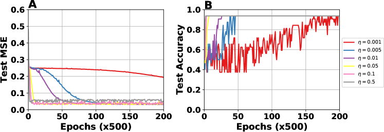
Another important parameter that affects learning is the rate the rCHL adjusts the synaptic weights, or the learning rate $\eta$. Therefore, we use the same network architecture $16-50-2$ and we keep fix the feedback gain $\gamma=0.05$ and we vary the learning rate, i.e. $\eta=\{0.001,0.005,0.01,0.05,0.1,0.5\}$. Figure 4 shows the test error and accuracy for the various values of learning rate. When the learning rate is too low the learning diverges. On the other hand when the learning rate is higher the learning converges faster. For the values between $0.005$ and $0.01$ the learning converges smoother but takes more time to reach the equilibrium in comparison to the higher values. In this case the random matrix and the synaptic weights have been initialized by a uniform distribution $\mathcal{U}(-0.5,0.5)$.

Figure 4: Effect of learning rate $\eta$ on bars and stripes classification. This figure illustrates the test MSE A and the test accuracy B for six different values of learning rate $\eta$. It is apparent that if the learning rate is too low the learning process takes more time to converge. In this case we keep the feed-back gain constant at $\gamma=0.5$.

3.1.3 Number of Layers

Next, we investigate how the number of hidden layers affects learning. To this end, we train four different neural networks using rCHL. The configurations for the networks are $16-50-2$ ($L=3$), $16-50-10-2$ ($L=4$), $16-50-20-10-2$ ($L=5$), and $16-50-30-20-10-2$ ($L=6$). As before, we draw the synaptic weights and the random matrix from a uniform distribution $\mathcal{U}(-0.5,0.5)$. Figures 5 A and B show the test MSE and test accuracy of the networks. As we increase the number of layers, the rCHL networks fail to converge (data not shown). However, when we increase the feedback gain $\gamma$, convergence is achievable (gray curves in figure 5). This behavior can be explained by the fact that the feedback gain affects the synaptic weight update by a factor $\gamma^{k-L}$. This means that the more layers a network has, the higher $\gamma$ should be.

Figure 5: Effect of number of layers $L$ on bars and stripes classification. This figure illustrates the test MSE A and the test accuracy B for four different values of $L$, which represents the number of layers. For the largest value $L=6$, rCHL diverges (data not shown) and we have to re-tune the feedback gain. Once the feedback gain has been increased, the convergence of rCHL is guaranteed (gray line).

3.1.4 Feedback Random Matrix

The random feedback matrix plays a crucial role in the rCHL learning process. It conveys the information from the output layer back to the hidden(s) one(s). Therefore, the feedback random matrix, essentially, alters the signals by applying the feedback from layer $k+1$ to neural dynamics at layer $k$. Therefore, the learning process is directly affected by the choice of the feedback random matrices within the network. The properties of random matrices arise from the distributions that generate them. In this case we investigate how random matrices generated by a normal $\mathcal{N}(0,\sigma)$ and a uniform $\mathcal{U}(a,b)$ distribution can impact the learning process. Furthermore, we define the length of the uniform distribution interval as $\ell=|b|+|a|$.

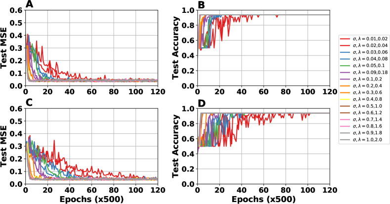
We start by varying the variance $\sigma$, and the length $\ell$ of the two different distributions. Next the network is evaluated on the bars and stripes classification task, and the MSE and accuracy are recorded. Figures 6A and B show the test MSE and accuracy, for sixteen different $\sigma$ values for the normal distribution. As shown, the higher the variance, the faster convergence is reached. Figures 6 C and D indicate the test MSE and accuracy for sixteen different values of $\ell$ of the uniform distribution. In this case, we observe that the shorter the interval (smaller $\ell$), the slower the convergence. Meanwhile, the wider the interval, the faster and the convergence is. The convergence for short intervals is slower for the uniform distribution than for corresponding small variance values for the normal distribution (see figures 6A and C).

Figure 6: Effect of matrix distribution on bars and stripes classification. This figure illustrates how the random matrix ${\bf G}_{2}$ affects the learning process when it is initialized from a normal and a uniform distribution. A Test MSE for the normal distribution, B corresponding test accuracy. C Test MSE for the uniform distribution, D corresponding test accuracy. The colored lines indicate different values for the variance $\sigma$ of the normal distribution and the interval (length $\ell$) of the uniform distribution (see the legend). The higher the variance or the length, the faster and more stable the convergence of the learning. The network with configuration $16-50-2$ performs a classification task on the bars and stripes dataset (see the text for more details).

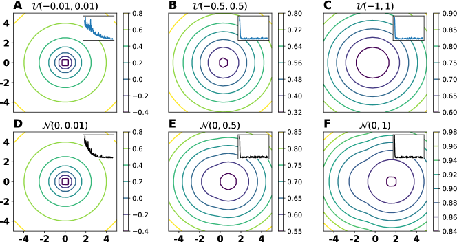
One of the key aspects in Random Matrix Theory is the spectrum (i.e., eigenvalues) of the random matrix and especially the distribution of the eigenvalues [48]. However, most connection matrices in neural networks are not square and non-normal (i.e., ${\bf V}{\bf V}^{*}\neq{\bf V}^{*}{\bf V}$, where ${\bf V}\in\mathbb{R}^{n\times n}$). Therefore, one alternative to study the spectrum of random matrices that are rectangular and non-normal is to study their singular values and the corresponding $\lambda_{\epsilon}$-pseudospectra  [46, 47, 49] (we provide a brief description of the $\lambda_{\epsilon}$-pseudospectra in the Appendix 5.1). The pseudospectra define a set of pseudoeigenvalues ($\lambda$) of a matrix ${\bf A}\in\mathbb{R}^{m\times n}$, if for some eigenvector $\boldsymbol{\upsilon}$ with $||\boldsymbol{\upsilon}||=1$ it holds $||({\bf A}-\lambda\tilde{{\bf I}})\boldsymbol{\upsilon}||\leq\epsilon$. Hence pseudospectra indicates potential sensitivity of eigenvalues under perturbations of the matrix ${\bf A}$. In this study we are interested in identifying spectral properties that can be related to the learning (i.e., convergence, speed of convergence, oscillations).

Figure 7 illustrates the $\lambda_{\epsilon}$-pseudospectra for the random matrix ${\bf G}_{2}$ for the Bars and Stripes classification task. We chose three cases for the uniform and three for the normal distribution from figure 6 and we then applied on the random matrices the algorithm given in [49] to compute the $\lambda_{\epsilon}$-pseudospectra of ${\bf G}_{2}$ in each case. In every panel the contour lines indicate the minimum singular values that correspond to different values of $\log_{10}(\epsilon)$ on the complex plane. In addition in every panel we provide the corresponding test MSE (inset plot). Subplots 7A B and C depict the pseudospectra of ${\bf G}_{2}$ drawn from uniform distributions ($\mathcal{U}(-0.01,0.01)$, $\mathcal{U}(-0.5,0.5)$, $\mathcal{U}(-1,1)$, respectively), as well as the test MSE. Likewise, subplots D, E, and F illustrate the cases of normal distributions ($\mathcal{N}(0,0.01)$, $\mathcal{N}(0,0.5)$, $\mathcal{N}(0,1)$, respectively).

Since the only varying parameter in this experiment is the way we generate the random matrix the learning process is solely affected by that matrix. Therefore, in the cases A and D the pseudospectra of the two different distributions look identical, whilst the test MSE has similar behavior, it decays slower (blue and black lines in the insets). In both cases the minimum value for $\epsilon$ is the same (and around the origin). In the other cases B, C, E, and F the convergence of the test MSE toward zero is faster (inset) and less violent (in terms of oscillations). The pseudospectra show higher minimum values for $\epsilon$. For the uniform distribution all the $\epsilon$ values are arranged on concentric circles. On the other hand, the normal distribution with variances $\sigma=0.5$ and $\sigma=1$ causes a shift towards the right-half complex plane of the pseudospectrum. The minimum $\epsilon$ is higher in comparison to the uniform cases. One more remark is that for these four cases the uniform distributions have smaller $\epsilon$ values in comparison to their normal counterparts. This might lead to a less oscillatory behavior of the test MSE as it is shown in the insets (blue and black curves). In all cases, we compute the pseudospectra using the implementation provided in [49].

Figure 7: $\Lambda_{\epsilon}$-pseudospectra of ${\bf G}_{2}$ for the Bars and Stripes classification. Six different feedback random matrices have been analyzed using the $\Lambda_{\epsilon}$-pseudospectra method. The colormap indicates the different $\epsilon$ values. The top row shows the $\Lambda_{\epsilon}$ for the matrices drawn by uniform distributions from intervals (A) $(-0.01,0.01)$, (B) $(-0.5,0.5)$, and (C) $(-1,1)$. The bottom row illustrates $\Lambda_{\epsilon}$ for the random matrices drawn from normal distributions with zero mean and variances (D) $\sigma=0.01$, (E) $\sigma=0.5$, and (F) $\sigma=1$.

3.2 Exclusive Or (XOR)

The exclusive or (denoted XOR or $\oplus$) problem consists of the evaluation of four possible Boolean input states (i.e., $1\oplus 0=1$, $1\oplus 1=0$, $0\oplus 1=1$, $0\oplus 0=0$). To solve the XOR problem, we use a feed-forward network with one hidden layer and one output layer ($L=3$) with a configuration $2-2-1$. All neural units are sigmoidal: $f(x)=(1+\exp(-x))^{-1}$, and we train the neural network on the XOR problem for $5,000$ epochs using CHL and rCHL. The random matrix $\bf G$ for rCHL has been initialized from a uniform distribution $\mathcal{U}(-0.2,0.2)$. In every epoch we present $128$ samples to the network and every $500$ epochs we measure the MSE and the accuracy on the test dataset. The accuracy here is defined to be $\frac{1}{4}\sum_{i=1}^{4}|x_{2}(t)-T_{i}|<\epsilon$, where $\epsilon=0.01$ and the index $i$ runs over the test samples.

Figure 8: Exclusive OR (XOR). Four different learning algorithms have been use to train a feed-forward network with three layers, $L=3$, ($2-2-1$). (A) Test MSE error illustrated against the number of samples, (B) test accuracy. The red and purples lines indicate the CHL and rCHL, respectively. The brown and gray dashed lines show the minimum test MSE and the maximum test accuracy for the BP and the FDA, respectively.

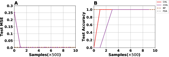
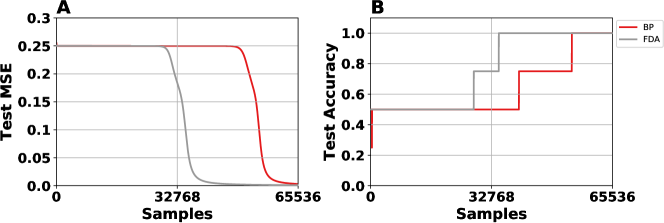
The results of the learning are shown in figure 8, where figure 8A shows the test error, and figure 8B the test accuracy for CHL (red line) and rCHL (purple line). The test error and the test accuracy attained is the same for BP (brown dashed line) and FDA (gray dashed line). Comparing against the error and accuracy of BP and FDA (see SI figure 11), rCHL converges faster and more smoothly. This is because rCHL and CHL are on-line learning algorithms, and the input and target signals are both embedded into the dynamics of the neurons. This leads to a rapid convergence of the Hebbian learning rule, which rapidly assimilates the proper associations between input and output signals.

3.3 Handwritten Digit and Letter Classification

For the classification tasks, we used the MNIST [7] dataset of $10$ handwritten digits and the eMNIST datasets [5] of $26$ handwritten letters of the English alphabet. The neural network layouts for the MNIST and the eMNIST was $784-128-64-10$ and $784-256-128-26$, respectively. On every unit in both MNIST and eMNIST networks, we use a sigmoid function: $f(x)=(1+\exp(-x))^{-1}$. We drew the initial synaptic weights and the random matrices from uniform distributions $\mathcal{U}(-0.6,0.6)$ and $\mathcal{U}(-0.3,0.3)$, respectively. We trained the network for $20$ (MNIST) and $40$ (eMNIST) epochs, and in each epoch we present the entire MNIST and eMNIST datasets, which consist of $60,000$ and $124,800$ images, respectively. At the end of each epoch, we measured the MSE and the accuracy of the network. The accuracy is defined to be the ratio of the successfully classified images to the total presented test images ($10,000$ for MNIST and $20,800$ for eMNIST, respectively).

Figure 9: MNIST and eMNIST digits classification. The figure illustrates  (A) the test error and (B) the accuracy of a neural network ($784-128-64-10$) with sigmoid function as non-linearity in all layers. The network was trained on the entire MNIST set of digits ($50,000$ images) and tested on the whole MNIST test set ($10,000$ images). In addition, (C) illustrates the test error and (D) the accuracy of a neural network ($784-256-128-26$) with sigmoid function as non-linearity in all layers. The network was trained on the entire eMNIST set of digits ($124,800$ images) and tested on the whole eMNIST test set ($20,800$ images). In both cases the MNIST and the eMNIST, CHL and rCHL have similar performance (red and purple curves, respectively).

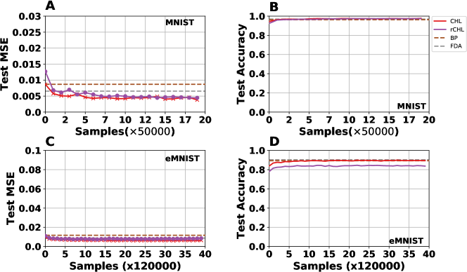
Figure 9A illustrates the test error of CHL (red line) and rCHL (purple line), respectively. The error is lower than BP and FDA (brown and gray dashed lines, respectively), and the convergence is faster (compared against SI figure 12, where BP and FDA test MSE and accuracy are illustrated). However, the classification test accuracy is the same as for BP and FDA, as figure 9B indicates. The convergence of the BP and FDA algorithms can be seen in SI figure 12, as well as the test accuracy of those algorithms performing on the same type of neural network (same neural units and network architecture).

For the eMNIST dataset, the test error is illustrated in figure 9C, where the error of CHL (red line) and rCHL (purple line) are close to the error attained by BP and FDA (brown and gray dashed lines). However, the classification test accuracy of rCHL is worse than the other three learning algorithms (CHL, BP and FDA), as figures 9D and SI 13 B show. For the eMNIST data set the accuracy of the rCHL is lower than the other three algorithms despite the fact that the error is smaller than the errors of BP and FDA. This drawback might be due to the feed-back random matrix and the lack of symmetric synaptic connections. This is also supported by the fact that the CHL (which differs from rCHL only in the way the feedback signals are transmitted) achieves an accuracy as good as the BP and FDA (minimum test error and maximum test accuracy for all four algorithms are provided in table 1,Appendix 5.2).

3.4 Autoencoder

The final test case was the implementation of an autoencoder using CHL and rCHL. An autoencoder is a neural network that learns to reconstruct the input data using a restricted latent representation. Classic autoencoders consist of three layers: the first layer is called the encoder, which is responsible for encoding the input data to the hidden layer, which describes a code. The third layer is the decoder, which generates the approximation of the input data, based on the code provided by the hidden layer [12].

To this end, we use a network with three layers $L=3$, with a layout $784-36-784$, and we use the MNIST handwritten digits. This means that we encode the input images of dimension $784$ to a dimension of $36$. For both CHL and rCHL, the learning rate is set to $\eta=0.05$. The synaptic weights and the random matrix ${\bf G}$ were initialized from uniform distributions $\mathcal{U}(-0.5,0.5)$ and $\mathcal{U}(-1,1)$, respectively. We trained the network for $20$ epochs, and in each epoch we presented to the network $5,000$ samples of MNIST handwritten digits.

Figure 10: CHL and rCHL autoencoder. The MNIST dataset was used to train an autoencoder using CHL and rCHL. (A) shows some randomly chosen MNIST digits. After training the network for $40$ epochs (during each epoch we presented $5,000$ MNIST images to the network), it was able to reconstruct the learned digits as panel (B) shows for CHL, and panel (C) for rCHL. The learned representations are shown in panels (D) and (E) for CHL and rCHL, respectively.

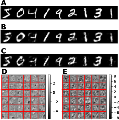
After training the autoencoder, we fed $9$ digits (figure 10A) from the MNIST dataset to the autoencoders. The decoding (reconstruction) of the input data is illustrated in figures 10B and 10C for CHL and rCHL, respectively. The results indicate that rCHL and its non-random counterpart (CHL), can both learn to approximate the identity function, and thus they are both good candidates for implementing autoencoders. The reconstruction (decoding) was not perfect, which implies that the network correctly learned an approximation (and not the exact function), indicating that the network had learned the appropriate representations (code). The representations (codebooks) are shown in figures 10D and 10E for the CHL and rCHL models, respectively. As expected, the representations of rCHL were more noisy than that of the CHL model. This can be partially explained by the chosen simulation parameters in this experiment.

4 Discussion

In this work, we introduced a modified version of Contrastive Hebbian Learning  [50, 31, 3], based on random feedback connections. The key contribution of this work is a biologically plausible variant of CHL, attained by using random fixed matrices (during learning) instead of bidirectional synapses. We have shown that this new variation of CHL, random Contrastive Hebbian Learning, can achieve results equivalent to that of CHL, BP, or FDA. In addition, rCHL can solve logical problems such as the XOR, as well as classification tasks, such as the handwritten digits and letters classification (MNIST and eMNIST datasets). Furthermore, rCHL supports representation learning (e.g., autoencoders), as well.

We provide a thorough investigation of the algorithm, examining how the different parameters of the learning scheme affect the learning process. We have shown that the feedback gain $\gamma$ affects the performance of learning. The smaller the gain $\gamma$, the better the performance of the algorithm, implying that the feedback gain should be small. This is in accordance with previous theoretical results found in [50], where CHL requires low values of $\gamma$ in order to be equivalent to BP. A second factor that affects learning is the number of hidden layers. When the number of hidden layers increases, the performance of the learning decreases. However, this can be mitigated by increasing the feedback gain $\gamma$ (see figure 5). Finally, we tested the initial conditions of the random matrix ${\bf G}$. We found that if we choose the random matrix from a normal distribution with zero mean, the convergence speed of the learning algorithm is faster than if we draw ${\bf G}$ from a uniform distribution. In addition, the variance $\sigma$ and the interval length $\lambda$ of the normal and uniform distributions, respectively, affect the learning as well. The smaller the values, the faster the convergence of the learning.

We further investigated the feedback random matrices using tools provided by the pseudospectra analysis [46, 49]. The convergence of learning can be affected by the choice of distribution that generates the feedback random matrix. We found that sub-Gaussian feedback matrices with normal-like pseudospectrum tend to cause slower convergence of learning, but a more robust one. On the other hand, Gaussian random matrices tend to have faster convergence.

Both CHL and rCHL share some common properties such as (i) the neurons express non-linear dynamics, (ii) the learning rule is based on Hebb’s rule [14], which means no biologically implausible information is necessary (e.g., knowledge of the derivatives of the non-linearities of the neural units), (iii) the propagation of the activity from one layer to the next takes place in a manner similar that of biological systems. All the layers are coupled through a non-linear dynamical system, which implies that when an input is presented the algorithm does not have to wait until all the units in the $k$-th layer have fired. Instead, neurons can propagate their activity through couplings to the next $(k+1)$-th layer. This is not the case for artificial neural networks where the activity is computed for all the units of the $k$-th layer prior to transmission to the subsequent layer. Thus, CHL and rCHL circulate signals in a more natural fashion (similar to the processes evident in biological nervous systems).

The salient difference between CHL and rCHL is the replacement of symmetric synaptic weights (CHL) with fixed random matrices (rCHL). Therefore, the feedback connections do not require any symmetric weights (transpose matrices) of the feed-forward connections. This is in accordance with biology since there is no evidence thus far to indicate that chemical synapses (one of the two major synapse types in the nervous system, the other being electrical synapses) are bidirectional [17, 40]. More precisely, we can interpret the random feedback as a model of afferent feedback connections from higher hierarchical layers to lower ones. For instance, primary sensory areas are connected in series with higher sensory or multi-modal areas. These higher areas project back to the primary areas through feedback pathways [26, 36, 11]. Other types of feedback pathways to which our approach may be considered relevant are the inter-laminar connections within cortical layers [13, 45]. Therefore, such feedback pathways can be modeled as random feedback matrices that interfere with the neural dynamics of the lower layers (top-down signal transmission). The randomness in these feedback pathways can account for currently unknown underlying neural dynamics or random networks with interesting properties [29, 48].

Our current implementation, rCHL, allows us to interpret the backward phase (clamped) as a top-down signal propagation. For instance, when a visual stimulus is presented, such as a letter, and a subject is required to learn the semantic of the letter (which letter is presented), then the target can be the semantic and the input signal the image of the letter. Therefore, we can assume that the forward phase simulates the bottom-up signal propagation from the primary sensory cortices to higher associate cortices, and the backward phase as the top-down signal propagation from the higher cognitive areas back to the lower cortical areas.

Due to the nature of the learning algorithm and the two phases (positive and negative), the input and the target signals are clamped, and the dynamics of those signals are captured and embedded in the neural dynamics of the network. This can be compared to target propagation [21, 19], where the loss gradient of BP is replaced by a target value. When the target value is very close to the neural activation of the forward pass, TP behaves like BP. These sort of learning algorithms solve the credit assignment problem [30], using local information. In the proposed model, the target and the input signals are both embedded into the dynamics of the neural activity and affect the learning process in an indirect way through a Hebb and an anti-Hebb rule.

The major contribution of this work is the development of a new method to implement CHL using random feedback instead of symmetric one. This leads to a more biologically plausible implementation of CHL without loss of performance and accuracy in most of the cases studied. In addition, the algorithm offers a shorter runtime since it does not require the computation of the transpose matrix for synaptic weights at every time step. Furthermore, the proposed algorithm offers a suitable learning scheme for neuromorphic devices since its neural dynamics can be transformed into spiking neurons [10]. Therefore, we can build spiking neural networks with STDP-like learning rules as equivalent to the Hebb’s rule in rCHL and use ideas from event-based Contrastive Divergence [32] and synaptic sampling machines [34] in order to implement a neuromorphic rCHL. This idea is similar to the event-based random back-propagation algorithm [33], where the authors have implemented an event-based feedback alignment equivalent for neuromorphic devices.

A potential extension of the model might be a replacement of the firing rate units with spiking neurons, such as leaky integrate-and-fire units, in order to make the computations even more similar to the biological case. Another potential direction would be to remove entirely the synchronization in the neural dynamics integration. This means that the integrations of neural dynamics can take place on-demand in a more event-based fashion [41, 44]. Since the units are coupled with each other, and the propagation of activity takes place in a more natural way, we might be able to use asynchronous algorithms for implementing rCHL such that it scales up in a more efficient and natural way. Another extension of the model in the future would be to impose sparsity constraints on the learning rule in order to render data encoding processes more efficient. Furthermore, such a modification would make the model able to simulate more biological phenomena, such as the sparse compression occurring within the hippocampus [39].

In the future, we would like to conduct more analytical work to determine the optimal type of random matrix ${\bf G}$, for a given problem, and how to design such a matrix, if it does exist. This means that if an optimal random matrix ${\bf G}$ exists, then one can properly choose the eigenvalues (or singular values) and the distribution that generates that matrix based on the problem they would like to solve. To this end, the pseudospectra analysis can play a key role. Pseudospectra can help us to better understand the relations between singular values, convergence of learning and accuracy. This can lead to the development of sophisticated methods for designing feedback matrices with particular properties. Therefore, we could improve and accelerate the learning process.

Author Contributions

GD conceived the idea, implemented CHL and rCHL, ran the CHL and rCHL experiments; TB implemented and ran the BP and FDA experiments; GD analyzed and interpreted the results; All the authors wrote and reviewed the manuscript.

Acknowledgments

This work was supported in part by the Intel Corporation and by the National Science Foundation under grant 1640081. We thank NVIDIA corporation for providing the GPU used in this work.

5 Appendix

5.1 $\Lambda_{\epsilon}$-pseudospectra

Let ${\bf V}\in\mathbb{R}^{m\times n}$ be a rectangular matrix, not necessarily normal (i.e., ${\bf V}{\bf V}^{*}\neq{\bf V}^{*}{\bf V}$). The $\epsilon$-pseudospectra ($\Lambda_{\epsilon}$) [47, 49] is the set of $\epsilon$-eigenvalues a closed subset of $\mathbb{C}$.

Definition 5.1 ($\epsilon$-Pseudospectra).

Let ${\bf V}\in\mathbb{C}\text{ or }\mathbb{R}$, $z\in\mathbb{C}$ and $\tilde{{\bf I}}\in\mathbb{R}^{m\times n}$ (the identity matrix with ones on the main diagonal and zeros elsewhere), then the $\epsilon$-pseudospectra $\Lambda_{\epsilon}=\{z\in\mathbb{C}:||({\bf V}-z\tilde{{\bf I}}){\boldsymbol{\upsilon}}||\leq\epsilon\text{ for some }\boldsymbol{\upsilon}\in\mathbb{C}^{n},||\boldsymbol{\upsilon}||=1\}$.

Definition 5.2 ($\epsilon$-Pseudospectra).

Let ${\bf V}\in\mathbb{C}\text{ or }\mathbb{R}$, $z\in\mathbb{C}$ and $\tilde{{\bf I}}\in\mathbb{R}^{m\times n}$ (the identity matrix with ones on the main diagonal and zeros elsewhere), then the $\epsilon$-pseudospectra $\Lambda_{\epsilon}=\{z\in\mathbb{C}:\sigma_{\min}(z\tilde{{\bf I}}-{\bf V})\leq\epsilon\}$.

Definitions 5.1 and 5.2 are equivalent [49], and both account for the computation of $\Lambda_{\epsilon}$ of rectangular matrices of dimension $m\times n$, where $m\geq n$. The algorithm given in [49] for the numerical computation of the set $\Lambda_{\epsilon}$ can be applied on matrices of dimension $m\times n$, where either $m\geq 2n$ or $m\leq 2n$.

5.2 Error and Accuracy Table

Here we provide the minimum test error and maximum test accuracy for each of the experiments (XOR, MNIST and eMNIST). We compare in the following table our CHL and rCHL implementations against each other and against the BP and the FDA.

	XOR	MNIST	eMNIST
BP	$0.003/1$	$0.0087/0.962$	$0.0116/0.8935$
FDA	$0.0009/1$	$0.0066/0.969$	$0.0087/0.9035$
CHL	${2.503}\mathrm{e}{-8}/1$	$0.0038/0.977$	$0.0061/0.899$
rCHL	${\bf{1.117}\mathrm{e}{-6}/1}$	${\bf 0.0044/0.975}$	${\bf 0.0073/0.8461}$

Table 1: Mean squared error (MSE) and Accuracy. The test MSE and accuracy of three experiments, XOR, MNIST, and eMNIST are given in this table. BP–Backpropagation, FDA–Feedback Alignment, CHL– Contrastive Hebbian Learning, and rCHL–random Contrastive Hebbian Learning.

5.3 Abbreviations and Notation Tables

Abbreviation	Description
STDP	Spike-timing Dependent Plasticity
BP	Back-propagation
FDA	Feedback Alignment
CHL	Contrastive Hebbian Learning
rCHL	random Contrastive Hebbian Learning
MSE	Mean Squared Error

Table 2: Abbreviations

Symbols	Description
$L$	Total number of layers
$k$	Index of layer
${\bf x}_{k}$	Neural state at layer $k$
$\check{{\bf x}}_{k}$	Neural state at layer $k$ in the free phase
$\hat{{\bf x}}_{k}$	Neural state at layer $k$ in the clamped phase
${\bf W}_{k}$	Synaptic matrix (connects layer $k-1$ with $k$)
${\bf G}_{k}$	Random feedback matrix (connects layer $k-1$ with $k$
${\bf b}_{k}$	Bias for layer $k$
$f_{k}$	Non-linear function (transfer function)
$\eta$	Learning rate
$\gamma$	Feedback gain
$\otimes$	Tensor product
$dt$	Forward Euler time-step
$t_{f}$	Forward Euler total integration time
$\mathcal{I}$	Input data set
$\mathcal{T}$	Target set
$\Lambda_{\epsilon}$	Set of pseudospectra
$\lambda$	Eigenvalue
$\mathcal{U}$	Uniform distribution
$\ell$	Length of uniform’s distribution interval
$\mathcal{N}$	Normal distribution
$\sigma$	Normal distribution’s variance
$\oplus$	Exclusive Or (XOR)

Table 3: Notation

5.4 Simulation and Platform Details

All serial simulations were run on a Dell OptiPlex $7040$ with $16$GB physical memory, and a $6$th generation Intel i$7$ processor (Intel(R) Core(TM) i7-6700 CPU @ 3.40GHz) running Arch Linux ($4.11.9-1$-ARCH $\times 86\_64$ GNU/Linux). The source code for CHL and rCHL were written in the C programming language [18] (gcc (GCC) $7.1.120170630$). In all C simulations, we used the random number generator provided by [37]. The backpropagation and feedback alignment algorithms were written in Python using Tensorflow [1], and ran on an Nvidia GeForce GTX Titan X with $12\,\mathrm{GB}$ memory. The source code is distributed under the GNU General Public License, and can be found at: [LINK]. All simulation parameters are provided in the Results section and in the Supplementary Information (SI).

5.5 Simulation Parameters

Experiment	$\eta$	$\gamma$	Epochs	Layout	${\bf G}_{k}$	${\bf W}_{k}^{0}$	${\bf b}_{k}^{0}$
XOR	$0.1$	$0.05$	$5,000$	$(2,2,1)$	$\mathcal{U}(-0.2,0.2)$	$\mathcal{U}(0,1)$	$-$
MNIST	$0.1$	$0.05$	$20$	$(784,128,64,10)$	$\mathcal{U}(-0.6,0.6)$	$\mathcal{U}(-0.5,0.5)$	$-$
eMNIST	$0.1$	$0.1$	$40$	$(784,256,128,26)$	$\mathcal{U}(-0.3,0.3)$	$\mathcal{U}(-0.5,0.5)$	$\mathcal{U}(-0.2,0.2)$
Autoencoder	$0.05$	$0.05$	$20$	$(784,36,784)$	$\mathcal{U}(-1,1)$	$\mathcal{U}(-0.5,0.5)$	$-$

Table 4: Simulation Parameters. In the experiments, we integrated the dynamics for $t_{f}=30\,\mathrm{ms}$ using the forward Euler method with time-step $dt=0.08$. $\eta$ is the learning rate and $\gamma$ is the feedback gain.

Supplementary Information

Backpropagation and Feedback Alignment on XOR

Figure 11: Backpropagation (BP) and feedback alignment (FDA) on XOR. The test MSE (A) and the test accuracy (B) show the convergence of BP (red) and FDA (gray) in solving the XOR problem. For training both BP and FDA, we used $65,536$ batches, and each batch had a size of $1$ sample. The learning rate was $\eta=0.1$ and the momentum $\alpha=0.1$. Synaptic weights and biases were initialized using uniform distributions $\mathcal{U}(-0.3,0.3)$ and $\mathcal{U}(-0.1,0.1)$, respectively.

Backpropagation and Feedback Alignment on MNIST

Figure 12: Backpropagation (BP) and feedback alignment (FDA) on MNIST. The test MSE (A) and the test accuracy (B) show the convergence of BP (red) and FDA (gray) in solving MNIST handwritten digits classification problem. For training both BP and FDA, we used $524,288$ batches, and each batch had a size of $128$ samples. The learning rate was $\eta=0.07$. Synaptic weights and biases were initialized using uniform distributions $\mathcal{U}(-0.3,0.3)$ and $\mathcal{U}(-0.1,0.1)$, respectively.

Backpropagation and Feedback Alignment on eMNIST

Figure 13: Backpropagation (BP) and feedback alignment (FDA) on eMNIST. The test MSE (A) and the test accuracy (B) show the convergence of BP (red) and FDA (gray) in solving the eMNIST handwritten letters classification problem ($26$ letters of the English alphabet). For training both BP and FDA, we used $1,048,576$ batches, and each batch had size of $128$ samples. The learning rate was $\eta=0.07$. Synaptic weights and biases were initialized using uniform distributions $\mathcal{U}(-0.3,0.3)$ and $\mathcal{U}(-0.1,0.1)$, respectively.

References

- [1] Martín Abadi, Paul Barham, Jianmin Chen, Zhifeng Chen, Andy Davis, Jeffrey Dean, Matthieu Devin, Sanjay Ghemawat, Geoffrey Irving, Michael Isard, et al. Tensorflow: A system for large-scale machine learning. In OSDI, volume 16, pages 265–283, 2016.
- [2] Larry F Abbott and Sacha B Nelson. Synaptic plasticity: taming the beast. Nature neuroscience, 3(11s):1178, 2000.
- [3] Pierre Baldi and Fernando Pineda. Contrastive learning and neural oscillations. Neural Computation, 3(4):526–545, 1991.
- [4] Guo-qiang Bi and Mu-ming Poo. Synaptic modifications in cultured hippocampal neurons: dependence on spike timing, synaptic strength, and postsynaptic cell type. Journal of neuroscience, 18(24):10464–10472, 1998.
- [5] Gregory Cohen, Saeed Afshar, Jonathan Tapson, and André van Schaik. Emnist: an extension of mnist to handwritten letters. arXiv preprint arXiv:1702.05373, 2017.
- [6] Steven J Cooper. Donald o. hebb’s synapse and learning rule: a history and commentary. Neuroscience & Biobehavioral Reviews, 28(8):851–874, 2005.
- [7] Li Deng. The mnist database of handwritten digit images for machine learning research [best of the web]. IEEE Signal Processing Magazine, 29(6):141–142, 2012.
- [8] Stuart Dreyfus. The numerical solution of variational problems. Journal of Mathematical Analysis and Applications, 5(1):30–45, 1962.
- [9] Nels C Elde, Stephanie J Child, Michael T Eickbush, Jacob O Kitzman, Kelsey S Rogers, Jay Shendure, Adam P Geballe, and Harmit S Malik. Poxviruses deploy genomic accordions to adapt rapidly against host antiviral defenses. Cell, 150(4):831–841, 2012.
- [10] Wulfram Gerstner and Werner M Kistler. Spiking neuron models: Single neurons, populations, plasticity. Cambridge university press, 2002.
- [11] Matthew F Glasser, Timothy S Coalson, Emma C Robinson, Carl D Hacker, John Harwell, Essa Yacoub, Kamil Ugurbil, Jesper Andersson, Christian F Beckmann, Mark Jenkinson, et al. A multi-modal parcellation of human cerebral cortex. Nature, 536(7615):171–178, 2016.
- [12] Ian Goodfellow, Yoshua Bengio, and Aaron Courville. Deep Learning. MIT Press, 2016.
- [13] Kenneth D Harris and Thomas D Mrsic-Flogel. Cortical connectivity and sensory coding. Nature, 503(7474):51, 2013.
- [14] Donald Olding Hebb. The organization of behavior: A neuropsychological theory. Psychology Press, 2005.
- [15] Geoffrey E Hinton. Training products of experts by minimizing contrastive divergence. Neural computation, 14(8):1771–1800, 2002.
- [16] Geoffrey E Hinton and James L McClelland. Learning representations by recirculation. In Neural information processing systems, pages 358–366, 1988.
- [17] Eric R Kandel, James H Schwartz, Thomas M Jessell, Steven A Siegelbaum, A James Hudspeth, et al. Principles of neural science, volume 4. McGraw-hill New York, 2000.
- [18] Brian W Kernighan and Dennis M Ritchie. The C programming language. 2006.
- [19] Yann Le Cun. Learning process in an asymmetric threshold network. In Disordered systems and biological organization, pages 233–240. Springer, 1986.
- [20] Yann LeCun, Yoshua Bengio, and Geoffrey Hinton. Deep learning. nature, 521(7553):436, 2015.
- [21] Dong-Hyun Lee, Saizheng Zhang, Asja Fischer, and Yoshua Bengio. Difference target propagation. In Joint european conference on machine learning and knowledge discovery in databases, pages 498–515. Springer, 2015.
- [22] Timothy P Lillicrap, Daniel Cownden, Douglas B Tweed, and Colin J Akerman. Random synaptic feedback weights support error backpropagation for deep learning. Nature communications, 7, 2016.
- [23] David JC MacKay. Information theory, inference, and learning algorithms, volume 7. Citeseer, 2003.
- [24] Stephen L Macknik and Susana Martinez-Conde. The role of feedback in visual masking and visual processing. Advances in cognitive psychology, 2007.
- [25] Stephen L Macknik and Susana Martinez-Conde. The role of feedback in visual attention and awareness. Cognitive Neurosciences, 1, 2009.
- [26] Nikola T Markov, MM Ercsey-Ravasz, AR Ribeiro Gomes, Camille Lamy, Loic Magrou, Julien Vezoli, P Misery, A Falchier, R Quilodran, MA Gariel, et al. A weighted and directed interareal connectivity matrix for macaque cerebral cortex. Cerebral cortex, 24(1):17–36, 2012.
- [27] Nikola T Markov, Julien Vezoli, Pascal Chameau, Arnaud Falchier, René Quilodran, Cyril Huissoud, Camille Lamy, Pierre Misery, Pascale Giroud, Shimon Ullman, et al. Anatomy of hierarchy: feedforward and feedback pathways in macaque visual cortex. Journal of Comparative Neurology, 522(1):225–259, 2014.
- [28] Henry Markram, Joachim Lübke, Michael Frotscher, and Bert Sakmann. Regulation of synaptic efficacy by coincidence of postsynaptic aps and epsps. Science, 275(5297):213–215, 1997.
- [29] Robert M May. Simple mathematical models with very complicated dynamics. Nature, 261(5560):459, 1976.
- [30] Marvin Minsky. Steps toward artificial intelligence. Proceedings of the IRE, 49(1):8–30, 1961.
- [31] Javier R Movellan. Contrastive hebbian learning in the continuous hopfield model. In Connectionist models: Proceedings of the 1990 summer school, pages 10–17, 1991.
- [32] Emre Neftci, Srinjoy Das, Bruno Pedroni, Kenneth Kreutz-Delgado, and Gert Cauwenberghs. Event-driven contrastive divergence for spiking neuromorphic systems. Frontiers in neuroscience, 7:272, 2014.
- [33] Emre O Neftci, Charles Augustine, Somnath Paul, and Georgios Detorakis. Event-driven random back-propagation: Enabling neuromorphic deep learning machines. Frontiers in neuroscience, 11, 2017.
- [34] Emre O Neftci, Bruno U Pedroni, Siddharth Joshi, Maruan Al-Shedivat, and Gert Cauwenberghs. Stochastic synapses enable efficient brain-inspired learning machines. Frontiers in neuroscience, 10:241, 2016.
- [35] Arild Nøkland. Direct feedback alignment provides learning in deep neural networks. In Advances in Neural Information Processing Systems, pages 1037–1045, 2016.
- [36] Seung Wook Oh, Julie A Harris, Lydia Ng, Brent Winslow, Nicholas Cain, Stefan Mihalas, Quanxin Wang, Chris Lau, Leonard Kuan, Alex M Henry, et al. A mesoscale connectome of the mouse brain. Nature, 508(7495):207, 2014.
- [37] Melissa E. O’Neill. Pcg: A family of simple fast space-efficient statistically good algorithms for random number generation. Technical Report HMC-CS-2014-0905, Harvey Mudd College, Claremont, CA, September 2014.
- [38] Randall C O’Reilly. Biologically plausible error-driven learning using local activation differences: The generalized recirculation algorithm. Neural computation, 8(5):895–938, 1996.
- [39] Panagiotis C Petrantonakis and Panayiota Poirazi. A compressed sensing perspective of hippocampal function. Frontiers in systems neuroscience, 8, 2014.
- [40] Virginia M Pickel and Menahem Segal. The synapse: structure and function. Elsevier, 2013.
- [41] Nicolas P Rougier and Axel Hutt. Synchronous and asynchronous evaluation of dynamic neural fields. Journal of Difference Equations and Applications, 17(8):1119–1133, 2011.
- [42] David E Rumelhart, Geoffrey E Hinton, Ronald J Williams, et al. Learning representations by back-propagating errors. Cognitive modeling, 5(3):1, 1988.
- [43] Tian-De Shou. The functional roles of feedback projections in the visual system. Neuroscience bulletin, 26(5):401–410, 2010.
- [44] Wahiba Taouali, Frédéric Alexandre, Axel Hutt, and Nicolas P Rougier. Asynchronous evaluation as an efficient and natural way to compute neural networks. In AIP Conference Proceedings, volume 1168, pages 554–558. AIP, 2009.
- [45] Alex M Thomson and A Peter Bannister. Interlaminar connections in the neocortex. Cerebral cortex, 13(1):5–14, 2003.
- [46] Lloyd N Trefethen. Pseudospectra of matrices. Numerical analysis, 91:234–266, 1991.
- [47] Lloyd N Trefethen and Mark Embree. Spectra and pseudospectra: the behavior of nonnormal matrices and operators. Princeton University Press, 2005.
- [48] Van H Vu. Modern Aspects of Random Matrix Theory, volume 72. American Mathematical Society, 2014.
- [49] Thomas G Wright and Lloyd N Trefethen. Pseudospectra of rectangular matrices. IMA Journal of Numerical Analysis, 22(4):501–519, 2002.
- [50] Xiaohui Xie and H Sebastian Seung. Equivalence of backpropagation and contrastive hebbian learning in a layered network. Neural computation, 15(2):441–454, 2003.
- [51] Li I Zhang, Huizhong W Tao, Christine E Holt, William A Harris, and Mu-ming Poo. A critical window for cooperation and competition among developing retinotectal synapses. Nature, 395(6697):37, 1998.