Fornax: a Flexible Code for Multiphysics Astrophysical Simulations

M. Aaron Skinner11affiliation: Livermore National Laboratory, 7000 East Ave., Livermore, CA 94550-9234; skinner15@llnl.gov Joshua C. Dolence22affiliation: CCS-2, Los Alamos National Laboratory, P.O. Box 1663, Los Alamos, NM 87545; jdolence@lanl.gov Adam Burrows33affiliation: Department of Astrophysical Sciences, Princeton University, Princeton NJ 08544; burrows@astro.princeton.edu,dvartany@astro.princeton.edu David Radice33affiliation: Department of Astrophysical Sciences, Princeton University, Princeton NJ 08544; burrows@astro.princeton.edu,dvartany@astro.princeton.edu 44affiliation: Schmidt Fellow, Institute for Advanced Study, 1 Einstein Drive, Princeton, NJ 08540; dradice@astro.princeton.edu David Vartanyan33affiliation: Department of Astrophysical Sciences, Princeton University, Princeton NJ 08544; burrows@astro.princeton.edu,dvartany@astro.princeton.edu
Abstract

This paper describes the design and implementation of our new multi-group, multi-dimensional radiation hydrodynamics (RHD) code Fornax and provides a suite of code tests to validate its application in a wide range of physical regimes. Instead of focusing exclusively on tests of neutrino radiation hydrodynamics relevant to the core-collapse supernova problem for which Fornax is primarily intended, we present here classical and rigorous demonstrations of code performance relevant to a broad range of multi-dimensional hydrodynamic and multi-group radiation hydrodynamic problems. Our code solves the comoving-frame radiation moment equations using the M1𝑀1M1 closure, utilizes conservative high-order reconstruction, employs semi-explicit matter and radiation transport via a high-order time stepping scheme, and is suitable for application to a wide range of astrophysical problems. To this end, we first describe the philosophy, algorithms, and methodologies of Fornax and then perform numerous stringent code tests, that collectively and vigorously exercise the code, demonstrate the excellent numerical fidelity with which it captures the many physical effects of radiation hydrodynamics, and show excellent strong scaling well above 100k MPI tasks.

Subject headings:
methods: numerical
slugcomment: Received June 19, 2018; Accepted January 20, 2019

1. Introduction

In recent years, there has been an explosion of techniques and codes to solve the equations of radiation hydrodynamics in astrophysical environments (Hubeny & Burrows 2007; Krumholz et al. 2007; Swesty & Myra 2009; Stone et al. 2008; Marek & Janka 2009; Vaytet et al. 2011; Müller, Janka, & Dimmelmeier 2010; Shibata et al. 2011; Kuroda, Kotake, & Takiwaki 2012; Zhang et al. 2011,2013; Davis et al. 2012; Ott et al. 2012,2013; Kolb et al. 2013; Couch 2013; Couch & O’Connor 2014; Teyssier 2015; Roberts et al. 2016; Bruenn et al. 2016; Nagakura et al. 2018; O’Connor & Couch 2018). To address a broad class of radiation hydrodynamics problems, we have recently developed an entirely new multi-dimensional, multi-group radiation hydrodynamic code, Fornax, primarily, but not exclusively, to study core-collapse supernovae (Skinner, Burrows, & Dolence 2016; Radice et al. 2017; Burrows et al. 2018; Vartanyan et al. 2018). However, to keep this paper manageable and focused, we reserve for a later paper the explicit tests of the specifically neutrino radiation hydrodynamics of relevance in the core-collapse supernovae problem and focus on tests relevant to generic radiation-hydrodynamic problems.

Most of Fornax is written in C, with only a few Fortran 95 routines for reading in microphysical data tables, and we use an MPI/OpenMP hybrid parallelism model now optimized for Cray and KNL architectures. Fornax employs general orthogonal coordinates in one, two, and three spatial dimensions, solves the comoving-frame, multi-group, two-moment, velocity-dependent transport equations to 𝒪(v/c)𝒪𝑣𝑐\mathcal{O}(v/c), and uses the M1𝑀1M1 tensor closure for the second and third moments of the radiation fields (Dubroca & Feugeas 1999; Vaytet et al. 2011). Fornax can accommodate any orthogonal geometry, though for the core-collapse supernova (CCSN) problem we generally employ a spherical grid. In this paper, we describe in detail the computational philosophy and methods of Fornax2), the formulation of the equations (§3), the discretization approach (§4), specifics concerning reconstruction, solvers, and coupling (§5), the algorithmic steps (§6), the implementation details of the dendritic grid in 3-d spherical coordinates (§7), the results of numerous standard hydrodynamic (§8) and radiation (§9) test problems, and conclude with some general observations in §10.

2. General Description of Fornax

The hydrodynamics in Fornax is based on a directionally-unsplit, Godunov-type finite-volume method. Fluxes at cell faces are computed with the fast and accurate HLLC approximate Riemann solver based on left and right states reconstructed from the underlying volume-averages. The reconstruction is accomplished via a novel algorithm we developed specifically for Fornax that uses moments of the coordinates within each cell and the volume-averaged variables to reconstruct TVD-limited, high-order profiles. The profiles always respect the cells’ volume averages and, in smooth parts of the solution away from extrema, yield third-order accurate states on the faces.

The code is written in a generalized covariant/coordinate-independent fashion, and so can employ any coordinate mapping (see Appendix §A). This allows the use of an arbitrary orthogonal coordinate system and facilitates the artful distribution of zones in a given geometry. To circumvent Courant limits due to converging angular zones when using spherical coordinates, the code can deresolve in both angles (θ𝜃\theta and ϕitalic-ϕ\phi) independently near the origin and polar axes as needed, conserving hydrodynamic and radiative fluxes in a manner similar to the method employed in SMR (static-mesh-refinement) codes at refinement boundaries. The use of such a “dendritic grid” (discussed further in §7) allows us to avoid angular Courant limits near coordinate singularities, while maintaining accuracy and enabling one to employ the useful spherical coordinate system natural for the supernova problem. All components of the velocity vector are included in the hydrodynamics, enabling, e.g., the evolution of a rotating flow in 2-d axisymmetry.

Importantly, the overheads for the calculations of various geometric quantities such as Christoffel symbols are minimal, since the code uses static mesh refinement, and hence the terms need to be calculated only once (in the beginning). Therefore, the overhead associated with the covariant formulation is almost nonexistent. In the context of a multi-species, multi-group, radiation hydrodynamics calculation, the additional memory overhead is small (note that the radiation typicially requires hundreds of variables to be stored per zone). The additional costs associated with occasionally transforming between contravariant and covariant quantities and in the evaluation of the geometric source terms are negligible, especially in the context of a radiation hydrodynamics calculation.

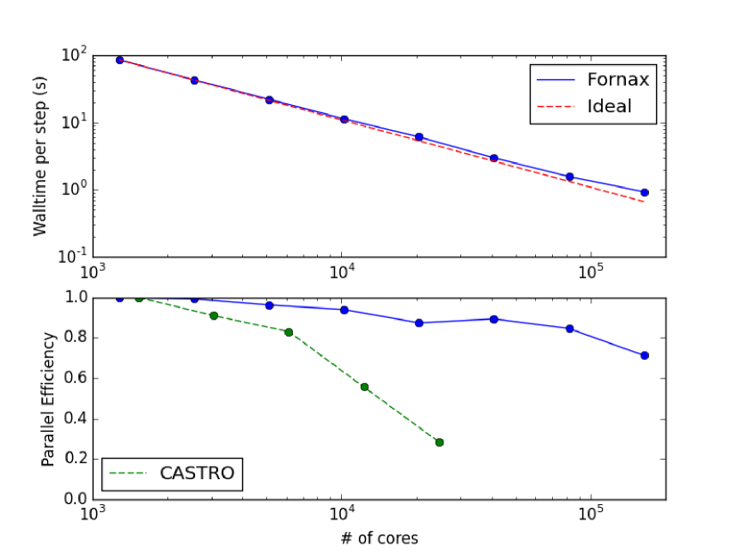
The various radiation species (photons or neutrinos) are followed using an explicit Godunov method applied to the radiation transport operators, but an implicit method is used for the radiation source terms. In this way, the radiative transport is handled locally, without the need for a global solution on the entire mesh. This is also the recent approach taken by Just, Obergaulinger, & Janka (2015), Roberts et al. (2016), and O’Connor & Couch (2018), though with some important differences. By addressing the transport operator with an explicit method, we significantly reduce the computational complexity and communication overhead of traditional multi-dimensional radiative transfer schemes by circumventing the need for global iterative solvers that have typically shown to be slow and/or problematic beyond similar-to\sim10,000 cores. We have demonstrated excellent strong scaling in three dimensions well beyond 100,000 MPI tasks using Fornax on KNL and Cray architectures (Appendix §E).

The light-crossing time of a zone generally sets the time step, but since the speed of light and the speed of sound in the inner core are not far apart in the core-collapse problem after bounce, this numerical stability constraint on the time step is similar to the CFL constraint of the explicit hydrodynamics. For cases in which this near correspondence does not obtain, we have implemented a reduced-speed-of-light approximation, although we do not employ this approximation in our core-collapse simulations. Radiation quantities are reconstructed with linear profiles and an HLLE-like solver is used to determine numerical fluxes at zone boundaries. These HLLE fluxes are corrected to obtain the correct asymptotic behavior in the diffusion limit (Berthon, Charrier, & Dubroca, 2007). The momentum and energy transfer between the radiation and the gas are operator-split and addressed implicitly.

When using spherical coordinates in 2-d and 3-d, gravity is handled with a multipole solver (Müller & Steinmetz 1995), where we generally set the maximum spherical harmonic order necessary equal to twelve. The monopole gravitational term is altered to approximate general-relativistic (GR) gravity (Marek et al. 2006), and we employ the metric terms, grrsubscript𝑔𝑟𝑟g_{rr} and gttsubscript𝑔𝑡𝑡g_{tt}, derived from this potential in the neutrino transport equations to incorporate general relativistic redshift effects (in the manner of Rampp & Janka 2002; see also Skinner et al. 2016). For the CCSN problem, we have used for our recent 2-d and 3-d simulations the K=220 MeV𝐾220 MeVK=220\text{ MeV} equation of state (EOS) of Lattimer & Swesty (1991), the SFHo EOS (Steiner et al. 2013), and the DD2 EOS (Typel et al. 2010; Hempel & Schaffner-Bielich 2010).

With gravity, energy conservation is excellent before and after core bounce (§8.9). However, as with all other supernova codes, at bounce the total energy as defined in integral form experiences a glitch by 1049absentsuperscript1049\geq 10^{49} erg,111In comparison, most supernova codes experience a jump in the total energy at bounce in excess of 1050 erg. due to the fact that the gravitational terms are traditionally handled in the momentum and energy equations as source terms, hence the equations are not solved in conservation form.

Though constructed originally for the CCSN problem, Fornax is a flexible general radiation-hydrodynamics code that functions well in a variety of geometries and coordinate systems. As already stated, in this paper we focus on this generic character as we demonstrate its strengths and capabilities and do not here emphasize its implementation in its original CCSN context. This we leave to a future paper geared specifically to the use of Fornax in studying CCSNe. Again, the main advantages of the Fornax code are its efficiency due to its use of explicit transport, its excellent strong scaling to hundreds of thousands of cores (Appendix §E), its multi-dimensional transport capabilities, and its interior static mesh derefinement near spherical coordinate singularities (§7).

3. Formulation of the Equations

In Fornax, we use a general covariant formalism based on an arbitrary orthogonal metric to write our equations in a way that makes no reference to any particular geometry or set of coordinates. Perhaps the biggest advantage of this approach is flexibility; as we discuss below, switching geometries and coordinates in Fornax is straightforward.

3.1. Hydrodynamics

As is standard practice, we denote contravariant components of a vector with raised indices, covariant components with lowered indices, covariant differentiation with a semicolon, partial differentiation with a comma, and make use of Einstein notation for summation over repeated indices. Here and throughout this work, we adopt a coordinate basis. In this notation, the equations of Newtonian hydrodynamics can be written

ρ,t+(ρvi);i\displaystyle\rho_{,t}+(\rho v^{i})_{;i} =0,absent0\displaystyle=0\,, (1a)
(ρvj),t+(ρvivj+Pδji);i\displaystyle(\rho v_{j})_{,t}+(\rho v^{i}v_{j}+P\mathchoice{\delta^{\leavevmode{i}\mathchoice{\makebox[3.28334pt][c]{$\displaystyle$}}{\makebox[3.28334pt][c]{$\textstyle$}}{\makebox[2.29834pt][c]{$\scriptstyle$}}{\makebox[1.64166pt][c]{$\scriptscriptstyle$}}}_{\mathchoice{\makebox[2.41159pt][c]{$\displaystyle$}}{\makebox[2.41159pt][c]{$\textstyle$}}{\makebox[1.68811pt][c]{$\scriptstyle$}}{\makebox[1.2058pt][c]{$\scriptscriptstyle$}}\leavevmode{j}}}{\delta^{\leavevmode{i}\mathchoice{\makebox[3.28334pt][c]{$\displaystyle$}}{\makebox[3.28334pt][c]{$\textstyle$}}{\makebox[2.29834pt][c]{$\scriptstyle$}}{\makebox[1.64166pt][c]{$\scriptscriptstyle$}}}_{\mathchoice{\makebox[2.41159pt][c]{$\displaystyle$}}{\makebox[2.41159pt][c]{$\textstyle$}}{\makebox[1.68811pt][c]{$\scriptstyle$}}{\makebox[1.2058pt][c]{$\scriptscriptstyle$}}\leavevmode{j}}}{\delta^{\leavevmode{i}\mathchoice{\makebox[3.28334pt][c]{$\displaystyle$}}{\makebox[3.28334pt][c]{$\textstyle$}}{\makebox[2.29834pt][c]{$\scriptstyle$}}{\makebox[1.64166pt][c]{$\scriptscriptstyle$}}}_{\mathchoice{\makebox[2.41159pt][c]{$\displaystyle$}}{\makebox[2.41159pt][c]{$\textstyle$}}{\makebox[1.68811pt][c]{$\scriptstyle$}}{\makebox[1.2058pt][c]{$\scriptscriptstyle$}}\leavevmode{j}}}{\delta^{\leavevmode{i}\mathchoice{\makebox[3.28334pt][c]{$\displaystyle$}}{\makebox[3.28334pt][c]{$\textstyle$}}{\makebox[2.29834pt][c]{$\scriptstyle$}}{\makebox[1.64166pt][c]{$\scriptscriptstyle$}}}_{\mathchoice{\makebox[2.41159pt][c]{$\displaystyle$}}{\makebox[2.41159pt][c]{$\textstyle$}}{\makebox[1.68811pt][c]{$\scriptstyle$}}{\makebox[1.2058pt][c]{$\scriptscriptstyle$}}\leavevmode{j}}})_{;i} =Sj,absentsubscript𝑆𝑗\displaystyle=S_{j}\,, (1b)
(ρe),t+[ρvi(e+Pρ)];i\displaystyle\left(\rho e\right)_{,t}+\left[\rho v^{i}\left(e+\frac{P}{\rho}\right)\right]_{;i} =SE,absentsubscript𝑆𝐸\displaystyle=S_{E}\,, (1c)
(ρX),t+(ρXvi);i\displaystyle(\rho X)_{,t}+(\rho Xv^{i})_{;i} =SX,absentsubscript𝑆𝑋\displaystyle=S_{X}\,, (1d)

where e𝑒e is the specific total energy of the gas, X𝑋X is an arbitrary scalar quantity that may represent, e.g., composition, and Sjsubscript𝑆𝑗S_{j}, SEsubscript𝑆𝐸S_{E}, and SXsubscript𝑆𝑋S_{X} are source terms that account for additional physics. The contravariant components of the velocity are vi=dxi/dtsuperscript𝑣𝑖𝑑superscript𝑥𝑖𝑑𝑡v^{i}=dx^{i}/dt, i.e., they are coordinate velocities. In a coordinate basis, the covariant derivatives can be expanded to yield

ρ,t+1g(gρvi),i\displaystyle\rho_{,t}+\frac{1}{\sqrt{g}}(\sqrt{g}\,\rho v^{i})_{,i} =0,absent0\displaystyle=0\,, (2a)
(ρvj),t+1g[gTji],i\displaystyle(\rho v_{j})_{,t}+\frac{1}{\sqrt{g}}\left[\sqrt{g}\,\mathchoice{T^{\leavevmode{i}\mathchoice{\makebox[3.28334pt][c]{$\displaystyle$}}{\makebox[3.28334pt][c]{$\textstyle$}}{\makebox[2.29834pt][c]{$\scriptstyle$}}{\makebox[1.64166pt][c]{$\scriptscriptstyle$}}}_{\mathchoice{\makebox[2.41159pt][c]{$\displaystyle$}}{\makebox[2.41159pt][c]{$\textstyle$}}{\makebox[1.68811pt][c]{$\scriptstyle$}}{\makebox[1.2058pt][c]{$\scriptscriptstyle$}}\leavevmode{j}}}{T^{\leavevmode{i}\mathchoice{\makebox[3.28334pt][c]{$\displaystyle$}}{\makebox[3.28334pt][c]{$\textstyle$}}{\makebox[2.29834pt][c]{$\scriptstyle$}}{\makebox[1.64166pt][c]{$\scriptscriptstyle$}}}_{\mathchoice{\makebox[2.41159pt][c]{$\displaystyle$}}{\makebox[2.41159pt][c]{$\textstyle$}}{\makebox[1.68811pt][c]{$\scriptstyle$}}{\makebox[1.2058pt][c]{$\scriptscriptstyle$}}\leavevmode{j}}}{T^{\leavevmode{i}\mathchoice{\makebox[3.28334pt][c]{$\displaystyle$}}{\makebox[3.28334pt][c]{$\textstyle$}}{\makebox[2.29834pt][c]{$\scriptstyle$}}{\makebox[1.64166pt][c]{$\scriptscriptstyle$}}}_{\mathchoice{\makebox[2.41159pt][c]{$\displaystyle$}}{\makebox[2.41159pt][c]{$\textstyle$}}{\makebox[1.68811pt][c]{$\scriptstyle$}}{\makebox[1.2058pt][c]{$\scriptscriptstyle$}}\leavevmode{j}}}{T^{\leavevmode{i}\mathchoice{\makebox[3.28334pt][c]{$\displaystyle$}}{\makebox[3.28334pt][c]{$\textstyle$}}{\makebox[2.29834pt][c]{$\scriptstyle$}}{\makebox[1.64166pt][c]{$\scriptscriptstyle$}}}_{\mathchoice{\makebox[2.41159pt][c]{$\displaystyle$}}{\makebox[2.41159pt][c]{$\textstyle$}}{\makebox[1.68811pt][c]{$\scriptstyle$}}{\makebox[1.2058pt][c]{$\scriptscriptstyle$}}\leavevmode{j}}}\right]_{,i} =ΓjklTlk+Sj,absentsubscriptsuperscriptΓ𝑙𝑗𝑘subscriptsuperscript𝑇𝑘𝑙subscript𝑆𝑗\displaystyle=\Gamma^{l}_{jk}\mathchoice{T^{\leavevmode{k}\mathchoice{\makebox[2.2264pt][c]{$\displaystyle$}}{\makebox[2.2264pt][c]{$\textstyle$}}{\makebox[1.55847pt][c]{$\scriptstyle$}}{\makebox[1.11319pt][c]{$\scriptscriptstyle$}}}_{\mathchoice{\makebox[3.86458pt][c]{$\displaystyle$}}{\makebox[3.86458pt][c]{$\textstyle$}}{\makebox[2.7052pt][c]{$\scriptstyle$}}{\makebox[1.93228pt][c]{$\scriptscriptstyle$}}\leavevmode{l}}}{T^{\leavevmode{k}\mathchoice{\makebox[2.2264pt][c]{$\displaystyle$}}{\makebox[2.2264pt][c]{$\textstyle$}}{\makebox[1.55847pt][c]{$\scriptstyle$}}{\makebox[1.11319pt][c]{$\scriptscriptstyle$}}}_{\mathchoice{\makebox[3.86458pt][c]{$\displaystyle$}}{\makebox[3.86458pt][c]{$\textstyle$}}{\makebox[2.7052pt][c]{$\scriptstyle$}}{\makebox[1.93228pt][c]{$\scriptscriptstyle$}}\leavevmode{l}}}{T^{\leavevmode{k}\mathchoice{\makebox[2.2264pt][c]{$\displaystyle$}}{\makebox[2.2264pt][c]{$\textstyle$}}{\makebox[1.55847pt][c]{$\scriptstyle$}}{\makebox[1.11319pt][c]{$\scriptscriptstyle$}}}_{\mathchoice{\makebox[3.86458pt][c]{$\displaystyle$}}{\makebox[3.86458pt][c]{$\textstyle$}}{\makebox[2.7052pt][c]{$\scriptstyle$}}{\makebox[1.93228pt][c]{$\scriptscriptstyle$}}\leavevmode{l}}}{T^{\leavevmode{k}\mathchoice{\makebox[2.2264pt][c]{$\displaystyle$}}{\makebox[2.2264pt][c]{$\textstyle$}}{\makebox[1.55847pt][c]{$\scriptstyle$}}{\makebox[1.11319pt][c]{$\scriptscriptstyle$}}}_{\mathchoice{\makebox[3.86458pt][c]{$\displaystyle$}}{\makebox[3.86458pt][c]{$\textstyle$}}{\makebox[2.7052pt][c]{$\scriptstyle$}}{\makebox[1.93228pt][c]{$\scriptscriptstyle$}}\leavevmode{l}}}+S_{j}\,, (2b)
(ρe),t+1g[gρvi(e+Pρ)],i\displaystyle\left(\rho e\right)_{,t}+\frac{1}{\sqrt{g}}\,\left[\sqrt{g}\rho v^{i}\left(e+\frac{P}{\rho}\right)\right]_{,i} =SE,absentsubscript𝑆𝐸\displaystyle=S_{E}\,, (2c)
(ρX),t+1g(gρXvi),i\displaystyle(\rho X)_{,t}+\frac{1}{\sqrt{g}}\Big{(}\sqrt{g}\,\rho Xv^{i}\Big{)}_{,i} =SX,absentsubscript𝑆𝑋\displaystyle=S_{X}\,, (2d)

where g𝑔g is the determinant of the metric, ΓjklsubscriptsuperscriptΓ𝑙𝑗𝑘\Gamma^{l}_{\;jk} are the Christoffel symbols, defined in terms of derivatives of the metric, and Tlkρvivj+Pδjisubscriptsuperscript𝑇𝑘𝑙𝜌superscript𝑣𝑖subscript𝑣𝑗𝑃subscriptsuperscript𝛿𝑖𝑗\mathchoice{T^{\leavevmode{k}\mathchoice{\makebox[2.2264pt][c]{$\displaystyle$}}{\makebox[2.2264pt][c]{$\textstyle$}}{\makebox[1.55847pt][c]{$\scriptstyle$}}{\makebox[1.11319pt][c]{$\scriptscriptstyle$}}}_{\mathchoice{\makebox[3.86458pt][c]{$\displaystyle$}}{\makebox[3.86458pt][c]{$\textstyle$}}{\makebox[2.7052pt][c]{$\scriptstyle$}}{\makebox[1.93228pt][c]{$\scriptscriptstyle$}}\leavevmode{l}}}{T^{\leavevmode{k}\mathchoice{\makebox[2.2264pt][c]{$\displaystyle$}}{\makebox[2.2264pt][c]{$\textstyle$}}{\makebox[1.55847pt][c]{$\scriptstyle$}}{\makebox[1.11319pt][c]{$\scriptscriptstyle$}}}_{\mathchoice{\makebox[3.86458pt][c]{$\displaystyle$}}{\makebox[3.86458pt][c]{$\textstyle$}}{\makebox[2.7052pt][c]{$\scriptstyle$}}{\makebox[1.93228pt][c]{$\scriptscriptstyle$}}\leavevmode{l}}}{T^{\leavevmode{k}\mathchoice{\makebox[2.2264pt][c]{$\displaystyle$}}{\makebox[2.2264pt][c]{$\textstyle$}}{\makebox[1.55847pt][c]{$\scriptstyle$}}{\makebox[1.11319pt][c]{$\scriptscriptstyle$}}}_{\mathchoice{\makebox[3.86458pt][c]{$\displaystyle$}}{\makebox[3.86458pt][c]{$\textstyle$}}{\makebox[2.7052pt][c]{$\scriptstyle$}}{\makebox[1.93228pt][c]{$\scriptscriptstyle$}}\leavevmode{l}}}{T^{\leavevmode{k}\mathchoice{\makebox[2.2264pt][c]{$\displaystyle$}}{\makebox[2.2264pt][c]{$\textstyle$}}{\makebox[1.55847pt][c]{$\scriptstyle$}}{\makebox[1.11319pt][c]{$\scriptscriptstyle$}}}_{\mathchoice{\makebox[3.86458pt][c]{$\displaystyle$}}{\makebox[3.86458pt][c]{$\textstyle$}}{\makebox[2.7052pt][c]{$\scriptstyle$}}{\makebox[1.93228pt][c]{$\scriptscriptstyle$}}\leavevmode{l}}}\equiv\rho v^{i}v_{j}+P\mathchoice{\delta^{\leavevmode{i}\mathchoice{\makebox[3.28334pt][c]{$\displaystyle$}}{\makebox[3.28334pt][c]{$\textstyle$}}{\makebox[2.29834pt][c]{$\scriptstyle$}}{\makebox[1.64166pt][c]{$\scriptscriptstyle$}}}_{\mathchoice{\makebox[2.41159pt][c]{$\displaystyle$}}{\makebox[2.41159pt][c]{$\textstyle$}}{\makebox[1.68811pt][c]{$\scriptstyle$}}{\makebox[1.2058pt][c]{$\scriptscriptstyle$}}\leavevmode{j}}}{\delta^{\leavevmode{i}\mathchoice{\makebox[3.28334pt][c]{$\displaystyle$}}{\makebox[3.28334pt][c]{$\textstyle$}}{\makebox[2.29834pt][c]{$\scriptstyle$}}{\makebox[1.64166pt][c]{$\scriptscriptstyle$}}}_{\mathchoice{\makebox[2.41159pt][c]{$\displaystyle$}}{\makebox[2.41159pt][c]{$\textstyle$}}{\makebox[1.68811pt][c]{$\scriptstyle$}}{\makebox[1.2058pt][c]{$\scriptscriptstyle$}}\leavevmode{j}}}{\delta^{\leavevmode{i}\mathchoice{\makebox[3.28334pt][c]{$\displaystyle$}}{\makebox[3.28334pt][c]{$\textstyle$}}{\makebox[2.29834pt][c]{$\scriptstyle$}}{\makebox[1.64166pt][c]{$\scriptscriptstyle$}}}_{\mathchoice{\makebox[2.41159pt][c]{$\displaystyle$}}{\makebox[2.41159pt][c]{$\textstyle$}}{\makebox[1.68811pt][c]{$\scriptstyle$}}{\makebox[1.2058pt][c]{$\scriptscriptstyle$}}\leavevmode{j}}}{\delta^{\leavevmode{i}\mathchoice{\makebox[3.28334pt][c]{$\displaystyle$}}{\makebox[3.28334pt][c]{$\textstyle$}}{\makebox[2.29834pt][c]{$\scriptstyle$}}{\makebox[1.64166pt][c]{$\scriptscriptstyle$}}}_{\mathchoice{\makebox[2.41159pt][c]{$\displaystyle$}}{\makebox[2.41159pt][c]{$\textstyle$}}{\makebox[1.68811pt][c]{$\scriptstyle$}}{\makebox[1.2058pt][c]{$\scriptscriptstyle$}}\leavevmode{j}}} is the fluid stress tensor.

Note that we have chosen to express the momentum equation as a conservation law for the covariant compenents of the momentum. There is good reason to do so. Written this way, the geometric source terms, ΓjklTlksubscriptsuperscriptΓ𝑙𝑗𝑘subscriptsuperscript𝑇𝑘𝑙\Gamma^{l}_{jk}\mathchoice{T^{\leavevmode{k}\mathchoice{\makebox[2.2264pt][c]{$\displaystyle$}}{\makebox[2.2264pt][c]{$\textstyle$}}{\makebox[1.55847pt][c]{$\scriptstyle$}}{\makebox[1.11319pt][c]{$\scriptscriptstyle$}}}_{\mathchoice{\makebox[3.86458pt][c]{$\displaystyle$}}{\makebox[3.86458pt][c]{$\textstyle$}}{\makebox[2.7052pt][c]{$\scriptstyle$}}{\makebox[1.93228pt][c]{$\scriptscriptstyle$}}\leavevmode{l}}}{T^{\leavevmode{k}\mathchoice{\makebox[2.2264pt][c]{$\displaystyle$}}{\makebox[2.2264pt][c]{$\textstyle$}}{\makebox[1.55847pt][c]{$\scriptstyle$}}{\makebox[1.11319pt][c]{$\scriptscriptstyle$}}}_{\mathchoice{\makebox[3.86458pt][c]{$\displaystyle$}}{\makebox[3.86458pt][c]{$\textstyle$}}{\makebox[2.7052pt][c]{$\scriptstyle$}}{\makebox[1.93228pt][c]{$\scriptscriptstyle$}}\leavevmode{l}}}{T^{\leavevmode{k}\mathchoice{\makebox[2.2264pt][c]{$\displaystyle$}}{\makebox[2.2264pt][c]{$\textstyle$}}{\makebox[1.55847pt][c]{$\scriptstyle$}}{\makebox[1.11319pt][c]{$\scriptscriptstyle$}}}_{\mathchoice{\makebox[3.86458pt][c]{$\displaystyle$}}{\makebox[3.86458pt][c]{$\textstyle$}}{\makebox[2.7052pt][c]{$\scriptstyle$}}{\makebox[1.93228pt][c]{$\scriptscriptstyle$}}\leavevmode{l}}}{T^{\leavevmode{k}\mathchoice{\makebox[2.2264pt][c]{$\displaystyle$}}{\makebox[2.2264pt][c]{$\textstyle$}}{\makebox[1.55847pt][c]{$\scriptstyle$}}{\makebox[1.11319pt][c]{$\scriptscriptstyle$}}}_{\mathchoice{\makebox[3.86458pt][c]{$\displaystyle$}}{\makebox[3.86458pt][c]{$\textstyle$}}{\makebox[2.7052pt][c]{$\scriptstyle$}}{\makebox[1.93228pt][c]{$\scriptscriptstyle$}}\leavevmode{l}}}, vanish identically for components associated with ignorable coordinates in the metric. A good example is in spherical (r𝑟r, θ𝜃\theta, ϕitalic-ϕ\phi) coordinates where, since ϕitalic-ϕ\phi does not explicitly enter into the metric, the geometric source terms vanish for the ρvϕ𝜌subscript𝑣italic-ϕ\rho v_{\phi} equation. Physically, ρvϕ𝜌subscript𝑣italic-ϕ\rho v_{\phi} is the angular momentum, so we are left with an explicit expression of angular momentum conservation that the numerics will satisfy to machine precision, rather than to the level of truncation error. In general, the covariant expression of the momentum equation respects the geometry of the problem without special consideration or coordinate-specific modifications of the code.

3.2. Radiation

Fornax evolves the zeroth and first moments of the frequency-dependent comoving-frame radiation transport equation. Keeping all terms to 𝒪(v/c)𝒪𝑣𝑐\mathcal{O}(v/c) and dropping terms proportional to the fluid acceleration, the monochromatic radiation moment equations can be written

Eν,t+(Fνi+viEν);i\displaystyle E_{\nu,t}+(F_{\nu}^{i}+v^{i}E_{\nu})_{;i}\qquad
+v;ji[Pνijν(νPνij)]subscriptsuperscript𝑣𝑖𝑗delimited-[]superscriptsubscript𝑃𝜈𝑖𝑗subscript𝜈𝜈superscriptsubscript𝑃𝜈𝑖𝑗\displaystyle+\,\mathchoice{v^{\leavevmode{i}\mathchoice{\makebox[6.39444pt][c]{$\displaystyle$}}{\makebox[6.39444pt][c]{$\textstyle$}}{\makebox[3.65945pt][c]{$\scriptstyle$}}{\makebox[2.61388pt][c]{$\scriptscriptstyle$}}}_{\mathchoice{\makebox[2.41159pt][c]{$\displaystyle$}}{\makebox[2.41159pt][c]{$\textstyle$}}{\makebox[1.68811pt][c]{$\scriptstyle$}}{\makebox[1.2058pt][c]{$\scriptscriptstyle$}}\leavevmode{;j}}}{v^{\leavevmode{i}\mathchoice{\makebox[6.39444pt][c]{$\displaystyle$}}{\makebox[6.39444pt][c]{$\textstyle$}}{\makebox[3.65945pt][c]{$\scriptstyle$}}{\makebox[2.61388pt][c]{$\scriptscriptstyle$}}}_{\mathchoice{\makebox[2.41159pt][c]{$\displaystyle$}}{\makebox[2.41159pt][c]{$\textstyle$}}{\makebox[1.68811pt][c]{$\scriptstyle$}}{\makebox[1.2058pt][c]{$\scriptscriptstyle$}}\leavevmode{;j}}}{v^{\leavevmode{i}\mathchoice{\makebox[6.39444pt][c]{$\displaystyle$}}{\makebox[6.39444pt][c]{$\textstyle$}}{\makebox[3.65945pt][c]{$\scriptstyle$}}{\makebox[2.61388pt][c]{$\scriptscriptstyle$}}}_{\mathchoice{\makebox[2.41159pt][c]{$\displaystyle$}}{\makebox[2.41159pt][c]{$\textstyle$}}{\makebox[1.68811pt][c]{$\scriptstyle$}}{\makebox[1.2058pt][c]{$\scriptscriptstyle$}}\leavevmode{;j}}}{v^{\leavevmode{i}\mathchoice{\makebox[6.39444pt][c]{$\displaystyle$}}{\makebox[6.39444pt][c]{$\textstyle$}}{\makebox[3.65945pt][c]{$\scriptstyle$}}{\makebox[2.61388pt][c]{$\scriptscriptstyle$}}}_{\mathchoice{\makebox[2.41159pt][c]{$\displaystyle$}}{\makebox[2.41159pt][c]{$\textstyle$}}{\makebox[1.68811pt][c]{$\scriptstyle$}}{\makebox[1.2058pt][c]{$\scriptscriptstyle$}}\leavevmode{;j}}}\left[P_{\nu i}^{j}-\partial_{\nu}\left(\nu P_{\nu i}^{j}\right)\right] =RνE,absentsubscript𝑅𝜈𝐸\displaystyle=R_{\nu E}\,, (3a)
Fνj,t+(c2Pνji+viFνj);i\displaystyle F_{\nu j,t}+(c^{2}P_{\nu j}^{i}+v^{i}F_{\nu j})_{;i}\qquad
+v;jiFνiv;kiν(νQνjik)subscriptsuperscript𝑣𝑖𝑗subscript𝐹𝜈𝑖subscriptsuperscript𝑣𝑖𝑘subscript𝜈𝜈subscriptsuperscript𝑄𝑘𝜈𝑗𝑖\displaystyle+\,\mathchoice{v^{\leavevmode{i}\mathchoice{\makebox[6.39444pt][c]{$\displaystyle$}}{\makebox[6.39444pt][c]{$\textstyle$}}{\makebox[3.65945pt][c]{$\scriptstyle$}}{\makebox[2.61388pt][c]{$\scriptscriptstyle$}}}_{\mathchoice{\makebox[2.41159pt][c]{$\displaystyle$}}{\makebox[2.41159pt][c]{$\textstyle$}}{\makebox[1.68811pt][c]{$\scriptstyle$}}{\makebox[1.2058pt][c]{$\scriptscriptstyle$}}\leavevmode{;j}}}{v^{\leavevmode{i}\mathchoice{\makebox[6.39444pt][c]{$\displaystyle$}}{\makebox[6.39444pt][c]{$\textstyle$}}{\makebox[3.65945pt][c]{$\scriptstyle$}}{\makebox[2.61388pt][c]{$\scriptscriptstyle$}}}_{\mathchoice{\makebox[2.41159pt][c]{$\displaystyle$}}{\makebox[2.41159pt][c]{$\textstyle$}}{\makebox[1.68811pt][c]{$\scriptstyle$}}{\makebox[1.2058pt][c]{$\scriptscriptstyle$}}\leavevmode{;j}}}{v^{\leavevmode{i}\mathchoice{\makebox[6.39444pt][c]{$\displaystyle$}}{\makebox[6.39444pt][c]{$\textstyle$}}{\makebox[3.65945pt][c]{$\scriptstyle$}}{\makebox[2.61388pt][c]{$\scriptscriptstyle$}}}_{\mathchoice{\makebox[2.41159pt][c]{$\displaystyle$}}{\makebox[2.41159pt][c]{$\textstyle$}}{\makebox[1.68811pt][c]{$\scriptstyle$}}{\makebox[1.2058pt][c]{$\scriptscriptstyle$}}\leavevmode{;j}}}{v^{\leavevmode{i}\mathchoice{\makebox[6.39444pt][c]{$\displaystyle$}}{\makebox[6.39444pt][c]{$\textstyle$}}{\makebox[3.65945pt][c]{$\scriptstyle$}}{\makebox[2.61388pt][c]{$\scriptscriptstyle$}}}_{\mathchoice{\makebox[2.41159pt][c]{$\displaystyle$}}{\makebox[2.41159pt][c]{$\textstyle$}}{\makebox[1.68811pt][c]{$\scriptstyle$}}{\makebox[1.2058pt][c]{$\scriptscriptstyle$}}\leavevmode{;j}}}F_{\nu i}-\mathchoice{v^{\leavevmode{i}\mathchoice{\makebox[6.97568pt][c]{$\displaystyle$}}{\makebox[6.97568pt][c]{$\textstyle$}}{\makebox[4.06631pt][c]{$\scriptstyle$}}{\makebox[2.9045pt][c]{$\scriptscriptstyle$}}}_{\mathchoice{\makebox[2.41159pt][c]{$\displaystyle$}}{\makebox[2.41159pt][c]{$\textstyle$}}{\makebox[1.68811pt][c]{$\scriptstyle$}}{\makebox[1.2058pt][c]{$\scriptscriptstyle$}}\leavevmode{;k}}}{v^{\leavevmode{i}\mathchoice{\makebox[6.97568pt][c]{$\displaystyle$}}{\makebox[6.97568pt][c]{$\textstyle$}}{\makebox[4.06631pt][c]{$\scriptstyle$}}{\makebox[2.9045pt][c]{$\scriptscriptstyle$}}}_{\mathchoice{\makebox[2.41159pt][c]{$\displaystyle$}}{\makebox[2.41159pt][c]{$\textstyle$}}{\makebox[1.68811pt][c]{$\scriptstyle$}}{\makebox[1.2058pt][c]{$\scriptscriptstyle$}}\leavevmode{;k}}}{v^{\leavevmode{i}\mathchoice{\makebox[6.97568pt][c]{$\displaystyle$}}{\makebox[6.97568pt][c]{$\textstyle$}}{\makebox[4.06631pt][c]{$\scriptstyle$}}{\makebox[2.9045pt][c]{$\scriptscriptstyle$}}}_{\mathchoice{\makebox[2.41159pt][c]{$\displaystyle$}}{\makebox[2.41159pt][c]{$\textstyle$}}{\makebox[1.68811pt][c]{$\scriptstyle$}}{\makebox[1.2058pt][c]{$\scriptscriptstyle$}}\leavevmode{;k}}}{v^{\leavevmode{i}\mathchoice{\makebox[6.97568pt][c]{$\displaystyle$}}{\makebox[6.97568pt][c]{$\textstyle$}}{\makebox[4.06631pt][c]{$\scriptstyle$}}{\makebox[2.9045pt][c]{$\scriptscriptstyle$}}}_{\mathchoice{\makebox[2.41159pt][c]{$\displaystyle$}}{\makebox[2.41159pt][c]{$\textstyle$}}{\makebox[1.68811pt][c]{$\scriptstyle$}}{\makebox[1.2058pt][c]{$\scriptscriptstyle$}}\leavevmode{;k}}}\,\partial_{\nu}\left(\nu Q^{k}_{\nu ji}\right) =Rνj.absentsubscript𝑅𝜈𝑗\displaystyle=R_{\nu j}\,. (3b)

In equations (3), Eνsubscript𝐸𝜈E_{\nu} and Fνjsubscript𝐹𝜈𝑗F_{\nu j} denote the monochromatic energy density and flux of the radiation field at frequency ν𝜈\nu in the comoving frame, Pνijsubscriptsuperscript𝑃𝑗𝜈𝑖P^{j}_{\nu i} is the radiation pressure tensor (2ndsuperscript2nd2^{\rm nd} moment), Qνjiksubscriptsuperscript𝑄𝑘𝜈𝑗𝑖Q^{k}_{\nu ji} is the heat-flux tensor (3rdsuperscript3rd3^{\rm rd} moment), and RνEsubscript𝑅𝜈𝐸R_{\nu E} and Rνjsubscript𝑅𝜈𝑗R_{\nu j} are source terms that account for interactions between the radiation and matter. These interaction terms are written

RνEsubscript𝑅𝜈𝐸\displaystyle R_{\nu E} =jνcκνEν,absentsubscript𝑗𝜈𝑐subscript𝜅𝜈subscript𝐸𝜈\displaystyle=j_{\nu}-c\kappa_{\nu}E_{\nu}\,, (4a)
Rνjsubscript𝑅𝜈𝑗\displaystyle R_{\nu j} =c(κν+σν)Fνj,absent𝑐subscript𝜅𝜈subscript𝜎𝜈subscript𝐹𝜈𝑗\displaystyle=-c(\kappa_{\nu}+\sigma_{\nu})F_{\nu j}\,, (4b)

where jνsubscript𝑗𝜈j_{\nu} is the emissivity, κνsubscript𝜅𝜈\kappa_{\nu} is the absorption coefficient, and σνsubscript𝜎𝜈\sigma_{\nu} is the scattering coefficient. Correspondingly, there are energy and momentum source terms in the fluid equations:

Sjsubscript𝑆𝑗\displaystyle S_{j} =1c20Rνj𝑑ν,absent1superscript𝑐2superscriptsubscript0subscript𝑅𝜈𝑗differential-d𝜈\displaystyle=-\frac{1}{c^{2}}\int_{0}^{\infty}R_{\nu j}\,d\nu\,, (5a)
SEsubscript𝑆𝐸\displaystyle S_{E} =0(RνE+vic2Rνi)𝑑ν.absentsuperscriptsubscript0subscript𝑅𝜈𝐸superscript𝑣𝑖superscript𝑐2subscript𝑅𝜈𝑖differential-d𝜈\displaystyle=-\int_{0}^{\infty}\left(R_{\nu E}+\frac{v^{i}}{c^{2}}R_{\nu i}\right)d\nu\,. (5b)

As in the fluid sector, we rewrite these covariant derivatives as partial derivatives, introducing geometric source terms in the radiation momentum equation.

Fornax can treat either photon or neutrino radiation fields. For neutrinos, Equations (3) are solved separately for each species, and Equations (5) are summed over species. Additionlly, the electron fraction is evolved according to Equation 2d, with X=Ye𝑋subscript𝑌𝑒X=Y_{e} and

SX=s0ξsν(jsνcκsνEsν)𝑑ν,subscript𝑆𝑋subscript𝑠superscriptsubscript0subscript𝜉𝑠𝜈subscript𝑗𝑠𝜈𝑐subscript𝜅𝑠𝜈subscript𝐸𝑠𝜈differential-d𝜈S_{X}=\sum_{s}\int_{0}^{\infty}\xi_{s\nu}(j_{s\nu}-c\kappa_{s\nu}E_{s\nu})\,d\nu\,, (6)

where s𝑠s refers to the neutrino species and

ξsν={(NAν)1,s=νe(NAν)1,s=ν¯e0,s=νx,subscript𝜉𝑠𝜈casessuperscriptsubscript𝑁𝐴𝜈1𝑠subscript𝜈𝑒superscriptsubscript𝑁𝐴𝜈1𝑠subscript¯𝜈𝑒0𝑠subscript𝜈𝑥\xi_{s\nu}=\begin{cases}-(N_{A}\nu)^{-1},&\text{$s=\nu_{e}$}\\ (N_{A}\nu)^{-1},&\text{$s=\bar{\nu}_{e}$}\\ 0,&\text{$s=\nu_{x}$}\end{cases}\,, (7)

where NAsubscript𝑁𝐴N_{A} is Avogadro’s number.

4. Numerical Discretization

To maintain conservation while admitting discontinuous shock solutions, we adopt a finite-volume discretization of the equations presented in Section 3. Independent of geometry or coordinates (x𝑥x), the volume element can always be expressed dV=gd3x𝑑𝑉𝑔superscript𝑑3𝑥dV=\sqrt{g}\,d^{3}x. Similarly, for arbitrary orthogonal coordinates the area element is dA=gd2x𝑑𝐴𝑔superscript𝑑2𝑥dA=\sqrt{g}\,d^{2}x. Averaging the equations over control volumes (cells) leads to a set of exact equations describing the evolution of cell volume-averaged quantities.

Applying the divergence theorem, we express the divergence terms in each equation as a net flux through cell faces. For example, the volume-averaged density in cell (i,j,k)𝑖𝑗𝑘(i,j,k) evolves according to

dρi,j,kdt=1Vi,j,k×[(ρv0A0)i+1/2,j,k(ρv0A0)i1/2,j,k+(ρv1A1)i,j+1/2,k(ρv1A1)i,j1/2,k+(ρv2A2)i,j,k+1/2(ρv2A2)i,j,k1/2].𝑑subscript𝜌𝑖𝑗𝑘𝑑𝑡1subscript𝑉𝑖𝑗𝑘delimited-[]subscript𝜌superscript𝑣0subscript𝐴0𝑖12𝑗𝑘subscript𝜌superscript𝑣0subscript𝐴0𝑖12𝑗𝑘subscript𝜌superscript𝑣1subscript𝐴1𝑖𝑗12𝑘subscript𝜌superscript𝑣1subscript𝐴1𝑖𝑗12𝑘subscript𝜌superscript𝑣2subscript𝐴2𝑖𝑗𝑘12subscript𝜌superscript𝑣2subscript𝐴2𝑖𝑗𝑘12\begin{split}\frac{d\rho_{i,j,k}}{dt}=-&\frac{1}{V_{i,j,k}}\\ \times[&(\rho v^{0}A_{0})_{i+1/2,j,k}-(\rho v^{0}A_{0})_{i-1/2,j,k}\\ +&(\rho v^{1}A_{1})_{i,j+1/2,k}-(\rho v^{1}A_{1})_{i,j-1/2,k}\\ +&(\rho v^{2}A_{2})_{i,j,k+1/2}-(\rho v^{2}A_{2})_{i,j,k-1/2}]\,.\end{split} (8)

Two things are of note. First, by integrating over cell volumes, we have transformed our set of partial differential equations into a large set of coupled ordinary differential equations. Second, Equation (8) is exact, provided the fluxes on each face are taken to represent cell face area-averaged quantities.

Source terms appear in nearly all the evolution equations and, for consistency, must also be volume-averaged. If these source terms were linear in the conserved variables, this volume averaging would be trivial. Unfortunately, all the source terms are nonlinear, which requires that we make choices for how the volume averaging is carried out. For example, the geometric source terms in Equation 2b are typically treated as

1VgΓjklTlkd3xΓjklTlk(𝐔),1𝑉𝑔subscriptsuperscriptΓ𝑙𝑗𝑘subscriptsuperscript𝑇𝑘𝑙superscript𝑑3𝑥delimited-⟨⟩subscriptsuperscriptΓ𝑙𝑗𝑘subscriptsuperscript𝑇𝑘𝑙delimited-⟨⟩𝐔\frac{1}{V}\int\sqrt{g}\ \Gamma^{l}_{jk}\mathchoice{T^{\leavevmode{k}\mathchoice{\makebox[2.2264pt][c]{$\displaystyle$}}{\makebox[2.2264pt][c]{$\textstyle$}}{\makebox[1.55847pt][c]{$\scriptstyle$}}{\makebox[1.11319pt][c]{$\scriptscriptstyle$}}}_{\mathchoice{\makebox[3.86458pt][c]{$\displaystyle$}}{\makebox[3.86458pt][c]{$\textstyle$}}{\makebox[2.7052pt][c]{$\scriptstyle$}}{\makebox[1.93228pt][c]{$\scriptscriptstyle$}}\leavevmode{l}}}{T^{\leavevmode{k}\mathchoice{\makebox[2.2264pt][c]{$\displaystyle$}}{\makebox[2.2264pt][c]{$\textstyle$}}{\makebox[1.55847pt][c]{$\scriptstyle$}}{\makebox[1.11319pt][c]{$\scriptscriptstyle$}}}_{\mathchoice{\makebox[3.86458pt][c]{$\displaystyle$}}{\makebox[3.86458pt][c]{$\textstyle$}}{\makebox[2.7052pt][c]{$\scriptstyle$}}{\makebox[1.93228pt][c]{$\scriptscriptstyle$}}\leavevmode{l}}}{T^{\leavevmode{k}\mathchoice{\makebox[2.2264pt][c]{$\displaystyle$}}{\makebox[2.2264pt][c]{$\textstyle$}}{\makebox[1.55847pt][c]{$\scriptstyle$}}{\makebox[1.11319pt][c]{$\scriptscriptstyle$}}}_{\mathchoice{\makebox[3.86458pt][c]{$\displaystyle$}}{\makebox[3.86458pt][c]{$\textstyle$}}{\makebox[2.7052pt][c]{$\scriptstyle$}}{\makebox[1.93228pt][c]{$\scriptscriptstyle$}}\leavevmode{l}}}{T^{\leavevmode{k}\mathchoice{\makebox[2.2264pt][c]{$\displaystyle$}}{\makebox[2.2264pt][c]{$\textstyle$}}{\makebox[1.55847pt][c]{$\scriptstyle$}}{\makebox[1.11319pt][c]{$\scriptscriptstyle$}}}_{\mathchoice{\makebox[3.86458pt][c]{$\displaystyle$}}{\makebox[3.86458pt][c]{$\textstyle$}}{\makebox[2.7052pt][c]{$\scriptstyle$}}{\makebox[1.93228pt][c]{$\scriptscriptstyle$}}\leavevmode{l}}}\,d^{3}x\approx\langle\Gamma^{l}_{jk}\rangle\mathchoice{T^{\leavevmode{k}\mathchoice{\makebox[2.2264pt][c]{$\displaystyle$}}{\makebox[2.2264pt][c]{$\textstyle$}}{\makebox[1.55847pt][c]{$\scriptstyle$}}{\makebox[1.11319pt][c]{$\scriptscriptstyle$}}}_{\mathchoice{\makebox[3.86458pt][c]{$\displaystyle$}}{\makebox[3.86458pt][c]{$\textstyle$}}{\makebox[2.7052pt][c]{$\scriptstyle$}}{\makebox[1.93228pt][c]{$\scriptscriptstyle$}}\leavevmode{l}}}{T^{\leavevmode{k}\mathchoice{\makebox[2.2264pt][c]{$\displaystyle$}}{\makebox[2.2264pt][c]{$\textstyle$}}{\makebox[1.55847pt][c]{$\scriptstyle$}}{\makebox[1.11319pt][c]{$\scriptscriptstyle$}}}_{\mathchoice{\makebox[3.86458pt][c]{$\displaystyle$}}{\makebox[3.86458pt][c]{$\textstyle$}}{\makebox[2.7052pt][c]{$\scriptstyle$}}{\makebox[1.93228pt][c]{$\scriptscriptstyle$}}\leavevmode{l}}}{T^{\leavevmode{k}\mathchoice{\makebox[2.2264pt][c]{$\displaystyle$}}{\makebox[2.2264pt][c]{$\textstyle$}}{\makebox[1.55847pt][c]{$\scriptstyle$}}{\makebox[1.11319pt][c]{$\scriptscriptstyle$}}}_{\mathchoice{\makebox[3.86458pt][c]{$\displaystyle$}}{\makebox[3.86458pt][c]{$\textstyle$}}{\makebox[2.7052pt][c]{$\scriptstyle$}}{\makebox[1.93228pt][c]{$\scriptscriptstyle$}}\leavevmode{l}}}{T^{\leavevmode{k}\mathchoice{\makebox[2.2264pt][c]{$\displaystyle$}}{\makebox[2.2264pt][c]{$\textstyle$}}{\makebox[1.55847pt][c]{$\scriptstyle$}}{\makebox[1.11319pt][c]{$\scriptscriptstyle$}}}_{\mathchoice{\makebox[3.86458pt][c]{$\displaystyle$}}{\makebox[3.86458pt][c]{$\textstyle$}}{\makebox[2.7052pt][c]{$\scriptstyle$}}{\makebox[1.93228pt][c]{$\scriptscriptstyle$}}\leavevmode{l}}}(\langle\mathbf{U}\rangle)\,, (9)

where angle brackets indicate a volume average over a given cell and Tlk(𝐔)subscriptsuperscript𝑇𝑘𝑙𝐔\mathchoice{T^{\leavevmode{k}\mathchoice{\makebox[2.2264pt][c]{$\displaystyle$}}{\makebox[2.2264pt][c]{$\textstyle$}}{\makebox[1.55847pt][c]{$\scriptstyle$}}{\makebox[1.11319pt][c]{$\scriptscriptstyle$}}}_{\mathchoice{\makebox[3.86458pt][c]{$\displaystyle$}}{\makebox[3.86458pt][c]{$\textstyle$}}{\makebox[2.7052pt][c]{$\scriptstyle$}}{\makebox[1.93228pt][c]{$\scriptscriptstyle$}}\leavevmode{l}}}{T^{\leavevmode{k}\mathchoice{\makebox[2.2264pt][c]{$\displaystyle$}}{\makebox[2.2264pt][c]{$\textstyle$}}{\makebox[1.55847pt][c]{$\scriptstyle$}}{\makebox[1.11319pt][c]{$\scriptscriptstyle$}}}_{\mathchoice{\makebox[3.86458pt][c]{$\displaystyle$}}{\makebox[3.86458pt][c]{$\textstyle$}}{\makebox[2.7052pt][c]{$\scriptstyle$}}{\makebox[1.93228pt][c]{$\scriptscriptstyle$}}\leavevmode{l}}}{T^{\leavevmode{k}\mathchoice{\makebox[2.2264pt][c]{$\displaystyle$}}{\makebox[2.2264pt][c]{$\textstyle$}}{\makebox[1.55847pt][c]{$\scriptstyle$}}{\makebox[1.11319pt][c]{$\scriptscriptstyle$}}}_{\mathchoice{\makebox[3.86458pt][c]{$\displaystyle$}}{\makebox[3.86458pt][c]{$\textstyle$}}{\makebox[2.7052pt][c]{$\scriptstyle$}}{\makebox[1.93228pt][c]{$\scriptscriptstyle$}}\leavevmode{l}}}{T^{\leavevmode{k}\mathchoice{\makebox[2.2264pt][c]{$\displaystyle$}}{\makebox[2.2264pt][c]{$\textstyle$}}{\makebox[1.55847pt][c]{$\scriptstyle$}}{\makebox[1.11319pt][c]{$\scriptscriptstyle$}}}_{\mathchoice{\makebox[3.86458pt][c]{$\displaystyle$}}{\makebox[3.86458pt][c]{$\textstyle$}}{\makebox[2.7052pt][c]{$\scriptstyle$}}{\makebox[1.93228pt][c]{$\scriptscriptstyle$}}\leavevmode{l}}}(\mathbf{U}) is stress tensor computed from the vector of volume-averaged conserved variables. It is straightforward to show that the error in this approximation is 𝒪(Δx2)𝒪Δsuperscript𝑥2\mathcal{O}(\Delta x^{2}), but this is not a unique second-order accurate expression. Adopting alternative expressions for some geometric source terms can have desirable properties, such as exact conservation of angular momentum (see Appendix §A).

With space fully discretized, we now turn to the issue of temporal evolution. Each of our equations can be written in the form

Qt+(Qi);i=Snonstiff+Sstiff,\frac{\partial Q}{\partial t}+(\mathcal{F}^{i}_{Q})_{;i}=S_{\rm non-stiff}+S_{\rm stiff}\,, (10)

where Q𝑄Q is some volume-averaged quantity evolved on the mesh, Qisubscriptsuperscript𝑖𝑄\mathcal{F}^{i}_{Q} is the area-averaged flux of that quantity, and the volume-averaged source terms have been grouped together according to whether or not they are stiff. The only terms currently treated by Fornax that are stiff are the interaction terms that couple radiation and matter and the terms that handle reactions (nuclear or chemical). These stiff terms require an implicit treatment for numerical stability since the characteristic time scales for these interactions may be extremely short compared to the explicit Courant time step for the matter or radiation. All other terms are treated explicitly and are evolved together without operator splitting. The explicit time integration is currently carried out using Shu & Osher’s (1988) optimal second-order TVD Runge-Kutta scheme.

The frequency dependence of the radiation moments is represented in discrete groups linearly or logarithmically spaced between a user-specified minimum and maximum frequency.222Alternatively, the user may specify the frequency range using equivalent energies in MeV, a standard unit for neutrino radiation. The number of groups per species Nsgsubscript𝑁𝑠𝑔N_{sg} is also set by the user and can be different for each species. Unless otherwise indicated, the radiation moments and interaction coefficients are integrated over each frequency group, appearing with a subscript g𝑔g. For example,

Esgνg1/2νg+1/2Esν𝑑νsubscript𝐸𝑠𝑔superscriptsubscriptsubscript𝜈𝑔12subscript𝜈𝑔12subscript𝐸𝑠𝜈differential-d𝜈E_{sg}\equiv\int_{\nu_{g-1/2}}^{\nu_{g+1/2}}E_{s\nu}\,d\nu (11)

is the energy density of species s𝑠s in group g𝑔g which has units of energy density. In integrating over frequency groups, the monochromatic radiation moment Equations (3) become the group-integrated moment equations, given for each group g𝑔g (and for each species s𝑠s) by

Eg,t+(Fgi+viEg);i\displaystyle E_{g,t}+(F_{g}^{i}+v^{i}E_{g})_{;i}\qquad
+v;ji[Pgijνg1/2νg+1/2ν(νPνij)dν]subscriptsuperscript𝑣𝑖𝑗delimited-[]superscriptsubscript𝑃𝑔𝑖𝑗superscriptsubscriptsubscript𝜈𝑔12subscript𝜈𝑔12subscript𝜈𝜈superscriptsubscript𝑃𝜈𝑖𝑗𝑑𝜈\displaystyle+\,\mathchoice{v^{\leavevmode{i}\mathchoice{\makebox[6.39444pt][c]{$\displaystyle$}}{\makebox[6.39444pt][c]{$\textstyle$}}{\makebox[3.65945pt][c]{$\scriptstyle$}}{\makebox[2.61388pt][c]{$\scriptscriptstyle$}}}_{\mathchoice{\makebox[2.41159pt][c]{$\displaystyle$}}{\makebox[2.41159pt][c]{$\textstyle$}}{\makebox[1.68811pt][c]{$\scriptstyle$}}{\makebox[1.2058pt][c]{$\scriptscriptstyle$}}\leavevmode{;j}}}{v^{\leavevmode{i}\mathchoice{\makebox[6.39444pt][c]{$\displaystyle$}}{\makebox[6.39444pt][c]{$\textstyle$}}{\makebox[3.65945pt][c]{$\scriptstyle$}}{\makebox[2.61388pt][c]{$\scriptscriptstyle$}}}_{\mathchoice{\makebox[2.41159pt][c]{$\displaystyle$}}{\makebox[2.41159pt][c]{$\textstyle$}}{\makebox[1.68811pt][c]{$\scriptstyle$}}{\makebox[1.2058pt][c]{$\scriptscriptstyle$}}\leavevmode{;j}}}{v^{\leavevmode{i}\mathchoice{\makebox[6.39444pt][c]{$\displaystyle$}}{\makebox[6.39444pt][c]{$\textstyle$}}{\makebox[3.65945pt][c]{$\scriptstyle$}}{\makebox[2.61388pt][c]{$\scriptscriptstyle$}}}_{\mathchoice{\makebox[2.41159pt][c]{$\displaystyle$}}{\makebox[2.41159pt][c]{$\textstyle$}}{\makebox[1.68811pt][c]{$\scriptstyle$}}{\makebox[1.2058pt][c]{$\scriptscriptstyle$}}\leavevmode{;j}}}{v^{\leavevmode{i}\mathchoice{\makebox[6.39444pt][c]{$\displaystyle$}}{\makebox[6.39444pt][c]{$\textstyle$}}{\makebox[3.65945pt][c]{$\scriptstyle$}}{\makebox[2.61388pt][c]{$\scriptscriptstyle$}}}_{\mathchoice{\makebox[2.41159pt][c]{$\displaystyle$}}{\makebox[2.41159pt][c]{$\textstyle$}}{\makebox[1.68811pt][c]{$\scriptstyle$}}{\makebox[1.2058pt][c]{$\scriptscriptstyle$}}\leavevmode{;j}}}\left[P_{gi}^{j}-\int_{\nu_{g-1/2}}^{\nu_{g+1/2}}\partial_{\nu}\left(\nu P_{\nu i}^{j}\right)\,d\nu\right] =RgE,absentsubscript𝑅𝑔𝐸\displaystyle=R_{gE}\,, (12a)
Fgj,t+(c2Pgji+viFgj);i\displaystyle F_{gj,t}+(c^{2}P_{gj}^{i}+v^{i}F_{gj})_{;i}\qquad
+v;jiFgiv;kiνg1/2νg+1/2ν(νQνjik)dνsubscriptsuperscript𝑣𝑖𝑗subscript𝐹𝑔𝑖subscriptsuperscript𝑣𝑖𝑘superscriptsubscriptsubscript𝜈𝑔12subscript𝜈𝑔12subscript𝜈𝜈subscriptsuperscript𝑄𝑘𝜈𝑗𝑖𝑑𝜈\displaystyle+\,\mathchoice{v^{\leavevmode{i}\mathchoice{\makebox[6.39444pt][c]{$\displaystyle$}}{\makebox[6.39444pt][c]{$\textstyle$}}{\makebox[3.65945pt][c]{$\scriptstyle$}}{\makebox[2.61388pt][c]{$\scriptscriptstyle$}}}_{\mathchoice{\makebox[2.41159pt][c]{$\displaystyle$}}{\makebox[2.41159pt][c]{$\textstyle$}}{\makebox[1.68811pt][c]{$\scriptstyle$}}{\makebox[1.2058pt][c]{$\scriptscriptstyle$}}\leavevmode{;j}}}{v^{\leavevmode{i}\mathchoice{\makebox[6.39444pt][c]{$\displaystyle$}}{\makebox[6.39444pt][c]{$\textstyle$}}{\makebox[3.65945pt][c]{$\scriptstyle$}}{\makebox[2.61388pt][c]{$\scriptscriptstyle$}}}_{\mathchoice{\makebox[2.41159pt][c]{$\displaystyle$}}{\makebox[2.41159pt][c]{$\textstyle$}}{\makebox[1.68811pt][c]{$\scriptstyle$}}{\makebox[1.2058pt][c]{$\scriptscriptstyle$}}\leavevmode{;j}}}{v^{\leavevmode{i}\mathchoice{\makebox[6.39444pt][c]{$\displaystyle$}}{\makebox[6.39444pt][c]{$\textstyle$}}{\makebox[3.65945pt][c]{$\scriptstyle$}}{\makebox[2.61388pt][c]{$\scriptscriptstyle$}}}_{\mathchoice{\makebox[2.41159pt][c]{$\displaystyle$}}{\makebox[2.41159pt][c]{$\textstyle$}}{\makebox[1.68811pt][c]{$\scriptstyle$}}{\makebox[1.2058pt][c]{$\scriptscriptstyle$}}\leavevmode{;j}}}{v^{\leavevmode{i}\mathchoice{\makebox[6.39444pt][c]{$\displaystyle$}}{\makebox[6.39444pt][c]{$\textstyle$}}{\makebox[3.65945pt][c]{$\scriptstyle$}}{\makebox[2.61388pt][c]{$\scriptscriptstyle$}}}_{\mathchoice{\makebox[2.41159pt][c]{$\displaystyle$}}{\makebox[2.41159pt][c]{$\textstyle$}}{\makebox[1.68811pt][c]{$\scriptstyle$}}{\makebox[1.2058pt][c]{$\scriptscriptstyle$}}\leavevmode{;j}}}F_{gi}-\mathchoice{v^{\leavevmode{i}\mathchoice{\makebox[6.97568pt][c]{$\displaystyle$}}{\makebox[6.97568pt][c]{$\textstyle$}}{\makebox[4.06631pt][c]{$\scriptstyle$}}{\makebox[2.9045pt][c]{$\scriptscriptstyle$}}}_{\mathchoice{\makebox[2.41159pt][c]{$\displaystyle$}}{\makebox[2.41159pt][c]{$\textstyle$}}{\makebox[1.68811pt][c]{$\scriptstyle$}}{\makebox[1.2058pt][c]{$\scriptscriptstyle$}}\leavevmode{;k}}}{v^{\leavevmode{i}\mathchoice{\makebox[6.97568pt][c]{$\displaystyle$}}{\makebox[6.97568pt][c]{$\textstyle$}}{\makebox[4.06631pt][c]{$\scriptstyle$}}{\makebox[2.9045pt][c]{$\scriptscriptstyle$}}}_{\mathchoice{\makebox[2.41159pt][c]{$\displaystyle$}}{\makebox[2.41159pt][c]{$\textstyle$}}{\makebox[1.68811pt][c]{$\scriptstyle$}}{\makebox[1.2058pt][c]{$\scriptscriptstyle$}}\leavevmode{;k}}}{v^{\leavevmode{i}\mathchoice{\makebox[6.97568pt][c]{$\displaystyle$}}{\makebox[6.97568pt][c]{$\textstyle$}}{\makebox[4.06631pt][c]{$\scriptstyle$}}{\makebox[2.9045pt][c]{$\scriptscriptstyle$}}}_{\mathchoice{\makebox[2.41159pt][c]{$\displaystyle$}}{\makebox[2.41159pt][c]{$\textstyle$}}{\makebox[1.68811pt][c]{$\scriptstyle$}}{\makebox[1.2058pt][c]{$\scriptscriptstyle$}}\leavevmode{;k}}}{v^{\leavevmode{i}\mathchoice{\makebox[6.97568pt][c]{$\displaystyle$}}{\makebox[6.97568pt][c]{$\textstyle$}}{\makebox[4.06631pt][c]{$\scriptstyle$}}{\makebox[2.9045pt][c]{$\scriptscriptstyle$}}}_{\mathchoice{\makebox[2.41159pt][c]{$\displaystyle$}}{\makebox[2.41159pt][c]{$\textstyle$}}{\makebox[1.68811pt][c]{$\scriptstyle$}}{\makebox[1.2058pt][c]{$\scriptscriptstyle$}}\leavevmode{;k}}}\int_{\nu_{g-1/2}}^{\nu_{g+1/2}}\partial_{\nu}\left(\nu Q^{k}_{\nu ji}\right)\,d\nu =Rgj.absentsubscript𝑅𝑔𝑗\displaystyle=R_{gj}\,. (12b)

5. Reconstruction, Solvers, and Interaction Terms

5.1. Reconstruction

The hydrodynamics in Fornax is evolved using a directionally-unsplit, high-order Godunov-type scheme. Having already described the underlying spatial discretization of the variables as well as the time-stepping scheme, the essential remaining element is a method for computing fluxes on cell faces. Since Fornax employs Runge-Kutta time stepping, there is no need for the characteristic tracing step or transverse flux gradient corrections required in single-step unsplit schemes. This approach has the great advantage of relative simplicity, especially in the multi-physics context. Fornax follows the standard approach used by similar codes, first reconstructing the state profile at cell faces and then solving the resulting Riemann problem to obtain fluxes.

There are many potential approaches to reconstructing face data based on cell values. One particularly popular approach is to reconstruct the primitive variables (ρ𝜌\rho, P𝑃P, and visuperscript𝑣𝑖v^{i}) using the method described by Woodward & Colella (1984), the so-called piecewise-parabolic method (PPM). This method is based on the idea of reconstructing profiles of the volume-averaged data, with curvilinear coordinates incorporated by reconstructing the profiles in the volume coordinate rather than in the original coordinates themselves. This approach can be problematic in the vicinity of coordinate singularities. Blondin & Lufkin (1993) suggest a generalized approach to PPM in cylindrical and spherical coordinates. Unfortunately, it can be shown that their approach cannot be used generically and, in fact, fails even for standard spherical coordinates. Here, we present an alternative approach that works in arbitrary geometries and coordinates, which contains PPM as a special case.

We begin by writing down an expression for a general nthsuperscript𝑛thn^{\rm th}-order polynomial:

p(x)=j=0ncjxj,𝑝𝑥superscriptsubscript𝑗0𝑛subscript𝑐𝑗superscript𝑥𝑗p(x)=\sum_{j=0}^{n}c_{j}x^{j}\,, (13)

where cjsubscript𝑐𝑗c_{j} is the coefficient of the jthsuperscript𝑗thj^{\rm th}-order monomial. As in PPM, we wish to construct a polynomial p(x)𝑝𝑥p(x) consistent with pisubscript𝑝𝑖p_{i}, the volume average of quantity p𝑝p in cell i𝑖i. In our formulation, the volume average of p(x)𝑝𝑥p(x) must then satisfy a set of constraint equations of the form

pisubscript𝑝𝑖\displaystyle p_{i} =piabsentsubscriptdelimited-⟨⟩𝑝𝑖\displaystyle=\langle p\rangle_{i}
=1Vxi1/2xi+1/2p(x)g𝑑xabsent1𝑉superscriptsubscriptsubscript𝑥𝑖12subscript𝑥𝑖12𝑝𝑥𝑔differential-d𝑥\displaystyle=\frac{1}{V}\int_{x_{i-1/2}}^{x_{i+1/2}}p(x)\sqrt{g}\,dx
=j=0ncjxji,absentsuperscriptsubscript𝑗0𝑛subscript𝑐𝑗subscriptdelimited-⟨⟩superscript𝑥𝑗𝑖\displaystyle=\sum_{j=0}^{n}c_{j}\langle x^{j}\rangle_{i}\,, (14)

where xi±1/2xi±Δx/2subscript𝑥plus-or-minus𝑖12plus-or-minussubscript𝑥𝑖Δ𝑥2x_{i\pm 1/2}\equiv x_{i}\pm\Delta x/2 and the quantities xjisubscriptdelimited-⟨⟩superscript𝑥𝑗𝑖\langle x^{j}\rangle_{i} can be precomputed for each cell either directly or via Romberg integration then stored in one-dimensional arrays. For the case n=0𝑛0n=0, i.e., for piecewise-constant reconstruction, this yields the trivial result that p(x)=pi𝑝𝑥subscript𝑝𝑖p(x)=p_{i}. For n>0𝑛0n>0, we must further constrain the reconstruction. To proceed, we first distinguish between cases where n𝑛n is even and n𝑛n is odd. For odd n𝑛n, we form a symmetric stencil around each edge containing data in n+1𝑛1n+1 cells and require that pi=pisubscriptdelimited-⟨⟩𝑝𝑖subscript𝑝𝑖\langle p\rangle_{i}=p_{i} in each cell i𝑖i. This necessarily yields continuous left and right states at cell interfaces, but that continuity may be broken by the subsequent application of a slope limiter. For even n𝑛n, we similarly constrain the polynomial within a symmetric stencil of n+1𝑛1n+1 cells, this time centered on a given cell, yielding potentially discontinuous data at cell faces even before the application of a slope limiter.

In Fornax, since we most often employ third-order piecewise-parabolic reconstruction (n=2𝑛2n=2), we now describe it in more detail. The reconstruction of p(x)𝑝𝑥p(x) in cell i𝑖i depends on the data values pi1subscript𝑝𝑖1p_{i-1}, pisubscript𝑝𝑖p_{i}, and pi+1subscript𝑝𝑖1p_{i+1}. Note that this requires the same number of ghost cells as linear reconstruction, is of similar cost, and being of higher order, produces superior results for many problems, as we show below and in §8.

To begin, if pisubscript𝑝𝑖p_{i} is a local extremum of the data, then the reconstruction in cell i𝑖i is taken to be piecewise-constant. Otherwise, three constraints in the form of Equation (14) are used to form the linear system

[1xi1x2i11xix2i1xi+1x2i+1][c0c1c2]=[pi1pipi+1],delimited-[]1subscriptdelimited-⟨⟩𝑥𝑖1subscriptdelimited-⟨⟩superscript𝑥2𝑖11subscriptdelimited-⟨⟩𝑥𝑖subscriptdelimited-⟨⟩superscript𝑥2𝑖1subscriptdelimited-⟨⟩𝑥𝑖1subscriptdelimited-⟨⟩superscript𝑥2𝑖1delimited-[]subscript𝑐0subscript𝑐1subscript𝑐2delimited-[]subscript𝑝𝑖1subscript𝑝𝑖subscript𝑝𝑖1\left[\begin{array}[]{lll}1&\langle x\rangle_{i-1}&\langle x^{2}\rangle_{i-1}\\ 1&\langle x\rangle_{i}&\langle x^{2}\rangle_{i}\\ 1&\langle x\rangle_{i+1}&\langle x^{2}\rangle_{i+1}\end{array}\right]\left[\begin{array}[]{l}c_{0}\\ c_{1}\\ c_{2}\end{array}\right]=\left[\begin{array}[]{l}p_{i-1}\\ p_{i}\\ p_{i+1}\end{array}\right], (15)

which is then solved for the unique interpolation coefficients c0subscript𝑐0c_{0}, c1subscript𝑐1c_{1}, and c2subscript𝑐2c_{2}. The resulting polynomial is then used to determine pR,i1/2p(xi1/2)subscript𝑝𝑅𝑖12𝑝subscript𝑥𝑖12p_{R,i-1/2}\equiv p(x_{i-1/2}), the right state at the lower face of cell i𝑖i, and pL,i+1/2p(xi+1/2)subscript𝑝𝐿𝑖12𝑝subscript𝑥𝑖12p_{L,i+1/2}\equiv p(x_{i+1/2}), the left state at the upper face of cell i𝑖i. If pR,i1/2subscript𝑝𝑅𝑖12p_{R,i-1/2} is sufficiently close to either pi1subscript𝑝𝑖1p_{i-1} or pisubscript𝑝𝑖p_{i} such that p(x)𝑝𝑥p(x) has an extremum for x(xi1,xi)𝑥subscript𝑥𝑖1subscript𝑥𝑖x\in(x_{i-1},x_{i}), then pR,i1/2subscript𝑝𝑅𝑖12p_{R,i-1/2} is reset to ensure that p(x)𝑝𝑥p(x) is monotone on this interval and has zero slope at xi1subscript𝑥𝑖1x_{i-1}. The value of pL,i+1/2subscript𝑝𝐿𝑖12p_{L,i+1/2} is reset in an analogous manner as needed. Next, p(x)𝑝𝑥p(x) is reconstructed once more according to the solution of the linear system

[1xi1/2xi1/221xix2i1xi+1/2xi+1/22][c0c1c2]=[pR,i1/2pipL,i+1/2].delimited-[]1subscript𝑥𝑖12subscriptsuperscript𝑥2𝑖121subscriptdelimited-⟨⟩𝑥𝑖subscriptdelimited-⟨⟩superscript𝑥2𝑖1subscript𝑥𝑖12subscriptsuperscript𝑥2𝑖12delimited-[]subscript𝑐0subscript𝑐1subscript𝑐2delimited-[]subscript𝑝𝑅𝑖12subscript𝑝𝑖subscript𝑝𝐿𝑖12\left[\begin{array}[]{lll}1&x_{i-1/2}&x^{2}_{i-1/2}\\ 1&\langle x\rangle_{i}&\langle x^{2}\rangle_{i}\\ 1&x_{i+1/2}&x^{2}_{i+1/2}\end{array}\right]\left[\begin{array}[]{l}c_{0}\\ c_{1}\\ c_{2}\end{array}\right]=\left[\begin{array}[]{l}p_{R,i-1/2}\\ p_{i}\\ p_{L,i+1/2}\end{array}\right]. (16)

If neither state has been reset by prior monotonicity constraints, then the solutions of Equations (15) and (16) are identical. Finally, if p(x)𝑝𝑥p(x) has an extremum in cell i𝑖i, then either pR,i1/2subscript𝑝𝑅𝑖12p_{R,i-1/2} or pL,i+1/2subscript𝑝𝐿𝑖12p_{L,i+1/2}—whichever state is nearest to the extremum—is reset to ensure that p(x)𝑝𝑥p(x) is monotone in cell i𝑖i with zero slope at that face.

For smooth data away from extrema, this process yields a third-order-accurate piecewise-parabolic reconstruction at the lower and upper faces of each cell. Once the reconstruction step is completed in all cells and for all variables, the resulting left and right states at each face, which are derived from distinct interpolation parabolae, are then passed to a Riemann solver to obtain the numerical flux at that face as described in the next section.

5.2. Riemann Solvers

Fornax currently implements three choices for computing fluxes as a function of the reconstructed left and right states: the local Lax-Friedrichs, HLLE, and HLLC solvers. The HLLC solver, incorporating the most complete information on the modal structure of the equations, is the least diffusive option and is the default choice. Unfortunately, so-called three-wave solvers are susceptible to the carbuncle or odd-even instability. Many schemes have been proposed to inhibit the development of this numerical instability. In Fornax, we tag interfaces determined to be within shocks (by the pressure jump across the interface), and switch to the HLLE solver in orthogonal directions for cells adjacent to the tagged interface. In all our tests, this very simple approach has been successful at preventing the instability, incurs essentially no cost, and is typically used so sparingly that the additional diffusion introduced into the solution is likely negligible.

To 𝒪(Δx2)𝒪Δsuperscript𝑥2\mathcal{O}(\Delta x^{2}), we compute face-averaged fluxes between cells using approximate Riemann solvers applied to reconstructed states at the area-centroid of each face. For the hydrodynamic fluxes, we use the HLLC solver of Batten et al. (1997) and Toro, Spruce, & Speares (1994). For the fluxes of the radiation moments (specifically the Fisuperscript𝐹𝑖F^{i} and c2Pjisuperscript𝑐2subscriptsuperscript𝑃𝑖𝑗c^{2}\mathchoice{P^{\leavevmode{i}\mathchoice{\makebox[3.28334pt][c]{$\displaystyle$}}{\makebox[3.28334pt][c]{$\textstyle$}}{\makebox[2.29834pt][c]{$\scriptstyle$}}{\makebox[1.64166pt][c]{$\scriptscriptstyle$}}}_{\mathchoice{\makebox[2.41159pt][c]{$\displaystyle$}}{\makebox[2.41159pt][c]{$\textstyle$}}{\makebox[1.68811pt][c]{$\scriptstyle$}}{\makebox[1.2058pt][c]{$\scriptscriptstyle$}}\leavevmode{j}}}{P^{\leavevmode{i}\mathchoice{\makebox[3.28334pt][c]{$\displaystyle$}}{\makebox[3.28334pt][c]{$\textstyle$}}{\makebox[2.29834pt][c]{$\scriptstyle$}}{\makebox[1.64166pt][c]{$\scriptscriptstyle$}}}_{\mathchoice{\makebox[2.41159pt][c]{$\displaystyle$}}{\makebox[2.41159pt][c]{$\textstyle$}}{\makebox[1.68811pt][c]{$\scriptstyle$}}{\makebox[1.2058pt][c]{$\scriptscriptstyle$}}\leavevmode{j}}}{P^{\leavevmode{i}\mathchoice{\makebox[3.28334pt][c]{$\displaystyle$}}{\makebox[3.28334pt][c]{$\textstyle$}}{\makebox[2.29834pt][c]{$\scriptstyle$}}{\makebox[1.64166pt][c]{$\scriptscriptstyle$}}}_{\mathchoice{\makebox[2.41159pt][c]{$\displaystyle$}}{\makebox[2.41159pt][c]{$\textstyle$}}{\makebox[1.68811pt][c]{$\scriptstyle$}}{\makebox[1.2058pt][c]{$\scriptscriptstyle$}}\leavevmode{j}}}{P^{\leavevmode{i}\mathchoice{\makebox[3.28334pt][c]{$\displaystyle$}}{\makebox[3.28334pt][c]{$\textstyle$}}{\makebox[2.29834pt][c]{$\scriptstyle$}}{\makebox[1.64166pt][c]{$\scriptscriptstyle$}}}_{\mathchoice{\makebox[2.41159pt][c]{$\displaystyle$}}{\makebox[2.41159pt][c]{$\textstyle$}}{\makebox[1.68811pt][c]{$\scriptstyle$}}{\makebox[1.2058pt][c]{$\scriptscriptstyle$}}\leavevmode{j}}} terms), we use the HLL solver as in Harten, Lax, & van Leer (1983). As has been pointed out by multiple authors, the HLL solver applied to our radiation subsystem yields fluxes that fail to preserve the asymptotic diffusion limit. To recover this limit, we have found it sufficient to introduce a correction to the energy fluxes of the form

E,correctedHLL=SRFLSLFR+ϵSRSL(EREL)SRSL,subscriptsuperscriptHLL𝐸correctedsubscript𝑆𝑅subscript𝐹𝐿subscript𝑆𝐿subscript𝐹𝑅italic-ϵsubscript𝑆𝑅subscript𝑆𝐿subscript𝐸𝑅subscript𝐸𝐿subscript𝑆𝑅subscript𝑆𝐿\mathcal{F}^{\mathrm{HLL}}_{E,\mathrm{corrected}}=\frac{S_{R}F_{L}-S_{L}F_{R}+\epsilon S_{R}S_{L}(E_{R}-E_{L})}{S_{R}-S_{L}}\,, (17)

with

ϵmin(1,1τcell).italic-ϵ11subscript𝜏cell\epsilon\equiv\min\left(1,\frac{1}{\tau_{\mathrm{cell}}}\right)\,. (18)

In Equation (18), τcellsubscript𝜏cell\tau_{\mathrm{cell}} is an approximation to the optical depth of a cell in the direction normal to the face, computed using a simple arithmetic average of the total opacity (absorption plus scattering) of the cells on either side of the face. In Equation (17), SLsubscript𝑆𝐿S_{L} and SRsubscript𝑆𝑅S_{R} are wavespeed estimates for the fastest left- and right-going waves, FLsubscript𝐹𝐿F_{L} and FRsubscript𝐹𝑅F_{R} are the normal components of the reconstructed radiation fluxes on the left and right side of the face, and ELsubscript𝐸𝐿E_{L} and ERsubscript𝐸𝑅E_{R} are the reconstructed radiation energy densities on the left and right side of the face. Note that when τcell1subscript𝜏cell1\tau_{\mathrm{cell}}\leq 1, the corrected numerical fluxes are identical to the standard HLL fluxes. Note further that from here on, we drop indices referring to radiation species (photon or neutrino) and frequency group for clarity, though each of these radiation terms are computed per species and per group.

Since we evolve the comoving-frame radiation moments, the intercell fluxes include advective terms that depend on the fluid velocity component normal to the faces. For consistency and accuracy, we make use of the contact (i.e., particle) velocity (vsuperscript𝑣v^{*}) computed during the construction of the hydrodynamic fluxes in the HLLC Riemann solver. At a given cell face, these advective fluxes are then set to

(vE)𝑣𝐸\displaystyle(vE) ={vER,v<0vEL,v0,absentcasessuperscript𝑣subscript𝐸𝑅superscript𝑣0superscript𝑣subscript𝐸𝐿superscript𝑣0\displaystyle=\begin{cases}v^{*}E_{R},&v^{*}<0\\ v^{*}E_{L},&v^{*}\geq 0\end{cases}\,, (19a)
(v𝐅)𝑣𝐅\displaystyle(v\mathbf{F}) ={v𝐅R,v<0v𝐅L,v0,absentcasessuperscript𝑣subscript𝐅𝑅superscript𝑣0superscript𝑣subscript𝐅𝐿superscript𝑣0\displaystyle=\begin{cases}v^{*}\mathbf{F}_{R},&v^{*}<0\\ v^{*}\mathbf{F}_{L},&v^{*}\geq 0\end{cases}\,, (19b)

where the subscripts L𝐿L and R𝑅R indicate quantities reconstructed to the left or right side of the cell face, respectively. In other words, we use the reconstructed quantities in the upwind direction, defined with respect to vsuperscript𝑣v^{*}, the particle velocity at a given cell face computed by the Riemann solver for the hydrodynamics.

Several terms in the radiation moment equations depend upon the gradient of the velocity field. Ultimately, volume averages of each of these velocity-gradient dependent terms are needed. These are approximated, as in the calculation of the geometric source terms, by combining separately volume-averaged components as

v;jiv,ji+Γjkivk.delimited-⟨⟩subscriptsuperscript𝑣𝑖𝑗delimited-⟨⟩subscriptsuperscript𝑣𝑖𝑗delimited-⟨⟩subscriptsuperscriptΓ𝑖𝑗𝑘delimited-⟨⟩superscript𝑣𝑘\langle\mathchoice{v^{\leavevmode{i}\mathchoice{\makebox[6.39444pt][c]{$\displaystyle$}}{\makebox[6.39444pt][c]{$\textstyle$}}{\makebox[3.65945pt][c]{$\scriptstyle$}}{\makebox[2.61388pt][c]{$\scriptscriptstyle$}}}_{\mathchoice{\makebox[2.41159pt][c]{$\displaystyle$}}{\makebox[2.41159pt][c]{$\textstyle$}}{\makebox[1.68811pt][c]{$\scriptstyle$}}{\makebox[1.2058pt][c]{$\scriptscriptstyle$}}\leavevmode{;j}}}{v^{\leavevmode{i}\mathchoice{\makebox[6.39444pt][c]{$\displaystyle$}}{\makebox[6.39444pt][c]{$\textstyle$}}{\makebox[3.65945pt][c]{$\scriptstyle$}}{\makebox[2.61388pt][c]{$\scriptscriptstyle$}}}_{\mathchoice{\makebox[2.41159pt][c]{$\displaystyle$}}{\makebox[2.41159pt][c]{$\textstyle$}}{\makebox[1.68811pt][c]{$\scriptstyle$}}{\makebox[1.2058pt][c]{$\scriptscriptstyle$}}\leavevmode{;j}}}{v^{\leavevmode{i}\mathchoice{\makebox[6.39444pt][c]{$\displaystyle$}}{\makebox[6.39444pt][c]{$\textstyle$}}{\makebox[3.65945pt][c]{$\scriptstyle$}}{\makebox[2.61388pt][c]{$\scriptscriptstyle$}}}_{\mathchoice{\makebox[2.41159pt][c]{$\displaystyle$}}{\makebox[2.41159pt][c]{$\textstyle$}}{\makebox[1.68811pt][c]{$\scriptstyle$}}{\makebox[1.2058pt][c]{$\scriptscriptstyle$}}\leavevmode{;j}}}{v^{\leavevmode{i}\mathchoice{\makebox[6.39444pt][c]{$\displaystyle$}}{\makebox[6.39444pt][c]{$\textstyle$}}{\makebox[3.65945pt][c]{$\scriptstyle$}}{\makebox[2.61388pt][c]{$\scriptscriptstyle$}}}_{\mathchoice{\makebox[2.41159pt][c]{$\displaystyle$}}{\makebox[2.41159pt][c]{$\textstyle$}}{\makebox[1.68811pt][c]{$\scriptstyle$}}{\makebox[1.2058pt][c]{$\scriptscriptstyle$}}\leavevmode{;j}}}\rangle\approx\langle\mathchoice{v^{\leavevmode{i}\mathchoice{\makebox[6.39444pt][c]{$\displaystyle$}}{\makebox[6.39444pt][c]{$\textstyle$}}{\makebox[3.65945pt][c]{$\scriptstyle$}}{\makebox[2.61388pt][c]{$\scriptscriptstyle$}}}_{\mathchoice{\makebox[2.41159pt][c]{$\displaystyle$}}{\makebox[2.41159pt][c]{$\textstyle$}}{\makebox[1.68811pt][c]{$\scriptstyle$}}{\makebox[1.2058pt][c]{$\scriptscriptstyle$}}\leavevmode{,j}}}{v^{\leavevmode{i}\mathchoice{\makebox[6.39444pt][c]{$\displaystyle$}}{\makebox[6.39444pt][c]{$\textstyle$}}{\makebox[3.65945pt][c]{$\scriptstyle$}}{\makebox[2.61388pt][c]{$\scriptscriptstyle$}}}_{\mathchoice{\makebox[2.41159pt][c]{$\displaystyle$}}{\makebox[2.41159pt][c]{$\textstyle$}}{\makebox[1.68811pt][c]{$\scriptstyle$}}{\makebox[1.2058pt][c]{$\scriptscriptstyle$}}\leavevmode{,j}}}{v^{\leavevmode{i}\mathchoice{\makebox[6.39444pt][c]{$\displaystyle$}}{\makebox[6.39444pt][c]{$\textstyle$}}{\makebox[3.65945pt][c]{$\scriptstyle$}}{\makebox[2.61388pt][c]{$\scriptscriptstyle$}}}_{\mathchoice{\makebox[2.41159pt][c]{$\displaystyle$}}{\makebox[2.41159pt][c]{$\textstyle$}}{\makebox[1.68811pt][c]{$\scriptstyle$}}{\makebox[1.2058pt][c]{$\scriptscriptstyle$}}\leavevmode{,j}}}{v^{\leavevmode{i}\mathchoice{\makebox[6.39444pt][c]{$\displaystyle$}}{\makebox[6.39444pt][c]{$\textstyle$}}{\makebox[3.65945pt][c]{$\scriptstyle$}}{\makebox[2.61388pt][c]{$\scriptscriptstyle$}}}_{\mathchoice{\makebox[2.41159pt][c]{$\displaystyle$}}{\makebox[2.41159pt][c]{$\textstyle$}}{\makebox[1.68811pt][c]{$\scriptstyle$}}{\makebox[1.2058pt][c]{$\scriptscriptstyle$}}\leavevmode{,j}}}\rangle+\langle\Gamma^{i}_{jk}\rangle\langle v^{k}\rangle\,. (20)

Like before with the advective fluxes, we again make use of the particle velocities computed during the Riemann solve for the hydrodynamic fluxes. In addition to the normal components, we also need the transverse components; these are available in the construction of the hydrodynamic fluxes as well. Thus, given the velocity components on every face of a cell, we assume a linear profile (in our generic coordinates xisuperscript𝑥𝑖x^{i}) for the intracell velocities and compute the volume-averaged partial derivatives directly via finite differences across the cell. Finally, to construct the volume-averaged velocities vkdelimited-⟨⟩superscript𝑣𝑘\langle v^{k}\rangle, we compute the volume-average of the linear profile in each direction k𝑘k.

For the terms involving frequency-space derivatives, we use an approach similar to Vaytet et al. (2011), considering our multi-group treatment as a generalized finite-volume discretization of frequency space. The evolution equations for these terms can be written as

Eg,tv;ji[(νPνij)g+1/2(νPνij)g1/2]subscript𝐸𝑔𝑡subscriptsuperscript𝑣𝑖𝑗delimited-[]subscript𝜈subscriptsuperscript𝑃𝑗𝜈𝑖𝑔12subscript𝜈subscriptsuperscript𝑃𝑗𝜈𝑖𝑔12\displaystyle E_{g,t}-\mathchoice{v^{\leavevmode{i}\mathchoice{\makebox[6.39444pt][c]{$\displaystyle$}}{\makebox[6.39444pt][c]{$\textstyle$}}{\makebox[3.65945pt][c]{$\scriptstyle$}}{\makebox[2.61388pt][c]{$\scriptscriptstyle$}}}_{\mathchoice{\makebox[2.41159pt][c]{$\displaystyle$}}{\makebox[2.41159pt][c]{$\textstyle$}}{\makebox[1.68811pt][c]{$\scriptstyle$}}{\makebox[1.2058pt][c]{$\scriptscriptstyle$}}\leavevmode{;j}}}{v^{\leavevmode{i}\mathchoice{\makebox[6.39444pt][c]{$\displaystyle$}}{\makebox[6.39444pt][c]{$\textstyle$}}{\makebox[3.65945pt][c]{$\scriptstyle$}}{\makebox[2.61388pt][c]{$\scriptscriptstyle$}}}_{\mathchoice{\makebox[2.41159pt][c]{$\displaystyle$}}{\makebox[2.41159pt][c]{$\textstyle$}}{\makebox[1.68811pt][c]{$\scriptstyle$}}{\makebox[1.2058pt][c]{$\scriptscriptstyle$}}\leavevmode{;j}}}{v^{\leavevmode{i}\mathchoice{\makebox[6.39444pt][c]{$\displaystyle$}}{\makebox[6.39444pt][c]{$\textstyle$}}{\makebox[3.65945pt][c]{$\scriptstyle$}}{\makebox[2.61388pt][c]{$\scriptscriptstyle$}}}_{\mathchoice{\makebox[2.41159pt][c]{$\displaystyle$}}{\makebox[2.41159pt][c]{$\textstyle$}}{\makebox[1.68811pt][c]{$\scriptstyle$}}{\makebox[1.2058pt][c]{$\scriptscriptstyle$}}\leavevmode{;j}}}{v^{\leavevmode{i}\mathchoice{\makebox[6.39444pt][c]{$\displaystyle$}}{\makebox[6.39444pt][c]{$\textstyle$}}{\makebox[3.65945pt][c]{$\scriptstyle$}}{\makebox[2.61388pt][c]{$\scriptscriptstyle$}}}_{\mathchoice{\makebox[2.41159pt][c]{$\displaystyle$}}{\makebox[2.41159pt][c]{$\textstyle$}}{\makebox[1.68811pt][c]{$\scriptstyle$}}{\makebox[1.2058pt][c]{$\scriptscriptstyle$}}\leavevmode{;j}}}\left[(\nu P^{j}_{\nu i})_{g+1/2}-(\nu P^{j}_{\nu i})_{g-1/2}\right] =0,absent0\displaystyle=0\,, (21a)
Fgj,tv;ki[(νQνjik)g+1/2(νQνjik)g1/2]subscript𝐹𝑔𝑗𝑡subscriptsuperscript𝑣𝑖𝑘delimited-[]subscript𝜈subscriptsuperscript𝑄𝑘𝜈𝑗𝑖𝑔12subscript𝜈subscriptsuperscript𝑄𝑘𝜈𝑗𝑖𝑔12\displaystyle F_{gj,t}-\mathchoice{v^{\leavevmode{i}\mathchoice{\makebox[6.97568pt][c]{$\displaystyle$}}{\makebox[6.97568pt][c]{$\textstyle$}}{\makebox[4.06631pt][c]{$\scriptstyle$}}{\makebox[2.9045pt][c]{$\scriptscriptstyle$}}}_{\mathchoice{\makebox[2.41159pt][c]{$\displaystyle$}}{\makebox[2.41159pt][c]{$\textstyle$}}{\makebox[1.68811pt][c]{$\scriptstyle$}}{\makebox[1.2058pt][c]{$\scriptscriptstyle$}}\leavevmode{;k}}}{v^{\leavevmode{i}\mathchoice{\makebox[6.97568pt][c]{$\displaystyle$}}{\makebox[6.97568pt][c]{$\textstyle$}}{\makebox[4.06631pt][c]{$\scriptstyle$}}{\makebox[2.9045pt][c]{$\scriptscriptstyle$}}}_{\mathchoice{\makebox[2.41159pt][c]{$\displaystyle$}}{\makebox[2.41159pt][c]{$\textstyle$}}{\makebox[1.68811pt][c]{$\scriptstyle$}}{\makebox[1.2058pt][c]{$\scriptscriptstyle$}}\leavevmode{;k}}}{v^{\leavevmode{i}\mathchoice{\makebox[6.97568pt][c]{$\displaystyle$}}{\makebox[6.97568pt][c]{$\textstyle$}}{\makebox[4.06631pt][c]{$\scriptstyle$}}{\makebox[2.9045pt][c]{$\scriptscriptstyle$}}}_{\mathchoice{\makebox[2.41159pt][c]{$\displaystyle$}}{\makebox[2.41159pt][c]{$\textstyle$}}{\makebox[1.68811pt][c]{$\scriptstyle$}}{\makebox[1.2058pt][c]{$\scriptscriptstyle$}}\leavevmode{;k}}}{v^{\leavevmode{i}\mathchoice{\makebox[6.97568pt][c]{$\displaystyle$}}{\makebox[6.97568pt][c]{$\textstyle$}}{\makebox[4.06631pt][c]{$\scriptstyle$}}{\makebox[2.9045pt][c]{$\scriptscriptstyle$}}}_{\mathchoice{\makebox[2.41159pt][c]{$\displaystyle$}}{\makebox[2.41159pt][c]{$\textstyle$}}{\makebox[1.68811pt][c]{$\scriptstyle$}}{\makebox[1.2058pt][c]{$\scriptscriptstyle$}}\leavevmode{;k}}}\left[(\nu Q^{k}_{\nu ji})_{g+1/2}-(\nu Q^{k}_{\nu ji})_{g-1/2}\right] =0.absent0\displaystyle=0\,. (21b)

As in Vaytet et al. (2011), we adopt a simple upwind formulation of these terms, defining the intergroup flux at a given group boundary νg1/2subscript𝜈𝑔12\nu_{g-1/2} as

(νPνij)g1/2subscript𝜈subscriptsuperscript𝑃𝑗𝜈𝑖𝑔12\displaystyle(\nu P^{j}_{\nu i})_{g-1/2} ={νg1/2PνijL,v;ji<0νg1/2PνijR,v;ji0,absentcasessubscript𝜈𝑔12subscriptdelimited-⟨⟩subscriptsuperscript𝑃𝑗𝜈𝑖𝐿subscriptsuperscript𝑣𝑖𝑗0subscript𝜈𝑔12subscriptdelimited-⟨⟩subscriptsuperscript𝑃𝑗𝜈𝑖𝑅subscriptsuperscript𝑣𝑖𝑗0\displaystyle=\begin{cases}\nu_{g-1/2}\,\langle P^{j}_{\nu i}\rangle_{L},&\mathchoice{v^{\leavevmode{i}\mathchoice{\makebox[6.39444pt][c]{$\displaystyle$}}{\makebox[6.39444pt][c]{$\textstyle$}}{\makebox[3.65945pt][c]{$\scriptstyle$}}{\makebox[2.61388pt][c]{$\scriptscriptstyle$}}}_{\mathchoice{\makebox[2.41159pt][c]{$\displaystyle$}}{\makebox[2.41159pt][c]{$\textstyle$}}{\makebox[1.68811pt][c]{$\scriptstyle$}}{\makebox[1.2058pt][c]{$\scriptscriptstyle$}}\leavevmode{;j}}}{v^{\leavevmode{i}\mathchoice{\makebox[6.39444pt][c]{$\displaystyle$}}{\makebox[6.39444pt][c]{$\textstyle$}}{\makebox[3.65945pt][c]{$\scriptstyle$}}{\makebox[2.61388pt][c]{$\scriptscriptstyle$}}}_{\mathchoice{\makebox[2.41159pt][c]{$\displaystyle$}}{\makebox[2.41159pt][c]{$\textstyle$}}{\makebox[1.68811pt][c]{$\scriptstyle$}}{\makebox[1.2058pt][c]{$\scriptscriptstyle$}}\leavevmode{;j}}}{v^{\leavevmode{i}\mathchoice{\makebox[6.39444pt][c]{$\displaystyle$}}{\makebox[6.39444pt][c]{$\textstyle$}}{\makebox[3.65945pt][c]{$\scriptstyle$}}{\makebox[2.61388pt][c]{$\scriptscriptstyle$}}}_{\mathchoice{\makebox[2.41159pt][c]{$\displaystyle$}}{\makebox[2.41159pt][c]{$\textstyle$}}{\makebox[1.68811pt][c]{$\scriptstyle$}}{\makebox[1.2058pt][c]{$\scriptscriptstyle$}}\leavevmode{;j}}}{v^{\leavevmode{i}\mathchoice{\makebox[6.39444pt][c]{$\displaystyle$}}{\makebox[6.39444pt][c]{$\textstyle$}}{\makebox[3.65945pt][c]{$\scriptstyle$}}{\makebox[2.61388pt][c]{$\scriptscriptstyle$}}}_{\mathchoice{\makebox[2.41159pt][c]{$\displaystyle$}}{\makebox[2.41159pt][c]{$\textstyle$}}{\makebox[1.68811pt][c]{$\scriptstyle$}}{\makebox[1.2058pt][c]{$\scriptscriptstyle$}}\leavevmode{;j}}}<0\\ \nu_{g-1/2}\,\langle P^{j}_{\nu i}\rangle_{R},&\mathchoice{v^{\leavevmode{i}\mathchoice{\makebox[6.39444pt][c]{$\displaystyle$}}{\makebox[6.39444pt][c]{$\textstyle$}}{\makebox[3.65945pt][c]{$\scriptstyle$}}{\makebox[2.61388pt][c]{$\scriptscriptstyle$}}}_{\mathchoice{\makebox[2.41159pt][c]{$\displaystyle$}}{\makebox[2.41159pt][c]{$\textstyle$}}{\makebox[1.68811pt][c]{$\scriptstyle$}}{\makebox[1.2058pt][c]{$\scriptscriptstyle$}}\leavevmode{;j}}}{v^{\leavevmode{i}\mathchoice{\makebox[6.39444pt][c]{$\displaystyle$}}{\makebox[6.39444pt][c]{$\textstyle$}}{\makebox[3.65945pt][c]{$\scriptstyle$}}{\makebox[2.61388pt][c]{$\scriptscriptstyle$}}}_{\mathchoice{\makebox[2.41159pt][c]{$\displaystyle$}}{\makebox[2.41159pt][c]{$\textstyle$}}{\makebox[1.68811pt][c]{$\scriptstyle$}}{\makebox[1.2058pt][c]{$\scriptscriptstyle$}}\leavevmode{;j}}}{v^{\leavevmode{i}\mathchoice{\makebox[6.39444pt][c]{$\displaystyle$}}{\makebox[6.39444pt][c]{$\textstyle$}}{\makebox[3.65945pt][c]{$\scriptstyle$}}{\makebox[2.61388pt][c]{$\scriptscriptstyle$}}}_{\mathchoice{\makebox[2.41159pt][c]{$\displaystyle$}}{\makebox[2.41159pt][c]{$\textstyle$}}{\makebox[1.68811pt][c]{$\scriptstyle$}}{\makebox[1.2058pt][c]{$\scriptscriptstyle$}}\leavevmode{;j}}}{v^{\leavevmode{i}\mathchoice{\makebox[6.39444pt][c]{$\displaystyle$}}{\makebox[6.39444pt][c]{$\textstyle$}}{\makebox[3.65945pt][c]{$\scriptstyle$}}{\makebox[2.61388pt][c]{$\scriptscriptstyle$}}}_{\mathchoice{\makebox[2.41159pt][c]{$\displaystyle$}}{\makebox[2.41159pt][c]{$\textstyle$}}{\makebox[1.68811pt][c]{$\scriptstyle$}}{\makebox[1.2058pt][c]{$\scriptscriptstyle$}}\leavevmode{;j}}}\geq 0\end{cases}\,, (22a)
(νQνjik)g1/2subscript𝜈subscriptsuperscript𝑄𝑘𝜈𝑗𝑖𝑔12\displaystyle(\nu Q^{k}_{\nu ji})_{g-1/2} ={νg1/2QνjikL,v;ki<0νg1/2QνjikR,v;ki0,absentcasessubscript𝜈𝑔12subscriptdelimited-⟨⟩subscriptsuperscript𝑄𝑘𝜈𝑗𝑖𝐿subscriptsuperscript𝑣𝑖𝑘0subscript𝜈𝑔12subscriptdelimited-⟨⟩subscriptsuperscript𝑄𝑘𝜈𝑗𝑖𝑅subscriptsuperscript𝑣𝑖𝑘0\displaystyle=\begin{cases}\nu_{g-1/2}\,\langle Q^{k}_{\nu ji}\rangle_{L},&\mathchoice{v^{\leavevmode{i}\mathchoice{\makebox[6.97568pt][c]{$\displaystyle$}}{\makebox[6.97568pt][c]{$\textstyle$}}{\makebox[4.06631pt][c]{$\scriptstyle$}}{\makebox[2.9045pt][c]{$\scriptscriptstyle$}}}_{\mathchoice{\makebox[2.41159pt][c]{$\displaystyle$}}{\makebox[2.41159pt][c]{$\textstyle$}}{\makebox[1.68811pt][c]{$\scriptstyle$}}{\makebox[1.2058pt][c]{$\scriptscriptstyle$}}\leavevmode{;k}}}{v^{\leavevmode{i}\mathchoice{\makebox[6.97568pt][c]{$\displaystyle$}}{\makebox[6.97568pt][c]{$\textstyle$}}{\makebox[4.06631pt][c]{$\scriptstyle$}}{\makebox[2.9045pt][c]{$\scriptscriptstyle$}}}_{\mathchoice{\makebox[2.41159pt][c]{$\displaystyle$}}{\makebox[2.41159pt][c]{$\textstyle$}}{\makebox[1.68811pt][c]{$\scriptstyle$}}{\makebox[1.2058pt][c]{$\scriptscriptstyle$}}\leavevmode{;k}}}{v^{\leavevmode{i}\mathchoice{\makebox[6.97568pt][c]{$\displaystyle$}}{\makebox[6.97568pt][c]{$\textstyle$}}{\makebox[4.06631pt][c]{$\scriptstyle$}}{\makebox[2.9045pt][c]{$\scriptscriptstyle$}}}_{\mathchoice{\makebox[2.41159pt][c]{$\displaystyle$}}{\makebox[2.41159pt][c]{$\textstyle$}}{\makebox[1.68811pt][c]{$\scriptstyle$}}{\makebox[1.2058pt][c]{$\scriptscriptstyle$}}\leavevmode{;k}}}{v^{\leavevmode{i}\mathchoice{\makebox[6.97568pt][c]{$\displaystyle$}}{\makebox[6.97568pt][c]{$\textstyle$}}{\makebox[4.06631pt][c]{$\scriptstyle$}}{\makebox[2.9045pt][c]{$\scriptscriptstyle$}}}_{\mathchoice{\makebox[2.41159pt][c]{$\displaystyle$}}{\makebox[2.41159pt][c]{$\textstyle$}}{\makebox[1.68811pt][c]{$\scriptstyle$}}{\makebox[1.2058pt][c]{$\scriptscriptstyle$}}\leavevmode{;k}}}<0\\ \nu_{g-1/2}\,\langle Q^{k}_{\nu ji}\rangle_{R},&\mathchoice{v^{\leavevmode{i}\mathchoice{\makebox[6.97568pt][c]{$\displaystyle$}}{\makebox[6.97568pt][c]{$\textstyle$}}{\makebox[4.06631pt][c]{$\scriptstyle$}}{\makebox[2.9045pt][c]{$\scriptscriptstyle$}}}_{\mathchoice{\makebox[2.41159pt][c]{$\displaystyle$}}{\makebox[2.41159pt][c]{$\textstyle$}}{\makebox[1.68811pt][c]{$\scriptstyle$}}{\makebox[1.2058pt][c]{$\scriptscriptstyle$}}\leavevmode{;k}}}{v^{\leavevmode{i}\mathchoice{\makebox[6.97568pt][c]{$\displaystyle$}}{\makebox[6.97568pt][c]{$\textstyle$}}{\makebox[4.06631pt][c]{$\scriptstyle$}}{\makebox[2.9045pt][c]{$\scriptscriptstyle$}}}_{\mathchoice{\makebox[2.41159pt][c]{$\displaystyle$}}{\makebox[2.41159pt][c]{$\textstyle$}}{\makebox[1.68811pt][c]{$\scriptstyle$}}{\makebox[1.2058pt][c]{$\scriptscriptstyle$}}\leavevmode{;k}}}{v^{\leavevmode{i}\mathchoice{\makebox[6.97568pt][c]{$\displaystyle$}}{\makebox[6.97568pt][c]{$\textstyle$}}{\makebox[4.06631pt][c]{$\scriptstyle$}}{\makebox[2.9045pt][c]{$\scriptscriptstyle$}}}_{\mathchoice{\makebox[2.41159pt][c]{$\displaystyle$}}{\makebox[2.41159pt][c]{$\textstyle$}}{\makebox[1.68811pt][c]{$\scriptstyle$}}{\makebox[1.2058pt][c]{$\scriptscriptstyle$}}\leavevmode{;k}}}{v^{\leavevmode{i}\mathchoice{\makebox[6.97568pt][c]{$\displaystyle$}}{\makebox[6.97568pt][c]{$\textstyle$}}{\makebox[4.06631pt][c]{$\scriptstyle$}}{\makebox[2.9045pt][c]{$\scriptscriptstyle$}}}_{\mathchoice{\makebox[2.41159pt][c]{$\displaystyle$}}{\makebox[2.41159pt][c]{$\textstyle$}}{\makebox[1.68811pt][c]{$\scriptstyle$}}{\makebox[1.2058pt][c]{$\scriptscriptstyle$}}\leavevmode{;k}}}\geq 0\end{cases}\,, (22b)

where for a given frequency group g𝑔g, Pνijg=Pgij/Δνgsubscriptdelimited-⟨⟩subscriptsuperscript𝑃𝑗𝜈𝑖𝑔subscriptsuperscript𝑃𝑗𝑔𝑖Δsubscript𝜈𝑔\langle P^{j}_{\nu i}\rangle_{g}=P^{j}_{gi}/\Delta\nu_{g} is the group-averaged spectral density, ΔνgΔsubscript𝜈𝑔\Delta\nu_{g} is the group width, and the subscripts L𝐿L and R𝑅R indicate the reconstruction of the spectral densities to the left or right side of the group boundary, respectively.

5.3. Interaction Terms

The interaction terms that couple the radiation and matter can introduce significant stiffness into the system, requiring an implicit treatment to provide stability to their numerical evolution on hydrodynamic time scales. In Fornax, we use operator splitting to advance the system

(ρvj),t\displaystyle(\rho v_{j})_{,t} =Sj,absentsubscript𝑆𝑗\displaystyle=S_{j}\,, (23a)
(ρe),t\displaystyle(\rho e)_{,t} =SE,absentsubscript𝑆𝐸\displaystyle=S_{E}\,, (23b)
(ρX),t\displaystyle(\rho X)_{,t} =SX,absentsubscript𝑆𝑋\displaystyle=S_{X}\,, (23c)
Esg,tsubscript𝐸𝑠𝑔𝑡\displaystyle E_{sg,t} =RsgE,absentsubscript𝑅𝑠𝑔𝐸\displaystyle=R_{sgE}\,, (23d)
Fsgj,tsubscript𝐹𝑠𝑔𝑗𝑡\displaystyle F_{sgj,t} =Rsgj,absentsubscript𝑅𝑠𝑔𝑗\displaystyle=R_{sgj}\,, (23e)

after the explicit transport update described above is applied. It is essential to treat these terms after the explicit update to capture stiff equilibria properly, as obtain in optically-thick environments.

Equations (23b), (23c), and (23d) treat the terms describing the emission and absorption of radiation and their coupling to the material energy and composition. The essential task is to solve the system

un+1uΔtsuperscript𝑢𝑛1superscript𝑢Δ𝑡\displaystyle\frac{u^{n+1}-u^{-}}{\Delta t} =sg(jsgn+1cκsgn+1Esgn+1),absentsubscript𝑠subscript𝑔superscriptsubscript𝑗𝑠𝑔𝑛1𝑐superscriptsubscript𝜅𝑠𝑔𝑛1subscriptsuperscript𝐸𝑛1𝑠𝑔\displaystyle=-\sum_{s}\sum_{g}(j_{sg}^{n+1}-c\kappa_{sg}^{n+1}E^{n+1}_{sg})\,, (24a)
Xn+1XΔtsuperscript𝑋𝑛1superscript𝑋Δ𝑡\displaystyle\frac{X^{n+1}-X^{-}}{\Delta t} =sgξsg(jsgn+1cκsgn+1Esgn+1),absentsubscript𝑠subscript𝑔subscript𝜉𝑠𝑔superscriptsubscript𝑗𝑠𝑔𝑛1𝑐superscriptsubscript𝜅𝑠𝑔𝑛1superscriptsubscript𝐸𝑠𝑔𝑛1\displaystyle=\sum_{s}\sum_{g}\xi_{sg}(j_{sg}^{n+1}-c\kappa_{sg}^{n+1}E_{sg}^{n+1})\,, (24b)
Esgn+1EsgΔtsubscriptsuperscript𝐸𝑛1𝑠𝑔subscriptsuperscript𝐸𝑠𝑔Δ𝑡\displaystyle\frac{E^{n+1}_{sg}-E^{-}_{sg}}{\Delta t} =jsgn+1cκsgn+1Esgn+1,absentsuperscriptsubscript𝑗𝑠𝑔𝑛1𝑐superscriptsubscript𝜅𝑠𝑔𝑛1subscriptsuperscript𝐸𝑛1𝑠𝑔\displaystyle=j_{sg}^{n+1}-c\kappa_{sg}^{n+1}E^{n+1}_{sg}\,, (24c)

where u𝑢u denotes the material internal energy density and the - superscript denotes the state just after the explicit update described above. Although Equations (24) are spatially decoupled, i.e., their solution depends entirely on local data, if solved directly, they would represent a large system of stiff nonlinear equations, especially in the multi-species, multi-group context. Fortunately, the solution of this system can be made simpler by separating the updates into “inner” and “outer” parts. In the inner update, the frequency groups are decoupled from one another and can be updated using a direct implicit scheme. Then, in the outer update, all that remains is to find the roots of just a few equations, independent of the number of groups or species. This can be accomplished using an iterative scheme. In the photon radiation context, there is just a single equation, and in the core-collapse supernova context, there are two. Without loss of generality, we continue our description for the core-collapse case, where X𝑋X represents the electron fraction, Yesubscript𝑌𝑒Y_{e}, and the opacities and emissivities depend on both T𝑇T and Yesubscript𝑌𝑒Y_{e}.

In the inner update, each individual frequency group is updated using a fully-implicit Backward-Euler scheme of the form

Esgk=Esg+Δtjsgk1+cΔtκsgk,subscriptsuperscript𝐸𝑘𝑠𝑔subscriptsuperscript𝐸𝑠𝑔Δ𝑡subscriptsuperscript𝑗𝑘𝑠𝑔1𝑐Δ𝑡subscriptsuperscript𝜅𝑘𝑠𝑔E^{k}_{sg}=\frac{E^{-}_{sg}+\Delta t\,j^{k}_{sg}}{1+c\,\Delta t\,\kappa^{k}_{sg}}\,, (25)

where the opacities and emissivities are computed using the values of Tksuperscript𝑇𝑘T^{k} and Yeksuperscriptsubscript𝑌𝑒𝑘Y_{e}^{k} at outer iteration k𝑘k. Equation (25) has the important property that for cΔtκsgk1much-greater-than𝑐Δ𝑡subscriptsuperscript𝜅𝑘𝑠𝑔1c\,\Delta t\,\kappa^{k}_{sg}\gg 1, i.e., for large optical depths, the updated energy, Esgksubscriptsuperscript𝐸𝑘𝑠𝑔E^{k}_{sg}, approaches the thermal equilibrium solution, jsgk/(cκsgk)subscriptsuperscript𝑗𝑘𝑠𝑔𝑐subscriptsuperscript𝜅𝑘𝑠𝑔j^{k}_{sg}/(c\,\kappa^{k}_{sg}).

In the outer update, the hydrodynamic quantities u𝑢u and ρYe𝜌subscript𝑌𝑒\rho Y_{e} are updated implicitly according to the sum over groups (and of species) of the emission and absorption terms. The integrated changes in energy and composition are given by

ΔEkΔsuperscript𝐸𝑘\displaystyle\Delta E^{k} =sg(EsgkEsg),absentsubscript𝑠subscript𝑔superscriptsubscript𝐸𝑠𝑔𝑘superscriptsubscript𝐸𝑠𝑔\displaystyle=\sum_{s}\sum_{g}(E_{sg}^{k}-E_{sg}^{-})\,, (26a)
ΔXkΔsuperscript𝑋𝑘\displaystyle\Delta X^{k} =sgξsg(EsgkEsg).absentsubscript𝑠subscript𝑔subscript𝜉𝑠𝑔superscriptsubscript𝐸𝑠𝑔𝑘superscriptsubscript𝐸𝑠𝑔\displaystyle=\sum_{s}\sum_{g}\xi_{sg}(E_{sg}^{k}-E_{sg}^{-})\,. (26b)

Finally, we compute the residuals

rEksubscriptsuperscript𝑟𝑘𝐸\displaystyle r^{k}_{E} =uku+ΔEk,absentsuperscript𝑢𝑘superscript𝑢Δsuperscript𝐸𝑘\displaystyle=u^{k}-u^{-}+\Delta E^{k}\,, (27a)
rXksubscriptsuperscript𝑟𝑘𝑋\displaystyle r^{k}_{X} =ρ(YekYe)ΔXk,absent𝜌superscriptsubscript𝑌𝑒𝑘superscriptsubscript𝑌𝑒Δsuperscript𝑋𝑘\displaystyle=\rho(Y_{e}^{k}-Y_{e}^{-})-\Delta X^{k}\,, (27b)

where, like the opacities and emissivities, the internal energy density uksuperscript𝑢𝑘u^{k} depends on both Tksuperscript𝑇𝑘T^{k} and Yeksuperscriptsubscript𝑌𝑒𝑘Y_{e}^{k}. The solution to our implicit system is given by the values of T𝑇T and Yesubscript𝑌𝑒Y_{e} for which rEk=rXk=0subscriptsuperscript𝑟𝑘𝐸subscriptsuperscript𝑟𝑘𝑋0r^{k}_{E}=r^{k}_{X}=0.333More accurately, the numerical solution to our implicit system of two equations consists of the vector [T,Ye]Tsuperscript𝑇subscript𝑌𝑒𝑇[T,Y_{e}]^{T} that minimizes the norm of the relative residual vector [rE/u,rX/(ρYe)]Tsuperscriptsubscript𝑟𝐸superscript𝑢subscript𝑟𝑋𝜌superscriptsubscript𝑌𝑒𝑇[r_{E}/u^{-},r_{X}/(\rho Y_{e}^{-})]^{T}. To find these roots, we use a Newton-Raphson iteration, using finite differences to form the Jacobian and employing a backtracking line search algorithm to improve robustness.444Occasionally, this procedure may fail to converge, in which case we resort to bisection. For photon radiation, this is typically guaranteed to converge provided the matter temperature, T𝑇T, can be bracketed. For neutrino radiation, we alternately bisect in T𝑇T and Yesubscript𝑌𝑒Y_{e} separately, holding the other variable fixed and, upon convergence, retrying the line search. In the core-collapse context, we find this procedure to be quite robust. At each iteration, a linear system is solved for δTk+1Tk+1Tk𝛿superscript𝑇𝑘1superscript𝑇𝑘1superscript𝑇𝑘\delta T^{k+1}\equiv T^{k+1}-T^{k} and δYeYek+1Yek𝛿𝑌𝑒superscriptsubscript𝑌𝑒𝑘1superscriptsubscript𝑌𝑒𝑘\delta Ye\equiv Y_{e}^{k+1}-Y_{e}^{k}, the changes in temperature and electron fraction, respectively, between iterations k𝑘k and k+1𝑘1k+1. It is in solving this linear system that our reduction to two equations has obvious virtues. Convergence is checked by requiring that the relative change of the temperature and composition between iterations is below a user-specfied tolerance, typically 106superscript10610^{-6}. In practice, this procedure yields converged solutions within a few iterations under a wide range of conditions.

Finally, Equations (23a), (23b), and (23e) treat the momentum coupling represented by the absorption and scattering of radiative flux. For each frequency group, we first update the j𝑗jth component of the flux via the implicit Backward Euler scheme

Fsgjn+1=Fsgj1+cΔt(κsgn+1+σsgn+1),subscriptsuperscript𝐹𝑛1𝑠𝑔𝑗subscriptsuperscript𝐹𝑠𝑔𝑗1𝑐Δ𝑡subscriptsuperscript𝜅𝑛1𝑠𝑔subscriptsuperscript𝜎𝑛1𝑠𝑔F^{n+1}_{sgj}=\frac{F^{-}_{sgj}}{1+c\,\Delta t(\kappa^{n+1}_{sg}+\sigma^{n+1}_{sg})}\,, (28)

which is crucial for maintaining the correct asymptotic behavior in the diffusion regime. To see this, consider the relevant case of a near-equilibrium, static atmosphere with large cell optical depths, as is approximately the case inside the proto-neutron star in the core-collapse problem. Under these conditions, F/(cE)1much-less-thannorm𝐹𝑐𝐸1\|F\|/(cE)\ll 1, so that the pressure tensor under the M1𝑀1M1 closure approaches the Eddington closure, Pji=(E/3)δjisubscriptsuperscript𝑃𝑖𝑗𝐸3subscriptsuperscript𝛿𝑖𝑗\mathchoice{P^{\leavevmode{i}\mathchoice{\makebox[3.28334pt][c]{$\displaystyle$}}{\makebox[3.28334pt][c]{$\textstyle$}}{\makebox[2.29834pt][c]{$\scriptstyle$}}{\makebox[1.64166pt][c]{$\scriptscriptstyle$}}}_{\mathchoice{\makebox[2.41159pt][c]{$\displaystyle$}}{\makebox[2.41159pt][c]{$\textstyle$}}{\makebox[1.68811pt][c]{$\scriptstyle$}}{\makebox[1.2058pt][c]{$\scriptscriptstyle$}}\leavevmode{j}}}{P^{\leavevmode{i}\mathchoice{\makebox[3.28334pt][c]{$\displaystyle$}}{\makebox[3.28334pt][c]{$\textstyle$}}{\makebox[2.29834pt][c]{$\scriptstyle$}}{\makebox[1.64166pt][c]{$\scriptscriptstyle$}}}_{\mathchoice{\makebox[2.41159pt][c]{$\displaystyle$}}{\makebox[2.41159pt][c]{$\textstyle$}}{\makebox[1.68811pt][c]{$\scriptstyle$}}{\makebox[1.2058pt][c]{$\scriptscriptstyle$}}\leavevmode{j}}}{P^{\leavevmode{i}\mathchoice{\makebox[3.28334pt][c]{$\displaystyle$}}{\makebox[3.28334pt][c]{$\textstyle$}}{\makebox[2.29834pt][c]{$\scriptstyle$}}{\makebox[1.64166pt][c]{$\scriptscriptstyle$}}}_{\mathchoice{\makebox[2.41159pt][c]{$\displaystyle$}}{\makebox[2.41159pt][c]{$\textstyle$}}{\makebox[1.68811pt][c]{$\scriptstyle$}}{\makebox[1.2058pt][c]{$\scriptscriptstyle$}}\leavevmode{j}}}{P^{\leavevmode{i}\mathchoice{\makebox[3.28334pt][c]{$\displaystyle$}}{\makebox[3.28334pt][c]{$\textstyle$}}{\makebox[2.29834pt][c]{$\scriptstyle$}}{\makebox[1.64166pt][c]{$\scriptscriptstyle$}}}_{\mathchoice{\makebox[2.41159pt][c]{$\displaystyle$}}{\makebox[2.41159pt][c]{$\textstyle$}}{\makebox[1.68811pt][c]{$\scriptstyle$}}{\makebox[1.2058pt][c]{$\scriptscriptstyle$}}\leavevmode{j}}}=(E/3)\mathchoice{\delta^{\leavevmode{i}\mathchoice{\makebox[3.28334pt][c]{$\displaystyle$}}{\makebox[3.28334pt][c]{$\textstyle$}}{\makebox[2.29834pt][c]{$\scriptstyle$}}{\makebox[1.64166pt][c]{$\scriptscriptstyle$}}}_{\mathchoice{\makebox[2.41159pt][c]{$\displaystyle$}}{\makebox[2.41159pt][c]{$\textstyle$}}{\makebox[1.68811pt][c]{$\scriptstyle$}}{\makebox[1.2058pt][c]{$\scriptscriptstyle$}}\leavevmode{j}}}{\delta^{\leavevmode{i}\mathchoice{\makebox[3.28334pt][c]{$\displaystyle$}}{\makebox[3.28334pt][c]{$\textstyle$}}{\makebox[2.29834pt][c]{$\scriptstyle$}}{\makebox[1.64166pt][c]{$\scriptscriptstyle$}}}_{\mathchoice{\makebox[2.41159pt][c]{$\displaystyle$}}{\makebox[2.41159pt][c]{$\textstyle$}}{\makebox[1.68811pt][c]{$\scriptstyle$}}{\makebox[1.2058pt][c]{$\scriptscriptstyle$}}\leavevmode{j}}}{\delta^{\leavevmode{i}\mathchoice{\makebox[3.28334pt][c]{$\displaystyle$}}{\makebox[3.28334pt][c]{$\textstyle$}}{\makebox[2.29834pt][c]{$\scriptstyle$}}{\makebox[1.64166pt][c]{$\scriptscriptstyle$}}}_{\mathchoice{\makebox[2.41159pt][c]{$\displaystyle$}}{\makebox[2.41159pt][c]{$\textstyle$}}{\makebox[1.68811pt][c]{$\scriptstyle$}}{\makebox[1.2058pt][c]{$\scriptscriptstyle$}}\leavevmode{j}}}{\delta^{\leavevmode{i}\mathchoice{\makebox[3.28334pt][c]{$\displaystyle$}}{\makebox[3.28334pt][c]{$\textstyle$}}{\makebox[2.29834pt][c]{$\scriptstyle$}}{\makebox[1.64166pt][c]{$\scriptscriptstyle$}}}_{\mathchoice{\makebox[2.41159pt][c]{$\displaystyle$}}{\makebox[2.41159pt][c]{$\textstyle$}}{\makebox[1.68811pt][c]{$\scriptstyle$}}{\makebox[1.2058pt][c]{$\scriptscriptstyle$}}\leavevmode{j}}}. The flux after the explicit transport update described above is then given by

Fsgj=FsgjnΔtc23Esg,jnΔtc23Esg,jn,subscriptsuperscript𝐹𝑠𝑔𝑗subscriptsuperscript𝐹𝑛𝑠𝑔𝑗Δ𝑡superscript𝑐23subscriptsuperscript𝐸𝑛𝑠𝑔𝑗Δ𝑡superscript𝑐23subscriptsuperscript𝐸𝑛𝑠𝑔𝑗F^{-}_{sgj}=F^{n}_{sgj}-\Delta t\frac{c^{2}}{3}E^{n}_{sg,j}\approx-\Delta t\frac{c^{2}}{3}E^{n}_{sg,j}\,, (29)

where the last approximate equality holds in a near-equilibrium, optically-thick atmosphere in which FcE/τc2E,iF\sim cE/\tau\ll c^{2}E_{,i}. In this case, our implicit update yields the updated flux

Fsgjn+1subscriptsuperscript𝐹𝑛1𝑠𝑔𝑗\displaystyle F^{n+1}_{sgj} =Fsgj1+cΔt(κsgn+1+σsgn+1),absentsubscriptsuperscript𝐹𝑠𝑔𝑗1𝑐Δ𝑡subscriptsuperscript𝜅𝑛1𝑠𝑔subscriptsuperscript𝜎𝑛1𝑠𝑔\displaystyle=\frac{F^{-}_{sgj}}{1+c\Delta t(\kappa^{n+1}_{sg}+\sigma^{n+1}_{sg})}\,,
[c3(κsgn+1+σsgn+1)]Esg,jn,absentdelimited-[]𝑐3subscriptsuperscript𝜅𝑛1𝑠𝑔subscriptsuperscript𝜎𝑛1𝑠𝑔subscriptsuperscript𝐸𝑛𝑠𝑔𝑗\displaystyle\approx-\left[\frac{c}{3(\kappa^{n+1}_{sg}+\sigma^{n+1}_{sg})}\right]E^{n}_{sg,j}\,, (30)

which is a temporally first-order accurate expression of Fick’s law of diffusion. In other words, our operator-split implicit update of the flux reduces to Fick’s law in the asymptotic limit of high optical depth. The corresponding explicit material momentum and energy updates then follow from conservation, namely are then given by

(ρvj)n+1superscript𝜌subscript𝑣𝑗𝑛1\displaystyle(\rho v_{j})^{n+1} =(ρvj)1c2sg(Fsgjn+1Fsgj),absentsuperscript𝜌subscript𝑣𝑗1superscript𝑐2subscript𝑠subscript𝑔subscriptsuperscript𝐹𝑛1𝑠𝑔𝑗subscriptsuperscript𝐹𝑠𝑔𝑗\displaystyle=(\rho v_{j})^{-}-\frac{1}{c^{2}}\sum_{s}\sum_{g}\left(F^{n+1}_{sgj}-F^{-}_{sgj}\right)\,, (31)
(ρe)n+1superscript𝜌𝑒𝑛1\displaystyle(\rho e)^{n+1} =(ρe)1c2sg(vj)(Fsgjn+1Fsgj).absentsuperscript𝜌𝑒1superscript𝑐2subscript𝑠subscript𝑔superscriptsuperscript𝑣𝑗subscriptsuperscript𝐹𝑛1𝑠𝑔𝑗subscriptsuperscript𝐹𝑠𝑔𝑗\displaystyle=(\rho e)^{-}-\frac{1}{c^{2}}\sum_{s}\sum_{g}(v^{j})^{-}\left(F^{n+1}_{sgj}-F^{-}_{sgj}\right)\,. (32)

Note that equations (31) and (32) are not momentum- and energy-conservative, respectively, because the equations themselves are not momentum- and energy-conservative as written in the comoving frame. In section 9.1, we demonstrate how well Fornax conserves total energy in a realistic core-collapse problem for which the code was primarily intended. This completes the description of our treatment of the interaction terms.

6. Algorithmic Steps

The following describes an Euler push sequence (i.e., first-order in time) for the multi-species equations in the core-collapse context. The generalization to a second-order Runge-Kutta scheme is straightforward.

6.1. Step 1

Advance the explicit transport subsystem (including advective flux terms and geometrical and gravitational source terms) by ΔtΔ𝑡\Delta t:

ρ,t+(ρvi);i\displaystyle\rho_{,t}+(\rho v^{i})_{;i} =0,absent0\displaystyle=0\,, (33a)
(ρvj),t+(ρvivj+Pδji);i\displaystyle(\rho v_{j})_{,t}+(\rho v^{i}v_{j}+P\mathchoice{\delta^{\leavevmode{i}\mathchoice{\makebox[3.28334pt][c]{$\displaystyle$}}{\makebox[3.28334pt][c]{$\textstyle$}}{\makebox[2.29834pt][c]{$\scriptstyle$}}{\makebox[1.64166pt][c]{$\scriptscriptstyle$}}}_{\mathchoice{\makebox[2.41159pt][c]{$\displaystyle$}}{\makebox[2.41159pt][c]{$\textstyle$}}{\makebox[1.68811pt][c]{$\scriptstyle$}}{\makebox[1.2058pt][c]{$\scriptscriptstyle$}}\leavevmode{j}}}{\delta^{\leavevmode{i}\mathchoice{\makebox[3.28334pt][c]{$\displaystyle$}}{\makebox[3.28334pt][c]{$\textstyle$}}{\makebox[2.29834pt][c]{$\scriptstyle$}}{\makebox[1.64166pt][c]{$\scriptscriptstyle$}}}_{\mathchoice{\makebox[2.41159pt][c]{$\displaystyle$}}{\makebox[2.41159pt][c]{$\textstyle$}}{\makebox[1.68811pt][c]{$\scriptstyle$}}{\makebox[1.2058pt][c]{$\scriptscriptstyle$}}\leavevmode{j}}}{\delta^{\leavevmode{i}\mathchoice{\makebox[3.28334pt][c]{$\displaystyle$}}{\makebox[3.28334pt][c]{$\textstyle$}}{\makebox[2.29834pt][c]{$\scriptstyle$}}{\makebox[1.64166pt][c]{$\scriptscriptstyle$}}}_{\mathchoice{\makebox[2.41159pt][c]{$\displaystyle$}}{\makebox[2.41159pt][c]{$\textstyle$}}{\makebox[1.68811pt][c]{$\scriptstyle$}}{\makebox[1.2058pt][c]{$\scriptscriptstyle$}}\leavevmode{j}}}{\delta^{\leavevmode{i}\mathchoice{\makebox[3.28334pt][c]{$\displaystyle$}}{\makebox[3.28334pt][c]{$\textstyle$}}{\makebox[2.29834pt][c]{$\scriptstyle$}}{\makebox[1.64166pt][c]{$\scriptscriptstyle$}}}_{\mathchoice{\makebox[2.41159pt][c]{$\displaystyle$}}{\makebox[2.41159pt][c]{$\textstyle$}}{\makebox[1.68811pt][c]{$\scriptstyle$}}{\makebox[1.2058pt][c]{$\scriptscriptstyle$}}\leavevmode{j}}})_{;i} =ρϕ,j,\displaystyle=-\rho\phi_{,j}\,, (33b)
(ρe),t+[ρvi(e+Pρ)];i\displaystyle(\rho e)_{,t}+\left[\rho v^{i}\left(e+\frac{P}{\rho}\right)\right]_{;i} =ρviϕ,i,\displaystyle=-\rho v^{i}\phi_{,i}\,, (33c)
(ρYe),t+(ρYevi);i\displaystyle(\rho Y_{e})_{,t}+(\rho Y_{e}v^{i})_{;i} =0,absent0\displaystyle=0\,, (33d)
Esν,t+(Fsνi+viEsν);i\displaystyle E_{s\nu,t}+(F_{s\nu}^{i}+v^{i}E_{s\nu})_{;i} =0,absent0\displaystyle=0\,, (33e)
Fsνj,t+(c2Psνji+viFsνj);i\displaystyle F_{s\nu j,t}+(c^{2}P_{s\nu j}^{i}+v^{i}F_{s\nu j})_{;i}
+v;jiFsνiv;kiQsνjik\displaystyle+v^{i}_{;j}F_{s\nu i}-v^{i}_{;k}Q^{k}_{s\nu ji} =0.absent0\displaystyle=0\,. (33f)

6.2. Step 2

Advance the frequency advection subsystem by ΔtΔ𝑡\Delta t:

Esν,t+v;ji[Psνijν(νPsνij)]\displaystyle E_{s\nu,t}+v^{i}_{;j}\left[P_{s\nu i}^{j}-\partial_{\nu}\left(\nu\,P_{s\nu i}^{j}\right)\right] =0,absent0\displaystyle=0\,, (34a)
Fsνj,tv;kiν(νQsνjik)\displaystyle F_{s\nu j,t}-v^{i}_{;k}\,\partial_{\nu}\left(\nu\,Q^{k}_{s\nu ji}\right) =0.absent0\displaystyle=0\,. (34b)

6.3. Step 3

Advance the radiation-matter energy interaction subsystem by ΔtΔ𝑡\Delta t:

(ρe),t\displaystyle(\rho e)_{,t} =s0(jsνcκsνEsν)𝑑ν,absentsubscript𝑠superscriptsubscript0subscript𝑗𝑠𝜈𝑐subscript𝜅𝑠𝜈subscript𝐸𝑠𝜈differential-d𝜈\displaystyle=-\sum_{s}\int_{0}^{\infty}\left(j_{s\nu}-c\kappa_{s\nu}E_{s\nu}\right)\,d\nu\,, (35a)
(ρYe),t\displaystyle(\rho Y_{e})_{,t} =s0ξsν(jsνcκsνEsν)𝑑ν,absentsubscript𝑠superscriptsubscript0subscript𝜉𝑠𝜈subscript𝑗𝑠𝜈𝑐subscript𝜅𝑠𝜈subscript𝐸𝑠𝜈differential-d𝜈\displaystyle=\sum_{s}\int_{0}^{\infty}\xi_{s\nu}(j_{s\nu}-c\kappa_{s\nu}E_{s\nu})\,d\nu\,, (35b)
Esε,tsubscript𝐸𝑠𝜀𝑡\displaystyle E_{s\varepsilon,t} =jsνcκsνEsν.absentsubscript𝑗𝑠𝜈𝑐subscript𝜅𝑠𝜈subscript𝐸𝑠𝜈\displaystyle=j_{s\nu}-c\kappa_{s\nu}E_{s\nu}\,. (35c)

6.4. Step 4

Advance the radiation-matter momentum interaction subsystem by ΔtΔ𝑡\Delta t:

(ρvj),t\displaystyle(\rho v_{j})_{,t} =1cs0(κsν+σsν)Fsνj𝑑ν,absent1𝑐subscript𝑠superscriptsubscript0subscript𝜅𝑠𝜈subscript𝜎𝑠𝜈subscript𝐹𝑠𝜈𝑗differential-d𝜈\displaystyle=\frac{1}{c}\sum_{s}\int_{0}^{\infty}(\kappa_{s\nu}+\sigma_{s\nu})F_{s\nu j}\,d\nu\,, (36a)
(ρe),t\displaystyle(\rho e)_{,t} =vics0(κsν+σsν)Fsνi𝑑ν,absentsuperscript𝑣𝑖𝑐subscript𝑠superscriptsubscript0subscript𝜅𝑠𝜈subscript𝜎𝑠𝜈subscript𝐹𝑠𝜈𝑖differential-d𝜈\displaystyle=\frac{v^{i}}{c}\sum_{s}\int_{0}^{\infty}(\kappa_{s\nu}+\sigma_{s\nu})F_{s\nu i}\,d\nu\,, (36b)
Fsνj,tsubscript𝐹𝑠𝜈𝑗𝑡\displaystyle F_{s\nu j,t} =c(κsν+σsν)Fsνj.absent𝑐subscript𝜅𝑠𝜈subscript𝜎𝑠𝜈subscript𝐹𝑠𝜈𝑗\displaystyle=-c(\kappa_{s\nu}+\sigma_{s\nu})F_{s\nu j}\,. (36c)
Refer to caption
Figure 1.— An example of the sort of dendritic grid one might employ for 3-d simulations. Note that as both the interior and the vertical axis are approached, the angular sizes increase independently. This allows us to maintain respectable resolution, while not being burdened by a severe Courant limit.

7. Implementation of the Dendritic Grid in 3-d

7.1. Motivation

The purpose of the spherical dendritic grid is to avoid the narrowing of zones in polar and azimuthal angular extent approaching the origin and the narrowing of zones in the azimuthal extent approaching the polar axes that is characteristic of the spherical polar coordinate mapping of a logically-Cartesian grid. For example, a unigrid in ordinary spherical polar coordinates would have zones of size Δr×rΔθ×rsinθΔϕΔ𝑟𝑟Δ𝜃𝑟𝜃Δitalic-ϕ\Delta r\times r\,\Delta\theta\times r\,\sin\theta\,\Delta\phi. Even at moderate angular resolution, this narrowing of zones can place a severe constraint on the CFL time step. One approach to circumvent this constraint is to coarsen the angular resolution as needed in order to maintain a roughly constant zone aspect ratio. Thus, we coarsen the polar angle in order to keep ΔθΔr/rsimilar-toΔ𝜃Δ𝑟𝑟\Delta\theta\sim\Delta r/r as r0𝑟0r\to 0, and similarly, we coarsen the azimuthal angle in order to keep ΔϕΔr/rsinθsimilar-toΔitalic-ϕΔ𝑟𝑟𝜃\Delta\phi\sim\Delta r/r\,\sin\theta as θ0𝜃0\theta\to 0 or θπ𝜃𝜋\theta\to\pi. As a result, all zones on the grid have roughly equal aspect ratios, and near the origin where ΔrΔ𝑟\Delta r is approximately constant, all zones have roughly the same size. This implies that the CFL time step is essentially constrained only by the minimum radial resolution, ΔrminΔsubscript𝑟min\Delta r_{\mathrm{min}}, i.e., the time step is not constrained by the resolution in either angular direction. A sample arrangement of the dendritic grid in 3-d is given in Figure 1.

7.2. Static Coarsening

In Fornax, angular resolution is always coarsened by a factor of 2. Thus, wherever the zone aspect ratio would otherwise deviate too far from 1, either ΔθΔ𝜃\Delta\theta or ΔϕΔitalic-ϕ\Delta\phi is coarsened as needed,555We do not allow both ΔθΔ𝜃\Delta\theta and ΔϕΔitalic-ϕ\Delta\phi to be coarsened at the same radius, since that would represent 4-to-1 coarsening. and the aspect ratio of the neighboring zone changes discontinuously by a factor of similar-to\sim2. It is optimal to coarsen in angle whenever a zone’s aspect ratio would fall outside the range [1/2,2]122[1/\sqrt{2},\,\sqrt{2}], ensuring that any zone is at most similar-to\sim41% longer in any direction than in the others. It follows that the CFL time step constraint may be given by

ΔtΔrmin32maxi{v+cs},Δ𝑡Δsubscript𝑟min32subscript𝑖𝑣subscript𝑐𝑠\Delta t\leq\frac{\Delta r_{\mathrm{min}}}{3\sqrt{2}\max_{i}\{v+c_{s}\}}\,, (37)

where the max\max is taken over all zones i𝑖i. Note that the notion of coarsening does not here imply that the overall zone size is increasing. On the contrary, in the portion of the grid where ΔrΔ𝑟\Delta r is constant, the zones are all roughly of equal size. Therein, the resolution can be controlled simply by the value of ΔrminΔsubscript𝑟min\Delta r_{\mathrm{min}}.

To continue, let θsubscript𝜃\ell_{\theta} and ϕsubscriptitalic-ϕ\ell_{\phi} denote the refinement levels in the θ𝜃\theta- and ϕitalic-ϕ\phi-directions, respectively, where level d=0subscript𝑑0\ell_{d}=0 denotes the coarsest-resolution level in the d𝑑d-direction. We require a minimum of 2 zones in the θ𝜃\theta-direction at the origin and a minimum of 4 zones in the ϕitalic-ϕ\phi-direction at the polar axes, hence, the finest levels in each of these directions are given by θ=log2Nθ1subscript𝜃subscript2subscript𝑁𝜃1\ell_{\theta}=\log_{2}N_{\theta}-1 and ϕ=log2Nϕ2subscriptitalic-ϕsubscript2subscript𝑁italic-ϕ2\ell_{\phi}=\log_{2}N_{\phi}-2, where Nθsubscript𝑁𝜃N_{\theta} and Nϕsubscript𝑁italic-ϕN_{\phi} are the number of zones on the finest level in the θ𝜃\theta- and ϕitalic-ϕ\phi-directions, respectively. For example, with a resolution of Nθ×Nϕ=256×512subscript𝑁𝜃subscript𝑁italic-ϕ256512N_{\theta}\times N_{\phi}=256\times 512 zones, we would have maximum levels θ=ϕ=7subscript𝜃subscriptitalic-ϕ7\ell_{\theta}=\ell_{\phi}=7.

The indexing scheme can be rather subtle. A given zone with global coordinates (i,j,k)𝑖𝑗𝑘(i,j,k) at levels θ(i)subscript𝜃𝑖\ell_{\theta}(i) and ϕ(i,j)subscriptitalic-ϕ𝑖𝑗\ell_{\phi}(i,j) has a neighbor (or neighbors) in the r𝑟r-direction at coordinates (i,j,k)superscript𝑖superscript𝑗superscript𝑘(i^{\prime},j^{\prime},k^{\prime}) at levels θ(i)subscript𝜃superscript𝑖\ell_{\theta}(i^{\prime}) and ϕ(i,j)subscriptitalic-ϕsuperscript𝑖superscript𝑗\ell_{\phi}(i^{\prime},j^{\prime}). The global coordinates are related by j=nθjsuperscript𝑗subscript𝑛𝜃𝑗j^{\prime}=\lfloor n_{\theta}j\rfloor and k=nϕksuperscript𝑘subscript𝑛italic-ϕ𝑘k^{\prime}=\lfloor n_{\phi}k\rfloor, where nθ(i,i)2θ(i)θ(i)subscript𝑛𝜃𝑖superscript𝑖superscript2subscript𝜃superscript𝑖subscript𝜃𝑖n_{\theta}(i,i^{\prime})\equiv 2^{\ell_{\theta}(i^{\prime})-\ell_{\theta}(i)} and nϕ(i,i,j,j)2ϕ(i,j)ϕ(i,j)subscript𝑛italic-ϕ𝑖superscript𝑖𝑗superscript𝑗superscript2subscriptitalic-ϕsuperscript𝑖superscript𝑗subscriptitalic-ϕ𝑖𝑗n_{\phi}(i,i^{\prime},j,j^{\prime})\equiv 2^{\ell_{\phi}(i^{\prime},j^{\prime})-\ell_{\phi}(i,j)}, and \lfloor\cdot\rfloor denotes the integer floor operation.

7.3. Three-Dimensional Reconstruction

The general approach of Fornax towards reconstruction is described in §5. However, with our dendritic grid there are numerous special considerations. When performing reconstruction on the spherical dendritic grid in the r𝑟r-direction in 2-d (and in both the r𝑟r- and θ𝜃\theta-directions in 3-d), we must take special care at refinement boundaries to use a pencil of zones of constant coordinate volume. For a given zone at refinement level \ell, if its neighbor is at refinement level d>dsuperscriptsubscript𝑑subscript𝑑\ell_{d}^{\prime}>\ell_{d} in a given angular direction d𝑑d, then we perform a fine-to-coarse restriction of the neighbor data to level dsubscript𝑑\ell_{d} using an appropriate volume-weighted average. On the contrary, if its neighbor is at level d<dsuperscriptsubscript𝑑subscript𝑑\ell_{d}^{\prime}<\ell_{d}, then we perform a coarse-to-fine prolongation of the data to level dsubscript𝑑\ell_{d} using an interpolation of the neighbor data based on monotonized-central-difference (MC) limited linear slopes in the transverse direction(s).

The restriction from level dsuperscriptsubscript𝑑\ell_{d}^{\prime} down to level dsubscript𝑑\ell_{d} in the r𝑟r-direction is then given by

𝐔ijk=p=jj+nθq=kk+nϕΔVipq𝐔ipqp=jj+nθq=kk+nϕΔVipq.subscript𝐔𝑖𝑗𝑘superscriptsubscript𝑝superscript𝑗superscript𝑗subscript𝑛𝜃superscriptsubscript𝑞superscript𝑘superscript𝑘subscript𝑛italic-ϕΔsubscript𝑉𝑖𝑝𝑞subscript𝐔𝑖𝑝𝑞superscriptsubscript𝑝superscript𝑗superscript𝑗subscript𝑛𝜃superscriptsubscript𝑞superscript𝑘superscript𝑘subscript𝑛italic-ϕΔsubscript𝑉𝑖𝑝𝑞\mathbf{U}_{ijk}=\frac{\sum_{p=j^{\prime}}^{j^{\prime}+n_{\theta}}\sum_{q=k^{\prime}}^{k^{\prime}+n_{\phi}}\Delta V_{ipq}\mathbf{U}_{ipq}}{\sum_{p=j^{\prime}}^{j^{\prime}+n_{\theta}}\sum_{q=k^{\prime}}^{k^{\prime}+n_{\phi}}\Delta V_{ipq}}\,. (38)

The analogous prolongation from level dsubscript𝑑\ell_{d} up to level dsuperscriptsubscript𝑑\ell_{d}^{\prime} in the r𝑟r-direction can be messy, but straightforward. Prolongation and restriction are done in order to obtain a pencil of constant coordinate volume, which is required to perform a volume-coordinate-based reconstruction.

7.4. Domain Decomposition

Fornax is parallelized with non-blocking point-to-point communication and global all-to-all reduction using an implementation of the MPI-3.0 standard. Non-blocking communication allows us to hide most - if not all - of the communication latency behind a significant amount of local computation. Due to the structure of the dendritic grid, domain decomposition becomes a non-trivial issue. Unlike the case for a unigrid or for patch-based AMR/SMR, there is no known optimal domain decomposition vis-à-vis load balancing. Therefore, we rely on a type of greedy algorithm to map the grid onto processors. In our decomposition algorithm, we attempt to drive the maximum processor load as close to the average load as possible, within reason. At the same time, we attempt to minimize the total communication overhead required to exchange ghost zone data among neighboring grids. Since our decomposition algorithm scales as a power law in the number of processors, Nprocsubscript𝑁procN_{\mathrm{proc}}, it can take minutes to hours to compute a single decomposition for a 3-d grid with a given resolution and spatial extent. However, we need only to compute this once; the resulting decomposition can be saved to a file and read in at startup.

We typically require the maximum processor load be no more than 50% larger than the average load. This is not possible for every conceivable Nprocsubscript𝑁procN_{\mathrm{proc}}, but for a given target, there is typically some nearby Nprocsubscript𝑁procN_{\mathrm{proc}} for which our algorithm yields sufficient load-balancing efficiency. We need only search within some range of Nprocsubscript𝑁procN_{\mathrm{proc}} around the target - a process that can be performed in parallel - and select the value of Nprocsubscript𝑁procN_{\mathrm{proc}} giving the most evenly balanced decomposition. Although our algorithm is likely suboptimal, we still achieve near-perfect strong scaling efficiency for Nprocfew×105greater-than-or-equivalent-tosubscript𝑁procfewsuperscript105N_{\mathrm{proc}}\gtrsim\text{few}\times 10^{5} (Appendix §E). This is due to the fact that the majority of zones belong to a single logically-Cartesian block that can be optimally decomposed in a trivial manner. All that remains is to decompose the coarsened dendritic portion of the grid in a way that optimizes the overall load and communication overhead.
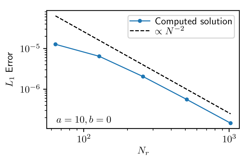
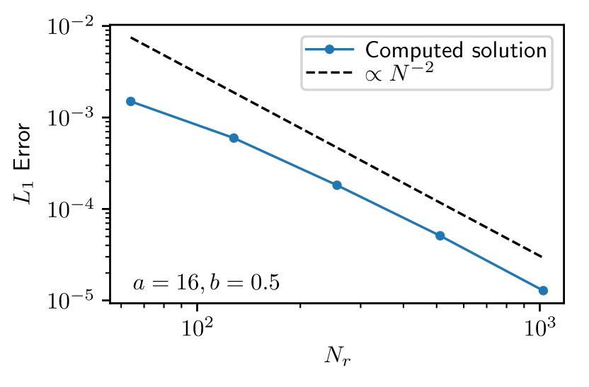
Refer to caption
Refer to caption
Figure 2.— Plotted are the L1subscript𝐿1L_{1} error measurements for the spherical wind problem found in Mignone (2014), as a function of number of radial zones (Nrsubscript𝑁𝑟N_{r}). These resolution tests were performed with two sets of parameters for the initial Gaussian density profiles used in Mignone, with his parameter pairs (a=10;b=0)formulae-sequence𝑎10𝑏0(a=10;b=0) (left panel) and (a=16;b=0.5)formulae-sequence𝑎16𝑏0.5(a=16;b=0.5) (right panel) (see Mignone 2014, his Eqs. 73 and 89). The solutions to this hydrodynamic wind problem are analytic, facilitating the demonstration of the rate of convergence to the correct solution. See text in §8.1 for a discussion.

7.5. Boundary Conditions

In spherical coordinates, certain unit vectors change sign discontinuously across coordinate singularities, i.e., the r^^𝑟\hat{r} and ϕ^^italic-ϕ\hat{\phi} unit vectors change sign across the origin in the radial direction and the θ^^𝜃\hat{\theta} and ϕ^^italic-ϕ\hat{\phi} unit vectors change sign across the axis in the polar direction. Following Baumgarte et al. (2013), we enforce parity conditions on the signs of the corresponding vector components in these ghost zones after copying the data from active zones. In the azimuthal direction, the grid at ϕ=2πitalic-ϕ2𝜋\phi=2\pi is mapped periodically to the grid at ϕ=0italic-ϕ0\phi=0, so that the data in active zone (i,j,Nϕ1)𝑖𝑗subscript𝑁italic-ϕ1(i,j,N_{\phi}-1) are mapped to ghost zone (i,j,1)𝑖𝑗1(i,j,-1) and, similarly, the data in active zone (i,j,0)𝑖𝑗0(i,j,0) are mapped to ghost zone (i,j,Nϕ)𝑖𝑗subscript𝑁italic-ϕ(i,j,N_{\phi}). In the polar direction at the axes, the data are periodically shifted in the azimuthal direction by Nϕ/2subscript𝑁italic-ϕ2N_{\phi}/2 zones as they are copied from the active zones into the ghost zones. Thus, the active zone (i,0,k)𝑖0𝑘(i,0,k) is mapped to the ghost zone (i,1,k)𝑖1superscript𝑘(i,-1,k^{\prime}), where k=(k+Nϕ/2)modNϕsuperscript𝑘modulo𝑘subscript𝑁italic-ϕ2subscript𝑁italic-ϕk^{\prime}=(k+N_{\phi}/2)\mod N_{\phi}. Finally, in the radial direction at the origin, the active-zone data are reflected in the polar direction and then periodically shifted as they are copied into the ghost zones. Thus, the active zone (0,j,k)0𝑗𝑘(0,j,k) is mapped to the ghost zone (1,j,k)1superscript𝑗superscript𝑘(-1,j^{\prime},k^{\prime}), where j=Nθ1jsuperscript𝑗subscript𝑁𝜃1𝑗j^{\prime}=N_{\theta}-1-j and ksuperscript𝑘k^{\prime} is as before. At the outer radial boundary, Fornax can employ a variety of boundary conditions, including outflow conditions with or without a diode restriction on the mass or radiation flux, Dirichlet and Neumann conditions, and arbitrary user-specified conditions.

8. Hydrodynamic Tests

8.1. Mignone Reconstruction Tests

We have taken special care in treating the reconstruction of quantities on the mesh and have formulated our reconstruction methods to be agnostic to choices of coordinates and mesh equidistance. As in Mignone (2014), we do this by forming our reconstruction expressions in terms of volume-averaged quantities and moments of the coordinates in each cell. The moments are calculated at start up for the given mesh and coordinates. In the radial direction, we have a uniform mesh in coordinate x1subscript𝑥1x_{1}, where the normal spherical radius r=rtsinh(x1/rt)𝑟subscript𝑟𝑡𝑠𝑖𝑛subscript𝑥1subscript𝑟𝑡r=r_{t}sinh(x_{1}/r_{t}), with rtsubscript𝑟𝑡r_{t} a constant parameter. We reconstruct quantities in x1subscript𝑥1x_{1}, i.e., we locally compute f(x1)𝑓subscript𝑥1f(x_{1}) to specify f𝑓f on the faces of each cell. The mesh in x1subscript𝑥1x_{1} is entirely uniform. We have no need of, and do not construct, f(r)𝑓𝑟f(r), where then the samples of f𝑓f would be non-uniformly distributed in r𝑟r. The same is true in the angular direction. Thus, we have no “non-equidistant” reconstruction and, therefore, our reconstructions yield the same results as Mignone (2014). For any choice of coordinates in any geometry, the method works the same and forms a consistent parabolic reconstruction from volume-averaged inputs.

To demonstrate the scaling of Fornax under this reconstruction regime, we have performed at various resolutions the L1subscript𝐿1L_{1} error radial/spherical wind test discussed in Mignone (2014). This hydrodynamic problem has an analytic solution (Mignone, his equation 89) and we have conducted the test for the Gaussian density profile provided in his Equation 73, with his parameters (a=10;b=0)formulae-sequence𝑎10𝑏0(a=10;b=0) and (a=16;b=0.5)formulae-sequence𝑎16𝑏0.5(a=16;b=0.5). Figure 2 depicts the associated convergence scaling for the two parameter sets, compared with quadratic (1N21superscript𝑁2\frac{1}{N^{2}}) behavior, and should be compared with Mignone’s Figure 10. Despite the fact this study was performed for a non-uniform radial grid, the expected scaling with resolution still emerges.
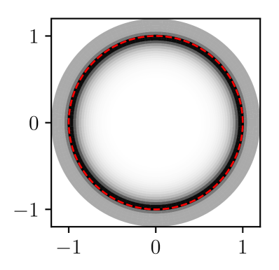
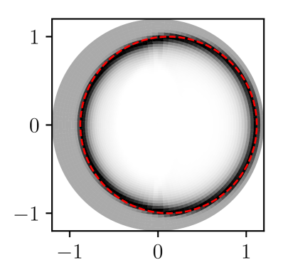
Refer to caption
Refer to caption
Figure 3.— Results of the three-dimensional Sedov blast wave test at time tfinal=1subscript𝑡final1t_{\mathrm{final}}=1. We plot the density, ρ𝜌\rho, for the on-axis (left) and off-axis (right) blast waves along a slice at y=0𝑦0y=0 using a linear gray color scale from ρ=0𝜌0\rho=0 (white) to ρ=3𝜌3\rho=3 (black). The analytic shock radius location, rshsubscript𝑟shr_{\mathrm{sh}}, is overplotted (red dashed line). Small-scale axis artifacts are apparent in the off-axis version, but the solution remains fairly spherical even though the blast is nowhere aligned to the grid.
Refer to caption
Refer to caption
Figure 4.— Same as Figure 3 but for the internal energy density, u𝑢u, which is plotted using a linear gray color scale from u=0𝑢0u=0 (white) to u=0.25𝑢0.25u=0.25 (black). Small-scale axis artifacts are less apparent, since pressure gradients tend to get smoothed out behind the shock front.

8.2. Centered and Off-Centered Sedov Blast Wave

A standard test is the classical self-similar blast wave of Sedov (1959) describing, e.g., the initial energy-conserving phase of a supernova remnant. The problem consists of a stationary background medium with uniform density ρ1subscript𝜌1\rho_{1} and near-zero pressure P1subscript𝑃1P_{1} into which a prescribed blast energy E1subscript𝐸1E_{1} is deposited. Since P10subscript𝑃10P_{1}\approx 0, the solution depends on only the two parameters ρ1subscript𝜌1\rho_{1} and E1subscript𝐸1E_{1}, it follows that the radius, r𝑟r, and the time since explosion, t𝑡t, are related by a dimensionless similarity variable, ξ𝜉\xi. Thus, it can be shown that the position of the shock radius is given by

rsh(t)=ξ0(E1t2ρ1)1/5,subscript𝑟sh𝑡subscript𝜉0superscriptsubscript𝐸1superscript𝑡2subscript𝜌115r_{\mathrm{sh}}(t)=\xi_{0}\left(\frac{E_{1}t^{2}}{\rho_{1}}\right)^{1/5}\,, (39)

where ξ01.033subscript𝜉01.033\xi_{0}\approx 1.033 for an adiabatic equation of state with γ=1.4𝛾1.4\gamma=1.4. Following Kamm & Timmes (2007), we set the dimensionless inputs to γ=1.4𝛾1.4\gamma=1.4, ρ1=1subscript𝜌11\rho_{1}=1, P1=4×10¹³subscript𝑃14superscript1013P_{1}=4\times 10^{-13}, and E1=0.851072subscript𝐸10.851072E_{1}=0.851072 such that the outer blast radius is at rsh=1subscript𝑟sh1r_{\mathrm{sh}}=1 at time t=1𝑡1t=1. We use a three-dimensional spherical dendritic grid with radial extent out to rmax=1.2subscript𝑟max1.2r_{\mathrm{max}}=1.2 and a resolution of 64×64×128646412864\times 64\times 128 zones. The radial grid spacing is constant in the interior with Δr0.01Δ𝑟0.01\Delta r\approx 0.01 out to r0.3𝑟0.3r\approx 0.3, then smoothly transitions to logarithmic spacing out to rmaxsubscript𝑟maxr_{\mathrm{max}}.

For our first test, we deposit all of E1subscript𝐸1E_{1} in the zones surrounding the origin. As expected, the subsequent blast is aligned with the grid and maintains perfect spherical symmetry. Next, we deposit the same energy in the zones closest to the x𝑥x-axis at r=0.12𝑟0.12r=0.12 so that the blast is off-axis. This time the blast is not aligned with the grid and must cross the polar axis as it expands. Figures 3 and 4 compare the density and internal energy of the on- and off-axis blast waves, respectively. There are small-scale axis artifacts in the density in the off-axis version of the blast wave, but the blast wave remains fairly spherical despite being nowhere aligned with the spherical grid. The scale of the artifacts is smaller in the internal energy, since pressure variations tend to be smoothed out behind the shock where the pressure is large.

Overall, this test demonstrates that the internal geometric boundary conditions at the origin and polar axes are correctly applied. The artifacts at the axes are likely due to small errors in reconstruction in the azimuthal direction with our dendritic grid. The direction of the polar and azimuthal coordinate vectors is divergent at the polar axis, hence angular variations in the data there can only be resolved by a correspondingly convergent grid. In the limit of a locally “planar” flow across the poles, the rapid azimuthal variation comes entirely from the coordinates themselves, not from the data, although these variations must average to zero. Our dendritic grid deresolves this rapid angular variation, introducing first-order errors due to monotonicity contraints. However, these artifacts are confined to a narrow polar axis region and do not adversely contaminate the solution elsewhere.

8.3. Sod Shock Tube

To demonstrate the shock-capturing capabilities of Fornax, we consider the classical shock-tube test of Sod (1978). The initial data consists of two states:

(ρ,P)={(1.0,1.0),if x<0,(0.125,0.1),otherwise.𝜌𝑃cases1.01.0if 𝑥00.1250.1otherwise(\rho,P)=\begin{cases}(1.0,1.0),&\textrm{if }x<0\,,\\ (0.125,0.1),&\textrm{otherwise}\,.\end{cases} (40)

The initial velocity is set to zero. For this test we adopt an adiabatic equation of state with index γ=1.4𝛾1.4\gamma=1.4.

This test is not particularly challenging for modern HRSC codes, but it is nevertheless interesting because it exhibits all fundamental hydrodynamical waves. The exact solution consists of a left propagating rarefaction wave, a right propagating contact discontinuity, and a right propagating shock.

Refer to caption
Figure 5.— Density, pressure, and velocity (left, middle, and right panels respectively) for the Sod test. The solid line is the analytic solution, while the dots show the Fornax results at a resolution of 646464 grid points. All of the key features of the solution are correctly captured, but the contact wave is smeared over 4similar-toabsent4{\sim}4 grid points.

Figure 5 shows the analytic solution and the results from Fornax using a coarse mesh of 64 points. The code correctly captured all of the waves. The shock wave is sharply captured within 2similar-toabsent2{\sim}2 grid points, while the contact wave is smeared over 4similar-toabsent4{\sim}4 grid points.

8.4. Double Mach Reflection

To test the sensitivity of the Fornax code to ithe numerical diffusion of contact waves, we perform the classic double Mach reflection test of Woodward & Collela (1984). This test consists of a Mach-10 oblique shock through air (γ=1.4𝛾1.4\gamma=1.4), inclined with respect to a reflecting boundary in which the incident and reflected shocks then interact to produce a triple point. In the space between the reflected shock and the contact discontinuity, an upward-directed jet should form along the slip surface, but if the numerical dissipation of the contact wave is too high, the formation of this jet will be suppressed. We use a two-dimensional grid of 520×160520160520\times 160 zones over the domain (x,y)[0,3.25]×[0,1]𝑥𝑦03.2501(x,y)\in[0,3.25]\times[0,1] and position an oblique shock at x0=1/6subscript𝑥016x_{0}=1/6 inclined at an angle α=π/3𝛼𝜋3\alpha=\pi/3 with respect to the x𝑥x-axis. The pre-shock state is given by (ρ,P,vx,vy)R=(1.4,1,0,0)subscript𝜌𝑃subscript𝑣𝑥subscript𝑣𝑦R1.4100(\rho,P,v_{x},v_{y})_{\mathrm{R}}=(1.4,1,0,0) and the post-shock state by (ρ,P,vx,vy)L=(8,116.5,8.25sinα,8.25cosα(\rho,P,v_{x},v_{y})_{\mathrm{L}}=(8,116.5,8.25\sin\alpha,-8.25\cos\alpha). The left x𝑥x-boundary is held fixed at the post-shock state and outflow conditions are imposed at the right x𝑥x-boundary. At the lower y𝑦y-boundary, the post-shock state is fixed for xx0𝑥subscript𝑥0x\leq x_{0} and reflecting boundary conditions are imposed for x>x0𝑥subscript𝑥0x>x_{0}. Meanwhile, at the upper y𝑦y-boundary, the time-dependent shock position, xs=x0+y/tanα+10t/sinαsubscript𝑥𝑠subscript𝑥0𝑦𝛼10𝑡𝛼x_{s}=x_{0}+y/\tan\alpha+10t/\sin\alpha, is used to set either the post-shock state (xxs𝑥subscript𝑥𝑠x\leq x_{s}) or the pre-shock state (x>xs𝑥subscript𝑥𝑠x>x_{s}).

Refer to caption
Figure 6.— Results at time tfinal=0.2subscript𝑡final0.2t_{\mathrm{final}}=0.2 of the double Mach reflection test. We use a resolution of 520×160520160520\times 160 Cartesian grid zones and plot 30 linearly-spaced contours of the density. On the right-hand side, the incident and reflected shocks form a triple point, below which an upward-directed jet is formed along the slip surface at y=0𝑦0y=0.

Figure 6 shows the evolved system at tfinal=0.2subscript𝑡final0.2t_{\mathrm{final}}=0.2 using 30 linearly-spaced contours of the density. The features at the various shock fronts remain sharp, and in the region below the triple point a small upward-directed jet is indeed produced along the slip surface. This indicates that numerical dissipation of the contact wave is well-controlled in Fornax.

8.5. Rayleigh-Taylor Instability

8.5.1 Two-Dimensional Rayleigh-Taylor Test

Here, we study the linear and non-linear development of the Rayleigh-Taylor instability in 2-d. The initial data describes an unstably stratified fluid with

ρ={ρhif z0,ρlotherwise.𝜌casessubscript𝜌if 𝑧0subscript𝜌𝑙otherwise\rho=\begin{cases}\rho_{h}&\textrm{if }z\geq 0\,,\\ \rho_{l}&\textrm{otherwise}\,.\\ \end{cases} (41)

The gravitational acceleration g=1/2𝑔12g=1/2 is parallel to the z𝑧z axis, and ρh=2subscript𝜌2\rho_{h}=2, ρl=1subscript𝜌𝑙1\rho_{l}=1, so that the Atwood number A=(ρhρl)/(ρh+ρl)𝐴subscript𝜌subscript𝜌𝑙subscript𝜌subscript𝜌𝑙A=(\rho_{h}-\rho_{l})/(\rho_{h}+\rho_{l}) is 1/3131/3. The boundary conditions are reflective for z=±1𝑧plus-or-minus1z=\pm 1 and periodic for x=±1/2𝑥plus-or-minus12x=\pm 1/2. The initial pressure is chosen to ensure hydrostatic equilibrium:

P(z)=P(1)+1zρgdz,𝑃𝑧𝑃1superscriptsubscript1𝑧𝜌𝑔differential-d𝑧P(z)=P(-1)+\int_{-1}^{z}\rho\,g\,\mathrm{d}z\,, (42)

with P(1)=10/7+1/4𝑃110714P(-1)=10/7+1/4. For this test we adopt an adiabatic equation of state with index γ=1.4𝛾1.4\gamma=1.4.

At time t=0𝑡0t=0 the interface between the two fluid components is perturbed to be

h(x)=h0cos(κx),𝑥subscript0𝜅𝑥h(x)=h_{0}\cos(\kappa x)\,, (43)

with h0=0.01subscript00.01h_{0}=0.01 and κ=4π𝜅4𝜋\kappa=4\pi. The sharp interface is then smoothed into an hyperbolic tangent profile with characteristic length 0.0050.0050.005.

According to analytic theory hh should evolve according to the following equation:

h(x,t)=h0cosh(Aκgt)cos(κx).𝑥𝑡subscript0𝐴𝜅𝑔𝑡𝜅𝑥h(x,t)=h_{0}\,\cosh(\sqrt{A\kappa g}\,t)\,\cos(\kappa x)\,. (44)
Refer to caption
Figure 7.— Amplitude of the interface perturbation for the single mode 2-d Rayleigh-Taylor test. We show results from different resolutions and the expected growth rate from analytic theory. We find perfect agreement with linear theory up to t1.75similar-to-or-equals𝑡1.75t\simeq 1.75, when secondary instabilities start to appear in the flow and the dynamics becomes fully nonlinear.

We perform simulations with resolutions ranging from 64×1286412864\times 128 to 1024×2048102420481024\times 2048. We track the mixing of the two fluid components by means of a passive scalar tracer. This is initialized to be ρρl𝜌subscript𝜌𝑙\rho-\rho_{l}, so that the value 111 corresponds to the heavy fluid, while the value 00 corresponds to the light fluid. We track the growth of the initial perturbation by locating the 0.990.990.99 isocontour of the tracer. Figure 7 shows the perturbation amplitude, normalized by its initial value, and the prediction from analytic theory (Eq. 44).

At low resolution, the perturbations grow exponentially from t=0𝑡0t=0, but the growth rate is somewhat smaller than that predicted by analytic theory. The slower growth rate at low resolution is not unexpected and is due to the numerical viscosity, which modifies the Rayleigh-Taylor dispersion relation (Dimonte et al. 2004; Murphy & Burrows 2008a). We speculate that the reason why the initial perturbations grow exponentially at low resolution is that they are not well resolved. At higher resolution the correct cosh\cosh time dependence is recovered and the agreement with linear theory is excellent up to time t1.75similar-to-or-equals𝑡1.75t\simeq 1.75, when the Rayleigh-Taylor plumes start to break and rolls develop.

Refer to caption
Figure 8.— Passive tracer concentration for the single mode 2-d Rayleigh-Taylor test at three representative times. The resolution is 1024×2048102420481024\times 2048. During the linear phase of the instability, up to t1.75similar-to-or-equals𝑡1.75t\simeq 1.75, the contact discontinuity is well preserved and there is no spurious mixing of the two fluid phases. Secondary instabilities, seeded by the numerical noise, appear at later times, during the non-linear phase of the evolution.

During the non-linear phase of the evolution, secondary Rayleigh-Taylor and Kelvin-Helmholtz instabilities appear (Fig. 8). These are seeded by the numerical noise and their detailed morphology, in the absence of explicit dissipation, is known to be dependent on the details of the numerical scheme (Liska & Wendroff 2003a). Despite the presence of these features, Fornax is able to preserve the sharp discontinuity in the fluid tracer. Artificial mixing between the two fluid components is only present in the Rayleigh-Taylor rolls, where the flow develops features on scales comparable to that of the grid.

8.5.2 Three-Dimensional Rayleigh-Taylor Test

Neutrino-driven convection plays a central role in the explosion mechanism of CCSNe (Burrows 2013; Radice et al. 2017; Burrows et al. 2018; Vartanyan et al. 2018). In this section, we benchmark Fornax for the modeling of convective flows by studying the nonlinear development of the Rayleigh-Taylor instability in 3-d. We consider the setup introduced by Dimonte et al. (2004), for which the dynamics is dominated by mode couplings.

The computational domain is a box with L/2<x,y<L/2formulae-sequence𝐿2𝑥𝑦𝐿2-L/2<x,y<L/2, L<z<L𝐿𝑧𝐿-L<z<L, where L=10𝐿10L=10 in arbitrary units. We consider a constant vertical gravitational acceleration g:=gz=2assign𝑔subscript𝑔𝑧2g:=-g_{z}=2, and we prepare initial conditions with density stratification

ρ(z)=ρ0(1γ1γρ0gzP0)1γ1𝜌𝑧subscript𝜌0superscript1𝛾1𝛾subscript𝜌0𝑔𝑧subscript𝑃01𝛾1\rho(z)=\rho_{0}\left(1-\frac{\gamma-1}{\gamma}\frac{\rho_{0}gz}{P_{0}}\right)^{\frac{1}{\gamma-1}}\, (45)

where γ=5/3𝛾53\gamma=5/3,

ρ0={ρhif z0,ρlotherwise,subscript𝜌0casessubscript𝜌if 𝑧0subscript𝜌𝑙otherwise\rho_{0}=\begin{cases}\rho_{h}&\textrm{if }z\geq 0\,,\\ \rho_{l}&\textrm{otherwise}\,,\end{cases} (46)

and p0=2π(ρh+ρl)gLsubscript𝑝02𝜋subscript𝜌subscript𝜌𝑙𝑔𝐿p_{0}=2\pi(\rho_{h}+\rho_{l})gL. We set ρh=3subscript𝜌3\rho_{h}=3 and ρl=1subscript𝜌𝑙1\rho_{l}=1, so that the Atwood number A=(ρhρl)/(ρh+ρl)𝐴subscript𝜌subscript𝜌𝑙subscript𝜌subscript𝜌𝑙A=(\rho_{h}-\rho_{l})/(\rho_{h}+\rho_{l}) is 1/2121/2. The initial pressure is set to

P=P0(ρρ0)γ,𝑃subscript𝑃0superscript𝜌subscript𝜌0𝛾P=P_{0}\left(\frac{\rho}{\rho_{0}}\right)^{\gamma}\,, (47)

which ensures that the initial conditions are in hydrostatic equilibrium. We track the concentration of the “heavy” fluid by evolving a passive scalar field fhsubscript𝑓f_{h} initialized to be one for positive z𝑧z and zero otherwise. We assume periodicity in the x𝑥x and y𝑦y direction and hydrostatic boundary conditions at z=±L𝑧plus-or-minus𝐿z=\pm L. We use uniform grids and label our simulations by the number of grid points in the x𝑥x direction so that, e.g., the N128 run has a resolution of 128×128×256128128256128\times 128\times 256 points.

At time t=0𝑡0t=0 the interface between the two fluid components is perturbed to be

h(x,y)=1H8kx2+ky216[a𝐤cos(kxX)cos(kyY)+b𝐤cos(kxX)sin(kyY)+c𝐤sin(kxX)cos(kyY)+d𝐤sin(kxX)sin(kyY)],𝑥𝑦1𝐻subscript8superscriptsubscript𝑘𝑥2superscriptsubscript𝑘𝑦216delimited-[]subscript𝑎𝐤subscript𝑘𝑥𝑋subscript𝑘𝑦𝑌subscript𝑏𝐤subscript𝑘𝑥𝑋subscript𝑘𝑦𝑌subscript𝑐𝐤subscript𝑘𝑥𝑋subscript𝑘𝑦𝑌subscript𝑑𝐤subscript𝑘𝑥𝑋subscript𝑘𝑦𝑌\begin{split}h(&x,y)=\frac{1}{H}\sum_{8\leq k_{x}^{2}+k_{y}^{2}\leq 16}\Big{[}a_{\mathbf{k}}\cos(k_{x}X)\cos(k_{y}Y)+\\ &b_{\mathbf{k}}\cos(k_{x}X)\sin(k_{y}Y)+c_{\mathbf{k}}\sin(k_{x}X)\cos(k_{y}Y)+\\ &d_{\mathbf{k}}\sin(k_{x}X)\sin(k_{y}Y)\Big{]}\,,\end{split} (48)

where X=2πx/L𝑋2𝜋𝑥𝐿X=2\pi x/L and Y=2πy/L𝑌2𝜋𝑦𝐿Y=2\pi y/L. The coefficients a𝐤subscript𝑎𝐤a_{\mathbf{k}}, b𝐤subscript𝑏𝐤b_{\mathbf{k}}, c𝐤subscript𝑐𝐤c_{\mathbf{k}}, and d𝐤subscript𝑑𝐤d_{\mathbf{k}} are sampled from a uniform distribution taking values between 11-1 and 111, boundary excluded. H𝐻H is a normalization coefficient that we adjust after having sampled a𝐤subscript𝑎𝐤a_{\mathbf{k}}, b𝐤subscript𝑏𝐤b_{\mathbf{k}}, c𝐤subscript𝑐𝐤c_{\mathbf{k}}, and d𝐤subscript𝑑𝐤d_{\mathbf{k}} so that hrms=3×10⁴Lsubscriptrms3superscript104𝐿h_{\rm rms}=3\times 10^{-4}L. We remark that we use the same initial conditions for all of our simulations, while Dimonte et al. (2004) used a different number of modes in their initial perturbation depending on the resolution. We also use the same realization of the coefficients in Equation (48) for all the simulations presented in this section. In this way, the convergence of our numerical results can be better assessed.

When constructing the perturbed initial data, we compute the cell-averaged density, internal energy, and heavy-fluid concentration, i.e., the quantities evolved by the finite-volume scheme in Fornax, by numerically integrating the profiles discussed above on an auxiliary mesh with 50 times higher resolution than the base grid in each direction.
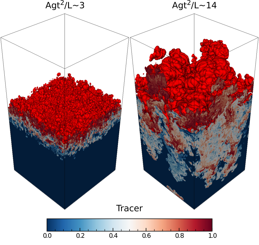
Refer to caption
Figure 9.— Passive tracer concentration for the multi-mode 3-d Rayleigh-Taylor test at two representative times. Red values indicate higher concentration for the “heavy” fluid. The red surface is the 99% isocontour of the concentration. The resolution is 512×512×10245125121024512\times 512\times 1024.

The initial perturbations generate small buoyant bubbles that interact and grow into larger bubbles as the system evolves, as shown in Figure 9. We find that there is significant mixing between the two fluids. This is evidenced by the intermediate values taken by fhdelimited-⟨⟩subscript𝑓\langle f_{h}\rangle (see Eq. 49 below), especially in the buoyant bubbles which entrain a significant amount of the heavy fluid. At late times, the topology of the interface between the two fluids becomes non-trivial and we observe the detachment of some of the bubbles.
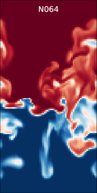
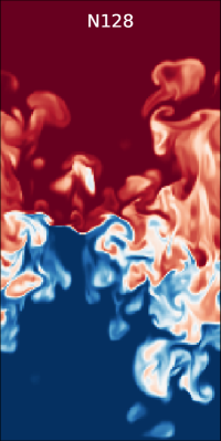
Refer to caption
Refer to caption
Refer to caption
Refer to caption
Figure 10.— Passive tracer concentration in the xz𝑥𝑧xz-plane for the multi-mode 3-d Rayleigh-Taylor test at time Agt2/L14similar-to-or-equals𝐴𝑔superscript𝑡2𝐿14Agt^{2}/L\simeq 14 for different resolutions. The dominant features of the flow are in qualitative agreement between the different resolutions, despite the highly non-linear nature of the flow at this time.

The entrainment of the heavy fluid in the buoyant bubbles and of the light fluid in the sinking plumes is not strongly dependent on the resolution, but they appear to grow slightly with resolution, as shown in Figure 10. This is presumably due to the higher effective Reynolds numbers achieved in the best resolved simulations. Note that we do not include an explicit viscosity in these simulations, consequently the dissipation scale is a multiple of the grid scale. At high resolutions secondary instabilities with smaller wave number and faster growth rates are allowed to develop. Their presence might explain the increase in the entrainment with resolution. Despite these quantitative differences we find a remarkable qualitative agreement between the different resolutions with the gross flow feature captured even at the lowest resolution of 64×64×128646412864\times 64\times 128.

Refer to caption
Refer to caption
Figure 11.— Horizontally-averaged concentration of the heavy fluid at an early time (Agt2/L3similar-to-or-equals𝐴𝑔superscript𝑡2𝐿3Agt^{2}/L\simeq 3; left panel) and at a late time (Agt2/L14similar-to-or-equals𝐴𝑔superscript𝑡2𝐿14Agt^{2}/L\simeq 14; right panel). The blue points are the experimental data extracted from Dimonte et al. (2004), the solid lines are Fornax calculations at different resolutions. We find good agreement between the numerical and the experimental data.

Following Dimonte et al. (2004) we compute the horizontally-averaged concentration of the heavy fluid

fh=1L2fhdxdydelimited-⟨⟩subscript𝑓1superscript𝐿2double-integralsubscript𝑓differential-d𝑥differential-d𝑦\langle f_{h}\rangle=\frac{1}{L^{2}}\iint f_{h}\,\mathrm{d}x\,\mathrm{d}y (49)

and we define as the bubble penetration depth hbsubscript𝑏h_{b} the z𝑧z value at which fhdelimited-⟨⟩subscript𝑓\langle f_{h}\rangle reaches 99%. The profile of fhdelimited-⟨⟩subscript𝑓\langle f_{h}\rangle is observed to be self-similar during the non-linear development of the Rayleigh-Taylor instability. We show the profile of fhdelimited-⟨⟩subscript𝑓\langle f_{h}\rangle obtained with Fornax at two representative times in Figure 11. Also shown are the experimental results obtained by Dimonte et al. (2004), as reported in that paper. This figure should be contrasted with Figure 7 of Dimonte et al. (2004). We find good agreement between the Fornax results and the experimental data. The agreement improves as the resolution increases, with the exception of a spike appearing at late times in the N512 data around z/hb1similar-to-or-equals𝑧subscript𝑏1z/h_{b}\simeq-1. This is caused by the interaction of some of the down-falling plumes with the boundary at the bottom of the simulation box.
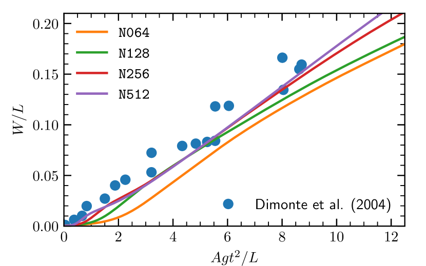
Refer to caption
Figure 12.— Mixing degree as a function of the dimensionless time Agt2/L𝐴𝑔superscript𝑡2𝐿Agt^{2}/L. The blue points are the experimental data extracted from Dimonte et al. (2004). The other lines are results from Fornax calculations. We find that Fornax agrees well with the experimental data predicting the right growth rate of the instability in the non-linear regime.

Following Andrews & Spalding (1990) and Dimonte et al. (2004), we quantify the mixing degree between the heavy and the light fluid with the metric

W=fh(1fh)dz.𝑊delimited-⟨⟩subscript𝑓1delimited-⟨⟩subscript𝑓differential-d𝑧W=\int\langle f_{h}\rangle\left(1-\langle f_{h}\rangle\right)\,\mathrm{d}z\,. (50)

Our results are shown in Figure 12. The growth rate of the instability in the nonlinear phase is proportional to Agt2/L𝐴𝑔superscript𝑡2𝐿Agt^{2}/L, as predicted by theoretical models and confirmed by experimental results (Dimonte et al. 2004). The progression of the mixing between the two fluids as computed by Fornax agrees well with the experimental results reported in Dimonte et al. (2004). We find that Fornax compares favorably to the other Eulerian codes presented in Dimonte et al. (2004), such as FLASH. Fornax yields results of comparable in quality to those of Arbitrary Lagrangian-Eulerian (ALE) codes with interface reconstruction methods (cf. Fig. 8 of Dimonte et al. 2004). That said we want to remark that, as documented in Dimonte et al. (2004) and as we have confirmed in preliminary calculations, the exact rate of mixing between the two fluids depends to some extent on the spectrum and the character of the initial perturbations. We have not fine-tuned the initial conditions of our simulations to match the experimental data.666We adopted the initial conditions of Dimonte et al. (2004) for the N064 resolution, and we have kept them fixed as we increased the resolution. Nevertheless, we cannot exclude the possibility that the better agreement with the experimental data of Fornax compared to the results from the other Eulerian codes presented in Dimonte et al. (2004) is due partly to the different choice of initial conditions.
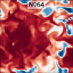
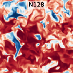
Refer to caption
Refer to caption
Refer to caption
Refer to caption
Figure 13.— Passive tracer concentration in the xy𝑥𝑦xy-plane for the multi-mode 3-d Rayleigh-Taylor test at time Agt2/L14similar-to-or-equals𝐴𝑔superscript𝑡2𝐿14Agt^{2}/L\simeq 14 for different resolutions. Note the appearance of small-scale flow structures as the resolution is increased.

We analyze the character of the fluctuations in fhsubscript𝑓f_{h} on the original interface at z=0𝑧0z=0 at an advanced time Agt2/L14similar-to-or-equals𝐴𝑔superscript𝑡2𝐿14Agt^{2}/L\simeq 14 (Fig. 13). We find good qualitative agreement between the two highest resolution simulations. However, there are quantitative differences. Particularly noticeable is the appearance of smaller scale fluid features as the resolution is increased. This is expected since we do not include an explicit viscosity in our simulations. Instead, the dissipation scale is related to the grid resolution, so that higher resolution simulations have a larger effective Reynolds number.
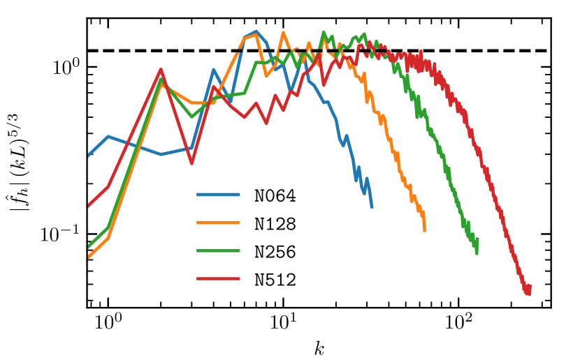
Refer to caption
Figure 14.— Power-spectra of the heavy fluid concentration on the initial interface z=0𝑧0z=0 at Agt2/L14similar-to-or-equals𝐴𝑔superscript𝑡2𝐿14Agt^{2}/L\simeq 14. The spectra are normalized to have unit norm and then compensated by k5/3superscript𝑘53k^{5/3} so that regions with Kolmogorov scaling appear flat. As the resolution is increased, a progressively larger extent of the inertial range is recovered.

We quantify this observation by computing the power spectrum of fhsubscript𝑓f_{h} on the original interface at z=0𝑧0z=0 at Agt2/L14similar-to-or-equals𝐴𝑔superscript𝑡2𝐿14Agt^{2}/L\simeq 14. We define the 2-d spectrum of fhsubscript𝑓f_{h} as

f^h(𝐤)=fh(𝐱)|z=0exp(2πi𝐤𝐱L)d2𝐱subscript^𝑓𝐤evaluated-atdouble-integralsubscript𝑓𝐱𝑧02𝜋i𝐤𝐱𝐿superscriptd2𝐱\hat{f}_{h}(\mathbf{k})=\iint f_{h}(\mathbf{x})|_{z=0}\exp\left(2\pi\mathrm{i}\mathbf{k}\cdot\frac{\mathbf{x}}{L}\right)\mathrm{d}^{2}\mathbf{x} (51)

and the 1D spectrum as

f^h(k)=δ(𝐤k)f^h(𝐤)d2𝐤.subscript^𝑓𝑘double-integral𝛿𝐤𝑘subscript^𝑓𝐤superscriptd2𝐤\hat{f}_{h}(k)=\iint\delta(\mathbf{k}-k)\,\hat{f}_{h}(\mathbf{k})\,\mathrm{d}^{2}\mathbf{k}\,. (52)

Because of the periodic boundary conditions, the 2-d spectrum is nontrivial only for 𝐤=(kx,ky)𝐤subscript𝑘𝑥subscript𝑘𝑦\mathbf{k}=(k_{x},k_{y}) with kxsubscript𝑘𝑥k_{x}, kysubscript𝑘𝑦k_{y} integers. When computing the 1D spectrum, we convert the integral into a weighted summation following Eswaran & Pope (1988), i.e., we set

f^h(k)=2πkNk𝐤=kf^h(𝐤),subscript^𝑓𝑘2𝜋𝑘subscript𝑁𝑘subscriptnorm𝐤𝑘subscript^𝑓𝐤\hat{f}_{h}(k)=\frac{2\pi k}{N_{k}}\sum_{\|\mathbf{k}\|=k}\hat{f}_{h}(\mathbf{k})\,, (53)

where Nksubscript𝑁𝑘N_{k} is the number of modes with κ1/2<𝐤<κ+1/2𝜅12norm𝐤𝜅12\kappa-1/2<\|\mathbf{k}\|<\kappa+1/2. Our results are shown in Figure 14.

We find that the spectrum appears converged for k2similar-to𝑘2k\sim 2, as could have been anticipated by looking at the dipolar component of the oscillations in Figure 13. However, we find that fluctuations with scales k10similar-to𝑘10k\sim 10 are progressively suppressed as the resolution increases. The lack of convergence at these intermediate scales can be attributed to nonlinear mode coupling becoming stronger as the effective Reynolds number of the simulations increases. At smaller scales, the flow becomes self-similar and develops an inertial range. We find that the power spectrum follows the scaling expected from Kolmogorov’s theory of turbulence for a passively advected scalar field, i.e., |f^h|k5/3proportional-tosubscript^𝑓superscript𝑘53|\hat{f}_{h}|\propto k^{-5/3} (Pope 2000). We also find that, as the resolution increases, a progressively larger part of the inertial range is uncovered. At scales of less than 5similar-toabsent5{\sim}5 grid points the power spectrum drops due to the direct effect of numerical viscosity.

8.6. Kelvin-Helmholtz Instability

The Kelvin-Helmholtz (KH) instability is a two-dimensional instability arising from a velocity shear within a fluid. The instability results in vorticity, which can cascade into turbulence. As such, it is of particular interest in the study of core-collapse supernova, where cascading turbulence can contribute to shock revival.

We consider a fluid over the rectangular domain within x[0,4]𝑥04x\in[0,4] and z[0,2]𝑧02z\in[0,2], with a setup similar to that found in Lecoanet et al. (2016) and with a density jump characterized by the initial conditions below. We conduct tests at low, medium, high resolutions, defined as 512×256512256512\times 256, 1024×51210245121024\times 512, and 2048×1024204810242048\times 1024, respectively.

ρ𝜌\displaystyle\rho =1+δρ2ρ0[tanh(zz1a)tanh(zz2a)]absent1𝛿𝜌2subscript𝜌0delimited-[]tanh𝑧subscript𝑧1𝑎tanh𝑧subscript𝑧2𝑎\displaystyle=1+\frac{\delta\rho}{2\rho_{0}}\,\left[\mathrm{tanh}\left(\frac{z-z_{1}}{a}\right)-\mathrm{tanh}\left(\frac{z-z_{2}}{a}\right)\right] (54a)
v𝑣\displaystyle v =u0×[tanh(zz1a)tanh(zz2a)]absentsubscript𝑢0delimited-[]tanh𝑧subscript𝑧1𝑎tanh𝑧subscript𝑧2𝑎\displaystyle=u_{0}\times\left[\mathrm{tanh}\left(\frac{z-z_{1}}{a}\right)-\mathrm{tanh}\left(\frac{z-z_{2}}{a}\right)\right] (54b)
w𝑤\displaystyle w =Asin(πx)×[exp((zz1)2σ2)+exp((zz2)2σ2)],absentAsin𝜋𝑥delimited-[]expsuperscript𝑧subscript𝑧12superscript𝜎2expsuperscript𝑧subscript𝑧22superscript𝜎2\displaystyle=\mathrm{A}\,\mathrm{sin}(\pi x)\times\left[\mathrm{exp}\left(-\frac{(z-z_{1})^{2}}{\sigma^{2}}\right)+\mathrm{exp}\left(-\frac{(z-z_{2})^{2}}{\sigma^{2}}\right)\right]\,, (54c)

with a=0.05𝑎0.05a=0.05, σ=0.2𝜎0.2\sigma=0.2, z1=0.5subscript𝑧10.5z_{1}=0.5, and z2=1.5subscript𝑧21.5z_{2}=1.5. We define v𝑣v as the velocity in the x𝑥x-direction and w𝑤w as the velocity in the z𝑧z-direction.

The initial amplitude, A𝐴A, of the perturbation in the vertical (z𝑧z-direction) velocity (w𝑤w) is set to 0.01, and the initial density perturbation, δρ/ρ0𝛿𝜌subscript𝜌0\delta\rho/\rho_{0}, is set to 1.0. The initial pressure P0subscript𝑃0P_{0} is 10, the initial lateral velocity constant, u0subscript𝑢0u_{0}, is set to 1.0, and the initial density ρ𝜌\rho is set to 1.0. We assume an adiabatic gas with adiabatic index γ=5/3𝛾53\gamma=5/3. The resulting Mach number (M𝑀M) is 0.25similar-toabsent0.25{\sim}0.25, consistent with quasi-incompressible flow. As is often done in KH instability tests, we ignore gravity.
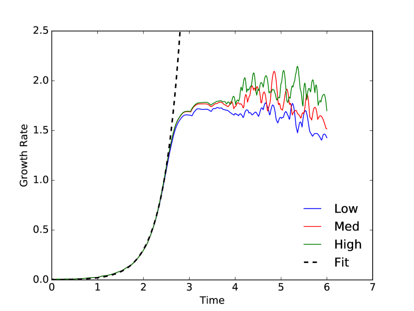
Refer to caption
Figure 15.— In the context of the Kelvin-Helmholtz study, the growth rate of the maximum of w𝑤w, the velocity in the z𝑧z-direction as a function of time for three different resolutions: low (blue), medium (red), and high (green). In thick dashed black we plot the best fitting exponential to the growth rate in the linear regime, which breaks down at t2.6similar-to𝑡2.6t\sim 2.6.

In Figure 15, we plot as a function of time the growth rate of the maximum of w𝑤w, the velocity in the z𝑧z-direction. The linear growth phase of the Kelvin-Helmholtz instability lasts until t2.6similar-to𝑡2.6t\sim 2.6 (in our dimensionless units) for all models, which evolve virtually identically, independent of resolution, until the nonlinear regime.

Refer to caption
Refer to caption
Refer to caption
Figure 16.— Two-dimensional density evolution of the Kelvin-Helmholtz instability over the grid at 3 different times: t=0𝑡0t=0, our initial condition (top), t=3𝑡3t=3 (middle), and t=6𝑡6t=6 (bottom). The vertical velocity perturbations translate to density perturbations, forming vortices at later times.

In Figure 16, we plot the 2-d density evolution at three times (t=0,3,6𝑡036t=0,3,6 in dimensionless units) over our grid. Initial density perturbations evolve to form characteristic vortices at later times.

8.7. Liska-Wendroff Implosion Test
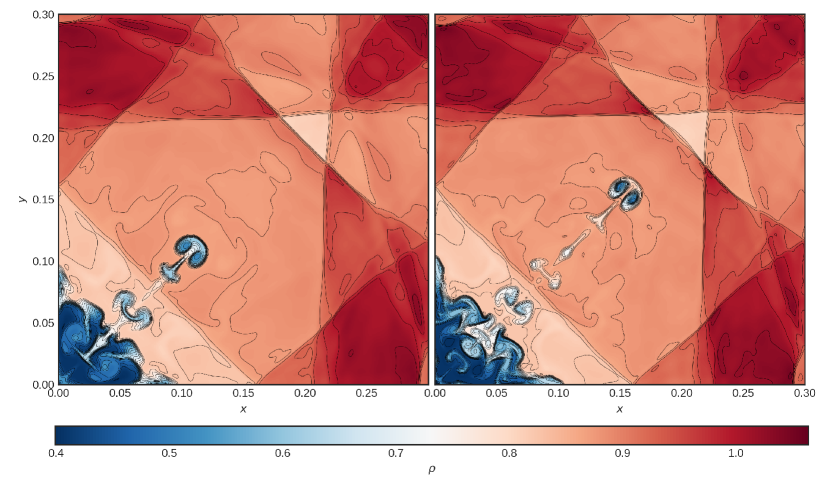
Refer to caption
Figure 17.— Results of the 2-d implosion problem of Liska & Wendroff (2003b) at t=2.5𝑡2.5t=2.5 on a 400×400400400400\times 400 mesh using linear (left) and parabolic (right) reconstruction methods. Contours are shown for ρ=[0.35,1.1]𝜌0.351.1\rho=[0.35,1.1] at 31 equidistant values and are exactly symmetric about y=x𝑦𝑥y=x. The longer jet in the results at right reflect the lower numerical diffusion characteristic of parabolic relative to linear reconstruction methods.
Refer to caption
Figure 18.— Results of the 2-d implosion problem of Liska & Wendroff (2003) at t=2.5𝑡2.5t=2.5 on a 1600×1600160016001600\times 1600 mesh using parabolic reconstruction. At this very high resolution, the vortices at the tip of the jet have propagated into the upper right corner and reflected, running back along the top and right sides. The overall structure of the solution, however, remains largely unchanged in comparison to the lower resolution results shown in Figure 17.

The two-dimensional implosion test of Liska & Wendroff (2003b) consists of Sod-like initial conditions, but rotated by 45superscript4545^{\circ} in a two-dimensional reflecting box. Specifically, the domain extends from 0 to 0.3 along both the x𝑥x- and y𝑦y-directions, with (ρ,P)𝜌𝑃(\rho,P) set to (1,1)11(1,1) for x+y>0.15𝑥𝑦0.15x+y>0.15 and (0.125,0.14)0.1250.14(0.125,0.14) otherwise. The gas is intially at rest and obeys an ideal gas equation of state with γ=1.4𝛾1.4\gamma=1.4. The solution is evolved until t=2.5𝑡2.5t=2.5 on a uniform 400×400400400400\times 400 mesh. This setup results in a shock, contact, and rarefaction moving from the initial discontinuity that reflect off the boundaries and interact. As highlighted by Stone et al. (2008), the correct solution to this problem includes a low-density jet that travels along the symmetry axis y=x𝑦𝑥y=x. This problem is exquisitely sensitive to the preservation of this reflection symmetry, with the jet failing to form or wandering off y=x𝑦𝑥y=x if symmetry is violated even at the level of round off in the discretized update. The directionally-unsplit update in Fornax is able to maintain this symmetry, as shown in Figure 17. Additionally, the distance traveled by the jet can be a useful measure of the numerical diffusion of contacts. This is illustrated in Figure 17 in the comparison between the results using linear and parabolic reconstructions. In fact, at much higher resolutions, the jet propagates into and interacts with the top, right corner of the domain, as shown in Figure 18. Our results are comparable, though perhaps characteristic of slightly higher numerical diffusion, to the results presented in Stone et al. (2008).

8.8. Pressureless Dust Collapse

Here we investigate the nearly pressureless and homologous collapse of a uniformly dense cloud of dust under its own self-gravity. This problem has a solution described in Colgate & White (1966) and was used by Mönchmeyer & Müller (1989) to argue for the reconstruction of volume-averaged grid variables over the corresponding volume centroids, rather than the zone-centered coordinates. At a time t𝑡t, the outer radius of the cloud, rcl(t)subscript𝑟cl𝑡r_{\mathrm{cl}}(t), is given by the solution to the equation

(8πG3ρ0)t=[rclr0(1rclr0)]1/2+sin1(1rclr0)1/2,\left(\frac{8\pi G}{3}\rho_{0}\right)t=\left[\frac{r_{\mathrm{cl}}}{r_{0}}\left(1-\frac{r_{\mathrm{cl}}}{r_{0}}\right)\right]^{1/2}+\sin^{-1}\left(1-\frac{r_{\mathrm{cl}}}{r_{0}}\right)^{1/2}\,, (55)

where ρ0subscript𝜌0\rho_{0} and r0subscript𝑟0r_{0} are the cloud’s initial density and radius, respectively. Once rclsubscript𝑟clr_{\mathrm{cl}} is obtained, the cloud density ρcl(t)subscript𝜌cl𝑡\rho_{\mathrm{cl}}(t) is given by

ρcl=ρ0(rclr0)3,subscript𝜌clsubscript𝜌0superscriptsubscript𝑟clsubscript𝑟03\rho_{\mathrm{cl}}=\rho_{0}\left(\frac{r_{\mathrm{cl}}}{r_{0}}\right)^{-3}, (56)

and the radial velocity profile inside the cloud, vcl(r,t)subscript𝑣cl𝑟𝑡v_{\mathrm{cl}}(r,t), is given by

vcl=r[8πG3ρ0(r0rcl1)]1/2.subscript𝑣cl𝑟superscriptdelimited-[]8𝜋𝐺3subscript𝜌0subscript𝑟0subscript𝑟cl112v_{\mathrm{cl}}=-r\left[\frac{8\pi G}{3}\rho_{0}\left(\frac{r_{0}}{r_{\mathrm{cl}}}-1\right)\right]^{1/2}\,. (57)

We use ρ0=109 g cm3subscript𝜌0superscript109superscript g cm3\rho_{0}=10^{9}\text{ g cm}^{-3}, r0=6500 kmsubscript𝑟06500 kmr_{0}=6500\text{ km}, an adiabatic equation of state with γ=5/3𝛾53\gamma=5/3, and evolve to tfinal=0.065 ssubscript𝑡final0.065 st_{\mathrm{final}}=0.065\text{ s}. The pressure is set to a negligibly small, constant value, P0subscript𝑃0P_{0}, such that P0(4πG/γ)ρ02r02much-less-thansubscript𝑃04𝜋𝐺𝛾superscriptsubscript𝜌02superscriptsubscript𝑟02P_{0}\ll(4\pi G/\gamma)\rho_{0}^{2}r_{0}^{2}, hence at tfinalsubscript𝑡finalt_{\mathrm{final}}, the outer edge of the cloud is collapsing at a Mach number of 80similar-toabsent80\sim 80. Finally, we use a three-dimensional spherical dendritic grid with radial extent out to rmax=7000 kmsubscript𝑟max7000 kmr_{\mathrm{max}}=7000\text{ km} and a resolution of 200×64×12820064128200\times 64\times 128 zones. The radial grid spacing is constant in the interior with Δr0.5 kmΔ𝑟0.5 km\Delta r\approx 0.5\text{ km} out to approximately 15 km15 km15\text{ km}, then smoothly transitions to logarithmic spacing out to rmaxsubscript𝑟maxr_{\mathrm{max}}.

Refer to caption
Figure 19.— Results of the three-dimensional pressureless dust collapse test at time tfinal=0.065 ssubscript𝑡final0.065 st_{\mathrm{final}}=0.065\text{ s}. The computed density, ρ𝜌\rho (blue exes), and velocity, v𝑣v (orange crosses) are scaled by the cloud density and velocity, ρclsubscript𝜌cl\rho_{\mathrm{cl}} and vclsubscript𝑣clv_{\mathrm{cl}}, respectively, obtained from the semi-analytic solution (see text for details). The semi-analytic solutions for the radial profiles of density (dash-dotted) and velocity (dashed) are also shown. At a given radius, the data in all angular zones are identical, indicating perfect spherical symmetry is maintained on infall. Results from one- and two-dimensional tests are also identical.

Figure 19 shows the density, ρ𝜌\rho, and radial velocity, v𝑣v, at time tfinalsubscript𝑡finalt_{\mathrm{final}}. We scale these by the cloud density and radius, ρclsubscript𝜌cl\rho_{\mathrm{cl}} and vclsubscript𝑣clv_{\mathrm{cl}}, respectively, as obtained from equations (56) and (57), which in turn depend on the numerical solution for rclsubscript𝑟clr_{\mathrm{cl}} obtained from equation (55) at time tfinalsubscript𝑡finalt_{\mathrm{final}}. As evident from the figure, the cloud density remains constant throughout the cloud, and velocity remains linear. There is some smearing at the outer edge of the cloud due to finite pressure gradients, but otherwise, the results are comparable to those obtained by other authors (Monchmeyer & Müller 1989; Mignone 2014). This test demonstrates the code’s ability to obtain accurate fluxes from reconstruction in the volume coordinate.

8.9. One-dimensional Core-collapse Mechanical Energy Conservation Test
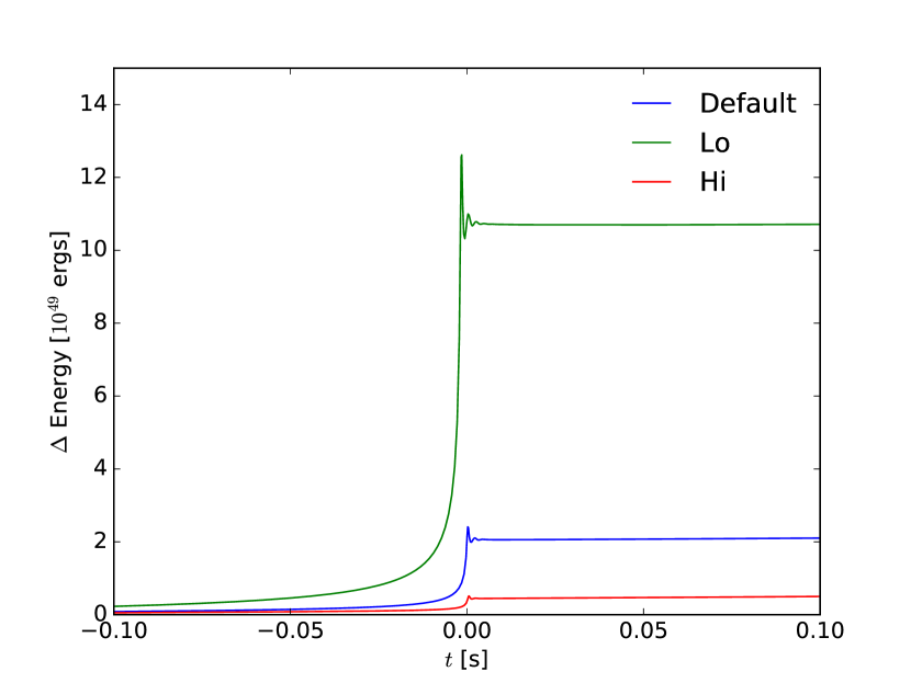
Refer to caption
Figure 20.— The change in total mechanical energy (in 1049superscript104910^{49} erg), defined as the sum of gravitational potential, internal, and kinetic energies, as a function of time after bounce (in seconds) for three different resolutions: Lo (green, 304 radial cells), Default (blue, 608 radial cells), and Hi (red, 1216 radial cells). Energy is conserved to better than 2×10492superscript10492\times 10^{49} erg at bounce for the default resolution, and 3×1048similar-toabsent3superscript1048{\sim}3\times 10^{48} erg at the higher resolution. See text for a discussion.

We perform several spherical 1-d core-collapse hydrodynamical simulations without transport or general-relativistic corrections and with Newtonian gravity to study energy conservation in Fornax. For this test, we use the SFHo equation of state (Steiner et al. 2013). The total mechanical energy is defined as the sum of the kinetic, internal, and gravitational potential energies on the grid, extending out to 20,000 km20000 km20,000\text{ km}. The latter is calculated as:

Egrav=18πG|Φ|2d3x,subscript𝐸grav18𝜋𝐺superscriptΦ2superscript𝑑3𝑥E_{\mathrm{grav}}=-\frac{1}{8\pi G}\int|\nabla\Phi|^{2}d^{3}x\,, (58)

where ΦΦ\Phi is the gravitational potential. We take the jump in total energy around bounce as an apt measure, since gravitation is not implemented in automatically conservative form (the other terms are) and bounce is the most problematic phase of core-collapse simulations vis-à-vis total energy conservation. Moreover, we continue the calculations to 100 mssimilar-toabsent100 ms{\sim}100\text{ ms} after bounce for three resolutions: Lo (304 radial cells, green), Default (608 radial cells, blue), and Hi (1216 radial cells, red). We find that energy is conserved from just before bounce to just after bounce to approximately 1050 erg, 2×1049 erg2superscript1049 erg2\times 10^{49}\text{ erg}, and 3×1048 ergsimilar-toabsent3superscript1048 erg{\sim}3\times 10^{48}\text{ erg}, respectively, for the three resolutions (Figure 20).

Earlier generations of codes, including AGILE-BOLTZTRAN (Liebendörfer et al. 2004) and BETHE-hydro (Murphy & Burrows 2008b), saw total energy shifts from just before bounce to over 100 milliseconds after bounce of on the order of 1051 erg. For comparison, CHIMERA (Bruenn et al., 2009; Bruenn et al., 2016) conserves energy to 0.5 Bethe (1 B=1051 erg1 Bsuperscript1051 erg1\text{ B}=10^{51}\text{ erg}) over 1 ssimilar-toabsent1 s{\sim}1\text{ s} post-bounce. Our default resolution from before bounce to 1 ssimilar-toabsent1 s{\sim}1\text{ s} after bounce conserves total energy to 0.05 B0.05 B0.05\text{ B}, an order of magnitude better. Importantly, we find that the total energy is conserved to 1047 ergsimilar-toabsentsuperscript1047 erg{\sim}10^{47}\text{ erg} from 10 ms10 ms10\text{ ms} post-bounce to 100 ms100 ms100\text{ ms} post-bounce. By comparison, using CoCoNUT for a Newtonian core-collapse simulation, and subtracting out neutrino losses, Müller et al. (2010) report energy conservation of 2×1049 ergsimilar-toabsent2superscript1049 erg{\sim}2\times 10^{49}\text{ erg} from just before bounce to just after bounce, and subsequent non-conservation for the following tens of milliseconds at the 1048similar-toabsentsuperscript1048{\sim}10^{48} level. In §9.1 we perform an analogous core-collapse test using multi-dimensional, multi-species transport.

9. Radiation Tests

9.1. Multi-dimensional Core-collapse Total Energy Conservation Test
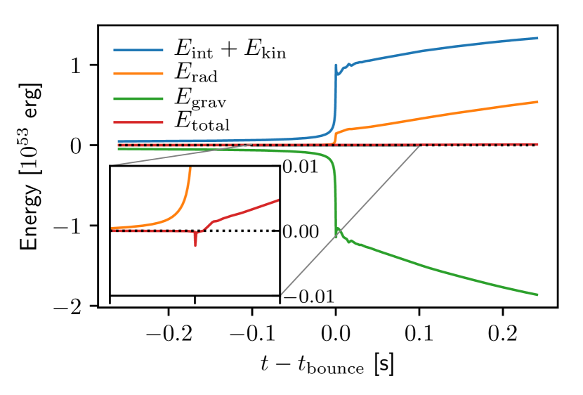
Refer to caption
Figure 21.— We plot the gravitational potential (green), internal and kinetic (blue), and lab-frame radiation (orange) energies (in 1053 erg), as well as the total energy (red) defined as their sum, versus time after bounce (in seconds) for a 2-d, multi-species core-collapse simulation at our default resolution (608 radial cells by 128 polar-angle cells). In this run, we use the 16-Msubscript𝑀direct-productM_{\odot} progenitor model of Woosley & Heger (2007) (which was studied in Vartanyan et al. (2018)) with Newtonian gravity and our dendritic grid decomposed over 1024 processors. At each step of the calculation, we account for the flux of each energy component onto and off of the grid through the outer radial boundary. The inset zooms in on the total energy 100 ms before and after bounce. The total energy is conserved to within a few ×\times1051 ergsimilar-toabsentsuperscript1051 erg{\sim}10^{51}\text{ erg} (to within 0.5% relative to Egravsubscript𝐸gravE_{\mathrm{grav}}) during the entire 500 ms of the run.

As a first test of our full radiation-hydrodynamics code, we test the conservation of total energy by performing a 2-d core-collapse calculation on a grid with a resolution of 608 radial cells by 128 polar-angle cells. We use Newtonian monopolar gravity, the SFHo equation of state, 12 energy groups per species, and our dendritic grid decomposed over 1024 processors. We track the gravitational potential energy (defined as in Eq. 58), internal plus kinetic energy, and the total lab-frame radiation energy at each time step, accounting for the flux of each energy component through the outer radial boundary.

The results of this test are shown in Figure 21. As previously demonstrated in §8.9, we experience a glitch in the total energy at bounce, since gravity is treated in non-conservation form. With radiation transport, there are other additional sources of energy non-conservation, e.g., due to the finite tolerance of the implicit solver or due to truncation of the comoving-to-lab frame transformation in powers of v/c𝑣𝑐v/c. However, as Figure 21 demsontrates, the total energy remains well controlled to within a few×\times1050 ergsimilar-toabsentsuperscript1050 erg{\sim}10^{50}\text{ erg} (or to within 0.5% relative to Egravsubscript𝐸gravE_{\mathrm{grav}}) throughout the 500 ms500 ms500\text{ ms} of the simulation run.777At the same time, the total mass is conserved to within a relative error of 2×10⁸similar-toabsent2superscript108{\sim}2\times 10^{-8}. Energy conservation within such low levels is especially important considering the high-velocity energy fluxes crossing the internal refinement boundaries of our dendritic grid in both the radial and angular directions and across a distribution of many processors.

9.2. Doppler Shift Test

To test the advection of radiation energy in frequency space caused by strong spatial variations in the gas velocity, we perform the Doppler shift test of Vaytet et al. (2011). We use a one-dimensional domain with 50 equally-spaced zones between x=0 cm𝑥0 cmx=0\text{ cm} and x=10 cm𝑥10 cmx=10\text{ cm} with constant background density of ρ=1 g cm3𝜌1superscript g cm3\rho=1\text{ g cm}^{-3} and zero opacity. The velocity varies smoothly between v=0 cm s1𝑣0superscript cm s1v=0\text{ cm s}^{-1} at the left edge of the domain and v=A𝑣𝐴v=A in the center, where A=5×107 cm s1𝐴5superscript107superscript cm s1A=5\times 10^{7}\text{ cm s}^{-1}. At the left boundary, we introduce a radiation field having a Planck spectrum at a temperature T=1000 K𝑇1000 KT=1000\text{ K}, which we resolve using 20 equally-spaced frequency groups from ν=0 Hz𝜈0 Hz\nu=0\text{ Hz} to ν=2×10¹⁴ Hz𝜈2superscript1014 Hz\nu=2\times 10^{14}\text{ Hz}, with two additional groups to account for radiation in the frequency range 2×10¹⁴ Hz2superscript1014 Hz2\times 10^{14}\text{ Hz}\to\infty. We evolve the system for 10 light-crossing times in order to reach a steady state.
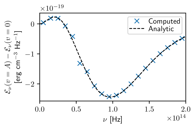
Refer to caption
Figure 22.— Difference between the shifted and unshifted energy spectra for the Doppler shift test. The energy difference in the computed solution (blue exes) and the analytic solution (black dashed line) are plotted. The relative error in the solution is less than 6.5%percent6.56.5\% except near the spectral peak at 5×10¹³ Hzsimilar-toabsent5superscript1013 Hz\sim 5\times 10^{13}\text{ Hz} where it jumps up to 23%percent2323\% due to slope limiting of the frequency-advected spectrum, which results in a local first-order error.

In Figure 22, we plot the difference between the Doppler-shifted spectral energy distribution at the center of the domain, ν(v=A)subscript𝜈𝑣𝐴\mathcal{E}_{\nu}(v=A), and the unshifted distribution at the left boundary, ν(v=0)subscript𝜈𝑣0\mathcal{E}_{\nu}(v=0). We also plot the analytic solution, obtained from the difference between the relativistic Doppler shift of the incident spectrum into the frame comoving at velocity v=A𝑣𝐴v=A and the unshifted spectrum. To do this, we first multiply the lab-frame frequencies by the relativistic Doppler factor,

1+β1β,1𝛽1𝛽\sqrt{\frac{1+\beta}{1-\beta}}\,, (59)

where β=A/c𝛽𝐴𝑐\beta=A/c, to obtain the corresponding comoving-frame frequencies. Then, we set ν=(4π/c)Bνsubscript𝜈4𝜋𝑐subscript𝐵𝜈\mathcal{E}_{\nu}=(4\pi/c)B_{\nu}, with frequencies evaluated in the comoving frame, and finally divide by the relativistic Doppler factor to transform the resulting spectrum back into the laboratory frame.

The computed solution agrees well with the analytic solution at almost all frequencies. The relative error is slightly larger near ν5×10¹³ Hzsimilar-to𝜈5superscript1013 Hz\nu\sim 5\times 10^{13}\text{ Hz}, the peak of the Planck spectrum at T=1000 K𝑇1000 KT=1000\text{ K}, where TVD slope limiting in our frequency advection step results in a local first-order error. With 20 groups, the relative error is less than 6.5%similar-toabsentpercent6.5\sim 6.5\% away from the spectral peak, where it jumps up to 23%similar-toabsentpercent23\sim 23\%. Running the same test with 40 groups reduces the maximum relative error to 0.85%percent0.850.85\% away from the spectral peak, where it jumps to 5.6%percent5.65.6\%.

9.2.1 Continuity of Lab-Frame Flux at Transparent Shocks
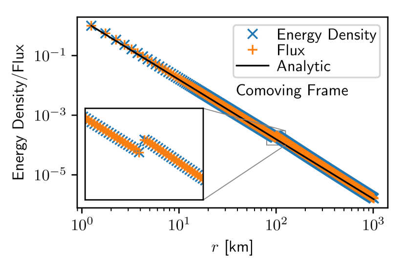
Refer to caption
Refer to caption
Figure 23.— Left: The profiles of the radiation energy density and flux, scaled to their values in the first radial zone, in the comoving frame versus radius for a steady-state constant point luminosity source. A non-trivial radial velocity field has been imposed that includes a strong standing shock (see Eq. 60). Right: The corresponding scaled radiation energy density and flux profiles Lorentz-transformed into the laboratory frame. We note that the matter is assumed to be transparent, hence the laboratory-frame profiles of the scaled radiation quantities should go as 1/r21superscript𝑟21/r^{2}, which we indicate by the solid line. See text for a discussion.

To demonstrate further that Fornax accounts properly for frame effects, we show a comparison of the radial profile of the total radiation energy density and flux calculated in the steady state for a constant point luminosity source at the spherical grid center. We set the material opacity to zero and impose a core-collapse-like radial velocity field given by

v(r)={0.1vshockrrshock,r<rshockvshockrmax/r1rmax/rshock1,rrshock,𝑣𝑟cases0.1subscript𝑣shock𝑟subscript𝑟shock𝑟subscript𝑟shocksubscript𝑣shocksubscript𝑟max𝑟1subscript𝑟maxsubscript𝑟shock1𝑟subscript𝑟shockv(r)=\left\{\begin{array}[]{ll}-0.1\,v_{\mathrm{shock}}\frac{r}{r_{\mathrm{shock}}},&r<r_{\mathrm{shock}}\\ -v_{\mathrm{shock}}\frac{\sqrt{r_{\mathrm{max}}/r}-1}{\sqrt{r_{\mathrm{max}}/r_{\mathrm{shock}}}-1},&r\geq r_{\mathrm{shock}}\end{array}\right., (60)

where rshock=100 kmsubscript𝑟shock100 kmr_{\mathrm{shock}}=100\text{ km} is the location of a strong standing shock of maximum velocity vshock=0.1csubscript𝑣shock0.1𝑐v_{\mathrm{shock}}=0.1c and rmax=1000 kmsubscript𝑟max1000 kmr_{\mathrm{max}}=1000\text{ km} is the maximum radius.

Since Fornax calculates radiation quantities in the comoving frame, the corresponding energy density and flux profiles will have discontinuities at shocks. However, since the radiation is uncoupled from the matter, the radiation quantities should possess a smooth profile that goes as 1/r21superscript𝑟21/r^{2} in the laboratory frame. Thus, performing a simple Lorentz transformation back to the laboratory frame should eliminate the discontinuity. Figure 23 depicts the radial profiles of the radiation energy density and flux, each scaled to their values in the first radial zone, with the left and right panels depicting the profile in the comoving and laboratory frames, respectively. The right-hand-side panel shows that the Lorentz transformation has indeed removed the discontinuity. This simple test is one way of demonstrating that Fornax handles the velocity-dependent terms in radiation Equations (3a) and (3b) properly.

9.3. Frequency-Dependent Opacity Test

To test the effect of a strong velocity gradient on a frequency-dependent opacity function, we perform a modified version of a test by Vaytet et al. (2011). We use a one-dimensional domain with x[0,1] cm𝑥01 cmx\in[0,1]\text{ cm} resolved over 100 zones and set a fixed velocity profile v=𝒟x𝑣𝒟𝑥v=\mathcal{D}x, where 𝒟𝒟\mathcal{D} is either 0 s10superscript s10\text{ s}^{-1} or 107 s1superscript107superscript s110^{7}\text{ s}^{-1}. We use a density profile of ρ=1/(𝒞x)𝜌1𝒞𝑥\rho=1/(\mathcal{C}x) with 𝒞=0.2 cm2 g1𝒞0.2superscript cm2superscript g1\mathcal{C}=0.2\text{ cm}^{2}\text{ g}^{-1} and set the gas temperature to T0=3 Ksubscript𝑇03 KT_{0}=3\text{ K} everywhere. We use a frequency-dependent opacity with κν=100 cm2 g1subscript𝜅𝜈100superscript cm2superscript g1\kappa_{\nu}=100\text{ cm}^{2}\text{ g}^{-1} for ν<2×10¹³ Hz𝜈2superscript1013 Hz\nu<2\times 10^{13}\text{ Hz}, transitioning smoothly to κν=1 cm2 g1subscript𝜅𝜈1superscript cm2superscript g1\kappa_{\nu}=1\text{ cm}^{2}\text{ g}^{-1} over a region of width Δν=4.5×10⁹ HzΔ𝜈4.5superscript109 Hz\Delta\nu=4.5\times 10^{9}\text{ Hz} as shown in Figure 24. At the left boundary, we inject a Gaussian radiation spectrum that is normalized to have total energy aRT14subscript𝑎Rsuperscriptsubscript𝑇14a_{\mathrm{R}}T_{1}^{4} with T1=1000 Ksubscript𝑇11000 KT_{1}=1000\text{ K}, is peaked at ν=2×10¹³ Hz𝜈2superscript1013 Hz\nu=2\times 10^{13}\text{ Hz}, has FWHM equal to two-thirds the width of the transition region, and is resolved over 20 equally-spaced frequency groups (also shown in Figure 24). For each case, we evolve only the radiation system for one light crossing time, keeping the hydrodynamics frozen.
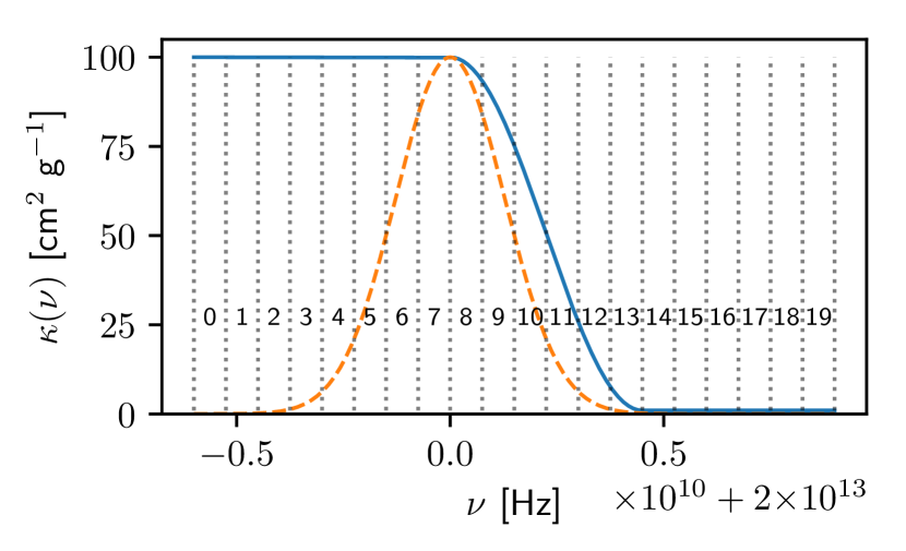
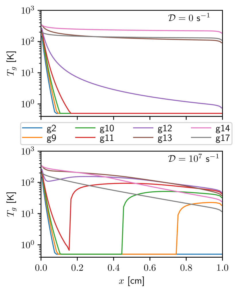
Refer to caption
Figure 24.— Opacity function (solid blue line) for the frequency-dependent opacity test. The opacity changes from κν=100 cm2 g1subscript𝜅𝜈100superscript cm2superscript g1\kappa_{\nu}=100\text{ cm}^{2}\text{ g}^{-1} for ν<2×10¹³ Hz𝜈2superscript1013 Hz\nu<2\times 10^{13}\text{ Hz} to κν=1 cm2 g1subscript𝜅𝜈1superscript cm2superscript g1\kappa_{\nu}=1\text{ cm}^{2}\text{ g}^{-1}, transitioning smoothly over a frequency range of width Δν=4.5×10⁹ HzΔ𝜈4.5superscript109 Hz\Delta\nu=4.5\times 10^{9}\text{ Hz}. Overplotted is a scaled representation of the incident energy spectrum (dashed orange line), which peaks at ν=2×10¹³ Hz𝜈2superscript1013 Hz\nu=2\times 10^{13}\text{ Hz} and has FWHM equal to 2/3Δν23Δ𝜈2/3\Delta\nu. The numbered frequency groups are indicated by vertical dotted lines. Groups 8-13 comprise the opacity transition region.
Refer to caption
Figure 25.— Selected group temperatures, Tg(g/aR)1/4subscript𝑇𝑔superscriptsubscript𝑔subscript𝑎R14T_{g}\equiv(\mathcal{E}_{g}/a_{\mathrm{R}})^{1/4} for the frequency-dependent opacity test. The velocity profile is given by v=𝒟x𝑣𝒟𝑥v=\mathcal{D}x, where either 𝒟=0 s1𝒟0superscript s1\mathcal{D}=0\text{ s}^{-1} for the zero-gradient case (top) or 𝒟=107 s1𝒟superscript107superscript s1\mathcal{D}=10^{7}\text{ s}^{-1} for the strong velocity gradient case (bottom). For the zero-velocity case, only radiation in groups with very low opacities can stream freely across the domain, but for the case with a strong velocity gradient, energy in groups 9-12 inside the opacity transition region are shifted to higher frequencies where the opacities are smaller. This allows these groups to stream more freely once optically thin conditions are reached.

Figure 25 shows selected group temperatures, Tg(g/aR)1/4subscript𝑇𝑔superscriptsubscript𝑔subscript𝑎R14T_{g}\equiv(\mathcal{E}_{g}/a_{\mathrm{R}})^{1/4}, for the cases with 𝒟=0 s1𝒟0superscript s1\mathcal{D}=0\text{ s}^{-1} (top) and 𝒟=107 s1𝒟superscript107superscript s1\mathcal{D}=10^{7}\text{ s}^{-1} (bottom). In the zero-velocity case, the group energies are unshifted, and only those groups with low enough optical depth are able to stream freely across the domain. By contrast, in the case with a strong velocity gradient, the comoving-frame frequencies are Doppler-shifted to the right where the opacities are lower. Thus, the energy in groups 9-12 in the transition region of the opacity function are able to stream more freely once optically-thin conditions are reached.

9.4. Multi-Group Radiation Pulse Advection

To study the behavior of Fornax in the strong diffusion regime, where radiation is transported both by diffusion through the gas and advection along with it, we perform a variation of the pulse advection test of Krumholz et al. (2007) (see also Zhang et al. 2013), modified for our explicit transport solver. We initialize the gas temperature and density profiles as

T𝑇\displaystyle T =\displaystyle= T0+(T1T0)exp(x22w2),subscript𝑇0subscript𝑇1subscript𝑇0superscript𝑥22superscript𝑤2\displaystyle T_{0}+(T_{1}-T_{0})\exp\left(-\frac{x^{2}}{2w^{2}}\right), (61)
ρ𝜌\displaystyle\rho =\displaystyle= ρ0T0T1+aRμ3kB(T04TT3),subscript𝜌0subscript𝑇0subscript𝑇1subscript𝑎R𝜇3subscript𝑘Bsuperscriptsubscript𝑇04𝑇superscript𝑇3\displaystyle\rho_{0}\frac{T_{0}}{T_{1}}+\frac{a_{\mathrm{R}}\mu}{3k_{\mathrm{B}}}\left(\frac{T_{0}^{4}}{T}-T^{3}\right), (62)

where T0subscript𝑇0T_{0} and ρ0subscript𝜌0\rho_{0} are the background temperature and density, respectively, T1=2T0subscript𝑇12subscript𝑇0T_{1}=2T_{0} is the peak of a Gaussian pulse of thermal energy of width w𝑤w, and μ=(me+mp)/2𝜇subscript𝑚𝑒subscript𝑚𝑝2\mu=(m_{e}+m_{p})/2 is the mean particle mass for ionized hydrogen. Following Zhang et al. (2013), we use a temperature- and frequency-dependent absorption opacity of the form

κν(T)=κ0(TT1)1/2(νν1)3[1exp(hνkBT)],subscript𝜅𝜈𝑇subscript𝜅0superscript𝑇subscript𝑇112superscript𝜈subscript𝜈13delimited-[]1𝜈subscript𝑘B𝑇\kappa_{\nu}(T)=\kappa_{0}\left(\frac{T}{T_{1}}\right)^{-1/2}\left(\frac{\nu}{\nu_{1}}\right)^{-3}\left[1-\exp\left(-\frac{h\nu}{k_{\mathrm{B}}T}\right)\right]\,, (63)

where κ0subscript𝜅0\kappa_{0} is some normalization constant and we take ν1=2.821kBT1/hsubscript𝜈12.821subscript𝑘Bsubscript𝑇1\nu_{1}=2.821k_{\mathrm{B}}T_{1}/h to approximate the spectral peak of a Planck distribution at temperature T1subscript𝑇1T_{1}. The problem dimensions are set by the choice of an arbitrary length scale, w𝑤w, and by the values of the non-dimensional parameters βv/c𝛽𝑣𝑐\beta\equiv v/c, v/a0𝑣subscript𝑎0\mathcal{M}\equiv v/a_{0}, 𝒫aRT04/(ρ0a02)𝒫subscript𝑎Rsuperscriptsubscript𝑇04subscript𝜌0superscriptsubscript𝑎02\mathcal{P}\equiv a_{\mathrm{R}}T_{0}^{4}/(\rho_{0}a_{0}^{2}), and τκP(T1)w𝜏subscript𝜅Psubscript𝑇1𝑤\tau\equiv\kappa_{\mathrm{P}}(T_{1})w, where κP=3.457κ0(T/T1)3.5subscript𝜅P3.457subscript𝜅0superscript𝑇subscript𝑇13.5\kappa_{\mathrm{P}}=3.457\,\kappa_{0}(T/T_{1})^{-3.5} is the Planck-mean opacity such that τ𝜏\tau represents the optical depth of the pulse. For our version of this problem, we choose w=1 cm𝑤1 cmw=1\text{ cm}, β=0.01𝛽0.01\beta=0.01, =0.10.1\mathcal{M}=0.1, 𝒫=0.1𝒫0.1\mathcal{P}=0.1, and κ0=0.2892τ cm1subscript𝜅00.2892𝜏superscript cm1\kappa_{0}=0.2892\,\tau\text{ cm}^{-1}, where τ𝜏\tau is chosen to control which diffusion regime characterizes the flow.

The product βτ𝛽𝜏\beta\tau is equal to the ratio of the radiation diffusion and advection time scales. For βτ1less-than-or-similar-to𝛽𝜏1\beta\tau\lesssim 1, radiation diffusion dominates and the system is in the so-called “static diffusion” regime, but for βτ1much-greater-than𝛽𝜏1\beta\tau\gg 1, advection dominates and the system is in the “dynamic diffusion” regime. In either case, although the velocity-dependent radiation work and advection terms will be very different depending on the frame in which the equations are solved, the results should be frame-independent. Therefore, for both the static and dynamic diffusion regimes, we compare runs in which the radiation pulse is initially at rest to runs in which the radiation pulse is advected over twice its initial width and shifted back to lie on top of the unadvected results. In either case, with τ1much-greater-than𝜏1\tau\gg 1, the radiation is in thermal equilibrium with the gas, and the total pressure is initially constant.
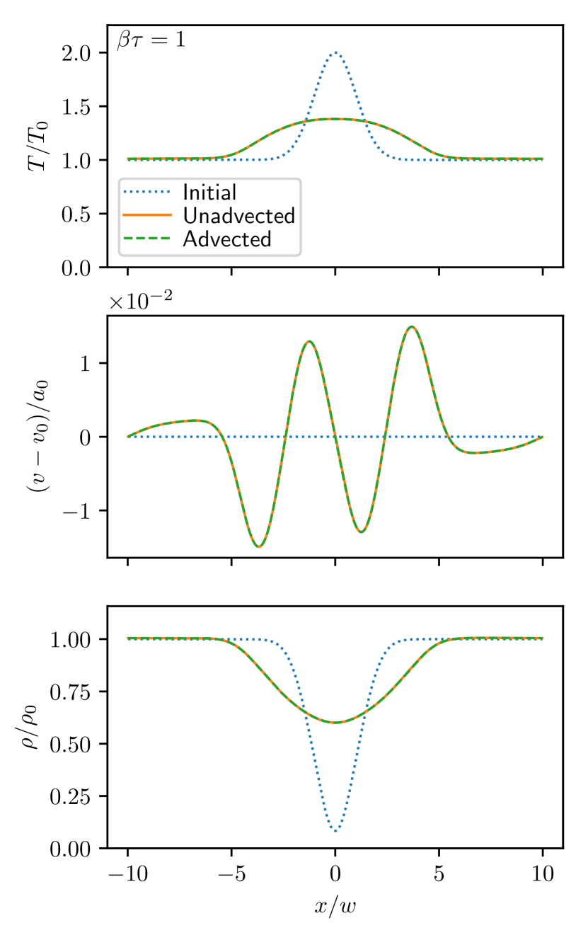
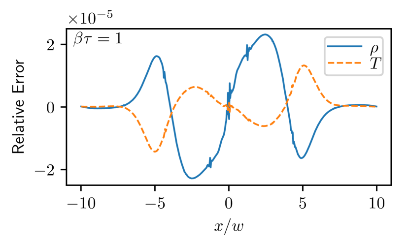
Refer to caption
Figure 26.— Temperature (top), velocity (middle), and density (bottom) for the multigroup pulse advection test with βτ=1𝛽𝜏1\beta\tau=1 in the static diffusion regime. Profiles at the initial time (dotted blue line) and at time t=2w/βc𝑡2𝑤𝛽𝑐t=2w/\beta c for the unadvected (solid orange line) and advected (dashed green line) runs are shown. In both runs, the radiation pulse diffuses through the gas, and as pressure support is lost, the density in the pulse increases. Although the radiative work and advection terms are very different between the unadvected and advected runs, the relative error between them is so small that they are visually indistinguishable (see Figure 27 for a plot of the errors).
Refer to caption
Figure 27.— Relative errors between the unadvected and advected runs for the density (solid blue line) and temperature (dashed orange line) in the multigroup pulse advection test in the static diffusion regime with βτ=1𝛽𝜏1\beta\tau=1 (see Figure 26 for their profiles). The relative errors are bounded in absolute value by 2.3×1052.3superscript1052.3\times 10^{-5} and 1.4×1051.4superscript1051.4\times 10^{-5} for the density and temperature, respectively. This indicates very good agreement between these runs, despite the fact that the radiative work and advection terms are very different from the vantage of the different frames.

We use a computational grid of length L=20w𝐿20𝑤L=20w resolved over 512512512 zones, with 888 radiation groups logarithmically-spaced over the frequency range [4×1018,4×1022] Hz4superscript10184superscript1022 Hz[4\times 10^{18},4\times 10^{22}]\text{ Hz}. In Figure 26, we show the resulting temperature, velocity, and density profiles for both the advected and unadvected runs with τ=100𝜏100\tau=100 such that βτ=1𝛽𝜏1\beta\tau=1, putting the system is in the static diffusion regime. Over the course of the run, the radiation has diffused through the gas, decreasing the temperature and thermal pressure support in the pulse, hence the density increases correspondingly. Since the advected and unadvected runs are visually indistinguishable, we plot the relative errors of the density and temperature in Figure 27, which are bounded by 2.3×1052.3superscript1052.3\times 10^{-5} and 1.4×1051.4superscript1051.4\times 10^{-5}, respectively, in absolute value.

Refer to caption
Figure 28.— Same as Figure 26 but for βτ=100𝛽𝜏100\beta\tau=100 in the dynamic diffusion regime. Here, the radiation is trapped within the pulse and there is hardly any diffusion as it is advected across the grid. Again, the profiles for the unadvected (solid orange line) and advected (dashed green line) runs are visually indistinguishable (see Figure 29 for their relative errors).
Refer to caption
Figure 29.— Same as Figure 27 but in the dynamic diffusion regime with βτ=100𝛽𝜏100\beta\tau=100. The relative errors are bounded in absolute value by 1.4×1031.4superscript1031.4\times 10^{-3} and 1.5×1041.5superscript1041.5\times 10^{-4} for the density and temperature, respectively. Again, this demonstrates good agreement between the unadvected and advected runs, although the relative sizes of the terms is very different in each frame.

Similarly, in Figure 28, we plot the results for the case with τ=104𝜏superscript104\tau=10^{4} such that βτ=100𝛽𝜏100\beta\tau=100, which puts the system in the dynamic diffusion regime. This time, there is hardly any diffusion as the pulse is advected, since the radiation is effectively trapped within the gas. In Figure 29, we plot the relative errors of the density and temperature, which are bounded by 1.4×1031.4superscript1031.4\times 10^{-3} and 1.5×1041.5superscript1041.5\times 10^{-4}, respectively, in absolute value.

Importantly, these results demonstrate the ability of Fornax to reproduce the correct behavior to a high degree of accuracy in both the static and dynamic diffusion regimes and for both advected and unadvected flows. This represents a very sensitive test of the code’s ability to model radiative trapping in the CCSN. In the core-collapse supernova context, trapping of νesubscript𝜈𝑒\nu_{e}s by infalling matter and their subsequent compression produces a spectrum of degenerate νesubscript𝜈𝑒\nu_{e}s whose energies can reach the 100300 MeVsimilar-toabsent100300 MeV\sim 100-300\text{ MeV} range while preserving a relatively high lepton fraction, which is a critically important aspect that allows the core to reach nuclear densities at bounce.

9.5. Multi-group Gray-Opacity Non-Equilibrium Radiation Shock

To test the Fornax code’s ability to couple the multigroup radiation subsystem to the hydrodynamics in a regime where the fluid and radiation are out of equilibrium, we present here the results of the classical gray non-equilibrium radiation shock described by Zel’Dovich & Raizer (1969). Following that work, we adopt the Eddington approximation and set the radiation pressure tensor to (𝒫ϵ)ji=(ϵ/3)δjisubscriptsuperscriptsubscript𝒫italic-ϵ𝑖𝑗subscriptitalic-ϵ3subscriptsuperscript𝛿𝑖𝑗(\mathcal{P}_{\epsilon})^{i}_{j}=(\mathcal{E}_{\epsilon}/3)\delta^{i}_{j}, where δjisubscriptsuperscript𝛿𝑖𝑗\delta^{i}_{j} is the Kronecker symbol. The shock structure has a semi-analytic solution described by Lowrie & Edwards (2008). Using their parameters with an upstream Mach number of =33\mathcal{M}=3, we obtain a subcritical radiation shock whose temperature jumps discontinuously at the shock interface. We set the constant, gray absorption opacity to κ=577 cm1𝜅577superscript cm1\kappa=577\text{ cm}^{-1}, the mean particle mass to μ=mH𝜇subscript𝑚H\mu=m_{\mathrm{H}}, and use an adiabatic EOS with γ=5/3𝛾53\gamma=5/3. We use a one-dimensional Cartesian domain with x[0.0132, 0.00255]𝑥0.01320.00255x\in[-0.0132,\,0.00255] resolved over Nx=512subscript𝑁𝑥512N_{x}=512 zones. The problem is set in the rest frame of the shock, which we initialize at x=0𝑥0x=0. In the upstream state (x<0𝑥0x<0), we set the gas temperature T0=2.18×10⁶ Ksubscript𝑇02.18superscript106 KT_{0}=2.18\times 10^{6}\text{ K}, density ρ0=5.69 g cm3subscript𝜌05.69superscript g cm3\rho_{0}=5.69\text{ g cm}^{-3}, and velocity v0=5.19×107 cm s1subscript𝑣05.19superscript107superscript cm s1v_{0}=5.19\times 10^{7}\text{ cm s}^{-1}, and using the Rankine-Hugoniot jump conditions to determine the downstream state (x<0𝑥0x<0), we set T1=7.98×10⁶ Ksubscript𝑇17.98superscript106 KT_{1}=7.98\times 10^{6}\text{ K}, density ρ1=17.1 g cm3subscript𝜌117.1superscript g cm3\rho_{1}=17.1\text{ g cm}^{-3}, and velocity v1=1.73×107 cm s1subscript𝑣11.73superscript107superscript cm s1v_{1}=1.73\times 10^{7}\text{ cm s}^{-1}. Similar to Vaytet et al. (2011), we use 8 radiation groups logarithmically spaced over the frequency range ν[1015 Hz, 1019 Hz]𝜈superscript1015 Hzsuperscript1019 Hz\nu\in[10^{15}\text{ Hz},\,10^{19}\text{ Hz}], initialize the group radiation energy densities using a Planck spectrum at the local gas temperature with zero radiation flux, and evolve for 3 shock-crossing times to tfinal=9.08×10¹⁰ ssubscript𝑡final9.08superscript1010 st_{\mathrm{final}}=9.08\times 10^{-10}\text{ s}. Finally, since the structure of the steady-state shock solution is independent of the radiation propagation speed, c^^𝑐\hat{c}, and since we must solve the semi-explicit radiation subsystem on a hydrodynamic time scale, we adopt a reduced speed of light c^=10(v0+a0)^𝑐10subscript𝑣0subscript𝑎0\hat{c}=10(v_{0}+a_{0}), where a0=1.73×107 cm s1subscript𝑎01.73superscript107superscript cm s1a_{0}=1.73\times 10^{7}\text{ cm s}^{-1} is the upstream sound speed.

Refer to caption
Figure 30.— Computed gas temperature (blue points) and radiation temperature (orange points) for the multigroup gray radiation shock with their semi-analytic solutions (black lines) overplotted and an inset showing the detail of the non-equilibrium Zel’Dovich spike region.

Figure 30 shows the gas temperature structure at time tfinalsubscript𝑡finalt_{\mathrm{final}} with the semi-analytic solution from Lowrie & Edwards (2008) overplotted and an inset showing the detail of the Zel’Dovich spike in the upstream temperature near the shock interface. There is very good agreement between the two solutions, including in the non-equilibrium spike region and in the radiatively-heated shock precursor in the downstream state. The relative error between the solutions is bounded by 0.8% everywhere; the agreement in the remaining variables is similarly good. Since this test simultaneously exercises the multi-group, velocity-dependent, Doppler-shift, and matter-radiation coupling features of the Fornax code, it also simultaneously demonstrates the code’s ability to compute the most problematic aspects of full radiation-hydrodynamics accurately and consistently.

10. Conclusion

In this paper, we have described the methods and implementation of the multi-group, multi-dimensional, radiation-hydrodynamic code Fornax and numerically exercised it with a variety of standard and non-standard simulation tests. These included tests of on- and off-center Sedov blast waves, the Sod shock tube, double Mach reflection, the 2-d and 3-d Rayleigh-Taylor and 2-d Kelvin-Helmholtz instabilities, the Liska-Wendroff implosion, pressureless dust collapse, energy conservation with gravity and a complicated EOS, radiation advection and Doppler (v/c𝑣𝑐v/c) shifts in the context of strong velocity gradients, the handling of velocity- and frequency-dependent opacity, and non-equilibirum radiative shocks with the Zel’Dovich spike. We demonstrated that Fornax performs well and accurately for all these tests, robustly handling non-trivial multi-dimensional hydrodynamic and radiation-hydrodynamic problems. To date, Fornax has been employed to study core-collapse supernovae (Wallace et al. 2016; Radice et al. 2017; Burrows et al. 2018; Vartanyan et al. 2018; Seadrow et al. 2018), for which extensions that include approximate general relativity and inelastic scattering processes are of relevance. The implementation of these effects is not address here, but can be found in Marek et al. (2006) (for the former) and Thompson, Burrows, & Pinto (2003) and Burrows & Thompson (2004) (for the latter). In constructing Fornax, we endeavored to incorporate best numerical and solution practices, with the result that the code is fast, scales well on most modern HPC platforms, and has useful geometrical and grid flexibilities. Given this, we anticipate its continued use to explore cutting-edge radiation-hydrodynamical challenges of astrophysical import and plan to extend its reach to include magnetic fields and neutrino oscillations in the years to come.

The authors acknowledge support under U.S. NSF Grant AST-1714267, the Max-Planck/Princeton Center (MPPC) for Plasma Physics (NSF PHY-1144374), and the U.S. Department of Energy, Office of Science, Office of Advanced Scientific Computing Research, and the Scientific Discovery through Advanced Computing (SciDAC4) program under Grant DE-SC0018297 (subaward 00009650). DR acknowledges support as a Frank and Peggy Taplin Fellow at the Institute for Advanced Study. The authors employed computational resources provided by the TIGRESS high performance computer center at Princeton University, which is jointly supported by the Princeton Institute for Computational Science and Engineering (PICSciE) and the Princeton University Office of Information Technology, and by the National Energy Research Scientific Computing Center (NERSC), which is supported by the Office of Science of the US Department of Energy (DOE) under contract DE-AC03-76SF00098. The authors express their gratitude to Ted Barnes of the DOE Office of Nuclear Physics for facilitating their use of NERSC. This research is part of the Blue Waters sustained-petascale computing project, which is supported by the National Science Foundation (awards OCI-0725070 and ACI-1238993) and the state of Illinois. This work is also part of the “Three-Dimensional Simulations of Core-Collapse Supernovae” PRAC allocation support by the National Science Foundation (under award #OAC-1809073). Blue Waters is a joint effort of the University of Illinois at Urbana-Champaign and its National Center for Supercomputing Applications. Under the local award #TG-AST170045, this work used the resource Stampede2 in the Extreme Science and Engineering Discovery Environment (XSEDE), which is supported by National Science Foundation grant number ACI-1548562. This work was performed under the auspices of the U.S. Department of Energy by Lawrence Livermore National Laboratory under Contract DE-AC52-07NA27344. This article has been assigned an LLNL document release number LLNL-JRNL-752999-DRAFT. In additoon, this work was performed in the auspices of the U.S. Department of Energy by Los Alamos National Laboratory under Contract DE-AC52-06NA25396. This article has been assigned an LANL document release number LA-UR-18-25082.

Appendix A General Spherical Metric

We use the general spherical coordinates (x1,x2,x3)superscript𝑥1superscript𝑥2superscript𝑥3(x^{1},x^{2},x^{3}), where the physical spherical coordinates are related via the mappings

r(x1)𝑟superscript𝑥1\displaystyle r(x^{1}) =rtsinh(|x1|rt),absentsubscript𝑟𝑡superscript𝑥1subscript𝑟𝑡\displaystyle=r_{t}\sinh\left(\frac{|x^{1}|}{r_{t}}\right)\,, (A1a)
θ(x2)𝜃superscript𝑥2\displaystyle\theta(x^{2}) =π2+Cx2[1+11+α(x2xt)α],absent𝜋2𝐶superscript𝑥2delimited-[]111𝛼superscriptsuperscript𝑥2subscript𝑥𝑡𝛼\displaystyle=\frac{\pi}{2}+Cx^{2}\left[1+\frac{1}{1+\alpha}\left(\frac{x^{2}}{x_{t}}\right)^{\alpha}\right]\,, (A1b)
ϕ(x3)italic-ϕsuperscript𝑥3\displaystyle\phi(x^{3}) =x3.absentsuperscript𝑥3\displaystyle=x^{3}\,. (A1c)

The invariant proper interval for regular spherical coordinates is given by

ds2=dr2+r2dθ2+r2sin2θdϕ2.𝑑superscript𝑠2𝑑superscript𝑟2superscript𝑟2𝑑superscript𝜃2superscript𝑟2superscript2𝜃𝑑superscriptitalic-ϕ2ds^{2}=dr^{2}+r^{2}\,d\theta^{2}+r^{2}\sin^{2}\theta\,d\phi^{2}\,. (A2)

For general spherical coordinates, such as those defined by Equations (A1), the invariant proper interval is given via the Chain Rule by

ds2𝑑superscript𝑠2\displaystyle ds^{2} =(1r)2(dx1)2absentsuperscriptsubscript1𝑟2superscript𝑑superscript𝑥12\displaystyle=(\partial_{1}r)^{2}(dx^{1})^{2}
+r2(2θ)2(dx2)2superscript𝑟2superscriptsubscript2𝜃2superscript𝑑superscript𝑥22\displaystyle+\,r^{2}(\partial_{2}\theta)^{2}(dx^{2})^{2}
+r2sin2θ(dx3)2.superscript𝑟2superscript2𝜃superscript𝑑superscript𝑥32\displaystyle+\,r^{2}\sin^{2}\theta(dx^{3})^{2}\,. (A3)

Thus, with ds2gμνdxμdxν𝑑superscript𝑠2subscript𝑔𝜇𝜈𝑑superscript𝑥𝜇𝑑superscript𝑥𝜈ds^{2}\equiv g_{\mu\nu}\,dx^{\mu}\,dx^{\nu}, we identify the metric components as

g11subscript𝑔11\displaystyle g_{11} =(1r)2,absentsuperscriptsubscript1𝑟2\displaystyle=(\partial_{1}r)^{2}\,, (A4a)
g22subscript𝑔22\displaystyle g_{22} =r2(2θ)2,absentsuperscript𝑟2superscriptsubscript2𝜃2\displaystyle=r^{2}(\partial_{2}\theta)^{2}\,, (A4b)
g33subscript𝑔33\displaystyle g_{33} =r2sin2θ.absentsuperscript𝑟2superscript2𝜃\displaystyle=r^{2}\sin^{2}\theta\,. (A4c)

Since the metric gμνsubscript𝑔𝜇𝜈g_{\mu\nu} is orthogonal (diagonal), the contravariant components are simply the inverses of their covariant counterparts, i.e., gii=(gii)1superscript𝑔𝑖𝑖superscriptsubscript𝑔𝑖𝑖1g^{ii}=(g_{ii})^{-1} for i=1,2,3𝑖123i=1,2,3. The contravariant and covariant components of the metric can be used to raise and lower indices, respectively, i.e.,

vμsuperscript𝑣𝜇\displaystyle v^{\mu} =gμνvν,absentsuperscript𝑔𝜇𝜈subscript𝑣𝜈\displaystyle=g^{\mu\nu}v_{\nu}\,, (A5)
vνsubscript𝑣𝜈\displaystyle v_{\nu} =gμνvμ.absentsubscript𝑔𝜇𝜈superscript𝑣𝜇\displaystyle=g_{\mu\nu}v^{\mu}\,. (A6)

Finally, the determinant of the metric, |g|𝑔|g|, is defined as

|g|=r2(1r)sinθ(2θ).𝑔superscript𝑟2subscript1𝑟𝜃subscript2𝜃\sqrt{|g|}=r^{2}(\partial_{1}r)\sin\theta\,(\partial_{2}\theta)\,. (A7)

Appendix B Covariant Form of the Momentum Equation

In Equation 1b, the covariant derivative of the tensor is defined as

Tν;σμTν,σμ+ΓσλμTνλΓσνλTλμ,subscriptsuperscript𝑇𝜇𝜈𝜎subscriptsuperscript𝑇𝜇𝜈𝜎subscriptsuperscriptΓ𝜇𝜎𝜆subscriptsuperscript𝑇𝜆𝜈subscriptsuperscriptΓ𝜆𝜎𝜈subscriptsuperscript𝑇𝜇𝜆\mathchoice{T^{\leavevmode{\mu}\mathchoice{\makebox[10.56886pt][c]{$\displaystyle$}}{\makebox[10.56886pt][c]{$\textstyle$}}{\makebox[6.58156pt][c]{$\scriptstyle$}}{\makebox[4.70108pt][c]{$\scriptscriptstyle$}}}_{\mathchoice{\makebox[4.21783pt][c]{$\displaystyle$}}{\makebox[4.21783pt][c]{$\textstyle$}}{\makebox[2.95248pt][c]{$\scriptstyle$}}{\makebox[2.10892pt][c]{$\scriptscriptstyle$}}\leavevmode{\nu;\sigma}}}{T^{\leavevmode{\mu}\mathchoice{\makebox[10.56886pt][c]{$\displaystyle$}}{\makebox[10.56886pt][c]{$\textstyle$}}{\makebox[6.58156pt][c]{$\scriptstyle$}}{\makebox[4.70108pt][c]{$\scriptscriptstyle$}}}_{\mathchoice{\makebox[4.21783pt][c]{$\displaystyle$}}{\makebox[4.21783pt][c]{$\textstyle$}}{\makebox[2.95248pt][c]{$\scriptstyle$}}{\makebox[2.10892pt][c]{$\scriptscriptstyle$}}\leavevmode{\nu;\sigma}}}{T^{\leavevmode{\mu}\mathchoice{\makebox[10.56886pt][c]{$\displaystyle$}}{\makebox[10.56886pt][c]{$\textstyle$}}{\makebox[6.58156pt][c]{$\scriptstyle$}}{\makebox[4.70108pt][c]{$\scriptscriptstyle$}}}_{\mathchoice{\makebox[4.21783pt][c]{$\displaystyle$}}{\makebox[4.21783pt][c]{$\textstyle$}}{\makebox[2.95248pt][c]{$\scriptstyle$}}{\makebox[2.10892pt][c]{$\scriptscriptstyle$}}\leavevmode{\nu;\sigma}}}{T^{\leavevmode{\mu}\mathchoice{\makebox[10.56886pt][c]{$\displaystyle$}}{\makebox[10.56886pt][c]{$\textstyle$}}{\makebox[6.58156pt][c]{$\scriptstyle$}}{\makebox[4.70108pt][c]{$\scriptscriptstyle$}}}_{\mathchoice{\makebox[4.21783pt][c]{$\displaystyle$}}{\makebox[4.21783pt][c]{$\textstyle$}}{\makebox[2.95248pt][c]{$\scriptstyle$}}{\makebox[2.10892pt][c]{$\scriptscriptstyle$}}\leavevmode{\nu;\sigma}}}\equiv\mathchoice{T^{\leavevmode{\mu}\mathchoice{\makebox[10.17998pt][c]{$\displaystyle$}}{\makebox[10.17998pt][c]{$\textstyle$}}{\makebox[6.30934pt][c]{$\scriptstyle$}}{\makebox[4.50664pt][c]{$\scriptscriptstyle$}}}_{\mathchoice{\makebox[4.21783pt][c]{$\displaystyle$}}{\makebox[4.21783pt][c]{$\textstyle$}}{\makebox[2.95248pt][c]{$\scriptstyle$}}{\makebox[2.10892pt][c]{$\scriptscriptstyle$}}\leavevmode{\nu,\sigma}}}{T^{\leavevmode{\mu}\mathchoice{\makebox[10.17998pt][c]{$\displaystyle$}}{\makebox[10.17998pt][c]{$\textstyle$}}{\makebox[6.30934pt][c]{$\scriptstyle$}}{\makebox[4.50664pt][c]{$\scriptscriptstyle$}}}_{\mathchoice{\makebox[4.21783pt][c]{$\displaystyle$}}{\makebox[4.21783pt][c]{$\textstyle$}}{\makebox[2.95248pt][c]{$\scriptstyle$}}{\makebox[2.10892pt][c]{$\scriptscriptstyle$}}\leavevmode{\nu,\sigma}}}{T^{\leavevmode{\mu}\mathchoice{\makebox[10.17998pt][c]{$\displaystyle$}}{\makebox[10.17998pt][c]{$\textstyle$}}{\makebox[6.30934pt][c]{$\scriptstyle$}}{\makebox[4.50664pt][c]{$\scriptscriptstyle$}}}_{\mathchoice{\makebox[4.21783pt][c]{$\displaystyle$}}{\makebox[4.21783pt][c]{$\textstyle$}}{\makebox[2.95248pt][c]{$\scriptstyle$}}{\makebox[2.10892pt][c]{$\scriptscriptstyle$}}\leavevmode{\nu,\sigma}}}{T^{\leavevmode{\mu}\mathchoice{\makebox[10.17998pt][c]{$\displaystyle$}}{\makebox[10.17998pt][c]{$\textstyle$}}{\makebox[6.30934pt][c]{$\scriptstyle$}}{\makebox[4.50664pt][c]{$\scriptscriptstyle$}}}_{\mathchoice{\makebox[4.21783pt][c]{$\displaystyle$}}{\makebox[4.21783pt][c]{$\textstyle$}}{\makebox[2.95248pt][c]{$\scriptstyle$}}{\makebox[2.10892pt][c]{$\scriptscriptstyle$}}\leavevmode{\nu,\sigma}}}+\Gamma^{\mu}_{\sigma\lambda}\mathchoice{T^{\leavevmode{\lambda}\mathchoice{\makebox[3.45787pt][c]{$\displaystyle$}}{\makebox[3.45787pt][c]{$\textstyle$}}{\makebox[2.42052pt][c]{$\scriptstyle$}}{\makebox[1.72893pt][c]{$\scriptscriptstyle$}}}_{\mathchoice{\makebox[4.08334pt][c]{$\displaystyle$}}{\makebox[4.08334pt][c]{$\textstyle$}}{\makebox[2.85834pt][c]{$\scriptstyle$}}{\makebox[2.04167pt][c]{$\scriptscriptstyle$}}\leavevmode{\nu}}}{T^{\leavevmode{\lambda}\mathchoice{\makebox[3.45787pt][c]{$\displaystyle$}}{\makebox[3.45787pt][c]{$\textstyle$}}{\makebox[2.42052pt][c]{$\scriptstyle$}}{\makebox[1.72893pt][c]{$\scriptscriptstyle$}}}_{\mathchoice{\makebox[4.08334pt][c]{$\displaystyle$}}{\makebox[4.08334pt][c]{$\textstyle$}}{\makebox[2.85834pt][c]{$\scriptstyle$}}{\makebox[2.04167pt][c]{$\scriptscriptstyle$}}\leavevmode{\nu}}}{T^{\leavevmode{\lambda}\mathchoice{\makebox[3.45787pt][c]{$\displaystyle$}}{\makebox[3.45787pt][c]{$\textstyle$}}{\makebox[2.42052pt][c]{$\scriptstyle$}}{\makebox[1.72893pt][c]{$\scriptscriptstyle$}}}_{\mathchoice{\makebox[4.08334pt][c]{$\displaystyle$}}{\makebox[4.08334pt][c]{$\textstyle$}}{\makebox[2.85834pt][c]{$\scriptstyle$}}{\makebox[2.04167pt][c]{$\scriptscriptstyle$}}\leavevmode{\nu}}}{T^{\leavevmode{\lambda}\mathchoice{\makebox[3.45787pt][c]{$\displaystyle$}}{\makebox[3.45787pt][c]{$\textstyle$}}{\makebox[2.42052pt][c]{$\scriptstyle$}}{\makebox[1.72893pt][c]{$\scriptscriptstyle$}}}_{\mathchoice{\makebox[4.08334pt][c]{$\displaystyle$}}{\makebox[4.08334pt][c]{$\textstyle$}}{\makebox[2.85834pt][c]{$\scriptstyle$}}{\makebox[2.04167pt][c]{$\scriptscriptstyle$}}\leavevmode{\nu}}}-\Gamma^{\lambda}_{\sigma\nu}\mathchoice{T^{\leavevmode{\mu}\mathchoice{\makebox[4.08334pt][c]{$\displaystyle$}}{\makebox[4.08334pt][c]{$\textstyle$}}{\makebox[2.85834pt][c]{$\scriptstyle$}}{\makebox[2.04167pt][c]{$\scriptscriptstyle$}}}_{\mathchoice{\makebox[4.21783pt][c]{$\displaystyle$}}{\makebox[4.21783pt][c]{$\textstyle$}}{\makebox[2.95248pt][c]{$\scriptstyle$}}{\makebox[2.10892pt][c]{$\scriptscriptstyle$}}\leavevmode{\lambda}}}{T^{\leavevmode{\mu}\mathchoice{\makebox[4.08334pt][c]{$\displaystyle$}}{\makebox[4.08334pt][c]{$\textstyle$}}{\makebox[2.85834pt][c]{$\scriptstyle$}}{\makebox[2.04167pt][c]{$\scriptscriptstyle$}}}_{\mathchoice{\makebox[4.21783pt][c]{$\displaystyle$}}{\makebox[4.21783pt][c]{$\textstyle$}}{\makebox[2.95248pt][c]{$\scriptstyle$}}{\makebox[2.10892pt][c]{$\scriptscriptstyle$}}\leavevmode{\lambda}}}{T^{\leavevmode{\mu}\mathchoice{\makebox[4.08334pt][c]{$\displaystyle$}}{\makebox[4.08334pt][c]{$\textstyle$}}{\makebox[2.85834pt][c]{$\scriptstyle$}}{\makebox[2.04167pt][c]{$\scriptscriptstyle$}}}_{\mathchoice{\makebox[4.21783pt][c]{$\displaystyle$}}{\makebox[4.21783pt][c]{$\textstyle$}}{\makebox[2.95248pt][c]{$\scriptstyle$}}{\makebox[2.10892pt][c]{$\scriptscriptstyle$}}\leavevmode{\lambda}}}{T^{\leavevmode{\mu}\mathchoice{\makebox[4.08334pt][c]{$\displaystyle$}}{\makebox[4.08334pt][c]{$\textstyle$}}{\makebox[2.85834pt][c]{$\scriptstyle$}}{\makebox[2.04167pt][c]{$\scriptscriptstyle$}}}_{\mathchoice{\makebox[4.21783pt][c]{$\displaystyle$}}{\makebox[4.21783pt][c]{$\textstyle$}}{\makebox[2.95248pt][c]{$\scriptstyle$}}{\makebox[2.10892pt][c]{$\scriptscriptstyle$}}\leavevmode{\lambda}}}\,, (B1)

where

Γμνλ12gλσ(gνσ,μ+gσμ,νgμν,σ)subscriptsuperscriptΓ𝜆𝜇𝜈12superscript𝑔𝜆𝜎subscript𝑔𝜈𝜎𝜇subscript𝑔𝜎𝜇𝜈subscript𝑔𝜇𝜈𝜎\Gamma^{\lambda}_{\mu\nu}\equiv\frac{1}{2}g^{\lambda\sigma}\left(g_{\nu\sigma,\mu}+g_{\sigma\mu,\nu}-g_{\mu\nu,\sigma}\right) (B2)

is the connection coefficient (Christoffel symbol). Note that connection coefficients are symmetric in their lower indices, i.e., Γμνλ=ΓνμλsubscriptsuperscriptΓ𝜆𝜇𝜈subscriptsuperscriptΓ𝜆𝜈𝜇\Gamma^{\lambda}_{\mu\nu}=\Gamma^{\lambda}_{\nu\mu}. Note further that the Einstein summation convention does not apply to connection coefficients.

From Equation (B1) and a well-known identity (Weinberg 1972, pp. 106-107),

Γiλi=1|g|(|g|),λ,\Gamma^{i}_{i\lambda}=\frac{1}{\sqrt{|g|}}\left(\sqrt{|g|}\right)_{,\lambda}\,, (B3)

it follows that

Tj;iisubscriptsuperscript𝑇𝑖𝑗𝑖\displaystyle\mathchoice{T^{\leavevmode{i}\mathchoice{\makebox[8.80603pt][c]{$\displaystyle$}}{\makebox[8.80603pt][c]{$\textstyle$}}{\makebox[5.34756pt][c]{$\scriptstyle$}}{\makebox[3.81967pt][c]{$\scriptscriptstyle$}}}_{\mathchoice{\makebox[2.41159pt][c]{$\displaystyle$}}{\makebox[2.41159pt][c]{$\textstyle$}}{\makebox[1.68811pt][c]{$\scriptstyle$}}{\makebox[1.2058pt][c]{$\scriptscriptstyle$}}\leavevmode{j;i}}}{T^{\leavevmode{i}\mathchoice{\makebox[8.80603pt][c]{$\displaystyle$}}{\makebox[8.80603pt][c]{$\textstyle$}}{\makebox[5.34756pt][c]{$\scriptstyle$}}{\makebox[3.81967pt][c]{$\scriptscriptstyle$}}}_{\mathchoice{\makebox[2.41159pt][c]{$\displaystyle$}}{\makebox[2.41159pt][c]{$\textstyle$}}{\makebox[1.68811pt][c]{$\scriptstyle$}}{\makebox[1.2058pt][c]{$\scriptscriptstyle$}}\leavevmode{j;i}}}{T^{\leavevmode{i}\mathchoice{\makebox[8.80603pt][c]{$\displaystyle$}}{\makebox[8.80603pt][c]{$\textstyle$}}{\makebox[5.34756pt][c]{$\scriptstyle$}}{\makebox[3.81967pt][c]{$\scriptscriptstyle$}}}_{\mathchoice{\makebox[2.41159pt][c]{$\displaystyle$}}{\makebox[2.41159pt][c]{$\textstyle$}}{\makebox[1.68811pt][c]{$\scriptstyle$}}{\makebox[1.2058pt][c]{$\scriptscriptstyle$}}\leavevmode{j;i}}}{T^{\leavevmode{i}\mathchoice{\makebox[8.80603pt][c]{$\displaystyle$}}{\makebox[8.80603pt][c]{$\textstyle$}}{\makebox[5.34756pt][c]{$\scriptstyle$}}{\makebox[3.81967pt][c]{$\scriptscriptstyle$}}}_{\mathchoice{\makebox[2.41159pt][c]{$\displaystyle$}}{\makebox[2.41159pt][c]{$\textstyle$}}{\makebox[1.68811pt][c]{$\scriptstyle$}}{\makebox[1.2058pt][c]{$\scriptscriptstyle$}}\leavevmode{j;i}}} =1|g|(|g|Tji),iΓijλTλi,\displaystyle=\frac{1}{\sqrt{|g|}}\left(\sqrt{|g|}\,\mathchoice{T^{\leavevmode{i}\mathchoice{\makebox[3.28334pt][c]{$\displaystyle$}}{\makebox[3.28334pt][c]{$\textstyle$}}{\makebox[2.29834pt][c]{$\scriptstyle$}}{\makebox[1.64166pt][c]{$\scriptscriptstyle$}}}_{\mathchoice{\makebox[2.41159pt][c]{$\displaystyle$}}{\makebox[2.41159pt][c]{$\textstyle$}}{\makebox[1.68811pt][c]{$\scriptstyle$}}{\makebox[1.2058pt][c]{$\scriptscriptstyle$}}\leavevmode{j}}}{T^{\leavevmode{i}\mathchoice{\makebox[3.28334pt][c]{$\displaystyle$}}{\makebox[3.28334pt][c]{$\textstyle$}}{\makebox[2.29834pt][c]{$\scriptstyle$}}{\makebox[1.64166pt][c]{$\scriptscriptstyle$}}}_{\mathchoice{\makebox[2.41159pt][c]{$\displaystyle$}}{\makebox[2.41159pt][c]{$\textstyle$}}{\makebox[1.68811pt][c]{$\scriptstyle$}}{\makebox[1.2058pt][c]{$\scriptscriptstyle$}}\leavevmode{j}}}{T^{\leavevmode{i}\mathchoice{\makebox[3.28334pt][c]{$\displaystyle$}}{\makebox[3.28334pt][c]{$\textstyle$}}{\makebox[2.29834pt][c]{$\scriptstyle$}}{\makebox[1.64166pt][c]{$\scriptscriptstyle$}}}_{\mathchoice{\makebox[2.41159pt][c]{$\displaystyle$}}{\makebox[2.41159pt][c]{$\textstyle$}}{\makebox[1.68811pt][c]{$\scriptstyle$}}{\makebox[1.2058pt][c]{$\scriptscriptstyle$}}\leavevmode{j}}}{T^{\leavevmode{i}\mathchoice{\makebox[3.28334pt][c]{$\displaystyle$}}{\makebox[3.28334pt][c]{$\textstyle$}}{\makebox[2.29834pt][c]{$\scriptstyle$}}{\makebox[1.64166pt][c]{$\scriptscriptstyle$}}}_{\mathchoice{\makebox[2.41159pt][c]{$\displaystyle$}}{\makebox[2.41159pt][c]{$\textstyle$}}{\makebox[1.68811pt][c]{$\scriptstyle$}}{\makebox[1.2058pt][c]{$\scriptscriptstyle$}}\leavevmode{j}}}\right)_{,i}-\Gamma^{\lambda}_{ij}\mathchoice{T^{\leavevmode{i}\mathchoice{\makebox[4.08334pt][c]{$\displaystyle$}}{\makebox[4.08334pt][c]{$\textstyle$}}{\makebox[2.85834pt][c]{$\scriptstyle$}}{\makebox[2.04167pt][c]{$\scriptscriptstyle$}}}_{\mathchoice{\makebox[2.41159pt][c]{$\displaystyle$}}{\makebox[2.41159pt][c]{$\textstyle$}}{\makebox[1.68811pt][c]{$\scriptstyle$}}{\makebox[1.2058pt][c]{$\scriptscriptstyle$}}\leavevmode{\lambda}}}{T^{\leavevmode{i}\mathchoice{\makebox[4.08334pt][c]{$\displaystyle$}}{\makebox[4.08334pt][c]{$\textstyle$}}{\makebox[2.85834pt][c]{$\scriptstyle$}}{\makebox[2.04167pt][c]{$\scriptscriptstyle$}}}_{\mathchoice{\makebox[2.41159pt][c]{$\displaystyle$}}{\makebox[2.41159pt][c]{$\textstyle$}}{\makebox[1.68811pt][c]{$\scriptstyle$}}{\makebox[1.2058pt][c]{$\scriptscriptstyle$}}\leavevmode{\lambda}}}{T^{\leavevmode{i}\mathchoice{\makebox[4.08334pt][c]{$\displaystyle$}}{\makebox[4.08334pt][c]{$\textstyle$}}{\makebox[2.85834pt][c]{$\scriptstyle$}}{\makebox[2.04167pt][c]{$\scriptscriptstyle$}}}_{\mathchoice{\makebox[2.41159pt][c]{$\displaystyle$}}{\makebox[2.41159pt][c]{$\textstyle$}}{\makebox[1.68811pt][c]{$\scriptstyle$}}{\makebox[1.2058pt][c]{$\scriptscriptstyle$}}\leavevmode{\lambda}}}{T^{\leavevmode{i}\mathchoice{\makebox[4.08334pt][c]{$\displaystyle$}}{\makebox[4.08334pt][c]{$\textstyle$}}{\makebox[2.85834pt][c]{$\scriptstyle$}}{\makebox[2.04167pt][c]{$\scriptscriptstyle$}}}_{\mathchoice{\makebox[2.41159pt][c]{$\displaystyle$}}{\makebox[2.41159pt][c]{$\textstyle$}}{\makebox[1.68811pt][c]{$\scriptstyle$}}{\makebox[1.2058pt][c]{$\scriptscriptstyle$}}\leavevmode{\lambda}}}\,, (B4)

where we identify the first and second terms on the right-hand side as the “flux term” and “geometric source term”, respectively. Thus, Equation (1b) can be rewritten in the equivalent form of Equation (2b).

Appendix C Connection Coefficients for Orthogonal Metrics

Using the definition in Equation (B2), it can be shown that the only non-zero connection coefficients are given for ij𝑖𝑗i\neq j by

ΓiiisubscriptsuperscriptΓ𝑖𝑖𝑖\displaystyle\Gamma^{i}_{ii} =(ln|gii|),i,\displaystyle=\left(\ln\sqrt{|g_{ii}|}\right)_{,i}, (C1a)
ΓijisubscriptsuperscriptΓ𝑖𝑖𝑗\displaystyle\Gamma^{i}_{ij} =(ln|gii|),j,\displaystyle=\left(\ln\sqrt{|g_{ii}|}\right)_{,j}\,, (C1b)
ΓjjisubscriptsuperscriptΓ𝑖𝑗𝑗\displaystyle\Gamma^{i}_{jj} =12gjj,igii.absent12subscript𝑔𝑗𝑗𝑖subscript𝑔𝑖𝑖\displaystyle=-\frac{1}{2}\frac{g_{jj,i}}{g_{ii}}\,. (C1c)

Appendix D Connection Coefficients for the General Spherical Metric

Using Equations (A4) in Equations (C1), we derive here the connection coefficients for the general spherical metric and their volume averages, defined as

1ΔV|g|dx1dx2dx3,delimited-⟨⟩1Δ𝑉triple-integral𝑔𝑑superscript𝑥1𝑑superscript𝑥2𝑑superscript𝑥3\langle\bullet\rangle\equiv\frac{1}{\Delta V}\iiint\bullet\,\sqrt{|g|}\,dx^{1}\,dx^{2}\,dx^{3}\,, (D1)

where |g|𝑔\sqrt{|g|} is as given in Equation (A7) and

ΔV|g|𝑑x1𝑑x2𝑑x3Δ𝑉triple-integral𝑔differential-dsuperscript𝑥1differential-dsuperscript𝑥2differential-dsuperscript𝑥3\Delta V\equiv\iiint\sqrt{|g|}\,dx^{1}\,dx^{2}\,dx^{3} (D2)

is a given control volume. The coefficients are of only three types: ΓiiisubscriptsuperscriptΓ𝑖𝑖𝑖\Gamma^{i}_{ii}, ΓijisubscriptsuperscriptΓ𝑖𝑖𝑗\Gamma^{i}_{ij}, and ΓjjisubscriptsuperscriptΓ𝑖𝑗𝑗\Gamma^{i}_{jj}.

The coefficients of Type ΓiiisubscriptsuperscriptΓ𝑖𝑖𝑖\Gamma^{i}_{ii} are given by

Γ111delimited-⟨⟩subscriptsuperscriptΓ111\displaystyle\langle\Gamma^{1}_{11}\rangle =(12r)1r,absentdelimited-⟨⟩subscriptsuperscript21𝑟subscript1𝑟\displaystyle=\Bigg{\langle}\frac{(\partial^{2}_{1}r)}{\partial_{1}r}\Bigg{\rangle}\,,
=1Δ(r3/3)(12r)r2𝑑x1,absent1Δsuperscript𝑟33subscriptsuperscript21𝑟superscript𝑟2differential-dsuperscript𝑥1\displaystyle=\frac{1}{\Delta(r^{3}/3)}\int(\partial^{2}_{1}r)\,r^{2}\,dx^{1}\,, (D3a)
Γ222delimited-⟨⟩subscriptsuperscriptΓ222\displaystyle\langle\Gamma^{2}_{22}\rangle =(22θ)2θ,absentdelimited-⟨⟩subscriptsuperscript22𝜃subscript2𝜃\displaystyle=\Bigg{\langle}\frac{(\partial^{2}_{2}\theta)}{\partial_{2}\theta}\Bigg{\rangle}\,,
=1Δ(cosθ)(22θ)sinθdx2,absent1Δ𝜃subscriptsuperscript22𝜃𝜃𝑑superscript𝑥2\displaystyle=\frac{1}{\Delta(-\cos\theta)}\int(\partial^{2}_{2}\theta)\,\sin\theta\,dx^{2}\,, (D3b)
Γ333delimited-⟨⟩subscriptsuperscriptΓ333\displaystyle\langle\Gamma^{3}_{33}\rangle =0.absent0\displaystyle=0\,. (D3c)

The coefficients of Type ΓijisubscriptsuperscriptΓ𝑖𝑖𝑗\Gamma^{i}_{ij} are given by

Γ121delimited-⟨⟩subscriptsuperscriptΓ112\displaystyle\langle\Gamma^{1}_{12}\rangle =0.absent0\displaystyle=0\,. (D4a)
Γ131delimited-⟨⟩subscriptsuperscriptΓ113\displaystyle\langle\Gamma^{1}_{13}\rangle =0.absent0\displaystyle=0\,. (D4b)
Γ212delimited-⟨⟩subscriptsuperscriptΓ221\displaystyle\langle\Gamma^{2}_{21}\rangle =(1r)r,absentdelimited-⟨⟩subscript1𝑟𝑟\displaystyle=\Bigg{\langle}\frac{(\partial_{1}r)}{r}\Bigg{\rangle}\,,
=1Δ(r3/3)(1r)2r𝑑x1.absent1Δsuperscript𝑟33superscriptsubscript1𝑟2𝑟differential-dsuperscript𝑥1\displaystyle=\frac{1}{\Delta(r^{3}/3)}\int(\partial_{1}r)^{2}\,r\,dx^{1}\,. (D4c)
Γ232delimited-⟨⟩subscriptsuperscriptΓ223\displaystyle\langle\Gamma^{2}_{23}\rangle =0.absent0\displaystyle=0\,. (D4d)
Γ313delimited-⟨⟩subscriptsuperscriptΓ331\displaystyle\langle\Gamma^{3}_{31}\rangle =(1r)r,absentdelimited-⟨⟩subscript1𝑟𝑟\displaystyle=\Bigg{\langle}\frac{(\partial_{1}r)}{r}\Bigg{\rangle}\,,
=Γ212,absentdelimited-⟨⟩subscriptsuperscriptΓ221\displaystyle=\langle\Gamma^{2}_{21}\rangle\,, (D4e)
Γ323delimited-⟨⟩subscriptsuperscriptΓ332\displaystyle\langle\Gamma^{3}_{32}\rangle =cotθ(2θ),absentdelimited-⟨⟩𝜃subscript2𝜃\displaystyle=\Bigg{\langle}\cot\theta\,(\partial_{2}\theta)\Bigg{\rangle}\,,
=1Δ(cosθ)cosθ(2θ)2𝑑x2.absent1Δ𝜃𝜃superscriptsubscript2𝜃2differential-dsuperscript𝑥2\displaystyle=\frac{1}{\Delta(-\cos\theta)}\int\cos\theta\,(\partial_{2}\theta)^{2}\,dx^{2}\,. (D4f)

The coefficients of Type ΓjjisubscriptsuperscriptΓ𝑖𝑗𝑗\Gamma^{i}_{jj} are given by

Γ221delimited-⟨⟩subscriptsuperscriptΓ122\displaystyle\langle\Gamma^{1}_{22}\rangle =r(2θ)2(1r),absentdelimited-⟨⟩𝑟superscriptsubscript2𝜃2subscript1𝑟\displaystyle=\Bigg{\langle}-\frac{r(\partial_{2}\theta)^{2}}{(\partial_{1}r)}\Bigg{\rangle}\,,
=1Δ(r3/3)Δ(cosθ)absent1Δsuperscript𝑟33Δ𝜃\displaystyle=-\frac{1}{\Delta(r^{3}/3)\,\Delta(-\cos\theta)}
×r3dx1sinθ(2θ)3dx2,\displaystyle\times\int r^{3}\,dx^{1}\int\sin\theta\,(\partial_{2}\theta)^{3}\,dx^{2}\,, (D5a)
Γ331delimited-⟨⟩subscriptsuperscriptΓ133\displaystyle\langle\Gamma^{1}_{33}\rangle =rsin2θ(1r),absentdelimited-⟨⟩𝑟superscript2𝜃subscript1𝑟\displaystyle=\Bigg{\langle}-\frac{r\,\sin^{2}\theta}{(\partial_{1}r)}\Bigg{\rangle}\,,
=1Δ(r3/3)Δ(cosθ)absent1Δsuperscript𝑟33Δ𝜃\displaystyle=-\frac{1}{\Delta(r^{3}/3)\,\Delta(-\cos\theta)}
×r3dx1sin3θ(2θ)dx2,\displaystyle\times\int r^{3}\,dx^{1}\int\sin^{3}\theta\,(\partial_{2}\theta)\,dx^{2}\,, (D5b)
Γ112delimited-⟨⟩subscriptsuperscriptΓ211\displaystyle\langle\Gamma^{2}_{11}\rangle =0,absent0\displaystyle=0\,, (D5c)
Γ332delimited-⟨⟩subscriptsuperscriptΓ233\displaystyle\langle\Gamma^{2}_{33}\rangle =sinθcosθ(2θ),absentdelimited-⟨⟩𝜃𝜃subscript2𝜃\displaystyle=\Bigg{\langle}-\frac{\sin\theta\,\cos\theta}{(\partial_{2}\theta)}\Bigg{\rangle}\,,
=1Δ(cosθ)sin2θcosθdx2,absent1Δ𝜃superscript2𝜃𝜃𝑑superscript𝑥2\displaystyle=-\frac{1}{\Delta(-\cos\theta)}\int\sin^{2}\theta\,\cos\theta\,dx^{2}\,, (D5d)
Γ113delimited-⟨⟩subscriptsuperscriptΓ311\displaystyle\langle\Gamma^{3}_{11}\rangle =0,absent0\displaystyle=0\,, (D5e)
Γ223delimited-⟨⟩subscriptsuperscriptΓ322\displaystyle\langle\Gamma^{3}_{22}\rangle =0.absent0\displaystyle=0\,. (D5f)

In practice, we use numerical (Romberg) integration to approximate only the volume-averaged connection coefficients Γ111delimited-⟨⟩subscriptsuperscriptΓ111\langle\Gamma^{1}_{11}\rangle, Γ222delimited-⟨⟩subscriptsuperscriptΓ222\langle\Gamma^{2}_{22}\rangle, Γ212delimited-⟨⟩subscriptsuperscriptΓ221\langle\Gamma^{2}_{21}\rangle, Γ323delimited-⟨⟩subscriptsuperscriptΓ332\langle\Gamma^{3}_{32}\rangle, and Γ221delimited-⟨⟩subscriptsuperscriptΓ122\langle\Gamma^{1}_{22}\rangle. Since Γ313=Γ212subscriptsuperscriptΓ331subscriptsuperscriptΓ221\Gamma^{3}_{31}=\Gamma^{2}_{21}, we can simply set Γ313=Γ212delimited-⟨⟩subscriptsuperscriptΓ331delimited-⟨⟩subscriptsuperscriptΓ221\langle\Gamma^{3}_{31}\rangle=\langle\Gamma^{2}_{21}\rangle, and by symmetry of the connection coefficients in their lower coordinates, we can set Γ122=Γ212delimited-⟨⟩subscriptsuperscriptΓ212delimited-⟨⟩subscriptsuperscriptΓ221\langle\Gamma^{2}_{12}\rangle=\langle\Gamma^{2}_{21}\rangle and Γ233=Γ323delimited-⟨⟩subscriptsuperscriptΓ323delimited-⟨⟩subscriptsuperscriptΓ332\langle\Gamma^{3}_{23}\rangle=\langle\Gamma^{3}_{32}\rangle.

Next, in order to get exact conservation of ϕitalic-ϕ\phi-angular momentum, we wish to have the geometric source term for the x3superscript𝑥3x^{3}-momentum equation vanish, i.e., Γi3λTλi=0subscriptsuperscriptΓ𝜆𝑖3subscriptsuperscript𝑇𝑖𝜆0\Gamma^{\lambda}_{i3}T^{i}_{\lambda}=0. Expanding in repeated indices and substituting Equations (D3), (D4), and (D5), it follows that

(Γ133g33+Γ331g11)v1+(Γ233g33+Γ332g22)v2=0.subscriptsuperscriptΓ313subscript𝑔33subscriptsuperscriptΓ133subscript𝑔11superscript𝑣1subscriptsuperscriptΓ323subscript𝑔33subscriptsuperscriptΓ233subscript𝑔22superscript𝑣20\left(\Gamma^{3}_{13}\,g_{33}+\Gamma^{1}_{33}\,g_{11}\right)v^{1}+\left(\Gamma^{3}_{23}\,g_{33}+\Gamma^{2}_{33}\,g_{22}\right)v^{2}=0\,. (D6)

Since v1superscript𝑣1v^{1} and v2superscript𝑣2v^{2} in Equation (D6) are completely arbitrary, it must be that

Γ133g33+Γ331g11=Γ233g33+Γ332g22=0.subscriptsuperscriptΓ313subscript𝑔33subscriptsuperscriptΓ133subscript𝑔11subscriptsuperscriptΓ323subscript𝑔33subscriptsuperscriptΓ233subscript𝑔220\Gamma^{3}_{13}\,g_{33}+\Gamma^{1}_{33}\,g_{11}=\Gamma^{3}_{23}\,g_{33}+\Gamma^{2}_{33}\,g_{22}=0\,. (D7)

Thus, having calculated g11delimited-⟨⟩subscript𝑔11\langle g_{11}\rangle, g22delimited-⟨⟩subscript𝑔22\langle g_{22}\rangle, g33delimited-⟨⟩subscript𝑔33\langle g_{33}\rangle, Γ133delimited-⟨⟩subscriptsuperscriptΓ313\langle\Gamma^{3}_{13}\rangle, and Γ233delimited-⟨⟩subscriptsuperscriptΓ323\langle\Gamma^{3}_{23}\rangle, we can set

Γ331delimited-⟨⟩subscriptsuperscriptΓ133\displaystyle\langle\Gamma^{1}_{33}\rangle =g33g11Γ133,absentdelimited-⟨⟩subscript𝑔33delimited-⟨⟩subscript𝑔11delimited-⟨⟩subscriptsuperscriptΓ313\displaystyle=-\frac{\langle g_{33}\rangle}{\langle g_{11}\rangle}\,\langle\Gamma^{3}_{13}\rangle\,, (D8a)
Γ332delimited-⟨⟩subscriptsuperscriptΓ233\displaystyle\langle\Gamma^{2}_{33}\rangle =g33g22Γ233,absentdelimited-⟨⟩subscript𝑔33delimited-⟨⟩subscript𝑔22delimited-⟨⟩subscriptsuperscriptΓ323\displaystyle=-\frac{\langle g_{33}\rangle}{\langle g_{22}\rangle}\,\langle\Gamma^{3}_{23}\rangle\,, (D8b)

to ensure numerical conservation of ϕitalic-ϕ\phi-angular momentum to machine precision.

Finally, to ensure that 2P=0subscript2𝑃0\partial_{2}P=0 numerically when it ought to be, we require that the flux term and the geometric source term in the 2-momentum equation cancel identically in a finite-volume sense. Assuming vj=0subscript𝑣𝑗0v_{j}=0, only Tii=Psubscriptsuperscript𝑇𝑖𝑖𝑃\mathchoice{T^{\leavevmode{i}\mathchoice{\makebox[2.41159pt][c]{$\displaystyle$}}{\makebox[2.41159pt][c]{$\textstyle$}}{\makebox[1.68811pt][c]{$\scriptstyle$}}{\makebox[1.2058pt][c]{$\scriptscriptstyle$}}}_{\mathchoice{\makebox[2.41159pt][c]{$\displaystyle$}}{\makebox[2.41159pt][c]{$\textstyle$}}{\makebox[1.68811pt][c]{$\scriptstyle$}}{\makebox[1.2058pt][c]{$\scriptscriptstyle$}}\leavevmode{i}}}{T^{\leavevmode{i}\mathchoice{\makebox[2.41159pt][c]{$\displaystyle$}}{\makebox[2.41159pt][c]{$\textstyle$}}{\makebox[1.68811pt][c]{$\scriptstyle$}}{\makebox[1.2058pt][c]{$\scriptscriptstyle$}}}_{\mathchoice{\makebox[2.41159pt][c]{$\displaystyle$}}{\makebox[2.41159pt][c]{$\textstyle$}}{\makebox[1.68811pt][c]{$\scriptstyle$}}{\makebox[1.2058pt][c]{$\scriptscriptstyle$}}\leavevmode{i}}}{T^{\leavevmode{i}\mathchoice{\makebox[2.41159pt][c]{$\displaystyle$}}{\makebox[2.41159pt][c]{$\textstyle$}}{\makebox[1.68811pt][c]{$\scriptstyle$}}{\makebox[1.2058pt][c]{$\scriptscriptstyle$}}}_{\mathchoice{\makebox[2.41159pt][c]{$\displaystyle$}}{\makebox[2.41159pt][c]{$\textstyle$}}{\makebox[1.68811pt][c]{$\scriptstyle$}}{\makebox[1.2058pt][c]{$\scriptscriptstyle$}}\leavevmode{i}}}{T^{\leavevmode{i}\mathchoice{\makebox[2.41159pt][c]{$\displaystyle$}}{\makebox[2.41159pt][c]{$\textstyle$}}{\makebox[1.68811pt][c]{$\scriptstyle$}}{\makebox[1.2058pt][c]{$\scriptscriptstyle$}}}_{\mathchoice{\makebox[2.41159pt][c]{$\displaystyle$}}{\makebox[2.41159pt][c]{$\textstyle$}}{\makebox[1.68811pt][c]{$\scriptstyle$}}{\makebox[1.2058pt][c]{$\scriptscriptstyle$}}\leavevmode{i}}}=P and Γi2isubscriptsuperscriptΓ𝑖𝑖2\Gamma^{i}_{i2} survive. It follows that

1|g|(|g|T22),2=Γ222T22+Γ323T33.\frac{1}{\sqrt{|g|}}\left(\sqrt{|g|}\,\mathchoice{T^{\leavevmode{2}\mathchoice{\makebox[3.5pt][c]{$\displaystyle$}}{\makebox[3.5pt][c]{$\textstyle$}}{\makebox[2.45pt][c]{$\scriptstyle$}}{\makebox[1.75pt][c]{$\scriptscriptstyle$}}}_{\mathchoice{\makebox[3.5pt][c]{$\displaystyle$}}{\makebox[3.5pt][c]{$\textstyle$}}{\makebox[2.45pt][c]{$\scriptstyle$}}{\makebox[1.75pt][c]{$\scriptscriptstyle$}}\leavevmode{2}}}{T^{\leavevmode{2}\mathchoice{\makebox[3.5pt][c]{$\displaystyle$}}{\makebox[3.5pt][c]{$\textstyle$}}{\makebox[2.45pt][c]{$\scriptstyle$}}{\makebox[1.75pt][c]{$\scriptscriptstyle$}}}_{\mathchoice{\makebox[3.5pt][c]{$\displaystyle$}}{\makebox[3.5pt][c]{$\textstyle$}}{\makebox[2.45pt][c]{$\scriptstyle$}}{\makebox[1.75pt][c]{$\scriptscriptstyle$}}\leavevmode{2}}}{T^{\leavevmode{2}\mathchoice{\makebox[3.5pt][c]{$\displaystyle$}}{\makebox[3.5pt][c]{$\textstyle$}}{\makebox[2.45pt][c]{$\scriptstyle$}}{\makebox[1.75pt][c]{$\scriptscriptstyle$}}}_{\mathchoice{\makebox[3.5pt][c]{$\displaystyle$}}{\makebox[3.5pt][c]{$\textstyle$}}{\makebox[2.45pt][c]{$\scriptstyle$}}{\makebox[1.75pt][c]{$\scriptscriptstyle$}}\leavevmode{2}}}{T^{\leavevmode{2}\mathchoice{\makebox[3.5pt][c]{$\displaystyle$}}{\makebox[3.5pt][c]{$\textstyle$}}{\makebox[2.45pt][c]{$\scriptstyle$}}{\makebox[1.75pt][c]{$\scriptscriptstyle$}}}_{\mathchoice{\makebox[3.5pt][c]{$\displaystyle$}}{\makebox[3.5pt][c]{$\textstyle$}}{\makebox[2.45pt][c]{$\scriptstyle$}}{\makebox[1.75pt][c]{$\scriptscriptstyle$}}\leavevmode{2}}}\right)_{,2}=\Gamma^{2}_{22}\mathchoice{T^{\leavevmode{2}\mathchoice{\makebox[3.5pt][c]{$\displaystyle$}}{\makebox[3.5pt][c]{$\textstyle$}}{\makebox[2.45pt][c]{$\scriptstyle$}}{\makebox[1.75pt][c]{$\scriptscriptstyle$}}}_{\mathchoice{\makebox[3.5pt][c]{$\displaystyle$}}{\makebox[3.5pt][c]{$\textstyle$}}{\makebox[2.45pt][c]{$\scriptstyle$}}{\makebox[1.75pt][c]{$\scriptscriptstyle$}}\leavevmode{2}}}{T^{\leavevmode{2}\mathchoice{\makebox[3.5pt][c]{$\displaystyle$}}{\makebox[3.5pt][c]{$\textstyle$}}{\makebox[2.45pt][c]{$\scriptstyle$}}{\makebox[1.75pt][c]{$\scriptscriptstyle$}}}_{\mathchoice{\makebox[3.5pt][c]{$\displaystyle$}}{\makebox[3.5pt][c]{$\textstyle$}}{\makebox[2.45pt][c]{$\scriptstyle$}}{\makebox[1.75pt][c]{$\scriptscriptstyle$}}\leavevmode{2}}}{T^{\leavevmode{2}\mathchoice{\makebox[3.5pt][c]{$\displaystyle$}}{\makebox[3.5pt][c]{$\textstyle$}}{\makebox[2.45pt][c]{$\scriptstyle$}}{\makebox[1.75pt][c]{$\scriptscriptstyle$}}}_{\mathchoice{\makebox[3.5pt][c]{$\displaystyle$}}{\makebox[3.5pt][c]{$\textstyle$}}{\makebox[2.45pt][c]{$\scriptstyle$}}{\makebox[1.75pt][c]{$\scriptscriptstyle$}}\leavevmode{2}}}{T^{\leavevmode{2}\mathchoice{\makebox[3.5pt][c]{$\displaystyle$}}{\makebox[3.5pt][c]{$\textstyle$}}{\makebox[2.45pt][c]{$\scriptstyle$}}{\makebox[1.75pt][c]{$\scriptscriptstyle$}}}_{\mathchoice{\makebox[3.5pt][c]{$\displaystyle$}}{\makebox[3.5pt][c]{$\textstyle$}}{\makebox[2.45pt][c]{$\scriptstyle$}}{\makebox[1.75pt][c]{$\scriptscriptstyle$}}\leavevmode{2}}}+\Gamma^{3}_{32}\mathchoice{T^{\leavevmode{3}\mathchoice{\makebox[3.5pt][c]{$\displaystyle$}}{\makebox[3.5pt][c]{$\textstyle$}}{\makebox[2.45pt][c]{$\scriptstyle$}}{\makebox[1.75pt][c]{$\scriptscriptstyle$}}}_{\mathchoice{\makebox[3.5pt][c]{$\displaystyle$}}{\makebox[3.5pt][c]{$\textstyle$}}{\makebox[2.45pt][c]{$\scriptstyle$}}{\makebox[1.75pt][c]{$\scriptscriptstyle$}}\leavevmode{3}}}{T^{\leavevmode{3}\mathchoice{\makebox[3.5pt][c]{$\displaystyle$}}{\makebox[3.5pt][c]{$\textstyle$}}{\makebox[2.45pt][c]{$\scriptstyle$}}{\makebox[1.75pt][c]{$\scriptscriptstyle$}}}_{\mathchoice{\makebox[3.5pt][c]{$\displaystyle$}}{\makebox[3.5pt][c]{$\textstyle$}}{\makebox[2.45pt][c]{$\scriptstyle$}}{\makebox[1.75pt][c]{$\scriptscriptstyle$}}\leavevmode{3}}}{T^{\leavevmode{3}\mathchoice{\makebox[3.5pt][c]{$\displaystyle$}}{\makebox[3.5pt][c]{$\textstyle$}}{\makebox[2.45pt][c]{$\scriptstyle$}}{\makebox[1.75pt][c]{$\scriptscriptstyle$}}}_{\mathchoice{\makebox[3.5pt][c]{$\displaystyle$}}{\makebox[3.5pt][c]{$\textstyle$}}{\makebox[2.45pt][c]{$\scriptstyle$}}{\makebox[1.75pt][c]{$\scriptscriptstyle$}}\leavevmode{3}}}{T^{\leavevmode{3}\mathchoice{\makebox[3.5pt][c]{$\displaystyle$}}{\makebox[3.5pt][c]{$\textstyle$}}{\makebox[2.45pt][c]{$\scriptstyle$}}{\makebox[1.75pt][c]{$\scriptscriptstyle$}}}_{\mathchoice{\makebox[3.5pt][c]{$\displaystyle$}}{\makebox[3.5pt][c]{$\textstyle$}}{\makebox[2.45pt][c]{$\scriptstyle$}}{\makebox[1.75pt][c]{$\scriptscriptstyle$}}\leavevmode{3}}}\,. (D9)

Taking the volume average of each side of equation (D9), it follows that

Γ222=ΔA2ΔVΓ323,delimited-⟨⟩subscriptsuperscriptΓ222Δsubscript𝐴2Δ𝑉delimited-⟨⟩subscriptsuperscriptΓ332\langle\Gamma^{2}_{22}\rangle=\frac{\Delta A_{2}}{\Delta V}-\langle\Gamma^{3}_{32}\rangle\,, (D10)

where A2|g|𝑑x1𝑑x3subscript𝐴2𝑔differential-dsuperscript𝑥1differential-dsuperscript𝑥3A_{2}\equiv\int\sqrt{|g|}\,dx^{1}dx^{3} and ΔA2Δsubscript𝐴2\Delta A_{2} denotes the area difference at upper and lower 2-faces.

Appendix E Some Strong Scaling Test Results
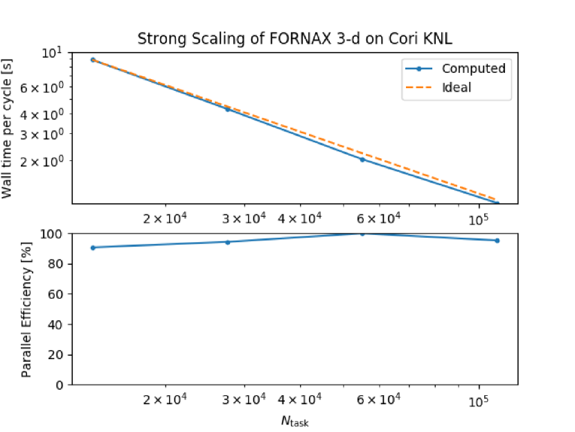
Refer to caption
Figure 31.— This figure demonstrates our code’s raw per-cycle timing (top) and excellent strong scaling efficiency (bottom) out to 110k MPI tasks. Due to the greedy algorithm used to load-balance the decomposition of our dendritic mesh, efficiency can improve with increasing task count as demonstrated here.
Refer to caption
Figure 32.— Top: Wall clock time per time step (in seconds) versus core count for 3-d radiation-hydrodynamic runs. This is a strong scaling test on Blue Waters. Red-dashed is the ideal expectation, and blue is the realization using Fornax. Bottom: The corresponding parallel efficiency versus core count for Fornax (blue) and CASTRO (green). Note that beyond 10,000similar-toabsent10000{\sim}10,000 cores, the efficiency of CASTRO plummets, while that of Fornax maintains high values. At 160,000similar-toabsent160000{\sim}160,000 cores the efficiency of Fornax is still 75similar-toabsent75{\sim}75%. Our efficiencies have improved slightly since this test on Blue Waters was performed (see Fig. 31). Perfect scaling would be a flat curve.

To benchmark the parallel performance of Fornax under production-run conditions, we ran a full radiation-hydrodynamic core-collapse 3-d simulations with 20 energy groups, 12th-order multipole gravity with GR corrections to the monopole component, and a resolution of 608×256×512608256512608\times 256\times 512 (radial, poloidal, toroidal) for 10 cycles with an increasing number of pure MPI tasks out to 110k tasks. The results shown in Figure 31 demonstrate that the code runs extremely fast on NERSC/Cori II, with excellent strong scaling efficiency over 90%. In fact, because of the way we use a greedy algorithm to load-balance the decomposition of our dendritic mesh, the efficiency peaks at larger task count.

Figure 32 demonstrates strong scaling results for Fornax on the Cray/XE6 on Blue Waters for full-star radiation-hydrodynamic simulations using 20 energy groups per neutrino species and 1000×256×51210002565121000\times 256\times 512 spatial gridding in spherical coordinates. We see excellent scaling results to 130,000similar-toabsent130000{\sim}130,000 cores. The lowest efficiency achieved was for 130,000similar-toabsent130000{\sim}130,000 cores and was 75similar-toabsent75{\sim}75%. A comparison was made to the corresponding results for our previous supernova code CASTRO, that requires an iterative transport solution and Krylov subspace methods. After 30,000similar-toabsent30000{\sim}30,000 cores, Fornax is five times more efficient than CASTRO, and after 100,000similar-toabsent100000{\sim}100,000 cores Fornax is approximately ten times as efficient. Moreover, the wallclock and CPU-hour per time step comparisons have revealed that Fornax is also ten times more favorable by these metrics than CASTRO. This comparision is not meant as a criticism of CASTRO, which has many state-of-the-art features and capabilities (Zhang et al. 2011,2013). It merely highlights the differences between an implicit and an explicit treatment of radiative transport in the context of current computer architectures and parallelism modalities.

References

  • Andrews & Spalding (1990) Andrews, M.J. & Spalding, D.B. 1990, Physics of Fluids A: Fluid Dynamics 2, 922
  • Batten et al. (1997) Batten, P., Clarke, N., Lambert, C., & Causon, D.M. 1997, SIAM J. Sci. Comput., 18, 1553
  • Baumgarte et al. (2013) Baumgarte, T.W. and Montero, P.J. and Cordero-Carrión, I. and Müller, E. 2013, Phys. Rev. D87, 044026
  • Berthon et al. (2007) Berthon, C., Charrier, C., & Dubroca, B. 2007, Journal of Scientific Computing, 31, 347
  • Blondin & Lufkin (1993) Blondin, J.M. & Lufkin, E.A. 1993, ApJ88, 589
  • Bruenn et al. (2009) Bruenn, S.W., Mezzacappa, A., Hix, W.R., et al. 2009, Journal of Physics: Conference Series, Volume 180, Issue 1, id. 012018 (arXiv:astro-ph/1002.4914)
  • Bruenn et al. (2016) Bruenn, S.W., Lentz, E.J., Hix, W.R. et al. 2016, ApJ, 818, 123 281
  • Burrows & Thompson (2004) Burrows, A. & Thompson, T.A. 2004, “Neutrino-Matter Interaction Rates in Supernovae, The Essential Microphysics of Core Collapse” in Stellar Collapse, pp. 133-174, ed. C.L. Fryer (Kluwer Academic Publishers; the Netherlands).
  • Burrows (2013) Burrows, A. 2013, \rmp, 85, 245
  • Burrows et al. (2018) Burrows, A., Vartanyan, D., Dolence, J.C., Skinner, M.A., & Radice, D. 2018, Space Science Reviews, 214, 33 (arXiv:1611.058959)
  • Colgate & White (1966) Colgate, S.A., & White, R.H. 1966, ApJ, 143, 626
  • Couch (2013) Couch, S. M. 2013, ApJ, 775, 35
  • Couch & O’Connor (2014) Couch, S.M. & O’Connor, E.P. 2014, ApJ785, 123
  • Davis et al. (2012) Davis, S. Stone, J.M., & Jiang, Y.-F. 2012, ApJS199, 1 (doi:10.1088/0067-0049/199/1/9)
  • Dimonte et al. (2004) Dimonte, G., Youngs, D.L., Dimits, A. et al. 2004, Physics of Fluids, 16, 1668
  • Dubroca & Feugeas (1999) Dubroca, B., & Feugeas, J.L. 1999, CRAS, 329, 915
  • Eswaran & Pope (1988) Eswaran, V. & Pope, S.B. 1988, Computers & Fluids 16, 257
  • Harten, Lax, & van Leer (1983) Harten, A., Lax, P.D., & van Leer, B. 1983, SIAM Rev., 25, 35
  • Hempel & Schaffner-Bielich (2010) Hempel, M. & Schaffner-Bielich, J. 2010, Nucl. Phys. A, 837, 210
  • Hubeny & Burrows (2007) Hubeny, I., & Burrows, A. 2007, ApJ, 659, 1458
  • Kuroda et al. (2012) Kuroda, T., Takiwaki, T., & Kotake, K. 2012, ApJ, 755, 1 (doi:10.1088/0004-637X/755/1/11)
  • Just, Obergaulinger, & Janka (2015) Just, O., Obergaulinger, M., & Janka, H.-T. 2015, MNRAS, 453, 3386 (arXiv:1501.0299)
  • Kamm & Timmes (2007) Kamm, J.R. & Timmes, F.X. 2007, On Efficient Generation of Numerically Robust Sedov Solutions, Tech. Rep. LA-UR-07-2849, Los Alamos National Laboratory
  • Kolb et al. (2013) Kolb, S..M., Stute, M., Kley, W., & Mignone, A. 2013, A&A559, A80
  • Krumholz et al. (2007) Krumholz, M.R., Klein, R.I., McKee, C.F., & Bolstad, J. 2007, ApJ667, 626
  • Lattimer & Swesty (1991) Lattimer, J.M., & Swesty, F. D. 1991, Nucl. Phys., A535, 331
  • Lecoanet et al. (2016) Lecoanet, D., McCourt, M., Quataert, E. et al. 2016, MNRAS, 455, 4274 (arXiv:1509.03630)
  • Liebendörfer et al. (2004) Liebendörfer, M., Messer, O.E.B., Mezzacappa, A., Bruenn, S.W., Cardall, C.Y., & Thielemann, F.-K. 2004, ApJS, 150, 263 1174
  • Liska & Wendroff (2003a) Liska, R. & Wendroff, B., 2003a, SIAM Journal on Scientific Computing, 25, 995
  • Liska & Wendroff (2003b) Liska, R. & Wendroff, B., 2003b, SIAM Journal on Scientific Computing, 25, 3
  • Lowrie & Edwards (2008) Lowrie, R.B. & Edwards, J.D. 2008, Shock Waves 18, 129
  • Marek et al. (2006) Marek, A., Dimmelmeier, H., Janka, H.-T., Müller, E., & Buras, R. 2006, A&A, 445, 273
  • Marek & Janka (2009) Marek, A., & Janka, H.-T. 2009, ApJ, 694, 664
  • Mignone (2014) Mignone, A. 2014, J. Comp. Phys., 270, 784
  • Mönchmeyer & Müller (1989) Mönchmeyer, R., & Müller, E. 1989, A&A, 217, 351
  • Müller & Steinmetz (1995) Müller, E., & Steinmetz, M. 1995, Computer Physics Communications, 89, pp. 45-58
  • Müller et al. (2010) Müller, B., Janka, H.-T., & Dimmelmeier, H. 2010, ApJS, 189, 104
  • Murphy & Burrows (2008a) Murphy, J. W., & Burrows, A. 2008a, ApJ, 688, 1159
  • Murphy & Burrows (2008b) Murphy, J. W., & Burrows, A. 2008b, ApJS, 179, 209 (arXiv:0805.3356)
  • Nagakura et al. (2018) Nagakura, H., Iwakami, W., Furusawa, S., Okawa, H., Harada, A., Sumiyoshi, K., Yamada, S., Matsufuru, H., & Imakura, A., 2018, ApJ854, 136 (arXiv:1702.01752)
  • O’Connor & Couch (2018) O’Connor, E. & Couch, S. 2018, ApJ854, 63 (arXiv:1511.07443)
  • Ott et al. (2012) Ott, C.D., Abdikamalov, E., O’Connor, E., et al. 2012, Phys. Rev. D86, 024026
  • Ott et al. (2013) Ott, C.D., Abdikamalov, E., Mösta, P., Haas, R., Drasco, S., O’Connor, E.P., Reisswig, C., Meakin, C.A., & Schnetter, E. 2013, ApJ, 768, 115 (arXiv:1210.6674)
  • Pope (2000) Pope, S.B. 2000, Turbulent Flows (Cambridge, UK: Cambridge University Press, Sept. 2000) ISBN 0521591252
  • Radice et al. (2017) Radice, D., Abdikamalov, E., Ott, C.D., Mösta, P., Couch, S., & Roberts, L. 2017, (arXiv:1710.01282)
  • Rampp & Janka (2002) M. Rampp, M. & Janka, H.-T. 2002, A&A, 396, 361
  • Roberts et al. (2016) Roberts, L.F., Ott, C.D., Haas, R., O’Connor, E.P., Diener, P., & Schnetter, E. 2016, ApJ, 831, 98
  • Seadrow et al. (2018) Seadrow, S., Burrows, A., Vartanyan, D., Radice, D., & Skinner, M.A. 2018, MNRAS, 480, 4710
  • Sedov (1959) Sedov, L.I. 1959, Similarity and Dimensional Methods in Mechanics (Academic Press)
  • Shibata et al. (2011) Shibata, M., Kiuchi, K., Sekiguchi, Y., & Suwa, Y. 2011, Progress of Theoretical Physics, 125, 1255
  • Shu & Osher (1988) Shu, C.-W. & Osher, S.J. 1988, J. Comput. Phys. 77, 439
  • Skinner, Burrows, & Dolence (2016) Skinner, M.A., Burrows, A., & Dolence, J. 2016, ApJ, 831, 81 (arXiv:1512.00113)
  • Sod (1978) Sod, G. A. 1978, J. Comput. Phys., 27, 1
  • Steiner et al. (2013) Steiner, A.W., Hempel, M., & Fischer, T. 2013, ApJ, 774, 17
  • Stone et al. (2008) Stone, J.M., Gardiner, T.A., Teuben, P., Hawley, J.F., & Simon, J.B. 2008 ApJS, 178, 137
  • Swesty & Myra (2009) Swesty, F.D. & Myra, E.S. 2009, ApJS181, 1
  • Teyssier (2015) Teyssier, R. 2015, ARA&A53, 325
  • Thompson, Burrows & Pinto (2003) Thompson, T.A., Burrows, A., & Pinto, P. 2003, ApJ, 592, 434
  • Toro, Spruce, & Speares (1994) Toro, E.F., Spruce, M., and W. Speares, W. 1994, Shock Waves, 4, 25
  • Typel et al. (2010) Typel, S., Ropke, G., Klahn, T., Blasche, D., & Wolter, H.H. 2010, Phys. Rev. C, 81, 015803
  • Vartanyan et al. (2018) Vartanyan, D., Burrows, A., Radice, D., Skinner, M.A., & Dolence, J.C. 2018, MNRAS, 477, 3091
  • Vaytet et al. (2011) Vaytet, N.M.H., Audit, E., Dubroca, B., & Delahaye, F. 2011, JQSRT, 112, 1323
  • Wallace, Burrows, & Dolence (2016) Wallace, J., Burrows, A., & Dolence, J. 2016, ApJ, 817, 182
  • Weinberg (1972) Weinberg, S. 1972, Graviation and Cosmology: Principles and Applications of the General Theory of Relativity (John Wiley & Sons Inc., New York, 1972), pp. 688. ISBN 0-471-92567-5.
  • Woodward & Colella (1984) Woodward, P. & Colella, P. 1984, J. Comp. Phys. 54, 115
  • Woosley & Heger (2007) Woosley, S. E., & Heger, A. 2007, Phys. Rep., 442, 269
  • Zel’Dovich & Raizer (1969) Zel’Dovich, Y.B. & Raizer, Y.P. 1969, Annual Review of Fluid Mechanics, 1, 385
  • Zhang et al. (2011) Zhang, W., Howell, L., Almgren, A., Burrows, A., & Bell, J. 2011, ApJS, 196, 20
  • Zhang et al. (2013) Zhang, W., Howell, L., Almgren, A., Burrows, A., Dolence, J., & Bell, J. 2013, ApJS, 204, 7