Couplings for determinantal point processes and their reduced Palm distributions with a view to quantifying repulsiveness

Abstract

For a determinantal point process $X$ with a kernel $K$ whose spectrum is strictly less than one, André Goldman has established a coupling to its reduced Palm process $X^{u}$ at a point $u$ with $K(u,u)>0$ so that almost surely $X^{u}$ is obtained by removing a finite number of points from $X$. We sharpen this result, assuming weaker conditions and establishing that $X^{u}$ can be obtained by removing at most one point from $X$, where we specify the distribution of the difference $\xi_{u}:=X\setminus X^{u}$. This is used for discussing the degree of repulsiveness in DPPs in terms of $\xi_{u}$, including Ginibre point processes and other specific parametric models for DPPs.

Jesper Møller and Eliza O’Reilly

[Aalborg University]Jesper MØller [California Institute of Technology]Eliza O’Reilly

Department of Mathematical Sciences, Aalborg University, Skjernvej 4A, 9220 Aalborg Øst, Denmark. Computing and Mathematical Sciences, California Institute of Technology, 1200 E. California Blvd. MC 305-16, Pasadena, CA 91125, USA.

60G55; 60J2060D05; 62M30

1 Introduction

Determinantal point processes (DPPs) have been of much interest over the last many years in mathematical physics and probability theory (see e.g. [5, 11, 17, 26, 28] and the references therein) and more recently in other areas, including statistics [15, 20], machine learning [13], signal processing [6], and neuroscience [27]. They are models for regularity/inhibition/repulsiveness, but there is a trade-off between repulsiveness and intensity [14, 15] (or see Section 4.1.1). This paper sheds further light on this issue by studying various couplings between a DPP and its reduced Palm distributions. In particular, we relate our results to the definition of most repulsive stationary DPPs on $\mathbb{R}^{d}$ as specified in [15, 3]. However, our results will be given for DPPs in a general setting as given below.

Section 2.1.1 provides our general setting for a DPP $X$ defined on a locally compact Polish space $\Lambda$ and specified by a so-called kernel $K:\Lambda\times\Lambda\to\mathbb{C}$ which satisfies certain mild conditions given in Section 2.1.2. Also, for any $u\in\Lambda$ with $K(u,u)>0$, if $X^{u}$ follows the reduced Palm distribution of $X$ at $u$ – intuitively, this is the conditional distribution of $X\setminus\{u\}$ given that $u\in X$ – then $X^{u}$ is another DPP; Section 2.1.3 provides further details. Furthermore, Section 2.2 discusses Goldman’s [9] result that if for any compact set $S\subseteq\Lambda$, denoting $K_{S}$ the restriction of $K$ to $S\times S$, we have that the spectrum of $K_{S}$ is $<1$, then $X$ stochastically dominates $X^{u}$ and hence by Strassen’s theorem there exists a coupling so that almost surely $X^{u}\subseteq X$. The difference $\kappa_{u}:=X\setminus X^{u}$ is a finite point process with a known intensity function. A straightforward calculation also gives that the mean number of points in $\kappa_{u}$ is at most 1, see equations (3) and (4.1.2). In particular, for a standard Ginibre point process [8], which is a special case of a DPP in the complex plane, Goldman showed that $\kappa_{u}$ consists of a single point which follows $N_{\mathbb{C}}(u,1)$, the complex Gaussian distribution with mean $u$ and unit variance. Section 2.3 then discusses some related coupling results due to Pemantle and Peres [24]. One of their results implies that in the specific case where $\Lambda$ is finite, there exists a coupling of $X$ and $X^{u}$ such that $X^{u}\subseteq X$ and the difference is at most one point. However, apart from these and other special cases, the distribution of $\kappa_{u}$ has not been fully characterized.

Section 3 shows that these results can be extended: For a DPP $X$ on any locally compact Polish space $\Lambda$, there is a coupling such that almost surely $X^{u}\subseteq X$, $\xi_{u}:=X\setminus X^{u}$ consists of at most one point, and the distribution of $\xi_{u}$ can be specified. Note that $\kappa_{u}$ and $\xi_{u}$ share the same intensity function, but Goldman did not establish that $\kappa_{u}$ consists of at most one point. As in [9] we only verify the existence of our coupling result. We leave it as an open research problem to provide a specific coupling construction or simulation procedure for $(X,X^{u})$ (restricted to a compact subset of $\Lambda$), hence extending the simulation algorithm for a DPP [10, 14, 15, 20].

Section 4 discusses how our coupling result can be used for describing the repulsiveness in a DPP, including when considering the notion of a globally most repulsive DPP by which we mean that for all $u\in\Lambda$ with $K(u,u)>0$, almost surely $\xi_{u}$ has one point. For example, if $X$ is a standard Ginibre point process, we obtain a similar result as in [9]: $X$ is a globally most repulsive DPP and the point in $\xi_{u}$ follows $N_{\mathbb{C}}(u,1)$. In particular, we show that our definitions extend those given in [15, 3] for stationary DPPs on $\mathbb{R}^{d}$, and by considering the distribution of the point in $\xi_{u}$, we demonstrate how the range of repulsion can differ with DPPs that have the same intensity and the same global repulsiveness. Moreover, we consider the cases of a finite set $\Lambda$ and when we have a stationary DPP defined on $\Lambda=\mathbb{R}^{d}$. Finally, we compare with globally most repulsive isotropic DPPs on $\mathbb{S}^{d}$, the $d$-dimensional unit sphere in $\mathbb{R}^{d+1}$, as studied in [19].

2 Background

This section provides the background material needed in this paper.

2.1 Setting

Below we give the definition of a DPP, specify our assumptions, and recall that the reduced Palm distribution of a DPP is another DPP.

2.1.1 Definition of a DPP

Let $X$ be a point process defined on a locally compact Polish space $\Lambda$ equipped with its Borel $\sigma$-algebra $\mathcal{B}$ and a Radon measure $\nu$ which is used as a reference measure in the following. We assume that $X$ is a DPP with kernel $K$ which by definition means the following. First, $X$ has no multiple points, so dependent on the context we view $X$ as a random subset of $\Lambda$ or as a random counting measure, and we let $X(B)$ denote the cardinality of $X_{B}:=X\cap B$ for $B\in\mathcal{B}$. Second, $K$ is a complex function defined on $K:\Lambda^{2}\mapsto\mathbb{C}$. Third, for any $n=1,2,\ldots$ and any mutually disjoint bounded sets $B_{1},\ldots,B_{n}\in\mathcal{B}$,

$$\mathrm{E}\left[X\left(B_{1}\right)\cdots X\left(B_{n}\right)\right]=\int_{B_{1}\times\cdots\times B_{n}}\det\left\{K\left(u_{i},u_{j}\right)\right\}_{i,j=1}^{n}\,\mathrm{d}\nu^{n}\left(u_{1},\ldots,u_{n}\right)$$

is finite, where $\nu^{n}$ denotes the $n$-fold product measure of $\nu$. This means that $X$ has $n$-th order intensity function $\rho(u_{1},\ldots,u_{n})$ (also sometimes in the literature called $n$-th order correlation function) given by the determinant

$$\rho\left(u_{1},\ldots,u_{n}\right)=\det\left\{K\left(u_{i},u_{j}\right)\right\}_{i,j=1}^{n},\qquad u_{1},\ldots,u_{n}\in\Lambda,$$ (1)

and this function is locally integrable. In particular, $\rho(u)=K(u,u)$ is the intensity function of $X$, and when $B\in\mathcal{B}$ is bounded almost surely $X_{B}$ is finite.

In the special case where $K(u,v)=0$ whenever $u\not=v$, the DPP $X$ is just a Poisson process with intensity function $\rho(u)$ conditioned on that there are no multiple points in $X$ (if $\nu$ is diffuse, it is implicit that there are no multiple points). For other examples when $\Lambda$ is a countable set and $\nu$ is the counting measure, see [13]; when $\Lambda=\mathbb{R}^{d}$ and $\nu$ is the Lebesgue measure, see [11, 15]; and when $\Lambda=\mathbb{S}^{d}$ (the $d$-dimensional unit sphere) and $\nu$ is the surface/Lebesgue measure, see [19]. Examples are also given in Section 4.2.

From (1) and the fact that the determinant of a complex covariance matrix is less than or equal to the product of its diagonal elements we obtain that

$$\rho\left(u_{1},\ldots,u_{n}\right)\leq\prod_{i=1}^{n}\rho\left(u_{i}\right),$$

where the equality holds if and only if $X$ is a Poisson process. Thus, apart from the case of a Poisson process, the counts $X(A)$ and $X(B)$ are negatively correlated whenever $A,B\in\mathcal{B}$ are disjoint.

2.1.2 Assumptions

We always make the following assumptions (a)–(c):

1. $K$ is Hermitian, that is, $K(u,v)=\overline{K(v,u)}$ for all $u,v\in\Lambda$;

2. $K$ is locally square integrable, that is, for any compact set $S\subseteq\Lambda$, the double integral $\int_{S}\int_{S}|K(u,v)|^{2}\,\mathrm{d}\nu(u)\,\mathrm{d}\nu(v)$ is finite;

3. $K$ is of locally trace class, that is, for any compact set $S\subseteq\Lambda$, the integral $\int_{S}K(u,u)\,\mathrm{d}\nu(u)$ is finite.

By Mercer’s theorem, excluding a $\nu^{2}$-nullset, this ensures the existence of a spectral representation for the kernel restricted to any compact set $S\subseteq\Lambda$: Ignoring a $\nu^{2}$-nullset, we can redefine $K$ on $S\times S$ by

$$K(u,v)=\sum_{k=1}^{\infty}\lambda_{k}^{S}\phi_{k}^{S}(u)\overline{\phi_{k}^{S}(v)}\qquad u,v\in S,$$ (2)

where the eigenvalues $\lambda_{k}^{S}$ are real numbers and the eigenfunctions $\phi_{k}^{S}$ constitute an orthonormal basis of $L^{2}(S)$, cf. Section 4.2.1 in [11]. Here, for any $B\in\mathcal{B}$, $L^{2}(B)=L^{2}(B,\nu)$ is the space of square integrable complex functions w.r.t. $\nu$ restricted to $B$. Note that (c) means $\mathrm{E}X(S)=\sum_{k=1}^{\infty}\lambda_{k}^{S}<\infty$. Thus, when $B\in\mathcal{B}$ is bounded, almost surely $X_{B}$ is finite. When $\nu$ is diffuse, as we are redefining $K$ by (2) we have effectively excluded the special case of the Poisson process (i.e. when $K$ is 0 off the diagonal) because all the eigenvalues in (2) are then 0; however, as shown later, it will still make sense to consider the Poisson process when quantifying repulsiveness in DPPs.

We also always assume that

1. for any compact set $S\subseteq\Lambda$, all eigenvalues satisfy $0\leq\lambda_{k}^{S}\leq 1$.

In fact, under (a)–(c), the existence of the DPP with kernel $K$ is equivalent to (d) (see e.g. Theorem 4.5.5 in [11]), and the DPP is then unique (Lemma 4.2.6 in [11]). If $\Lambda=\mathbb{R}^{d}$, $\nu$ is the Lebesgue measure, and $K(u,v)=K_{0}(u-v)$ is stationary, where $K_{0}\in L^{2}(\mathbb{R}^{d})$ and $K_{0}$ is continuous, we denote the Fourier transform of $K_{0}$ by $\hat{K}_{0}$. Then (d) is equivalent to $0\leq\hat{K}_{0}\leq 1$ (Proposition 3.1 in [11]).

Recalling that $K_{S}$ is the restriction of $K$ to $S\times S$, we sometimes consider one of the following conditions:

1. For a given compact set $S\subseteq\Lambda$, $K_{S}$ is a projection of finite rank $n$.

2. For all compact $S\subseteq\Lambda$, all eigenvalues satisfy that $\lambda_{k}^{S}<1$.

2.1.3 Reduced Palm distributions

Consider an arbitrary point $u\in\Lambda$ with $\rho(u)>0$. Recall that the reduced Palm distribution of $X$ at $u$ is a point process $X^{u}$ on $\Lambda$ with $n$-th order intensity function

$$\rho^{u}(u_{1},\ldots,u_{n})=\rho(u,u_{1},\ldots,u_{n})/\rho(u).$$

This combined with (1) easily shows that $X^{u}$ is a DPP with kernel

$$K^{u}(v,w)=K(v,w)-\frac{K(v,u)K(u,w)}{K(u,u)}\qquad v,w\in\Lambda,$$ (3)

see Theorem 6.5 in [26]. For any compact set $S\subseteq\Lambda$, it follows that the restriction $X^{u}_{S}:=X^{u}\cap S$ follows the reduced Palm distribution of $X_{S}$ at $u$.

2.2 Goldman’s results

Goldman [9] made similar assumptions as in our assumptions (a)-(d), and in addition he assumed condition (f) throughout his paper. Two of his main results were the following.

1. For any $u\in\Lambda$ with $K(u,u)>0$, there is a coupling of $X$ and $X^{u}$ so that almost surely $X^{u}\subseteq X$.

2. Suppose $X$ is a standard Ginibre point process, that is, the DPP on $\Lambda=\mathbb{C}\equiv\mathbb{R}^{2}$, with $\nu$ being Lebesgue measure, and with kernel

   $$K(v,w)=\frac{1}{\pi}\exp\left(v\overline{w}-\frac{|v|^{2}+|w|^{2}}{2}\right),\qquad v,w\in\mathbb{C}.$$ (4)

   Then, for the coupling in (G1) and any $u\in\mathbb{C}$, $X\setminus X^{u}$ consists of a single point which follows $N_{\mathbb{C}}(u,1)$.

It follows from (G1) and (3) that $\kappa_{u}:=X\setminus X^{u}$ is a finite point process with intensity function

$$\rho_{\kappa_{u}}(v)={|K(u,v)|^{2}}/{K(u,u)},\qquad v\in\Lambda.$$ (5)

Note that the standard Ginibre point process is stationary and isotropic with intensity $1/\pi$, but its kernel is not of the form $K(u,v)=K_{0}(\|u-v\|)$. In accordance with (G2), combining (4) and (5), $\rho_{\kappa_{u}}$ is immediately seen to be the density of $N_{\mathbb{C}}(u,1)$.

2.3 Pemantle and Peres’ results

Pemantle and Peres [24] studied probability measures on $\{0,1\}^{n}$ satisfying a negative dependence property called the strong Rayleigh property. This class of probability measures was introduced in [4], where it was also shown that determinantal point processes on a finite set satisfy this property. In [24], the authors define notions called stochastic covering and the stochastic covering property, which can be defined as follows. Letting $X$ and $Y$ be simple point processes, $X$ is said to stochastically cover $Y$ if there is a coupling $(X,Y)$ such that $X=Y$ or their difference $X\setminus Y$ is one point. Now, consider a simple point process $X$ on a finite set $\Lambda=\{1,\ldots,n\}$. Then, $X$ is said to have the stochastic covering property if the following holds. If $u\in x\subseteq S\subseteq\Lambda$ and we set $y=x\setminus\{u\}$, then the point process $X_{S^{c}}$ conditioned on $X_{S}=x$ is stochastically covered by the point process $X_{S^{c}}$ conditioned on $X_{S}=y$. This property implies for $u\in\{1,\ldots,n\}$ (letting $S=x=\{u\}$) that the point process $X\setminus\{u\}$ conditioned on $u\notin X$ stochastically covers $X^{u}$, and in turn that $X$ stochastically covers $X^{u}$.

Proposition 2.2 in [24] states that for a probability measure on $\{0,1\}^{n}$, the strong Rayleigh property implies the stochastic covering property, and thus determinantal point processes on $\Lambda=\{1,\ldots,n\}$ satisfy this property. The authors discuss extensions to the case where $\Lambda$ is continuous, and in particular they extend their Proposition 2.3 to this case. However, a generalization of their Proposition 2.2 to the case of continuous determinantal point processes does not appear in the most recent version [24]. As kindly pointed out by a referee, in the first version of this paper on arXiv [23], the authors claim $X$ stochastically covers $X^{u}$ in the continuous case as well, and the main idea of our proof of Theorem 3.3 below is outlined. However, their justification is not complete for our general setting.

3 Main result

The theorem below is our main result which is sharpening Goldman’s result (G1) in that we do not assume condition (f) and we establish a coupling so that $X$ stochastically covers $X^{u}$. It also sharpens Pemantle and Peres’ result since it holds for a general locally compact Polish space $\Lambda$. In addition, we completely describe the distribution of the difference $X\backslash X^{u}$. In the proof of the theorem we use basic results and definitions for operators on the Hilbert space $\mathcal{L}^{2}(\Lambda)$, see e.g. [21, 22]. An outline of the proof is as follows. First, we dilate the operator associated to the DPP $X$ to a projection operator on the union of two copies of $\Lambda$. Second, we use the existence of a coupling for projection operators in Lemma 3.1. Finally, we compress back down to $\Lambda$ to obtain the desired coupling.

We use the following special result established under condition (e) and where $\nu_{S}$ denotes the restriction of the reference measure $\nu$ to a compact set $S\subseteq\Lambda$.

Lemma 3.1.

Assume $S\subseteq\Lambda$ is compact and let $\{\phi^{S}_{k}\}_{k=1}^{n}$ be an orthonormal set of functions in $L^{2}(S)$ with $1\leq n<\infty$. Let $X$ and $Y$ be DPPs with kernels $K$ and $L$, respectively, so that

$$K(v,w)=\sum_{k=1}^{n}\phi^{S}_{k}(v)\overline{\phi^{S}_{k}(w)},\qquad L(v,w)=\sum_{k=1}^{n-1}\phi^{S}_{k}(v)\overline{\phi^{S}_{k}(w)},\qquad v,w\in S$$

(setting $L(v,w)=0$ if $n=1$). Then there exists a monotone coupling of $Y_{S}$ w.r.t. $X_{S}$ such that almost surely $Y_{S}\subset X_{S}$, $\eta_{S}:=X_{S}\setminus Y_{S}$ consists of one point, and the point in $\eta_{S}$ has density $|\phi^{S}_{n}(\cdot)|^{2}$ w.r.t. $\nu_{S}$.

Proof 3.2.

Observe that $K$ and $L$ are the kernels of finite dimensional projections, a special case of trace-class positive contractions, and the difference,

$$K(v,w)-L(v,w)=\phi^{S}_{n}(v)\overline{\phi^{S}_{n}(w)},\qquad v,w\in S,$$

is a positive definite kernel. Thus, by Theorem 3.8 in [16], $X_{S}$ stochastically dominates $Y_{S}$. Therefore, there is a coupling such that almost surely $Y_{S}\subseteq X_{S}$. As $Y_{S}$ has cardinality one less than $X_{S}$, almost surely $\eta_{S}:=X_{S}\setminus Y_{S}$ consists of one point. Finally, for any Borel set $A\subseteq S$,

$$\mathrm{P}(\eta_{S}\cap A\not=\emptyset)=\mathrm{E}\left[1_{\{X(A)-Y(A)=1\}}\right]=\mathrm{E}[X(A)]-\mathrm{E}[Y(A)]=\int_{A}|\phi^{S}_{n}(v)|^{2}\,\mathrm{d}\nu(v).$$

Denote $\|\cdot\|_{2}$ the usual norm on $\mathcal{L}^{2}(\Lambda)$ w.r.t. $\nu$.

Theorem 3.3.

Let $X$ be a DPP on $\Lambda$ with kernel $K$ satisfying conditions (a)–(d). For any $u\in\Lambda$ with $K(u,u)>0$, there exists a coupling of $X$ and $X^{u}$ such that almost surely $X^{u}\subseteq X$ and $\xi_{u}:=X\setminus X^{u}$ consists of at most one point. We have

$$p_{u}:=\mathrm{P}(\xi_{u}\neq\emptyset)=\frac{1}{K(u,u)}\int|K(u,v)|^{2}\,\mathrm{d}\nu(v),$$ (6)

and conditioned on $\xi_{u}\neq\emptyset$ the point in $\xi_{u}$ has density

$$f_{u}(v):={|K(u,v)|^{2}}/{\|K(u,\cdot)\|_{2}^{2}},\qquad v\in\Lambda,$$ (7)

w.r.t. $\nu$.

Compared to Goldman’s result (G1), we also have $p_{u}=\mathrm{P}(\kappa_{u}\not=\emptyset)$ and $f_{u}$ is the conditional density of a point in $\kappa_{u}$ given that $\kappa_{u}\not=\emptyset$, cf. (5)–(7).

Proof 3.4.

We begin by describing the procedure given in Lyons’ paper [16, Section 3.3] for dilating a locally trace class operator to a locally trace class orthogonal projection. Denote $\mathcal{K}$ the locally trace class operator on $\mathcal{L}^{2}(\Lambda)$ with kernel $K$. Consider the dilation of $\mathcal{K}$ given by

$$\mathcal{Q}:=\begin{bmatrix}\mathcal{K}&\mathcal{L}\\ \mathcal{L}&\mathcal{I}-\mathcal{K}\end{bmatrix},$$

where $\mathcal{L}:=\sqrt{\mathcal{K}(\mathcal{I}-\mathcal{K})}$. Then, since $Q=Q^{2}$, $Q$ is an orthogonal projection on $L^{2}(\Lambda,\nu)\oplus L^{2}(\Lambda_{0},\nu)$, where $\Lambda_{0}$ is a disjoint identical copy of $\Lambda$. If $\Lambda$ is discrete, then $Q$ is clearly locally trace class, since any compact set of a discrete space is finite. If $\Lambda$ is not discrete, consider the operator

$$\mathcal{Q}^{\prime}:=\begin{bmatrix}\mathcal{I}&0\\ 0&\mathcal{U}\end{bmatrix}^{*}\mathcal{Q}\begin{bmatrix}\mathcal{I}&0\\ 0&\mathcal{U}\end{bmatrix}=\begin{bmatrix}\mathcal{K}&\mathcal{L}\mathcal{U}\\ \mathcal{U}^{*}\mathcal{L}&\mathcal{U}^{*}(\mathcal{I}-\mathcal{K})\mathcal{U}\end{bmatrix},$$

where $\mathcal{U}$ is a unitary operator from $\ell^{2}(\Lambda_{0}^{\prime})$ to $L^{2}(\Lambda_{0},\nu)$ for some countably infinite space $\Lambda_{0}^{\prime}$. The operator $\mathcal{U}$ exists since any two infinite dimensional separable Hilbert spaces are unitarily equivalent. The operator $\mathcal{Q}^{\prime}$ is an orthogonal projection on $L^{2}(\Lambda,\nu)\oplus\ell^{2}(\Lambda_{0}^{\prime})$, and $\mathcal{K}$ is the compression of $\mathcal{Q}^{\prime}$ to $\Lambda$. Further, $\mathcal{Q}^{\prime}$ is also locally trace class, because $\mathcal{K}$ is locally trace class on $L^{2}(\Lambda,\nu)$ by assumption, and all operators on $\ell^{2}(\Lambda_{0}^{\prime})$ are locally of trace class since $\Lambda_{0}^{\prime}$ is discrete. Thus, $\mathcal{Q}^{\prime}$ defines a projection DPP $Y_{Q}$ on the union $\Lambda\cup\Lambda_{0}^{\prime}$.

First, assume that $\Lambda$ is compact. Then, the kernel of the operator $\mathcal{K}$ satisfies

$$K(v,w)=\sum_{k\geq 1}\lambda^{\Lambda}_{k}\phi^{\Lambda}_{k}(v)\overline{\phi^{\Lambda}_{k}(w)},\qquad v,w\in\Lambda,$$

where $\{\phi^{\Lambda}_{k}\}$ is an orthonormal basis for $L^{2}(\Lambda)$, $\lambda^{\Lambda}_{k}\in[0,1]$ for all $k$, and $\sum_{k\geq 1}\lambda^{\Lambda}_{k}<\infty$. Also, the kernel for the operator $\mathcal{L}$ is then given by

$$L(v,w)=\sum_{k\geq 1}\sqrt{\lambda^{\Lambda}_{k}(1-\lambda^{\Lambda}_{k})}\phi^{\Lambda}_{k}(v)\overline{\phi^{\Lambda}_{k}(w)}.$$

Note that

$$\mathcal{L}(L(\cdot,u))(w)=\int_{\Lambda}L(w,v)L(v,u)\,\mathrm{d}\nu(v)=\sum_{k\geq 1}\lambda^{\Lambda}_{k}(1-\lambda^{\Lambda}_{k})\phi^{\Lambda}_{k}(w)\overline{\phi^{\Lambda}_{k}(u)},$$

and

$$\mathcal{K}(K(\cdot,u))(w)=\int_{\Lambda}K(w,v)K(v,u)\,\mathrm{d}\nu(v)=\sum_{k\geq 1}\left(\lambda^{\Lambda}_{k}\right)^{2}\phi^{\Lambda}_{k}(w)\overline{\phi^{\Lambda}_{k}(u)}.$$

Hence, $\mathcal{K}(K(\cdot,u))+\mathcal{L}(L(\cdot,u))=K(\cdot,u)$. Also,

$$\mathcal{L}(K(\cdot,u))(w)=\int_{\Lambda}L(w,v)K(v,u)\,\mathrm{d}\nu(v)=\sum_{k\geq 1}\lambda^{\Lambda}_{k}\sqrt{\lambda^{\Lambda}_{k}(1-\lambda^{\Lambda}_{k})}\phi^{\Lambda}_{k}(w)\overline{\phi^{\Lambda}_{k}(u)}$$

and

$$\mathcal{K}(L(\cdot,u))(w)=\int_{\Lambda}K(w,v)L(v,u)\,\mathrm{d}\nu(v)=\sum_{k\geq 1}\lambda^{\Lambda}_{k}\sqrt{\lambda^{\Lambda}_{k}(1-\lambda^{\Lambda}_{k})}\phi^{\Lambda}_{k}(w)\overline{\phi^{\Lambda}_{k}(u)},$$

and so $\mathcal{L}(K(\cdot,u))=\mathcal{K}(L(\cdot,u))$. Consequently, for fixed $u\in\Lambda$,

$$\psi_{u}(\cdot):=\begin{bmatrix}\frac{K(\cdot,u)}{\sqrt{K(u,u)}}\\ \mathcal{U}^{*}\left(\frac{L(\cdot,u)}{\sqrt{K(u,u)}}\right)\end{bmatrix}$$

is an eigenvector of the operator $\mathcal{Q}^{\prime}$. Indeed, since $\mathcal{U}\mathcal{U}^{*}=\mathcal{I}$ by that fact that $\mathcal{U}$ is unitary,

$$\mathcal{Q}^{\prime}(\psi_{u}(\cdot)) =\begin{bmatrix}\mathcal{I}&0\\ 0&\mathcal{U}\end{bmatrix}^{*}Q\begin{bmatrix}\frac{K(\cdot,u)}{\sqrt{K(u,u)}}\\ (\mathcal{U}\mathcal{U}^{*})\left(\frac{L(\cdot,u)}{\sqrt{K(u,u)}}\right)\end{bmatrix}$$

$$=\begin{bmatrix}\mathcal{I}&0\\ 0&\mathcal{U}^{*}\end{bmatrix}\begin{bmatrix}\frac{\mathcal{K}(K(\cdot,u))}{\sqrt{K(u,u)}}+\frac{\mathcal{L}(L(\cdot,u))}{\sqrt{K(u,u)}}\\ \frac{\mathcal{L}(K(\cdot,u))}{\sqrt{K(u,u)}}+\frac{(\mathcal{I}-\mathcal{K})(L(\cdot,u))}{\sqrt{K(u,u)}}\end{bmatrix}=\begin{bmatrix}\frac{K(\cdot,u)}{\sqrt{K(u,u)}}\\ \mathcal{U}^{*}\left(\frac{L(\cdot,u)}{\sqrt{K(u,u)}}\right)\end{bmatrix}=\psi_{u}(\cdot).$$

Then, we can define the projection

$$\mathcal{Q}_{u}^{\prime}:=\mathcal{Q}^{\prime}-P_{\psi_{u}},$$

where $P_{\psi_{u}}$ is the projection operator on $L^{2}(\Lambda,\nu)\oplus\ell^{2}(\Lambda_{0}^{\prime})$ onto the span of $\psi_{u}$. This projection operator is also locally trace class since it is the difference of locally trace class operators. Then we can define the projection DPP $Y_{Q}^{u}$ on $\Lambda\cup\Lambda_{0}^{\prime}$ associated with $\mathcal{Q}_{u}^{\prime}$. If $\mathcal{Q}^{\prime}$ has finite rank, then $\mathcal{Q}^{\prime}$ and $\mathcal{Q}_{u}^{\prime}$ have corresponding kernels

$$Q^{\prime}=\sum_{k=0}^{n}q_{k}q_{k}^{T}\quad\text{ and }\quad Q_{u}^{\prime}=\sum_{k=1}^{n}q_{k}q_{k}^{T},$$

where $n<\infty$, $\{q_{k}\}_{k=1}^{n}$ is an orthonormal set, and $q_{0}:=\psi_{u}$. Applying Lemma 3.1 then gives the result.

Now, assume $\mathcal{Q}^{\prime}$ projects onto an infinite dimensional subspace of $L^{2}(\Lambda,\nu)\oplus\ell^{2}(\Lambda_{0}^{\prime})$ and let $\{q_{k}\}_{k=0}^{\infty}$ be an orthonormal basis for the range of $\mathcal{Q}^{\prime}$, where $q_{0}:=\psi_{u}$. For each positive integer $M$, define the finite dimensional projection kernels

$$Q_{M}^{\prime}=\sum_{k=0}^{M}q_{k}q_{k}^{T}\quad\text{ and }\quad Q_{M,u}^{\prime}=\sum_{k=1}^{M}q_{k}q_{k}^{T},$$

and let $Y_{Q_{M}}$ and $Y^{u}_{Q_{M}}$ be the corresponding projection DPPs. By Lemma 3.1, there is a coupling of $Y_{Q_{M}}$ and $Y_{Q_{M}}^{u}$ such that almost surely $Y_{Q_{M}}\supset Y^{u}_{Q_{M}}$, where $\xi_{Q_{M}}^{u}:=Y_{Q_{M}}\setminus Y^{u}_{Q_{M}}$ consists of one point which has density $|\psi_{u}(\cdot)|^{2}$. By the same argument as in the proof of Lemma 20 in [9], the sequences $Y_{Q_{M}}$ and $Y^{u}_{Q_{M}}$ are tight and converge in distribution to $Y_{Q}$ and $Y^{u}_{Q}$, respectively, as $M\to\infty$. Also, the sequence $(Y^{u}_{Q_{M}},\xi_{Q_{M}}^{u})_{M}$ is tight, and thus a subsequence converges in distribution to $(Y^{u}_{Q},\xi^{u}_{Q})$, where $\xi^{u}_{Q}$ consists of one point with density $|\psi_{u}(\cdot)|^{2}$, and $Y^{u}_{Q}\cup\xi^{u}_{Q}$ is equal in distribution to $Y_{Q}$.

The projection operator $P_{\psi_{u}}$ has kernel $\psi_{u}\psi_{u}^{T}$ and the compression of $P_{\psi_{u}}$ to $\Lambda$ is the integral operator with kernel

$$\frac{K(v,u)K(u,w)}{K(u,u)}.$$

Then, since the compression of $\mathcal{Q}^{\prime}$ to $\Lambda$ is the operator $\mathcal{K}$, the compression of $\mathcal{Q}_{u}^{\prime}$ to $\Lambda$ is the integral operator $\mathcal{K}^{u}$ with kernel

$$K^{u}(v,w)=K(v,w)-\frac{K(v,u)K(u,w)}{K(u,u)}.$$

This gives that $Y_{Q}\cap\Lambda$ has the same distribution as $X$ and $Y^{u}_{Q}\cap\Lambda$ has the same distribution as $X^{u}$. Thus, almost surely

$$X=X^{u}\cup\xi_{u},$$

where $\xi_{u}:=\xi_{Q}^{u}\cap\Lambda$ and $X^{u}$ are disjoint. Therefore, we have a coupling of $X$ and $X^{u}$, where almost surely $X^{u}\subseteq X$ and the difference is at most one point. The probability of $\xi_{u}\neq\emptyset$ is the probability that $\xi^{u}_{Q}$ is in $\Lambda$, and the density of $\xi^{u}_{Q}$ restricted to $\Lambda$ is

$$f_{\xi^{u}_{Q}}(v)1_{\{v\in\Lambda\}}=\frac{|K(v,u)|^{2}}{K(u,u)}$$

w.r.t. $\nu$. Hence,

$$\mathrm{P}(\xi^{u}\neq\emptyset)=\mathrm{P}(\xi^{u}_{Q}\in\Lambda)=\int\frac{|K(v,u)|^{2}}{K(u,u)}\,\mathrm{d}\nu(v)$$

and the density of $\xi_{u}$ conditioned on $\xi_{u}\neq\emptyset$ is $f_{u}(v)={|K(v,u)|^{2}}/{\|K(\cdot,u)\|_{2}^{2}}$ w.r.t. $\nu$.

Second, if $\Lambda$ is not assumed to be compact, consider a sequence of compact sets $S_{n}\subset\Lambda$ such that $\cup_{n=1}^{\infty}S_{n}=\Lambda$ and $S_{n}\subseteq S_{n+1}$ for $n=1,2,\ldots$. For each $n$, using the result above with $\Lambda$ replaced by $S_{n}$, there exists a coupling of $(X_{S_{n}},X_{S_{n}}^{u})$, where almost surely $X_{S_{n}}=X_{S_{n}}^{u}\cup\xi^{u}_{S_{n}}$, $\xi^{u}_{S_{n}}=X_{S_{n}}\setminus X_{S_{n}}^{u}$ consists of at most one point,

$$\mathrm{P}\left(\xi^{u}_{S_{n}}\neq\emptyset\right)=\int_{S_{n}}\frac{|K(v,u)|^{2}}{K(u,u)}\,\mathrm{d}\nu(v),$$ (8)

and conditioned on $\xi^{u}_{S_{n}}\neq\emptyset$ the density of the point in $\xi^{u}_{S_{n}}$ is

$$f_{u,S_{n}}(v)=|K(v,u)|^{2}/\int_{S_{n}}|K(w,u)|^{2}\,\mathrm{d}\nu(w)$$ (9)

w.r.t. $\nu_{S_{n}}$. For consistency, let $T_{1}=S_{1}$ and generate a realization $(y_{T_{1}},y^{u}_{T_{1}})$ of $(Y_{T_{1}},Y^{u}_{T_{1}}):=(X_{S_{1}},X^{u}_{S_{1}})$, and for $n=2,3,\ldots$, let $T_{n}=S_{n}\setminus S_{n-1}$ and generate a realization $(y_{T_{n}},y^{u}_{T_{n}})$ of $(Y_{T_{n}},Y^{u}_{T_{n}})$ which follows the conditional distribution of $(X_{S_{n}}\setminus S_{n-1},X^{u}_{S_{n}}\setminus S_{n-1})$ given that $(X_{S_{n}}\cap S_{n-1},X^{u}_{S_{n}}\cap S_{n-1})=(\cup_{i=1}^{n-1}y_{T_{i}},\cup_{i=1}^{n-1}y^{u}_{T_{i}})$. Then $(X,X^{u})$ is distributed as $(Y,Y^{u}):=(\cup_{n=1}^{\infty}Y_{T_{n}},\cup_{n=1}^{\infty}Y^{u}_{T_{n}})$, and almost surely, for $n=2,3,\ldots$, $Y_{T_{n-1}}\setminus Y^{u}_{T_{n-1}}\not=\emptyset$ implies that $Y_{T_{n}}\setminus Y^{u}_{T_{n}}=Y_{T_{n+1}}\setminus Y^{u}_{T_{n+1}}=\ldots=\emptyset$, and so $\xi_{u}:=Y\setminus Y^{u}$ consists of at most one point. The probability that $\xi_{u}$ is non-empty is, by (8),

$$\mathrm{P}(\xi_{u}\neq\emptyset)=\lim_{n\to\infty}\int_{S_{n}}\frac{|K(v,u)|^{2}}{K(u,u)}\,\mathrm{d}\nu(v)$$

and hence by monotone convergence we obtain (6). Finally, (7) is obtained in a similar way using (9).

4 Describing repulsiveness in DPPs

In this section we use the probability $p_{u}$ to quantify how repulsive a DPP can be, and we use the density $f_{u}$ from Theorem 3.3 to describe the repulsive effect of a fixed point contained in a DPP. As mentioned in Section 4.1, in the case of stationary DPPs on $\mathbb{R}^{d}$, $p_{u}$ turns out to agree with a measure for repulsiveness studied in [15, 14, 3, 2], but we are not aware of references where $f_{u}$ has been considered when discussing repulsiveness in DPPs. Examples of $p_{u}$ and $f_{u}$ for specific models of DPPs are given in Section 4.2.

Note that $X^{u}$ is the point process where there is a ‘ghost point’ at $u$ that is affecting the remaining points. Using this coupling of $X^{u}$ and $X$, it is clear that the repulsive effect of a point at location $u$ is characterized by the difference between $X^{u}$ and the original DPP $X$, where there is no repulsion coming from the location $u$. Further, as $X$ and $X^{u}$ have intensity functions $\rho(\cdot)$ and $\rho(u,\cdot)/\rho(u)$, respectively, $\xi_{u}=X\setminus X^{u}$ has intensity function

$$\rho_{u}(v):={|K(v,u)|^{2}}/{K(u,u)},\qquad v\in\Lambda.$$

This is the intensity function for the points in $X$ ‘pushed out’ by $u$ under the Palm distribution. It makes also sense to consider $\rho_{u}$ as the intensity function of $X\setminus X^{u}$ when $\nu$ is diffuse and $X$ is a Poisson process because then $X=X^{u}$ and $\rho_{u}(v)=0$ for $v\not=u$.

4.1 A measure of repulsiveness

Setting $0/0=0$, recall that the pair correlation function of $X$ is defined by $g(v,w)=\rho(v,w)/(\rho(v)\rho(w))$ for $v,w\in\Lambda$, so it satisfies

$$1-g(v,w)=|r(v,w)|^{2},\qquad v,w\in\Lambda,$$

where $r(v,w)=K(v,w)/\sqrt{K(v,v)K(w,w)}$ is the correlation function obtained from $K$. Note that

$$\rho_{u}(v)=\rho(v)(1-g(u,v)),\qquad v\in\Lambda.$$ (10)

4.1.1 Defining a global measure of repulsiveness

As a global measure of repulsiveness in $X$ when having a point of $X$ at $u$, we suggest the probability of $\xi_{u}\not=\emptyset$, that is,

$$p_{u}=\int\rho_{u}(v)\,\mathrm{d}\nu(v)=\int{|K(u,v)|^{2}}/{K(u,u)}\,\mathrm{d}\nu(v).$$

By (10), there is a trade-off between intensity and repulsiveness: If $p_{u}$ is fixed, we cannot both increase $\rho$ and decrease $g$. Therefore, when using $p_{u}$ as a measure to compare repulsiveness in two DPPs, they should share the same intensity function $\rho$. Then small/high values of $p_{u}$ correspond to small/high degree of repulsiveness. For a stationary DPP $X$ on $\mathbb{R}^{d}$, $p_{u}$ agrees with the measure for repulsiveness in DPPs introduced in [15, 14]; see also [3, 2]. Indeed this measure is very specific for DPPs as discussed later in Section 4.2.5.

4.1.2 Definition of globally most repulsive DPPs

If $p_{u}=1$ for all $u\in\Lambda$ with $K(u,u)>0$, we say that $X$ is a globally most repulsive DPP. This is the case if $K$ is a projection, that is, for all $v,w\in\Lambda$,

$$K(v,w)=\int K(v,y)K(y,w)\,\mathrm{d}\nu(y).$$

For short we then say that $X$ is a projection DPP. The standard Ginibre point process given by (4) is globally most repulsive, and its kernel is indeed a projection; this follows from a straightforward calculation using that $(v,w)\to\exp(v\overline{w})$ is the reproducing kernel of the Bargmann-Fock space equipped with the standard complex Gaussian measure. At the other end, if $\nu$ is diffuse and $X$ is a Poisson process with intensity function $\rho$, then $p_{u}=0$ for all $u\in\Lambda$ with $\rho(u)>0$, and so $X$ is a globally least repulsive DPP.

If $\Lambda$ is compact, then it follows from the spectral representation (2) and condition (d) that

$$\int_{S}|K(u,v)|^{2}\,\mathrm{d}\nu(v)= \sum_{k}\sum_{\ell}\lambda^{S}_{k}\lambda^{S}_{l}\phi^{S}_{k}(u)\overline{\phi^{S}_{\ell}(u)}\int_{S}\overline{\phi^{S}_{k}(v)}\phi^{S}_{\ell}(v)\,\mathrm{d}\nu(v)$$

$$= \sum_{k}\left(\lambda^{S}_{k}\right)^{2}|\phi^{S}_{k}(u)|^{2}\leq\sum_{k}\lambda^{S}_{k}|\phi^{S}_{k}(u)|^{2}=K(u,u),$$ (11)

and so

$$p_{u}=\frac{\sum_{k}\left(\lambda^{\Lambda}_{k}\right)^{2}|\phi^{\Lambda}_{k}(u)|^{2}}{\sum_{k}\lambda^{\Lambda}_{k}|\phi^{\Lambda}_{k}(u)|^{2}}.$$ (12)

Consequently, in this case, projection DPPs are the only globally most repulsive DPPs. Such a process has a fixed number of points which agrees with the rank of the kernel.

4.2 Examples

This section shows specific examples of our measure $p_{u}$ and the distribution of a point in $\xi_{u}$.

4.2.1 DPPs defined on a finite set

Assume $\Lambda=\{1,\ldots,n\}$ is finite and $\nu$ is the counting measure; this is the simplest situation. Then $L^{2}(\Lambda)\equiv\mathbb{C}^{n}$, the class of possible kernels for DPPs corresponds to the class of $n\times n$ complex covariance matrices with all eigenvalues $\leq 1$, and the eigenfunctions simply correspond to normalized eigenvectors for such matrices. For simplicity we only consider projection DPPs and Poisson processes below, but other examples of DPPs on finite sets include uniform spanning trees (Example 14 in [11]) and finite DPPs converging to the continuous Airy process on the complex plane [12].

The projection DPPs are given by complex projection matrices, ranging between the degenerated cases where $X=\emptyset$ and $X=\Lambda$. For example, consider the projection kernel of rank two given by $K(v,w)=\frac{1}{n}+t_{v}\overline{t_{w}}$, where $\sum_{i=1}^{n}t_{i}=0$ and $\sum_{i=1}^{n}|t_{i}|^{2}=1$. For any $u\in\{1,\ldots,n\}$, we have $p_{u}=1$ and

$$\rho_{u}(v)=\frac{|\frac{1}{n}+t_{u}\overline{t_{v}}|^{2}}{\frac{1}{n}+|t_{u}|^{2}},\qquad v\in\{1,\ldots,n\},$$

is a probability mass function. This shows the repulsive effect of having a point of $X$ at $u$; in particular, $\rho_{u}(v)$ has a global maximum point at $v=u$.

The kernel of a Poisson process with intensity function $\rho\leq 1$ and conditioned on having no multiple points is given by a diagonal covariance matrix with diagonal entries $\rho(1),\ldots,\rho(n)$. If $\rho(u)>0$, then $p_{u}=\rho(u)$. This is a much different result as when we consider a Poisson process $X$ on a space $\Lambda$ where the reference measure $\nu$ is diffuse: If $\rho(u)>0$, then $p_{u}=0$ and almost surely $X=X^{u}$.

4.2.2 Ginibre point processes

From the standard Ginibre point process given by (4), other stationary point processes can be obtained. Independently thinning the process with a retention probability $\alpha\beta$, where $\beta>0$ and $\alpha\in(0,1/\beta]$, and multiplying each of the retained points by $\sqrt{\beta}$ gives a new stationary DPP with kernel

$$K(v,w)=\frac{\alpha}{\pi}\exp\left(\frac{v\overline{w}}{\beta}-\frac{|v|^{2}+|w|^{2}}{2\beta}\right),\qquad v,w\in\mathbb{C}.$$ (13)

We have

$$\rho={\alpha}/{\pi},\qquad p_{u}=\alpha\beta,\qquad f_{u}(v)=\frac{\exp\left(-|v-u|^{2}/\beta\right)}{\pi\beta}\sim N_{\mathbb{C}}(u,\beta).$$ (14)

The case where $\alpha=1$ and $0<\beta\leq 1$ is mentioned in Goldman’s paper [9], and the results in (14) match those in Remark 24 in [9]. [6] called the DPP with kernel (13) the scaled $\beta$-Ginibre point process but the bound $\alpha\beta\leq 1$ was not noticed. For any fixed value of $\rho>0$, as the value of $\beta$ increases to its maximum $\min\{1,1/(\pi\rho)\}$, the more repulsive the process becomes, whilst as $\beta$ decreases to 0, in the limit a Poisson process with intensity $\rho$ is obtained.

4.2.3 DPPs on $\mathbb{R}^{d}$ with a stationary kernel

Suppose $\Lambda=\mathbb{R}^{d}$, $\nu$ is the Lebesgue measure, and $K(u,v)=K_{0}(u-v)$ is stationary, where $K_{0}\in L^{2}(\mathbb{R}^{d})$ and $K_{0}$ is continuous. Then it follows from Parseval’s identity that $p_{u}=1$ if and only if $\hat{K}_{0}$ is an indicator function whose integral agrees with the intensity of $X$, cf. Appendix J in [14]. A natural choice for the support of this indicator function is a ball centred at the origin in $\mathbb{R}^{d}$, and if (as in the standard Ginibre point process) we let the intensity be $1/\pi$, then the globally most repulsive DPP has a stationary and isotropic kernel given by

$$K(v,w)=\int_{|y|^{d}\leq d\Gamma(d/2)/(2\pi^{1+d/2})}\exp\left(2\pi i(v-w)\cdot y\right)\,\mathrm{d}y,\qquad v,w\in\mathbb{R}^{d},$$ (15)

where $x\cdot y$ denotes the usual inner product for $x,y\in\mathbb{R}^{d}$ and $|y|$ is the usual Euclidean distance. For instance, for $d=1$ this kernel is the sinc function and for $d=2$ it is the jinc-like function

$$K(v,w)=J_{1}(2|v-w|)/(\pi|v-w|),$$ (16)

where $J_{1}$ is the Bessel function of order one. We straightforwardly obtain the following proposition, where the moments in (17) follow from Eq. 10.22.57 in [1].

Proposition 1.

For the globally most repulsive DPP on $\mathbb{R}^{d}$ with kernel given by (15) and for any $u\in\mathbb{C}$, we have that $\rho_{u}(v)=\pi|K(u,v)|^{2}$ is a probability density function. In particular, for $d=2$,

$$\rho_{u}(v)=J_{1}(2|v-u|)^{2}/\left(\pi|v-u|^{2}\right),\qquad v\in\mathbb{R}^{2},$$

and the moments of $|Z_{u}-u|$ with $Z_{u}\sim\rho_{u}$ satisfy

$$\mathrm{E}\left(|Z_{u}-u|^{k}\right)=\frac{\Gamma(1+k/2)\Gamma(1-k)}{\Gamma(2-k/2)\Gamma(1-k/2)^{2}},\qquad k\in(-2,1),$$ (17)

and are infinite for $k\geq 1$.

For comparison consider a standard Ginibre point process, where we can define $Z_{u}$ in a similar way as in Proposition 1. In both cases, $|Z_{u}-u|$ is independent of $(Z_{u}-u)/|Z_{u}-u|$, which is uniformly distributed on the unit circle. However, the distribution of $|Z_{u}-u|$ is very different in the two cases: For the standard Ginibre point process, $|Z_{u}-u|^{2}$ is exponentially distributed and $|Z_{u}-u|$ has a finite $k$-th moment for all $k>-2$ given by $\Gamma(1+k/2)/(\pi\rho)^{k/2}$; whilst for the DPP on $\mathbb{R}^{2}$ with jinc-like kernel (16), $|Z_{u}-u|$ is heavy-tailed and has infinite $k$-th moments for all $k\geq 1$.

For any DPP $X$ with kernel $K$ and defined on $\mathbb{R}^{d}$, using independent thinning and scale transformation procedures similar to those in Section 4.2.2 (replacing $\sqrt{\beta}$ by $\beta^{1/d}$ when transforming the points in the thinned process), we obtain a new DPP with kernel

$$K_{\mathrm{new}}(v,w)=\alpha K(v/\beta^{1/d},w/\beta^{1/d}),\qquad v,w\in\mathbb{R}^{d},$$

where $\beta\in(0,1]$ and $\alpha\in(0,1/\beta]$. For instance, if $K$ is the jinc-like kernel for the globally most repulsive DPP given by (16), the new DPP satisfies the same equations for its intensity $\rho$ and its probability $p_{u}$ as in (14). Hence, if $\rho$ and $\beta$ are the same for this new DPP and the scaled $\beta$-Ginibre point process, the two DPPs are equally repulsive in terms of $p_{u}$. However, the probability density function for the point in $\xi_{u}$ conditioned on $\xi_{u}\not=\emptyset$ now becomes

$$f_{u}(v)=J_{1}\left(2|v-u|^{2}/\beta\right)/\left(\pi|v-u|^{2}/\beta\right).$$ (18)

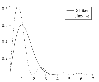
The reach of the repulsive effect of the point at $u$ is much different when comparing the densities in (14) and (18), in particular if $\beta$ is large. See Figure 1 for a comparison of the densities (14) and (18) for $\beta=1$.

Figure 1: The densities of $|Z_{0}|$ for $Z_{0}:=X\backslash X^{0}$ for two globally most repulsive DPPs.

4.2.4 DPPs on $\mathbb{S}^{d}$ with an isotropic kernel

Suppose $\Lambda=\mathbb{S}^{d}$ is the $d$-dimensional unit sphere, $\nu$ is the Lebesgue measure, and $K(v,w)=K_{0}(v\cdot w)$ is isotropic for all $v,w\in\mathbb{S}^{d}$. Then the DPP with kernel $K$ is isotropic, and $\rho=K_{0}(1)$ and $p_{u}$ do not depend on the choice of $u\in\Lambda$. By a classical result of Schoenberg [25] and by Theorem 4.1 in [19], we have the following. The normalized eigenfunctions will be complex spherical harmonic functions, and $K_{0}$ will be real and of the form

$$K_{0}(t)=\rho\sum_{\ell=0}^{\infty}\beta_{\ell,d}\frac{C_{\ell}^{\left(\frac{d-1}{2}\right)}(t)}{C_{\ell}^{\left(\frac{d-1}{2}\right)}(1)},\qquad-1\leq t\leq 1,$$

where $C_{\ell}^{\left(\frac{d-1}{2}\right)}$ is a Gegenbauer polynomial of degree $\ell$ and the sequence $\beta_{0,d},\beta_{1,d},\ldots$ is a probability mass function. Further, letting $\sigma_{d}=\nu(\mathbb{S}^{d})=2\pi^{(d+1)/2}/\Gamma((d+1)/2)$, the eigenvalues of $K$ are

$$\lambda_{\ell,d}=\rho\sigma_{d}\beta_{\ell,d}/m_{\ell,d},\qquad\ell=0,1,\ldots,$$

with multiplicities

$$m_{0,1},\qquad m_{\ell,1}=2,\qquad\ell=1,2,\ldots,\qquad\mbox{if }d=1,$$

and

$$m_{\ell,d}=\frac{2\ell+d-1}{d-1}\frac{(\ell+d-2)!}{\ell!(d-2)!},\qquad\ell=0,1,\ldots,\qquad\mbox{if }d\in\{2,3,\ldots\}.$$

So the DPP exists if and only if $\rho\leq\inf_{\ell:\,\beta_{\ell,d}>0}m_{\ell,d}/(\sigma_{d}\beta_{\ell,d})$. Now, applying (12), we obtain

$$p_{u}=\rho\sigma_{d}\sum_{\ell=0}^{\infty}\beta_{\ell,d}^{2}/m_{\ell,d}.$$ (19)

There is a lack of flexible parametric DPP models on the sphere where $K_{0}$ is expressible in closed form, see Section 4.3 in [19]. For instance, let $d=2$ and consider the special case of the multiquadric model given by

$$K_{0}(t)=\rho\frac{1-\delta}{\sqrt{1+\delta^{2}-2\delta t}},\qquad-1\leq t\leq 1,$$

with $\delta\in(0,1)$ a parameter and $0<\rho\leq 1/(4\pi(1-\delta))$. Then, as shown in Section 4.3.2 in [19], the sequence

$$\beta_{\ell,2}=(1-\delta)\delta^{\ell},\qquad\ell=0,1,\ldots,$$ (20)

specifies a geometric distribution and

$$\lambda_{\ell,2}=4\pi\rho\delta^{\ell}(1-\delta)/(2\ell+1)\leq\delta^{\ell}/(2\ell+1),\qquad\ell=0,1,\ldots.$$

As $\delta\rightarrow 0$, then $\lambda_{0,2}\rightarrow 4\pi\rho$ and $\lambda_{\ell,2}\rightarrow 0$ if $\ell\geq 1$, corresponding to the uninteresting case of a DPP with at most one point if $\rho<1/(4\pi)$ and with exactly one point if $\rho=1/(4\pi)$. From (19) and (20) we obtain

$$p_{u}=4\pi\rho(1-\delta)/(1+\delta)\leq 1/(1+\delta),$$

with this upper bound obtained for the maximal value of $\rho=1/(4\pi(1-\delta))$. Therefore the DPP with the multiquadric kernel is far from being globally most repulsive unless the expected number of points is very small.

Instead a flexible parametric model for the eigenvalues $\lambda_{\ell,d}$ is suggested in Section 4.3.4 in [19] so that globally most repulsive DPPs as well as Poisson processes are obtained as limiting cases. However, the disadvantage of that model is that we can only numerically calculate $\rho$ and $p_{u}$.

4.2.5 Remark

The considerations in Sections 4.1 and 4.2.1-4.2.4 are strictly for DPPs. For example, the intensity function of a Gibbs point process can be both smaller and larger than the intensity function of its Palm distribution at a given point; whilst for a DPP, $\rho\geq\rho^{u}$. Furthermore, as a candidate for a ‘globally most repulsive stationary Gibbs point process on $\mathbb{R}^{2}$’, we may consider $Y=L_{Z}:=\{x+Z:x\in L\}$, where $L$ is the vertex set of a regular triangular lattice (the centres of a honeycomb structure) with one lattice point at the origin, and where $Z$ is a uniformly distributed point in the hexagonal region given by the Voronoi cell of the lattice and centred at the origin (in other words, $Y$ may be considered as the limit of a stationary Gibbs hard core process when the packing fraction of hard discs increases to the maximal value $\approx 0.907$, see e.g. [7, 18]). However, the reduced Palm process at $u\in\mathbb{R}^{2}$ will be degenerated and given by $Y^{u}=L_{u}\setminus\{u\}$, which is a much different situation as compared to DPPs.

Jesper Møller was supported in part by The Danish Council for Independent Research | Natural Sciences, grant 7014-00074B, ‘Statistics for point processes in space and beyond’, and by the ‘Centre for Stochastic Geometry and Advanced Bioimaging’, funded by grant 8721 from the Villum Foundation. Eliza O’Reilly was supported in part by a grant of the Simons Foundation (#197982 to UT Austin), the National Science Foundation Graduate Research Fellowship under Grant No. DGE-1110007, and the Department of Mathematical Sciences, Aalborg University. We are grateful to Professor Russell Lyons for many useful comments, in particular for changing our focus on a more complicated coupling result established in an earlier version of our paper (briefly, to obtain the reduced Palm process, one point in the DPP was either moved or removed) to the simpler coupling result in Theorem 3.3, which indeed is more suited for studying repulsiveness in DPPs. Also, he pointed our attention to his paper [16], which is essential in the proof of Theorem 3.3. Finally, we are grateful to two referees, in particular for pointing our attention to the work by Pemantle and Peres.

References

• [1] NIST Digital Library of Mathematical Functions. http://dlmf.nist.gov/, Release 1.0.14 of 2017-09-18. F. W. J. Olver, A. B. Olde Daalhuis, D. W. Lozier, B. I. Schneider, R. F. Boisvert, C. W. Clark, B. R. Miller and B. V. Saunders, eds.
• [2] Baccelli, F. and O’Reilly, E. (2018). Reach of repulsion for determinantal point processes in high dimensions. Journal of Applied Probability 55, 760–788.
• [3] Biscio, C. A. N. and Lavancier, F. (2016). Quantifying repulsiveness of determinantal point processes. Bernoulli 22, 2001–2028.
• [4] Borcea, J., BrΓ€ndΓ©n, P. and Liggett, T. (2009). Negative dependence and the geometry of polynomials. Journal of the American Mathematical Society 22, 521–567.
• [5] Borodin, A. and Olshanski, G. (2000). Distributions on partitions, point processes and the hypergeometric kernel. Communications in Mathematical Physics 211, 335–358.
• [6] Deng, N., Zhou, W. and Haenggi, M. (2015). The Ginibre point process as a model for wireless networks with repulsion. IEEE Transactions on Wireless Communications 14, 107–121.
• [7] DΓΆge, G., Mecke, K., MΓΈller, J., Stoyan, D. and Waagepetersen, R. (2004). Grand canonical simulations of hard-disk systems by simulated tempering. International Journal of Modern Physics C 15, 129–147.
• [8] Ginibre, J. (1965). Statistical ensembles of complex, quaternion, and real matrices. Journal of Mathematical Physics 6, 440–449.
• [9] Goldman, A. (2010). The Palm measure and the Voronoi tessellation for the Ginibre process. Annals of Applied Probability 20, 90–128.
• [10] Hough, J. B., Krishnapur, M., Peres, Y. and VirΓ g, B. (2006). Determinantal processes and independence. Probability Surveys 3, 206–229.
• [11] Hough, J. B., Krishnapur, M., Peres, Y. and VirΓ g, B. (2009). Zeros of Gaussian Analytic Functions and Determinantal Point Processes. American Mathematical Society, Providence.
• [12] Johansson, K. (2005). The arctic circle boundary and the airy process. The Annals of Probability 33, 1–30.
• [13] Kulesza, A. and Taskar, B. (2012). Determinantal Point Processes for Machine Learning. Now Publishers Inc., Hanover, MA, USA.
• [14] Lavancier, F., MΓΈller, J. and Rubak, E. (2014). Determinantal point process models and statistical inference (extended version). Technical report. Available on arXiv:1205.4818.
• [15] Lavancier, F., MΓΈller, J. and Rubak, E. (2015). Determinantal point process models and statistical inference. Journal of the Royal Statistical Society: Series B (Statistical Methodology) 77, 853–877.
• [16] Lyons, R. (2014). Determinantal probability: Basic probability and conjectures. Proceedings of International Congress of Mathematicians IV, 137–161.
• [17] Macchi, O. (1975). The coincidence approach to stochastic point processes. Advances in Applied Probability 7, 83–122.
• [18] Mase, S., MΓΈller, J., Stoyan, D., Waagepetersen, R. and DΓΆge, G. (2001). Packing densities and simulated tempering for hard core Gibbs point processes. Annals of the Institute of Statistical Mathematics 53, 661–680.
• [19] MΓΈller, J., Nielsen, M., Porcu, E. and Rubak, E. (2018). Determinantal point process models on the sphere. Bernoulli 24, 1171–1201.
• [20] MΓΈller, J. and Rubak, E. (2016). Functional summary statistics for point processes on the sphere with an application to determinantal point processes. Spatial Statistics 18, 4–23.
• [21] Nagy, B. S., Foias, C., Bercovici, H. and KΓ©rchy, L. (2010). Harmonic Analysis of Operators on Hilbert Space. Springer-Verlag, New York.
• [22] Paulsen, V. (2002). Completely Bounded Maps and Operator Algebras. Cambridge University Press, Cambridge.
• [23] Pemantle, R. and Peres, Y. (2011). Concentration of lipschitz functionals of determinantal and other strong rayleigh measures. arXiv:1108.0687v1.
• [24] Pemantle, R. and Peres, Y. (2014). Concentration of lipschitz functionals of determinantal and other strong rayleigh measures. Combinatorics, Probability, and Computing 23, 140–160.
• [25] Schoenberg, I. J. (1942). Positive definite functions on spheres. Duke Mathematical Journal 9, 96–108.
• [26] Shirai, T. and Takahashi, Y. (2003). Random point fields associated with certain Fredholm determinants I: fermion, Poisson and boson point processes. Journal of Functional Analysis 205, 414–463.
• [27] Snoek, J., Zemel, R. S. and Adams, R. P. (2013). A determinantal point process latent variable model for inhibition in neural spiking data. In Advances in Neural Information Processing Systems 26 (NIPS 2013). ed. I. S. Francis, B. J. F. Manly, and F. C. Lam. Electronic proceedings from the conference, "Neural Information Processing Systems 2013". pp. 1932–1940.
• [28] Soshnikov, A. (2000). Determinantal random point fields. Russian Mathematical Surveys 55, 923–975.