NuSTAR rules out a cyclotron line in the accreting magnetar candidate 4U2206$+$54.

Abstract

Based on our new NuSTAR X-ray telescope data, we rule out any cyclotron line up to 60 keV in the spectra of the high mass X-ray binary 4U2206$+$54. In particular, we do not find any evidence of the previously claimed line around 30 keV, independently of the source flux, along the spin pulse. The spin period has increased significantly, since the last observation, up to $5750\pm 10$ s, confirming the rapid spin down rate $\dot{\nu}=-1.8\times 10^{-14}$ Hz s^-1. This behaviour might be explained by the presence of a strongly magnetized neutron star ($B_{\rm s}>$ several times $10^{13}$ G) accreting from the slow wind of its main sequence O9.5 companion.

1 Introduction

The existence of accreting magnetars is an open question of modern Astrophysics. Magnetars are powered by magnetic energy. These isolated neutron stars harbour the strongest cosmic magnets with field strengths in the $10^{13-15}$ G range (Thompson & Duncan, 1993). A wide range of high-energy phenomena displayed by Soft Gamma-ray Repeaters and Anomalous X-Ray Pulsars are explained by the extreme physics of magnetars (Thompson et al., 2002; Thompson & Beloborodov, 2005; Woods & Thompson, 2006). About 30 magnetars and candidates are now known (Olausen & Kaspi, 2014), but none of them is an accreting neutron star (NS).

An NS is a remnant of a massive star with $M_{\rm initial}>8\,M_{\odot}$. The vast majority of massive stars are binaries (Chini et al., 2012; Sana et al., 2012). Only a small fraction of these binaries remain bound after the primary explodes as a supernova but the number of such systems in the Galaxy is still quite large (Liu et al., 2006). The accretion of the stellar wind onto the NS powers a strong X-ray luminosity in these high-mass X-ray binaries (HMXBs). In our current understanding on how binary systems evolve (e.g. van den Heuvel & De Loore, 1973; Postnov & Yungelson, 2014), and given the magnetic field strength distribution of known pulsars (Olausen & Kaspi, 2014, Fig.7), a (small) fraction of HMXBs should host neutron stars with magnetar strength fields, i.e., being accreting magnetars. Yet, the very existence of the class is unclear.

A handful of accreting magnetar candidates have now been proposed, among them the long period X-ray pulsars 4U0114$+$65 (Sanjurjo-Ferrrín et al., 2017) and AX J1910.7$+$0917 (Sidoli et al., 2017). The magnetar nature of our target, 4U2206$+$54, has been suggested on the grounds of its very long spin period ($P_{s}=5560$ s, the third largest known after AX J1910.7$+$0917 and 4U0114$+$65) and a very high period derivative, $\dot{\nu}=-1.5\pm 0.2\times 10^{-14}$ Hz s^-1 (Finger et al., 2010; Reig et al., 2012) which would drive the NS to a complete halt in $\Delta t\gtrsim 300$ yr. The possible explanations involve NS spin magneto-braking in a magnetic field exceeding $B\sim 10^{13}$ G (e.g. Ikhsanov & Beskrovnaya, 2010).

However, the magnetar nature of the neutron star in 4U2206$+$54 has been disputed because the extant low signal to noise X-ray spectra do not rule out the presence of a cyclotron resonant scattering feature (CRSF; from now on, a cyclotron line) at $E_{\rm cyc}\approx 29$ keV, a clear signature of a magnetic field of $B=3.3\times 10^{12}$ G, definitely not in the magnetar range. Although at a quite low significance, the detection has been claimed on the basis of spectra obtained with several satellites (Beppo SAX , RXTE , INTEGRAL ) and at different epochs (Torrejón et al., 2004; Blay et al., 2005; Wang, 2009). If this line is indeed present in the X-ray spectra, the system contains no magnetar. Further constraints have then to be added in order to accomodate the pronounced spin down. Ikhsanov & Beskrovnaya (2013) propose the magnetic accretion model. This mechanism requires a (low) magnetization of the donor stellar wind. In such a case, a dense magnetic slab of ambient matter forms around the magnetosphere of the NS, able to remove the angular momentum at the observed rate even for normal strength magnetic fields ($B\sim 10^{12}$ G). However, a joint analysis of (non contemporaneous) XMM-Newton and INTEGRAL data, did not reveal the presence of any cyclotron line (Reig et al., 2012), casting serious doubts on its existence.

The goal of this paper is to confirm or rule out such a line. To that end we present an analysis of a 58.6 ks NuSTAR observation of 4U2206$+$54 covering, for the first time, the energy range from 3 to 60 keV with no spectral gaps. The high S/N ratio provides a stringent test to the presence of a cyclotron line.

The paper is structured as follows: in Section 2 we present the observational details. In sections 3 and 4 we analyze the light curve and flux resolved spectra of the source, providing the best fit parameters for the continuum. Finally, in Sections 5 and 6 we discuss these parameters in the framework of the theory and present the conclusions.

2 Observations

Table 1: Observations journal

ObsID	Date	$t_{\rm exp}$	$\phi_{\rm orb}$
30201015002	2016-05-17 09:51:08a	58.6	0.03 (0.22)b

• MJD 57525.41050926

• Time for X-ray maximum $T_{0}=51856.6\pm 0.1$ MJD (Ribó et al., 2006). Phases for orbital periods $P=9.5591\pm 0.0007$ d and $P=19.25\pm 0.08$ d Corbet et al. (2007), respectively.

We observed 4U2206$+$54 with NuSTAR on 17 May 2016 during 58.6 ks on target. In Table 1 we specify the observation journal details. The NuSTAR data were extracted with the standard software nupipeline v1.7.1, which is part of HEASOFT v6.20. We used CALDB version 20170222. The data were extracted from a circular region with radius of 100^′′ centred on the brightest pixels in the image after standard screening. The background was extracted from a circular region with a radius of 150^′′ located as far away from the source as possible within the field of view. We also extracted data from the SCIENCE_SC mode, during which the pointing is less precise (see, e.g. Walton et al., 2016), adding about 15% exposure time. We used a circular region with $90^{\prime\prime}$ radius to extract the source spectra and lightcurves from these data and a similar background region as in the standard data. All data were corrected for the solar system barycentered using the DE200 ephemeris. The spectral analysis was performed with the Interactive Spectral Interpretation System (isis) v 1.6.1-24 (Houck & Denicola, 2000).

3 Light curves and timing analysis

We extracted energy resolved lightcurves between 3–5 keV, 5–10 keV, and 10–79 keV with 10 s time resolution and a broadband lightcurve between 3–79 keV with 1 s time resolution. Figure 1 shows the NuSTAR background subtracted light curve in the energy range 5-10 keV with a bin size of 60 s. In this energy band, the source shows the highest count rate while the effects of photoelectric absorption are minimized. The light curve is strongly variable as typical in wind accreting HMXBs. This stochastic variation is superimposed to the pulse of the NS. The relatively large amplitude variations are due to the pulsations, as can be seen in the inset.

Table 2: Spin period determination.

Method	$P_{\rm spin}$ (s)
Fundamental
Lomb-Scargle	$5750\pm 10$
PDM	$5741\pm 38$
CLEAN	$5752\pm 38$
CHISQ	$5740\pm 68$
Mean	5746$\pm$6
Weighted mean	5752$\pm$9
Final adopted value	5750$\pm$10

Figure 1: $5-10$ keV light curve of 4U 2204+54. The inset shows a more detailed view of the variability. Strong evidence for pulsations is seen. Time zero corresponds to JD 2,457,525.912

The determination of the spin period in 4U 2204+54 with NuSTAR data is difficult owing to the structure of the light curve and the sampling of the periodicity. Due to the low-Earth orbit, NuSTAR data are affected by the passage near the South Atlantic Anomaly and suffers from Earth occultations. Therefore the light curve contains numerous gaps interspersed with continue data segments. The observation spans over $\sim$108 ks, but the total on-source time was 58.6 ks. Although the data segments are evenly sampled (bin size of 10 s), the spin period of 4U 2204+54 is longer than the typical duration of each data segment. In other words, the phase coverage of the observed signal is incomplete.

Under these conditions, the use of Fourier techniques is inappropriate. The good news is that we know the value of the periodicity, hence we do not need to perform a blind search and we can restrict the relevant frequency range. The latest reported value of the spin period of 4U 2204+54 is 5593 s, obtained from an XMM-Newton observation in 2011 (Reig et al., 2012). They derived a spin-down rate of $(1.5\pm 0.2)\times 10^{-14}$ Hz s^-1. If we assume that this rate continued until the NuSTAR observation on JD 2457525.91, then the expected period would be $\sim 5690$ s. We note that the orbital period of the satellite is 5828 s.

We based our analysis on the the Lomb-Scargle periodogram (LSP) (Lomb, 1976; Scargle, 1982). There are various implementations of the LSP. The differences appear in the normalization of the periodogram, whether the zero point of the sinusoid is allowed to change during the fit (Cumming et al., 1999), the treatment of errors (Zechmeister & Kürster, 2009), and in the computation speed (Press & Rybicki, 1989; Townsend, 2010).

Figure 2: Lomb-Scargle periodograms of the 5–10 keV light curve of 4U 2204+54 using different implementations of the algorithm. Top: sample mean as in the original Lomb-Scargle periodogram. Middle: Python implementation allowing the model fits for the mean of the data. Bottom Power spectrum of the window function.

The upper panel of Fig. 2 shows the LSP using the original formulation of pre-centering the data to the sample mean. Two peaks are apparent. The first peak at $\nu=0.0001739$ Hz and the second peak at twice that frequency. Although the first frequency is close to the expected period, its power is significantly lower than the second peak. The reason for the suppression of the power of the fundamental peak is the use of the sample mean in a time series when the data do not provide full phase coverage of the observed signal (VanderPlas, 2017). In the middle panel of Fig. 2 we show the LSP using the floating mean method, which involves adding an offset term to the sinusoidal model at each frequency (Cumming et al., 1999; Zechmeister & Kürster, 2009). The average spin period obtained from the LSP is $5750\pm 10$ s. The error was estimated from the dispersion of the different values obtained after running the various implementations of the Lomb-Scargle periodogram. We confirmed the high significance of the peak by calculating the false alarm probability (the detection threshold above which the signal is significant) through bootstrap analysis. We find that the peak is significant well above 99.99%.

Figure 3: Simulated light curve with $P=5750$ s (upper panels). Below each lightcurve, the LSP and window spectrum for different selections of $T_{\rm data}$ and $T_{\rm gaps}$, are shown. See text for details.

To examine the conditions under which the suppression of the main peak occurs, we simulated a purely sinusoidal signal affected by Poisson noise with a period of $P_{\rm spin}=5750$ s. Then we removed data points at regular intervals, each interval with a duration of $T_{\rm gaps}$, leaving continuous stretches of data of duration $T_{\rm data}$. This is illustrated in Fig. 3, where two cases which differ in the value of $T_{\rm data}$ and $T_{\rm gaps}$ are shown. In both cases we assume that $T_{\rm data}+T_{\rm gaps}=P_{\rm spin}$.

In the left and middle columns of Fig. 3, $T_{\rm data}=3350$ s, $T_{\rm gaps}=2400$ s and $T_{\rm data}=4000$ s, $T_{\rm gaps}=1750$ s, respectively. A strong peak is apparent in the window spectrum at a frequency $1/(T_{\rm data}+T_{\rm gaps})$, which in this case is equal to $1/P_{\rm spin}$. When the data segments do not cover a good fraction of the pulse phase, $T_{\rm data}/P_{\rm spin}=0.6$, the power of the peak that corresponds to the true period is suppressed (left column, signal panel). As the phase coverage increases ($T_{\rm data}/P_{\rm spin}$ approaches 1), the power of the true period increases (middle column, signal panel).

We also performed a simulation using the exact exposure window of the observations (right column in Fig. 3). In this case, the light curve was created by replicating the pulse profile to cover the length of the observation. Poisson noise was added to each bin. The pulse profile was obtained using the derived period of 5750 s. Then we introduced gaps using the same good time intervals as the real light curve. The first peak appears at the expected frequency. In the real light curve and the simulated one using the real good time intervals, the peak of the window power spectrum appears at $\nu=0.0001721$ Hz ($P=5811$ s), while the spin period occurs at $\nu=0.0001739$ Hz ($P=5750$ s). These simulations give us confidence that the peak at frequency $\sim$0.0001739 Hz in the LSP of 4U 2204+54 is real and corresponds to the true period.

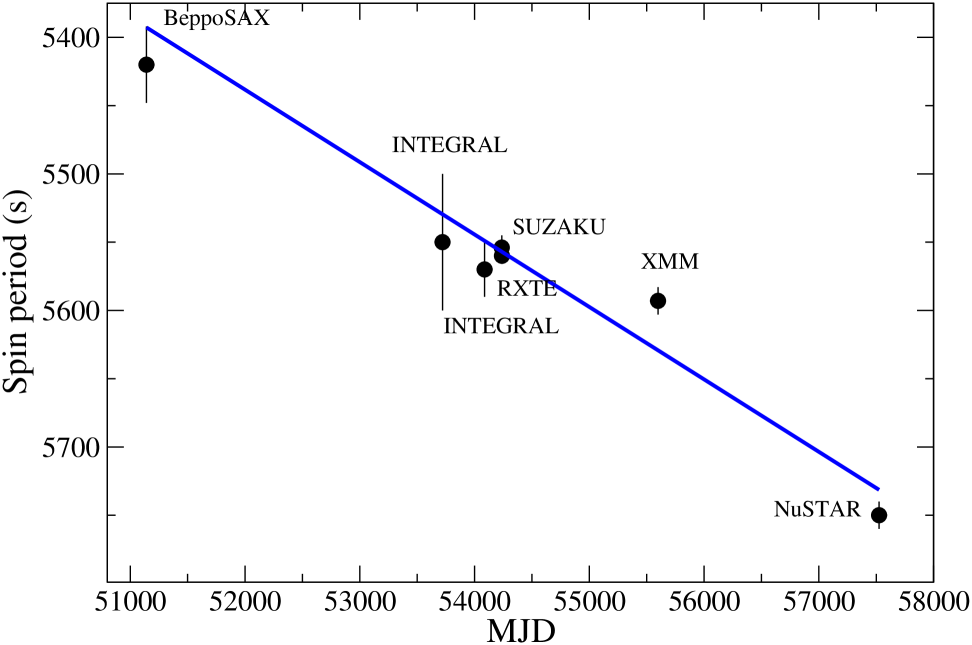
Figure 4: Spin period evolution of 4U 2204+54. The best linear fit is $P_{\rm spin}=2680+0.053*MJD$, with errors $\sigma_{y}=160$ and $\sigma_{x}=0.003$.

We compared the average spin period obtained from the LSP value with those obtained using other techniques such as the clean (Roberts et al., 1987), the phase dispersion minimization (pdm Stellingwerf, 1978) algorithms and $\chi^{2}$ minimization. These algorithms are implemented in the program PERIOD (version 5.0), distributed with the starlink Software Collection. Note that the final "clean" spectrum of the clean deconvolution algorithm detects only the first harmonic. The reason is that the clean algorithm assumes that the highest peak in the periodogram corresponds to the primary signal. Table 2 summarizes the results of the period search. We took the result from the LSP as the final adopted value of the spin period of 4U 2204+54. The timing analysis was performed using the 5–10 keV light curve. However, the analysis performed at other energy ranges gave consistent results.

Figure 4 shows the evolution of the spin period of 4U 2204+54 over the past 20 years. Data prior to the NuSTAR observation were taken from Reig et al. (2012). A linear fit to the data represents a good approximation of the long-term variation of the spin period with time. The source continues to spin down at a rate of $(1.8\pm 0.1)\times 10^{-14}$ Hz s^-1. This value agrees with previous reported values $(1.7\pm 0.3)\times 10^{-14}$ Hz s^-1 (Finger et al., 2010) and $(1.5\pm 0.2)\times 10^{-14}$ Hz s^-1 (Reig et al., 2012).

In Fig, 5 we show the average spin pulse folded over the NuSTAR period, $5750\pm 10$ s, for several energy ranges. It shows a double peak structure. Several emission flux levels are identified and separated by vertical lines. These will be used to perform flux resolved spectroscopy in the next section.

4 Spectra

The observed X-ray spectra (blue) and the best fit model (red) are presented in Fig. 6. In order to search for cyclotron lines at high energies, a good fit of the underlying continuum is required. The X-ray continuum of 4U2206$+$54 has been satisfactorily described, in the past, using bulk motion comptonization models (Torrejón et al., 2004; Reig et al., 2012, for RXTE , Beppo SAX and XMM-Newton respectively). Our NuSTAR spectra cover, for the first time, the energy interval 3-60 keV uninterrupted. The lack of spectral gaps, which eliminates any uncertainty in inter-calibration constants, together with the high S/N ratio at energies $E>20$ keV, allows us to constrain the model parameters with high accuracy. The continuum is well described by the hybrid thermal and dynamical (bulk) componization model compmag (Farinelli et al., 2012).

compmag is a model for comptonization of soft photons which solves the radiative transfer equation for the case of cylindrical accretion onto a magnetised NS. The soft seed photons, with temperature $kT_{\rm bb}$ are upscattered by the infalling plasma in the accretion column, with temperature $kT_{\rm e}$. In order to gain stability for the computation of the uncertainties, some of the model parameters must be kept fixed during the fits. After a number of tests, the best results were achieved by setting the infalling plasma velocity increasing towards the NS surface ($\beta$ flag 1) with a velocity law index $\eta$ compatible with 1 in all cases (see Farinelli et al., 2012, for full details and references). The spectra show little variations across the spin pulse and the vast majority of parameters (except the normalizaion) are compatible within the errors.

The emitted X-ray continuum described above fits the high energy spectrum perfectly. Below 6 keV, however, the model falls below the data even for $N_{\rm H}=0$. This soft excess is a well known feature of many HMXBs (Hickox et al., 2004) and its origin is still unclear. To fit it, we added a blackbody with a temperature equal to that of the soft photons source $kT_{\rm bb}$. Although the general $\chi^{2}_{r}$ was acceptable, some residuals clearly remain at low energies. The best fit is achieved when both temperatures are decoupled. The temperature of the additional blackbody turns out to be half that of the soft seed photons.

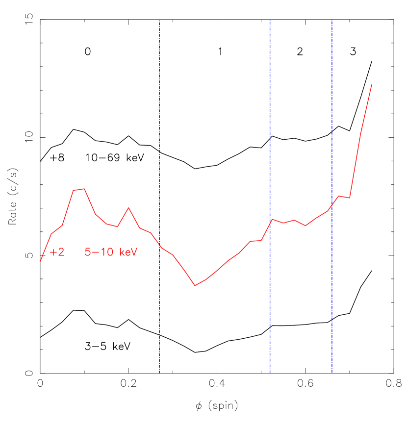
Figure 5: Average spin pulse, as a function of energy, folded over the $P_{\rm spin}=5750\pm 10$ s period. Offsets of $+2$ and $+8$ c s^-1 has been added, for the sake of clarity. Several flux levels of the source are separated by vertical lines. Note the similarity with the individual pulse in the inset of Fig. 1.

Both components are modified at low energies by photoelectric absorption which accounts for the local and interstellar material. The photoelectric absorption has been modeled using tbnew which contains the most up to date cross sections for X-ray absorption. Finally, a gaussian component has been added to describe the Fe K$\alpha$ fluorescence line. The best fit parameters are presented in Table 3. The norm of the additional blackbody is 5 orders of magnitude lower than the compmag component. In any case, it has no impact on the high energies we are focused in, and we do not discuss it further.

In agreement with previous studies, the temperature of the soft photon source is quite high $kT_{\rm bb}\simeq 1.5$ keV. At a distance of $d=3.7\pm 0.4$ kpc (Gaia Collaboration et al., 2016; Luri et al., 2018) the 0.3–20 keV luminosity would be in the range $L_{\rm X}=[4.7-11]\times 10^{35}$ erg s^-1 for spin phases 1 (low flux) and 3 (high flux), respectively ($6.5\times 10^{35}$ erg s^-1 average), roughly one order of magnitude lower than those usually found in HMXBs. This is consistent with a small emission area, presumably a hot spot on the NS surface (Torrejón et al., 2004). The conclusion is further supported by the NuSTAR analysis. Indeed, $r_{0}$ is the accretion column radius, in units of the NS Schwarzschild radius, or $r_{0}\simeq 0.84$ km. On the other hand, from the normalization constant $(R_{\rm km}/d_{10\rm kpc})^{2}$ a soft photons source radius of $R_{\rm km}=1.7$ km is derived. Finally, the albedo, $0<A<1$, is consistent with reflection from a NS surface .

Table 3: Model compmag+bb continuum parameters. Uncertainties are given at 90% confindence level.

Parameter	$\phi_{\rm spin}=0$	1	2	3	average
		COMPMAG
$N_{\rm H,1}$ (1022 cm-2)	0.8${}^{+0.3}_{-0.3}$	0.9${}^{+0.4}_{-0.4}$	0.83${}^{+0.15}_{-0.15}$	0.83${}^{+0.19}_{-0.19}$	0.83${}^{+0.09}_{-0.07}$
Norm	23.96${}^{+0.11}_{-0.31}$	15.58${}^{+0.06}_{-0.06}$	25.03${}^{+0.11}_{-0.09}$	34.88${}^{+0.13}_{-0.13}$	20.98${}^{+0.04}_{-0.04}$
$kT_{\rm bb}$ (keV)	1.54${}^{+0.04}_{-0.04}$	1.54${}^{+0.01}_{-0.01}$	1.543${}^{+0.002}_{-0.002}$	1.544${}^{+0.002}_{-0.002}$	1.557${}^{+0.001}_{-0.001}$
$kT_{\rm e}$ (keV)	16.0${}^{+0.4}_{-0.5}$	15.9${}^{+0.6}_{-0.6}$	17.00${}^{+0.03}_{-0.24}$	16.78${}^{+0.21}_{-0.21}$	16.01${}^{+0.11}_{-0.10}$
$\tau$	0.23${}^{+0.11}_{-0.11}$	0.23${}^{+0.10}_{-0.10}$	0.225${}^{+0.001}_{-0.001}$	0.222${}^{+0.002}_{-0.002}$	0.226${}^{+0.001}_{-0.001}$
$\beta_{0}$	0.08${}^{+0.09}_{-0.09}$	0.13${}^{+0.07}_{-0.07}$	0.127${}^{+0.002}_{-0.002}$	0.127${}^{+0.017}_{-0.015}$	0.081${}^{+0.011}_{-0.011}$
$r_{\rm 0}$	0.2${}^{+0.1}_{-0.1}$	0.2${}^{+0.1}_{-0.2}$	0.195${}^{+0.002}_{-0.001}$	0.198${}^{+0.001}_{-0.001}$	0.200${}^{+0.001}_{-0.001}$
$A$	0.5${}^{+0.3}_{-0.3}$	0.5${}^{+0.3}_{-0.3}$	0.61${}^{+0.02}_{-0.01}$	0.66${}^{+0.02}_{-0.02}$	0.57${}^{+0.01}_{-0.01}$
Fluxa	$4.49^{+0.01}_{-0.01}$	$2.86^{+0.01}_{-0.01}$	$4.73^{+0.02}_{-0.02}$	$6.61^{+0.02}_{-0.02}$	$3.94^{+0.09}_{-0.09}$
		BB
Norm (10-4)	5.4${}^{+0.3}_{-0.3}$	3.30${}^{+0.12}_{-0.12}$	5.8${}^{+0.3}_{-0.2}$	7.1${}^{+0.4}_{-0.4}$	4.77${}^{+0.11}_{-0.11}$
$kT$ (keV)	0.75${}^{+0.27}_{-0.17}$	0.75${}^{+0.13}_{-0.17}$	0.62${}^{+0.01}_{-0.01}$	0.61${}^{+0.01}_{-0.01}$	0.69${}^{+0.01}_{-0.01}$
Fluxa	0.28${}^{+0.02}_{-0.02}$	0.17 ${}^{+0.01}_{-0.01}$	0.24 ${}^{+0.01}_{-0.01}$	0.28${}^{+0.02}_{-0.02}$	0.23${}^{+0.01}_{-0.01}$
		GAUSS
$E$ (keV)	6.42${}^{+0.10}_{-0.10}$	6.42${}^{+0.18}_{-0.06}$	6.42${}^{+0.13}_{-0.13}$	6.42${}^{+0.29}_{-0.29}$	6.42${}^{+0.08}_{-0.06}$
Flux ($\times 10^{-6}$ ph s-1 cm-2)	40${}^{+42}_{-24}$	43${}^{+17}_{-20}$	23${}^{+26}_{-23}$	29${}^{+37}_{-30}$	46${}^{+23}_{-23}$
$EW$ (eV)	4.3${}^{+4.3}_{-2.4}$	7.6${}^{+3.1}_{-2.4}$	2.5${}^{+2.8}_{-2.5}$	2.5${}^{+2.8}_{-2.3}$	5.91${}^{+3.11}_{-3.11}$
$\chi^{2}_{\rm r}$(d.o.f.)	1.02(522)	0.82(510)	1.14(532)	1.04(529)	0.98(745)

• Unabsorbed $2-65$ keV flux $\times 10^{-10}$ erg s^-1 cm^-2

• $\beta$ flag and $\eta$ fixed to 1

• $\sigma_{\rm Fe}$ fixed to 0.12 keV

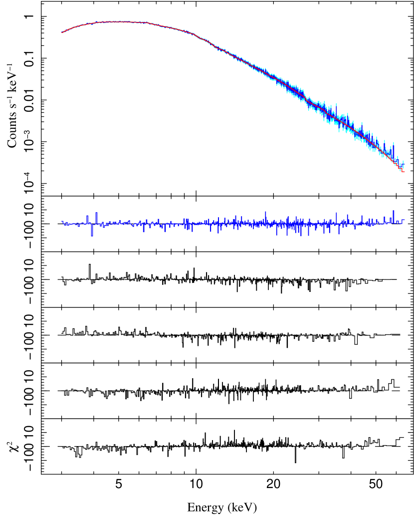
Figure 6: NuSTAR average spectrum (blue line) and best fit model (red line). The spectral models are described in detail in Section 4 and parameters given in Table 3. The residuals correspond to average (top) and spin phases 0, 1, 2 and 3, respectively.

4.1 No CRSF at 30 keV

The contiuum described above fits the NuSTAR spectra of 4U2206$+$54 perfectly in the high energy range. In Fig. 6 we show the phase averaged spectrum, the best model and the corresponding residuals. The region 20-40 keV does not show any peculiar residuals and does not require the addition of the previously claimed cyclotron line at $E_{\rm cyc}\sim 29$ keV. In order to search for any possible dependence on source brightness, we plot also the residuals of each individual spin phase, to the average model, renormalised. The spectrum shows little variability across the spin pulse. Likewise, no cyclotron line is detected in any of the spin phases.

In Table 4 we compile the cyclotron line (C.L.) claims along with the corresponding average source flux. The line is only detected in some observations but, again, there seems to be no correlation with the source flux in the long term. This casts serious doubts on the existence of the line. Thus, we can safely rule out the presence of any cyclotron line up to 60 keV.

Table 4: 4U2206+54 observations.

Instrument	Year	$F_{2-10}$a	C.L.	Ref.
RXTE	1997	2.5	N	1
Beppo SAX	1998	0.4	Y	1
RXTE	2001	1	Y	1
INTEGRAL (Rev. 67)	2003	15.9b	Y	2
INTEGRAL (Rev. 87)	2003	6.3	Y	2
RXTE	2007	2.5	N	3
XMM + INTEGRAL	2011	3.5	N	4
NuSTAR	2016	4	N	5

• Unabsorbed $2-10$ keV in units of $10^{-10}$ erg s^-1 cm^-2.

• 4- 150 keV

• Torrejón et al. (2004)

• Blay et al. (2005)

• Reig et al. (2009)

• Reig et al. (2012)

• This work

5 Discussion

The spin period of 4U2206$+$54 is rapidly decaying at a very high rate of $\dot{\nu}=-1.8\times 10^{-14}$ Hz s^-1. This suggests a strong negative torque applied to the magnetosphere of a slowly rotating neutron star. Under the assumption of a normal field strength ($B\sim 10^{12}$ G) the magnetic accretion model (Ikhsanov & Beskrovnaya, 2013) is able to explain the observed $\dot{\nu}$ provided that a) the stellar wind of the donor star presents some level of magnetization ($B>70$ G) and b) a dense magnetic slab of ambient matter forms around the magnetosphere of the NS. This disk like structure requires very special conditions to form in a wind fed system and the model parameters have to be within certain narrow ranges (see Ikhsanov & Beskrovnaya, 2013, for details).

Alternatively, such a torque can arise at the stage of subsonic settling accretion (Shakura et al., 2012) in a wind-fed X-ray binary, when a hot convective shell forms above the slowly rotating magnetosphere. The settling accretion requires an X-ray pulsar luminosity, $L_{\rm x}$, below a critical value of $\sim 4\times 10^{36}$ erg s^-1, which is the case for 4U 2206+54. The torque is caused by turbulent viscosity in the shell and can be negative if the X-ray luminosity drops down below the equilibrium value, $L_{\rm eq}$, determined by the balance between the angular momentum supply to, and removal from, the magnetosphere (see Shakura et al., 2012, for more detail and relevant formulas). The equilibrium luminosity depends on the NS magnetic dipole moment $\mu$ (the NS surface magnetic field $B=2\mu/R^{3}$, where $R$ is the NS radius), the binary orbital period $P_{\rm orb}$, the pulsar spin period $P_{*}$ and on the stellar wind velocity $v_{\rm w}$. In the case of 4U 2206+54, two possible binary orbital periods have been proposed 9.5 d (Ribó et al., 2006) and 19 d (Corbet et al., 2007). On the other hand, the magnetic field of the NS is unknown but the observed strong spin-down suggests the pulsar is not in equilibrium. Therefore, it is incorrect to use the equilibrium formulas to evaluate the NS magnetic moment. However, at X-ray luminosities much smaller than the equilibrium value, at the spin-down stage, it is still possible to obtain the lower limit of the NS dipole magnetic moment by neglecting the spin-up torque, which is independent of the stellar wind velocity and orbital binary period (see formulas in Shakura & Postnov, 2017):

$$\begin{matrix}\mu\geq\mu^{\prime\prime}\approx 1.7\times 10^{30}[\mathrm{G\,cm}^{3}]\Pi^{\prime\prime}\left|\frac{2\piup\dot{\nu}}{10^{-12}\mathrm{Hz\,s}^{-1}}\right|^{11/13}\\ \left(\frac{L_{x}}{10^{36}\mathrm{erg\,s}^{-1}}\right)^{-3/13}\left(\frac{P*}{100\mathrm{\,s}}\right)^{11/13}\end{matrix}$$ (1)

where $\Pi^{\prime\prime}\gtrsim 1$ is a combination of the dimensionless theory parameters. For 4U2206+54 we thus obtain $\mu>10^{31}$ G cm³, corresponding to the NS surface magnetic field $B_{\rm s}>2\times 10^{13}$ G. On the other hand, another estimate can be made if the orbital binary period $P_{\rm orb}$ and stellar wind velocity $v_{w}$ are used:

$$\begin{matrix}\mu\geq\mu^{\prime}\approx 0.94\times 10^{30}[\mathrm{G\,cm}^{3}]\Pi^{\prime}\left|\frac{2\piup\dot{\nu}}{10^{-12}\mathrm{Hz\,s}^{-1}}\right|^{1/2}\\ \left(\frac{v_{w}}{1000\mathrm{km\,s}^{-1}}\right)^{-3/2}\left(\frac{P*}{100\mathrm{\,s}}\right)^{7/8}\left(\frac{P_{\rm orb}}{10\mathrm{\,d}}\right)^{-3/8}\end{matrix}$$ (2)

Here $\Pi^{\prime}\gtrsim 1$ is another combination of dimensionless theory parameters. Note that this estimate does not depend on the NS X-ray luminosity because it is derived under the assumption that the observed $\dot{\nu}$ corresponds to the maximum possible spin-down rate of a NS at the settling accretion stage. Assuming $P_{\rm orb}=9.5$ d (Stoyanov et al., 2014), and using $v_{w}=350$ km s^-1 (Ribó et al., 2006), we obtain $\mu>2\times 10^{32}$ G cm³, which corresponds to a surface magnetic field $B_{\rm s}>2\times 10^{14}$ G. From both calculations, we can estimate a lower limit for the surface field strength $B_{\rm s}$ of several times $10^{13}$ G. The lack of a CRSF detection with NuSTAR would be consistent with this scenario. This value is in the vicinity of the quantum critical field $B_{\rm cr}=4.4\times 10^{13}$ G, which traditionally has been used to delimit the high end of the magnetic field distribution for pulsars from magnetars (Olausen & Kaspi, 2014, Fig. 7). Thus, among the wind accretion powered X-ray pulsars, 4U2206$+$54 would harbour a very high magnetic field NS.

6 Conclusions

From our analysis, the following conclusions can be drawn:

• NuSTAR spectra rule out any cyclotron line up to 60 keV.

• The secular strong spin down of 4U2206$+$54 is confirmed, at a rate of $\dot{\nu}=-1.8\times 10^{-14}$ Hz s^-1

• Under the spherical settling accretion scenario, the required surface magnetic field needs to be, at least, several times $10^{13}$ G, at the high end of the magnetic field distribution for pulsars. Thus, 4U2206$+$54 appears as a strongly magnetized NS, whose X-ray emission is powered by the accretion of the slow wind of its main sequence (O9.5V).

References

- Blay et al. (2005) Blay P., Ribó M., Negueruela I., Torrejón J. M., Reig P., Camero A., Mirabel I. F., Reglero V., 2005, A&A, 438, 963
- Chini et al. (2012) Chini R., Hoffmeister V. H., Nasseri A., Stahl O., Zinnecker H., 2012, MNRAS, 424, 1925
- Corbet et al. (2007) Corbet R. H. D., Markwardt C. B., Tueller J., 2007, ApJ, 655, 458
- Cumming et al. (1999) Cumming A., Marcy G. W., Butler R. P., 1999, ApJ, 526, 890
- Farinelli et al. (2012) Farinelli R., Ceccobello C., Romano P., Titarchuk L., 2012, A&A, 538, A67
- Finger et al. (2010) Finger M. H., Ikhsanov N. R., Wilson-Hodge C. A., Patel S. K., 2010, ApJ, 709, 1249
- Gaia Collaboration et al. (2016) Gaia Collaboration et al., 2016, A&A, 595, A1
- Hickox et al. (2004) Hickox R. C., Narayan R., Kallman T. R., 2004, ApJ, 614, 881
- Houck & Denicola (2000) Houck J. C., Denicola L. A., 2000, in Manset N., Veillet C., Crabtree D., eds, Astronomical Society of the Pacific Conference Series Vol. 216, Astronomical Data Analysis Software and Systems IX. p. 591
- Ikhsanov & Beskrovnaya (2010) Ikhsanov N. R., Beskrovnaya N. G., 2010, Astrophysics, 53, 237
- Ikhsanov & Beskrovnaya (2013) Ikhsanov N. R., Beskrovnaya N. G., 2013, Astronomy Reports, 57, 287
- Liu et al. (2006) Liu Q. Z., van Paradijs J., van den Heuvel E. P. J., 2006, A&A, 455, 1165
- Lomb (1976) Lomb N. R., 1976, Ap&SS, 39, 447
- Luri et al. (2018) Luri X., et al., 2018, preprint, (arXiv:1804.09376)
- Olausen & Kaspi (2014) Olausen S. A., Kaspi V. M., 2014, ApJS, 212, 6
- Postnov & Yungelson (2014) Postnov K. A., Yungelson L. R., 2014, Living Reviews in Relativity, 17, 3
- Press & Rybicki (1989) Press W. H., Rybicki G. B., 1989, ApJ, 338, 277
- Reig et al. (2009) Reig P., Torrejón J. M., Negueruela I., Blay P., Ribó M., Wilms J., 2009, A&A, 494, 1073
- Reig et al. (2012) Reig P., Torrejón J. M., Blay P., 2012, MNRAS, 425, 595
- Ribó et al. (2006) Ribó M., Negueruela I., Blay P., Torrejón J. M., Reig P., 2006, A&A, 449, 687
- Roberts et al. (1987) Roberts D. H., Lehar J., Dreher J. W., 1987, AJ, 93, 968
- Sana et al. (2012) Sana H., et al., 2012, Science, 337, 444
- Sanjurjo-Ferrrín et al. (2017) Sanjurjo-Ferrrín G., Torrejón J. M., Postnov K., Oskinova L., Rodes-Roca J. J., Bernabeu G., 2017, A&A, 606, A145
- Scargle (1982) Scargle J. D., 1982, ApJ, 263, 835
- Shakura & Postnov (2017) Shakura N., Postnov K., 2017, preprint, (arXiv:1702.03393)
- Shakura et al. (2012) Shakura N., Postnov K., Kochetkova A., Hjalmarsdotter L., 2012, MNRAS, 420, 216
- Sidoli et al. (2017) Sidoli L., Israel G. L., Esposito P., Rodríguez Castillo G. A., Postnov K., 2017, MNRAS, 469, 3056
- Stellingwerf (1978) Stellingwerf R. F., 1978, ApJ, 224, 953
- Stoyanov et al. (2014) Stoyanov K. A., Zamanov R. K., Latev G. Y., Abedin A. Y., Tomov N. A., 2014, Astronomische Nachrichten, 335, 1060
- Thompson & Beloborodov (2005) Thompson C., Beloborodov A. M., 2005, ApJ, 634, 565
- Thompson & Duncan (1993) Thompson C., Duncan R. C., 1993, ApJ, 408, 194
- Thompson et al. (2002) Thompson C., Lyutikov M., Kulkarni S. R., 2002, ApJ, 574, 332
- Torrejón et al. (2004) Torrejón J. M., Kreykenbohm I., Orr A., Titarchuk L., Negueruela I., 2004, A&A, 423, 301
- Townsend (2010) Townsend R. H. D., 2010, ApJS, 191, 247
- VanderPlas (2017) VanderPlas J. T., 2017, preprint, (arXiv:1703.09824)
- Walton et al. (2016) Walton D. J., et al., 2016, ApJ, 826, 87
- Wang (2009) Wang W., 2009, MNRAS, 398, 1428
- Woods & Thompson (2006) Woods P. M., Thompson C., 2006, Soft gamma repeaters and anomalous X-ray pulsars: magnetar candidates. pp 547–586
- Zechmeister & Kürster (2009) Zechmeister M., Kürster M., 2009, A&A, 496, 577
- van den Heuvel & De Loore (1973) van den Heuvel E. P. J., De Loore C., 1973, A&A, 25, 387