End-to-End Neural Ranking for eCommerce Product Search

Abstract.

We consider the problem of retrieving and ranking items in an eCommerce catalog, often called SKUs, in order of relevance to a user-issued query. The input data for the ranking are the texts of the queries and textual fields of the SKUs indexed in the catalog. We review the ways in which this problem both resembles and differs from the problems of information retrieval (IR) in the context of web search, which is the context typically assumed in the IR literature. The differences between the product-search problem and the IR problem of web search necessitate a different approach in terms of both models and datasets. We first review the recent state-of-the-art models for web search IR, focusing on the CLSM of (Shen et al., 2014) as a representative of one type, which we call the distributed type, and the kernel pooling model of (Xiong et al., 2017), as a representative of another type, which we call the local-interaction type. The different types of relevance models developed for IR have complementary advantages and disadvantages when applied to eCommerce product search. Further, we explain why the conventional methods for dataset construction employed in the IR literature fail to produce data which suffices for training or evaluation of models for eCommerce product search. We explain how our own approach, applying task modeling techniques to the click-through logs of an eCommerce site, enables the construction of a large-scale dataset for training and robust benchmarking of relevance models. Our experiments consist of applying several of the models from the IR literature to our own dataset. Empirically, we have established that, when applied to our dataset, certain models of local-interaction type reduce ranking errors by one-third compared to the baseline system (tf—idf). Applied to our dataset, the distributed models fail to outperform the baseline. As a basis for a deployed system, the distributed models have several advantages, computationally, over the local-interaction models. This motivates an ongoing program of work, which we outline at the conclusion of the paper.

1. Introduction

Currently deployed systems for eCommerce product search tend to use inverted-index based retrieval, as implemented in Elasticsearch (Gormley and Tong, 2015) or Solr (Smiley et al., 2015). For ranking, these systems typically use legacy relevance functions such as tf—idf (Wikipedia, 2018) or Okpai BM25 (Robertson et al., 2009), as implemented in these search systems. Such relevance functions are based on exact (”hard”) matches of tokens, rather than semantic (”soft”) matches, are insensitive to word order, and have hard-coded, rather than learned weights. On the one hand, their simplicity makes legacy relevance functions scalable and easy-to-implement. One the other hand, they are found to be inadequate in practice for fine-grained ranking of search results. Typically, in order to achieve rankings of search results that are acceptable for presentation to the user, eCommerce sites overlay on top of the legacy relevance function score, a variety of handcrafted filters (using structured data fields) as well as hard-coded rules for specific queries. In some cases, eCommerce sites are able to develop intricate and specialized proprietary NLP systems, referred to as Query-SKU Understanding (QSU) Systems, for analyzing and matching relevant SKUs to queries. QSU systems, while potentially very effective at addressing the shortcomings of legacy relevance scores, require a some degree of domain-specific knowledge to engineer (Kutiyanawala et al., 2018). Because of concept drift, the maintenance of QSU systems demands a long-term commitment of analyst and programmer labor. As a result of these scalability issues, QSU systems are within reach only for the very largest eCommerce companies with abundant resources.

Recently, the field of neural IR (NIR) , has shown great promise to overturn this state of affairs. The approach of NIR to ranking differs from the aforementioned QSU systems in that it learns vector-space representations of both queries and SKUs which facilitate learning-to-rank (LTR) models to address the task of relevance ranking in an end-to-end manner. NIR, if successfully applied to eCommerce, can allow any company with access to commodity GPUs and abunant user click-through logs to build an accurate and robust model for ranking search results at lower cost over the long-term compared to a QSU system. For a current and comprehensive review of the field of NIR, see (Mitra and Craswell, 2017).

Our aim in this paper is to provide further theoretical justification and empirical evidence that fresh ideas and techniques are needed to make Neural IR a practical alternative to legacy relevance and rule-based systems for eCommerce search. Based on the results of model training which we present, we delineate a handful of ideas which appear promising so far and deserve further development.

2. Relation to Previous Work in Neural IR

The field of NIR shares its origin with the more general field of neural NLP (Goldberg, 2017) in the word embeddings work of word2vec (Le and Mikolov, 2014) and its variants. From there, though, the field diverges from the more general stream of neural NLP in a variety of ways. The task of NIR, as compared with other widely known branches such as topic modeling, document clustering, machine translation and automatic summarization, consists of matching texts from one collection (the queries) with texts from another collection (webpages or SKUs, or other corpus entries, as the case may be). The specific challenges and innovations of NIR in terms of models are driven by the fact that entries from the two collections (queries versus documents) are of a very different nature from one another, both in length, and internal structure and semantics.

In terms of datasets, the notion of relevance has to be defined in relation to a specific IR task and the population which will use the system. In contrast to the way many general NLP models can be trained and evaluated on publicly available labeled benchmark corpora, a NIR model has to be trained on a datasest tailored to reflect the information needs of of the population the system is meant to serve. In order to produce such task-specific datasets in a reliable and scalable manner, practitioners need to go beyond traditional methods such as expert labeling and simple statistical aggregations. The solution has been to take ”crowdsourcing” to its logical conclusion and to use the ”big data” of user logs to extract relevance judgments. This has led NIR to depend for scalability on the field of Click Models, which are discussed at great length in the context of web search in the book (Chuklin et al., 2015).

While NIR has great promise for application to eCommerce, the existing NIR literature has thus far been biased towards the web search problem, relegating eCommerce product search to ”niche” field status. We hope to remedy this situation by demonstrating the need for radical innovation in the field of NIR to address the challenges of eCommerce product search.

One of the most important differences is that for product search, as compared to web search, both the intent and vocabulary of queries tend to be more restricted and ”predictable”. For example, when typing into a commercial web search engine, people can be expected to search for any type of information. Generally speaking, customers on a particular eCommerce site are only looking to satisfy only one type of information need, namely to retrieve a list of SKUs in the catalog meeting certain criteria. Users, both customers and merchants, are highly motivated by economic concerns (time and money spent) to craft queries and SKU text fields to facilitate the surfacing of relevant content, for example, by training themselves to pack popular and descriptive keywords into queries and SKUs. As a consequence, the non-neural baselines, such as tf—idf, tend to achieve higher scores on IR metrics in product search datasets than in web search. An NIR model, when applied to product search as opposed to web search, has a higher bar to clear to justify the added system complexity.

Further, the lift NIR provides over tf—idf is largely in detecting semantic, non-exact matches. For example, consider a user searching the web with the query ”king’s castle”. This user will likely have her information need met with a document about the ”monarch’s castle” or even possibly ”queen’s castle”, even if it does not explicitly mention ”king”. In contrast, consider the user issuing the query ”king bed” on an eCommerce site. She would likely consider a ”Monarch bed” irrelevant unless that bed is also ”king”, and a ”queen bed” even more irrelevant. An approach based on word2vec or Glove (Pennington et al., 2014) vectors would likely consider the words ”king”, ”queen” and ”monarch” all similar to one another based on the distributional hypothesis. The baseline systems deployed on eCommerce websites often deal with semantic similarity by incorporating analyzers with handcrafted synonym lists built in, an approach which is completely infeasible for open-domain web search. This further blunts the positive impact of learned semantic similarity relationships.

Another difference between ”general” IR for web-search and IR specialized for eCommerce product search is that in the latter the relevance landscape is simutaneously ”flatter” and more ”jagged”. With regard to ”flatness”, consider a very popular web search for 2017 (according to (Trends, 2018)): ”how to make solar eclipse glasses”. Although the query expresses a very specific search intent, it is likely that the user making it has other, related information needs. Consequently, a good search engine results page (SERP), could be composed entirely of links to instructions on making solar eclipse glasses, which while completely relevant, could be redundant. A better SERP would be composed of a mixture of the former, and of links to retailers selling materials for making such glasses, to instructions on how to use the glasses, and to the best locations for viewing the upcoming eclipse, all which are likely relevant to some degree to the user’s infromation need and improve SERP diversity. In contrast, consider the situation for a more typical eCommerce query: ”tv remote”. A good product list view (PLV) page for the search ”tv remote” would display exclusively SKUs which are tv remotes, and no SKUs which are tvs. Further, all the ”tv remote” SKUs are equally relevant to the query, though some might be more popular and engaging than others. With regard to ”jaggedness”, consider the query ”desk chair”: any ”desk with chair” SKUs would be considered completely irrelevant and do not belong anywhere on the PLV page, spite of the very small lexical difference between the queries ”desk chair” and ”desk with chair”. In web search, by contrast, documents which are relevant for a given query tend to remain partially relevant for queries which are lexically similar to the original query. If the NIR system is to compete with currently deployed rule-based systems, it is of great importance for a dataset for training and benchmarking NIR models for product search to incorporate such ”adversarial” examples prevalently.

Complications arise when we estimate relevance from the click-through logs of an eCommerce site, as compared to web search logs. Price, image quality are factors comparable in importance to relevance in driving customer click behavior. As an illustration, consider the situation in which the top-ranked result on a SERP or PLV page for a query has a lower click-through rate (CTR) than the documents or SKUs at lower ranks. In the web SERP case, the low CTR sends a strong signal that the document is irrelevant to the query, but in the eCommerce PLV it may have other other explanations, for example, the SKU’s being mispriced or having an inferior brand or image. We will address this point in much more detail in Section 4 below.

Another factor which assumes more importance in the field of eCommerce search versus web search is the difference between using the NIR model for ranking only and using it for retrieval and ranking. In the former scenario, the model is applied at runtime as the last step of a pipeline or ”cascade”, where earlier steps of the pipeline use cruder but computationally faster techniques (such as inverted indexes and tf—idf) to identify a small subcorpus (of say a few hundred SKUs) as potential entries on the PLV page, and the NIR model only re-ranks this subcorpus (see e.g. (Tu et al., 2017)). In the latter scenario, the model, or more precisely, approximate nearest neighbor (ANN) methods acting on vector representations derived from the model, both select and rank the search results for the PLV page from the entire corpus. The latter scenario, retrieval and ranking as one step, is more desirable but (see §§3 and 6 below) poses additional challenges for both algorithm developers and engineers. The possibility of using the NIR model for retrieval, as opposed to mere re-ranking, receives relatively little attention in the web search literature, presumably because of its infeasibility: the corpus of web documents is so vast, in the trillions (Venturebeat.com, 2013), compared to only a few million items in each category of eCommerce SKUs.

3. Neural Information Retrieval Models

In terms of the high-level classification of Machine Learning tasks, which includes such categories as ”classification” and ”regression”, Neural Information Retrieval (NIR) falls under the Learning to Rank (LTR) category (see (Li, 2014) for a comprehensive survey). An LTR algorithm uses an objective function defined over possible ”queries” $q\in Q$ and lists of ”documents” $d\in D$, to learn a model that, when applied to an new previously unseen query, uses the features of the both the query and documents to ”optimally” order the documents for that query. For a more formal definition, see §1.3 of (Li, 2014). As explained in §2.3.2 of (Li, 2014), it is common practice in IR to approximate the general LTR task with a binary classification task. For the sake of simplicity, we follow this so-called ”pairwise approach” to LTR. Namely, we first consider LTR algorithms whose orderings are induced from a scoring function $f:Q\times D\rightarrow\mathbf{R}$ in the sense that the ordering for $q$ consists of sorting $D$ in the order $d_{1},\ldots d_{N}$ satisfying $f(q,d_{1})\geq f(q,d_{2})\geq\cdots f(q,d_{N})$. Next, we train and evaluate the LTR model by presenting it with triples $(q,d_{\rm rel},d_{\rm irrel})\in Q\times D\times D$, where $d_{\rm rel}$ is deemed to be more relevant to $q$ than $d_{\rm irrel}$: the binary classification task amounts to assigning scores $f$ so that $f(q,d_{\rm rel})>f(q,d_{\rm irrel})$.

There are many ways of classifying the popular types of NIR models, but the way that we find most fundamental and useful for our purposes is the classification into distributed and local-interaction models. The distinction between the two types of models lies in the following architectural difference. The first type of model first transforms $d$ and $q$ into ”distributed” vector representations $v_{D}(d)\in V_{D}$ and $v_{Q}(q)\in V_{Q}$ of fixed dimension, and only after that feeds the representations into an LTR model. The second type of model never forms a fixed-dimensional ”distributed” vector representation of document or query, and instead forms a ”interaction” matrix representation $\langle i(q),i(d)\rangle$ of the pair $(q,d)$. The matrix $\langle i(q),i(d)\rangle$ is sensitive only to local, not global, interactions between $q$ and $d$, and the model subsequently uses $\langle i(q),i(d)\rangle$ as the input to the LTR model. More formally, in the notation of Table 1, the score function $f$ takes the following form in the distributed case:

(1) $$f(q,d)=r\left(v_{Q}(q),v_{D}(d)\right)=r\left(g_{Q}(i(q)),g_{D}(i(d))\right),$$

and the following form in the local-interaction case:

(2) $$f(q,d)=r\big{(}\langle i(q),i(d)\rangle\big{)}.$$

Thus, the interaction between $q$ and $d$ occurs at a global level in the distributed case and at the local level in the local-interaction case. The NIR models are distinguished individually from others of the same type by the choices of building blocks in Table 1. In Tables 2 and 3, we show how to obtain some common NIR models in the literature by making specific choices of the building blocks. Note that since $w$ determines $i$, and $g,i$ together determine $v$, to specify a local-interaction model (Table 3) we only need to specify the mappings $w,r$, and to specify a distributed NIR model (Table 2), we need only additionally specify $g$. We remark that the distributed word embeddings in the ”Siamese” and Kernel Pooling models are implicitly assumed to be normalized to have $2$-norm one, which allows the application the dot product $\langle\cdot,\cdot\rangle$ to compute the cosine similarity.

The classification of NIR models in Tables 2 and 3 is not meant to be an exhaustive list of all models found in the literature: for a more comprehensive exposition, see for example the baselines section §4.3 of (Xiong et al., 2017). Laying out the models in this fashion facilitates a determination of which parts of the ”space” of possible models remain unexplored. For example, we see the possibility of forming a new ”hybrid” by using the distributed word embeddings layer $w$ from the Kernel Pooling model (Xiong et al., 2017), followed by the representation layer $g$ from CLSM (Shen et al., 2014), and we have called this distributed model, apparently nowhere considered in the existing literature ”Siamese”. Substituting into (1), we obtain the following formula for the score $f$ of the Siamese model:

(3) $$f(q,d)=\langle\mathrm{mlp}_{1}\circ\mathrm{cnn}_{1}(i(q)),\mathrm{mlp}_{1}\circ\mathrm{cnn}_{1}(i(d))\rangle.$$

As an example missing from the space of possible local-interaction models, we have not seen any consideration of the ”hybrid” architecture obtained by using the local-interaction layer from the Kernel-Pooling model and a position-aware LTR layer such as a convolution neural net. Substituting into (2), the score function would be

(4) $$f(q,d)=\mathrm{mlp}\circ\mathrm{cnn}\big{(}\langle i(q),i(d)\rangle\big{)},$$

where in both (3) and (4), $i$ is the embedding layer obtained induced by a trainable word embedding $w$. These are just a couple of the other new architectures which could be formed in this way: we just highlight these two because they seem especially promising.

The main benefit of distinguishing between distributed and local-interaction models is that a distributed architecture enables retrieval-and-ranking, whereas a local-interaction architecture restricts the model to re-ranking the results of a separate retrieval mechanism. See the last paragraph of Section 2 for an explanation of this distinction. From a computational complexity perspective, the reason for this is that the task of precomputing and storing all the representations involved in computing the score is, for a distributed model, $O(|Q|+|D|)$ in space and time, but for a local-interaction model, $O(|Q||D|)$. (Note that we need to compute the representations which are the inputs to $r$, namely, in the distributed case, the vectors $v_{Q}(q)$, $v_{D}(d)$, and in the local-interaction case, the matrices $\langle i(q),i(d)\rangle$: computing the variable-length representations $i(d)$ and $i(q)$ alone will not suffice in either case). Further, in the distributed model case, assuming the LTR function $r(\cdot)$ is chosen to be the dot-product $\langle\cdot,\cdot\rangle$, the retrieval step can be implemented by ANN. This is the reason for the choice of $r$ as $\langle\cdot,\cdot\rangle$ in defining the ”Siamese” model. For practical implementations of ANN using Elasticsearch at industrial scale, see (Rygl et al., 2017) for a general text-data use-case, and (Mu et al., 2018) for an image-data use-case in an e-Commerce context. We will return to this point in §7.

Table 1. Notation for Building Blocks of NIR models

Symbol	Meaning	Examples or Formulas
$\langle\cdot,\cdot\rangle$	dot-product $\langle A,B\rangle=A\cdot B^{T}$ for vectors or matrices $A,B$	$A\in\mathbf{R}^{m\times k},B\in\mathbf{R}^{n\times k}\Rightarrow\langle A,B\rangle\in\mathbf{R}^{m\times n}$, $\langle A,B\rangle_{i,j}=\sum_{\ell=1}^{k}A_{i,\ell}B_{j,\ell}$
$[\ldots]$	Matrix Augmentation (concatenation)	$A_{1},\ldots,A_{K}\in\mathbf{R}^{M\times N}\Rightarrow[A_{1},\ldots,A_{k}]\in\mathbf{R}^{M\times KN}$
$\mathrm{mlp}_{k}$	fully-connected ($k$-layer) perceptron	$\mathrm{mlp}_{2}(x)=\tanh(W_{2}\cdot\tanh(W_{1}\cdot x+b_{1})+b_{2})$, $W_{i}$ weight matrices
$\mathrm{cnn}_{k}$	$k$-layer convolutional nn (with possible max-pooling)	$\mathrm{cnn}_{1}(x)=\tanh(W_{c}\cdot x)$, $W_{c}$ convolutional weight matrix
$w$	word or embedding	word hashing of (Huang et al., 2013) mapping derived from word2vec, e.g. token $t\mapsto w(t)\in\mathbf{R}^{300}$
$i$	local document embedding	$i:[t_{1},\ldots,t_{k}]\mapsto[\underbrace{w(t_{1})^{T},\ldots,w(t_{k}^{\prime})^{T}}_{k^{\prime}=\min(k,N)},\underbrace{\mathbf{0}^{T},\ldots,\mathbf{0}^{T}}_{N-k^{\prime}\;\mathrm{times}}]\in\mathbf{R}^{300\times N}$
$N_{\{Q|D\}}$	Dimension of local document embedding along token axis	$N_{D}=1000$, $N_{Q}=10$ for Duet model.
$V_{\{Q|D\}}$	Vector space for distributed representations of $D$ or $Q$	$V_{Q}=\mathbf{R}^{300}$, $V_{D}=\mathbf{R}^{300\times 899}$ for Duet Model
$V$	Vector space for distributed representations of $D$ and $Q$	as above, when $V_{Q}=V_{D}$.
$g_{\{Q|D\}}$	parameterized mapping of $i(\{q|d\})$ to $v_{\{q|d\}}(\{q|d\})\in V_{\{Q|D\}}$	$\mathrm{mlp}$; $\mathrm{cnn}$; $\mathrm{mlp}\circ\mathrm{cnn}$; $\mathrm{mlp}\circ\sigma_{1}$
$g$	parameterized mapping of $i(d)$, $i(q)$ to $v\in V$	special case of above, when $V_{Q}=V_{D}$, and $g_{Q}=g_{D}$
$v_{\{Q|D\}}$	$g_{\{q|d\}}\circ i$, global document embedding of $q$ or $d$ into $V_{\{Q|D\}}$	composition or previous mappings
$v$	$g\circ i$, global document embedding of $q$ or $d$ into $V$	special case when $V_{Q}=V_{D}$, and $g_{Q}=g_{D}$, $v_{Q}=v_{D}$
$r$	LTR model mapping $\langle i(q),i(d)\rangle$ or $(v_{Q}(q),v_{D}(d))\mapsto\mathbf{R}$	$\langle\cdot,\cdot\rangle$ (Shen et al., 2014); $\mathrm{mlp}_{3}\circ\bigodot$ (Mitra et al., 2017); $\mathrm{mlp}_{1}\circ\mathbf{K}$ (Xiong et al., 2017)
$\sigma_{1}$	summation along $1$-axis, mapping $\mathbf{R}^{m\times n}\rightarrow\mathbf{R}^{m}$	$\sigma_{1}:\mathbf{R}^{m\times n}\rightarrow\mathbf{R}^{m}$, $\sigma_{1}(A)_{i}=\sum_{j=1}^{n}A_{i,j}$
$\bigodot$	Hadamard (elementwise) product (of matrices, tensors)	$A,B\in\mathbf{R}^{m\times n}\Rightarrow A\bigodot B\in\mathrm{R}^{m\times n}$
$\bigodot$	Broadcasting, followed by Hadamard (operator overloading)	$A\in R^{m},B\in R^{m\times n}\Rightarrow A\bigodot B=[\underbrace{A,\ldots,A}_{n\;\textbf{times}}]\bigodot B$
$\mathbf{K}$	Kernel-pooling map of (Xiong et al., 2017)	$\mathbf{K}(M_{i})=[K_{1},\ldots,K_{K}]$, $K_{k}$ RBF kernels with mean $\mu_{k}$.
$\phi$	Kernel-pooling composed with soft TF map of (Xiong et al., 2017)	$M\in\mathbf{R}^{N_{Q}\times N_{D}}\Rightarrow\phi(M)=\sum_{i=1}^{N_{Q}}\log\mathbf{K}(M_{i})$

Table 2. Comparison of distributed NIR models in literature

Model	$w$	$\mathrm{dim}(w)$	$g_{Q}$	$g_{D}$	$\mathrm{dim}\left(V_{Q}\right)$	$\mathrm{dim}\big{(}V_{D}\big{)}$	$r$
DSSM (Huang et al., 2013)	”word hashing”, see (Huang et al., 2013)	$30,000$	$\mathrm{mlp}_{3}\circ\sigma_{1}$	$=g_{Q}$	$128$	$128$	$\langle\cdot,\cdot\rangle$
CLSM (Shen et al., 2014)	”word hashing”, see (Huang et al., 2013)	$30,000$	$\mathrm{mlp}_{1}\circ\mathrm{cnn}_{1}$	$=g_{Q}$	$128$	$128$	$\langle\cdot,\cdot\rangle$
Duet (Mitra et al., 2017) (distributed side)	”word hashing”, see (Huang et al., 2013)	$2000$	$\mathrm{mlp}_{1}\circ\mathrm{cnn}_{1}$	$\mathrm{cnn}_{2}$	$300$	$300\times 899$	$\mathrm{mlp}_{3}\circ\bigodot$
”Siamese” (ours)	distributed word embeddings	$300$	$\mathrm{mlp}_{1}\circ\mathrm{cnn}_{1}$	$=g_{Q}$	$32-512$	$32-512$	$\langle\cdot,\cdot\rangle$

Table 3. Comparison of local-interaction NIR models in literature

Model	$w$	$\mathrm{dim}(w)$	$r$
tf—idf	one-hot encoding, weighted by $\sqrt{\mathrm{idf}}$	$|\mathrm{Vocabulary}|$	$\sigma_{1}:\,\mathbf{R}^{|\mathrm{Vocabulary}|}_{+}\rightarrow\mathbf{R}_{+}$
Duet (Mitra et al., 2017) (local side)	one-hot encoding	$|\mathrm{Vocabulary}|$	$\mathrm{mlp}_{3}\circ\mathrm{cnn}_{1}$
Kernel-pooling model (Xiong et al., 2017)	distributed word embeddings	$300$	$\mathrm{mlp}_{1}\circ\phi$

4. From Click Models to Task Models

4.1. Click Models

The purpose of click models is to extract, from observed variables, an estimate of latent variables. The observed variables generally include the sequence of queries, PLVs/SERPs and clicks, and may also include hovers, add-to-carts (ATCs), and other browser interactions recorded in the site’s web-logs. The main latent variables are the relevance and attractiveness of an item to a user. A click model historically takes the form of a probabilistic graphical model called a Bayesian Network (BN), whose structure is represented by a Directed Acyclic Graph (DAG), though more recent works have introduced other types of probabilistic model including recurrent (Borisov et al., 2016) and adversarial (Moore et al., 2018) neural networks. The click model embodies certain assumptions about how users behave on the site. We are going to focus on the commonalities of the various click models rather than their individual differences, because our aim in discussing them is to motivate another type of model called task models, which will be used to construct the experimental dataset in Section 4.

To model the stochasticity inherent in the user browsing process, click models adopt the machinery of probability theory and conceptualize the click event, as well as related events such as examinations, ATCs, etc., as the outcome of a (Bernoulli) random variable. The three fundamental events for describing user interaction with a SKU $u$ on a PLV are denoted as follows:

1. The user examining the SKU, denoted by $E_{u}$;

2. The user being sufficiently attracted by the SKU ”tile” to click it, denoted by $A_{u}$;

3. The user clicking on the SKU, by $C_{u}$.

The most basic assumption relating these three events is the following Examination Hypothesis (Equation (3.4), p. 10 of (Chuklin et al., 2015)):

(5) $$\text{{EH}}\quad C_{u}=1\Leftrightarrow E_{u}=1\;\text{and}\;A_{u}=1.$$

The EH is universally shared by click models, in view of the observation that any click which the user makes without examining the SKU is just ”noise” because it cannot convey any information about the SKU’s relevance. In addition, most of the standard click models, including the Position Based (PBM) and Cascade (CM) Models, also incorporate the following Independence Hypothesis:

(6) $$\textbf{{IH}}\quad E_{u}\,\raisebox{0.50003pt}{\rotatebox[origin={c}]{90.0}{$\models$}}\,A_{u}.$$

The IH appears reasonable because the attractiveness of a SKU represents an inherent property of the query-SKU pair, whereas whether the SKU is examined is an event contingent on a particular presentation on the PLV and the individual user’s behavior. This means that $E_{u}$ and $A_{u}$ should not be able to influence one another, as the IH claims. Adding the following two ingredients to the EH (5) and the IH (6), we obtain a functional, if minimal, click model

1. A probabilistic description of how the user interacts with the PLV: i.e., at a minimum, a probabilistic model of the variables $E_{u}$.

2. A parameterization of the distributions underlying the variables $A_{u}$.

We can specify a simple click model by carrying out (1)–(2) as follows:

1. $P(E_{u}=1)$ depends only on the rank of $u$, and is given by a single parameter $\gamma_{r}$ for each rank, so that $P(E_{u_{r}})=:\gamma_{r}\in[0,1]$.

2. $P(A_{u}=1|E_{u}=1)=:\alpha_{u,q}\in[0,1]$, where there is an independent Bernoulli parameter $\alpha_{u,q}$ for each pair of query and SKU.

The click model obtained by specifying (1)–(2) as above is called the PBM. For a template-based representation of the PBM, see Figure 1. For further detail on the PBM and other BN click models, see (Chuklin et al., 2015), and for interpretation of template-based representations of BNs see Chapter 6 of (Koller and Friedman, 2009).

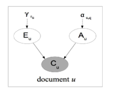
Figure 1. Template-based representation of the PBM click model.

The parameter estimation of click model BN’s relies on the following consequence of the EH (5):

(7) $$\left\{E_{u}=E_{u^{\prime}}=1\;\&\;\,C_{u}=0\;\&\;C_{u^{\prime}}=1\right\}\rightsquigarrow\alpha_{u^{\prime},q}>\alpha_{u,q},$$

where in (7), the symbol $\rightsquigarrow$ means ”increases the likelihood that”. This still leaves open the question of how to connect attractiveness to relevance, which click models need to do in order to fulfill their purpose, namely extracting relevance judgments from the click logs. The simplest way of making the connection is to assume that an item (web page or SKU) is attractive if and only if it is relevant, but this assumption is obviously implausible even in the web search case, and all but the simplest click models reject it. A more sophisticated approach, which is the option taken by click models such as DCM, CCD, DBN, is to define another Bernoulli random variable

1. $S_{u}$, the user having her information need satisfied by SKU $u$,

satisfying the following Click Hypothesis:

(8) $$\textbf{CH}\;C_{u}=0\Rightarrow S_{u}=0.$$

The CH is formally analogous to the EH, (5), since just as the EH says that only $u$ for which $E_{u}=1$ are eligible to have $C_{u}=1$, regardless of their inherent attractiveness $\alpha_{u,q}$, the CH says that only $u$ for which $C_{u}=1$ are eligible to have $S_{u}=1$, regardless of their inherent relevance $\sigma_{u,q}$. The justification of the CH is that the user cannot know if the document is truly relevant, and thus cannot have her information need satisfied by the document, unless she clicks on the document’s link displayed on the SERP. According to the CH, in order to completely describe $S_{u}$, we need only specify its conditional distribution when $C_{u}=1$. We will follow the above click models by specifying (in continuation of (1)-(2) above):

1. $P(S_{u}=1|C_{u}=1)=:\sigma_{u,q}\in[0,1]$, where there is an independent Bernoulli parameter $\sigma_{u,q}$ for each pair of query and SKU.

Since $S_{u}$ is latent, to allow estimation of the paramters $\sigma_{u,q}$, we need to connect $S_{u}$ to the observed variables $C_{u}$, and the connection is generally made through the examination variables $\{E_{u}^{\prime}\}$, by an assumption such as the following:

$$P(E_{u^{\prime}}=1|S_{u}=1)\neq P(E_{u^{\prime}}=1|S_{u}=0),$$

where $u^{\prime}\neq u$ is a SKU encountered after $u$ in the process of browsing the SERP/PLV.

Our reason for highlighting the CH is that we have found that the CH limits the applicability of these models in practice. Consider the following Implication Assumption:

(9) $$\textbf{IA}\quad\sigma_{u,q}\;\text{is high}\Rightarrow\alpha_{u,q}\;\text{is high}.$$

Clearly the IA is not always true, even in the SERP case, because, for example, the search engine may have done a poor job of producing the snippet for a relevant document. But in order for parameter tuning to converge in a data-efficient manner, the AI must be predominantly true. The reason for this is that, according to the CH (8), the variable $C_{u}$ acts as a ”censor” deleting random samples for the variable $S_{u}$. For a fixed number $N$ of observations of a SKU with fixed $\sigma_{u,q}$, the effective sample size for the empirical estimate $\hat{\sigma}_{u,q}$ is approximately $N\cdot\alpha_{u,q}$, so that as $\alpha_{u,q}\rightarrow 0_{+}$, the variance of $\hat{\sigma}_{u,q}$ is scaled up by a factor of $1/\alpha_{u,q}\rightarrow\infty$ . See Chapter 19 of (Koller and Friedman, 2009) for a more comprehensive discussion of values missing at random and associated phenomena. We have already discussed in §2 that relevance of a SKU is a necessary but not sufficient condition for a high CTR, and consequently the IA, (9) is frequently violated in practice for SKUs. Empirically, we have observed poor performance of most click models (other than the PBM and UBM) on eCommerce site click-through logs, and we attribute this to the failure of the IA. Thus a suitable modification of the usual click model framework is needed to extract relevance judgments from click data. This is the subject of §4.3 below.

4.2. Relevance versus Attractiveness

At this point, we take a step back from our development of the task model to address a question that the reader may already be asking: given the complications of extracting relevance from click logs in the eCommerce setting, why not completely forgo modeling relevance and instead model the attractiveness of SKUs directly? After all, it would seem that the goal of search ranking in eCommerce is to present the most engaging PLV which will result in the most clicks, ATCs, and purchases. If a model can be trained to predict SKU attractiveness directly from query and SKU features in an end-to-end manner, that would seem to be sufficient and decrease the motivation to model relevance separately.

There are at least two practical reasons for wanting to model relevance separately from attractiveness. The first is that relevance is the most stable among the factors that affect attractiveness, namely price, customer taste, etc., all of which vary significantly over time. Armed with both a model of relevance and a separate model of how relevance interacts with the more transient factors to impact attractiveness, the site manager can estimate the effects on attractiveness that can be achieved by pulling various levers available to her, i.e., by modifying the transient factors (changing the price, or attempting to alter customer taste through different marketing). The second is that the textual (word, query, and SKU-document) representations produced by modeling relevance, for example, by applying any of the distributed models from §3, have potential applications in related areas such as recommendation, synonym identification, and automated ontology construction. Allowing transient factors correlated with attractiveness, such as the price and changing customer taste, to influence these representations, would skew them in unpredictable and undesirable ways, limiting their utility. We will return to the point of non-search applications of the representations in §7.

4.3. Task Models

Instead of using a click model that considers each query-PLV independently, we will use a form of behavioral analysis that groups search requests into tasks. The point of view we are taking is similar to the one adopted in §4 of (Zhang et al., 2011) and subsequent works on the Task-centric Click Model (TCM). Similar to the TCM of (Zhang et al., 2011), we assume that when a user searches on several semantically related queries in the same session, the user goes through a process of successively querying, examining results, possibly with clicks, and refining the query until it matches her intent. We sum up the process in the flow chart, Figure 2, which corresponds to both Figure 2, the ”Macro Model” and Figure 3, the ”Micro model” in (Zhang et al., 2011).

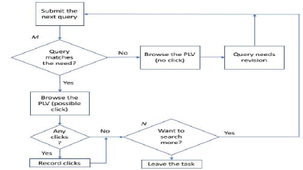
Figure 2. Task-centric Click Model with Macro Bernoulli variables $M$, $N$ labelled.

There are several important ways in which we have simplified the analysis and model as compared with the TCM of (Zhang et al., 2011). First, we do not consider the so-called ”duplicate bias” or the associated freshness variable of a SKU in our analysis, but we do indicate explicitly that the click variable depends on both relevance and other factors of SKU attractiveness. Second, we do not consider the last query in the query chain, or the clicks on the last PLV, as being in any way special. Third, (Zhang et al., 2011) perform inference and parameter tuning on the model, whereas in this work, at least, we use the model for a different purpose (see below). As a result (Zhang et al., 2011) need to adopt a particular click model inside the TCM (called the ”micro model”, or PLV/SERP interaction model) to fully specify the TCM. For our purposes the PLV interaction model could remain unspecified, but for the sake of concreteness, we specify a particular model, similar to the PBM, to govern the user’s interaction with the PLV, inside TCM in Figure 3, which is comparable to Figure 4 of (Zhang et al., 2011). Note that in comparison to their TCM model we have added the $A$ (attractiveness factor), eliminated the ”freshness” and ”previous examination factors”, and otherwise just made some changes of notation, namely using $S$ instead of $R$ to denote relevance/satisfaction in agreement with the notation of §4.1, and the more standard $r$ instead of $j$ for ”rank”. The important new variables present in the TCM are the following two relating to the session flow, rather than the internal search request flow (continuing the numbering (1)–(3) from §4.1):

1. The user’s intent being matched by query $i$, denoted by $M_{i}$;

2. The user submitting another search request after the $i$th query session, denoted by $N_{i}$.

A complete specification of our TCM consists of the template-based DAG representation of figure 3 together with the following parameterizations (compare (16)–(24) of (Zhang et al., 2011)):

$$P(M_{i}=1) =\alpha_{1}\in[0,1]$$

$$P(N_{i}=1|M_{i}=1) =\alpha_{2}\in[0,1]$$

$$P(E_{i,r}) =\gamma_{r}$$

$$P(A_{i,r}) =\alpha_{u,q}$$

$$P(S_{i,r}) =\sigma_{u,q}$$

$$M_{i}=0 \Rightarrow N_{i}=1$$

$$C_{i,r}=1 \Leftrightarrow M_{i}=1,\,E_{i,r}=1,\,S_{i,r}=1,\,A_{i,r}=1.$$

Resuming our discussion from §3, we are seeking a way to extract programmatically from the click logs a collection of triples $(q,d_{\rm rel},d_{\rm irrel})\in Q\times D\times D$ where ${\sigma_{d_{\rm rel},q}>\sigma_{d_{\rm irrel},q}}$, which is sufficiently ”adversarial”. The notion of ”adversarial” which we adopt, is that, first, $q$ belongs to a task (multi-query session) in the sense of the TCM, $q=q_{i^{\prime}}$ was preceded by a ”similar” query $q_{i}$, and $d_{\rm irrel}$, while irrelevant to $q_{i^{\prime}}$, is relevant to $q_{i}$. Note that this method of identifying the triples, at least heuristically, has a much higher chance of producing adversarial example because the similarity between $q_{i}$ and $q_{i^{\prime}}$ implies with high probability that ${\sigma_{d_{\rm rel},q_{i^{\prime}}}-\sigma_{d_{\rm irrel},q_{i^{\prime}}}}$ is much smaller than would be expected if we chose $d_{\rm irrel}$ from the SKU collection at random. Leaving aside the question, for the moment, of how to define search sessions (a point we will return to in Section 4), we can begin our approach to the construction of the triples by defining criteria which make it likely that the user’s true search intent is expressed by $q_{i^{\prime}}$, but not by $q_{i}$ (recall again that $i<i^{\prime}$, meaning $q_{i}$ is the earlier of the two queries):

1. The PLV for $q_{i}$ had no clicks: $C_{q_{i},u_{r}}=0,\;r=1,\ldots n$.

2. The PLV for $q_{i^{\prime}}$ had (at least) one click, on $r^{\prime}$: $C_{q_{i^{\prime}},u_{r^{\prime}}}=1$.

It turns out that relying on these criteria alone is too naïve. The problem is not the relevance $u_{q_{i^{\prime}},r^{\prime}}$ to $q_{i^{\prime}}$, but the supposed irrelevance of the $u_{q_{i},r}$ to $q_{i}$. In the terms of the TCM, this is because criterion (1), absence of any click on the PLV for $q_{i}$, does not in general imply that $M_{i}=0$. In (Zhang et al., 2011), the authors address this issue by performing parameter estimation using the click logs holistically. We make adopt a version this approach in future work. In the present work, we take a different approach, which is to examine the content of $q_{i}$, $q_{i^{\prime}}$ and add a filter (condition) that makes it much more likely that $M_{i}=0$, namely

1. The tokens of $q_{i^{\prime}}$ properly contain the tokens of $q_{i}$.

An example of a $(q_{i},q_{i^{\prime}})$ which satisfies (3) is (bookshelf, bookshelf with doors), whereas an example which does not satisfy (3) is (wooden bookshelf, bookshelf with doors): see the last line of Table 4. The idea behind (3) is in this situation, the user is refining her query to better match her true search intent, so we apply the term ”refinement” either to $q_{i^{\prime}}$ or to the pair $(q_{i},q_{i^{\prime}})$ as a whole. This addresses the issue that we need $M_{i}=0$ to conclude that $u_{i,r}$ are likely irrelevant to the query $q_{i^{\prime}}$.

However, there are still another couple of issues with using the triple $(q^{\prime},u_{q_{i^{\prime}},r^{\prime}},u_{q_{i},r})$ as a training example. The first stems from the observation that lack of click on $u_{q_{i},r}$ provides evidence for the irrelevance (to the user’s true intent $q^{\prime}$) only if it was examined, $E_{u_{q_{i},r}}=1$. This is the same observation as (7), but in the context of TCMs. We address this by adding a filter:

1. The rank $r$ of $u_{q_{i},r}\leq\rho$; $\rho$ a small integer parameter,

implying that $\gamma_{r}$ is relatively close to $1$. The second is an ”exceptional” type of situation where $M_{i}=0$, but certain $u_{i,r}$ on the PLV for $q_{i}$ are relevant to $q_{i^{\prime}}$. Consider as an example, the user issues the query $q_{i}$ ”rubber band”, then the query ”Acme rubber band” $q_{i^{\prime}}$, then clicks on an SKU $u_{q_{i^{\prime}},r^{\prime}}=u_{q_{i},r}$ she has previously examined on the PLV for $q_{i}$. This may indicate that the PLV for $q_{i}$ actually contained some results relevant to $q_{i^{\prime}}$, and examining such results reminded the user of her true search intent. In order to filter out the noise that from the dataset which would result from such cases, we add this condition:

1. $u_{q_{i^{\prime}},r^{\prime}}$ does not appear anywhere in the PLV for $q_{i}$.

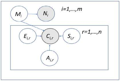
Figure 3. Template-based DAG representation of the TCM

5. Dataset Construction

Query	Relevant SKU	Irrelevant SKU
epson ink cartridges	Epson 252XL High-capacity Black Ink Cartridge	Canon CL-241XL Color Ink Cartridge
batteries aa	Sony S-am3b24a Stamina Plus Alkaline Batteries (aa; 24 Pk)	Durcell Quantum Alkaline Batteries — AAA, 12 Count
microsd 128gb	Sandisk Sdsqxvf-128g-an6ma Extreme Microsd Uhs-i Card With Adapter (128gb)	PNY 32GB MicroSDHC Card
accent chair	Acme Furniture Ollano Accent Chair — Fish Pattern — Dark Blue	ProLounger Wall Hugger Microfiber Recliner
bar stool red 2	Belleze©  Leather Hydraulic Lift Adjustable Counter Bar Stool Dining Chair Red — Pack of 2	Flash Furniture Modern Vinyl 23.25 In. — 32 In. Adjustable Swivel Barstool
bookshelf with doors	Better Homes and Gardens Crossmill Bookcase with Doors, Multiple Finishes	Way Basics Eco-Friendly 4 Cubby Bookcase

Table 4. Sample of Dataset , showing only original titles for SKU text

We group consecutive search requests by the same user into one session. Within each session, we extract semantically related query pairs $(q_{i},q_{i^{\prime}})$, $q_{i}$ submitted before $q_{i^{\prime}}$. The query $q_{i^{\prime}}$ is considered semantically related to the previously submitted $q_{i}$ if they satisfy condition (3) above in §4.3. We keep only $(q_{i},q_{i^{\prime}})$ satisfying (1)–(3) in §4.3. As explained in §4.3, if in addition the clicked SKU $u_{q_{i^{\prime}},r^{\prime}}$, and the unclicked SKUs $u_{q_{i},r}$ satisfy (4)–(5), we have high confidence that $M_{i}=0$ and $u_{q_{i},r}$ does not satisfy the user’s information need, whereas $M_{i^{\prime}}=1$ and $u_{q_{i^{\prime}},r^{\prime}}$ does. Therefore, based on our heuristic, we can construct an example for our dataset by constructing as many as $\rho$ training examples for each eligible click, of the form

$$(q,d_{\rm rel},d_{\rm irrel}):=(q_{i^{\prime}},\;u_{q_{i^{\prime}},r^{\prime}},\;u_{q_{i},r}),\;r=1,\ldots,\rho.$$

For our experiments, we processed logged search data on Jet.com from April to November 2017. We filtered to only search requests related to electronics and furniture categories, so as to enable fast experimentation. We implemented our construction method in Apache Spark (Zaharia et al., 2016). Our final dataset consists of around 3.6 million examples, with 130k unique $q$, 131k unique $d_{\rm rel}$, 275k unique $d_{\rm irrel}$, with 68k SKUs appearing as $d_{\rm rel}$ and $d_{\rm irrel}$ for different examples. Table 4 shows some examples extracted by our method.

In order to compensate for the relatively small number of unique $q$ in the dataset and the existence of concept drift in eCommerce, we formed the train-validate-split in the following manner rather than the usual practice in ML of using random splits: we reserved the first six months of data for training, the seventh month for validation, and the eighth (final) month for testing. Further, we filtered out from the validation set all examples with a $q$ seen in training; and from the test set, all examples with a $q$ seen in validation or training. This turned out to result in a (training:validation:test) ratio of $(75:2.5:1)$. Although the split is lopsided towards training examples, it still results in 46k test examples. We believe this drastic deletion of validation/test examples is well worth it to detect overfitting and distinguish true model learning from mere memorization.

We now give an overview of the principles used to form the SKU (document) text as actually encoded by the models. The query text is just whatever the user types into the search field. The SKU text is formed from the concatenating the SKU title with the text extracted from some other fields associated with the SKU in a database, some of which are free-text description, and others of which are more structured in nature. Finally, both the query and SKU texts are lowercased and normalized to clean up certain extraneous elements such as html tags and non-ASCII characters and to expand some abbreviations commonly found the SKU text. For example, an apostrophe immediately following numbers was turned into the token ”feet”. No models and no stemming or NLP analyzers, only regular expressions, are used in the text normalization.

6. Experimental Results

6.1. Details of Model Training

All of the supervised IR models were trained on one NVIDIA Tesla K80 GPU using PyTorch (Paszke et al., 2017), with the margin ranking loss:

$$L(f(q,d_{\rm rel}),f_{(}q,d_{\rm irrel}))=\max(0,f(q,d_{\rm irrel})-f(q,d_{\rm rel})+1).$$

We used the Adam optimizer (Kingma and Ba, 2014), with an initial learning rate of $1\times 10^{-4}$, using PyTorch’s built-in learning rate scheduler to decrease the learning rate in response to a plateau in validation loss. For the kernel-pooling model, it takes about $8$ epochs, with a run time of about $2.5$ hours assuming a batch-size of $512$, for the learning rate to reach $1\times 10^{-6}$, after which further decrease in the learning rate does not result in significant validation accuracy improvements. Also, for the kernel-pooling model, we explored the effect of truncating the SKU text at various lengths. In particular, we tried keeping the first $32$, $64$ and $128$ tokens of the text, and we report the results below. For the CLSM and Siamese models we tried changing the dimension of both $V$, the distributed query/document representations, and the number of channels of the $\mathrm{cnn}$ layer (dimension of input to $\mathrm{mlp}_{1}$) using values evenly spaced in logarithmic space between $32$ and $512$. We also tried $3$ different values of the dropout rate in these models.

For the Kernel-pooling model, we used word vectors from an unsupervised pre-training step, using the training/validation texts as the corpus. As our word2vec algorithm, we used the CBOW and Skipgram algorithms as implemented Gensim’s (Rehurek and Sojka, 2010) FastText wrapper. We observed no improvement in performance of the relevance model from changing the choice of word2vec algorithm or altering the word2vec hyperparameters from their default values. For the tf—idf baseline, we also used the Gensim library, without changing any of the default settings, to compile the idf (inverse document frequency) statistics.

6.2. Error Rate Comparison

Model	Validation	Test
Kernel-pooling, trainable embeddings
truncation length 32	68.63	65.62
truncation length 64	63.13	62.92
truncation length 128	70.16	73.97
Kernel-pooling, frozen embeddings
truncation length 64	66.13	65.40
tf—idf baseline	N/A	100.0

Table 5. Error rates of models, reported as percent of error rate of tf—idf baseline. Validation column reports error rate for the best (lowest) training epoch. Note that, in all experiments to date on our dataset, none of the distributed models (DSSM, CLSM, Siamese) have outperformed the baseline.

We have reported our main results, the error rates of the trained relevance models in Table 5. The most notable finding is that the kernel-pooling model, our main representative of the distributed class showed a sizable improvement over the baseline, and in our experiments thus far, none of the distributed representation models even matched the baseline. We found that the distributed models had adequate capacity to overfit the training data, but they are not generalizing well to the validation/test data. We will discuss ongoing efforts to correct this in §7 below. Another notable finding is that there is an ideal truncation length of the SKU texts for the kernel-pooling model, in our case around $2^{6}$ tokens, which allows the model enough information without introducing too much extraneous noise. Finally, following (Xiong et al., 2017), we also evaluated a variant of the kernel-pooling model where the word embeddings were ”frozen”, i.e. fixed at their initial word2vec values. Interestingly, unlike what was observed in (Xiong et al., 2017), we observed only a modest degredation in performance, as measured by overall error rate, from the model using the word2vec embeddings as compared with the full model. Based on the qualitative analysis of the learned embeddings, §6.3, we believe it is still worthwhile to train the full model.

Table 6. Training paths of Kernel Pooling Model With Different Hyperparameter Choices

6.3. Pre-trained versus fine-tuned embeddings

Similarly to (Xiong et al., 2017), we found that the main effect of the supervised retraining of the word embeddings was to decouple certain word pairs. Corresponding to Table 8 of their paper we have listed some examples of the moved word pairs in Table 7. The training decouples roughly twice as many word pairs as it moves closer together. In spite of the relatively modest gains to overall accuracy from the fine-tuning of embeddings, we believe this demonstrates the potential value of the fine-tuned embeddings for other search-related tasks.

From	To	Word Pairs
$\mu=0.8$	$\mu=0.1$	(male, female), (magenta, cyan)
$\mu=0.5$	$\mu=0.1$	(64gb, 128gb), (loveseat, pillows)
$\mu=0.1$	$\mu=-0.3$	(piece, sensations), (monitor, styling)
$\mu=0.5$	$\mu=-0.1$	(internal, external), (tv, hdtv)
$\mu=-0.1$	$\mu=0.3$	(vintage, component), (replacement, pedestal)

Table 7. Examples of moved word pairs

7. Conclusions

We showed how to construct a rich, adversarial dataset for eCommerce relevance. We demonstrated that one of the current state-of-art NIR models, namely the Kernel Pooling model, is able to reduce pairwise ranking errors on this dataset, as compared to the tf—idf baseline, by over a third. We observed that the distributional NIR models such as DSSM and CLSM overfit and do not learn to generalize well on this dataset. Because of the inherent advantages of distributional over local-interaction models, our first priority for ongoing work is to diagnose and overcome this overfitting so that the distributional models at least outperform the baseline. The work is proceeding along two parallel tracks. One is explore further architectures in the space of all possible NIR models to find ones which are easier to regularize. The other is to perform various forms of data augmentation, both in order to increase the sheer quantity of data available for the models to train on and to overcome any biases that the current data generation process may introduce.

- (1)
- Borisov et al. (2016) Alexey Borisov, Ilya Markov, Maarten de Rijke, and Pavel Serdyukov. 2016. A neural click model for web search. In Proceedings of the 25th International Conference on World Wide Web. International World Wide Web Conferences Steering Committee, 531–541.
- Chuklin et al. (2015) Aleksandr Chuklin, Ilya Markov, and Maarten de Rijke. 2015. Click models for web search. Synthesis Lectures on Information Concepts, Retrieval, and Services 7, 3 (2015), 1–115.
- Goldberg (2017) Yoav Goldberg. 2017. Neural Network Methods for Natural Language Processing. Synthesis Lectures on Human Language Technologies 37 (2017), 1–287.
- Gormley and Tong (2015) Clinton Gormley and Zachary Tong. 2015. Elasticsearch: The Definitive Guide: A Distributed Real-Time Search and Analytics Engine. O’Reilly Media, Inc.
- Huang et al. (2013) Po-Sen Huang, Xiaodong He, Jianfeng Gao, Li Deng, Alex Acero, and Larry Heck. 2013. Learning deep structured semantic models for web search using clickthrough data. In Proceedings of the 22nd ACM international conference on Conference on information & knowledge management. ACM, 2333–2338.
- Kingma and Ba (2014) Diederik P Kingma and Jimmy Ba. 2014. Adam: A method for stochastic optimization. arXiv preprint arXiv:1412.6980 (2014).
- Koller and Friedman (2009) Daphne Koller and Nir Friedman. 2009. Probabilistic graphical models: principles and techniques. MIT press.
- Kutiyanawala et al. (2018) Aliasgar Kutiyanawala, Prateek Verma, and Zheng Yan. 2018. Towards a simplified ontology for better e-commerce search. In Proceedings of the SIGIR 2018 Workshop on eCommerce (ECOM 18).
- Le and Mikolov (2014) Quoc Le and Tomas Mikolov. 2014. Distributed representations of sentences and documents. In Proceedings of the 31st International Conference on Machine Learning (ICML-14). 1188–1196.
- Li (2014) Hang Li. 2014. Learning to rank for information retrieval and natural language processing. Synthesis Lectures on Human Language Technologies 7, 3 (2014), 1–121.
- Mitra and Craswell (2017) Bhaskar Mitra and Nick Craswell. 2017. Neural Models for Information Retrieval. arXiv preprint arXiv:1705.01509 (2017).
- Mitra et al. (2017) Bhaskar Mitra, Fernando Diaz, and Nick Craswell. 2017. Learning to match using local and distributed representations of text for web search. In Proceedings of the 26th International Conference on World Wide Web. International World Wide Web Conferences Steering Committee, 1291–1299.
- Moore et al. (2018) John Moore, Joel Pfeiffer, Kai Wei, Rishabh Iyer, Denis Charles, Ran Gilad-Bachrach, Levi Boyles, and Eren Manavoglu. 2018. Modeling and Simultaneously Removing Bias via Adversarial Neural Networks. arXiv preprint arXiv:1804.06909 (2018).
- Mu et al. (2018) Cun Mu, Jun Zhao, Guang Yang, Jing Zhang, and Zheng Yan. 2018. Towards Practical Visual Search Engine Within Elasticsearch. In Proceedings of the SIGIR 2018 Workshop on eCommerce (ECOM 18).
- Paszke et al. (2017) Adam Paszke, Sam Gross, Soumith Chintala, Gregory Chanan, Edward Yang, Zachary DeVito, Zeming Lin, Alban Desmaison, Luca Antiga, and Adam Lerer. 2017. Automatic differentiation in PyTorch. In NIPS-W.
- Pennington et al. (2014) Jeffrey Pennington, Richard Socher, and Christopher Manning. 2014. Glove: Global vectors for word representation. In Proceedings of the 2014 conference on empirical methods in natural language processing (EMNLP). 1532–1543.
- Rehurek and Sojka (2010) Radim Rehurek and Petr Sojka. 2010. Software Framework for Topic Modelling with Large Corpora. In Proceedings of the LREC 2010 Workshop on New Challenges for NLP Frameworks. ELRA, Valletta, Malta, 45–50.
- Robertson et al. (2009) Stephen Robertson, Hugo Zaragoza, et al. 2009. The probabilistic relevance framework: BM25 and beyond. Foundations and Trends® in Information Retrieval 3, 4 (2009), 333–389.
- Rygl et al. (2017) Jan Rygl, Jan Pomikalek, Radim Rehurek, Michal Ruzicka, Vit Novotny, and Petr Sojka. 2017. Semantic Vector Encoding and Similarity Search Using Fulltext Search Engines. In Proceedings of the 2nd Workshop on Representation Learning for NLP. 81–90.
- Shen et al. (2014) Yelong Shen, Xiaodong He, Jianfeng Gao, Li Deng, and Grégoire Mesnil. 2014. A latent semantic model with convolutional-pooling structure for information retrieval. In Proceedings of the 23rd ACM International Conference on Conference on Information and Knowledge Management. ACM, 101–110.
- Smiley et al. (2015) David Smiley, Eric Pugh, Kranti Parisa, and Matt Mitchell. 2015. Apache Solr enterprise search server. Packt Publishing Ltd.
- Trends (2018) Google Trends. 2018. Year in Search 2017. Retrieved April 29, 2018 from https://trends.google.com/trends/yis/2017/GLOBAL/
- Tu et al. (2017) Zhucheng Tu, Matt Crane, Royal Sequiera, Junchen Zhang, and Jimmy Lin. 2017. An Exploration of Approaches to Integrating Neural Reranking Models in Multi-Stage Ranking Architectures. arXiv preprint arXiv:1707.08275 (2017).
- Venturebeat.com (2013) Venturebeat.com. 2013. How Google Searches 30 Trillion Web Pages 100 Billion Times a month. Retrieved April 29, 2018 from https://venturebeat.com/2013/03/01/how-google-searches-30-trillion-web-pages-100-billion-times-a-month/
- Wikipedia (2018) Wikipedia. 2018. Tf—idf. Retrieved April 30, 2018 from https://en.wikipedia.org/wiki/Tf%E2%80%93idf
- Xiong et al. (2017) Chenyan Xiong, Zhuyun Dai, Jamie Callan, Zhiyuan Liu, and Russell Power. 2017. End-to-end neural ad-hoc ranking with kernel pooling. In Proceedings of the 40th International ACM SIGIR Conference on Research and Development in Information Retrieval. ACM, 55–64.
- Zaharia et al. (2016) Matei Zaharia, Reynold S Xin, Patrick Wendell, Tathagata Das, Michael Armbrust, Ankur Dave, Xiangrui Meng, Josh Rosen, Shivaram Venkataraman, Michael J Franklin, et al. 2016. Apache spark: a unified engine for big data processing. Commun. ACM 59, 11 (2016), 56–65.
- Zhang et al. (2011) Yuchen Zhang, Weizhu Chen, Dong Wang, and Qiang Yang. 2011. User-click modeling for understanding and predicting search-behavior. In Proceedings of the 17th ACM SIGKDD international conference on Knowledge discovery and data mining. ACM, 1388–1396.