THE STOCHASTIC FITZHUGH-NAGUMO NEURON MODEL IN THE EXCITABLE REGIME EMBEDS A LEAKY INTEGRATE-AND-FIRE MODEL

Abstract

In this paper, we provide a complete mathematical construction for a stochastic leaky-integrate-and-fire model (LIF) mimicking the interspike interval (ISI) statistics of a stochastic FitzHugh-Nagumo neuron model (FHN) in the excitable regime, where the unique fixed point is stable. Under specific types of noises, we prove that there exists a global random attractor for the stochastic FHN system. The linearization method is then applied to estimate the firing time and to derive the associated radial equation representing a LIF equation. This result confirms the previous prediction in [Ditlevsen and Greenwood, 2013] for the Morris-Lecar neuron model in the bistability regime consisting of a stable fixed point and a stable limit cycle.

60GXX, 92BXX

1 Introduction

Mathematical modeling has emerged as an important tool to handle the overwhelming structural complexity of neuronal processes and to gain a better understanding of their functioning from the dynamics of their model equations. However, the mathematical analysis of biophysically realistic neuron models such as the 4-dimensional Hodgkin-Huxley (HH) [Hodgkin and Huxley, 1952] and the 2-dimensional Morris-Lecar (ML) [Morris and Lecar, 1981] equations is difficult, as a result of a large parameter space, strong nonlinearities, and a high dimensional phase space of the model equations. The search for simpler, mathematically tractable (small parameter space, weaker nonlinearities, low dimensional phase space) neuron models that still capture all, or at least some important dynamical behaviors of biophysical neurons (HH and ML) has been an active area of research.

The efforts in this area of research have resulted in easily computable neuron models which mimic some of the dynamics of biophysical neuron models. One of the resulting models is the 2-dimensional FitzHugh-Nagumo (FHN) neuron model [FitzHugh, 1961]. The FHN model has been so successful, because it is at the same time mathematically simple and produces a rich dynamical behavior that makes it a model system in many regards, as it reproduces the main dynamical features of the HH model. In fact, the HH model has two types of variables, and each type then is combined into a single variable in FHN: The ($V,m$) variables of HH correspond to the $v$ variable in FHN, whose fast dynamics represents excitability; the ($h,n$) variables correspond to the $w$ variable, whose slow dynamics represents accommodation and refractoriness.

The fact that the FHN model is low dimensional makes it possible to visualize the solution and to explain in geometric terms important phenomena related to the excitability and action potential generation mechanisms observed in biological neurons. Of course, this comes at the expense of numerical agreement with the biophysical neuron models [Yamakou, 2018]. The purpose of the model is not a close match with biophysically realistic high dimensional models, but rather a mathematical explanation of the essential dynamical mechanism behind the firing of a neuron. Moreover, the analysis of such simpler neuron models may lead to the discovery of new phenomena, for which we may then search in the biological neuron models and also in experimental preparations.

There is, however, an even simpler model than FHN, the leaky integrate-and-fire model (LIF). This is the simplest reasonable neuron model. It only requires a few basic facts about nerve cells: they have membranes, they are semipermeable, and they are polarizable. This suffices to deduce a circuit equivalent to that of the membrane potential of the neuron: a resistor-capacitor circuit. Such circuits charge up slowly when presented with a current, cross a threshold voltage (a spike), then slowly discharge. This behavior is modeled by a simple 1D equation together with a reset mechanism: the leaky integrate-and-fire neuron model equation [Gerstner and Kistler, 2002]. Combining sub-threshold dynamics with firing rules has led to a variety of 1D leaky integrate-and-fire descriptions of a neuron with a fixed membrane potential firing threshold [Gerstner and Kistler, 2002, Lansky and Ditlevsen, 2008], or with a firing rate depending more sensitively on the membrane potential [Pfister et al., 2006]. In contrast to $n-$dimensional neuron models, $n\geq 2$, such as the HH, ML, and FHN models, the LIF class of neuron models is less expensive in numerical simulations, which is an essential advantage when a large network of coupled neurons is considered.

Noise is ubiquitous in neural systems and it may arise from many different sources. One source may come from synaptic noise, that is, the quasi-random release of neurotransmitters by synapses or random synaptic input from other neurons. As a consequence of synaptic coupling, real neurons operate in the presence of synaptic noise. Therefore, most works in computational neuroscience address modifications in neural activity arising from synaptic noise. Its significance can however be judged only if its consequences can be separated from the internal noise, generated by the operations of ionic channels [Calvin and Stevens, 1967]. The latter is channel noise, that is, the random switching of ion channels. In many papers channel noise is assumed to be minimal, because typically a large number of ion channels is involved and fluctuations should average out, and therefore, the effects of synaptic noise should dominate. Consequently, channel noise is frequently ignored in the mathematical modeling. However, the presence of channel noise can also greatly modify the behavior of neurons [White et al., 2000]. Therefore, in this paper, we study the effect of channel noise. Specifically, we add a noise term to the right-hand side of the gating equations (the equation for the ionic current variable).

In the stochastic model, the deterministic fixed point is no longer a solution of the system. The fixed point necessarily needs to vary and adapt to the noise. To account for this, in the theory of random dynamical systems, the notion of a random dynamical attractor was developed as a substitute for deterministic attractors in the presence of noise. In the first part of this paper, we therefore prove that our system admits a global random attractor, for both additive and multiplicative channel noises. This can be seen as a theoretical grounding of our setting.

In [Ditlevsen and Greenwood, 2013], it was shown that a stochastic LIF model constructed with a radial Ornstein-Uhlenbeck process is embedded in the ML model (in a bistable regime consisting of a fixed point and limit cycle) as an integral part of it, closely approximating the sub-threshold fluctuations of the ML dynamics. This result suggests that the firing pattern of a stochastic ML can be recreated using the embedded LIF together with a ML stochastic firing mechanism. The LIF model embedded in the ML model captures sub-threshold dynamics of a combination of the membrane potential and ion channels. Therefore, results that can be readily obtained for LIF models can also yield insight about ML models. In the second part of this paper, we here address the problem to obtain a stochastic LIF model mimicking the interspike interval (ISI) statistics of the stochastic FHN model in the excitable regime, where the unique fixed point is stable. Theoretically, we obtain such a LIF model by reducing the 2D FHN model to the one dimensional system that models the distance of the solution to the random attractor as shown in the first part of the paper. In fact, we show that this distance can be approximated to the fixed point, up to a rescaling, as the Euclidean norm $R_{t}$ of the solution of the linearization of the stochastic FHN equation along the deterministic equilibrium point, and hence the LIF model is approximated by the equation for $R_{t}$. An action potential (a spike) is produced when $R_{t}$ exceeds a certain firing threshold $R_{t}\geq r_{0}>0$. After firing the process is reset and time is back to zero. The ISI $\tau_{0}$ is identified with the first-passage time of the threshold, $\tau_{0}=\inf\{t>0:R_{t}\geq r_{0}>0\}$, which then acts as an upper bound of the spiking time $\tau$ of the original system. By defining the firing as a series of first-passage times, the 1D radial process $R_{t}$ together with a simple firing mechanism based on the detailed FHN model (in the excitable regime), the firing statistics is shown to reproduce the 2D FHN ISI distribution. We also show that $\tau$ and $\tau_{0}$ share the same distribution.

The rest of the paper is organized as follows: Sect. 2 introduces the deterministic version of the FHN neuron model, where we determine the parameter values for which the model is in the excitable regime. In Sect. 3, we prove the existence of a global random attractor of the random dynamical system generated by the stochastic FHN equation; and furthermore derive a rough estimate for the firing time using the linearization method. The corresponding stochastic LIF equation is then derived in Sect. 4 and its distribution of interspike-intervals is found to numerically match the stochastic FHN model.

2 The deterministic model and the excitable regime

In the fast time scale $t$, the deterministic FHN neuron model is

(2.1) $$\begin{cases}dv_{t}&=(v_{t}-\displaystyle{\frac{v_{t}^{3}}{3}}-w_{t}+I)dt=f(v_{t},w_{t})dt,\\ dw_{t}&=\varepsilon(v_{t}+\alpha-\beta w_{t})dt=g(v_{t},w_{t})dt.\end{cases}$$

where $v_{t}$ is the activity of the membrane potential and $w_{t}$ is the recovery current that restores the resting state of the model. $I$ is a constant bias current which can be considered as the effective external input current. $0<\varepsilon:=t/\tau\ll 1$ is a small singular perturbation parameter which determines the time scale separation between the fast $t$ and the slow time scale $\tau$. Thus, the dynamics of $v_{t}$ is much faster than that of $w_{t}$. $\alpha$ and $\beta$ are parameters.

The deterministic critical manifold $\mathcal{C}_{0}$ defining the set of equilibria of the layer problem associated to Eq. (2.1) (i.e., the equation obtained from Eq. (2.1) in the singular limit $\epsilon=0$, see [Kuehn, 2015] for a comprehensive introduction to slow-fast analysis), is obtained by solving $f(v,w)=0$ for $w$. Thus, it is given by

(2.2) $$\mathcal{C}_{0}=\left\{(v,w)\in\mathbb{R}^{2}:w=\displaystyle{v-\frac{v^{3}}{3}+I}\right\}.$$

We note that for Eq. (2.1), $\mathcal{C}_{0}$ coincides with the $v$-nullcline (the red curve in Fig. (1)). The stability of points on $\mathcal{C}_{0}$ as steady states of the layer problem associated to Eq. (2.1) is determined by the Jacobian scalar $(D_{v}f)(v,w)=1-v^{2}$. This shows that on the critical manifold, points with $|v|>1$ are stable while points with $|v|<1$ are unstable. It follows that the branch $v_{-}^{*}(w)\in(-\infty,-1)$ is stable, $v_{0}^{*}(w)\in(-1,1)$ is unstable, and $v_{+}^{*}(w)\in(1,+\infty)$ is stable.

The set of fixed points $(v_{e},w_{e})$ which define the resting states of the neuron is given by

(2.3) $$\{(v,w)\in\mathbb{R}^{2}:f(v,w)=g(v,w)=0\}.$$

The sign of the discriminant $\bigtriangleup=(1/\beta-1)^{3}+\frac{9}{4}(\alpha/\beta-I)^{2}$, determines the number of fixed points. $\mathcal{C}_{0}$ can therefore intersect the $w$-nullcline ($w=\frac{v+\alpha}{\beta}$) at one, two or three different fixed points. We assume in this paper that $\bigtriangleup>0$, in which case we have a unique fixed point given by

(2.4) $$\begin{cases}\displaystyle{v_{e}=\sqrt[3]{-\frac{q}{2}-\sqrt{\Delta}}+\sqrt[3]{-\frac{q}{2}+\sqrt{\Delta}}}\\ w_{e}=\frac{1}{\beta}(v_{e}+\alpha).\end{cases}$$

where

$$p=3\Big{(}\frac{1}{\beta}-1\Big{)},\qquad q=3\Big{(}\frac{\alpha}{\beta}-I\Big{)}.$$

Here, we want to consider the neuron in the excitable regime [Ditlevsen and Greenwood, 2013]. A neuron is in the excitable regime when starting in the basin of attraction of a unique stable fixed point, an external pulse will result into at most one large excursion (spike) into the phase space after which the phase trajectory returns back to this fixed point and stays there [Izhikevich, 2007].

In order to have Eq. (2.1) in the excitable regime, we choose $I,\alpha,$ and $\beta$ such that $\Delta>0$ (i.e., a unique fixed point) and $\varepsilon$ such that the Jacobian (the linearization matrix $M$) of Eq.(2.1) at the fixed point $(v_{e},w_{e})$ has a pair of complex conjugate eigenvalues

$$-\mu\pm i\nu=\frac{1}{2}(1-v_{e}^{2}-\epsilon\beta)\pm\frac{i}{2}\sqrt{4\epsilon-(1-v_{e}^{2}+\epsilon\beta)^{2}}$$

with negative real part (i.e., a stable fixed point). In that case, $(v_{e},w_{e})$ is the only stationary state and there is no limit cycle of system (2.1). In other words, $(v_{e},w_{e})$ is the global attractor of the system [Izhikevich, 2007]. Moreover, to apply the averaging technique [Baxendale and Greenwood, 2011], it is necessary that $\mu\ll\nu$, we therefore use through this paper the following parameters of system: $I=0.265,\alpha=0.7,\beta=0.75,\varepsilon=0.08$ so that $(v_{e},w_{e})=(-1.00125,-0.401665)$ is the unique stable fixed point and $\frac{\mu}{\nu}=0.111059\ll 1$. Fig. (1) shows the neuron in the excitable regime. Notice that although every trajectory finally converges to the fixed point, only a small change in the location of the starting point will result in different behavior of the trajectories (see the blue and purple curves).

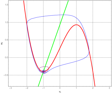
Figure 1: The critical manifold $\mathcal{C}_{0}$ (red curve) and the $w$-nullcline (green line) intersect at the unique and stable fixed point $(v_{e},w_{e})=(-1.00125,-0.401665)$. Two deterministic trajectories are shown, the purple curve starts at $(-1.00125,-0.45)$ and the blue curve starts at $(-1.00125,-0.46)$. Parameters of system $I=0.265,\alpha=0.7,\beta=0.75,\varepsilon=0.08$ and the real time for trajectories $T=1000.$

3 The stochastic model

We consider this stochastic FHN model

(3.1) $$\begin{cases}dv_{t}&=f(v_{t},w_{t})dt,\\ dw_{t}&=g(v_{t},w_{t})dt+h(w_{t})\circ dB_{t},\end{cases}$$

where the deterministic fields $f$ and $g$ are given in Eq. (2.1). There are two important cases: either $h(w)=\sigma_{0}$ (additive channel noise) or $h(w)=\sigma_{0}w$ (multiplicative channel noise). $\circ dB_{t}$ stands for the Stratonovich stochastic integral with respect to the Brownian motion $B_{t}$.

Fig. 2 shows the phase portraits of Eq. (3.1) starting with the initial condition $(v_{0},w_{0})=(-1.00125,-0.4)$, which is in the vicinity of the stable fixed point. Given an initial condition close to the stable fixed point $(v_{e},w_{e})=(-1.00125,-0.401665)$, the trajectory of the stochastic system might first rotate around the stable fixed point but then the noise may trigger a spike, that is, a large excursion into the phase space, before returning to the neighbourhood of the fixed point; the process repeats itself leading to alternations of small and large oscillations. A similar behavior can be observed when the deterministic system with an additional limit cycle is perturbed by noise (as seen in the bistable system [Ditlevsen and Greenwood, 2013]).

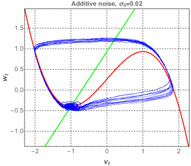
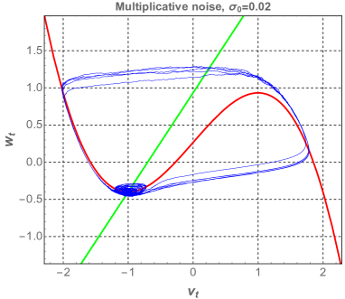
Figure 2: Random trajectory of Eq. (3.1) in the excitable regime with chosen parameters of system and the initial condition $(v_{0},w_{0})=(-1.00125,-0.4)$ for both additive and multiplicative noise (we use the StochasticRungeKutta method in Mathematica with the real time $T=1000$ and the step size $h=0.01$).

Fig. 3 shows that the spiking frequency increases as the amplitude of the noise increases. For a fixed simulation time $T=1000$, the system spikes only rarely, if at all, when the amplitude $\sigma_{0}\leq 0.005$, but spikes more frequently when $\sigma_{0}$ increases. This is similar for multiplicative noise.

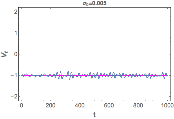
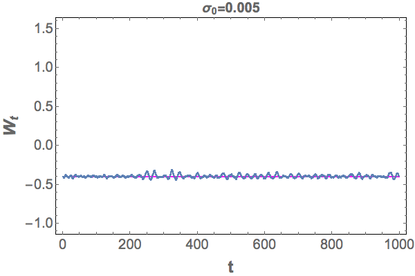
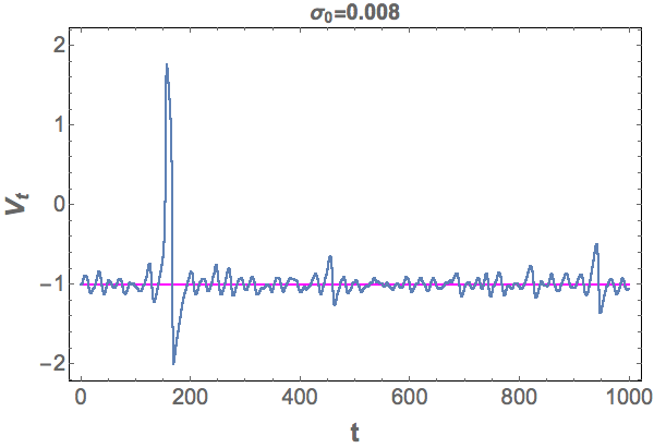
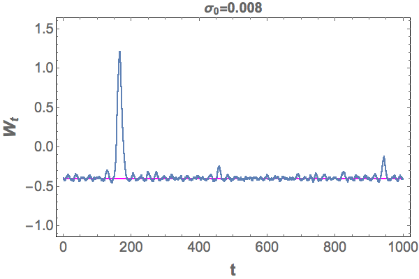
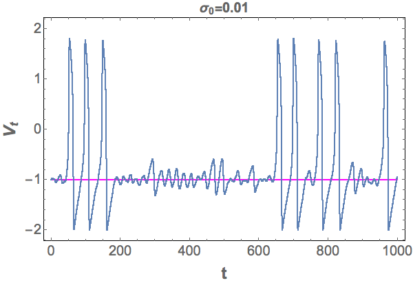
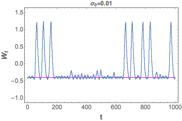
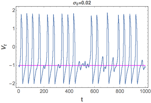
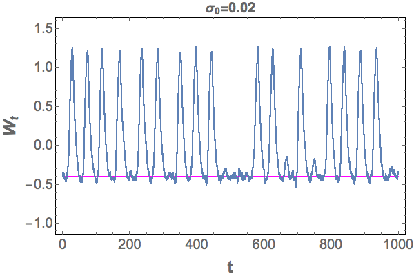
Figure 3: The components (left column: $V_{t}$, right column: $W_{t}$) of a random trajectory of Eq. (3.1) in the excitable regime with chosen parameters of system and the initial condition $(v_{0},w_{0})=(-1.00125,-0.4)$ for additive noise with $\sigma_{0}\in\{0.005,0.008,0.01,0.02\},T=1000,h=0.01$.

Let $\mathbf{X}=(v,w)^{T}$ and $F(\mathbf{X}),H(\mathbf{X})\in\mathbb{R}^{2}$ be the drift and diffusion coefficients of (3.1). The stochastic system is then of the form

(3.2) $$d\mathbf{X}_{t}=F(\mathbf{X}_{t})dt+H(\mathbf{X}_{t})\circ dB_{t},$$

where $H(\mathbf{X})=(0,\sigma_{0})^{\rm T}$ for additive noise and $H(\mathbf{X})=\begin{pmatrix}0&0\\ 0&\sigma_{0}\end{pmatrix}\mathbf{X}=B\mathbf{X}$ for multiplicative noise. It is easy to check that $F$ is dissipative in the weak sense, i.e.

$$\langle\mathbf{X}_{1}-\mathbf{X}_{2},F(\mathbf{X}_{1})-F(\mathbf{X}_{2})\rangle = (v_{1}-v_{2})^{2}\Big{[}1-\frac{1}{3}(v_{1}^{2}+v_{1}v_{2}+v_{2}^{2})\Big{]}$$

$$-(1-\epsilon)(v_{1}-v_{2})(w_{1}-w_{2})-\epsilon\beta(w_{1}-w_{2})^{2}$$

$$\leq (v_{1}-v_{2})^{2}\Big{[}1-\frac{1}{12}(v_{1}-v_{2})^{2}\Big{]}$$

$$+\frac{(1-\epsilon)^{2}}{2\epsilon\beta}|v_{1}-v_{2}|^{2}+\frac{\epsilon\beta}{2}|w_{1}-w_{2}|^{2}-\epsilon\beta(w_{1}-w_{2})^{2}$$

$$\leq -\frac{1}{12}\Bigg{(}|v_{1}-v_{2}|^{2}-6\Big{(}1+\frac{\epsilon\beta}{2}+\frac{(1-\epsilon)^{2}}{2\epsilon\beta}\Big{)}\Bigg{)}^{2}$$

$$+3\Big{(}1+\frac{\epsilon\beta}{2}+\frac{(1-\epsilon)^{2}}{2\epsilon\beta}\Big{)}^{2}-\frac{\epsilon\beta}{2}(|v_{1}-v_{2}|^{2}+|w_{1}-w_{2}|^{2})$$

(3.4) $$\leq a-b\|\mathbf{X}_{1}-\mathbf{X}_{2}\|^{2}$$

where

$$a:=3\Big{(}1+\frac{\epsilon\beta}{2}+\frac{(1-\epsilon)^{2}}{2\epsilon\beta}\Big{)}^{2},\qquad b:=\frac{\epsilon\beta}{2}.$$

On the other hand, we have

(3.5) $$|H(\mathbf{X}_{1})-H(\mathbf{X}_{2})|\leq\sigma_{0}\Big{|}w_{1}-w_{2}\Big{|}\leq\sigma_{0}\|\mathbf{X}_{1}-\mathbf{X}_{2}\|,$$

for multiplicative noise, while $|H(\mathbf{X}_{1})-H(\mathbf{X}_{2})|\equiv 0$ for additive noise, so $H$ is globally Lipschitz continuous.

3.1 The existence of a random attractor

In the sequel, we are going to prove that there exists a unique solution $\mathbf{X}(\cdot,\omega,\mathbf{X}_{0})$ of (3.1) and the solution then generates a so-called random dynamical system (see e.g. [Arnold, 1998, Chapters 1-2]).
More precisely, let $(\Omega,\mathcal{F},\mathbb{P})$ be a probability space on which our Brownian motion $B_{t}$ is defined. In our setting, $\Omega$ can be chosen as $C^{0}(\mathbb{R},\mathbb{R})$, the space of continuous real functions on $\mathbb{R}$ which are zero at zero, equipped with the compact open topology given by the uniform convergence on compact intervals in $\mathbb{R}$, $\mathcal{F}$ as $\mathcal{B}(C^{0})$, the associated Borel-$\sigma$-algebra and $\mathbb{P}$ as the Wiener measure. The Brownian motion $B_{t}$ can then be constructed as the canonical version $B_{t}(\omega):=\omega(t)$.
On this probability space we construct a dynamical system $\theta$ as the Wiener shift

(3.6) $$\theta_{t}m(\cdot)=m(t+\cdot)-m(t),\quad\forall t\in\mathbb{R},\forall m\in\bar{\Omega}.$$

Then $\theta_{t}(\cdot):\Omega\to\Omega$ satisfies the group property, i.e. $\theta_{t+s}=\theta_{t}\circ\theta_{s}$ for all $t,s\in\mathbb{R}$, and is $\mathbb{P}$-preserving, i.e. $\mathbb{P}(\theta_{t}^{-1}(A))=\mathbb{P}(A)$ for every $A\in\mathcal{F}$, $t\in\mathbb{R}$. The quadruple $((\Omega,\mathcal{F},\mathbb{P},(\theta_{t})_{t\in\mathbb{R}})$ is called a metric dynamical system.
Given such a probabilistic setting, Theorem 3.1 below proves that the solution mapping $\varphi:\mathbb{R}\times\Omega\times\mathbb{R}^{2}\to\mathbb{R}^{2}$ defined by $\varphi(t,\omega)\mathbf{X}_{0}:=\mathbf{X}(t,\omega,\mathbf{X}_{0})$ is a random dynamical system satisfying $\varphi(0,\omega)\mathbf{X}_{0}=\mathbf{X}_{0}$ and the cocycle property

(3.7) $$\varphi(t+s,\omega)\mathbf{X}_{0}=\varphi(t,\theta_{s}\omega)\circ\varphi(s,\omega)\mathbf{X}_{0},\qquad\forall t,s\in\mathbb{R},\omega\in\Omega,\mathbf{X}_{0}\in\mathbb{R}^{2}$$

To investigate the asymptotic behavior of the system under the influence of noise, we shall first check the effect of the noise amplitude on firing. Under the stochastic scenario, the fixed point $\mathbf{X}_{e}=(v_{e},w_{e})$ is no longer the stationary state of the stochastic system (3.1). Instead, we need to find the global asymptotic state as a compact random set $A(\omega)\in\mathbb{R}^{2}$ depending measurably on $\omega\in\Omega$ such that $A$ is invariant under $\varphi$, i.e. $\varphi(t,\omega)A(\omega)=A(\theta_{t}\omega)$, and attracts all other compact random sets $D(\omega)$ in the pullback sense, i.e.

$$\lim\limits_{t\to\infty}d(\varphi(t,\theta_{-t}\omega)D(\theta_{-t}\omega)|A(\omega))=0,$$

where $d(B|A)$ is the Hausdorff semi-distance. Such a structure is called a random attractor (see e.g. [Crauel et al., 1997] or [Arnold, 1998, Chapter 9]).
The following theorem ensures that the stochastic system (3.1) has a global random pullback attractor. The proof is provided in the Appendix.

Theorem 3.1.

There exists a unique solution of (3.2) which generates a random dynamical system. Moreover, the system possesses a global random pullback attractor.

Theorem 3.1 shows that every trajectory would in the long run converge to the global random attractor. The structure and the inside dynamics of the global random attractor are still open issues which might help understand the firing mechanism.

3.2 The normal form at the equilibrium point

One way to study the dynamics of the stochastic system (3.1) is through its linearization. Therefore, in this section, we shall study the dynamics of (3.1) in a small vicinity of the fixed point $\mathbf{X}_{e}=(v_{e},w_{e})$. To do that, consider the shift system w.r.t. the fixed point $\mathbf{X}_{e}$ which has the form

(3.8) $$d(\mathbf{X}_{t}-\mathbf{X}_{e}) = [F(\mathbf{X}_{t})-F(\mathbf{X}_{e})]dt+H(\mathbf{X}_{t})\circ dB_{t}$$

$$= \Big{[}DF(\mathbf{X}_{e})(\mathbf{X}_{t}-\mathbf{X}_{e})+\bar{F}(\mathbf{X}_{t}-\mathbf{X}_{e})\Big{]}dt+H(\mathbf{X}_{t})\circ dB_{t},$$

with initial point $\mathbf{X}_{0}-\mathbf{X}_{e}$, where $DF(\mathbf{X}_{e})$ is the linearized matrix of $F$ at $\mathbf{X}_{e}$, $\bar{F}$ is the nonlinear term such that

$$\|\bar{F}(\mathbf{X}-\mathbf{X}_{e})\| =\Bigg{\|}\begin{pmatrix}\frac{1}{3}|v+2v_{e}|(v-v_{e})^{2}\\ 0\end{pmatrix}\Bigg{\|}$$

$$\leq\gamma(r)\|\mathbf{X}-\mathbf{X}_{e}\|,\qquad\forall\|\mathbf{X}-\mathbf{X}_{e}\|\leq r$$

for an increasing function $\gamma(\cdot):\mathbb{R}_{+}\to\mathbb{R}_{+}$, $r\mapsto\frac{r^{2}}{3}+|v_{e}|r$, which implies that $\lim\limits_{r\to 0}\gamma(r)=0$. Since $H(\mathbf{X})$ is either a constant or a linear function, we prove below that system (3.8) can be well approximated by its linearized system

(3.9) $$d{\bar{\mathbf{X}}}_{t}=DF(\mathbf{X}_{e})\bar{\mathbf{X}}_{t}dt+H(\bar{\mathbf{X}}_{t}+\mathbf{X}_{e})\circ dB_{t},\qquad\bar{\mathbf{X}}_{0}=\mathbf{X}_{0}-\mathbf{X}_{e}.$$

Theorem 3.2.

Given $\|\mathbf{X}_{0}-\mathbf{X}_{e}\|<r$ and equations (3.8), (3.9), define the stopping time $\tau=\inf\{t>0:\|\mathbf{X}_{t}-\mathbf{X}_{e}\|\geq r\}$. Then there exists a constant $C$ independent of $r$ such that for any $t\geq 0$, the following estimates hold

• For additive noise

  (3.10) $$\sup_{t\leq\tau}\|\mathbf{X}_{t}-\mathbf{X}_{e}-\bar{\mathbf{X}}_{t}\|\leq C\gamma(r)r.$$

• For multiplicative noise

  (3.11) $$E\|\mathbf{X}_{t\wedge\tau}-\mathbf{X}_{e}-\bar{\mathbf{X}}_{t\wedge\tau}\|^{2}\leq C\gamma^{2}(r)r^{2}.$$

The proof is provided in the Appendix. In practice we can even approximate (3.8) by the following linear system with additive noise

(3.12) $$d{\tilde{\mathbf{X}}}_{t}=DF(\mathbf{X}_{e})\tilde{\mathbf{X}}_{t}dt+H(\mathbf{X}_{e})\circ dB_{t},\qquad\tilde{\mathbf{X}}_{0}=\mathbf{X}_{0}-\mathbf{X}_{e}.$$

By the same arguments as in the proof of Theorem 3.2, we can prove the following estimate

(3.13) $$E\|\mathbf{X}_{t\wedge\tau}-\mathbf{X}_{e}-\tilde{\mathbf{X}}_{t\wedge\tau}\|^{2}\leq Cr_{0}^{2},$$

for the same stopping time $\tau=\inf\{t>0:\|\mathbf{X}_{t}-\mathbf{X}_{e}\|\geq r_{0}\}$.

Another comparison between the processes $\{\mathbf{X}_{t}-\mathbf{X}_{e}\}_{t}$ and $\{\bar{\mathbf{X}}_{t}\}_{t}$ can be obtained by using power spectral density estimation (see, for example, [Fan and Yao, 2003, Chapter 7]). In Fig. 4, the estimated spectral densities of the shifted original and the linearized process are plotted. The spectral densities are estimated from paths started from $0$ to $50$ ms of subthreshold fluctuations, and scaled to have the same maximum at $40$.

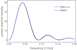
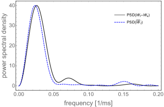
Figure 4: The process $\{\mathbf{X}_{t}-\mathbf{X}_{e}\}_{t}$ (3.8) and the process $\{\bar{\mathbf{X}}_{t}\}_{t}$ (3.9) with the chosen parameters of system, $\sigma_{0}=0.01$ and the same starting point $(v_{0}-v_{e},w_{0}-w_{e})$ are compared by using the power spectral density. Their spectrum densities are well approximated.

4 The embedded LIF model

In this section, we present two constructive methods to obtain $1$-D LIF models corresponding to the stochastic FHN in the excitable regime in Eq. (3.1). The first method follows [Baxendale and Greenwood, 2011] (see also [Ditlevsen and Greenwood, 2013]) by constructing the so-called radial Ornstein-Uhlenbeck equation. More precisely, we rewrite the linearized system (3.9) in the form

(4.1) $$d\bar{\mathbf{X}}_{t}=M\bar{\mathbf{X}}_{t}dt+\begin{pmatrix}0&0\\ 0&\sigma_{0}\end{pmatrix}d\mathbf{B}_{t},$$

where $M=DF(\mathbf{X}_{e})$ and $\mathbf{B}_{t}=\begin{pmatrix}B^{\prime}_{t}\\ B_{t}\end{pmatrix}$ is a $2$-D standard Brownian motion. For chosen parameters, $M$ has a pair of complex conjugate eigenvalues $-\mu\pm i\nu$ with $\mu=0.0312496,\nu=0.281378$. By transformation $\bar{\mathbf{Y}}_{t}=Q^{-1}\bar{\mathbf{X}}_{t}$ with $Q=\begin{pmatrix}-\nu&m_{11}+\mu\\ 0&m_{21}\end{pmatrix}$ we obtain

(4.2) $$d\bar{\mathbf{Y}}_{t}=A\bar{\mathbf{Y}}_{t}dt+Cd\mathbf{B}_{t},$$

where

$$A=\begin{pmatrix}-\mu&\nu\\ -\nu&-\mu\end{pmatrix}=\begin{pmatrix}-0.0312496&0.281378\\ -0.281378&-0.0312496\end{pmatrix};$$

$$C=Q^{-1}\begin{pmatrix}0&0\\ 0&\sigma_{0}\end{pmatrix}.$$

We note that $\frac{\mu}{\nu}=0.111059\ll 1$, therefore, by applying the technique of time average from [Baxendale and Greenwood, 2011, Theorem 1], $\bar{\mathbf{Y}}_{t}$ can be approximated by an Ornstein-Uhlenbeck process up to a rotation, i.e.

$$\bar{\mathbf{Y}}_{t}\sim\bar{\mathbf{Y}}^{app}_{t}:=\frac{\sigma}{\sqrt{\mu}}Rot_{-\nu t}\bar{\mathbf{S}}_{\mu t},$$

where $\sigma=\sqrt{\frac{1}{2}\mathrm{tr}(CC^{*})}=\sqrt{\frac{-m_{12}}{2\nu^{2}m_{21}}}\sigma_{0}$, the rotation

$$Rot_{s}:=\begin{pmatrix}\cos s&-\sin s\\ \sin s&\cos s\end{pmatrix},$$

and $\bar{\mathbf{S}}_{t}$ is the unique solution of the $2$-D SDE

$$d\bar{\mathbf{S}}_{t}=-\bar{\mathbf{S}}_{t}dt+d\mathbf{B}_{t},$$

with the initial value $\bar{\mathbf{S}}_{0}=\frac{\sqrt{\mu}}{\sigma}\bar{\mathbf{Y}}_{0}$. Therefore, $\|\bar{\mathbf{Y}}_{t}\|$ can be approximated by $R_{t}:=\|\bar{\mathbf{Y}}^{app}_{t}\|=\frac{\sigma}{\sqrt{\mu}}\|\bar{\mathbf{S}}_{\mu t}\|$ which by Ito calculus satisfies the SDE

(4.3) $$\begin{split}dR_{t}&=\Big{[}\frac{\sigma^{2}}{2R_{t}}-\mu R_{t}\Big{]}dt+\sigma d\tilde{B}_{t}.\end{split}$$

The second method is to consider $\bar{\mathbf{Y}}_{t}$ in polar coordinates with

$$d\bar{\mathbf{Y}}_{t}=A\bar{\mathbf{Y}}_{t}dt+\mathbf{h}_{e}dB_{t},$$

where $\mathbf{h}_{e}=Q^{-1}\begin{pmatrix}0\\ \sigma_{0}\end{pmatrix}$. Its norm $\bar{R}_{t}:=\|\bar{\mathbf{Y}_{t}}\|$ and its angle $\boldsymbol{\theta}_{t}=\frac{\bar{\mathbf{Y}}_{t}}{\bar{R}_{t}}$ satisfy

$$d\bar{R}_{t} = \Big{[}\frac{\|\mathbf{h}_{e}\|^{2}-\langle\mathbf{h}_{e},\boldsymbol{\theta}_{t}\rangle^{2}}{2\bar{R}_{t}}-\mu\bar{R}_{t}\Big{]}dt+\langle\boldsymbol{\theta}_{t},\mathbf{h}_{e}\rangle dB_{t},$$

$$d\boldsymbol{\theta}_{t} = \Big{[}(A+\mu I)\boldsymbol{\theta}_{t}-\frac{\|\mathbf{h}_{e}\|^{2}-\langle\mathbf{h}_{e},\boldsymbol{\theta}_{t}\rangle^{2}}{2\bar{R}_{t}^{2}}\boldsymbol{\theta}_{t}\Big{]}dt+\frac{1}{\bar{R}_{t}}\Big{[}\mathbf{h}_{e}-\langle\mathbf{h}_{e},\boldsymbol{\theta}_{t}\rangle\boldsymbol{\theta}_{t}\Big{]}dB_{t}.$$

By the averaging technique from [Baxendale and Greenwood, 2011, Theorem 1], one can approximate $\boldsymbol{\theta}_{t}=\left(\begin{array}[]{c}\sin\nu t\\ \cos\nu t\\ \end{array}\right)$, hence

(4.4) $$\begin{split}d\bar{R}_{t}&=\Big{[}\frac{157.881\sigma_{0}^{2}-(1.27722\sin\nu t+12.5\cos\nu t)^{2}\sigma_{0}^{2}}{2\bar{R}_{t}}-\mu\bar{R}_{t}\Big{]}dt\\ &\qquad+(1.27722\sin\nu t+12.5\cos\nu t)\sigma_{0}dB_{t}.\end{split}$$

Thus, by using the averaging technique, we proved that both Eqs. (4.3) and (4.4) are good approximations of the radial process $\{\|\bar{\mathbf{Y}}_{t}\|\}_{t}=\{\|Q^{-1}\bar{\mathbf{X}}_{t}\|\}_{t}$. This can also be tested by using the power spectral density estimation (see Fig. 5).

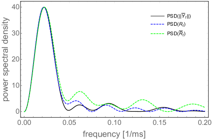
Figure 5: The norm of the process $\{\bar{\mathbf{Y}}_{t}\}$ (4.2), the process $\{R_{t}\}_{t}$ (4.3), and the process $\{\bar{R}_{t}\}_{t}$ (4.4) with the chosen parameters of system, $\sigma_{0}=0.01$ and the same starting point $\|Q^{-1}\bar{\mathbf{X}}_{0}\|$ are compared by using the power spectral density. Their spectrum densities are well approximated.

Firing mechanism

A spike in Eq. (3.1) occurs when there is a transition of a random trajectory from the vicinity of the stable fixed point $\mathbf{X}_{e}=(v_{e},w_{e})$ located on the left stable part of $\mathcal{C}_{0}$ to its right stable part and back to the vicinity of $\mathbf{X}_{e}$. This spike happens almost surely when a random trajectory with the starting point $\mathbf{X}_{0}$ in the vicinity of $\mathbf{X}_{e}$ crosses the threshold line $v=0$. From the phase space of Eq. (3.1) (see Fig. 2), the probability of a spike increases as the starting point $\mathbf{X}_{0}$ moves farther away from $\mathbf{X}_{e}$.

In order to construct the firing mechanism of Eq. (4.3) matching that of Eq. (3.1), we will calculate the conditional probability that Eq. (3.1) fires given that the trajectory crosses the line $L=\{(v_{e},w):w\leq w_{e}\}$. Denote by $L_{i}=(v_{e},w_{e}-l_{i})$ with $l_{i}=i\delta=i\frac{|w_{e}+0.453|}{20}$ for $i=0,1,\ldots,34$, then the distance between the equilibrium and $L_{i}$ is $l_{i}$. The value $|w_{e}+0.453|$ can be considered as the distance between the fixed point $(v_{e},w_{e})$ and the separatrix (see also Fig. 1) along $L$. For a given pair ($\sigma_{0},l_{i}$), a short trajectory starting in $L_{i}$ was simulated from (3.1), it was recorded whether a spike occurred (crossing the threshold $v=0$) in the first cycle of the stochastic path around $(v_{e},w_{e})$. This was repeated 1000 times and we counted the ratio of the number of spikes, denoted by $\hat{p}(l_{i},\sigma_{0})$, which is an estimate for the conditional probability of firing $p(l,\sigma_{0})$. The estimation was, furthermore, repeated for $\sigma_{0}=0.001,0.002,0.003,0.004,0.005,0.006,0.007,0.008,0.009,0.01,0.015$.

From the numerical simulation, for each $\sigma_{0}$, the estimate of the conditional probability is close to zero when we start in the immediate neighborhood of the stable fixed point and close to one when we start at the $L_{34}$, i.e., sufficiently far from the fixed point. Theses estimates appear to depend in a sigmoidal way on the distance from the stable fixed point. Therefore we assumed the conditional probability of firing to be of the form

(4.5) $$p(l)=\frac{1}{1+e^{\frac{a-l}{b}}}.$$

The parameters $a$ and $b$ then are estimated by using a non-linear regression from the above simulation data and are plotted in Fig. 6 for some different values of the noise amplitude $\sigma_{0}=0.003,0.005,0.007,0.009,0.01$, and $0.015$. We see that the family of estimates, $\hat{p}$, fits the fitted curve quite well for each value of $\sigma_{0}$. Regression estimates are reported in Table 1. Note that $p(a)=1/2$, i.e., $a$ is the distance along $L$ from $w_{e}$ at which the conditional probability of firing equals one half. For all values of $\sigma_{0}$, the estimate of $a$ is close to the distance along $L$ between $w_{e}$ and the separatrix, which equals $0.05$. In other words, the probability of firing, if the path starts at the intersection of $L$ with the sepametrix, is about $1/2$. The estimate of $b$ increases with respect to $\sigma_{0}$, and the conditional probability approaches a step function as the amplitude of the noise goes to zero. A step function would correspond to the firing being represented by a first passage time of a fixed threshold.

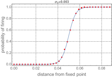
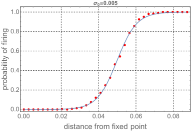
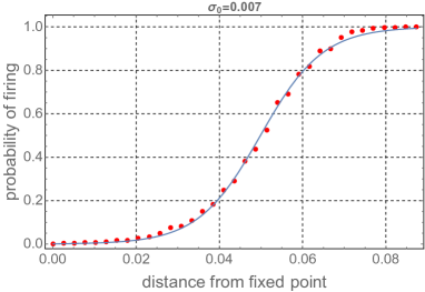
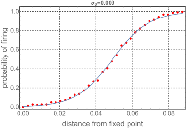
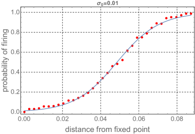
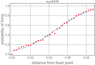
Figure 6: Conditional probability of spiking when crossing the line $L=\{(v_{e},w):w\leq w_{e}\}$ for different values of the noise amplitude $\sigma_{0}$. The red dots are individual nonparametric estimates and the blue curve are the fitted curves given by (4.5).

Table 1: Estimates of regression parameters for the conditional probability of firing in the original space and in the transformed coordinates based on the additive noise $\sigma_{0}$

$\sigma_{0}$	0.001	0.002	0.003	0.004	0.005	0.006	0.007	0.008	0.009	0.01	0.015
$a$	0.050161	0.050268	0.049946	0.049760	0.049816	0.050001	0.049862	0.049411	0.049078	0.048559	0.046142
$b$	0.001028	0.002099	0.003192	0.004310	0.005281	0.006459	0.007478	0.008844	0.009877	0.011068	0.017722
$a^{*}$	0.630282	0.631624	0.627576	0.625240	0.625935	0.628262	0.626516	0.620859	0.616673	0.610148	0.579777
$b^{*}$	0.012918	0.026372	0.040106	0.054158	0.066352	0.081158	0.093960	0.111127	0.124107	0.139075	0.222676

To simplify calculations we will work on the transformed coordinates $\bar{\mathbf{Y}}_{t}$. Then the distance $l$ between $(0,l)$ and $(0,0)$ in $\bar{\mathbf{X}}_{t}$ transforms to the distance

$$r=\Bigg{|}Q^{-1}\begin{pmatrix}0\\ l\end{pmatrix}\Bigg{|}=\sqrt{-\frac{m_{12}}{m_{21}\nu^{2}}}l.$$

and the conditional probability of firing Eq. (4.5) transforms to

(4.6) $$p(r)=\frac{1}{1+e^{\frac{a^{*}-r}{b^{*}}}}$$

where $a^{*}=\sqrt{-\frac{m_{12}}{m_{21}\nu^{2}}}a$ and $b^{*}=\sqrt{-\frac{m_{12}}{m_{21}\nu^{2}}}b$.

ISI distributions

The comparison of the original stochastic FHN model (3.1) and the two LIF models (4.3) and (4.4) can be performed by studying the ISI statistics. Namely, one first simulates the trajectories of the system (3.1) with starting points $\mathbf{X}_{0}$ close to the fixed point $\mathbf{X}_{e}$ until the first spiking time, and thereafter resets to the starting points. Due to Theorem 3.2, we can simplify the simulation by choosing the starting point at exactly $\mathbf{X}_{e}$. This was done 1000 times, and the time of the first firing was recorded. A histogram for this data is shown in Fig. 7. The ISI-distribution of Eq. (4.3) is computed as follows (the ISI-distribution of Eq. (4.4) is computed similarly). Let $\tau_{1}$ be the first firing time. We computed the density of the distribution of $\tau_{1}$ in terms of the conditional hazard rate [Ditlevsen and Greenwood, 2013],

$$\alpha(r,t)=\lim_{\Delta t\to 0}\frac{1}{\Delta t}P(t\leq\tau_{1}<t+\Delta t|\tau_{1}\geq t,R_{t}=r).$$

This function is the density of the conditional probability, given the position on $L$ is $r$ at time $t$, of a spike occurring in the next small time interval, given that it has not yet occurred.
Notice that the estimated conditional probability of firing (4.6) is calculated in one cycle of the process, which on average takes $2\pi/\nu$ time units. Therefore, we estimate the hazard rate as

(4.7) $$\alpha(r,t)=\alpha(r)=\frac{\nu}{2\pi}\frac{1}{1+e^{\frac{a^{*}-r}{b^{*}}}}.$$

On the other hand, from standard results from survival analysis, see e.g. [Aalen OO, 2] we know that the density of the firing time can be calculated as

(4.8) $$g(t)=\frac{d}{dt}P(\tau_{1}\leq t)=E\Bigg{(}\alpha(R_{t})e^{-\int_{0}^{t}\alpha(R_{s})ds}\Bigg{)}.$$

Due to the law of large numbers, for fixed $t$, we can numerically determine the density (4.8) up to any desired precision by choosing $n$ and $M$ large enough through the expression

$$g(t)\approx\frac{1}{M}\sum\limits_{m=1}^{M}\alpha(R^{(m)}_{t})e^{-\frac{t}{n}\sum\limits_{i=1}^{n}\frac{\alpha\big{(}R^{(m)}_{it/n}\big{)}+\alpha\big{(}R^{(m)}_{(i-1)t/n}\big{)}}{2}}.$$

Here ($R^{(m)}_{0},\ldots,R^{(m)}_{it/n},\ldots,R^{(m)}_{t})$ are $M$ realizations of $R_{it/n},i=0,1,\ldots,n$, and the integral has been approximated by the trapezoidal rule. The results are illustrated in Fig. 7 for $\sigma_{0}=0.01$, using $M=1000,n=10$. The estimated ISI distributions from our approximate LIF models (4.3) and (4.4) with the firing mechanism compare well with the estimated ISI histogram of FHN (3.1) reset to $0$ after firings.

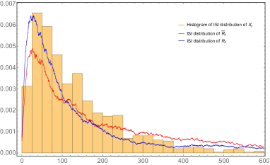
Figure 7: The estimated ISI distributions from our approximate LIF models (4.3) and (4.4) with the firing mechanism compare well with the estimated ISI histogram of FHN (3.1) reset to $0$ after firings. $\sigma_{0}=0.01,M=1000,n=10.$

5 Appendix

Proof 5.1 (Proof of Theorem 3.1).

We are going to prove that there exists a random pullback attractor for the general equation (3.2). Consider two cases:

• Additive noise: In this case, the proof follows similar steps as in [Garrido-Atienza et al., 2009]. We define $\mathbf{Y}_{t}=\mathbf{X}_{t}-\eta_{t}$ where $\eta_{t}$ is the unique stationary solution of

  $$d\eta_{t}=-\eta_{t}dt+(0,\sigma_{0})^{T}dB_{t}.$$

  System (3.2) is then tranformed to

  (5.1) $$\dot{\mathbf{Y}}_{t}=F(\mathbf{Y}_{t}+\eta_{t})+\eta_{t}.$$

  Observe that

  $$\frac{d}{dt}\|\mathbf{Y}_{t}\|^{2} = 2\langle\mathbf{Y}_{t},F(\mathbf{Y}_{t}+\eta_{t})-F(\eta_{t})\rangle+2\langle\mathbf{Y}_{t},F(\eta_{t})+\eta_{t}\rangle$$

  $$\leq 2(a-b\|\mathbf{Y}_{t}\|^{2})+b\|\mathbf{Y}_{t}\|^{2}+\frac{1}{b}\|F(\eta_{t})+\eta_{t}\|^{2}$$

  $$= 2a+\frac{1}{b}\|F(\eta_{t})+\eta_{t}\|^{2}-b\|\mathbf{Y}_{t}\|^{2}.$$

  Hence by the comparison principle, $\|\mathbf{Y}_{t}\|\leq R_{t}$ whenever $\|\mathbf{Y}_{0}\|^{2}\leq R_{0}$ where $R_{t}$ is the solution of

  (5.2) $$\dot{R}_{t}=2a+\frac{1}{b}\|F(\eta_{t})+\eta_{t}\|^{2}-bR_{t},$$

  which can be computed explicitly as

  $$R_{t}(\omega,R_{0})=e^{-bt}R_{0}+\int_{0}^{t}e^{-b(t-s)}\Big{[}2a+\frac{1}{b}\|F(\eta_{s})+\eta_{s}\|^{2}\Big{]}ds.$$

  It is then easy to check that the vector field in (5.1) satisfies the local Lipschitz property and the solution is bounded and thus of linear growth on any fixed $[0,T]$, see e.g. [Schenk-Hoppé, 1996]. Hence there exists a unique solution of (5.1) with initial condition, which also proves the existence and uniqueness of the solution of (3.2). The cocycle property (3.7) follows automatically from [Arnold, 1998, Chapter 2].

  A direct computation shows that there exists a random radius

  $$R^{*}(\omega)=\int_{-\infty}^{0}[2a+\frac{1}{b}\|F(\eta_{s})+\eta_{s}\|^{2}]e^{bs}ds,$$

  which is the stationary solution of (5.2), such that $\mathbf{X}_{t}(\omega,\mathbf{X}_{0})\in B(\eta_{t},R^{*}(\theta_{t}\omega))$ whenever $\mathbf{X}_{0}\in B(\eta_{0},R^{*}(\omega))$ by the comparison principle, and furthermore,

  $$\limsup\limits_{t\to\infty}\|\mathbf{Y}_{t}(\theta_{-t}\omega,\mathbf{Y}_{0})\|^{2}\leq\limsup\limits_{t\to\infty}R_{t}(\theta_{-t}\omega,R_{0})=R^{*}(\omega).$$

  Hence the random ball $B(\eta,R^{*})$ is a forward invariant pullback absorbing set of the random dynamical system generated by $\varphi(t,\omega)\mathbf{X}_{0}$ (3.2). By the classical theorem [Crauel et al., 1997], there exists the global random pullback attractor for (3.2).
  

• Multiplicative noise: In this case, we introduce the transformation

  (5.3) $$\mathbf{Y}_{t}=(v_{t},\bar{\omega}_{t})^{T}:=\begin{pmatrix}1&0\\ 0&e^{-\sigma_{0}z_{t}}\end{pmatrix}\mathbf{X}_{t}=T(z_{t})\mathbf{X}_{t}$$

  where $z_{t}$ is the unique stationary solution of the Ornstein-Uhlenbeck equation

  (5.4) $$dz_{t}=-z_{t}dt+dB_{t}.$$

  This transforms system (3.2) into a random differential equation.

  (5.5) $$\dot{v_{t}} = v_{t}-\frac{v_{t}^{3}}{3}-e^{\sigma_{0}z_{t}}\bar{\omega}_{t}+I$$

  $$\dot{\bar{\omega}}_{t} = e^{-\sigma_{0}z_{t}}\varepsilon v_{t}+(\sigma_{0}z_{t}-\varepsilon\beta)\bar{\omega}_{t}+\varepsilon\alpha e^{-\sigma_{0}z_{t}}.$$

  or equivalently,

  $$\dot{\mathbf{Y}}_{t}=G(z_{t},\mathbf{Y}_{t})$$

  where $G$ satisfies $G(z_{t},0)=(I,\varepsilon\alpha e^{-\sigma_{0}z_{t}})^{T}$ and

  $$\langle\mathbf{Y}_{1}-\mathbf{Y}_{2},G(z_{t},\mathbf{Y}_{1})-G(z_{t},\mathbf{Y}_{2})\rangle$$

  $$= (v_{1}-v_{2})^{2}\Big{[}1-\frac{1}{3}(v_{1}^{2}+v_{1}v_{2}+v_{2}^{2})\Big{]}+(\epsilon e^{-\sigma_{0}z_{t}}-e^{\sigma_{0}z_{t}})(v_{1}-v_{2})(\bar{w}_{1}-\bar{w}_{2})$$

  $$+(\sigma_{0}z_{t}-\epsilon\beta)(\bar{w}_{1}-\bar{w}_{2})^{2}$$

  $$\leq (v_{1}-v_{2})^{2}-\frac{1}{12}(v_{1}-v_{2})^{4}+\frac{1}{2\epsilon\beta}(\epsilon e^{-\sigma_{0}z_{t}}-e^{\sigma_{0}z_{t}})^{2}(v_{1}-v_{2})^{2}$$

  $$+(\sigma_{0}z_{t}-\frac{\epsilon\beta}{2})(\bar{w}_{1}-\bar{w}_{2})^{2}$$

  $$\leq -\frac{1}{12}(v_{1}-v_{2})^{4}+\Big{[}1+\frac{1}{2\epsilon\beta}(\epsilon e^{-\sigma_{0}z_{t}}-e^{\sigma_{0}z_{t}})^{2}-\sigma_{0}z_{t}+\frac{\epsilon\beta}{2}\Big{]}(v_{1}-v_{2})^{2}$$

  $$+(\sigma_{0}z_{t}-\frac{\epsilon\beta}{2})\|\mathbf{Y}_{1}-\mathbf{Y}_{2}\|^{2}$$

  $$\leq -\frac{1}{12}\Big{(}(v_{1}-v_{2})^{2}+6\Big{[}1+\frac{1}{2\epsilon\beta}(\epsilon e^{-\sigma_{0}z_{t}}-e^{\sigma_{0}z_{t}})^{2}-\sigma_{0}z_{t}+\frac{\epsilon\beta}{2}\Big{]}\Big{)}^{2}$$

  $$+3\Big{[}1+\frac{1}{2\epsilon\beta}(\epsilon e^{-\sigma_{0}z_{t}}-e^{\sigma_{0}z_{t}})^{2}-\sigma_{0}z_{t}+\frac{\epsilon\beta}{2}\Big{]}^{2}+(\sigma_{0}z_{t}-\frac{\epsilon\beta}{2})\|\mathbf{Y}_{1}-\mathbf{Y}_{2}\|^{2}$$

  $$\leq 3\Big{[}1+\frac{1}{2\epsilon\beta}(\epsilon e^{-\sigma_{0}z_{t}}-e^{\sigma_{0}z_{t}})^{2}-\sigma_{0}z_{t}+\frac{\epsilon\beta}{2}\Big{]}^{2}+(\sigma_{0}z_{t}-\frac{\epsilon\beta}{2})\|\mathbf{Y}_{1}-\mathbf{Y}_{2}\|^{2}.$$

  Thus,

  $$\frac{d}{dt}\|\mathbf{Y}_{t}\|^{2} = 2\langle\mathbf{Y}_{t}-0,G(z_{t},\mathbf{Y}_{t})-G(z_{t},0)\rangle+2\langle\mathbf{Y}_{t},G(z_{t},0)\rangle$$

  $$\leq 3\Big{[}1+\frac{1}{2\epsilon\beta}(\epsilon e^{-\sigma_{0}z_{t}}-e^{\sigma_{0}z_{t}})^{2}-\sigma_{0}z_{t}+\frac{\epsilon\beta}{2}\Big{]}^{2}+(\sigma_{0}z_{t}-\frac{\epsilon\beta}{2})\|\mathbf{Y}_{t}\|^{2}$$

  $$+2\langle\mathbf{Y}_{t},G(z_{t},0)\rangle$$

  $$\leq 3\Big{[}1+\frac{1}{2\epsilon\beta}(\epsilon e^{-\sigma_{0}z_{t}}-e^{\sigma_{0}z_{t}})^{2}-\sigma_{0}z_{t}+\frac{\epsilon\beta}{2}\Big{]}^{2}+\frac{4}{\varepsilon\beta}\|G(z_{t},0)\|^{2}$$

  $$+(\sigma_{0}z_{t}-\frac{\epsilon\beta}{4})\|\mathbf{Y}_{t}\|^{2}$$

  $$\leq 3\Big{[}1+\frac{1}{2\epsilon\beta}(\epsilon e^{-\sigma_{0}z_{t}}-e^{\sigma_{0}z_{t}})^{2}-\sigma_{0}z_{t}+\frac{\epsilon\beta}{2}\Big{]}^{2}+\frac{4}{\varepsilon\beta}\Big{[}I^{2}+\varepsilon^{2}\alpha^{2}e^{-2\sigma_{0}z_{t}}\Big{]}$$

  $$+(\sigma_{0}z_{t}-\frac{\epsilon\beta}{4})\|\mathbf{Y}_{t}\|^{2}$$

  $$\leq p(z_{t})+q(z_{t})\|\mathbf{Y}_{t}\|^{2}.$$

  Hence by the comparison principle, $\|\mathbf{Y}_{t}\|^{2}\leq R_{t}$ whenever $\|\mathbf{Y}_{0}\|^{2}\leq R_{0}$ where $R_{t}$ is the solution of

  (5.6) $$\dot{R}_{t}=p(z_{t})+q(z_{t})R_{t},$$

  which can be computed explicitly as

  $$R_{t}(\omega,R_{0})=e^{\int_{0}^{t}q(z_{u}(\omega))du}R_{0}+\int_{0}^{t}p(z_{s}(\omega))e^{\int_{s}^{t}q(z_{u}(\omega))du}ds.$$

  Using similar arguments as in the additive noise case, there exists a unique solution of (5.5) and (3.2). Also, the solution generates a random dynamical system.

  On the other hand, observe that by the Birkhorff ergodic theorem, there exists almost surely

  $$\lim\limits_{t\to-\infty}\frac{1}{t}\int_{t}^{0}q(z_{u})du=\lim\limits_{t\to-\infty}\frac{1}{t}\int_{t}^{0}q(z(\theta_{u}\omega))=E\Big{[}\sigma_{0}z(\cdot)-\frac{\varepsilon\beta}{4}\Big{]}=-\frac{\varepsilon\beta}{4}<0,$$

  therefore there exists a unique stationary solution of (5.6) which can be written in the form

  $$\bar{R}(\omega)=\int_{-\infty}^{0}p(z_{s}(\omega))e^{\int_{s}^{0}q(z_{u}(\omega))du}ds.$$

  Moreover, $\|\mathbf{Y}_{t}(\omega,\mathbf{Y}_{0})\|^{2}\leq\bar{R}(\theta_{t}\omega)$ whenever $\|\mathbf{Y}_{0}\|^{2}\leq\bar{R}(\omega)$ and

  $$\limsup\limits_{t\to\infty}\|\mathbf{Y}_{t}(\theta_{-t}\omega,\mathbf{Y}_{0})\|^{2}\leq\limsup\limits_{t\to\infty}R_{t}(\theta_{-t}\omega,R_{0})=\bar{R}(\omega).$$

  Hence, the ball $B(0,R(\omega))$ is actually forward invariant under the random dynamical system generated by (5.5) and is also a pullback absorbing set. Again by applying [Crauel et al., 1997], there exists a random attractor for (5.5). Due to the fact that $z_{t}$ is the stationary solution of (5.4), it is easy to see that the random linear transformation $T(z)$ given in (5.3) is tempered (see [Arnold, 1998, pp. 164, 386]), i.e.

  $$0\leq\lim\limits_{t\to\infty}\frac{1}{t}\log\|T(z_{t})\|=\lim\limits_{t\to\infty}\frac{1}{2t}\log(1+e^{-2\sigma_{0}z_{t}})\leq\lim\limits_{t\to\infty}\frac{1}{2t}(1+2\sigma_{0}|z_{t}|)=0.$$

  Therefore, it follows from [Imkeller and Schmalfuss, 2001] that systems (3.2) and (5.5) are conjugate under the tempered transformation (5.3), hence there exists also a random attractor for system (3.2).

Proof 5.2 (Proof of Theorem 3.2).

Observe that the matrix

$$DF(\mathbf{X}_{e})=\begin{pmatrix}m_{11}&m_{12}\\ m_{21}&m_{22}\end{pmatrix}$$

has two conjugate complex eigenvalues with negative real part

$$\lambda_{1,2}=\frac{1}{2}(1-v_{e}^{2}-\epsilon\beta)\pm\frac{i}{2}\sqrt{4\epsilon-(1-v_{e}^{2}+\epsilon\beta)^{2}}=-0.0730077\pm 0.31615i=-\mu\pm\nu i.$$

Hence by using the transformation $\mathbf{X}-\mathbf{X}_{e}=Q\mathbf{Y}$ and $\bar{X}=Q\bar{\mathbf{Y}}$ with

$$Q=\begin{pmatrix}-\nu&m_{11}+\mu\\ 0&m_{21}\end{pmatrix},$$

the equations (3.8) and (3.9) are transformed into the normal forms

(5.7) $$d\mathbf{Y}_{t} = \Big{[}Q^{-1}DF(\mathbf{X}_{e})Q\mathbf{Y}_{t}+Q^{-1}\bar{F}(Q\mathbf{Y}_{t})\Big{]}dt+Q^{-1}H(Q\mathbf{Y}_{t}+\mathbf{X}_{e})\circ dB_{t}$$

(5.8) $$= [A\mathbf{Y}_{t}+F_{1}(\mathbf{Y}_{t})]dt+Q^{-1}H(Q\mathbf{Y}_{t}+\mathbf{X}_{e})\circ dB_{t},$$

$$\mathbf{Y}_{0} = Q^{-1}(\mathbf{X}_{0}-\mathbf{X}_{e}),$$

and

(5.9) $$d{\bar{\mathbf{Y}}}_{t} = A\bar{\mathbf{Y}}_{t}dt+Q^{-1}H(Q\bar{\mathbf{Y}}_{t}+\mathbf{X}_{e})\circ dB_{t},$$

$$\bar{\mathbf{Y}}_{0} = Q^{-1}(\mathbf{X}_{0}-\mathbf{X}_{e}).$$

where

$$A=Q^{-1}DF(\mathbf{X}_{e})Q=\begin{pmatrix}-\mu&\nu\\ -\nu&-\mu\end{pmatrix};\qquad F_{1}(\mathbf{Y}):=Q^{-1}\bar{F}(Q\mathbf{Y}),$$

and

(5.10) $$\|F_{1}(\mathbf{Y})\|\leq\gamma(r)\|Q^{-1}\|\|Q\mathbf{Y}\|\leq\|Q^{-1}\|\gamma(r)r,\qquad\forall\|\mathbf{Y}\|\leq\frac{r}{\|Q\|}.$$

Define the difference $\mathbf{Z}_{t}:=\mathbf{Y}_{t}-\bar{\mathbf{Y}}_{t}$, then $\mathbf{Z}_{t}$ satisfies

$$d\mathbf{Z}_{t} = [A\mathbf{Z}_{t}+F_{1}(\mathbf{Y}_{t})]dt+B_{1}\mathbf{Z}_{t}\circ dB_{t}$$

$$= \Big{[}(A+\frac{1}{2}B_{1}^{T}B_{1})\mathbf{Z}_{t}+F_{1}(\mathbf{Y}_{t})\Big{]}dt+B_{1}\mathbf{Z}_{t}dB_{t},$$

where

$$B_{1}:=0\text{\ if\ }H(\mathbf{X})=(0,\sigma_{0})^{T}\quad\text{and}\quad B_{1}:=Q^{-1}BQ\text{\ if\ }H(\mathbf{X})=B\mathbf{X}.$$

We analyze these two cases separately.

• Additive noise: then the equation for $\mathbf{Z}_{t}$ becomes deterministic, hence

  $$\frac{d}{dt}\|\mathbf{Z}_{t\wedge\tau}\|^{2} = 2\Big{\langle}\mathbf{Z}_{t\wedge\tau},A\mathbf{Z}_{t\wedge\tau}+F_{1}(\mathbf{Y}_{t\wedge\tau})\Big{\rangle}$$

  $$\leq -2\mu\|\mathbf{Z}_{t\wedge\tau}\|^{2}+\mu\|\mathbf{Z}_{t\wedge\tau}\|^{2}+\frac{1}{\mu}\|F_{1}(\mathbf{Y}_{t\wedge\tau})\|^{2}$$

  $$\leq \frac{1}{\mu}\|Q^{-1}\|^{2}\gamma(r)^{2}r^{2}-\mu\|\mathbf{Z}_{t\wedge\tau}\|^{2}.$$

  Using the fact that $\mathbf{Z}_{0}=0$, it follows that

  $$\|\mathbf{Z}_{t\wedge\tau}\|^{2}\leq\frac{1}{\mu^{2}}\|Q^{-1}\|^{2}\gamma(r)^{2}r^{2}+e^{-\mu(t\wedge\tau)}\Big{(}\|\mathbf{Z}_{0}\|^{2}-\frac{1}{\mu^{2}}\|Q^{-1}\|^{2}\gamma(r)^{2}r^{2}\Big{)}.$$

  Therefore,

  $$\sup_{t\leq\tau}\|\mathbf{Z}_{t}\|\leq\frac{1}{\mu}\|Q^{-1}\|\gamma(r)r$$

  which proves (3.10) with $C=\frac{1}{\mu}\|Q\|\|Q^{-1}\|$.

• Multiplicative noise: By Ito’s formula for the stopping time,

  $$d\|\mathbf{Z}_{t\wedge\tau}\|^{2} = 2\Big{\langle}\mathbf{Z}_{t\wedge\tau},(A+\frac{1}{2}B_{1}^{T}B_{1})\mathbf{Z}_{t\wedge\tau}+F_{1}(\mathbf{Y}_{t\wedge\tau})\Big{\rangle}d(t\wedge\tau)+\|B_{1}\mathbf{Z}_{t\wedge\tau}\|^{2}d({t\wedge\tau})$$

  $$+2\langle\mathbf{Z}_{t\wedge\tau},B_{1}\mathbf{Z}_{t\wedge\tau}\rangle dB_{t\wedge\tau},$$

  hence taking the expectation on both sides and using (5.10) we have

  $$\frac{d}{dt}E\|\mathbf{Z}_{t\wedge\tau}\|^{2} \leq 2\Big{(}-\mu+\|B_{1}^{T}B_{1}\|\Big{)}E\|\mathbf{Z}_{t\wedge\tau}\|^{2}+2\|Q^{-1}\|\gamma(r)rE\|\mathbf{Z}_{t\wedge\tau}\|$$

  $$\leq (-\mu+2\|B_{1}^{T}B_{1}\|)E\|\mathbf{Z}_{t\wedge\tau}\|^{2}$$

  $$+\Big{[}-\mu\big{(}E\|\mathbf{Z}_{t\wedge\tau}\|\big{)}^{2}+2\|Q^{-1}\|\gamma(r)rE\|\mathbf{Z}_{t\wedge\tau}\|\Big{]}$$

  $$\leq (-\mu+2\|B_{1}^{T}B_{1}\|)E\|\mathbf{Z}_{t\wedge\tau}\|^{2}+\frac{1}{\mu}\|Q^{-1}\|^{2}\gamma(r)^{2}r^{2},$$

  where the last inequality follows from the Cauchy inequality. Since

  (5.11) $$\lambda=\mu-2\|B^{T}_{1}B_{1}\|>0,$$

  by noting that $\mathbf{Z}_{0}=0$, we get

  $$E\|\mathbf{Z}_{t\wedge\tau}\|^{2} \leq E\|\mathbf{Z}_{0\wedge\tau}\|^{2}e^{-\lambda(t\wedge\tau)}+\frac{1}{\mu}\|Q^{-1}\|^{2}\gamma(r)^{2}r^{2}\ \frac{1}{\lambda}\Big{[}1-e^{-\lambda(t\wedge\tau)}\Big{]}$$

  $$\leq \frac{1}{\mu}\frac{1}{\lambda}\|Q^{-1}\|^{2}\gamma(r)^{2}r^{2},$$

  which proves (3.11) by choosing $C:=\frac{1}{\mu}\frac{1}{\lambda}\|Q^{-1}\|^{2}\|Q\|^{2}$.

References

- [Aalen OO, 2] Aalen OO, Borgan Ø, G. H. (2). Survival and event history analysis. A process point of view. Springer, New York.
- [Arnold, 1998] Arnold, L. (1998). Random dynamical systems. Springer Monographs in Mathematics. Springer-Verlag, Berlin.
- [Baxendale and Greenwood, 2011] Baxendale, P. H. and Greenwood, P. E. (2011). Sustained oscillations for density dependent Markov processes. J. Math. Biol., 63(3):433–457.
- [Calvin and Stevens, 1967] Calvin, W. H. and Stevens, C. F. (1967). Synaptic noise as a source of variability in the interval between action potentials. Science, 155(3764):842–844.
- [Crauel et al., 1997] Crauel, H., Debussche, A., and Flandoli, F. (1997). Random attractors. J. Dynam. Differential Equations, 9(2):307–341.
- [Da Prato and Zabczyk, 1996] Da Prato, G. and Zabczyk, J. (1996). Ergodicity for infinite dimensional systems, volume 229. Cambridge University Press.
- [Ditlevsen and Greenwood, 2013] Ditlevsen, S. and Greenwood, P. (2013). The Morris–Lecar neuron model embeds a leaky integrate-and-fire model. Journal of Mathematical Biology, 67(2):239–259.
- [Fan and Yao, 2003] Fan, J. and Yao, Q. (2003). Spectral density estimation and its applications, chapter 7, pages 275–312. Springer New York, New York, NY.
- [FitzHugh, 1961] FitzHugh, R. (1961). Impulses and physiological states in theoretical models of nerve membrane. Biophysical Journal, 1(6):445–466.
- [Garrido-Atienza et al., 2009] Garrido-Atienza, M. J., Kloeden, P. E., and Neuenkirch, A. (2009). Discretization of stationary solutions of stochastic systems driven by fractional Brownian motion. Appl. Math. Optim., 60(2):151–172.
- [Gerstner and Kistler, 2002] Gerstner, W. and Kistler, W. M. (2002). Spiking neuron models. Cambridge University Press, Cambridge. Single neurons, populations, plasticity.
- [Hodgkin and Huxley, 1952] Hodgkin, A. L. and Huxley, A. F. (1952). A quantitative description of membrane current and its application to conduction and excitation in nerve. The Journal of Physiology, 117(4):500–544.
- [Imkeller and Schmalfuss, 2001] Imkeller, P. and Schmalfuss, B. (2001). The conjugacy of stochastic and random differential equations and the existence of global attractors. J. Dynam. Differential Equations, 13(2):215–249.
- [Izhikevich, 2007] Izhikevich, E. M. (2007). Dynamical systems in neuroscience: the geometry of excitability and bursting. Computational Neuroscience. MIT Press, Cambridge, MA.
- [Kuehn, 2015] Kuehn, C. (2015). Multiple time scale dynamics, volume 191 of Applied Mathematical Sciences. Springer, Cham.
- [Lansky and Ditlevsen, 2008] Lansky, P. and Ditlevsen, S. (2008). A review of the methods for signal estimation in stochastic diffusion leaky integrate-and-fire neuronal models. Biol. Cybernet., 99(4-5):253–262.
- [Morris and Lecar, 1981] Morris, C. and Lecar, H. (1981). Voltage oscillations in the barnacle giant muscle fiber. Biophysical Journal, 35(1):193–213.
- [Pfister et al., 2006] Pfister, J.-P., Toyoizumi, T., Barber, D., and Gerstner, W. (2006). Optimal spike-timing-dependent plasticity for precise action potential firing in supervised learning. Neural Comput., 18(6):1318–1348.
- [Schenk-Hoppé, 1996] Schenk-Hoppé, K. R. (1996). Deterministic and stochastic Duffing-van der Pol oscillators are non-explosive. Z. Angew. Math. Phys., 47(5):740–759.
- [White et al., 2000] White, J. A., Rubinstein, J. T., and Kay, A. R. (2000). Channel noise in neurons. Trends in Neurosciences, 23(3):131 – 137.
- [Yamakou, 2018] Yamakou, M. E. (2018). Weak-noise-induced phenomena in a slow-fast dynamical system. PhD thesis, Universität Leipzig.