Efficient Particle Smoothing for Bayesian Inference in Dynamic Survival Models

Abstract

This article proposes an efficient Bayesian inference for piecewise exponential hazard (PEH) models, which allow the effect of a covariate on the survival time to vary over time. The proposed inference methodology is based on a particle smoothing (PS) algorithm that depends on three particle filters. Efficient proposal (importance) distributions for the particle filters tailored to the nature of survival data and PEH models are developed using the Laplace approximation of the posterior distribution and linear Bayes theory. The algorithm is applied to both simulated and real data, and the results show that it generates an effective sample size that is more than two orders of magnitude larger than a state-of-the-art MCMC sampler for the same computing time, and scales well in high-dimensional and relatively large data.

Key words: Hazard function, Linear Bayes, particle filter, particle smoothing, piecewise exponential, Survival function.

Department of Statistics, Stockholm University
Parfait.Munezero@stat.su.se

1 Introduction

The standard model for analysing survival data is the proportional hazards model (Cox, 1972) which specifies the hazard function as a product of a baseline hazard (an unknown function of time, $t$) and a relative hazard (a function of the covariate vector, $\mathbf{x}$). This model assumes that the ratio of the hazards corresponding to two different covariate profiles is constant over time. However, in some situations the effect of the covariate may change over time, especially when the observation period is long.

Piecewise exponential hazard (PEH) models (Gamerman, 1991) allow the effect of the covariate to vary over time by assuming that both the baseline and relative hazard functions are piecewise constant over a set of disjoint and consecutive time intervals which partition the observation period. PEH models are special cases of the piecewise linear hazards models of Murray et al. (2016) and the more general P-spline hazard models proposed by Fahrmeir and Kneib (2011). Their key features are that the likelihood is tractable, and they are flexible enough to capture various shapes of the hazard function. Furthermore, they can be applied to both continuous survival time (Wagner, 2011) and discrete survival time (Fahrmeir and Wagenpfeil, 1996).

Current Bayesian inference procedures for PEH models make use of Markov Chain Monte Carlo (MCMC) methods. Hemming and Shaw (2002) build on the transformation of the prior process suggested by Gamerman (1998) to design a Metropolis-Hastings (MH) algorithm with random walk proposals. Fahrmeir and Kneib (2011) develop a MH algorithm with a multivariate Gaussian proposal defined using the score function and observed information matrix. Wagner (2011) develops a Gibbs sampler based on the data augmentation method of Frühwirth-Schnatter (1994) and proposes a variable selection scheme. The major drawback of these methods is that they are computationally expensive as they require many iterations to achieve convergence. Their convergence is hindered by the auto-correlation of the effect parameters induced by the random walk prior process.

The aim of this paper is to propose a fast and efficient alternative inference methodology for PEH models. The PS methodology is based on Sequential Monte Carlo (SMC) methods, commonly known as particle smoothing algorithms (Briers, Doucet, and Maskell, 2010; Fearnhead, Wyncoll, and Tawn, 2010). These algorithms are specifically designed to sample effectively from state-space models, of which PEH models is one instance. The main advantages of PS algorithms are that: i) they require no functional approximation of the likelihood, ii) they break a multidimensional problem into sequences of smaller dimensional problems. This makes them computationally fast and highly efficient especially when the number of intervals partitioning the study period is relatively large.

To be more specific, I apply the PS algorithm of Fearnhead et al. (2010), which relies on three particle filtering approximations: a forward particle filter which propagates information forwards in time, a backward particle filter which propagates information backwards in time, and a particle filter which combines the former two particle filters. These algorithms require a proposal distribution (importance distribution) that is easy to sample from. The so called bootstrap particle filters propose particles (parameter draws) from the prior distribution. This approach is prone to high degeneracy of the particles because the proposal does not incorporate any evidence from data. The standard way of incorportating evidence from data in the proposal distribution relies on the second order Taylor series expension of the log likelihood (Fearnhead et al., 2010). However, this is not appropriate for the PEH models because the mode and the hessian of the likelihood are not finite for censored individuals.

The main contribution of this paper is an efficient class of proposal distributions specially adapted to the nature of survival data and PEH models. The proposal of the forward filter is designed using the Laplace approximation of the posterior distribution of the hazard function with respect to the linear predictor (the log of the hazard function) and the linear Bayes method of West et al. (1985). The proposal distributions of the other filters follow the linear Bayes theory. Thus, the proposed inference algorithm is referred to as the particle smoother with linear Bayes proposals (PSLiB). The PSLiB algorithm is straightforward to implement since one needs only the Laplace approximation of the posterior of hazard function, and it can be easily extended to the class of multi-parameter regression models for survival data (Burke and MacKenzie, 2017) which model the survival time parametrically with each distributional parameter allowed to depend a set of covariates. Here, the only requirements would be the Laplace approximation of the posterior distribution of the distributional parameters with respect to the linear predictors.

The proposed inference methodology is applied to both simulated and real data. The simulation study, presented in Section 4, aims at investigating the performance of PSLiB with respect to the dimension of the covariate vector, the size of the dataset, the proportion of censored observations in the data, and the length of the study period. Results show that PSLiB is highly efficient in high-dimensional data and fairly large data with many observations, and scales well computationally. However, the performance degrades as the number of covariates and the proportion of censored observations increase. Similar performance degradation with respect to the number of covariates in the model has been noted by Villani et al. (2012) in a different class of models. Further, the comparison of PSLiB and the auxiliary mixture sampler (AMS) of Wagner (2011) shows that PSLiB outperforms AMS in terms of both the effective sample size and the computation time.

The rest of the paper is organized as follows. The next section delineates the likelihood and prior for the dynamic survival model. Section 3 presents the proposed inference methodology and, in Section 4, the performance of PSLiB is assessed through simulated and observed data. Finally, some concluding remarks and suggestions for future research are provided in Section 5.

2 Dynamic survival model specification

Let $\tilde{T}$ denote a random variable representing the survival time, which is the time until an event of interest occurs. Usually the survival time is not observed for all individuals participating in the study: some individuals are lost before they have experienced the event or, for some, the study ends before they experience the event. Individuals whose survival time is not known are called (right) censored observations. Letting the random variable $C$ denote the censoring time, the observed survival time is represented by the random variable $T=\min(\tilde{T},C)$.

The hazard function describes the instantaneous rate at which the event occurs, and it can be linked to the covariate vector $\mathbf{x}$ in various ways. This paper considers the Cox-type (Cox, 1972) multiplicative hazard model

$$\lambda(t|\mathbf{x})=\lambda_{0}(t)\exp\left(\mathbf{x}^{\prime}\mathbf{\boldsymbol{\beta}}\left(t\right)\right),$$ (1)

where $\boldsymbol{\beta}\left(t\right)$ is a vector of time-varying regression coefficients which models the effect of the covariates on the hazard function. The survival function,

$$S\left(t|\mathbf{x}\right)=\exp\left(-\int_{0}^{t}\lambda(s|\mathbf{x})ds\right),$$ (2)

is the probability that an individual with profile $\mathbf{x}$ has not experienced the event by time $t$. Given observed data for $n$ individuals: the exposure time $t_{i}$, the censoring indicator $d_{i}$ ($d_{i}=0$ if censored, and $d_{i}=1$ if event occurs), and the covariate vector $\mathbf{x}_{i}$ (for $i=1,\cdots,n$), the likelihood function is expressed as

$$L\left(t_{1},\ldots,t_{n}|\mathbf{\boldsymbol{\beta}}\left(t\right)\right)=\prod_{i=1}^{n}\lambda\left(t_{i}|\mathbf{x}_{i}\right)^{d_{i}}S\left(t_{i}|\mathbf{x}_{i}\right).$$ (3)

This model can be factorized sequentially into temporal factors by assuming that the hazard function is piecewise constant, which results in the PEH model (Gamerman, 1991).

2.1 The piecewise exponential hazard model

The PEH model partitions time into consecutive disjoint intervals, $I_{j}=[\tau_{j-1},\tau_{j})$ (where $j=1,\cdots,J$ and $\tau_{0}=0<\tau_{1}<,\cdots,<\tau_{J}$), and assumes that the baseline hazard function is constant within each interval $I_{j}$ ; i.e. $\lambda_{0}(t)=\lambda_{0j}$, for $t\in I_{j}$ and $\lambda_{0j}>0$. Furthermore, it assumes that the vector of regression coeficients $\boldsymbol{\beta}\left(t\right)$ is piecewise constant; i.e $\boldsymbol{\beta}\left(t\right)=\boldsymbol{\beta}_{j}$ if $t\in I_{j}$. Therefore, the hazard function is represented by several constant parameters $\lambda_{1},\ldots,\lambda_{J}$, where each $\lambda_{j}$ is connected to the covariate information of an individual $i$ through the log link

$$\ln\lambda_{ij}=\mathbf{z}_{i}^{\prime}\mathbf{\boldsymbol{\beta}}_{j},$$ (4)

which allows the flexibility to capture different shapes of the hazard function across time. Here, $\mathbf{z}_{i}=(1,\mathbf{x}_{i}^{\prime})$ is the original covariate vector of length $P$ augmented with a column of $1$, $\mathbf{\boldsymbol{\beta}}_{j}=(\mathbf{\beta}_{0j},\mathbf{\beta}_{1j},\cdots,\mathbf{\beta}_{Pj})$ represents the vector of regression coefficients, where the intercept $\mathbf{\beta}_{0j}=\ln(\lambda_{0j})$ is the log of the baseline hazard.

Partitioning time into discrete intervals generates interval-based data. The survival time $t_{i}$ breaks into several exposure times $t_{ij}=\max(0,\min(t_{i}-\tau_{j-1},\tau_{j}-\tau_{j-1}))$ which define the amount of time an individual $i$ is exposed to the occurence of the event during the interval $I_{j}$. The exposure time is equal to the length of $I_{j}$ (if individual $i$ survived through this interval), or it is equal to $t_{i}-\tau_{j-1}$ (if individual $i$ experienced the event or is censored in the interval $I_{j}$), otherwise it is equal to zero. Furthermore, the event indicator expands into a vector of binary variables $d_{ij}=1$ if the event occurs in interval $I_{j}$, and $d_{ij}=0$ if the individual is censored in or survives through the interval $I_{j}$.

With the assumption that covariates enter per (4), the survival function for individual $i$ becomes

$$S\left(t_{i}|\boldsymbol{x}_{i}\right)=\exp\left(-\left[\sum_{j=1}^{h-1}\lambda_{ij}\left(\tau_{j}-\tau_{j-1}\right)\right]-\lambda_{ih}\left(t_{i}-\tau_{h-1}\right)\right),\,\textrm{if }\tau_{h-1}\leq t_{i}<\tau_{h},\,h\leq J,$$ (5)

and the likelihood function (3) can be factorized across the intervals:

$$L\left(\mathbf{t}_{1:J}|\boldsymbol{\beta}_{1:J}\right) = \prod_{j=1}^{J}L_{j}\left(\mathbf{t}_{j}|\boldsymbol{\beta}_{j}\right),$$ (6)

where

$$L_{j}\left(\mathbf{t}_{j}|\boldsymbol{\beta}_{j}\right) =\prod_{i=1}^{n_{j}}\lambda_{ij}^{d_{ij}}\exp\left(-\lambda_{ij}t_{ij}\right),$$

$\mathbf{t}_{j}$ is the vector of exposures for interval $I_{j}$, $\mathbf{t}_{1:J}=(\mathbf{t}_{1},\ldots,\mathbf{t}_{J})$, $\boldsymbol{\beta}_{1:J}=(\beta_{1},\ldots,\beta_{J})$, and $n_{j}$ is the number of individuals who experienced the event during interval $I_{j}$. For more details and justification of the likelihood given in (6), see Gamerman (1991).

Alternative likelihood expressions can be obtained via data augmentation (Wagner, 2011) or partial likelihood (Sargent, 1997) approaches. The data augmentation approach completes the censored exposure times (corresponding to $d_{ij}=0$) by a latent exponentially distributed residual time. Wagner (2011) approximates the log of the augmented survival times by a mixture of ten normal components with known mean and variance parameters, resulting in a dynamic linear model. This method is used in Section 4.1 as a benchmark for assessing the performance of the inference methodology proposed in this paper.

The PEH model relies on the method of partitioning the time into $J$ intervals. The partition can be based on the event times, placing $\tau_{j}$ at each observed event time (Gamerman, 1991), which may be computationally expensive especially when the number of events is large. Alternatively, intervals could be equidistant as in Hemming and Shaw (2002), or they could contain equal number of events per interval (in this way there are more intervals in areas where there is more information). The selection of the number of events per interval can be done using a model comparison measure such as the Watanabe-Akaike information criterion (WAIC) descibed in Section 3.2.

2.2 Prior specification

In order to complete the model specification, one needs to define the prior process for the regression coefficients. One of the simplest and most applied smoothing priors on $\mathbf{\boldsymbol{\beta}}_{j}$ is the random walk

$$\mathbf{\boldsymbol{\beta}}_{j}=\mathbf{\boldsymbol{\beta}}_{j-1}+\epsilon_{j},\,\,\,\,\,\,\epsilon_{j}\sim N\left(0,\mathbf{U}_{j}\right).$$ (7)

This process is adopted by Wagner (2011), Fahrmeir (1994) and Hemming and Shaw (2002), and is a special case of the more general first order random walk process for parameter evolution suggested by Gamerman (1991). Clearly, if $\mathbf{U}_{j}$ is a zero matrix then there is no change in the regression coefficients and the dynamic model reduces to the standard proportional hazards model. Otherwise, $\mathbf{\boldsymbol{\beta}}_{j}$ varies over time and larger values for the entries in $\mathbf{U}_{j}$ indicate higher variation in $\mathbf{\boldsymbol{\beta}}_{j}$.

In many applications,$\mathbf{U}_{j}$ is held constant (i.e, $\mathbf{U}_{j}=\mathbf{U}$) and is assumed an unknown parameter. For a diagonal $\mathbf{U}_{j}$, both lognormal (Hemming and Shaw, 2002) and inverse gamma (Sargent, 1997; Wagner, 2011) priors have been suggested for the diagonal components. For a full matrix $\mathbf{U}_{j}$, Gamerman (1998) assumes an inverse Wishart prior on $\mathbf{U}_{j}$. Alternatively, West et al. (1985) suggests a discounting procedure for approximating $\mathbf{U}_{j}$ in terms of a discount parameter $0<\phi<1$ that controls the amount of information transferred through intervals. Given the posterior variance $\boldsymbol{\Sigma}_{j-1}$ of the regression coefficients in the interval $I_{j-1}$, the discount factor approach approximates $\mathbf{U}_{j}=(\phi^{-1}-1)\boldsymbol{\Sigma}_{j-1}$. This allows the variance $\mathbf{U}_{j}$ to vary over time, which improves the capacity of the random walk process to adapt locally. It is also possible to assume a time-varying discount factor (see Das and Dey (2013)). However, in this paper, $\mathbf{U}_{j}$ is allowed to be a full matrix, $\phi$ is held constant and inference on $\phi$ is based on the WAIC described in Section 3.2.

3 Inference

This section describes the posterior distribution and the sequential Monte Carlo sampling procedure used to sample from the target posterior distribution,

$$p\left(\boldsymbol{\beta}_{1:J}|\mathbf{t}_{1:J}\right)\propto p\left(\mathbf{t}_{1}|\boldsymbol{\beta}_{1}\right)p\left(\boldsymbol{\beta}_{1}\right)\prod_{j=2}^{J}L_{j}\left(\mathbf{t}_{j}|\boldsymbol{\beta}_{j}\right)p\left(\boldsymbol{\beta}_{j}|\boldsymbol{\beta}_{j-1}\right),$$ (8)

where $p(\boldsymbol{\beta}_{j}|\boldsymbol{\beta}_{j-1})$ is defined by the expression (7). MCMC methods have been used in the literature to sample from (8). Hemming and Shaw (2002) reparametrize $\boldsymbol{\beta}_{j}$ in terms of the evolution noise $\epsilon_{j}$ in (7), and apply a Gibbs sampler with a random walk Metropolis Hastings step for each $\boldsymbol{\beta}_{j}$. Wagner (2011) designs a Gibbs sampler where the full path $\boldsymbol{\beta}_{1:J}$ is sampled in one move using the forward filtering backward sampling algorithm (Frühwirth-Schnatter, 1994).

Note that the likelihood in (6) and the random walk prior process (7) define a state space model with non-linear and non-Gaussian observation model (Gordon et al., 1993), which allows to apply SMC inference methods. Generally, SMC methods are specifically designed for filtering problems (Doucet et al., 2000) in state space models, where the main objective is to sample from $p(\boldsymbol{\beta}_{1:j}\text{|}\mathbf{t}_{1:j}),\,j=1,\ldots,J,$ sequentialy through lower-dimensional marginals, $p(\boldsymbol{\beta}_{j}\text{|\,}\mathbf{t}_{1:j})$, referred to as filtering distributions.

SMC methods for sampling from (8) sequentially through the smoothing distribution, $p(\boldsymbol{\beta}_{j}\text{|}\mathbf{t}_{1:J})$, are also available in the literature. The forward-backward smoother samples parameters from the filtering distribution and smooths them in a backward procedure (see Doucet et al., 2000 and references therein). On the other hand, the two-filter smoother (Briers et al., 2010) and its computationally cheaper variant (Fearnhead et al., 2010) combine samples from both a forward and a backward information filter. This paper builds on the algorithm of the two-filter smoothing suggested by Fearnhead et al. (2010) and the linear Bayes method (West et al., 1985) to design an efficient inference scheme for PEH models.

3.1 The two-filter smoother

The two-filter smothing recursion (Briers et al., 2010) reformulates the smoothing distribution as

$$p\left(\boldsymbol{\beta}_{j}\text{|\,}\mathbf{t}_{1:J}\right)\propto p\left(\boldsymbol{\beta}_{j}\text{|\,}\mathbf{t}_{1:j-1}\right)p\left(\mathbf{t}_{j:J}|\,\boldsymbol{\beta}_{j}\right),$$ (9)

where the first term on the right hand side,

$$p\left(\boldsymbol{\beta}_{j}|\mathbf{t}_{1:j-1}\right)=\int p\left(\boldsymbol{\beta}_{j}|\boldsymbol{\beta}_{j-1}\right)p\left(\boldsymbol{\beta}_{j-1}|\mathbf{t}_{1:j-1}\right)d\boldsymbol{\beta}_{j-1},$$ (10)

is the predictive prior recursion, and the second term,

$$p\left(\mathbf{t}_{j:J}|\,\boldsymbol{\beta}_{j}\right)=L_{j}\left(\mathbf{t}_{j}|\boldsymbol{\beta}_{j}\right)\int p\left(\mathbf{t}_{(j+1):J}|\,\boldsymbol{\beta}_{j+1}\right)p\left(\boldsymbol{\beta}_{j+1}|\boldsymbol{\beta}_{j}\right)d\boldsymbol{\beta}_{j+1},$$ (11)

is the likelihood recursion. Both the expressions (10) and (11) are computed recursively through two independent filters: i) the forward filter which estimates sequentially the filtering distribution $p(\boldsymbol{\beta}_{j-1}|\mathbf{t}_{1:j-1})$ forward in time, and ii) the backward filter which evaluates the likelihood recursion (11) by mirroring the forward filter sequentially backward in time.

The forward filter begins from $j=1$ with a predifined initial distribution $p(\boldsymbol{\beta}_{1})$, and then proceeds propagating information forward in time through the usual posterior update:

$$p\left(\boldsymbol{\beta}_{j}|\mathbf{t}_{1:j}\right)\propto L_{j}\left(\mathbf{t}_{j}|\boldsymbol{\beta}_{j}\right)p\left(\boldsymbol{\beta}_{j}|\mathbf{t}_{1:j-1}\right),\,j=2,\ldots,J.$$ (12)

On the other hand, the formulation of the backward filter is not straightforward. It turns out that (11) is not a density for $\boldsymbol{\beta}_{j}$ and hence the integral may not be finite. To mirror the forward filter and ensure that the integral in (11) is always finite, Briers et al. (2010) introduce an artificial prior $\gamma_{j}\left(\boldsymbol{\beta}_{j}\right)$, for $j=J,\ldots,1$, so that the backward recursion expression becomes an artificial posterior; i.e,

$$\tilde{p}\left(\beta_{j}|\mathbf{t}_{j:J}\right) \propto p\left(\mathbf{t}_{j:J}|\,\boldsymbol{\beta}_{j}\right)\gamma_{j}\left(\boldsymbol{\beta}_{j}\right)$$ (13)

$$\propto L_{j}\left(\mathbf{t}_{j}|\boldsymbol{\beta}_{j}\right)\gamma_{j}\left(\boldsymbol{\beta}_{j}\right)\int\frac{\tilde{p}\left(\boldsymbol{\beta}_{j+1}|\mathbf{t}_{(j+1):J}\right)}{\gamma_{j+1}\left(\boldsymbol{\beta}_{j+1}\right)}p\left(\boldsymbol{\beta}_{j+1}|\boldsymbol{\beta}_{j}\right)d\boldsymbol{\beta}_{j+1},$$

where the first term in the inner expression of the integral is simply the likelihood $p(\mathbf{t}_{(j+1):J}|\,\boldsymbol{\beta}_{j+1})$. The backward filter starts at $J$ with the prior distribution $\gamma_{J}\left(\boldsymbol{\beta}_{J}\right)$ and proceeds by evaluating (13) recursively backward in time, for $j=J-1,\ldots,1$ .

The smoothing distribution $p(\boldsymbol{\beta}_{j}|\mathbf{t}_{1:J})$ is therefore estimated by combining the forward filter standing at $j-1$ and the backward filter standing at $j+1$ (see Algorithm $1$). If the likelihood is Gaussian and linear then both filters are analytically tractable. Otherwise, some form of approximation such as the particle filter approach (Doucet et al., 2000; Arulampalam et al., 2002) is needed.

3.1.1 Particle filtering approximation

Particle filters provide a recursive procedure of approximating the forward filtering distribution (12) by an empirical distribution defined on a finite sample of points $\{\boldsymbol{\beta}_{j}^{k}\}_{k=1}^{K}$ (commonly known as particles) weighted by the probability masses $\{w_{j}^{k}\}_{k=1}^{K}$ (importance weights). Assuming that a sample of particles and their corresponding importance weights at $j-1$ are available, then the predictive prior (10) is approximated as

$$p\left(\boldsymbol{\beta}_{j}|t_{1:j-1}\right)\propto\sum_{k=1}^{K}p\left(\boldsymbol{\beta}_{j}|\boldsymbol{\beta}_{j-1}^{k}\right)w_{j-1}^{k}.$$ (14)

Similarly, the backward filtering distribution (13) is approximated empirically by a finite sample of particles $\{\tilde{\boldsymbol{\beta}}_{j}^{k}\}_{k=1}^{K}$ weighted by $\{\tilde{w}_{j}^{k}\}_{k=1}^{K}$, and if the backward filter stands at the time point $j+1$, then the likelihood (11) is approximated as

$$p\left(\mathbf{t}_{j:J}|\,\boldsymbol{\beta}_{j}\right)\propto L_{j}\left(\mathbf{t}_{j}|\boldsymbol{\beta}_{j}\right)\sum_{h=1}^{K}\frac{p\left(\tilde{\boldsymbol{\beta}}_{j+1}^{h}|\boldsymbol{\beta}_{j}\right)}{\gamma_{j+1}\left(\tilde{\boldsymbol{\beta}}_{j+1}^{h}\right)}\tilde{w}_{j+1}^{h}.$$ (15)

Therefore, realizations from the forward particle filter standing at the time point $j-1$ and the backward filter at $j+1$ can be combined to approximate the smoothing distribution (9) as

$$p\left(\boldsymbol{\beta}_{j}\text{|\,}\mathbf{t}_{1:J}\right)\propto\sum_{k=1}^{K}\sum_{h=1}^{K}p\left(\boldsymbol{\beta}_{j}|\boldsymbol{\beta}_{j-1}^{k}\right)L_{j}\left(\mathbf{t}_{j}|\boldsymbol{\beta}_{j}\right)\frac{p\left(\tilde{\boldsymbol{\beta}}_{j+1}^{h}|\boldsymbol{\beta}_{j}\right)}{\gamma_{j+1}\left(\tilde{\boldsymbol{\beta}}_{j+1}^{h}\right)}w_{j-1}^{k}\tilde{w}_{j+1}^{h}.$$ (16)

The posterior (16) requires estimates of the forward and backward importance weights. Using importance sampling (Gordon et al., 1993), the importance weights are computed recursively as the ratio of the filtering distribution and the proposal distribution $q$ (for the forward filter) and $\tilde{q}$ (for the backward filter). Considering the auxiliary particle filter (APF) of Pitt and Shephard (1999), particles are proposed from the mixture distribution,

$$q\left(\boldsymbol{\beta}_{j}|\mathbf{t}_{1:j}\right)=\sum_{k=1}^{K}\nu_{j}^{k}q\left(\boldsymbol{\beta}_{j}|\boldsymbol{\beta}_{j-1}^{k},\mathbf{t}_{j}\right),$$ (17)

for the forward filter, and

$$\tilde{q}\left(\tilde{\boldsymbol{\beta}}_{j}|\mathbf{t}_{j:J}\right)=\sum_{h=1}^{K}\tilde{\nu}_{j}^{h}\tilde{q}\left(\tilde{\boldsymbol{\beta}}_{j}|\tilde{\boldsymbol{\beta}}_{j+1}^{h},\mathbf{t}_{j}\right),$$ (18)

for the backward filter. Where $\left\{\nu_{j}^{h}\right\}_{h=1}^{K}$ and $\left\{\tilde{\nu}_{j}^{k}\right\}_{h=1}^{K}$ are some normalized mixture weights. To sample from these proposal distributions a mixture component $a_{k}$ (referred to as ancestor) of $q$ is selected with probability proportional to $\nu_{j}$ and then a particle $\boldsymbol{\beta}_{j}^{k}$ is proposed from $q(\boldsymbol{\beta}_{j}|\boldsymbol{\beta}_{j-1}^{a_{k}},\mathbf{t}_{j})$; a similar procedure is used for $\tilde{q}$. Therefore, setting $\nu_{j}^{k}\wasypropto L_{j}(\mathbf{t}_{j}\text{|$\boldsymbol{\beta}$}_{j-1}^{k})w_{j-1}^{k}$ (and similarly $\tilde{\nu}_{j}^{h}\wasypropto L_{j}(\mathbf{t}_{j}\text{|$\beta$}_{j+1}^{h})\tilde{w}_{j+1}^{h}$ for the backward filter) implies that one proposes only from ancestors that have high importance weights and high predictive density.

Given the ancestors $a_{k}$ and $\tilde{a}_{h}$ from the forward and backward filters respectively, the corresponding importance weights become,

$$w_{j}^{k} \wasypropto\frac{p\left(\boldsymbol{\beta}_{j}^{k}|\,\mathbf{t}_{1:j}\right)}{q\left(\boldsymbol{\beta}_{j}^{k}|\,\mathbf{t}_{1:j}\right)}=\frac{L_{j}\left(\mathbf{t}_{j}|\,\boldsymbol{\beta}_{j}^{k}\right)p\left(\boldsymbol{\beta}_{j}^{k}|\,\boldsymbol{\beta}_{j-1}^{a_{k}}\right)}{L_{j}\left(\mathbf{t}_{j}\text{|\,$\boldsymbol{\beta}$}_{j-1}^{k}\right)q\left(\boldsymbol{\beta}_{j}^{k}|\,\boldsymbol{\beta}_{j-1}^{a_{k}},\mathbf{t}_{j}\right)},$$

$$\tilde{w}_{j}^{h} \wasypropto\frac{\tilde{p}\left(\tilde{\boldsymbol{\beta}}_{j}^{h}|\,\mathbf{t}_{j:J}\right)}{\tilde{q}\left(\tilde{\boldsymbol{\beta}}_{j}^{h}|\,\mathbf{t}_{j:J}\right)}=\frac{L_{j}\left(\mathbf{t}_{j}|\,\tilde{\boldsymbol{\beta}}_{j}^{h}\right)p\left(\tilde{\boldsymbol{\beta}}_{j+1}^{\tilde{a}_{h}}|\,\tilde{\boldsymbol{\beta}}_{j}^{h}\right)\gamma_{j}\left(\tilde{\boldsymbol{\beta}}_{j}^{h}\right)}{L_{j}\left(\mathbf{t}_{j}|\,\tilde{\boldsymbol{\beta}}_{j+1}^{\tilde{a}_{h}}\right)\widetilde{q}\left(\tilde{\boldsymbol{\beta}}_{j}^{h}|\,\tilde{\boldsymbol{\beta}}_{j+1}^{\tilde{a}_{h}},\mathbf{t}_{j}\right)\gamma_{j+1}\left(\tilde{\boldsymbol{\beta}}_{j+1}^{\tilde{a}_{h}}\right)}.$$ (19)

Finally, it remains to find a way of combining the two filters at each time point $j$. Instead of evaluating the double mixture (16) which is computationally costly, Fearnhead et al. (2010) suggest running another particle filter that combines the samples from the forward and backward particle filters recursively. This approach relies on finding another proposal distribution $\bar{q}(\boldsymbol{\beta}_{j}|\boldsymbol{\beta}_{j-1}^{k},\mathbf{t}_{j},\tilde{\boldsymbol{\beta}}_{j+1}^{h})$ combining draws from the forward particle filter at the time point $j-1$ and the backward particle filter at $j+1$. New smoothing particles $\bar{\{\boldsymbol{\beta}_{j}}^{s}\}_{s=1}^{S}$are proposed from $\bar{q}$, and the corresponding smoothing importance weights

$$\bar{w}_{j}^{s} \propto\frac{p\left(\bar{\boldsymbol{\beta}_{j}}^{s}|\boldsymbol{\beta}_{j-1}^{k}\right)L_{j}\left(\mathbf{t}_{j}|\bar{\boldsymbol{\beta}_{j}}^{s}\right)p\left(\tilde{\boldsymbol{\beta}}_{j+1}^{h}|\,\bar{\boldsymbol{\beta}_{j}}^{s}\right)w_{j-1}^{k}\tilde{w}_{j+1}^{h}}{\bar{q}\left(\bar{\boldsymbol{\beta}}_{j}|\boldsymbol{\beta}_{j-1}^{k},\mathbf{t}_{j},\tilde{\boldsymbol{\beta}}_{j+1}^{h}\right)\nu_{j}^{k}\,\tilde{\nu}_{j}^{h}\,\gamma_{j+1}\left(\tilde{\boldsymbol{\beta}}_{j+1}^{h}\right)},\,s=1,\ldots S$$

$$\propto\frac{p\left(\bar{\boldsymbol{\beta}_{j}}^{s}|\boldsymbol{\beta}_{j-1}^{k}\right)L_{j}\left(\mathbf{t}_{j}|\bar{\boldsymbol{\beta}_{j}}^{s}\right)p\left(\tilde{\boldsymbol{\beta}}_{j+1}^{h}|\,\bar{\boldsymbol{\beta}_{j}}^{s}\right)}{L_{j}\left(\mathbf{t}_{j}\text{|\,$\boldsymbol{\beta}$}_{j-1}^{k}\right)\bar{q}\left(\bar{\boldsymbol{\beta}}_{j}|\boldsymbol{\beta}_{j-1}^{k},\mathbf{t}_{j},\tilde{\boldsymbol{\beta}}_{j+1}^{h}\right)L_{j}\left(\mathbf{t}_{j}|\,\tilde{\boldsymbol{\beta}}_{j+1}^{h}\right)\gamma_{j+1}\left(\tilde{\boldsymbol{\beta}}_{j+1}^{h}\right)},$$ (20)

approximate empirically the posterior distribution (16). The two-filter smoother algorithm of Fearnhead et al. (2010) can be summarized in the following steps:

1. Forward particle filter

initialization: Sample $\beta_{0}^{k}\sim p\left(\beta_{0}\right)$ and set $w_{0}^{k}\propto\frac{1}{K}$

for $j=1$ to $J$ do

       for $k=1$ to $K$ do

            

            sample $\boldsymbol{\beta}_{j}^{k}\sim q(\boldsymbol{\beta}_{j}|\mathbf{t}_{1:j})$ and compute $w_{j}^{k}$ from (19)

       end for

      

end for

2. Backward particle filter

initialization: Sample $\beta_{J}^{h}\sim\gamma_{J}\left(\beta_{J}\right)$ and set $w_{J}^{k}\propto\frac{1}{K}$

for $j=J-1$ to $1$ do

       for $h=1$ to $K$ do

            

            sample $\tilde{\boldsymbol{\beta}}_{j}^{h}\sim\tilde{q}(\boldsymbol{\beta}_{j}|\mathbf{t}_{j:J})$ and compute $\tilde{w}_{j}^{h}$ from (19)

       end for

      

end for

3. Smoothing step: Combining the two filters

for $j=1$ to $J$ do

       for $s=1$ to $S$ do

            

            sample $\bar{\boldsymbol{\beta}_{j}}^{s}\sim\bar{q}(\boldsymbol{\beta}_{j}|\boldsymbol{\beta}_{j-1}^{k},\mathbf{t}_{j},\tilde{\boldsymbol{\beta}}_{j+1}^{h})$ and compute $\bar{w}_{j}^{s}$ from (20)

       end for

      

end for

Output: $\{\bar{\boldsymbol{\beta}_{j}},\bar{w}_{j}\}_{j=1}^{J}$

Algorithm 1 The two-filter smoother

Here, there are two things to be noted. First, the sample size $S$ of the smoothing particles need not be equal to the sample size for the forward (and backward) filtering particles $K$. One can gain computation time by setting $K$ small and $S$ bigger than $K$. More specifically by setting $S=RK$ ( in the following section $R=2$ in all runs of PSLiB). Second, the smoothing weights depend on the artificial prior $\gamma_{j+1}$, which can be any distribution. In order to ensure that the particles from backward filter are sampled from the smoothing distribution, Fearnhead et al. (2010) suggest setting $\gamma_{j+1}(\boldsymbol{\beta}_{j+1})=p(\boldsymbol{\beta}_{j+1}|\mathbf{t}_{1:j})$.

Given the particles sampled at the time point $j$ and their corresponding importance weights, this prior can be represented by the mixture in (14); however, doing this induces extra computational costs. To avoid it, one can use the linear Bayes method of West et al. (1985) to approximate the mixture by a single Gaussian distribution (see Appendix A).

3.1.2 Proposal distribution based on linear Bayes method

The aim of this section is to delineate the proposal distributions $q$, $\tilde{q}$ and $\bar{q}$. Since the regression coefficients are continuous random variables, it is convinient to construct $q$ as a mixture of Gaussian component distributions

$$q(\boldsymbol{\beta}_{j}|\boldsymbol{\beta}_{j-1},\mathbf{t}_{j})\simeq N_{P+1}(\boldsymbol{\beta}_{j}|\mathbf{m}_{j},\mathbf{C}_{j}),$$ (21)

where $\mathbf{m}_{j}$ and $\mathbf{C}_{j}$ are respectively the mean and covariance matrix of the component distributions of the mixture (17), and $P$ the dimension of the covariate vector. The standard APF proposes particles from the random walk process (7), which means that $\mathbf{m}_{j}=\boldsymbol{\beta}_{j-1}$ and $\mathbf{C}_{j}=\mathbf{U}_{j}$. This choice is prone to high degeneracy since particles are proposed from the prior. In addition to that, the discount factor approach, which defines $\mathbf{U}_{j}=(\phi^{-1}-1)\boldsymbol{\Sigma}_{j-1}$, makes this proposal impractical as it will be hard to control the variance of the proposal. To obtain a better proposal distribution it is necessary to include evidence from the data; one way to do this, is to linearize the likelihood locally through a second order Tylor series expansion of the log likelihood (Fearnhead et al., 2010) w.r.t the linear predictor $\eta_{j}$ around the mode value of $\eta_{j}$. For the PEH model, the mode of the linear predictor for an individual $i$ is $\hat{\eta}_{ij}=\log(\frac{d_{ij}}{t_{ij}})$ and the hessian is $d_{ij}^{-1}$. Hence, this linearization is not guaranteed to work since the mode and the hessian are not always finite – both $d_{ij}$ and $t_{ij}$ can be zero.

One alternative to get around this issue would be to first update the parameter $\lambda_{j}$ (the index $i$ is omitted for notational simplicity) and then exploit the fact that $\boldsymbol{\beta}_{j}$ enters the likelihood through the linear predictor, $\boldsymbol{\eta}_{j}=\ln\lambda_{j}=\mathbf{z}^{\prime}\mathbf{\boldsymbol{\beta}}_{j}$. Since $\eta_{j}$ and $\boldsymbol{\beta}_{j}$ are connected deterministically, one needs the posterior estimates $E[\eta_{j}|\mathbf{t}_{j}]$ and $V[\eta_{j}|\mathbf{t}_{j}]$ to update the mean and variance of $q(\boldsymbol{\beta}_{j}|\boldsymbol{\beta}_{j-1},\mathbf{t}_{j})$ using the conditional expectations

$$\mathbf{m}_{j} =E_{\eta_{j}}\left[E\left[\boldsymbol{\beta}_{j}|\eta_{j},\boldsymbol{\beta}_{j-1},\mathbf{t}_{1:j-1}\right]|\mathbf{t}_{j}\right],$$

$$\mathbf{C}_{j} =E_{\eta_{j}}\left[V\left[\boldsymbol{\beta}_{j}|\eta_{j},\boldsymbol{\beta}_{j-1},\mathbf{t}_{1:j-1}\right]|\mathbf{t}_{j}\right]+$$

$$\,\,\,V_{\eta_{j}}\left[E\left[\boldsymbol{\beta}_{j}|\eta_{j},\boldsymbol{\beta}_{j-1},\mathbf{t}_{1:j-1}\right]|\mathbf{t}_{j}\right].$$ (22)

The inner expectation of (22) are computed from a joint (degenerate) prior of $\eta_{j}$ and $\boldsymbol{\beta}_{j}$,

$$\left(\begin{array}[]{c}\eta_{j}\\ \boldsymbol{\beta}_{j}\end{array}\right)|\boldsymbol{\beta}_{j-1},\mathbf{t}_{1:j-1}\sim N_{P+2}\left(\left(\begin{array}[]{c}\boldsymbol{\mathbf{z}}^{\prime}\boldsymbol{\beta}_{j-1}\\ \boldsymbol{\beta}_{j-1}\end{array}\right),\,\,\left[\begin{array}[]{cc}\boldsymbol{\mathbf{z}}^{\prime}\hat{\boldsymbol{U}}_{j}\boldsymbol{\mathbf{z}}&\boldsymbol{\mathbf{z}}^{\prime}\mathbf{\hat{U}}_{j}\\ \hat{\boldsymbol{U}}_{j}\boldsymbol{\mathbf{z}}&\hat{\mathbf{U}}_{j}\end{array}\right]\right).$$ (23)

This method is known as linear Bayes and was proposed by West et al. (1985), and is guaranteed to work as long as the posterior of $\lambda_{j}$ is twice differentiable with respect to $\eta_{j}$. For more details see Appendix B.1.

Similarly, particles from the backward and the smoothing filters are respectively proposed from

$$\tilde{q}\left(\boldsymbol{\beta}_{j}|\tilde{\boldsymbol{\beta}}_{j+1},\mathbf{t}_{j}\right) \simeq N\left(\tilde{\boldsymbol{m}}_{j},\,\tilde{\boldsymbol{C}}_{j}\right),$$

$$\bar{q}\left(\boldsymbol{\beta}_{j}|\boldsymbol{\beta}_{j-1},\mathbf{t}_{j},\tilde{\boldsymbol{\beta}}_{j+1}\right) \simeq N\left(\bar{\boldsymbol{m}}_{j},\,\bar{\boldsymbol{C}}_{j}\right),$$ (24)

where $\tilde{\boldsymbol{m}}_{j}=(1-\phi)\hat{\boldsymbol{\mu}}_{j}+\phi\tilde{\boldsymbol{\beta}}_{j+1}$, $\tilde{\boldsymbol{C}}_{j}=(1-\phi)\hat{\boldsymbol{\Sigma}}_{j}$, $\bar{\boldsymbol{m}}_{j}=(1-\phi)\boldsymbol{m}_{j}+\phi\tilde{\boldsymbol{\beta}}_{j+1}$ and $\boldsymbol{\bar{C}}_{j}=(1-\phi)\boldsymbol{C}_{j}$. $\hat{\boldsymbol{\mu}}_{j}$ and $\hat{\boldsymbol{\Sigma}}_{j}$ are defined in (28) and $\boldsymbol{m}_{j}$ and $\boldsymbol{C}_{j}$ are the moments of the proposal for the forward filter defined in (22); further details are provided in Appendix B.2.

3.2 Model comparison and prediction

The inference methodology developed here relies on three key model choices: i) the discount factor, ii) the interval partition and iii) the covariates used in the model. Inference for these elements is based on the Watanabe-Akaike information creterion (WAIC); see Gelman et al. (2014). The WAIC uses the posterior sample and an out-of-sample test set to estimate the log posterior predictive density with an adjustment for the effective number of parameters. Given an out-of-sample test set of size $n_{\textrm{test}}$

$$WAIC =\sum_{i=1}^{n_{\textrm{test}}}\log E_{\textrm{post}}\left[L\left(t_{i}^{*}|\boldsymbol{\beta}_{1:J}\right)\right]-V_{\textrm{post}}\left[\log L\left(t_{i}^{*}|\boldsymbol{\beta}_{1:J}\right)\right]$$ (25)

$$=\sum_{i=1}^{n_{\textrm{test}}}\left\{\log\left(E_{\textrm{post}}\left[L\left(t_{i}^{*}|\boldsymbol{\beta}_{1:J}\right)\right]\right)-E_{\textrm{post}}\left[\left(\log L\left(t_{i}^{*}|\boldsymbol{\beta}_{1:J}\right)-E_{\textrm{post}}\left[\log L\left(t_{i}^{*}|\boldsymbol{\beta}_{1:J}\right)\right]\right)^{2}\right]\right\}.$$

Given a sample of particles $\{\boldsymbol{\beta}_{1:J}^{k}\}_{k=1}^{K}$ from the smoothing posterior distribution and their corresponding smoothing importance weights, $\{\bar{w}_{J}^{k}\}_{k=1}^{K}$ (note that $\bar{w}_{J}$ are the weights for the complete paths $\boldsymbol{\beta}_{1:J}$), the expectations in (25) can be approximated as

$$E_{\textrm{post}}\left[g\left(t_{i}|\beta_{1:J}\right)\right]=\frac{\sum_{k=1}^{K}g\left(t_{i}|\beta_{1:J}^{k}\right)\bar{w}_{J}^{k}}{\sum_{k=1}^{K}\bar{w}_{J}^{k}},$$ (26)

where $g$ is any transformation of the likelihood function. Further, the prediction of the probability that an individual $i$ survives up to the time $t$ is approximated by the particle smoother as

$$\hat{S}\left(t|\mathbf{x}_{i}^{*}\right) =\frac{\sum_{k=1}^{K}\bar{w}_{J}^{k}\exp\left(-\left\{\sum_{j=1}^{h-1}\left(\tau_{j}-\tau_{j-1}\right)\exp\left(\mathbf{z}_{i}^{*}{}^{\prime}\boldsymbol{\beta}_{j}^{k}\right)\right\}-\left(t-\tau_{h-1}\right)\exp\left(\mathbf{z}_{i}^{*}{}^{\prime}\boldsymbol{\beta}_{h}^{k}\right)\right)}{\sum_{k=1}^{K}\bar{w}_{J}^{k}},$$ (27)

if $\tau_{h-1}\leq t_{i}<\tau_{h},\,h\leq J$.

4 Applications

4.1 Simulations

A simulation study is conducted in order to assess the performance of PSLiB in various senarios and compare it with the state-of-the-art MCMC aproach in Wagner (2011). The censoring indicators $d_{i}$ ($i=1,\ldots,n$) are simulated from a Bernoulli distribution with probability $1-p_{c}$ ($p_{c}$ being the proportion of censored observations), and the exposure times, $t_{i}$, are simulated from the following PEH models (using inverse sampling):

$$\lambda_{ij}=\exp\left(\beta_{j,0}+\mathbf{x}_{i}^{\prime}\boldsymbol{\beta}_{j}\right),\,\,j=1,\ldots,J$$

$$\boldsymbol{\beta}_{j}=\boldsymbol{\beta}_{j-1}+\boldsymbol{\epsilon}_{j},\,\,\boldsymbol{\epsilon}_{j}\sim N_{P}\left(0,\,0.25I_{P}\right)$$

$$\beta_{j,0}=-11+\log\left(j\right),\,\,\boldsymbol{\beta}_{0}=0,\,x_{i}\sim N\left(0,I_{P}\right),$$

where $\boldsymbol{\beta}_{j}=(\beta_{j,1},\ldots,\beta_{j,p})^{\prime}$ and $I_{p}$ is a $P\times P$ diagonal matrix.

The above data generating process (DGP) allows the flexibility of varying the number of parameters $P$, the sample size $n$, the proportion of the censored observations $p_{c}$ and the number of intervals $J$ partitioning the study period. In all simulations, the intervals are equidistant and have length equals to $20$ units of time.

The performance of the inference methodology is measured by the expected discrimination measure (EDM) between the density for the DGP, $f(t|\mathbf{x})$, and the predictive density $\hat{f}(t|\mathbf{x})$ of a given fitted model,

$$EDM\left(f,\hat{f}\right)=\int\left[\int_{0}^{t}\frac{f\left(u|\mathbf{x}\right)}{F\left(t|\mathbf{x}\right)}\log\left(\frac{\nicefrac{{f(u|\mathbf{x})}}{{F(t|\mathbf{x})}}}{\nicefrac{{\hat{f}(u|\mathbf{x})}}{{\hat{F}(u|\mathbf{x})}}}\right)du\right]p\left(\mathbf{x}\right)d\mathbf{x},$$

where $F(t|\mathbf{x})$ and $\hat{F}(t|\mathbf{x})$ are the cumulative distribution functions (computed at time $t$) for the DGP and the fitted model respectively, and $p(\mathbf{x})$ is the marginal distribution of the covariates. For PEH models $F(t|\mathbf{x})=1-S(t|\mathbf{x})$ where $S(t|\mathbf{x})$ is the survival function. The expression in the inner integral was proposed by Di Crescenzo and Longobardi (2004), and is referred to as the measure of discrimination between two past-life distributions. To compute EDM, the inner intregral is evaluated numerically using the trapezoidal rule and the outer integral is approximated by taking the average over an out-of-sample test set of size $500$ simulated from $p(\mathbf{x})$. A value of EDM close to zero indicates that the fitted model reconstructs the DGP very well.

4.1.1 Performance assessment of PSLiB

To assess the effect of censoring and the covariate dimension on the performance of PSLiB, datasets are simulated from different DGPs: the number of covariates $P=1,5,10$, and the proportion of censored observations $p_{c}=10\%,25\%,50\%$ (for each $P$). That is, in total there are nine DGPs, and for each DGP, $50$ datasets of size $n=2500$ and survival time length $J=26$ are simulated. Figure 1 diplays the boxplots of the EDM between the DGP models and their corresponding fitted models. Models are fitted using PSLiB with $K=2000$ particles. Experiments show that increasing $K$ does not improve the EDM values. Furthermore, a discount factor $0.3\leq\phi\leq 0.45$ yields relatively low EDM values with the lowest obtained in most cases when $\phi=0.45$ (results not shown). Therefore, in the following analyses $\phi$ is set to the latter value.

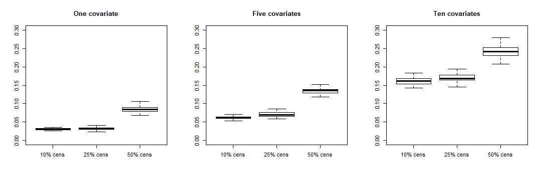
Figure 1: Evaluating the performance of PSLiB with respect to the dimension of the covariate vector and the proportion of censored observations. Results are based on $50$ simulated datasets of size $n=2500$ and $J=26$.

The EDM increases with both the number of variables and the proportion of censored observations. For models with one covariate, the average EDM is $0.030$, $0.032$ and $0.0850$ when the proportion of censored observations is $10\%$, $25\%$ and $50\%$ respectively. For models with five covariates, they increase to $0.061$, $0.071$ and $0.134$ respectively, and for models with ten covariates they increase even more to $0.181$, $0.172$, and $0.253$ respectively.

Table (1) presents the computation time of the PSLiB algorithm for different sample sizes, number of covariates, and number of intervals $J$. The effect of the number of particles is not investigated since Fearnhead et al. (2010) has shown that the particle smoother used here has a computational cost that increases linearly with the number of particles.

Table 1: CPU time (in minutes) for training models on simulated data with various sample sizes, number of covariates and length of the survival time. Results are averages over $50$ simulated datasets and $p_{c}=25\%$.

$\mathbf{n}$	One covariate			Five covariates			Ten covariates
	$\mathbf{J=6}$	$\mathbf{J=16}$	$\mathbf{J=26}$	$\mathbf{J=6}$	$\mathbf{J=16}$	$\mathbf{J=26}$	$\mathbf{J=6}$	$\mathbf{J=16}$	$\mathbf{J=26}$
$\mathbf{1000}$	$0.20$	$0.55$	$0.92$	$0.46$	$1.36$	$1.98$	$0.52$	$1.48$	$2.08$
$\mathbf{5000}$	$0.32$	$0.85$	$1.29$	$1.17$	$2.98$	$4.07$	$1.24$	$3.08$	$4.10$
$\mathbf{10000}$	$0.47$	$1.26$	$1.69$	$2.25$	$5.45$	$6.72$	$2.36$	$5.54$	$7.01$

CPU time increases from $P=1$ to $P=5$, but then remains roughly constant from $P=5$ to $P=10$. Therefore the number of covariates in the model does not influence significantly the running time of the algorithm. The effect of increasing $J$ is also modest: When $J=26$, $p=10$ and $n=10,000$ it takes $7$ CPU minutes, but when $n$ is increased to $50,000$ the computation time rises to $37$ CPU minutes and if $n$ is increased further to $100,000$ it takes$100$ CPU minutes to run the algorithm. Thus, for fixed covariate’s dimension, the computation time of PSLiB increases approximately linearly with the sample size.

4.1.2 Comparing PSLiB with AMS

This section compares the PSLiB and the MCMC algorithm in Wagner (2011) based on the number of effective sample size (ESS) of Carpenter et al. (1999),

$$ESS=\frac{\sigma_{j}^{2}}{E\left(\hat{\mu}_{j}-\mu_{j}\right)^{2}},$$

where $\hat{\mu}_{j}$ is the posterior estimate of the regression coefficients computed as in (28), and $\mu_{j}$ and $\sigma_{j}^{2}$ are respectively the true mean and variance of the regression coefficient, which following Carpenter et al. (1999), are approximated by taking averages of $\hat{\mu}_{j}$ and $\hat{\sigma}_{j}^{2}$ over $M$ independent runs of the algorithm.

To compare both the ESS and computation time for PSLiB and AMS, ESS per computation time (in CPU seconds) is used. The ESS is computed based on $M=100$ independent replications of the PSLiB and AMS runs on a dataset generated from a DGP with $P=1$, $J=26$ and $n=1000$. The same number of iterations ($5000$ MCMC iteration/particles) is set for both algorithms. The AMS model runs with the prior settings proposed by Wagner (2011).

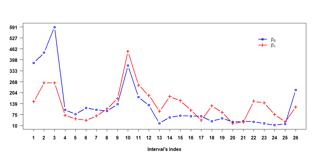
Figure 2: Comparing the PSLiB and AMS algorithms using the ratio of ESS/sec for PSLiB and AMS. The results are computated based on $100$ independent replications of each algorithm.

Figure 2 displays the ratio of the ESS/sec for PSLiB and AMS for all regression coefficients sampled in all $J$ intervals. It is clear form Figure 2 that PSLiB is more efficient as it generates, on average, an effective sample size that is more than two orders of magnitudes larger than AMS (the average ratio is $133$ for $\beta_{0}$, and $131$ for $\beta_{1}$). Comparing their computation time, PSLiB takes two minutes (CPU time) while AMS takes roughly $105$ minutes. The main reason for this difference is that PSLiB samples simultaneously all particles at each time point $j=1,\ldots,J$ and also it does not require the linearization of the likelihood in AMS.

4.2 Patients with Acute Myocardial Infraction (AMI).

In this section the PSLiB algorithm is applied to investigate the effect of different risk factors on the survival time of patients who were diagnosed with AMI. The dataset is a subset of the original data analyzed by Jensen et al. (1997), made available under the name “TRACE” in the R package “timereg” (Scheike, 2009). It contains survival times for $1878$ patients with AMI and six risk factors: age in years (age), heart pumping measured in ultrasound measurements (wmi), ventricular fibrillation indicator – vf ($1$: present, $0$: absent), clinical heart pump failure indicator – chf ($1$: present, $0$: absent), indicator of diabetes ($1$: present, $0$: absent), and sex ($1$: female, $0$: male). By the end of the follow-up time, $970$ of the $1878$ patients ($52\%$) died from myocardial infraction while the rest $908$ ($48\%$) were still alive or died from other causes and, hence, were considered as censored. The aim of the study is to estimate the effect of various risks on the survial time of patients.

The initial distribution, $p(\beta_{1})$, is set to the multivariate normal distribution with mean zero, and a diagonal covariance matrix where the variance of each covariate is set to $100$. The number of particles is set to $10000$, and the continuous covariates (mwi and age) are centered around their mean values. Since $970$ events are observed, it would be time consuming to partition the survivial time based on the event times. Time is instead partitioned into $J$ intervals, such that each interval contains $E$ events; a lower $E$ value of course increases the number of intervals and the computation time, but allows a more flexible form for the covariate effect. Note that although all intervals contain the same number of events, they need not be of the same length.

The WAIC is used to compare models with different discount factors $\phi$ and partitions of the survival time. The comparison is based on a randomly selected test set of size $470$ (roughly $20\%$ of the entire dataset) and the results are presented in Table 2.

Table 2: Comparing models fitted with different discount factors (in the rows) and different partitions of the study period (in columns) based on the WAIC.

$\phi$	$\mathbf{E=20}$	$\mathbf{E=30}$	$\mathbf{E=40}$	$\mathbf{E=50}$
$\mathbf{0.9}$	$2266.9$	$2427.7$	$2912.5$	$3497.1$
$\mathbf{0.8}$	$3775.7$	$3063.9$	$3256.1$	$2549.7$
$\mathbf{0.7}$	$3234.1$	$2856.3$	$2344.2$	$1683.8$
$\mathbf{0.6}$	$2139.4$	$1659.5$	$1420.8$	$1357.4$
$\mathbf{0.5}$	$1192.7$	$1184.2$	$1190.0$	$1186.8$
$\mathbf{0.4}$	$1278.3$	$1232.5$	$1214.9$	$1202.5$
$\mathbf{0.3}$	$1580.0$	$1294.2$	$1256.0$	$1242.6$

The lowest WAIC indicating the best model is observed when $\phi=0.5$ and $E=30$. Therefore, for further analysis, the discount factor and the number of events per interval are set respectively to the selected values. A partition of $30$ events per interval results into $32$ intervals; the initial intervals tend to be shorter than the latter intervals due to the decreasing risk set over time.

The WAIC is also used to select the risk factors to be included in further analysis of the AMI data. Setting the discount factor and the number of event per interval to the above-mentioned selected values, I fit models with all possible combination of the risk factors. The best model (WAIC= $1181$) contains only the risk factors: age, wmi, chf and vf. The posterior estimates for the parameters in the selected model as well as the predicted survival curves are presented in Figure 3. The survival curve are computed by setting the continuous variables (age and wmi) to their average values.

One can see that the risk factors wmi, vf and the chf have dynamic trends. The effect of the wmi increases in the first two and a half years then aftwerwards it starts declining slowly, but later on after six years it stabilizes around $-1.01$ (corresponding to a relative hazard of $0.36$). However, it is always negative indicating that the hazards of dying from AMI decreases with increasing wmi. The effect of chf drops considerably in the first month of diagnostics but later on it increases during next few months of the first year. After that, it starts declining slowly but always remains positive and converges to zero later on. The effect of vf is always positive as well but declines monotonically and converges towards zero after five years. On the other hand the effect of age is nearly static since its mean trajectory is more or less horizontal throughout the study period. The risk of dying from AMI increases roughly at a rate of $6\%$ times for each additional year on an individual’s age. Furthermore, the plot of the survival curves suggest that the group of patients with $chf=0$ and $vf=0$ have the highest survival curve, followed by the group with $chf=1$ and $vf=0$. The lowest survival curve corresponds to the group with $chf=1$ and $vf=1$. Thus, the risk of dying from AMI is much higher for patients with diagnosed with the heart pump failure (chf) compared to patients diagnosed with ventricular fibrillation (vf). The risk becomes even higher for patients who have both chf and vf.

Figure 3: Posterior mean trajectories of the log baseline hazards (intercept), the effect of the risk factors with their corresponding $95\%$ credible intervals (grey band), computed pointwise for each interval, and the fitted survival curves. The horizontal dashed line is a reference line at zero.

5 Concluding remarks

An efficient algorithm for posterior inference in piecewise exponential hazard models is proposed. The inference is based on a particle smoothing algorithm which applies three particle filters to sample from the posterior. This method requires designing efficient proposal distributions, which are developed by approximating the posterior distribution of the model parameters by a Gaussian distribution through a second order Taylor series expansion and applying the linear Bayes method of West et al. (1985).

The proposed inference methodology is shown to be fast and efficient for relatively large and high dimensional data and it generates an effective sample size that is more than two orders of magnitude higher than the MCMC sampler of Wagner (2011). Furthermore, it has been applied to make inference on the effect of risk factors of acute myocardial infraction and it turns out that the most important risk factors (based on WAIC) are: age, wmi, chf and vf , where the effect of all except the age vary with time.

Possible further extensions of the present work would be to generalize PSLiB to accomodates spatial covariates and/or time-varying covariates, or to allow higher order splines for the regression coefficients.

Acknowledgements: I would like to thank Mattias Villani, Gebrenegus Ghilagaber and Kevin Bruke for their constructive comments, and Helga Wagner for sharing the code for the auxiliary mixture sampler approach.

Appendix A The artificial prior distribution $\gamma_{j}$

The mean $\boldsymbol{\mu}_{j-1}$ and the covariance matrix $\boldsymbol{\Sigma}_{j-1}$ of the filtering distribution at time $j-1$ can be approximated from realizations of the forward particle filter by:

$$\hat{\boldsymbol{\mu}}_{j-1}=\frac{\sum_{k=1}^{K}\boldsymbol{\beta}_{j-1}^{k}w_{j-1}^{k}}{\sum_{k=1}^{K}w_{j-1}^{k}},\,\,\,\hat{\boldsymbol{\Sigma}}_{j-1}=\frac{\sum_{k=1}^{K}\left(\boldsymbol{\beta}_{j-1}^{k}-\hat{\boldsymbol{\mu}}_{j-1}\right)\left(\boldsymbol{\beta}_{j-1}^{k}-\hat{\boldsymbol{\mu}}_{j-1}\right)^{\prime}w_{j-1}^{k}}{\sum_{k=1}^{K}w_{j-1}^{k}}$$ (28)

Therefore, the mean and the variance of the mixture (14) are approximated respectively by $\hat{\boldsymbol{\mu}}_{j-1}$ and $\mathbf{\hat{R}}_{j}=\hat{\boldsymbol{\Sigma}}_{j-1}+\mathbf{\hat{U}}_{j}$, where $\mathbf{\hat{U}}_{j}=(\phi^{-1}-1)\hat{\boldsymbol{\Sigma}}_{j-1}$ is the approximation of the variance of the random walk prior process (7) . It follows that the artificial prior,

$$\gamma_{j}(\boldsymbol{\beta}_{j})\simeq N_{P+1}\left(\hat{\boldsymbol{\mu}}_{j-1},\frac{\hat{\boldsymbol{\Sigma}}_{j-1}}{\phi}\right).$$ (29)

Appendix B Details on the proposal distributions

B.1 The forward filter

Given the structure of the likelihood (6), the model parameter $\lambda_{ij}$ has a conjugate $\textrm{Gamma}(\alpha_{ij},\psi_{ij})$ prior distribution, which implies that the marginal posterior of $\lambda_{ij}$ is $\textrm{Gamma}(\alpha_{ij}+d_{ij},\psi_{ij}+t_{ij})$. Taking into account the Jacobian of the transformation $\eta_{ij}=\ln\lambda_{ij}$, it can be shown that

$$p\left(\eta_{ij}|\mathbf{t}_{1:j-1},\mathbf{t}_{1:i,j}\right)\propto\exp\left\{\eta_{ij}\left(\alpha_{ij}+d_{ij}\right)-\left(\psi_{ij}+t_{ij}\right)\exp\left\{\eta_{ij}\right\}\right\},$$ (30)

where $\mathbf{t}_{1:i,j}$ is the set of exposure times for the first $i$ individuals observed in the interval $I_{j}$. In order to apply the conditional expectations (22), a Laplace approximation of the posterior (30)

$$N\left(\left[\dfrac{\partial\ln p\left(\eta_{ij}|\mathbf{t}_{1:j-1},\mathbf{t}_{1:i,j}\right)}{\partial\eta_{ij}}\right]_{\eta_{ij}=\hat{\eta_{ij}}},\left[-\dfrac{\partial^{2}\ln p\left(\eta_{ij}|\mathbf{t}_{1:j-1},\mathbf{t}_{1:i,j}\right)}{\partial\eta_{ij}^{2}}\right]_{\eta_{ij}=\hat{\eta_{ij}}}^{-1}\right)$$

is required. Here $\hat{\eta_{ij}}$ is the mode value of the linear predictor. The first and second derivatives in (30) are given by :

$$\dfrac{\partial\ln p\left(\eta_{ij}|\mathbf{t}_{1:j-1},\mathbf{t}_{1:i,j}\right)}{\partial\eta_{ij}}=\alpha_{ij}+d_{ij}-\left(\psi_{ij}+t_{ij}\right)\exp\left\{\eta_{ij}\right\}$$

$$\dfrac{\partial^{2}\ln p\left(\eta_{ij}|\mathbf{t}_{1:j-1},\mathbf{t}_{1:i,j}\right)}{\partial\eta_{ij}^{2}}=-\left(\psi_{ij}+t_{ij}\right)\exp\left\{\eta_{ij}\right\}$$

From the first derivative, one can show that the mode lies at $\hat{\eta_{ij}}=\ln(\frac{\alpha_{ij}+d_{ij}}{\psi_{ij}+t_{ij}})$, which lead to the final expressions

$$E[\eta_{j}|\mathbf{t}_{j}]=\ln\left(\frac{\alpha_{ij}+d_{ij}}{\psi_{ij}+t_{ij}}\right),\thinspace\thinspace V[\eta_{j}|\mathbf{t}_{j}]=\frac{1}{\alpha_{ij}+d_{ij}}$$

The hyper-parameters $\alpha_{ij}$ and $\psi_{ij}$ are selected in order to match the true moments of the prior with the moments from the deterministic relationship $\eta_{ij}=\mathbf{z}_{i}^{\prime}\boldsymbol{\beta}_{j-1}$. This is accomplished by setting $\ln\alpha_{ij}-\ln\psi_{ij}=\mathbf{z}_{i}^{\prime}\boldsymbol{\beta}_{j-1}$ and $\alpha_{ij}^{-1}=\mathbf{z}_{i}^{\prime}\mathbf{U}_{j}\mathbf{z}_{i}$; hence $\psi_{ij}=\alpha_{ij}\exp\{-\mathbf{z}_{i}^{\prime}\boldsymbol{\beta}_{j-1}\}$. The moments of the proposal $q$ described in Section 3.1.2 are obtain from the recursive expressions (along $i=1,\ldots,n_{j}$),

$$\mathbf{m}_{ij} =\boldsymbol{\beta}_{j-1}+\frac{\mathbf{A}_{ij}}{Q_{ij}}\left(\ln\left(\frac{\alpha_{ij}+d_{ij}}{\psi_{ij}+t_{ij}}\right)-a_{ij}\right)$$

$$=\boldsymbol{\beta}_{j-1}+\frac{\mathbf{A}_{ij}}{Q_{ij}}\ln\frac{1+Q_{ij}d_{ij}}{1+t_{ij}Q_{ij}\exp\left\{a_{ij}\right\}}$$

$$\mathbf{C}_{ij} =\mathbf{U}_{j}-\frac{\mathbf{A}_{ij}\mathbf{A}_{ij}^{\prime}}{Q_{ij}}\left(1-\frac{1}{Q_{ij}\left(\alpha_{ij}+d_{ij}\right)}\right)$$

$$=\mathbf{U}_{j}-\mathbf{A}_{ij}\mathbf{A}_{ij}^{\prime}\left(\frac{d_{ij}}{1+d_{ij}Q_{ij}}\right)$$

where $a_{ij}=\mathbf{z}_{i}^{\prime}\boldsymbol{\beta}_{j-1}$ , $\mathbf{A}_{ij}=\mathbf{U}_{j}\mathbf{z}_{i}$, and $Q_{ij}=\mathbf{z}_{i}^{\prime}\mathbf{U}_{j}\mathbf{z}_{i}$. Starting with $i=1$, $\mathbf{m}_{1j}$ and $\mathbf{C}_{1j}$ are computed with $\boldsymbol{\beta}_{j-1}$ drawn from the sample of particles in the previous interval $I_{j-1}$ and then for $i+1$, $\boldsymbol{\beta}_{j-1}=\mathbf{m}_{i,j}$ and $\mathbf{U}_{j}=\mathbf{C}_{ij}$. Thus, $\mathbf{m}_{j}=\mathbf{m}_{n_{j},j}$ and $\mathbf{C}_{j}=\mathbf{C}_{n_{j},j}$.

B.2 The backward and smoothing filters

Given the weigthed particle sample from the forward particle filter, one can approximate $p(\boldsymbol{\beta}_{j}|\mathbf{z},\mathbf{t}_{1:j})$ by a Gaussian distribution with mean $\hat{\boldsymbol{\mu}}_{j}$ and covariance matrix $\hat{\boldsymbol{\Sigma}}_{j}$ defined in (28), the proposal $\tilde{q}$ is derived from the following joint distribution

$$\left.\left(\begin{array}[]{c}\boldsymbol{\beta}_{j}\\ \\ \boldsymbol{\beta}_{j+1}\end{array}\right)\right|\mathbf{t}_{j},\mathbf{d}_{j}\sim N\left(\left(\begin{array}[]{c}\hat{\boldsymbol{\mu}}_{j}\\ \\ \hat{\boldsymbol{\mu}}_{j}\end{array}\right),\,\left(\begin{array}[]{ccc}\hat{\boldsymbol{\Sigma}}_{j}&&\hat{\boldsymbol{\Sigma}}_{j}\\ \\ \hat{\boldsymbol{\Sigma}}_{j}&&\hat{R}_{j+1}\end{array}\right)\right),$$

where $\hat{R}_{j}$ is the variance of the prior $p(\boldsymbol{\beta}_{j+1}|\mathbf{t}_{j})$. The discount factor approach of West et al. (1985) assumes that $\hat{R}_{j+1}=\frac{\hat{\boldsymbol{\Sigma}}_{j}}{\phi}$ , $0<\phi<1$, which results in the conditional moments

$$E\left[\boldsymbol{\beta}_{j}|\boldsymbol{\beta}_{j+1},\mathbf{t}_{j}\right]=\hat{\boldsymbol{\mu}}_{j}+\phi\left(\boldsymbol{\beta}_{j+1}-\hat{\boldsymbol{\mu}}_{j}\right)=\phi\boldsymbol{\beta}_{j+1}+\left(1-\phi\right)\hat{\boldsymbol{\mu}}_{j}$$

$$V\left[\boldsymbol{\beta}_{j}|\boldsymbol{\beta}_{j+1},\mathbf{t}_{j}\right]=\hat{\boldsymbol{\Sigma}}_{j}-\phi\hat{\boldsymbol{\Sigma}}_{j}=\left(1-\phi\right)\hat{\boldsymbol{\Sigma}}_{j}$$

Since (as shown in the derivation of $q$ ) $\mathbf{m}_{j}$ and $\mathbf{C}_{j}$ correspond respectively to the mean and variance of $p(\boldsymbol{\beta}_{j}|\boldsymbol{\beta}_{j-1},\mathbf{t}_{j})$, therefore the moments of $\bar{q}$ are obtained by substituting $\mathbf{m}_{j}$ for $\hat{\boldsymbol{\mu}}_{j}$ and $\mathbf{C}_{j}$ for $\hat{\boldsymbol{\Sigma}}_{j}$ in the above expressions. Where, $\hat{\boldsymbol{\mu}}_{j}$ and $\hat{\boldsymbol{\Sigma}}_{j}$ are computed according to (29).

References

- Arulampalam et al. (2002) Arulampalam, M. S., S. Maskell, N. Gordon, and T. Clapp (2002). A tutorial on particle filters for online nonlinear/non-Gaussian Bayesian tracking. IEEE Transactions on signal processing 50(2), 174–188.
- Briers et al. (2010) Briers, M., A. Doucet, and S. Maskell (2010). Smoothing algorithms for state–space models. Annals of the Institute of Statistical Mathematics 62(1), 61–89.
- Burke and MacKenzie (2017) Burke, K. and G. MacKenzie (2017). Multi-parameter regression survival modeling: An alternative to proportional hazards. Biometrics 73(2), 678–686.
- Carpenter et al. (1999) Carpenter, J., P. Clifford, and P. Fearnhead (1999). Improved particle filter for nonlinear problems. IEE Proceedings-Radar, Sonar and Navigation 146(1), 2–7.
- Cox (1972) Cox, R. D. (1972). Regression models and life tables (with discussion). Journal of the Royal Statistical Society 34, 187–220.
- Das and Dey (2013) Das, S. and D. K. Dey (2013). On dynamic generalized linear models with applications. Methodology and Computing in Applied Probability, 1–15.
- Di Crescenzo and Longobardi (2004) Di Crescenzo, A. and M. Longobardi (2004). A measure of discrimination between past lifetime distributions. Statistics & probability letters 67(2), 173–182.
- Doucet et al. (2000) Doucet, A., S. Godsill, and C. Andrieu (2000). On sequential Monte Carlo sampling methods for Bayesian filtering. Statistics and computing 10(3), 197–208.
- Fahrmeir (1994) Fahrmeir, L. (1994). Dynamic modelling and penalized likelihood estimation for discrete time survival data. Biometrika 81(2), 317–330.
- Fahrmeir and Kneib (2011) Fahrmeir, L. and T. Kneib (2011). Bayesian smoothing and regression for longitudinal, spatial and event history data. Oxford University Press, New York..
- Fahrmeir and Wagenpfeil (1996) Fahrmeir, L. and S. Wagenpfeil (1996). Smoothing hazard functions and time-varying effects in discrete duration and competing risks models. Journal of the American Statistical Association 91(436), 1584–1594.
- Fearnhead et al. (2010) Fearnhead, P., D. Wyncoll, and J. Tawn (2010). A sequential smoothing algorithm with linear computational cost. Biometrika 97(2), 447–464.
- Frühwirth-Schnatter (1994) Frühwirth-Schnatter, S. (1994). Data augmentation and dynamic linear models. Journal of time series analysis 15(2), 183–202.
- Gamerman (1991) Gamerman, D. (1991). Dynamic Bayesian models for survival data. Applied Statistics, 63–79.
- Gamerman (1998) Gamerman, D. (1998). Markov Chain Monte Carlo for dynamic generalised linear models. Biometrika 85(1), 215–227.
- Gelman et al. (2014) Gelman, A., J. Hwang, and A. Vehtari (2014). Understanding predictive information criteria for Bayesian models. Statistics and Computing 24(6), 997–1016.
- Gordon et al. (1993) Gordon, N. J., D. J. Salmond, and A. F. Smith (1993). Novel approach to nonlinear/non-Gaussian Bayesian state estimation. In IEE Proceedings F (Radar and Signal Processing), Volume 140, pp. 107–113. IET.
- Hemming and Shaw (2002) Hemming, K. and J. Shaw (2002). A parametric dynamic survival model applied to breast cancer survival times. Journal of the Royal Statistical Society: Series C (Applied Statistics) 51(4), 421–435.
- Jensen et al. (1997) Jensen, G., C. Torp-Pedersen, P. Hildebrandt, L. Kober, F. Nielsen, T. Melchior, T. Joen, and P. Andersen (1997). Does in-hospital ventricular fibrillation affect prognosis after myocardial infarction? European Heart Journal 18(6), 919–924.
- Murray et al. (2016) Murray, T. A., B. P. Hobbs, D. J. Sargent, and B. P. Carlin (2016). Flexible bayesian survival modeling with semiparametric time-dependent and shape-restricted covariate effects. Bayesian analysis (Online) 11(2), 381.
- Pitt and Shephard (1999) Pitt, M. K. and N. Shephard (1999). Filtering via simulation: Auxiliary particle filters. Journal of the American Statistical Association 94(446), 590–599.
- Sargent (1997) Sargent, D. J. (1997). A flexible approach to time-varying coefficients in the Cox regression setting. Lifetime data analysis 3(1), 13–25.
- Scheike (2009) Scheike, T. (2009). Timereg: timereg package for flexible regression models for survival data. R package version 1.2-4.
- Villani et al. (2012) Villani, M., R. Kohn, and D. J. Nott (2012). Generalized smooth finite mixtures. Journal of Econometrics 171(2), 121–133.
- Wagner (2011) Wagner, H. (2011). Bayesian estimation and stochastic model specification search for dynamic survival models. Statistics and Computing 21(2), 231–246.
- West et al. (1985) West, M., P. J. Harrison, and H. S. Migon (1985). Dynamic generalized linear models and Bayesian forecasting. Journal of the American Statistical Association 80(389), 73–83.