Matrix valued inverse problems on graphs
with application to elastodynamic networks

Abstract

We consider the inverse problem of finding matrix valued edge or nodal quantities in a graph from measurements made at a few boundary nodes. This is a generalization of the problem of finding resistors in a resistor network from voltage and current measurements at a few nodes, but where the voltages and currents are vector valued. The measurements come from solving a series of Dirichlet problems, i.e. finding vector valued voltages at some interior nodes from voltages prescribed at the boundary nodes. We give conditions under which the Dirichlet problem admits a unique solution and study the degenerate case where the edge weights are rank deficient. Under mild conditions, the map that associates the matrix valued parameters to boundary data is analytic. This has practical consequences to iterative methods for solving the inverse problem numerically and to local uniqueness of the inverse problem. Our results allow for complex valued weights and give also explicit formulas for the Jacobian of the parameter to data map in terms of certain products of Dirichlet problem solutions. An application to inverse problems arising in elastodynamic networks (networks of springs, masses and dampers) is presented.

05C22, 05C50, 35R30.

1 Introduction

We study a class of inverse problems where the objective is to find matrix valued quantities defined on the edges or vertices (nodes) of a graph from measurements made at a few boundary nodes. The scalar case corresponds to the problem of finding resistors in a resistor network from electrical measurements made at a few nodes, see e.g. [14]. As in the scalar case, the vector potential at all the nodes can be found from its value at a few nodes by solving a Dirichlet problem which amounts to finding a vector potential satisfying a vector version of conservation of currents (Kirchhoff’s node law).

We present different inverse problems, where either the matrix valued weights on the edges or the vertices or even their eigenvalues are the unknown parameters that are sought after. All these inverse problems share a common structure that is given in Section 2. Any inverse problem that fits this mold has certain desirable properties: mainly the parameter to data map (i.e. the forward map) is analytic and its Jacobian can be computed in terms of products of internal states. Analyticity can be used to guarantee local uniqueness for such inverse problems, for almost any parameter within a region of interest provided the Jacobian is injective for one parameter (a generalization of the results in [6]). Moreover, we show that Newton’s method applied to such problems is very likely to produce valid steps. We study in detail the Dirichlet boundary value problem on graphs with matrix valued weights and give conditions under which the Dirichlet problem admits a unique solution (Sections 3 and 4). Our study includes cases where the matrix valued weights are rank deficient and uniqueness holds only up to a known subspace. Then in Sections 5 and 6 we formulate inverse problems with matrix valued weights and determine conditions under which they have the structure of Section 2. Some of the inverse problems we consider arise in elastodynamic networks, i.e. networks of springs, masses and dampers.

1.1 Related work

The discrete conductivity inverse problem consists in finding the resistors in a resistor network from voltage and current measurements made at a few nodes, assuming the underlying graph is known. For his problem, the uniqueness results in [13, 14, 10, 12, 11] apply to circular planar graphs and real conductivities. A different approach is taken in [9] where a monotonicity property inspired from the continuum [1] is used to show that if the conductivities satisfy a certain inequality then they can be uniquely determined from measurements, without specific assumptions on the underlying graph. The lack of uniqueness is shown for cylindrical graphs in [21]. For complex conductivities, a condition for “uniqueness almost everywhere” regardless of the underlying graph is given in [6]. Uniqueness almost everywhere means that the set of conductivities that have the same boundary data lie in a zero measure set and that the linearized problem is injective for almost all conductivities in some region.

Uniqueness for the discrete Schrödinger problem is considered in the real scalar case on circular planar graphs in [2, 3, 4]. This problem involves a resistor network with known underlying graph and resistors but where every node is connected to the ground (zero voltage) via a resistor with unknown resistance. These unknown resistors are a discrete version of the Schrödinger potential in the Schrödinger equation, and the goal is to find them from measurements made at a few nodes. A discrete Liouville identity [5] can be used to relate the discrete Schrödinger inverse problem for certain Schrödinger potentials to the discrete conductivity inverse problem, also on circular planar graphs. A condition guaranteeing uniqueness almost everywhere for complex valued potentials without an assumption on the graph is given in [6].

One of the consequences of the present study is a weak uniqueness result for matrix valued inverse problems on graphs. To the best of our knowledge there are no results for uniqueness of the inverse problem with matrix valued edge or node quantities other than the characterization and synthesis results for elastodynamic networks (discussed in more detail in Section 6) that are derived in [7, 18, 17]. These results solve an inverse problem for elastodynamic networks that assumes we are free to choose the graph topology. Indeed the constructions in [7, 18, 17] start from data generated by these networks (displacement to forces map) and give a network that reproduces this data. We emphasize that in the present study, the underlying graph is always assumed to be known.

2 Common structure

The discrete inverse problems we consider here share a common structure that we describe in section 2.1. Under the assumptions we make here, the linearization of the problem is readily available (section 2.2) and analyticity of the forward map is ensured. This has practical implications that are described in section 2.3.

2.1 An abstract inverse problem

We denote by $p\in\mathbb{C}^{m}$ the unknown parameter. As we see later in Sections 5 and 6, the parameter $p$ may represent a matrix valued quantity (or its eigenvalues) defined on the edges or nodes of a graph. The forward or parameter to data map associates to the parameter $p$ the matrix $\Lambda_{p}\in\mathbb{C}^{n\times n}$ (the data), provided the parameter $p$ belongs to an admissible set $R\subset\mathbb{C}^{m}$ of parameters. The inverse problem is to find $p$ from $\Lambda_{p}$. Furthermore, we assume that the discrete inverse problems we consider satisfy the following assumptions.

• Assumption 1. The parameter $p$ belongs to an open convex set $R\subset\mathbb{C}^{m}$ of admissible parameters. The forward map that to a parameter $p\in R$ associates the data $\Lambda_{p}$ is well defined for $p\in R$.

• Assumption 2. For all $f,g\in\mathbb{C}^{n}$ and $p_{1},p_{2}\in R$ the following boundary/interior identity holds:

  (1) $$f^{T}(\Lambda_{p_{1}}-\Lambda_{p_{2}})g=b(S_{p_{2}}g,S_{p_{1}}f)^{T}(p_{1}-p_{2}),$$

  where $b:\mathbb{C}^{\ell}\times\mathbb{C}^{\ell}\to\mathbb{C}^{m}$ is a bilinear mapping and $S_{p}\in\mathbb{C}^{\ell\times n}$ is a matrix defined for $p\in R$ that associates to a boundary condition $f\in\mathbb{C}^{n}$, an internal “state” $S_{p}f\in\mathbb{C}^{\ell}$.

• Assumption 3: Analyticity. The entries of $S_{p}$ are analytic functions of $p$ for $p\in R$.

Here by “analytic” we mean in the sense of analyticity of several complex variables, see e.g. [19]. For completeness, we recall in Appendix A all the results we use from the theory of functions of several complex variables. We note that the boundary/interior identity (1) is a discrete version of a similar identity that plays a key role in the Sylvester and Uhlmann [25] proof of uniqueness for the continuum Schrödinger inverse problem.

2.2 The product of solutions matrix and the Jacobian

For a discrete inverse problem satisfying assumptions 1–3, we define the following product of solutions matrix, which is the matrix valued function $W:R\times R\to\mathbb{C}^{m\times n^{2}}$ with columns given by

(2) $$[W(p_{1},p_{2})](:,i+(j-1)n)=b(S_{p_{1}}(:,i),S_{p_{2}}(:,j)),~{}i,j=1,\ldots,n.$$

The next lemma shows that the parameter to data map $\Lambda_{p}$ must be Fréchet differentiable (specialized versions of this lemma appear in [6, lemma 5.4 and 6.3]).

Lemma 2.1 (Linearization of discrete inverse problem).

Let $p\in R$. For sufficiently small $\delta p\in\mathbb{C}^{m}$, we have

(3) $$f^{T}\Lambda_{p+\delta p}g=f^{T}\Lambda_{p}g+b(S_{p}f,S_{p}g)^{T}\delta p+o(\delta p).$$

Proof 2.2.

Use the boundary/interior identity (1) with $p_{1}=p+\epsilon\delta p$ and $p_{2}=p$, for some scalar $\epsilon$. To conclude divide both sides by $\epsilon$ and take the limit as $\epsilon\to 0$. Notice that assumption 3 guarantees that $S_{p}$ is analytic in $p$, therefore we do have continuity of $S_{p}$ in $p$ and $S_{p+\epsilon\delta p}\to S_{p}$ as $\epsilon\to 0$.

A consequence of Lemma 2.1 is that $W(p,p)^{T}$ is a $n^{2}\times m$ matrix representation of the Jacobian matrix for the parameter to data map at parameter value $p$. From (2), the representation is associated to identifying the matrix $\Lambda_{p}\in\mathbb{C}^{n\times n}$ with the vector $\operatorname{vec}(\Lambda_{p})\in\mathbb{C}^{n^{2}}$, which is obtained by stacking the columns of $\Lambda_{p}$. Clearly the linearized inverse problem about $p$ is injective when $\mathcal{N}(W(p,p)^{T})=\{0\}$, i.e. when the product of solutions matrix $W(p,p)$ has full row rank, i.e. $\mathcal{R}(W(p,p))=\mathbb{C}^{m}$.

Another consequence of Lemma 2.1 is that the Jacobian of $\Lambda_{p}$ with respect to $p$ must be analytic for $p\in R$ (by assumption 3). Clearly the forward map $\Lambda_{p}$ must also be analytic for $p\in R$.

2.3 Analyticity and uniqueness almost everywhere

We look at the impact of analyticity on the uniqueness question:

If $p_{1},p_{2}\in\mathbb{C}^{m}$ are parameters with identical data $\Lambda_{p_{1}}=\Lambda_{p_{2}}$, can we conclude that $p_{1}=p_{2}$?

For inverse problems satisfying assumptions 1–3, we can only guarantee uniqueness in a weak sense that we call uniqueness almost everywhere (as in [6]). By this we mean that the linearized problem is injective for almost all parameters $p\in R$ and that the set of parameters having the data must be a zero measure set. Both properties follow readily from analyticity, as we see next.

Analyticity of the forward map $\Lambda_{p}$ readily gives uniqueness almost everywhere, meaning that the sets of parameters that have the same boundary data must be of zero measure. Indeed assume we can find $\rho_{1},\rho_{2}\in R^{2}$ such that $\Lambda_{\rho_{1}}\neq\Lambda_{\rho_{2}}$. Then we can consider the function $g:R\times R\to\mathbb{C}$ defined by $g(x,y)=[\Lambda_{x}-\Lambda_{y}]_{ij}$ for some $i,j\in 1,\ldots,n$. Clearly $g$ is analytic on $R^{2}$ and satisfies $g(\rho_{1},\rho_{2})\neq 0$. By analytic continuation, the set $\{(p_{1},p_{2})\in R\times R~{}|~{}g(p_{1},p_{2})=0\}$ must be a zero measure set. This is a much simpler way of reaching a result similar to in [6] and was suggested by Druskin [15].

Analyticity can also be used to deduce that if the Jacobian of the forward map is injective at a parameter $\rho\in R$, then it must be invertible at almost any other parameter $p\in R$. Indeed, Lemma 2.1 shows that the Jacobian at $p$ can be represented by the $n^{2}\times m$ matrix $W(p,p)^{T}$ defined in (2). If $W(\rho,\rho)^{T}$ is injective for a $\rho\in R$, then there is a $m\times m$ submatrix $[W(\rho,\rho)]_{:,\alpha}$ of $W(\rho,\rho)$ that is invertible, where $\alpha=(\alpha_{1},\ldots,\alpha_{m})\in\{1,\ldots,n^{2}\}^{m}$ is a multi-index used to represent the particular choice of columns. Thus the function $f:R\to\mathbb{C}$ defined by

(4) $$f(p)=\det[W(p,p)]_{:,\alpha}$$

is analytic for $p\in R$ and is such that $f(\rho)\neq 0$. By analytic continuation, the zero set of $f$ must be of measure zero. Thus the set of parameters for which the Jacobian is not injective must be a zero measure set.

Finally we note that if we can find a parameter $\rho$ for which the Jacobian $W(\rho,\rho)^{T}$ is injective, then we can use the constant rank theorem (see e.g. [24]) to show that there is a $\rho^{\prime}\in R$ in a neighborhood of $\rho$ such that $\Lambda_{\rho}\neq\Lambda_{\rho^{\prime}}$. Therefore the set of parameters that have the same data must be a zero measure set.

2.4 Applications of uniqueness almost everywhere

Uniqueness a.e. has several practical applications that are illustrated for the scalar discrete conductivity problem in [6]. We give an outline of these applications for completeness. The first application is a simple test to determine whether uniqueness a.e. holds for a particular discrete inverse problem and that may also indicate sensitivity to noise (section 2.4.1). Once we know uniqueness a.e. holds for a particular discrete inverse problem, we can guarantee that the situations in which Newton’s method with line search fails can be easily avoided (section 2.4.2). Naturally a statement about zero measure sets can be translated to a probabilistic setting (section 2.4.3).

2.4.1 A test for uniqueness almost everywhere

Recall from Lemma 2.1 that the Jacobian of the discrete inverse problem at a parameter $p$ can be easily computed as a products of solutions matrix (2) with $p\equiv p_{1}=p_{2}$. As discussed in section 2.3, if we can find a parameter $p\in R$ for which the Jacobian is injective, then uniqueness a.e. holds for the problem. A numerical test for uniqueness a.e. can be summarized as follows.

1. Pick a parameter $p\in R$.

2. Calculate the Jacobian $W(p,p)^{T}$ using (2).

3. Find the largest and smallest singular values $\sigma_{\max},\sigma_{\min}$ of $W(p,p)$.

4. If $\sigma_{\min}>\epsilon\sigma_{\max}$, where $\epsilon$ is a tolerance set a priori, then uniqueness a.e. holds.

We point out that if $\sigma_{\min}\leq\epsilon\sigma_{\max}$ it is not possible to distinguish between the two following scenarios: (a) uniqueness a.e. holds but $W(p,p)$ is not injective to precision $\epsilon$; or (b) uniqueness a.e. does not hold for the problem. Thus the test is inconclusive. However we know that scenario (a) is very unlikely because we would have had to pick $p$ on the zero measure subset of $R$ that contains all parameters for which the Jacobian is not injective. Thus the most likely outcome is (b). Finally we remark that other methods may be used instead of the Singular Value Decomposition (SVD) to find the rank of the Jacobian (e.g. the QR factorization). We prefer the SVD because the ratio $\sigma_{\max}/\sigma_{min}$ is the conditioning of the linear least squares problem associated with the linearization of the discrete inverse problem, and thus measures the sensitivity to noise of the linearization of the inverse problem about the parameter $p$.

2.4.2 Newton’s method

The discrete inverse problem of finding the parameter $p$ from the data $\Lambda_{p}$ is a non-linear system of equations that can be solved using Newton’s method (see e.g. [23]). Let us denote by $D\Lambda_{p}=W(p,p)^{T}$ the Jacobian of the Dirichlet to Neumann map about the parameter $p\in R$. For our particular problem we get the following.

Newton’s method
$p^{(0)}=$ given
for $k=0,1,2,\ldots$
	Find step $\delta p^{(k)}$ s.t. $D\Lambda_{p^{(k)}}\delta p^{(k)}=\operatorname{vec}(\Lambda_{p^{(k)}}-\Lambda_{p})$
	Choose step length $t_{k}>0$
	Update $p^{(k+1)}=p^{(k)}+t_{k}\delta p^{(k)}$

The first operation in the Newton iteration is to solve a linear problem for the step $\delta p^{(k)}$. This operation can fail either because $\operatorname{vec}(\Lambda_{p^{(k)}}-\Lambda_{p})\notin\mathcal{R}(D\Lambda_{p^{(k)}})$ or because $\mathcal{N}(D\Lambda_{p^{(k)}})\neq\{0\}$. A remedy to either of these situations is to solve the linear least squares system

(5) $$\min_{\delta p}\|D\Lambda_{p^{(k)}}\delta p-\operatorname{vec}(\Lambda_{p^{(k)}}-\Lambda_{p})\|_{2}^{2},$$

and pick $\delta p^{(k)}$ as the minimal norm solution to (5). If uniqueness a.e. holds for the problem at hand then clearly $D\Lambda_{p^{(k)}}$ is injective except on a zero measure set. Therefore we can expect the step in Newton’s method to be defined uniquely. Now assume we found a step. If we assume a particular form of analyticity for the entries of $S_{p}$ (in Assumption 3), then we can guarantee that there are only finitely many choices of the step length $t_{k}$ for which $D\Lambda_{p^{(k+1)}}$ is not injective. In the unlikely event one encounters one of such points, the step length $t_{k}$ can be reduced by a small amount to make $D\Lambda_{p^{(k+1)}}$ injective. This is a consequence of the following lemma, which is a generalization of the result for the scalar discrete conductivity inverse problem in [6, Corollary 5.7].

Lemma 2.3.

Consider a discrete inverse problem satisfying assumptions 1–3 and further assume that all entries of $S_{p}$ are rational functions of $p$ (of the form $P(p)/Q(p)$, where $P$ and $Q$ are polynomials). Let $p\in R$ and $\delta p\in\mathbb{C}^{m}$ and assume the Jacobian of $\Lambda_{p}$ at $p$ is injective. Then there are at most finitely many $t\in\mathbb{R}$ for which $p+t\delta p\in R$ and either

1. The Jacobian of $\Lambda_{p}$ at $p+t\delta p$ is not injective.

2. $\Lambda_{p+t\delta p}=\Lambda_{p}$.

Proof 2.4.

Since the Jacobian of $\Lambda_{p}$ is injective at $p\in R$, there is a multi-index $\alpha\in\{1,\ldots,n^{2}\}^{m}$ such that the function $f$ defined in (4) satisfies $f(p)\neq 0$. Since the admissible set is open and convex, there is an interval $[a,b]$ containing $0$ such that $t\in[a,b]\implies p+t\delta p\in R$. Since the entries of $S_{p}$ are rational functions of $p$ and $f$ is defined through a determinant we can see that the function $g(t)=f(p+t\delta p)$ is a rational function of $t$, i.e. it can be written in the form $g(t)=F(t)/G(t)$ where $F(t)$ and $G(t)$ are polynomials. Since $F(t)$ can only have finitely many zeroes, we conclude that there are only finitely many $t$ for which $g(t)=0$, or in other words, for which the Jacobian at $p+t\delta p$ is not injective. This proves (i). To prove (ii) we consider the function $h(t)=\det[W(p,p+t\delta p)]_{:,\alpha}$, with $\alpha$ being the same multi-index as in (i). The function $h$ is also a rational function in $t$ with finitely many zeroes. Notice that $h(t)\neq 0$ implies the matrix $W(p,p+t\delta p)$ has full row rank. Using the boundary/interior identity (1) we see that

$$\Lambda_{p+t\delta p}-\Lambda_{p}=tW(p,p+t\delta p)^{T}\delta p\neq 0$$

when $\delta p\neq 0$. Thus there are at most finitely many $t$ for which $\Lambda_{p+t\delta p}=\Lambda_{p}$, $p,p+\delta p\in R^{2}$ and $\delta p\neq 0$.

Remark 2.5.

The assumption on the entries of $S_{p}$ being rational functions of $p$ is satisfied by all the examples of discrete inverse problems on graphs that we consider in Sections 5 and 6. This is a simple consequence of the cofactor formula for the inverse of a matrix.

2.4.3 Probabilistic interpretation of uniqueness almost everywhere

The discussion in section 2.3 has a probabilistic flavor as was remarked for the scalar conductivity problem in [6]. To see this, consider a probability space $(\Omega,\mathcal{F},\mathbb{P})$ (i.e. a sample space $\Omega$, a set of events $\mathcal{F}$ and a probability measure $\mathbb{P}$) and consider a random variable $P:\Omega\to R\times R$ with distribution $\mu_{P}$ that we assume is absolutely continuous with respect to the Lebesgue measure on $\mathbb{C}^{m}\times\mathbb{C}^{m}$. Note that this assumption precludes the distribution $\mu_{P}$ from being supported on a set of Lebesgue measure zero in $R\times R$. We write $P\equiv(P_{1},P_{2})$ when we want to distinguish the components of $P$. If uniqueness a.e. holds for the discrete inverse problem at hand and $M\subset R\times R$ is a measurable set for which $\mathbb{P}\{P\in M\}>0$, then we must have

$$\mathbb{P}\{W(P_{1},P_{2})~{}\text{is injective}~{}|~{}P\in M\}=1.$$

To see this, remark that uniqueness a.e. guarantees that the set

$$Z=\{(p_{1},p_{2})\in M~{}|~{}W(p_{1},p_{2})~{}\text{is not injective}\}$$

is of measure zero. Since the distribution is absolutely continuous with respect to the Lebesgue measure, this also means $\mu_{P}(Z)=0$. Roughly speaking, if we choose two admissible parameters $p_{1},p_{2}$ at random, we have $W(p_{1},p_{2})$ injective almost surely. Thus we can tell $p_{1}$ and $p_{2}$ apart from the data $\Lambda_{p_{1}}$, $\Lambda_{p_{2}}$ almost surely.

A similar observation can be made regarding the injectivity of the Jacobian of the problem. Let $Q:\Omega\to R$ be a random variable with distribution $\mu_{Q}$ that is assumed to be absolutely continuous with respect to the Lebesgue measure. If uniqueness a.e. holds and $N\subset R$ is some measurable set with $\mathbb{P}\{Q\in N\}>0$, then we must have

$$\mathbb{P}\{\text{Jacobian at $Q$ is injective}~{}|~{}Q\in N\}=1.$$

3 The matrix valued conductivity and Schrödinger problems

3.1 Notation

We use the set theory notation $Y^{X}$ for the set of functions from $X$ to $Y$. For example $u\in(\mathbb{C}^{d})^{X}$ is a function $u:X\to\mathbb{C}^{d}$ that to some $x\in X$ associates $u(x)\in\mathbb{C}^{d}$. For some matrix $a\in\mathbb{C}^{d\times d}$ we write $a\succ 0$ (resp. $a\succeq 0$) to say that $a$ is positive definite (resp. positive semidefinite). When the same notation is used for $a\in(\mathbb{C}^{d\times d})^{X}$, the generalized inequality is understood componentwise, e.g. for $a\in(\mathbb{C}^{d\times d})^{X}$, $a\succ 0$ means $a(x)\succ 0$ for all $x\in X$. When we write $a\succ b$ (or $a\succeq b$) we mean $a-b\succ 0$ (or $a-b\succeq 0$). We use the notation $a=a^{\prime}+\jmath a^{\prime\prime}$, for the real $a^{\prime}=\text{Re}\,a$ and imaginary $a^{\prime\prime}=\text{Im}\,a$ parts of $a$.

By ordering a finite set $X$, it can be identified with $\{1,\ldots,|X|\}$, where $|X|$ is the cardinality of $X$. Thus $(\mathbb{C}^{d})^{X}$ can be identified with vectors in $\mathbb{C}^{d|X|}$. Similarly, upon fixing an ordering for another finite set $Y$, we can identify linear operators $(\mathbb{C}^{d})^{X}\to(\mathbb{C}^{d})^{Y}$ with matrices in $\mathbb{C}^{d|X|\times d|Y|}$.

For $A\in\mathbb{C}^{m\times n}$, we denote by $\operatorname{vec}(A)\in\mathbb{C}^{mn}$ the vector representation of the matrix $A$, i.e. the vector obtained by stacking the columns of $A$ in their natural ordering. Similarly for $a\in(\mathbb{C}^{d\times d})^{X}$, we denote by $\operatorname{vec}(a)\in\mathbb{C}^{d^{2}|X|}$, the vector representation of $a$, is the vector obtained by stacking the vector representations $\operatorname{vec}(a(x))$ of the matrices $a(x)$, for $x\in X$ in the predetermined ordering of $X$.

In addition to the usual matrix vector product, we also use a block-wise outer product ($\odot$), the Hadamard product ($\circledast$) and the Kronecker ($\otimes$) product. For $u,v\in(\mathbb{C}^{d})^{X}$, the (block-wise) outer product $u\odot v\in(\mathbb{C}^{d\times d})^{X}$ is

(6) $$(u\odot v)(x)=u(x)v(x)^{T},~{}x\in X.$$

The Hadamard or componentwise product of two vectors $a,b\in\mathbb{C}^{n}$ is denoted by $a\circledast b$ and it is given by $(a\circledast b)(i)=a(i)b(i)$, $i=1,\ldots n$. Finally the Kronecker product of two matrices $A\in\mathbb{C}^{n\times m}$ and $B\in\mathbb{C}^{p\times q}$ is the $np\times mq$ complex matrix $A\otimes B$ given by (see e.g. [20])

(7) $$A\otimes B=\begin{bmatrix}A_{11}B&\ldots&A_{1m}B\\ \vdots&&\vdots\\ A_{n1}B&\ldots&A_{nm}B\end{bmatrix}.$$

3.2 Discrete gradient, Laplacian and Schrödinger operators

We work with graphs $G=(V,E)$, where $V$ is the set of vertices or nodes (assumed finite) and $E$ is the set of edges $E\subset\{\{i,j\}|i,j\in V,i\neq j\}$. All graphs we consider are undirected and with no self-edges. We partition the nodes $V=B\cup I$ into a (nonempty) set $B$ of “boundary” nodes and a set $I$ of “interior” nodes.

By (discrete) conductivity $\sigma$ we mean a symmetric matrix valued function defined on the edges, i.e. $\sigma\in(\mathbb{C}^{d\times d})^{E}$. Here symmetric means $[\sigma(e)]^{T}=\sigma(e)$, for all $e\in E$. By (discrete) Schrödinger potential $q$ we mean a symmetric matrix valued nodal function i.e. $q\in(\mathbb{C}^{d\times d})^{V}$.

The $d-$dimensional discrete gradient is the linear operator $\nabla:(\mathbb{C}^{d})^{V}\to(\mathbb{C}^{d})^{E}$ defined for some $u\in(\mathbb{C}^{d})^{V}$ by

$$(\nabla u)(\{i,j\})=u(i)-u(j),~{}\{i,j\}\in E.$$

The discrete gradient assumes an edge orientation that is fixed a priori and that is irrelevant in the remainder of this paper.

The weighted graph Laplacian is the linear map $L_{\sigma}:(\mathbb{C}^{d})^{V}\to(\mathbb{C}^{d})^{V}$ defined by

(8) $$L_{\sigma}=\nabla^{T}\operatorname{diag}(\sigma)\nabla,$$

where we used the linear operator $\operatorname{diag}(\sigma):(\mathbb{C}^{d})^{E}\to(\mathbb{C}^{d})^{E}$, which is defined for some $v\in(\mathbb{C}^{d})^{E}$ by $(\operatorname{diag}(\sigma)v)(e)=\sigma(e)v(e)$, $e\in E$. Its matrix representation is a block diagonal matrix with the $\sigma(e)$ on its diagonal. The operator $\nabla^{T}:(\mathbb{C}^{d})^{E}\to(\mathbb{C}^{d})^{V}$ is the adjoint of the $d$-dimensional discrete gradient $\nabla$.

The discrete Schrödinger operator associated with a conductivity $\sigma$ and a Schrödinger potential $q$ is a block diagonal perturbation (with blocks of size $d\times d$) of the weighted graph Laplacian, i.e

$$L_{\sigma}+\operatorname{diag}(q).$$

Example 3.1.

We show how to use the matrix valued conductivities and Schrödinger potentials to view the Laplacian of a cylindrical graph $C=P_{k}\times G$ with scalar weights as a matrix valued Schrödinger operator on the graph $P_{k}$, a path with $k$ nodes with vertices $V(P_{k})=\{1,\ldots,k\}$ and edges $E(P_{k})=\{\{1,2\},\ldots,\{k-1,k\}\}$. Here $\times$ denotes the Cartesian product between graphs. Such cylindrical graphs arise e.g. in a finite difference discretization of the conductivity equation on a rectangle with a Cartesian grid, as illustrated in Fig. 1.

Let $s\in(0,\infty)^{E(C)}$ be a scalar conductivity on the cylindrical graph $C$. We view $s$ as a vector and split it into the sub-vectors $s^{j}\in(0,\infty)^{E(G)}$, $j=1,\ldots,k$ and $s^{j,j+1}\in(0,\infty)^{V(G)}$, $j=1,\ldots,k-1$. The sub-vector $s^{j}$ represents the scalar conductivity of the $j$-th copy of the graph $G$. The sub-vector $s^{j,j+1}$ corresponds to the conductivity linking layer $j$ to layer $j+1$. Define the matrix valued conductivity $\sigma\in(\mathbb{R}^{|V(G)|\times|V(G)|})^{E(P_{k})}$ by $\sigma(\{j,j+1\})=\operatorname{diag}s^{j,j+1}$, $j=1,\ldots,k-1$ and matrix valued Schrödinger potential $q\in(\mathbb{R}^{|V(G)|\times|V(G)|})^{V(P_{k})}$ by $q(j)=L_{s^{j}}$, i.e. the Laplacian of the graph induced by the vertices in the $j-$th copy of $G$, $j=1,\ldots,k$. Then with an appropriate ordering of the vertices we have

$$L_{\sigma}+\operatorname{diag}(q)=L_{s}.$$

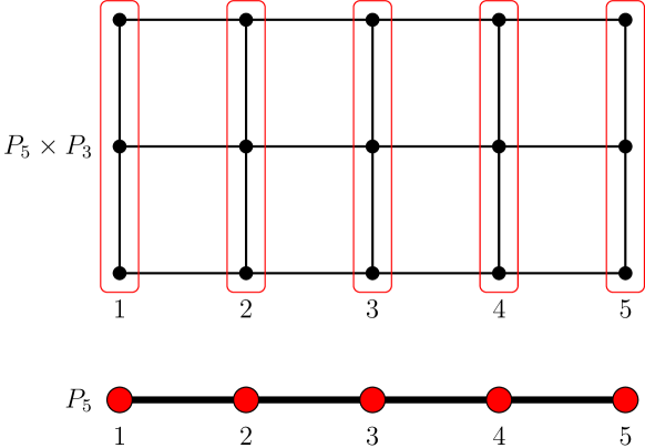
Figure 1: The Laplacian for a scalar conductivity on the cylindrical graph $C\equiv P_{5}\times P_{3}$ can be seen as a matrix valued Schrödinger operator on the graph $P_{5}$, as explained in Example 3.1. To fix ideas, $s^{4}\in\mathbb{R}^{2}$ represents the conductivities of $C$ within the $4-$th group in red and defines the matrix valued Schrödinger potential $q(4)$. The conductivity $s^{2,3}\in\mathbb{R}^{3}$ represents the conductivities of the 3 edges between the 2nd and 3rd group and is used to define the matrix valued conductivity $\sigma(\{2,3\})$.

3.3 The Dirichlet problem

For a conductivity $\sigma\in(\mathbb{C}^{d\times d})^{E}$ and a Schrödinger potential $q\in(\mathbb{C}^{d\times d})^{V}$, the $\sigma,q$ Dirichlet problem consists in finding $u\in(\mathbb{C}^{d})^{V}$ satisfying

(9) $$\left\{\begin{aligned} ((L_{\sigma}+\operatorname{diag}(q))u)_{I}&=0,~{}\text{and}\\ u_{B}&=g,\end{aligned}\right.$$

where $g\in(\mathbb{C}^{d})^{B}$ is the Dirichlet boundary condition. The Dirichlet to Neumann map, when it exists, is the linear mapping $\Lambda_{\sigma,q}:(\mathbb{C}^{d})^{B}\to(\mathbb{C}^{d})^{B}$ defined by

(10) $$\Lambda_{\sigma,q}g=((L_{\sigma}+\operatorname{diag}(q))u)_{B},$$

where $u$ solves the Dirichlet problem 9 with boundary condition $u_{B}=g\in(\mathbb{C}^{d})^{B}$. The Dirichlet to Neumann map is well defined e.g. when the solution to the Dirichlet problem is uniquely determined by the boundary condition. Conditions guaranteeing Dirichlet problem uniqueness are given in the next theorem.

Theorem 3.2.

The $\sigma,q$ Dirichlet problem on a connected graph with connected interior admits a unique solution when $\sigma\in(\mathbb{C}^{d\times d})^{E}$ and $q\in(\mathbb{C}^{d\times d})^{V}$ are symmetric and one of the two following conditions is satisfied.

1. $\sigma^{\prime}\succ 0$ and $q_{I}^{\prime}\succ-\lambda_{\min}\left({(L_{\sigma^{\prime}})_{II}}\right)$.

2. $q_{I}^{\prime}\succ 0$ and $(L_{\sigma^{\prime}})_{II}\succ-\lambda_{\min}(\operatorname{diag}(q_{I}^{\prime}))$.

In the previous theorem, $\lambda_{\min}(A)$ denotes the smallest eigenvalue of a real symmetric matrix $A$. When any of the conditions from Theorem 3.2 hold, the Dirichlet to Neumann map can be written as

(11) $$\Lambda_{\sigma,q}=L_{BB}+\operatorname{diag}(q_{B})-L_{BI}(L_{II}+\operatorname{diag}(q_{I}))^{-1}L_{IB},$$

where we dropped the subscript $\sigma$ in the blocks $(L_{\sigma})_{BB}$, $\ldots$ for clarity.

Unfortunately Theorem 3.2 and the expression 11 of the Dirichlet to Neumann map do not apply to one the main applications of our results: static spring networks. As we see in more detail in section 6.1, the linearization of Hooke’s law we use allows for non-physical floppy modes, i.e. non-zero displacements that can be made with zero forces. A generalization of the static spring network problem is to consider symmetric conductivities with $\sigma\succeq 0$. In this situation, floppy modes may also arise if there are edges $e$ for which $\sigma(e)$ has a non-trivial nullspace. They can be defined as follows.

Definition 3.3.

A non-zero $z\in\mathbb{C}^{V}$, is said to be a floppy mode for a symmetric conductivity $\sigma\in(\mathbb{C}^{d\times d})^{E}$ with $\sigma\succeq 0$ if $z$ solves the equation

(12) $$\left\{\begin{aligned} (L_{\sigma}z)_{I}&=0,\\ z_{B}&=0.\end{aligned}\right.$$

If $z$ is a floppy mode, then the solution to the $\sigma,0$ Dirichlet problem cannot be unique. Indeed if $u$ is a solution to the $\sigma,0$ Dirichlet problem, them so is $u+\alpha z$ for any scalar $\alpha$. The following theorem shows that even in the degenerate case $\sigma\succeq 0$, $q=0$, there are situations where the Dirichlet problem admits a solution that is unique up to floppy modes.

Theorem 3.4.

The $\sigma,0$ Dirichlet problem on a connected graph with connected interior and $\sigma(e)\neq 0$ for all $e\in E$, admits a unique solution up to floppy modes when any of the two following conditions hold.

1. $\sigma^{\prime}\succeq 0$ and $\sigma^{\prime\prime}=0$.

2. $\sigma^{\prime}\succeq 0$, and for each $e\in E$, $\sigma^{\prime\prime}(e)$ commutes with $\sigma^{\prime}(e)$ with nullspaces satisfying the inclusion $\mathcal{N}(\sigma^{\prime}(e))\subset\mathcal{N}(\sigma^{\prime\prime}(e))$.

The next lemma shows that the Dirichlet to Neumann map is well defined in the degenerate cases considered in Theorem 3.4.

Lemma 3.5.

Under the hypothesis of Theorem 3.4, the Dirichlet to Neumann map is

(13) $$\Lambda_{\sigma,0}=L_{BB}-L_{BI}Q(Q^{T}L_{II}Q)^{-1}Q^{T}L_{IB},$$

where for clarity we dropped the subscript $\sigma$ in the blocks $(L_{\sigma})_{BB}$ etc. The matrix $Q$ is real with orthonormal columns ($Q^{T}Q=\mathbb{I}$) and satisfies $\mathcal{R}(Q)=\mathcal{R}(L_{II})$. Moreover $Q$ depends only on the eigenvectors of $\sigma^{\prime}(e)$ associated with non-zero eigenvalues, for $e\in E$.

The proofs of Theorems 3.2, 3.4 and 3.5 are deferred to Section 4.

Remark 3.6 (Discrete Dirichlet principle).

For real $\sigma\succeq 0$ and $q\succeq 0$, it is easy to show that the Dirichlet problem (9) is equivalent to finding $u\in(\mathbb{R}^{d})^{V}$ minimizing the energy

(14) $$E(u)=u^{T}(L_{\sigma}+\operatorname{diag}(q))u= \sum_{\{i,j\}\in E}(u(i)-u(j))^{T}\sigma(\{i,j\})(u(i)-u(j))$$

$$+\sum_{k\in V}u(k)^{T}q(k)u(k),$$

subject to $u_{B}=g$. The function $E(u)$ is the energy needed to maintain a potential $u$ in the network and is the sum of energies associated to each edge and node. The edge terms are akin to the current-voltage product to calculate the power dissipated by a two terminal electrical component. The nodal terms represent the energy leaked by an electrical component linking the node to the ground (zero potential). The conditions $\sigma\succeq 0$, $q\succeq 0$ guarantee $E(u)$ is a convex quadratic function in $u$. The first equality in the Dirichlet problem (9) identical to $\nabla_{u_{I}}E(u)=0$.

3.4 Relating boundary and interior quantities

The following lemma is a straightforward generalization to complex matrix valued conductivities and Schrödinger potentials of the interior identities [6, Lemmas 5.1 and 6.1], which are in turn inspired by the continuum interior identities used by Sylvester and Uhlmann [25] to prove uniqueness for the continuum conductivity and Schrödinger problems.

Lemma 3.7 (Boundary/Interior Identity).

Let $\sigma_{1},\sigma_{2}\in(\mathbb{C}^{d\times d})^{E}$ be conductivities and $q_{1},q_{2}\in(\mathbb{C}^{d\times d})^{V}$ be Schrödinger potentials. Let $u_{1},u_{2}\in(\mathbb{C}^{d})^{V}$ be solutions to the $\sigma_{1},q_{1}$ and $\sigma_{2},q_{2}$ Dirichlet problems:

$$\left\{\begin{aligned} ((L_{\sigma_{1}}+\operatorname{diag}(q_{1}))u_{1})_{I}&=0,\\ (u_{1})_{B}&=g_{1},\end{aligned}\right.\quad\text{and}\quad\left\{\begin{aligned} ((L_{\sigma_{2}}+\operatorname{diag}(q_{2}))u_{2})_{I}&=0,\\ (u_{2})_{B}&=g_{2},\end{aligned}\right.$$

for some boundary conditions $g_{1},g_{2}\in(\mathbb{C}^{d})^{B}$. Then if the Dirichlet to Neumann maps $\Lambda_{\sigma_{i},q_{i}}$, $i=1,2$, are well defined we have the identities

$$g_{2}^{T}(\Lambda_{\sigma_{1},q_{1}}-\Lambda_{\sigma_{2},q_{2}})g_{1} =u_{2}^{T}(L_{\sigma_{1}}-L_{\sigma_{2}})u_{1}+u_{2}^{T}\operatorname{diag}(q_{1}-q_{2})u_{1}$$

$$=\sum_{e\in E}[(\nabla u_{2})(e)]^{T}[(\sigma_{1}-\sigma_{2})(e)][(\nabla u_{1})(e)]$$

$$+\sum_{i\in V}[u_{2}(i)]^{T}[(q_{1}-q_{2})(i)][u_{1}(i)]$$

$$=\operatorname{vec}((Du_{2})\odot(Du_{1}))^{T}\operatorname{vec}(\sigma_{1}-\sigma_{2})$$

$$+\operatorname{vec}(u_{2}\odot u_{1})^{T}\operatorname{vec}(q_{1}-q_{2}),$$

where the outer product $\odot$ is as in (6).

Proof 3.8.

Since $u_{1}$ solves the $\sigma_{1},q_{1}$ Dirichlet problem we have

(15) $$u_{2}^{T}L_{\sigma_{1}}u_{1}+u_{2}^{T}\operatorname{diag}(q_{1})u_{1} =(u_{2})_{B}^{T}((L_{\sigma_{1}}+\operatorname{diag}(q_{1}))u_{1})_{B}+(u_{2})_{I}^{T}((L_{\sigma_{1}}+\operatorname{diag}(q_{1}))u_{1})_{I}$$

$$=(u_{2})_{B}^{T}((L_{\sigma_{1}}+\operatorname{diag}(q_{1}))u_{1})_{B}$$

$$=g_{2}^{T}\Lambda_{\sigma_{1},q_{1}}g_{1}.$$

Similarly, we have that

(16) $$u_{2}^{T}L_{\sigma_{2}}u_{1}+u_{2}^{T}\operatorname{diag}(q_{2})u_{1}=g_{2}^{T}\Lambda_{\sigma_{2},q_{2}}g_{1}.$$

Subtracting 16 from 15 gives the first equality. To obtain the second equality, use the definition of the weighted graph Laplacian to see that

$$u_{2}^{T}L_{\sigma_{i}}u_{1}=\sum_{e\in E}[(Du_{2})(e)]^{T}\sigma_{i}(e)(Du_{1})(e),~{}i=1,2.$$

By applying for each $e\in E$ the identity $x^{T}Ay=\operatorname{vec}(xy^{T})^{T}\operatorname{vec}(A)$, which holds for any $x,y\in\mathbb{C}^{d}$ and $A\in\mathbb{C}^{d\times d}$, we get

(17) $$u_{2}^{T}(L_{\sigma_{1}}-L_{\sigma_{2}})u_{1}=\sum_{e\in E}\operatorname{vec}([(Du_{2})(e)][(Du_{1})(e)]^{T})^{T}\operatorname{vec}((\sigma_{1}-\sigma_{2})(e)).$$

By applying the same identity for all nodes $i\in V$ we get

(18) $$u_{2}^{T}\operatorname{diag}(q_{1}-q_{2})u_{1}=\sum_{i\in V}\operatorname{vec}([u_{2}(i)][u_{1}(i)]^{T})^{T}\operatorname{vec}((q_{1}-q_{2})(i)).$$

The third equality follows from identities 17 and 18.

4 Dirichlet problem uniqueness proofs

We first focus on cases where the solution to the $\sigma,q$ Dirichlet problem is unique, either because $\sigma^{\prime}\succ 0$ (section 4.1) or because $q_{I}^{\prime}\succ 0$ (section 4.2). In both cases the objective is to show that the conditions given in Theorem 3.2 are sufficient to guarantee that the matrix $(L_{\sigma})_{II}+\operatorname{diag}(q_{I})$ is invertible. The case where $\sigma^{\prime}\succeq 0$, $q=0$ is dealt with in section 4.3, and is more delicate because the matrix $(L_{\sigma})_{II}+\operatorname{diag}(q_{I})$ is no longer invertible. However it is still possible to show that the $\sigma,0$ Dirichlet solution is unique up to floppy modes (Definition 3.3).

4.1 Conductivities with positive definite real part

The goal of this section is to show that $(L_{\sigma})_{II}+\operatorname{diag}(q_{I})$ is invertible when $\sigma^{\prime}\succ 0$ and $q_{I}^{\prime}\succ-\zeta$, for some $\zeta>0$ to be determined and depending on $\sigma^{\prime}$. To achieve this we need two intermediary results on the discrete graph Laplacian $L_{\sigma}$ with real matrix valued symmetric conductivity $\sigma\succ 0$. The first one is a discrete version of the first Korn inequality (Lemma 4.1). The second is to show that a vector potential $u\in\mathcal{N}(L_{\sigma})$ must be constant on all connected components of the graph $G$ (Lemma 4.3). Using these properties, we can show that when $\sigma$ is a real conductivity with $\sigma\succ 0$, we have $(L_{\sigma})_{II}\succ 0$. This establishes uniqueness for the $\sigma,0$ Dirichlet problem for real $\sigma$ with $\sigma\succ 0$. The extension to complex conductivities and non-zero Schrödinger potentials (Lemma 4.9) follows from studying the field of values (see e.g. [20]) of the sum of a symmetric positive definite real matrix and a purely imaginary symmetric matrix (Lemma 4.7).

The following is a discrete version of the first Korn inequality which bounds the elastic energy stored in a body from below by the gradient of the strain, see e.g. [22, §1.12].

Lemma 4.1 (Discrete Korn inequality).

Let $\sigma\in(\mathbb{R}^{d\times d})^{E}$ be a conductivity with $\sigma\succ 0$. Then there is a constant $C>0$ such that for any $u\in(\mathbb{R}^{d})^{V}$,

(19) $$\|\nabla u\|^{2}\leq Cu^{T}L_{\sigma}u.$$

Proof 4.2.

By using Rayleigh quotients,

$$v^{T}\sigma(e)v\geq\lambda_{\min}(\sigma(e))\|v\|^{2}~{}\text{for all}~{}v\in\mathbb{R}^{d}~{}\text{and}~{}e\in E.$$

Define $\lambda_{*}=\min_{e\in E}\lambda_{\min}(\sigma(e))=\lambda_{\min}(\operatorname{diag}(\sigma))$. Clearly $\sigma\succ 0$ implies $\lambda_{*}>0$. The inequality we seek follows with $C=\lambda_{*}^{-1}$ from

$$u^{T}L_{\sigma}u=\sum_{e\in E}[(\nabla u)(e)]^{T}[\sigma(e)][(\nabla u)(e)]\geq\lambda_{*}\sum_{e\in E}\|(\nabla u)(e)\|^{2}=\lambda_{*}\|\nabla u\|^{2}.$$

The next lemma extends to matrix valued conductivities a well known characterization of the nullspace of (scalar) weighted graph Laplacians (see e.g. [8]).

Lemma 4.3 (Nullspace of graph Laplacian).

For real $\sigma\succ 0$, $u\in\mathcal{N}(L_{\sigma})$ implies that $\nabla u=0$. In particular if the graph is connected then $u$ is constant, meaning there is a constant $c\in\mathbb{R}^{d}$ such that $u(i)=c$ for all $i\in V$.

Proof 4.4.

If $u\in\mathcal{N}(L_{\sigma})$ then $u^{T}L_{\sigma}u=0$. Using the discrete Korn inequality (Lemma 4.1), we get $\nabla u=0$. This means that for any edge $\{i,j\}\in E$, we must have $u(i)=u(j)$. Therefore $u$ must be constant on connected components of the graph.

We can now prove the first uniqueness result for the Dirichlet problem.

Lemma 4.5 (Uniqueness for real positive definite conductivities).

Assume both the graph $G$ and its subgraph induced by the interior nodes are connected. For real conductivities $\sigma$ with $\sigma\succ 0$, the matrix $(L_{\sigma})_{II}$ is invertible and the $\sigma,0$ Dirichlet problem admits a unique solution.

Proof 4.6.

Our goal here is to show that $(L_{\sigma})_{II}\succ 0$ which implies invertibility and therefore uniqueness for the $\sigma,0$ Dirichlet problem. By definition of the weighted graph Laplacian 8, the matrix $L_{\sigma}$ must be real and symmetric. Moreover using the discrete Korn inequality (Lemma 4.1), there is a constant $C>0$ such that for all $u\in(\mathbb{R}^{d})^{V}$:

$$u^{T}L_{\sigma}u\geq C\|\nabla u\|^{2}.$$

This implies $L_{\sigma}\succeq 0$ and hence $(L_{\sigma})_{II}\succeq 0$. Now we can write

$$(L_{\sigma})_{II}=L_{\sigma_{I}}+\operatorname{diag}(f),$$

where $L_{\sigma_{I}}$ is the weighted graph Laplacian on the subgraph of $G$ induced by the interior nodes $I$ and $f\in(\mathbb{R}^{d\times d})^{I}$ is given for $i\in I$ by

(20) $$f(i)=\sum_{\{i,j\}\in E,i\in I,j\in B}\sigma(\{i,j\}).$$

Since the sum of positive definite matrices is positive definite, $\sigma\succ 0$ implies $f(i)\succ 0$ for all nodes $i\in I$ that are connected via an edge to some boundary node and $f(i)=0$ otherwise. This guarantees that $\operatorname{diag}(f)\succeq 0$.

Now take $v\in(\mathbb{R}^{d})^{I}$ with $v^{T}(L_{\sigma})_{II}v=0$. Since both $L_{\sigma_{I}}$ and $\operatorname{diag}(f)$ are positive semidefinite, we must have that

(a) $$~{}v^{T}L_{\sigma_{I}}v=0~{}\text{and}~{}$$

(b) $$~{}v^{T}\operatorname{diag}(f)v=0.$$

By using (a) and Lemma 4.3 on the subgraph induced by the interior nodes (which is connected by assumption), we get that $v$ is constant, i.e. $v(i)=v(j)$ for any $i,j\in V$. By using (b), we get that $v(i)^{T}\sigma(\{i,j\})v(i)=0$ for all $\{i,j\}\in E$ where $i\in I$ and $j\in B$. Hence there must be at least one $i\in I$ such that $v(i)=0$ (since $G$ is connected). Since the subgraph of $G$ induced by the interior nodes is connected, we conclude that $v=0$. This gives the desired result $(L_{\sigma})_{II}\succ 0$.

The following lemma allows us to extend the uniqueness result from Lemma 4.5 to complex conductivities and Schrödinger potentials.

Lemma 4.7.

Let $A,B\in\mathbb{R}^{n\times n}$ be symmetric with $A\succ 0$. Then the matrix $M=A+\jmath B$ is invertible.

Proof 4.8.

The field of values (or numerical range, see e.g. [20]) of $M\in\mathbb{C}^{n\times n}$ is the complex plane region given by

$$F(M)=\left\{{v^{*}Mv~{}|~{}v\in\mathbb{C}^{n},~{}\|v\|=1}\right\}.$$

Since $A\succ 0$ we have $v^{*}Av>0$ for $v\neq 0$. Since $B$ is real symmetric, $v^{*}Bv$ must be real. Therefore $\text{Re}\,(v^{*}Mv)=v^{*}Av>0$ for $v\neq 0$ and the field of values $F(M)$ lies on the right hand complex plane, excluding the imaginary axis. Since the spectrum of $M$ is contained in $F(M)$ this means that $0$ is not an eigenvalue of $M$ and that $M$ is invertible.

We are now ready to show that the condition (i) in Theorem 3.2 is sufficient for having a unique solution to the $\sigma,q$ Dirichlet problem.

Lemma 4.9.

Let $G$ be a connected graph with connected subgraph induced by the interior nodes. Let $\sigma\in(\mathbb{C}^{d\times d})^{E}$ be a conductivity with $\sigma^{\prime}\succ 0$ and $q\in(\mathbb{C}^{d\times d})^{V}$ be a Schrödinger potential with $q_{I}^{\prime}\succ-\lambda_{\min}\left({(L_{\sigma^{\prime}})_{II}}\right)$. Then the matrix $(L_{\sigma})_{II}+\operatorname{diag}(q_{I})$ is invertible and the $\sigma,q$ Dirichlet problem admits a unique solution.

Proof 4.10.

By Lemma 4.5 and because $\sigma^{\prime}\succ 0$, we have that $(L_{\sigma^{\prime}})_{II}\succ 0$. Since we assume $q_{I}^{\prime}\succ-\lambda_{\min}\left({(L_{\sigma^{\prime}})_{II}}\right)$, we must have $(L_{\sigma^{\prime}})_{II}+\operatorname{diag}(q_{I}^{\prime})\succ 0$. We can now use Lemma 4.7 with $A\equiv(L_{\sigma^{\prime}})_{II}+\operatorname{diag}(q_{I}^{\prime})$ and $B\equiv(L_{\sigma^{\prime\prime}})_{II}+\operatorname{diag}(q_{I}^{\prime\prime})$ to conclude that $(L_{\sigma})_{II}+\operatorname{diag}(q_{I})$ is invertible. Uniqueness follows from the definition of the $\sigma,q$ Dirichlet problem.

4.2 Schrödinger potentials with positive definite real part

The main result of this section is the following lemma, which shows that $q_{I}^{\prime}\succ 0$ and a condition on the smallest eigenvalue of $(L_{\sigma^{\prime}})_{II}$ (i.e. condition (ii) in Theorem 3.2) guarantees uniqueness for the $\sigma,q$-Dirichlet problem.

Lemma 4.11.

Let $G$ be a connected graph with connected subgraph induced by the interior nodes. Let $q\in(\mathbb{C}^{d\times d})^{V}$ be a Schrödinger potential with $q_{I}^{\prime}\succ 0$ and $\sigma\in(\mathbb{C}^{d\times d})^{E}$ be a conductivity with $(L_{\sigma^{\prime}})_{II}\succ-\lambda_{\min}(\operatorname{diag}(q_{I}^{\prime}))$. Then the matrix $(L_{\sigma})_{II}+\operatorname{diag}(q_{I})$ is invertible and the $\sigma,q$ Dirichlet problem admits a unique solution.

Proof 4.12.

By the hypothesis, we have that $(L_{\sigma^{\prime}})_{II}+\operatorname{diag}(q_{I}^{\prime})\succ 0$. Hence we can use Lemma 4.7 with $A\equiv(L_{\sigma^{\prime}})_{II}+\operatorname{diag}(q_{I}^{\prime})$ and $B\equiv(L_{\sigma^{\prime\prime}})_{II}+\operatorname{diag}(q_{I}^{\prime\prime})$ to conclude that $(L_{\sigma})_{II}+\operatorname{diag}(q_{I})$ is invertible and the desired result follows.

4.3 Conductivities with positive semidefinite real part and zero Schrödinger potential

The purpose of this section is to prove Theorem 3.4, which deals with a situation that is not covered by Lemmas 4.9 and 4.11 because the Schrödinger potential $q=0$ and the conductivity $\sigma^{\prime}\succeq 0$. The discrete Korn inequality (Lemma 4.1) does not apply in this situation, but can be easily modified to avoid floppy modes (Lemma 4.13). We give a characterization of floppy modes (Lemma 4.15) that shows that floppy modes for real $\sigma$ are entirely determined by the subspace $\mathcal{N}(\operatorname{diag}(\sigma))$ and that they do not affect the boundary data (Lemma 4.23). This allows us to prove uniqueness up to floppy modes (Theorem 3.4) and gives an expression for the Dirichlet to Neumann map (Lemma 3.5). The generalization of these results to complex conductivities satisfying condition (ii) in Theorem 3.4 follows by noticing that this condition ensures the fundamental subspaces of different blocks of $L_{\sigma}$ are identical to those of $L_{\sigma}^{\prime}$ (Lemma 4.20).

The following results rely on the eigendecomposition of the matrices $\sigma(e)\in\mathbb{C}^{d\times d}$, $e\in E$. To simplify the discussion, we assume that the conductivities of all edges have the same rank $r\geq 1$, i.e. $\operatorname{rank}\sigma(e)=r$ for all $e\in E$. This suffices for our application to elastodynamic networks where $r=1$ (section 6.1). The results of the present section can be adapted to the case where the conductivities have a rank that may vary with edge, as long as $\operatorname{rank}(\sigma(e))\geq 1$ for all $e\in E$. Since the conductivities we consider here satisfy condition (ii) in Theorem 3.4, the eigenvectors of $\sigma(e)$ are real and we may define $x\in(\mathbb{R}^{d\times r})^{E}$ and $\lambda\in(\mathbb{C}^{r})^{E}$ to write the eigendecomposition of each of the conductivities i.e.

(21) $$\sigma(e)=[x(e)][\operatorname{diag}(\lambda(e))][x(e)]^{T},~{}e\in E,$$

with $x(e)^{T}x(e)=\mathbb{I}$ being the $r\times r$ identity. By hypothesis we must have $\lambda^{\prime}>0$. Condition (i) in Theorem 3.4 means $\lambda^{\prime\prime}=0$, whereas condition (ii) imposes no restriction on $\lambda^{\prime\prime}$.

4.3.1 Real case

The following is a slight generalization of the discrete Korn inequality Lemma 4.1.

Lemma 4.13 (Modified Discrete Korn Inequality).

Let $\sigma\in(\mathbb{R}^{d\times d})^{E}$ be a real conductivity with $\sigma\succeq 0$. Then there exists constants $C_{1},C_{2}>0$ such that

(22) $$C_{1}\|\operatorname{diag}(x)^{T}\nabla u\|^{2}\leq u^{T}L_{\sigma}u\leq C_{2}\|\operatorname{diag}(x)^{T}\nabla u\|^{2}.$$

for any $u\in(\mathbb{R}^{d})^{V}$. Here $x\in(\mathbb{R}^{d\times r})^{E}$ is such that $x(e)$ is an eigenvector matrix for the positive eigenvalues of $\sigma(e)$ as in 21.

Proof 4.14.

For the lower bound notice that

$$\sigma(e)\succeq\lambda_{\min^{\prime}}(\sigma(e))[x(e)][x(e)]^{T},~{}e\in E,$$

where for a matrix $A\succeq 0$, $\lambda_{\min^{\prime}}(A)$ denotes the smallest positive eigenvalue of $A$. Hence we get the lower bound:

$$u^{T}L_{\sigma}u =\sum_{e\in E}[(\nabla u)(e)]^{T}[\sigma(e)][(\nabla u)(e)]$$

$$\geq\sum_{e\in E}\lambda_{\min^{\prime}}(\sigma(e))[(\nabla u)(e)]^{T}[x(e)][x(e)]^{T}[(\nabla u)(e)]$$

$$\geq\lambda_{\min^{\prime}}(\operatorname{diag}(\sigma))\sum_{e\in E}\|[x(e)]^{T}[(\nabla u)(e)]\|^{2}=\lambda_{\min^{\prime}}(\operatorname{diag}(\sigma))\|\operatorname{diag}(x)^{T}\nabla u\|^{2}.$$

The upper bound follows similarly from the bound

$$\sigma(e)\preceq\lambda_{\max}(\sigma(e))[x(e)][x(e)]^{T},~{}e\in E.$$

We now give a characterization of the floppy modes, that shows these modes depend only on the subspaces $\mathcal{R}(\sigma(e))$ (or equivalently $\mathcal{N}(\sigma(e))$), for $e\in E$.

Lemma 4.15.

For real conductivities $\sigma\succeq 0$, the following are equivalent.

1. $z$ is a floppy mode (i.e. it satisfies 12)

2. $z$ is a non-zero solution to

   (23) $$\left\{\begin{aligned} \operatorname{diag}(x)^{T}\nabla z&=0,\\ z_{B}&=0,\end{aligned}\right.$$

   where $x\in(\mathbb{R}^{d\times r})^{E}$ are the eigenvector matrices for $\sigma$, as in 21.

3. $z$ is such that $z_{B}=0$ and $z_{I}\in\mathcal{N}((L_{\sigma})_{II})$.

Proof 4.16.

(ii) $\implies$ (i). Assume that $z\neq 0$ satisfies 23. Then clearly $\|\operatorname{diag}(x)^{T}\nabla z\|^{2}=0$ and by the second inequality in Lemma 4.13 we must have $z^{T}L_{\sigma}z=0$. Since we have that

$$0=z^{T}L_{\sigma}z=z_{B}^{T}(L_{\sigma}z)_{B}+z_{I}^{T}(L_{\sigma}z)_{I},$$

and $z_{B}=0$, we also have that $z_{I}^{T}(L_{\sigma}z)_{I}=0$ and $z_{I}^{T}(L_{\sigma})_{II}z_{I}=0$. Since $L_{\sigma}$ is symmetric we conclude that $(L_{\sigma})_{II}z_{I}=0$, i.e. $z$ is a floppy mode (by Definition 3.3).

(i) $\implies$ (ii). Now we assume that $z$ is a floppy mode, i.e. it satisfies 12. Clearly this leads to $z^{T}L_{\sigma}z=0$. By using the first inequality in Lemma 4.13, we conclude that $\operatorname{diag}(x)^{T}\nabla z=0$ and that $z$ satisfies 23.

(i) $\iff$ (iii). Since $z_{B}=0$, we have $z^{T}L_{\sigma}z=z_{I}^{T}(L_{\sigma})_{II}z_{I}$. Thus $z$ satisfying 12 implies $z_{I}^{T}(L_{\sigma})_{II}z_{I}=0$ and thus $z_{I}\in\mathcal{N}((L_{\sigma})_{II})$. Similarly if $z_{I}\in\mathcal{N}((L_{\sigma})_{II})$ and $z_{B}=0$, then $z^{T}L_{\sigma}z=0$ and $L_{\sigma}z=0$. It follows that $(L_{\sigma}z)_{I}=0$.

Next we continue with a technical result, which is a slight generalization of the elastic network result [18, Lemma 1].

Lemma 4.17.

Let $\sigma$ be a real conductivity with $\sigma\succeq 0$. Then we have the inclusion

$$\mathcal{R}((L_{\sigma})_{IB})\subset\mathcal{R}((L_{\sigma})_{II}).$$

Proof 4.18.

Since $L_{\sigma}$ is symmetric, it is equivalent to prove $\mathcal{N}((L_{\sigma})_{IB})\supset\mathcal{N}((L_{\sigma})_{II})$. Let $z\in\mathcal{N}((L_{\sigma})_{II})$. The extension by zeros of $z$ to the boundary is a floppy mode. Proceeding as in the proof of Lemma 4.5, we write

$$(L_{\sigma})_{II}=L_{\sigma_{I}}+\operatorname{diag}(f),$$

where $L_{\sigma_{I}}$ is the weighted graph Laplacian on the subgraph induced by the boundary nodes and $f\in(\mathbb{R}^{d\times d})^{I}$ is given as in 20. Since $L_{\sigma_{I}}\succeq 0$ and $\operatorname{diag}(f)\succeq 0$ we get that $z^{T}(L_{\sigma})_{II}z=0$ implies $z^{T}\operatorname{diag}(f)z=0$. Since $f(i)$ is a sum of positive semidefinite matrices, we must have that

$$z(i)^{T}\sigma(\{i,j\})z(i)=0~{}\text{for all}~{}\{i,j\}\in E,~{}\text{with}~{}i\in I,j\in B.$$

Since conductivities are symmetric, this means that $\sigma(\{i,j\})z(i)=0$ for all $\{i,j\}\in E$, with $i\in I$ and $j\in B$. Now from the definition of the Laplacian we have

$$((L_{\sigma})_{BI}z)(j)=\sum_{\{i,j\}\in E,i\in I}\sigma(\{i,j\})z(i)=0,~{}\text{for $j\in B$}.$$

This shows the desired result.

We are now ready to prove the result of Theorem 3.4 in the real case.

Proof 4.19 (Proof of Theorem 3.4, condition (i).).

Let us first assume condition (i) of Theorem 3.4 holds, i.e. that $\sigma$ is real and $\sigma\succeq 0$. If $u$ is a solution to the $\sigma,0$ Dirichlet problem with boundary condition $g\in(\mathbb{R}^{d})^{B}$, then $u_{B}=g$ and

(24) $$(L_{\sigma})_{IB}g+(L_{\sigma})_{II}u_{I}=0.$$

The inclusion of Lemma 4.17 guarantees that equation 24 admits a solution for all $g\in(\mathbb{R}^{d})^{B}$. The general solution to 24 may be written as

(25) $$u_{I}=-((L_{\sigma})_{II})^{\dagger}(L_{\sigma})_{IB}g+z,$$

where $z\in\mathcal{N}((L_{\sigma})_{II})$ and the symbol $\dagger$ is the Moore-Penrose pseudoinverse.

4.3.2 Complex case

Our objective is to prove Theorem 3.4 condition (ii) holds. This can be done by proving the following lemma.

Lemma 4.20.

Let $\sigma\in(\mathbb{C}^{d\times d})^{E}$ be a conductivity as in condition (ii) in Theorem 3.4. Then we have

1. $\mathcal{N}((L_{\sigma})_{II})=\mathcal{N}((L_{\sigma^{\prime}})_{II})$,

2. $\mathcal{N}((L_{\sigma})_{II})\subset\mathcal{N}((L_{\sigma})_{BI})$,

3. $\mathcal{R}((L_{\sigma})_{II})=\mathcal{R}((L_{\sigma^{\prime}})_{II})$,

4. $\mathcal{R}((L_{\sigma})_{II})\supset\mathcal{R}((L_{\sigma})_{IB})$.

Proof 4.21.

Proof of statement (i). Let $z_{I}\in\mathcal{N}((L_{\sigma})_{II})$. Then we have

$$0=z_{I}^{*}(L_{\sigma})_{II}z_{I}=z_{I}^{*}(L_{\sigma^{\prime}})_{II}z_{I}+\jmath z_{I}^{*}(L_{\sigma^{\prime\prime}})_{II}z_{I}.$$

Therefore $z_{I}\in\mathcal{N}((L_{\sigma^{\prime}})_{II})$. Now assume $z_{I}\in\mathcal{N}((L_{\sigma^{\prime}})_{II})$. The extension $z$ of $z_{I}$ by zeroes on $B$ must be a floppy mode and satisfies 23. Since we can rewrite

(26) $$L_{\sigma}=\nabla^{T}\operatorname{diag}(x)\operatorname{diag}(\lambda^{\prime}+\jmath\lambda^{\prime\prime})\operatorname{diag}(x)^{T}\nabla,$$

it follows that $L_{\sigma}z=0$ and that $z_{I}\in\mathcal{N}((L_{\sigma})_{II})$.

Proof of statement (ii). Let $z_{I}\in\mathcal{N}((L_{\sigma})_{II})$. Similarly to the proof of (i), we have that the extension $z$ of $z_{I}$ by zeroes on $B$ must satisfy $L_{\sigma}z=0$ and in particular $(L_{\sigma})_{BI}z_{I}=0$.

Proof of statement (iii). Apply statement (i) to the conductivity $\overline{\sigma}=\sigma^{\prime}-\jmath\sigma^{\prime\prime}$ and the orthogonality of the fundamental subspaces of a complex matrix to get $\mathcal{R}((L_{\overline{\sigma}})_{II}^{*})=\mathcal{R}((L_{\sigma^{\prime}})_{II}^{*})$. Using that $\sigma^{\prime}$ and $\sigma^{\prime\prime}$ are real symmetric this gives the desired result $\mathcal{R}((L_{\sigma})_{II})=\mathcal{R}((L_{\sigma^{\prime}})_{II})$.

Proof of statement (iv). Apply statement (ii) to the conductivity $\overline{\sigma}=\sigma^{\prime}-\jmath\sigma^{\prime\prime}$ and the orthogonality of the fundamental subspaces of a complex matrix to get $\mathcal{R}((L_{\overline{\sigma}})_{II}^{*})\supset\mathcal{R}((L_{\overline{\sigma}})_{BI}^{*})$. Using that $\sigma^{\prime}$ and $\sigma^{\prime\prime}$ are symmetric this gives the desired result $\mathcal{R}((L_{\sigma})_{II})\supset\mathcal{R}((L_{\sigma})_{IB})$.

We can now complete the proof of Theorem 3.4.

Proof 4.22 (Proof of Theorem 3.4, condition (ii).).

The proof follows as in the real case. The inclusion (iv) in Lemma 4.20 implies that the linear equation 24 always has a solution regardless of the boundary condition $g$. Solutions to the Dirichlet problem can be written with the pseudoinverse as in 25.

4.3.3 Dirichlet to Neumann map for rank deficient conductivities

The following lemma shows that even if there are floppy modes, these do not influence Neumann (or net current) measurements at the boundary. In other words, floppy modes cannot be observed from boundary measurements.

Lemma 4.23.

Floppy modes correspond to zero boundary measurements.

Proof 4.24.

We need to show that if $z\in(\mathbb{C}^{d})^{V}$ is a floppy mode, then we have zero fluxes at the boundary, i.e. $(L_{\sigma}z)_{B}=0$. If $z$ is a floppy mode then it satisfies 12. In particular we have

$$z^{*}L_{\sigma}z=z_{B}^{*}(L_{\sigma}z)_{B}+z_{I}^{*}(L_{\sigma}z)_{I}=0,$$

because $z_{B}=0$ and $(L_{\sigma}z)_{I}=0$. Since $L_{\sigma}$ is a symmetric matrix, we also have $L_{\sigma}z=0$. This gives the desired result $(L_{\sigma}z)_{B}=0$.

We are now ready to show that the Dirichlet to Neumann map is well defined for real conductivities $\sigma\succeq 0$ and $q=0$, and by extension to certain complex conductivities (Lemma 3.5).

Proof 4.25 (Proof of Lemma 3.5).

Let $g\in(\mathbb{C}^{d})^{B}$ be a Dirichlet boundary condition for the $\sigma,0$ Dirichlet problem. From the proof of Theorem 3.4, a solution $u\in(\mathbb{C}^{d})^{V}$ satisfies $u_{B}=g$ and $u_{I}=-((L_{\sigma})_{II})^{\dagger}(L_{\sigma})_{IB}g+z$, for some $z\in\mathcal{N}((L_{\sigma})_{II})$. The fluxes at the boundary corresponding to such solution are:

$$(L_{\sigma}u)_{B}=(L_{\sigma})_{BB}g-(L_{\sigma})_{BI}((L_{\sigma})_{II})^{\dagger}(L_{\sigma})_{IB}g+L_{BI}z.$$

However the inclusion (ii) in Lemma 4.20 (or Lemma 4.23) guarantees that $(L_{\sigma})_{BI}z=0$. Hence the Dirichlet to Neumann map is uniquely defined and can be written as

(27) $$\Lambda_{\sigma,0}=(L_{\sigma})_{BB}-(L_{\sigma})_{BI}((L_{\sigma})_{II})^{\dagger}(L_{\sigma})_{IB}.$$

Now let $Q$ be such that $Q^{T}Q=I$ and $\mathcal{R}(Q)=\mathcal{R}((L_{\sigma})_{II})$. We can always find a real $Q$ because of (iii) in Lemma 4.20, and it can be found e.g. with the QR factorization or by computing the eigendecomposition of $(L_{\sigma})_{II}$. The space $\mathcal{R}(Q)$ is the orthogonal to the interior components of floppy modes, and thus depends only on the eigenvectors $x$ (as in 21) of the $\sigma^{\prime}(e)$, $e\in E$, associated with non-zero eigenvalues (Lemma 4.15, (ii)). We can use $Q$ to write the pseudoinverse of $(L_{\sigma})_{II}$ as follows

$$(L_{\sigma})_{II}^{\dagger}=Q(Q^{T}(L_{\sigma})_{II}Q)^{-1}Q^{T},$$

and we get the alternate expression 13 for the Dirichlet to Neumann map.

5 Examples of matrix valued inverse problems on graphs

Here we use the graph theoretical results from Section 3 to give examples of matrix inverse problems on graphs that fit the mold of Section 2.

5.1 Matrix valued conductivity inverse problem

Given a graph $G=(V,E)$ with boundary, the problem here is to find the matrix valued conductivity $\sigma\in(\mathbb{C}^{d\times d})^{E}$ from the Dirichlet to Neumann map $\Lambda_{\sigma,0}$. We explain below why this problem satisfies the assumptions of Section 2.

• Here we take as admissible set:

  $$R=\{\sigma\in(\mathbb{C}^{d\times d})^{E}~{}|~{}\sigma=\sigma^{T}~{}\text{and}~{}\sigma^{\prime}\succ 0\}.$$

  This is an open convex set in $(\mathbb{C}^{d\times d})^{E}$ which can be identified to an open convex subset of $\mathbb{C}^{d^{2}|E|}$. The forward map is the map that to $\sigma\in R$ associates the Dirichlet to Neumann map $\Lambda_{\sigma,0}\in\mathbb{C}^{d|B|\times d|B|}$. This map is well defined for $\sigma\in R$ because of Theorem 3.2.

• By Lemma 3.7 with $q_{i}=0$, $i=1,2$, we have the boundary/interior identity

  $$g_{2}^{T}(\Lambda_{\sigma_{1},0}-\Lambda_{\sigma_{2},0})g_{1}=b(S_{\sigma_{2}}g_{2},S_{\sigma_{1}}g_{1})^{T}\operatorname{vec}(\sigma_{1}-\sigma_{2}).$$

  Here we define $S_{\sigma}\in\mathbb{C}^{d|E|\times d|B|}$ by its action on some $f\in\mathbb{C}^{d|B|}$

  $$S_{\sigma}f=Du,$$

  where $u$ solves the Dirichlet problem 9, with $q=0$ and $u_{B}=f$. The bilinear map $b:\mathbb{C}^{d|E|}\times\mathbb{C}^{d|E|}\to\mathbb{C}^{|E|d^{2}}$ is defined by $b(u,v)=u\odot v$, where the outer product $\odot$ is defined in section 3.1 and we are implicitly identifying $(\mathbb{C}^{d})^{E}$ with $\mathbb{C}^{d|E|}$ and similarly for $(\mathbb{C}^{d\times d})^{E}$ and $\mathbb{C}^{|E|d^{2}}$.

• Analyticity assumption. From Lemmas 4.5, 4.7 and 4.9 the solution $u$ to the Dirichlet problem 9 with $u_{B}=f$, $\sigma\in R$ and $q=0$ is determined by $u_{I}=-(L_{II})^{-1}L_{IB}f$, where for clarity we omitted the subscript $\sigma$ from the graph Laplacian $L_{\sigma}$. Therefore the entries of $S_{\sigma}$ depend analytically on $\sigma$, for $\sigma\in R$.

5.1.1 Relation between scalar and matrix valued conductivity problems

Here we show that if the Jacobian for the scalar conductivity problem on a graph is injective at a conductivity $\sigma\in(0,\infty)^{E}$ then the Jacobian for the matrix conductivity problem on the same graph but with conductivity of edge $e\in E$ given by $\sigma(e)\mathbb{I}\in\mathbb{C}^{d\times d}$ must also also be injective. Because of the discussion in section 2.3, this result shows that if uniqueness a.e. holds for a scalar conductivity problem, then it must also hold for the matrix valued problem. In particular uniqueness a.e. holds on the critical circular planar graphs that are defined in [13, 14].

Lemma 5.1.

Let $G=(V,E)$ be a graph with boundary and let $s\in(0,\infty)^{E}$ be a scalar conductivity. Define the conductivity $\sigma\in(\mathbb{R}^{d\times d})^{E}$ by $\sigma(e)=s(e)\mathbb{I}$ with $\mathbb{I}$ being the $d\times d$ identity. Then if the Jacobian of the forward problem is injective for the scalar conductivity $s$, it must also be injective for the matrix valued conductivity $\sigma$.

Proof 5.2.

We need to show that

$$\mathcal{R}(W(s,s))=\mathbb{R}^{|E|}\implies\mathcal{R}(W(\sigma,\sigma))=\mathbb{R}^{d^{2}|E|}.$$

To this end, we first link the Laplacian $L_{\sigma}$ for the matrix valued conductivity $\sigma$ is a $d|V|\times d|V|$ matrix to the Laplacian for a graph $G_{d}=(V_{d},E_{d})$ that corresponds to having $d$ copies of the graph $G$ without any edges between the copies, and each copy of $G$ having the same scalar conductivity $s$. To be more precise the vertex set of $G_{d}$ is $V_{d}=V\times\{1,\ldots,d\}$, the edge set is

$$E_{d}=\{\{(v_{1},\ell_{1}),(v_{2},\ell_{2})\}\in V_{d}\times V_{d}~{}|~{}\ell_{1}=\ell_{2}~{}\text{and}~{}\{v_{1},v_{2}\}\in E\}.$$

Then with an appropriate ordering of $V_{d}$, we have $L_{\sigma}=L_{s_{d}}$, where the conductivity $s_{d}\in(0,\infty)^{E_{d}}$ is defined by

$$s_{d}(\{(v_{1},\ell_{1}),(v_{2},\ell_{2})\})=\delta_{\ell_{1},\ell_{2}}s(\{v_{1},v_{2}\})$$

for all $\{v_{1},v_{2}\}\in E$, $\ell_{1},\ell_{2}\in\{1,\ldots,d\}$, and with $\delta_{\ell_{1},\ell_{2}}$ being the Kronecker delta. Now take a solution $v\in\mathbb{R}^{V}$ to the Dirichlet problem on $G$ with scalar conductivity $s$ and let $e_{i}$ be the $i-$th canonical basis vector of $\mathbb{R}^{d}$. Then up to a reordering of $V_{d}$, $v\otimes e_{i}$ solves the Dirichlet problem on $G$ with matrix valued conductivity $\sigma$ and boundary data $v|_{B}\otimes e_{i}$, $i=1,\ldots,d$. Here we used the Kronecker product $\otimes$ which we recall for convenience in (7). Let $v_{j}$ be the solution to the Dirichlet problem on $G$ with conductivity $s$ such that $v_{j}|_{B}=e_{j}$, $j=1,\ldots,|B|$. Then we have

$$\mathcal{R}(W(s,s))=\operatorname{span}\{\operatorname{vec}((\nabla v_{i})\odot(\nabla v_{i^{\prime}})),~{}i,i^{\prime}=1,\ldots,|B|\},$$

where we used the outer product $\odot$ defined in (6). Since $\nabla(v\otimes e_{i})=(\nabla v)\otimes e_{i}$ for any $v\in\mathbb{R}^{V}$ we should have that

(28) $$(\nabla(v_{i}\otimes e_{j})\odot\nabla(v_{i^{\prime}}\otimes e_{j^{\prime}}))=[(\nabla v_{i})\circledast(\nabla v_{i^{\prime}})]\otimes(e_{j}e_{j^{\prime}}^{T}),$$

for any $i,i^{\prime}=1,\ldots,|B|$ and $j,j^{\prime}=1,\ldots,d$. Now let us consider the subspace $M\subset\mathbb{R}^{d^{2}|E|}$ spanned by all possible products (28) in vector form, i.e.

$$M\equiv\operatorname{span}\left\{\operatorname{vec}\left[(\nabla(v_{i}\otimes e_{j}))\odot\nabla(v_{i^{\prime}}\otimes e_{j^{\prime}}))\right],~{}i,i^{\prime}=1,\ldots,|B|,~{}j,j^{\prime}=1,\ldots,d\right\}.$$

Since $\mathcal{R}(W(s,s))=\mathbb{R}^{E}$ we deduce that $M=\mathbb{R}^{d^{2}|E|}$. Indeed, the $d^{2}$ subspaces associated with the pairs $(j,j^{\prime})\in\{1,\ldots,d\}^{2}$ are mutually orthogonal and each has dimension $|E|$. The desired result follows because we have the inclusion $M\subset\mathcal{R}(W(\sigma,\sigma))$.

5.2 Matrix valued Schrödinger inverse problem

Given a graph $G=(V,E)$ with boundary, the inverse problem we consider here is to find the symmetric matrix valued Schrödinger potential $q\in(\mathbb{C}^{d\times d})^{V}$ from the Dirichlet to Neumann map $\Lambda_{\sigma,q}$, where the conductivity $\sigma\in(\mathbb{C}^{d\times d})^{E}$ is symmetric with $\sigma^{\prime}\succ 0$ and is assumed to be known. This problem has the structure of the abstract inverse problem of Section 2, as we see next.

• The admissible set is

  $$R=\left\{q\in(\mathbb{C}^{d\times d})^{V}~{}|~{}q=q^{T}~{}\text{and}~{}q_{I}^{\prime}\succ-\lambda_{\min}((L_{\sigma^{\prime}})_{II})\right\}.$$

  This is an open convex set in $(\mathbb{C}^{d\times d})^{V}$ which can be identified to an open convex subset of $\mathbb{C}^{d^{2}|V|}$. The forward map is the map that to $q\in R$ associates the Dirichlet to Neumann map $\Lambda_{\sigma,q}\in\mathbb{C}^{d|B|\times d|B|}$. This map is given by (11) and is well defined for $q\in R$ because of Theorem 3.2.

• The boundary/interior identity is given by applying Lemma 3.7 with $\sigma_{i}=\sigma$, $i=1,2$:

  $$g_{2}^{T}(\Lambda_{\sigma,q_{1}}-\Lambda_{\sigma,q_{2}})g_{1}=b(S_{q_{2}}g_{2},S_{q_{1}}g_{1})^{T}\operatorname{vec}(q_{1}-q_{2}).$$

  Here we define $S_{q}\in\mathbb{C}^{d|V|\times d|B|}$ by its action on some $f\in\mathbb{C}^{d|B|}$

  $$S_{q}f=u_{I},$$

  where $u$ solves the Dirichlet problem (9) with $u_{B}=f$. The bilinear map $b:\mathbb{C}^{d|V|\times d|V|}\to\mathbb{C}^{|V|d^{2}}$ is defined by $b(u,v)=u\odot v$, where the block-wise outer product $\odot$ is defined in (6) and we implicitly identify $(\mathbb{C}^{d})^{V}$ with $\mathbb{C}^{d|V|}$ and $(\mathbb{C}^{d\times d})^{V}$ with $\mathbb{C}^{|V|d^{2}}$.

• Analyticity assumption. From Lemma 4.9, the solution $u$ to the Dirichlet problem (9) with $u_{B}=f$ and $q\in R$ is determined by $u_{I}=-(L_{II}+\operatorname{diag}(q_{I}))^{-1}L_{IB}f$, where we omitted the subscript $\sigma$ from the graph Laplacian $L_{\sigma}$. Hence the entries of $S_{q}$ are analytic for $q\in R$.

5.3 Rank deficient matrix valued conductivity inverse problem

Here we consider the inverse problem of recovering a conductivity $\sigma\in(\mathbb{C}^{d\times d})^{E}$ that is rank deficient from its Dirichlet to Neumann map $\Lambda_{\sigma,0}$. Our theory applies to a simpler problem, where we focus on finding the eigenvalues $\lambda\in(\mathbb{C}^{r})^{E}$ of the conductivity $\sigma\in(\mathbb{C}^{d\times d})^{E}$, assuming that the eigenvectors $x\in(\mathbb{C}^{d\times r})^{E}$ are given, where used the notation of section 4.3. As in section 4.3, we have only considered the case where the rank is $r$ for all edges. The more general case of rank depending on the edges can also be dealt with, but is not presented here for sake of simplicity.

• We take as admissible set

  $$R=\left\{\lambda\in(\mathbb{C}^{r})^{E}~{}|~{}\lambda^{\prime}>0\right\}.$$

  Clearly $R$ is an open convex set in $(\mathbb{C}^{r})^{E}$, which can be identified to an open convex subset of $\mathbb{C}^{r|E|}$. The forward map associates to $\lambda\in R$ the Dirichlet to Neumann map $\Lambda_{\sigma(\lambda),0}$ where $\sigma(\lambda)$ has eigenvectors $x$ and eigenvalues $\lambda$, i.e. $\sigma(\lambda)$ satisfies (21). Lemma 3.5 guarantees that this map is well defined for $\lambda\in R$.

• Let $\lambda_{1},\lambda_{2}\in R$. By Lemma 3.7 with $\sigma_{i}\equiv\sigma(\lambda_{i})$ and $q_{i}=0$, $i=1,2$, we get the boundary/interior identity

  $$g_{2}^{T}(\Lambda_{\sigma_{1},0}-\Lambda_{\sigma_{2},0})g_{1}=b(S_{\lambda_{2}}g_{2},S_{\lambda_{1}}g_{1})^{T}(\lambda_{1}-\lambda_{2}).$$

  We define the matrix $S_{\lambda}\in\mathbb{C}^{r|E|\times d|B|}$ by its action on some $f\in\mathbb{C}^{d|B|}$,

  $$S_{\lambda}f=\operatorname{diag}(x)^{T}\nabla u,$$

  where $u$ solves the Dirichlet problem 9 with boundary data $u_{B}=f$, conductivity $\sigma(\lambda)$ satisfying 21 and $q=0$. Recall that the Dirichlet problem solution is determined up to floppy modes. However from the floppy mode characterization in Lemma 4.15, we see that the definition of $S_{\lambda}$ is independent of the choice of floppy mode. The bilinear map $b:\mathbb{C}^{r|E|}\times\mathbb{C}^{r|E|}\to\mathbb{C}^{r|E|}$ is simply the Hadamard product, i.e. $b(u,v)=u\circledast v$, and as before we identify $(\mathbb{C}^{r})^{E}$ with $\mathbb{C}^{r|E|}$.

• Analyticity assumption. From the proof of Lemma 3.5 (see section 4.3.3), a solution $u$ to the Dirichlet problem 9 with boundary data $u_{B}=f$, conductivity $\sigma(\lambda)$ satisfying 21 and $q=0$, is determined by

  $$u_{I}=-Q(Q^{T}(L_{\sigma})_{II}Q)^{-1}Q^{T}L_{IB}f,$$

  where $Q$ is a real matrix such that $Q^{T}Q=I$ and $\mathcal{R}(Q)=\mathcal{R}((L_{\sigma})_{II})$. Since $Q$ depends only on the graph and the (known a priori) eigenvectors $x$, the entries of $u_{I}$ are analytic for $\lambda\in R$. Hence the entries of $S_{\lambda}$ must also be analytic for $\lambda\in R$.

6 Application to networks of springs, masses and dampers

6.1 Spring networks

Consider a graph $G=(V,E)$ with boundary $B$ and let $p\in(\mathbb{R}^{d})^{V}$ be a function representing the equilibrium position of each node in dimension $d=2$ or $3$. Each edge $e\in E$ represents a spring with positive spring constant given by the function $k\in(0,\infty)^{E}$. Let $u\in(\mathbb{R}^{d})^{V}$ denote the displacements of the nodes with respect to the equilibrium position. The quantity $\nabla u\in(\mathbb{R}^{d})^{E}$ is the net spring displacement. By Hooke’s law, the force exerted by a spring is proportional to the net spring displacement. Here the proportionality is given by a function $k\in(0,\infty)^{E}$. For infinitesimally small displacements, the force exerted by spring $\{i,j\}\in E$ is proportional to the projection of the net displacement of spring $\{i,j\}$ on the direction $p(i)-p(j)$. In other words, the forces are $\operatorname{diag}(\sigma)\nabla u$, where $\sigma\in(\mathbb{R}^{d\times d})^{E}$ is the positive semidefinite conductivity

(29) $$\sigma(\{i,j\})=k(\{i,j\})\frac{[p(i)-p(j)][p(i)-p(j)]^{T}}{[p(i)-p(j)]^{T}[p(i)-p(j)]},~{}\text{for}~{}\{i,j\}\in E.$$

Now assume we displace the boundary nodes by an amount $g\in(\mathbb{R}^{d})^{B}$. If the interior nodes are left to move freely, the net forces at the interior nodes should be zero, this condition is equivalent to $(L_{\sigma}u)_{I}=0$. Hence finding the displacements in a spring network arising from (static) boundary displacements is the same as solving the Dirichlet problem (9) with the particular matrix valued conductivity (29) and zero Schrödinger potential. Using Theorem 3.4, we see that the interior displacements are uniquely determined by the boundary displacements (up to floppy modes) and that the Dirichlet to Neumann map $\Lambda_{\sigma}$ is given by Lemma 3.5. In this particular case this map is called displacement to forces map.

6.2 Elastodynamic networks with damping

We now consider the case where the displacements depend on time, i.e. the function $u:V\times\mathbb{R}\to\mathbb{R}^{d}$ is defined such that $u(i,t)$ is the displacement about the equilibrium position $p(i)$ of node $i\in V$ at time $t\in\mathbb{R}$. We use the notation $\dot{u}=du/dt$ and $\ddot{u}=d^{2}u/dt^{2}$ and we assume that all nodes have a non-zero mass, which is given by the function $m\in(0,\infty)^{V}$.

6.2.1 Viscous damping

We consider two kinds of viscous damping. The first is spring damping, which is proportional to the net velocity of a spring and is assumed to be in the same direction as the equilibrium position of the springs, with proportionality constant given by a function $c_{E}\in[0,\infty)^{E}$. This corresponds to having a damper in parallel with each spring. The net forces associated with this damping are given by $L_{\mu}\dot{u}$, where $\mu\in(\mathbb{R}^{d\times d})^{E}$ is defined by

(30) $$\mu(\{i,j\})=c_{E}(\{i,j\})\frac{[p(i)-p(j)][p(i)-p(j)]^{T}}{[p(i)-p(j)]^{T}[p(i)-p(j)]},~{}\text{for}~{}\{i,j\}\in E.$$

The second is nodal damping, meaning that each node is inside a small cavity containing a viscous fluid and is thus subject to a damping force proportional to the node velocity, with the proportionality constant given by a function $c_{V}\in[0,\infty)^{V}$. The forces associated with this kind of damping are $\operatorname{diag}(q_{\text{damp}})\dot{u}$ where $q_{\text{damp}}\in(\mathbb{R}^{d\times d})^{V}$ is defined by $q_{\text{damp}}(i)=c_{V}(i)\mathbb{I}$, for $i\in V$ and $\mathbb{I}$ being the $d\times d$ identity matrix.

6.2.2 Equations of motion in time domain

Putting everything together and applying Newton’s second law, we get the equations of motion for an elastodynamic network:

(31) $$\operatorname{diag}(q_{\text{mass}})\ddot{u}+(\operatorname{diag}(q_{\text{damp}})+L_{\mu})\dot{u}+L_{\sigma}u=f,$$

where $q_{\text{mass}}\in(\mathbb{R}^{d\times d})^{V}$ is defined by $q_{\text{mass}}(i)=m(i)\mathbb{I}$ for $i\in V$. The function $f:V\times\mathbb{R}\to\mathbb{R}^{d}$ is a function representing any external forces, i.e. $f(i,t)$ is the external force exerted on node $i\in V$ at time $t$. This second order system of ordinary differential equations can be written as

(32) $$M\ddot{u}+C\dot{u}+Ku=f,$$

where $M=\operatorname{diag}(q_{\text{mass}})$ is the mass matrix, $C=\operatorname{diag}(q_{\text{damp}})+L_{\mu}$ is the damping matrix and $L_{\sigma}$ is the stiffness matrix.

6.2.3 Frequency domain formulation and the Dirichlet problem

For a time harmonic displacement $u(i,t)=\exp[\jmath\omega t]\hat{u}(i,\omega)$, the equations of motion (32) become

(33) $$(-\omega^{2}M+\jmath\omega C+K)\hat{u}=\hat{f}.$$

Now consider the problem of finding the (frequency domain) displacements $\hat{u}_{I}$ at the interior nodes knowing the displacements $\hat{u}_{B}$ at the boundary nodes and that there are no external forces at the interior nodes (i.e. $\hat{f}_{I}=0$). We immediately see that we have another instance of the Dirichlet problem (9) with complex conductivity $\sigma+\jmath\omega\mu$ and complex Schrödinger potential $-\omega^{2}q_{\text{mass}}+\jmath\omega q_{\text{damp}}$. Unfortunately we cannot apply Theorem 3.2 directly because we do not have $\sigma\succ 0$ or $-\omega^{2}q_{\text{mass}}\succ 0$. To remedy this, we assume there is always a small amount of damping at the nodes i.e. $c_{V}\in(0,\infty)^{V}$, in a way reminiscent of the limiting absorption principle for the Helmholtz equation. We rewrite the equations of motion (33) as follows

(34) $$(\jmath\omega M+C+(\jmath\omega)^{-1}K)(\jmath\omega\hat{u})=\hat{f}.$$

Again if the forces at the interior nodes are equilibrated, this is an instance of the Dirichlet problem (9) with complex conductivity $\mu+(\jmath\omega)^{-1}\sigma$ and complex Schrödinger potential $q_{\text{damp}}+\jmath\omega q_{\text{mass}}$. A positive damping at the nodes guarantees $q_{\text{damp}}\succ 0$. Thus the Dirichlet problem admits a unique solution by Theorem 3.2. Indeed the condition $(L_{\mu})_{II}\succ-\lambda_{\min}(q_{\text{damp}})$ always holds in this case because $(L_{\mu})_{II}\succeq 0$. Hence the Dirichlet to Neumann map $\Lambda_{\mu+(\jmath\omega)^{-1}\sigma,q_{\text{damp}}+\jmath\omega q_{\text{mass}}}$ is well defined by (11) and so is the Dirichlet to Neumann map for the original problem: $\Lambda_{\sigma+\jmath\omega\mu,-\omega^{2}q_{\text{mass}}+\jmath\omega q_{\text{damp}}}$, as can be seen from a homogeneity argument. Since the latter map associates the frequency domain displacements to frequency domain forces, we also call it displacement to forces map.

6.3 Spring constant inverse problem: static case

Let us consider the inverse problem of finding the spring constants $k\in\mathbb{R}^{E}$ from the static displacement to forces map $\Lambda_{\sigma(k),0}$ of a network of springs. We assume the equilibrium positions $p\in(\mathbb{R}^{d})^{V}$ of the nodes are known. Uniqueness for this inverse problem can be established using the result in section 5.3 for rank deficient matrix valued conductivities, which we adapt here to this particular problem. Since we are not aware of a physically relevant interpretation of complex valued spring constants in the static case, we take spring constants in the admissible set

$$R=(0,\infty)^{E}.$$

The forward map associates to $k\in R$, the displacement to forces map $\Lambda_{\sigma(k),0}$. The conductivity $\sigma(k)$ is defined in (29). For an edge $\{i,j\}$, the spring constant $k(\{i,j\})$ is the only non-zero eigenvalue of the conductivity $\sigma(\{i,j\})$. To write the boundary/interior identity for this problem we introduce the function $x\in(\mathbb{R}^{d})^{E}$ that to an edge $\{i,j\}\in E$ associates the corresponding normalized eigenvector, i.e.

$$x(\{i,j\})=\frac{p(i)-p(j)}{\|p(i)-p(j)\|}.$$

The boundary/interior identity is then

$$g_{2}^{T}(\Lambda_{\sigma_{1},0}-\Lambda_{\sigma_{2},0})g_{1}=([S_{k_{1}}g_{1}]\circledast[S_{k_{2}}g_{2}])^{T}(k_{1}-k_{2}),$$

where $\sigma_{i}\equiv\sigma(k_{i})$, $i=1,2$ and $g_{1},g_{2}$ are vectors in $\mathbb{R}^{d|B|}$. The matrix $S_{k_{i}}\in\mathbb{R}^{|E|\times d|B|}$ is defined such that the vector $S_{k_{i}}g_{i}$ contains the components of $\nabla u_{i}$ along the spring directions, i.e.

(35) $$(S_{k_{i}}g_{i})(e)=x(e)^{T}(\nabla u_{i})(e),~{}e\in E,$$

where $u_{i}$ is the displacement arising from displacing the boundary nodes by $g_{i}$, $i=1,2$. Concretely, this problem fits the mold of Section 2. Thus from section 2.3, if the linearization of the inverse problem for the spring constants in a spring network is injective for particular spring constants, then it must also be injective for almost all other spring constants.

6.4 Spring constant inverse problem assuming masses are known

Here we consider the problem where the operating frequency $\omega$, the equilibrium position of the nodes $p\in(\mathbb{R}^{d})^{V}$, the masses $m\in(0,\infty)^{V}$ and mass dampers $c_{V}\in(0,\infty)^{V}$ are all known, but we want to recover the spring constants $k\in(0,\infty)^{E}$ and spring dampers $c_{E}\in(0,\infty)^{E}$ from the displacement to forces map at the frequency $\omega$.

• The admissible set is

  $$R=\{\rho\in\mathbb{C}^{E}~{}|~{}\rho^{\prime}>0,\operatorname{sign}(\omega)\rho^{\prime\prime}>0\},$$

  where we grouped for convenience the spring constants and spring dampers into a single complex valued edge function $\rho$. To be more precise, if $\rho\in R$ we have $\rho^{\prime}=k$ and $\rho^{\prime\prime}=\omega c_{E}$. The forward map associates to $\rho\in R$ the displacement to forces map $\Lambda_{\sigma(\rho),q}$, where $\sigma(\rho)$ is defined as in (29) with $k\equiv\rho$ and $q\equiv-\omega^{2}q_{\text{mass}}+\jmath\omega q_{\text{damp}}$. The forward map is well defined and given by (10) for all $\rho\in R$ because we assumed damping at the nodes, see section 6.2.3.

• The boundary/interior identity is

  $$g_{2}^{T}(\Lambda_{\sigma_{1},q}-\Lambda_{\sigma_{2},q})g_{1}=([S_{\rho_{1}}g_{1}]\circledast[S_{\rho_{2}}g_{2}])^{T}(\rho_{1}-\rho_{2}),$$

  where $\sigma_{i}\equiv\sigma(\rho_{i})$, $g_{i}\in\mathbb{C}^{d|B|}$ and the matrix $S_{k_{i}}$ is defined as in 35 for $i=1,2$.

• Analyticity assumption. We can use Lemma 4.9 to guarantee that the solution to the Dirichlet problem with boundary displacements $u_{B}=f$ is given by $u_{I}=-(L_{II}+\operatorname{diag}(q_{I}))^{-1}L_{IB}f$, where we omitted the subscript $\sigma(\rho)$ from the Laplacian $L_{\sigma(\rho)}$. This implies the entries of $S_{\rho}$ are analytic for $\rho\in R$.

Thus the problem of finding the spring constants when the masses are known fits the mold of Section 2. The above argument can be adapted to the case where there are no spring dampers, i.e. $c_{E}=0$. In this case the admissible set would be $R=(0,\infty)^{E}$. However the problem no longer satisfies the assumptions of Section 2 if we do not know if spring dampers are present, because with $c_{E}\in[0,\infty)^{E}$ the admissible set would not be open.

6.5 Mass inverse problem assuming spring constants are known

Here we assume that the operating frequency $\omega$, the equilibrium position of the nodes $p\in(\mathbb{R}^{d})^{E}$, the spring constants $k\in(0,\infty)^{E}$ and the spring dampers $c_{E}\in[0,\infty)^{E}$ are known. The inverse problem is to find the masses $m\in(0,\infty)^{V}$ and nodal dampers $c_{V}\in(0,\infty)^{V}$ from the displacement to forces map at the frequency $\omega$. As we see next, this problem also satisfies the assumptions of Section 2.

• The admissible set is

  $$R=\{\rho\in\mathbb{C}^{V}~{}|~{}\rho^{\prime}<0,\operatorname{sign}(\omega)\rho^{\prime\prime}>0\},$$

  where we grouped for convenience the masses and nodal dampers into a single complex valued nodal function $\rho$. If $\rho\in R$, then $\rho^{\prime}=-\omega^{2}m$ and $\rho^{\prime\prime}=\omega c_{V}$. The forward map associates to $\rho\in R$ the displacement to forces map $\Lambda_{\sigma,q(\rho)}$, where $\sigma$ is defined as in (29) with $k\equiv k+\jmath\omega c_{E}$, and $q(\rho)\in(\mathbb{C}^{d\times d})^{V}$ is defined by $q(\rho)(i)=\rho(i)\mathbb{I}$ for all vertices $i\in V$. The displacement to forces map is well defined and given by (10) for all $\rho\in R$ because we assumed damping at the nodes, see section 6.2.3.

• The boundary/interior identity is

  $$g_{2}^{T}(\Lambda_{\sigma,q(\rho_{1})}-\Lambda_{\sigma,q(\rho_{2})})g_{1}=(u_{1}\circledast u_{2})^{T}\operatorname{vec}(q(\rho_{1}-\rho_{2})),$$

  where $u_{i}$ solves the Dirichlet problem (9) with conductivity $\sigma+\jmath\omega\mu$ and Schrödinger potential $q(\rho_{i})$, $i=1,2$.

• Analyticity follows from the solution $u$ to the Dirichlet problem being well defined from all Schrödinger potentials of the form $q(\rho)$ (see the discussion in section 6.2.3).

7 Summary and Perspectives

We have presented several inverse problems on graphs that share the common structure of Section 2. In these inverse problems, the unknowns are matrices (or their eigenvalues) defined on the edges or nodes of a graph (Section 3). By giving sufficient conditions under which the Dirichlet problem on a graph with matrix valued weights admits a unique solution we can deduce a set of parameters on which the forward map is analytic. In cases where the weights are rank deficient, the solution is not unique but can be determined up to “floppy modes” that depend only on the nullspaces of the weights (Sections 3 and 4). Thus the forward map can still be shown to be analytic in this case. Analyticity of the forward map and its Jacobian have practical consequences that are given in sections 2.3 and 2.4. Particular examples of inverse problems on graphs are given in Section 5, with a focus inverse problems in elastodynamic networks (Section 6) at a single frequency. Multi-frequency or time domain problems are left for future studies.

There remains many open questions. For example, it is not clear how to find a graph on which uniqueness a.e. holds for a given problem. This was done in [6] by trying many random graphs drawn from the Erdős-Rényi model [16]. A similar approach could be taken here. It is also not clear whether direct solution methods such as the layer peeling algorithm in [13] exist for these matrix inverse problems on networks. Finally, the theoretical results we present here rely on analytic continuation, which is a notoriously unstable procedure.

Appendix A Facts about analytic functions of several complex variables

A function $f:\mathbb{C}^{n}\to\mathbb{C}$ is analytic on some open set $R\subset\mathbb{C}^{n}$ if for any $z_{0}\in R$, the function $f(z)$ can be expressed as a convergent power series, i.e. we can find complex coefficients $c_{\alpha}$ for which the series

$$f(z)=\sum_{\alpha\in{\rm Nature}^{n}}c_{\alpha}(z-z_{0})^{\alpha},$$

converges for all $z\in R$. Here we used the notation $z^{\alpha}=z_{1}^{\alpha_{1}}z_{2}^{\alpha_{2}}\cdots z_{n}^{\alpha_{n}}$, for a multi-index $\alpha\in{\rm Nature}^{n}$. Rational functions of the form $P(z)/Q(z)$, for $P(z)$ and $Q(z)$ polynomials, are analytic on any connected open set where $Q(z)\neq 0$. Moreover, the product and the sum of two analytic functions is also analytic. The uniqueness lemma below is a consequence of analytic continuation, i.e. if $f(z)$ is analytic for $z\in R$ and we can find $z_{0}$ such that $f(z_{0})\neq 0$, then the zero set of $f$

$$Z\equiv\{z\in R~{}|~{}f(z)=0\},$$

must be a set of measure zero with respect to the Lebesgue measure on $R$ (see e.g. [19]).

References

- [1] G. Alessandrini, Remark on a paper by H. Bellout and A. Friedman: “Identification problems in potential theory” [Arch. Rational Mech. Anal. 101 (1988), no. 2, 143–160; MR0921936 (89c:31003)], Boll. Un. Mat. Ital. A (7), 3 (1989), pp. 243–249.
- [2] C. Araúz, A. Carmona, and A. Encinas, Dirichlet-to-Robin matrix on networks, Electronic Notes in Discrete Mathematics, 46 (2014), pp. 65 – 72, https://doi.org/10.1016/j.endm.2014.08.010. Jornadas de Matemática Discreta y Algorítmica.
- [3] C. Araúz, A. Carmona, and A. Encinas, Dirichlet-to-Robin maps on finite networks, Applicable Analysis and Discrete Mathematics, 9 (2015), pp. 85–102, https://doi.org/10.2298/AADM150207004A.
- [4] C. Araúz, A. Carmona, and A. Encinas, Overdetermined partial boundary value problems on finite networks, Journal of Mathematical Analysis and Applications, 423 (2015), pp. 191–207, https://doi.org/10.1016/j.jmaa.2014.09.025.
- [5] L. Borcea, F. Guevara Vasquez, and A. V. Mamonov, A discrete Liouville identity for numerical reconstruction of Schrödinger potentials, Inverse Probl. Imaging, 11 (2017), https://doi.org/10.3934/ipi.2017029, https://arxiv.org/abs/1601.07603.
- [6] J. Boyer, J. J. Garzella, and F. Guevara Vasquez, On the solvability of the discrete conductivity and Schrödinger inverse problems, SIAM J. Applied Math., 76 (2016), pp. 1053–1075, https://doi.org/10.1137/15M1043479, https://arxiv.org/abs/1510.02848.
- [7] M. Camar-Eddine and P. Seppecher, Determination of the closure of the set of elasticity functionals, Arch. Ration. Mech. Anal., 170 (2003), pp. 211–245, https://doi.org/10.1007/s00205-003-0272-7.
- [8] F. R. K. Chung, Spectral graph theory, vol. 92 of CBMS Regional Conference Series in Mathematics, Published for the Conference Board of the Mathematical Sciences, Washington, DC, 1997.
- [9] S.-Y. Chung, Identification of resistors in electrical networks, J. Korean Math. Soc., 47 (2010), pp. 1223–1238, https://doi.org/10.4134/JKMS.2010.47.6.1223.
- [10] Y. Colin de Verdière, Réseaux électriques planaires. I, Comment. Math. Helv., 69 (1994), pp. 351–374, https://doi.org/10.1007/BF01585564.
- [11] Y. Colin de Verdière, Spectres de graphes, vol. 4 of Cours Spécialisés [Specialized Courses], Société Mathématique de France, Paris, 1998.
- [12] Y. Colin de Verdière, I. Gitler, and D. Vertigan, Réseaux électriques planaires. II, Comment. Math. Helv., 71 (1996), pp. 144–167, https://doi.org/10.1007/BF02566413.
- [13] E. Curtis, E. Mooers, and J. Morrow, Finding the conductors in circular networks from boundary measurements, RAIRO Modél. Math. Anal. Numér., 28 (1994), pp. 781–814.
- [14] E. B. Curtis, D. Ingerman, and J. A. Morrow, Circular planar graphs and resistor networks, Linear Algebra Appl., 283 (1998), pp. 115–150, https://doi.org/10.1016/S0024-3795(98)10087-3.
- [15] V. Druskin. personal communication, October 2015.
- [16] P. Erdős and A. Rényi, On random graphs. I, Publ. Math. Debrecen, 6 (1959), pp. 290–297.
- [17] A. Gondolo and F. Guevara Vasquez, Characterization and synthesis of Rayleigh damped elastodynamic networks, Networks and Heterogeneous Media, 9 (2014), pp. 299–314, https://doi.org/10.3934/nhm.2014.9.299, https://arxiv.org/abs/1305.4961.
- [18] F. Guevara Vasquez, G. W. Milton, and D. Onofrei, Complete characterization and synthesis of the response function of elastodynamic networks, J. Elasticity, 102 (2011), pp. 31–54, https://doi.org/10.1007/s10659-010-9260-y.
- [19] R. C. Gunning and H. Rossi, Analytic functions of several complex variables, Prentice-Hall, Inc., Englewood Cliffs, N.J., 1965.
- [20] R. A. Horn and C. R. Johnson, Matrix analysis, Cambridge University Press, Cambridge, second ed., 2013.
- [21] T. Lam and P. Pylyavskyy, Inverse problem in cylindrical electrical networks, SIAM J. Appl. Math., 72 (2012), pp. 767–788, https://doi.org/10.1137/110846476.
- [22] J. E. Marsden and T. J. R. Hughes, Mathematical foundations of elasticity, Dover Publications, Inc., New York, 1994. Corrected reprint of the 1983 original.
- [23] J. Nocedal and S. J. Wright, Numerical optimization, Springer Series in Operations Research and Financial Engineering, Springer, New York, second ed., 2006.
- [24] W. Rudin, Principles of mathematical analysis, McGraw-Hill Book Co., New York-Auckland-Düsseldorf, third ed., 1976. International Series in Pure and Applied Mathematics.
- [25] J. Sylvester and G. Uhlmann, A global uniqueness theorem for an inverse boundary value problem, Ann. of Math. (2), 125 (1987), pp. 153–169, https://doi.org/10.2307/1971291.