DEEP NEURAL NETWORK BASED SPARSE MEASUREMENT MATRIX FOR IMAGE COMPRESSED SENSING

Abstract

Gaussian random matrix (GRM) has been widely used to generate linear measurements in compressed sensing (CS) of natural images. However, there actually exist two disadvantages with GRM in practice. One is that GRM has large memory requirement and high computational complexity, which restrict the applications of CS. Another is that the CS measurements randomly obtained by GRM cannot provide sufficient reconstruction performances. In this paper, a Deep neural network based Sparse Measurement Matrix (DSMM) is learned by the proposed convolutional network to reduce the sampling computational complexity and improve the CS reconstruction performance. Two sub-networks are included in the proposed network, which are the sampling sub-network and the reconstruction sub-network. In the sampling sub-network, the sparsity and the normalization are both considered by the limitation of the storage and the computational complexity. In order to improve the CS reconstruction performance, a reconstruction sub-network are introduced to help enhance the sampling sub-network. So by the offline iterative training of the proposed end-to-end network, the DSMM is generated for accurate measurement and excellent reconstruction. Experimental results demonstrate that the proposed DSMM outperforms GRM greatly on representative CS reconstruction methods

Index Terms—  Compressed sensing, deep learning, measurement matrix, sparsity

Refer to caption
Fig. 1: The framework of proposed deep neural network for generating DSMM. The components in the dashed are executed only for the testing phase.

1 Introduction

The Compressed Sensing (CS) theory [1, 2] demonstrates that if a signal is sparse in a certain domain 𝚿,itcanberecoveredwithhighprobabilityfromasmallnumberofrandomlinearmeasurementslessthanthatofNyquistsamplingtheorem.Mathematically,themeasurementsareobtainedbythefollowinglineartransformation(1)Equation 11=y+⁢ΦxewherefragmentsΨ,itcanberecoveredwithhighprobabilityfromasmallnumberofrandomlinearmeasurementslessthanthatofNyquistsamplingtheorem.Mathematically,themeasurementsareobtainedbythefollowinglineartransformation(1)Equation 11=y+⁢Φxewhere\bm{\Psi$},itcanberecoveredwithhighprobabilityfromasmallnumberofrandomlinearmeasurementslessthanthatofNyquistsamplingtheorem.Mathematically,themeasurementsareobtainedbythefollowinglineartransformation\begin{equation}\bm{y}=\bm{\Phi}\bm{x}+\bm{e}\end{equation}wherexR^NislexicographicallystackedrepresentationsoftheoriginalimageandfragmentsislexicographicallystackedrepresentationsoftheoriginalimageandislexicographicallystackedrepresentationsoftheoriginalimageandyR^MistheCSmeasurementsobservedbyafragmentsistheCSmeasurementsobservedbyaistheCSmeasurementsobservedbyaM×NmeasurementmatrixfragmentsmeasurementmatrixmeasurementmatrixΦ, (MN)fragments(Mmuch-less-thanN)(M\ll N). eMfragmentseR𝑀\bm{e}\in\mathbb{R}^{M} indicates noise. CS aims to recover the signal x𝑥\bm{x} from its measurements y𝑦\bm{y}, which usually consists of the sampling stage and the reconstruction stage. In the study of CS, an excellent measurement matrix in terms of memory requirement and reconstruction performance is the first prerequisite of the reconstruction. How to design a good measurement matrix 𝚽intermsofboththestoragespaceandthereconstructionaccuracyisstillachallenge.Inthepastfewyears,alargenumberofeffortshavebeendevotedtoit.InmostCSliteratures[3, 4, 5, 6],Gaussianrandommatrix(GRM)isutilizedinsamplingstage,whichrequiresavaststorageandhighcomputationalcomplexityinmostcases.Somestructuralsamplingmatricesareproposedin[7, 8],whichisbasedonBlockCompressedSensing(BCS)[9].Recently,severalDeepNeuralNetwork(DNN)basedmethods[10, 11]areproposedtolearnmoreaccuratesamplingmatrices.However,theseDNNbasedsamplingmatriceshavetwomaindisadvantages.Oneisthatthesesamplingmatricesarenotnormalizedwhilenormalizationisneededtolimittherangeofmeasurementsinmostalgorithms.TheotheroneistheseDNNbasedmethodspaymoreattentiontotheaccuracy,whileignoringthelargestorageoverheadandexpensivecomputingcosts,whichleadstotheslownessofsamplingspeed.Gettingasuperiorsamplingmatrixisstillachallengingproblem.ForCSreconstruction,manyalgorithms[3, 4, 5, 6]havebeendevelopedinthepastdecade.Mostofthesemethodsexploitsomestructuredsparsitiesasimagepriors.Forexample,fragmentsΦintermsofboththestoragespaceandthereconstructionaccuracyisstillachallenge.Inthepastfewyears,alargenumberofeffortshavebeendevotedtoit.InmostCSliteratures[3, 4, 5, 6],Gaussianrandommatrix(GRM)isutilizedinsamplingstage,whichrequiresavaststorageandhighcomputationalcomplexityinmostcases.Somestructuralsamplingmatricesareproposedin[7, 8],whichisbasedonBlockCompressedSensing(BCS)[9].Recently,severalDeepNeuralNetwork(DNN)basedmethods[10, 11]areproposedtolearnmoreaccuratesamplingmatrices.However,theseDNNbasedsamplingmatriceshavetwomaindisadvantages.Oneisthatthesesamplingmatricesarenotnormalizedwhilenormalizationisneededtolimittherangeofmeasurementsinmostalgorithms.TheotheroneistheseDNNbasedmethodspaymoreattentiontotheaccuracy,whileignoringthelargestorageoverheadandexpensivecomputingcosts,whichleadstotheslownessofsamplingspeed.Gettingasuperiorsamplingmatrixisstillachallengingproblem.ForCSreconstruction,manyalgorithms[3, 4, 5, 6]havebeendevelopedinthepastdecade.Mostofthesemethodsexploitsomestructuredsparsitiesasimagepriors.Forexample,\bm{\Phi$}intermsofboththestoragespaceandthereconstructionaccuracyisstillachallenge.Inthepastfewyears,alargenumberofeffortshavebeendevotedtoit.\par InmostCSliteratures~{}\cite[cite]{[\@@bibref{}{li1tval3,chen2011compressed,zhang2012compressed,zhang2014group}{}{}]},Gaussianrandommatrix(GRM)isutilizedinsamplingstage,whichrequiresavaststorageandhighcomputationalcomplexityinmostcases.Somestructuralsamplingmatricesareproposedin~{}\cite[cite]{[\@@bibref{}{dinh2013measurement,gao2015block}{}{}]},whichisbasedonBlockCompressedSensing(BCS)~{}\cite[cite]{[\@@bibref{}{gan2007block}{}{}]}.Recently,severalDeepNeuralNetwork(DNN)basedmethods~{}\cite[cite]{[\@@bibref{}{adler2016deep,shi2017deep}{}{}]}areproposedtolearnmoreaccuratesamplingmatrices.However,theseDNN-basedsamplingmatriceshavetwomaindisadvantages.Oneisthatthesesamplingmatricesarenotnormalizedwhilenormalizationisneededtolimittherangeofmeasurementsinmostalgorithms.TheotheroneistheseDNN-basedmethodspaymoreattentiontotheaccuracy,whileignoringthelargestorageoverheadandexpensivecomputingcosts,whichleadstotheslownessofsamplingspeed.Gettingasuperiorsamplingmatrixisstillachallengingproblem.\par ForCSreconstruction,manyalgorithms~{}\cite[cite]{[\@@bibref{}{li1tval3,chen2011compressed,zhang2012compressed,zhang2014group}{}{}]}havebeendevelopedinthepastdecade.Mostofthesemethodsexploitsomestructuredsparsitiesasimagepriors.Forexample,xissparseinthedomainfragmentsissparseinthedomainissparseinthedomainΨ.Therefore,theCSreconstructioncanbeimplementedbysolvingasparsityregularizedoptimizationproblem(2)Equation 22wherefragments.Therefore,theCSreconstructioncanbeimplementedbysolvingasparsityregularizedoptimizationproblem(2)Equation 22where.Therefore,theCSreconstructioncanbeimplementedbysolvingasparsity-regularizedoptimizationproblem\@@eqnarray\tilde{\bm{x}}=\mathop{\arg\min}_{\mathop{\bm{x}}}{\frac{1}{2}\|\mathop{\bm{\Phi}}\mathop{\bm{x}}-\mathop{\bm{y}}\|_{2}^{2}+\lambda\|\mathop{\bm{\Psi}}\mathop{\bm{x}}\|_{l_{p}}}\cr whereλistheregularizationparametertocontrolthetradeoffoffidelitytermandsparsityterm.Thesemethodsallutilizethegaussianrandommatrix(GRM)astheirsamplingmatrix,whichlimitstheirreconstructionabilityenormously.ToovercometheshortcomingsoftheaforementionedsamplingmatricesforCS,weproposeaDeepneuralnetworkbasedSparseMeasurementMatrix(DSMM),whichcanbelearnedfromaconvolutionnetwork.Inthisnetwork,asamplingsubnetworkandareconstructionsubnetworkaredesigned,whichharmonizewitheachotherbyanendtoendtrainingmetric.Inthesamplingsubnetwork,anovelconvolutionallayerwithsparsityconstraintandnormalizationconstraintonparametersisproposedtolearnthetargetsamplingmatrix.Inthereconstructionsubnetwork,a``reshape+concatlayer[11]andseveralconvolutionallayersareutilizedtoreconstructoriginalimagesfromthemeasurements,whichareobtainedfromthesamplingsubnetwork.TheproposedframeworkisshowninFig.1.Inthetrainingprocess,thesetwosubnetworksarestimulatedbyeachother.Specifically,ononehand,inthereconstructionsubnetwork,imagesarerecoveredwiththemeasurements,whichareobtainedbythesamplingsubnetwork.Ontheotherhand,thesamplingsubnetworkisguidedbythereconstructionsubnetworkformoreaccuratesamplingmatrix.Byjointlyutilizingtwosubnetworks,theentirenetworkcanbetrainedintheformofendtoendmetricwithajointlossfunction.Thecontributionsofthispaperaresummarizedbelow:•item 1st itemThe proposed DSMM is sparse, which significantly reduces both the memory requirement and the computation complexity.•item 2nd itemIn the training process, a reconstruction sub-network is introduced to guide the optimization of sampling sub-network and a stable reconstruction performance is acquired by using the learned sampling matrix on representative CS reconstruction methods.•item 3rd itemExperimental results demonstrate that the proposed DSMM provides a significant quality improvement compared against GRM.fragmentsistheregularizationparametertocontrolthetradeoffoffidelitytermandsparsityterm.Thesemethodsallutilizethegaussianrandommatrix(GRM)astheirsamplingmatrix,whichlimitstheirreconstructionabilityenormously.ToovercometheshortcomingsoftheaforementionedsamplingmatricesforCS,weproposeaDeepneuralnetworkbasedSparseMeasurementMatrix(DSMM),whichcanbelearnedfromaconvolutionnetwork.Inthisnetwork,asamplingsubnetworkandareconstructionsubnetworkaredesigned,whichharmonizewitheachotherbyanendtoendtrainingmetric.Inthesamplingsubnetwork,anovelconvolutionallayerwithsparsityconstraintandnormalizationconstraintonparametersisproposedtolearnthetargetsamplingmatrix.Inthereconstructionsubnetwork,a``reshapeconcatfragmentslayer[11]andseveralconvolutionallayersareutilizedtoreconstructoriginalimagesfromthemeasurements,whichareobtainedfromthesamplingsubnetwork.TheproposedframeworkisshowninFig.1.Inthetrainingprocess,thesetwosubnetworksarestimulatedbyeachother.Specifically,ononehand,inthereconstructionsubnetwork,imagesarerecoveredwiththemeasurements,whichareobtainedbythesamplingsubnetwork.Ontheotherhand,thesamplingsubnetworkisguidedbythereconstructionsubnetworkformoreaccuratesamplingmatrix.Byjointlyutilizingtwosubnetworks,theentirenetworkcanbetrainedintheformofendtoendmetricwithajointlossfunction.Thecontributionsofthispaperaresummarizedbelow:•item 1st itemThe proposed DSMM is sparse, which significantly reduces both the memory requirement and the computation complexity.•item 2nd itemIn the training process, a reconstruction sub-network is introduced to guide the optimization of sampling sub-network and a stable reconstruction performance is acquired by using the learned sampling matrix on representative CS reconstruction methods.•item 3rd itemExperimental results demonstrate that the proposed DSMM provides a significant quality improvement compared against GRM.istheregularizationparametertocontrolthetradeoffoffidelitytermandsparsityterm.Thesemethodsallutilizethegaussianrandommatrix(GRM)astheirsamplingmatrix,whichlimitstheirreconstructionabilityenormously.\par ToovercometheshortcomingsoftheaforementionedsamplingmatricesforCS,weproposeaDeepneuralnetworkbasedSparseMeasurementMatrix(DSMM),whichcanbelearnedfromaconvolutionnetwork.Inthisnetwork,asamplingsub-networkandareconstructionsub-networkaredesigned,whichharmonizewitheachotherbyanend-to-endtrainingmetric.Inthesamplingsub-network,anovelconvolutionallayerwithsparsityconstraintandnormalizationconstraintonparametersisproposedtolearnthetargetsamplingmatrix.Inthereconstructionsub-network,a``reshape+concat^{\prime\prime}layer~{}\cite[cite]{[\@@bibref{}{shi2017deep}{}{}]}andseveralconvolutionallayersareutilizedtoreconstructoriginalimagesfromthemeasurements,whichareobtainedfromthesamplingsub-network.TheproposedframeworkisshowninFig.~{}\ref{Fig:fig1}.Inthetrainingprocess,thesetwosub-networksarestimulatedbyeachother.Specifically,ononehand,inthereconstructionsub-network,imagesarerecoveredwiththemeasurements,whichareobtainedbythesamplingsub-network.Ontheotherhand,thesamplingsub-networkisguidedbythereconstructionsub-networkformoreaccuratesamplingmatrix.Byjointlyutilizingtwosub-networks,theentirenetworkcanbetrainedintheformofend-to-endmetricwithajointlossfunction.\par Thecontributionsofthispaperaresummarizedbelow:\begin{itemize} \par\itemize@item@The proposed DSMM is sparse, which significantly reduces both the memory requirement and the computation complexity. \par\itemize@item@In the training process, a reconstruction sub-network is introduced to guide the optimization of sampling sub-network and a stable reconstruction performance is acquired by using the learned sampling matrix on representative CS reconstruction methods. \par\itemize@item@Experimental results demonstrate that the proposed DSMM provides a significant quality improvement compared against GRM. \par\end{itemize}\par\par

2 Proposed Method

In this section, we describe the methodology of the proposed method including the sampling sub-network and the reconstruction sub-network.

Refer to caption
Refer to caption
Fig. 2: Sparsity constraint operation and its approximate derivative

2.1 Sampling Sub-network

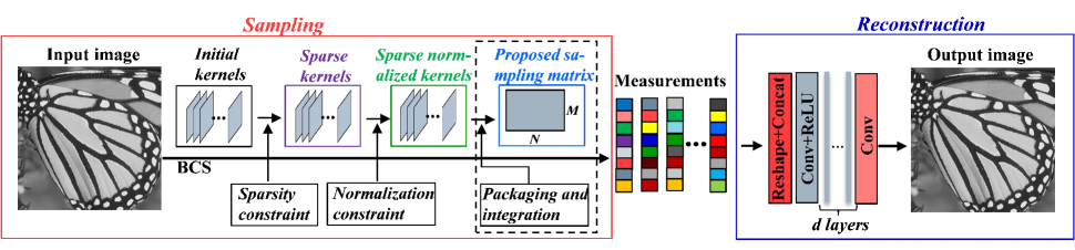
In traditional block-based compressed sensing (BCS) [9], each row of the sampling matrix $\bm{\Phi}$ can be considered as a filter. Therefore, the sampling process can be mimicked using a convolutional layer [10, 11]. Specifically, given an image $I$ with size $w\times h$, the measurement vectors of $I$ can be obtained by applying a convolutional operator to the image $\mathcal{Y}=\mathcal{C}_{B}(I)$ where $\mathcal{Y}$ is the set of measurement vectors and $\mathcal{C}_{B}(\cdot)$ denotes the convolution operation with kernel size $B\times B$ and stride size $B\times B$. The block size is $N_{B}=B\times B$ and the dimension of the measurements for each block is $N_{b}=\lfloor\frac{M}{N}N_{B}\rfloor$. However, these DNN-based methods pay more attention to the reconstruction accuracy, while ignoring some essential properties and several major drawbacks for the measurement matrix. In this paper, a sparse normalized measurement matrix is produced by using a novel convolutional layer with a sparsity constraint and a normalization constraint, which not only can be used in most of algorithms directly without any extra modification but also reduces the memory requirement and computing cost significantly.

Refer to caption Original$\backslash$PSNR$\backslash$SSIM Refer to caption GRM$\backslash$30.35$\backslash$0.9128 Refer to caption DSMM(0.01)$\backslash$32.61$\backslash$0.9604 Refer to caption DSMM(0.05)$\backslash$33.20$\backslash$0.9654 Refer to caption DSMM(0.1)$\backslash$33.23$\backslash$0.9656 Refer to caption DSMM(0.5)$\backslash$33.59$\backslash$0.9702 Refer to caption DSMM(0.9)$\backslash$33.61$\backslash$0.9707

Fig. 3: Visual quality comparison of Method MH [4] in the case of sampling ratio = 0.1 for image Baby in Set5

2.1.1 Sparsity Constraint
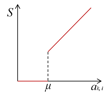
For $\bm{\Phi}$, we assume that the $k$th line of $\bm{\Phi}$ is denoted by $\Phi(k)=\{a_{k,1},a_{k,2},\cdot\cdot\cdot,a_{k,N_{B}}\}$ and the sparsity degree by $\mathcal{SD}(\bm{\Phi})=\frac{\mathcal{NUM}(\bm{\Phi},!0)}{N_{b}N_{B}}$, where $\mathcal{NUM}(\bm{\Phi},!0)$ indicates the numbers of nonzero elements in $\bm{\Phi}$ and $N_{b}N_{B}$ is the total elements in $\bm{\Phi}$. In order to produce the target sampling matrix with predefined sparsity degree $\mathcal{SD}(\bm{\Phi})=\alpha$ $(0\leqslant\alpha<1)$, a sparsity constraint is defined as follows:

$\displaystyle\mathcal{S}(a_{k,i})=\begin{cases}0&\text{$|a_{k,i}|$ $\leqslant$ $\mu$}\\ a_{k,i}&\text{$|a_{k,i}|$ $>$ $\mu$}\end{cases}$ (3)

where $k=1,2,\cdot\cdot\cdot,N_{b}$, $i=1,2,\cdot\cdot\cdot,N_{B}$ and $\mu$ is the $(1-\alpha)N_{b}N_{B}$-$th$ smallest element in $|\bm{\Phi}|$. Fig. 2 shows the details of the sparsity constraint and its approximate derivative. Through this constraint, expected $\bm{\Phi}$ with different sparsity degree can be generated, which reduces the storage cost and computational complexity greatly.

2.1.2 Normalization Constraint

In most of CS literatures [3, 4, 5, 6], the measurement matrix is normalized to control the range of measurements. Mathematically, the normalization constraint of $\bm{\Phi}$ is defined by:

$\displaystyle\sum_{i=1}^{N_{B}}a_{k,i}^{2}=1,\ \ k=1,2,\cdot\cdot\cdot,N_{b}$ (4)

In fact, $\Phi(k)$ is the $k$th kernel of convolutional layer in the sampling sub-network and $a_{k,i}$ is the $i$th value of this kernel. In this paper, in order to generate normalized sampling matrix, we applied a normalization constraint to the parameters of the convolutional layer in the sampling sub-network. The normalization constraint for $k$th kernel can be formulated as:

$\displaystyle\mathcal{F}(s_{k,j})=\frac{s_{k,j}}{\sqrt{\sum_{i=1}^{N_{B}}s_{k,i}^{2}}},\ \ j=1,2,\cdot\cdot\cdot,N_{B}$ (5)

where $s_{k,j}=\mathcal{S}(a_{k,j})$ and its derivative executed as:

$\displaystyle\mathcal{F}^{{}^{\prime}}(s_{k,j})=\frac{\sqrt{\omega}-\frac{s_{k,j}^{2}}{\sqrt{\omega}}}{\sqrt{\omega}},\ \ \ \omega=\sum_{i=1}^{N_{B}}s_{k,i}^{2}$ (6)

Through Eq. 5, we got the normalized parameters, namely the normalized sampling matrix. Then this sampling matrix will be used to sample the original images.

Table 1: Quantitative evaluation of GRM and DSMM for method GSR: Average PSNR$\backslash$SSIM at different sampling ratios 0.1, 0.2 and 0.3 on datasets Set5. Red text indicates the best performance
Alg. GSR [6]
sampling ratio 0.1 0.2 0.3
GRM 30.6$\backslash$0.88 34.4$\backslash$0.92 37.1$\backslash$0.95
DSMM-1% 32.0$\backslash$0.88 34.9$\backslash$0.93 37.1$\backslash$0.95
DSMM-2% 32.6$\backslash$0.89 35.5$\backslash$0.93 37.8$\backslash$0.96
DSMM-5% 32.7$\backslash$0.90 35.6$\backslash$0.94 38.1$\backslash$0.96
DSMM-20% $\textbf{\color[rgb]{1,0,0}33.0}\backslash\textbf{\color[rgb]{1,0,0}0.91}$ $\textbf{\color[rgb]{1,0,0}36.1}\backslash\textbf{\color[rgb]{1,0,0}0.95}$ $\textbf{\color[rgb]{1,0,0}38.5}\backslash\textbf{\color[rgb]{1,0,0}0.97}$
DSMM-50% 32.9$\backslash\textbf{\color[rgb]{1,0,0}0.91}$ $\textbf{\color[rgb]{1,0,0}36.1}\backslash\textbf{\color[rgb]{1,0,0}0.95}$ 38.4$\backslash\textbf{\color[rgb]{1,0,0}0.97}$
DSMM-90% 32.9$\backslash\textbf{\color[rgb]{1,0,0}0.91}$ 36.0$\backslash\textbf{\color[rgb]{1,0,0}0.95}$ 38.4$\backslash\textbf{\color[rgb]{1,0,0}0.97}$
DSMM 32.9$\backslash\textbf{\color[rgb]{1,0,0}0.91}$ 36.0$\backslash\textbf{\color[rgb]{1,0,0}0.95}$ 38.4$\backslash\textbf{\color[rgb]{1,0,0}0.97}$
Gain $\textbf{+2.4}\backslash\textbf{0.03}$ $\textbf{+1.7}\backslash\textbf{0.03}$ $\textbf{+1.4}\backslash\textbf{0.02}$
Table 2: Quantitative evaluation of GRM and DSMM for method MH and CoS: Average PSNR$\backslash$SSIM at different sampling ratios 0.1, 0.2 and 0.3 on datasets Set5. Red text indicates the best performance
Alg. MH [4] CoS [5] Avg.
sampling ratio 0.1 0.2 0.3 0.1 0.2 0.3
GRM 27.4$\backslash$0.803 30.7$\backslash$0.881 32.6$\backslash$0.911 28.3$\backslash$0.819 30.0$\backslash$0.858 30.6$\backslash$0.871 29.9$\backslash$0.857
DSMM-1% 29.0$\backslash$0.853 31.9$\backslash$0.905 32.3$\backslash$0.911 30.1$\backslash$0.864 32.2$\backslash$0.898 33.5$\backslash$0.910 31.5$\backslash$0.890
DSMM-2% 29.3$\backslash$0.861 32.3$\backslash$0.913 32.5$\backslash$0.919 30.4$\backslash$0.872 32.7$\backslash$0.905 33.8$\backslash$0.920 31.8$\backslash$0.898
DSMM-5% 29.7$\backslash$0.868 32.7$\backslash$0.921 32.9$\backslash$0.922 30.7$\backslash$0.878 33.0$\backslash$0.914 34.4$\backslash$0.927 32.2$\backslash$0.905
DSMM-20% 30.0$\backslash$0.873 33.0$\backslash$0.925 33.2$\backslash$0.930 31.0$\backslash$0.884 33.4$\backslash$0.918 34.6$\backslash$0.930 32.5$\backslash$0.910
DSMM-50% $\textbf{\color[rgb]{1,0,0}30.1}\backslash$0.880 $\textbf{\color[rgb]{1,0,0}33.3}\backslash\textbf{\color[rgb]{1,0,0}0.934}$ $\textbf{\color[rgb]{1,0,0}33.5}\backslash\textbf{\color[rgb]{1,0,0}0.932}$ $\textbf{\color[rgb]{1,0,0}31.1}\backslash\textbf{\color[rgb]{1,0,0}0.888}$ $\textbf{\color[rgb]{1,0,0}33.7}\backslash\textbf{\color[rgb]{1,0,0}0.926}$ $\textbf{\color[rgb]{1,0,0}34.8}\backslash\textbf{\color[rgb]{1,0,0}0.932}$ $\textbf{\color[rgb]{1,0,0}32.8}\backslash\textbf{\color[rgb]{1,0,0}0.915}$
DSMM-90% $\textbf{\color[rgb]{1,0,0}30.1}\backslash\textbf{\color[rgb]{1,0,0}0.881}$ $\textbf{\color[rgb]{1,0,0}33.3}\backslash\textbf{\color[rgb]{1,0,0}0.934}$ 33.3$\backslash$0.930 31.0$\backslash$0.886 33.5$\backslash$0.923 34.6$\backslash$0.930 32.6$\backslash$0.914
DSMM $\textbf{\color[rgb]{1,0,0}30.1}\backslash\textbf{\color[rgb]{1,0,0}0.881}$ 33.1$\backslash\textbf{\color[rgb]{1,0,0}0.934}$ 33.3$\backslash$0.931 30.9$\backslash$0.884 33.4$\backslash$0.921 34.7$\backslash$0.931 32.6$\backslash$0.914
Gain $\textbf{+2.7}\backslash\textbf{0.078}$ $\textbf{+2.6}\backslash\textbf{0.054}$ $\textbf{+0.9}\backslash\textbf{0.021}$ $\textbf{+2.8}\backslash\textbf{0.069}$ $\textbf{+3.7}\backslash\textbf{0.068}$ $\textbf{+4.2}\backslash\textbf{0.061}$ $\textbf{+2.9}\backslash\textbf{0.058}$

2.2 Reconstruction Sub-network

The measurements is hardly to be used to evaluate the image reconstruction quality directly. In order to improve the CS reconstruction performance, the image reconstruction sub-network are utilized to help enhance the sampling sub-network. For the reconstruction algorithms of CS, many optimization-based [3, 4, 5, 6] and deep learning based methods [12, 13, 11] have been proposed. Considering the hardness of calculating derivatives for the optimization-based methods and inspired by the aforementioned deep learning based works, we utilize a “reshape+concat” layer and several convolutional layers to reconstruct original images as shown in Fig. 1. Given the compressed measurement vector, we utilize a “reshape+concat” layer [11] to obtain a feature map with the same size as the original block. Then the further nonlinear reconstruction is executed by using several convolutional layers, which has the same configuration with CSNet [11] (d=3). In our network, this reconstruction sub-network has two important missions. One is that reconstructing the target images from its measurements. Another is providing guidance for the optimization of sampling sub-network.

3 Training Details and Experiments

In our model, the sampling sub-network and the reconstruction sub-network are optimized jointly. In this section, we describe the training details as well as the experimental results. Given the input image block $x$, our goal is to obtain highly compressed measurement $y$ with the sampling sub-network, and then accurately recover it to the original input image block $x$ with the reconstruction sub-network. The input and the label are all image block $x$ itself for training. Therefore, the training dataset can be represented as $\{x_{i},x_{i}\}_{i}^{N}$. The mean square error (MSE) is adopted as the cost function of our network. The optimization objective is represented as

$\displaystyle\min\frac{1}{2N}\sum_{i=1}^{N}\|g(x_{i};\theta_{s},\theta_{r})-x_{i}\|_{2}^{2}$ (7)

where $g$ is the operations of our network. $\theta_{s}$ and $\theta_{r}$ is the parameters of sampling sub-network and reconstruction sub-network. $g(x_{i};\theta_{s},\theta_{r})$ is the final CS reconstructed output with respect to $x_{i}$.

Algorithm 1 The training process of the proposed network for one iteration
Initiate the parameters $\theta_{s}$, $\theta_{r}$ of network
$\{x_{i}$, $x_{i}\}$
$\theta_{G}\leftarrow global\ variable$
function Forward($x_{i}$)
     $\theta_{G}\leftarrow\theta_{s}$
     $\theta_{s}\leftarrow sparsity\ constraint$
     for $kernel$ in $\theta_{s}$ do
         $kernel\leftarrow normalization\ constraint$
     end for
     return $Output\leftarrow\|g(x_{i},\ \theta_{s},\ \theta_{r})-x_{i}\|_{2}^{2}$
end function
function Backward($Output,\ x_{i}$)
     $\frac{d(Output)}{d(\theta_{s})},\ \frac{d(Output)}{d(\theta_{r})}\leftarrow\nabla(x_{i},\ Output)$
     $\theta_{r}\leftarrow\theta_{r}-\gamma\frac{d(Output)}{d(\theta_{r})}\ \ \ (\gamma\ is\ learning\ rate)$
     $\theta_{s}\leftarrow\theta_{G}$
     $\theta_{s}\leftarrow\theta_{s}-\gamma(\frac{d(Output)}{d(\theta_{s})}*\mathcal{F}^{{}^{\prime}}(\mathcal{S}(\theta_{s})))$
end function
$\nabla\ is\ the\ gradient\ back\ propagation.$

We use the training set of the BSDS500 database [14] for training, and the its validation set for validation. We set the patch size as 96$\times$96, batch size as $32$ and block size as 32 ($B$=32). We augment the training data in two ways: $(i)$ Randomly scale between $[0.8,1.2]$. $(ii)$ Flip the images horizontally with a probability of 0.5. The DSMM is trained with the Matlab toolbox MatConvNet [15] on a Titan X GPU. The momentum parameter is set as 0.9 and weight decay as $1e$-$4$. We train our model for 100 epochs and each epoch iterates 600 times. Standard gradient descent (SGD) is used to optimize all network parameters. For the learning rate, the first 30 epochs is set $1e$-$3$. The following 40 epochs are declined equably from $1e$-$4$ to $1e$-$6$ and the last 30 epochs is set as $1e$-$6$. Algorithm 1 shows the details of training process of our framework for one iteration.

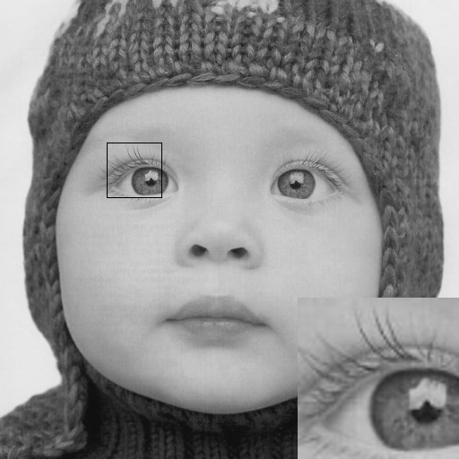
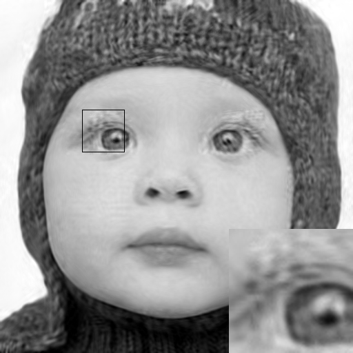
We evaluate the performance of the proposed DSMM for CS reconstruction in the algorithms MH [4], CoS [5] and GSR [6]. Specifically, we replace the gaussian random matrix with our DSMM and recover the original images with these methods. To evaluate the performance of each algorithm, we investigate three different sampling ratios 0.1, 0.2, 0.3 and seven different sparse degrees 0.01(DSMM-1%), 0.02(DSMM-2%), 0.05(DSMM-5%), 0.2(DSMM-20%), 0.5(DSMM-50%), 0.9(DSMM-90%), 1.0 (DSMM) with assessment criteria PSNR and SSIM. The comparisons with various algorithms on benchmark Set5 are provided in Table 1 and Table 2. Some visual comparisons shown in Figs. 3. demonstrate that our proposed DSMM preserves much sharper edges and finer details. In regular CS applications, DSMM-20% has almost achieved the best performances.

4 Conclusion

In this paper, a novel deep neural network based sparse measurement matrix (DSMM) for CS sampling of natural images is proposed by utilizing a deep convolutional network, which not only ensure sufficient information in the measurements for CS reconstruction but also reduces the memory requirement and computing cost significantly. Experimental results show that the proposed DSMM greatly enhances the existing performance of CS reconstruction when compared with GRM.

5 Acknowledgements

This work is partially funded by the Major State Basic Research Development Program of China (973 Program 2015CB351804) and the National Natural Science Foundation of China under Grant No. 61572155 and 61672188.

References

  • [1] E. J. Candès, J. Romberg, and T. Tao, “Robust uncertainty principles: Exact signal reconstruction from highly incomplete frequency information,” IEEE Transactions on Information Theory, vol. 52, no. 2, pp. 489–509, 2006.
  • [2] D. L. Donoho, “Compressed sensing,” IEEE Transactions on Information Theory, vol. 52, no. 4, pp. 1289–1306, 2006.
  • [3] C. Li, W. Yin, H. Jiang, and Y. Zhang, “An efficient augmented lagrangian method with applications to total variation minimization,” Computational Optimization and Applications, vol. 56, no. 3, pp. 507–530, 2013.
  • [4] C. Chen, E. W. Tramel, and J. E. Fowler, “Compressed-sensing recovery of images and video using multihypothesis predictions,” IEEE Conference Record of the Forty Fifth Asilomar Conference on Signals, Systems and Computers (ASILOMAR), pp. 1193–1198, 2011.
  • [5] J. Zhang, D. Zhao, C. Zhao, R. Xiong, S. Ma, and W. Gao, “Compressed sensing recovery via collaborative sparsity,” IEEE Data Compression Conference (DCC), pp. 287–296, 2012.
  • [6] J. Zhang, D. Zhao, and W. Gao, “Group-based sparse representation for image restoration,” IEEE Transactions on Image Processing, vol. 23, no. 8, pp. 3336–3351, 2014.
  • [7] K. Q. Dinh, H. J. Shim, and B. Jeon, “Measurement coding for compressive imaging using a structural measuremnet matrix,” IEEE International Conference on Image Processing (ICIP), pp. 10–13, 2013.
  • [8] X. Gao, J. Zhang, W. Che, X. Fan, and D. Zhao, “Block-based compressive sensing coding of natural images by local structural measurement matrix,” IEEE Data Compression Conference (DCC), pp. 133–142, 2015.
  • [9] L. Gan, “Block compressed sensing of natural images,” IEEE International Conference on Digital Signal Processing, pp. 403–406, 2007.
  • [10] A. Adler, D. Boublil, M. Elad, and M. Zibulevsky, “A deep learning approach to block-based compressed sensing of images,” arXiv preprint arXiv:1606.01519, 2016.
  • [11] W. Shi, F. Jiang, S. Zhang, and D. Zhao, “Deep networks for compressed image sensing,” IEEE International Conference on Multimedia and Expo (ICME), pp. 877–882, 2017.
  • [12] A. Mousavi, A. B. Patel, and R. G. Baraniuk, “A deep learning approach to structured signal recovery,” IEEE Allerton Conference on Communication, Control, and Computing (Allerton), pp. 1336–1343, 2015.
  • [13] K. Kulkarni, S. Lohit, P. Turaga, R. Kerviche, and A. Ashok, “Reconnet: Non-iterative reconstruction of images from compressively sensed random measurements,” IEEE Conference on Computer Vision and Pattern Recongnition (CVPR), pp. 449–458, 2016.
  • [14] P. Arbelaez, M. Maire, C. Fowlkes, and J. Malik, “Contour detection and hierarchical image segmentation,” IEEE Transactions on Pattern Analysis and Machine Intelligence, vol. 33, no. 5, pp. 898–916, 2011.
  • [15] A. Vedaldi and K. Lenc, “Matconvnet: Convolutional neural networks for matlab,” ACM International Conference on Multimedia, pp. 689–692, 2015.
Conversion to HTML had a Fatal error and exited abruptly. This document may be truncated or damaged.