Evaluating Ex Ante Counterfactual Predictions Using Ex Post Causal Inference

Abstract

We derive a formal, decision-based method for comparing the performance of counterfactual treatment regime predictions using the results from randomized experiments. Our approach allows us to quantify and assess the statistical significance of differential performance for optimal treatment regimes estimated from structural models, extrapolated treatment effects, expert opinion, and other methods. We apply our method to evaluate optimal treatment regimes for conditional cash transfer programs across countries where predictions are generated using data from experimental evaluations in other countries and pre-program data in the country of interest.

1 Introduction

Social scientists often provide recommendations about the implementation of policies, which determine whether and in what manner a given treatment should be applied in some target context. Crucial to this task is generating counterfactual predictions to inform such recommendations. The methods to which social scientists turn for this purpose are varied. They include quantitative extrapolations from existing randomized evaluations or observational studies, predictions based on structural models that interpret behavioral patterns in the target context, and more subjective expert opinions, among others.

Our goal in this paper is to offer a formal framework for evaluating the relative success of methods for generating policy recommendations. We evaluate the success of ex ante policy recommendations that can draw on pre-existing experiments and descriptive data to recommend a treatment assignment in a target context. Then, we conduct an ex post evaluation of the recommendation, based on information from experiments in the target context. We are thus able to quantify and assess the statistical significance, ex post, of the differential performance of various methods for generating ex ante recommendations. These ex post assessments can inform choices over methods to produce ex ante recommendations for new contexts where experimental data are not yet available.

Our framework is decision-based, considering optimal choices for a social planner seeking to maximize a welfare objective subject. We consider a linear social welfare function, although the framework could take into consideration preferences over inequality, uncertainty, status quo bias, or other modifications. The planner is thought to face constraints that limit the set of policy options. Multiple methods may yield identical results for basic types of recommendations — e.g., they may agree on whether the treatment is harmful or helpful on average, in which case they would make the same recommendation regarding the alternatives of “treat everyone” versus “treat no one.”

But when it comes to estimating optimal policies, methods may differ in their recommendations. Such differences in recommendations would be due to different methods’ predictions about how different types of people respond to treatment (Manski, 2004; Dehejia, 2005; Hirano and Porter, 2009; Imai and Strauss, 2011; Kitagawa and Tetenov, 2017; Athey and Wager, 2017) . The wider the range of admissible policy options, the wider is the scope for methods to differ in their recommendations and thus in their relative performance. Another way to put this is that the more refined the policy decision at stake, the more we need to ask of the methods, and thus the more refined will be our judgment about the performance of different methods.

What we refer to as a “method” is an approach for determining which of these policy options should be implemented. These include reduced form methods that rely on conditional unconfoundedness to extrapolate conditional treatment effects using existing experimental or observational evaluations from other contexts, as in Hotz et al. (2005) and Dehejia et al. (2017). Another class of methods includes meta-analytical methods that model heterogeneity across contexts, as in Dehejia (2003), Meager (2016), and Vivalt (2016). A third class of methods includes structural models. These include models that interpret behavioral patterns among untreated observations within the target context so as to generate counterfactual predictions about outcomes under treatment, as in Todd and Wolpin (2006) and Todd and Wolpin (2008). They also include approaches that estimate of some structural model parameters using untreated units in the target context and others from available experimental evidence, as in Attanasio et al. (2012). Hybrids of reduced form and structural methods are also available, as in Gechter (2016). Finally, a fifth class of methods includes the solicitation of subjective opinions of experts, as discussed in Banerjee et al. (2016) and applied in DellaVigna and Pope (2017).

In our application, we allow methods to draw on existing experimental data from other contexts as well as data on covariates and untreated outcomes in the target context. The resulting recommendations are thus “ex ante” insofar as they are made under uncertainty about the distribution of potential outcomes under treatment. An assessment is then done ex post, using data from experiments that reveal the distribution of potential outcomes under treatment. Our analysis allows us to determine, ex post, whether the policy recommendation from one or another method performed significantly better in terms of promoting welfare.

We use our framework to evaluate conditional cash transfer policies for increasing children’s school enrollment, a policy subject to widespread consideration around the world (Parker and Vogl, 2018). We begin with an illustrative example of making a policy recommendation for a conditional cash transfer program in Morocco. Ex ante, the methods can draw upon data from a conditional cash transfer experiment in Mexico—specifically, the PROGRESA randomized evaluation—as well as covariates and untreated outcome data in Morocco. We consider four methods: (1) simple reduced form extrapolation of conditional treatment effects by age-sex strata from Mexico to Morocco, (2) more sophisticated conditional average treatment effect extrapolation using Athey et al. (2019)’s Generalized Random Forest (GRF) algorithm, (3) a static, semi-parametric structural (SPS) model based on Todd and Wolpin (2008), (4) a dynamic, parametric structural model based on Attanasio et al. (2012) (AMS). We then assess, ex post, the performance of the two methods using the results of the randomized evaluation conducted by Benhassine et al. (2015).

The results show that methods (1) and (4) perform best in this particular case despite making fairly different policy recommendations. The GRF appears to suffer from “contextual overfitting” in the sense that the extra heterogeneity it detects is more idiosyncratic to PROGRESA than the basic heterogeneity captured by a simple stratification exercise. SPS’s non-parametric component is perhaps too flexible, leading to a more standard overfitting problem despite some regularization. These results are preliminary, based on one reference-target pair out of 7 different CCT contexts we have harmonized data from. Our full set of findings are intended to speak to the question of whether policy recommendations should rely on internally valid evidence generated outside the target context, or whether one should rely on potentially confounded evidence from within the target context, as in Pritchett and Sandefur (2013).

Our methodological contribution is a formal framework for evaluating policy recommendations based on counterfactual predictions from competing methods. Our aim is to provide tools that are more general in speaking to policy recommendations than the relatively informal and case-specific model validation exercises that regularly appear in the applied microeconomics literature; see, for example, Todd and Wolpin (2006), Keane and Wolpin (2007), Duflo et al. (2012), and Wolpin (2013), who each use predictions into holdout samples to evaluate the fit of structural models. Our framework for evaluating policy recommendation methods builds on Pesaran and Skouras (2002) and Granger and Machina (2006)’s notion of using information on the intended use of predictions as a basis for judging methods, foundational work on forecast evaluation theory by Diebold and Mariano (1995), White (2000), and Hansen et al. (2011), as well as work on prediction-based model comparisons by Keane and Wolpin (2007), Wolpin (2007), Wolpin (2013), Schorfheide and Wolpin (2012), and Schorfheide and Wolpin (2016). We see our work as complementary to research by DellaVigna and Pope (2017) on evaluating the quality of experts’ ex ante forecasts by using experimental data ex post. Manski (1996, 2004), Dehejia (2005), Hirano and Porter (2009), Tetenov (2012), Kitagawa and Tetenov (2017), and Athey and Wager (2017) address the issue of deriving optimal treatment regimes in decision-theoretic terms in sample; we extend these ideas to the evaluation of methods out of sample as well.

Evaluating methods through the lens of a decision problem is in line with Arrow (1972), and presents an attractive alternative to model comparison based on Kullback-Leibler divergence (as in Vuong, 1989). Selection based on Kullback-Leibler superiority may be inadequate for a particular decision problem (Marschak and Miyasawa, 1968) . Finally, our application to the conditional cash transfer programs draws on the synthesis discussions in Banerjee et al. (2017) and Garcia and Saavedra (2017) as well as the specific data and analyses conducted by De Janvry and Sadoulet (2006), Todd and Wolpin (2006), and Attanasio et al. (2012) for Mexico and Benhassine et al. (2015) for Morocco.

2 Setting

Let $\mathcal{M}$ define a set of methods under consideration. A method $m\in\mathcal{M}$ produces predictions for a set of real-valued treatment conditions, $\mathcal{T}$, finite. Suppose that the status quo treatment condition is given by $t=0\in\mathcal{T}$ for all $m\in\mathcal{M}$. Considering our application below, we can imagine that $m$ could be a reduced form extrapolation method for predicting responses to different subsidy schedules, which are elements in the set $\mathcal{T}$, including the no subsidy condition, $t=0$.

We consider a social planner interested in using data from a set of reference contexts to devise welfare-maximizing policies in a set of target contexts. Suppose contexts are indexed by $c\in\{1,...,C\}$. Let $D_{c}$ be an indicator variable dividing the contexts into target and reference contexts, such that $D_{c}=1$ when $c$ is a target context and $D_{c}=0$ when $c$ is a reference context. The planner wants to assess the methods in $\mathcal{M}$ according to their ability to assign individuals to treatments from within $\mathcal{T}$ in a way that maximizes the planner’s social welfare function in the target contexts, subject to potential constraints on feasible treatments.

A set of treatment conditions, $\mathcal{T}_{c}\subseteq\mathcal{T}$, is active in each context $c$, although methods may be able to use data from a set $\mathcal{T}_{c}$ to generate counterfactual predictions for treatments that are outside this set. For example, structural methods can generate counterfactual predictions for treatment effects with treatments that have never been implemented. For the target contexts, we suppose that ex ante, $\mathcal{T}_{c}=\{0\}$, meaning only data on the status quo conditions are available. In the reference contexts, ex ante, $\mathcal{T}_{c}$ may contain treatments other than just the status quo. Thus, in the target contexts, only the $t=0$ treatment is active prior to the implementation of policy, and the social planner is seeking a recommendation on how to introduce treatments from a feasible set of options so as to maximize welfare. The recommendations are based on methods that make counterfactual predictions for the target contexts. We observe an $J$-vector of context level characteristics, $V_{c}$, which contains the indicator, $D_{c}$, as well as $J-1$ other attributes, such that ${\rm Supp}\,(V_{c})=\mathcal{V}\subseteq\mathbb{R}^{J}$.

Within a given context $c$, let $i$ index individuals. Each context is governed by a probability distribution, $\mathbb{P}_{c}$, on the following: an individual-level treatment variable, $T_{ic}$, where ${\rm Supp}\,{(T_{ic})}=\mathcal{T}_{c}$; a $K$-vector of individual-level covariates, $W_{ic}$, with ${\rm Supp}\,{(W_{ic})}=\mathcal{W}_{c}\subseteq\mathbb{R}^{K}$; and an individual-level potential outcome function, $Y_{tic}:\mathcal{T}_{c}\rightarrow\mathbb{R}$, that maps treatments to outcomes. These outcomes measure individual wellbeing from the planner’s perspective. We suppose the following conditions on the outcome data:

C0.

$|\mathbb{E}\,_{c}[Y_{tic}]|<\infty$ and $0<\mathbb{V}\,_{c}[Y_{tic}]<\infty$ for all $t\in\mathcal{T}_{c}$ and $c\in\{1,...,C\}$.

Let $Y_{it}=Y_{T_{ic}ic}$ be the observed outcome for unit $i$ in context $c$. The observed data consist of the context level characteristics and individual-level data, $O_{ic}=(V_{c},W_{ic},T_{ic},Y_{ic})$, for random samples of individuals $i\in\{1,...,n_{c}\}$ across contexts $c=\{1,...,C\}$.

For simplicity, we focus on the case where we can take individual-level treatments to be binary, in which case $\mathcal{T}=\{0,1\}$, where $t=0$ is a status quo control condition and $t=1$ a treated condition. Then, individuals’ potential outcomes are $\left(Y_{1ic},Y_{0ic}\right)$ and observed outcomes are given by $Y_{ic}=T_{ic}Y_{1ic},+(1-T_{ic})Y_{0ic}$. For a context $c\in\{1,..,C\}$, consider the following conditions on the data generating process defining $\mathbb{P}_{c}$:

C1.

conditional random assignment, $\left(Y_{1ic},Y_{0ic}\right)\mathchoice{\mathrel{\hbox to0.0pt{$\displaystyle\perp$\hss}\mkern 2.0mu{\displaystyle\perp}}}{\mathrel{\hbox to0.0pt{$\textstyle\perp$\hss}\mkern 2.0mu{\textstyle\perp}}}{\mathrel{\hbox to0.0pt{$\scriptstyle\perp$\hss}\mkern 2.0mu{\scriptstyle\perp}}}{\mathrel{\hbox to0.0pt{$\scriptscriptstyle\perp$\hss}\mkern 2.0mu{\scriptscriptstyle\perp}}}T_{ic}|W_{ic}=w$ for all $w\in\mathcal{W}_{c}$;

C2.

overlap, where probabilities of assignment, $p_{c}(w):=\Pr[T_{ic}=1|W_{ic}=w]$, are interior such that $0<b_{0}<p_{c}(w)<b_{1}<1$ for all $w\in\mathcal{W}_{c}$, and

C3.

stable unit treatment value assumption (SUTVA; Rubin, 1980), such that for $T_{ic}=t$, $Y_{ic}=Y_{tic}$ with probability 1.

When conditions C1-C3 hold, the conditional (on covariates) potential outcome distributions for both the treatment and control groups in the reference contexts are identified.

In our setting, we suppose that, ex ante, we are working with a random sample for which conditions C1-C3 hold in the reference contexts (for which $D_{ic}=0$). However, in the the target contexts (for which $D_{c}=1$), we suppose that, ex ante, we have a random sample only for units with $T_{ic}=0$, while the covariate distributions are also identified. As such, ex ante, the distributions $\mathbb{P}_{c}[(Y_{0ic},W_{ic})|V_{c},D_{c}=0]$, $\mathbb{P}_{c}[(Y_{1ic},W_{ic})|V_{c},D_{c}=0]$, and $\mathbb{P}_{c}[(Y_{0ic}(0),W_{ic})|V_{c},D_{c}=1]$ are identified. The methods make use of these distributions to derive policy recommendations. Once the recommendations are submitted, we then suppose that the conditions C1-C3 obtain in the target contexts, in which case the $\mathbb{P}_{c}[(Y_{1ic},W_{ic})|V_{c},D_{c}=1]$ distributions are revealed. This allows the planner to judge, ex post, the quality of the methods in terms of how their recommendations fair with respect to welfare.

Conditions C1-C3 include situations where we have a set of randomized experiments that we can feed into a set of methods to produce ex ante recommendations for a new target context. These conditions also admit observational studies in which conditional independence and overlap of treatment assignment holds over the covariate space, $\mathcal{W}_{c}$, although for the time being we focus on randomized experiments. Our specification of the potential outcomes, combined with assumption C3, rules out “interference” (Cox, 1958, p. 19), including general equilibrium effects. We consider this a starting point for our analysis. Generalizations could consider situations where interference is present, and derive criteria for judging methods by working with causal quantities that are identified under interference (Hudgens and Halloran, 2008; Aronow and Samii, 2017).

3 Planner’s Objective and Ex Ante Recommendations

We can define the planner’s objective in context $c$ in general terms as

$$\max_{\pi}\mathcal{U}(\mathbb{P}_{c}(\pi))$$

where $\pi:\mathcal{V}\times\mathcal{W}_{c}\rightarrow\{0,1\}$ is a treatment assignment rule that takes context $c$’s contextual attributes and an individual’s covariate values and maps them to a treatment assignment. Then, $\mathbb{P}_{c}(\pi)$ is the joint potential outcome-covariate distribution induced by $\pi$. The restriction to $\{0,1\}$ for each individual in the target context follows from our focus on binary treatments. If a richer set of treatment values $\mathcal{T}$ were under consideration, the rule $\pi$ could assign distribution functions over this $\mathcal{T}$ on the basis of covariate values. Sometimes the set of conditional treatment assignments that maximizes this objective ex ante is non-unique—i.e., there are ties. For example, multiple units may share the same covariate value. The treatment assignment that maximizes the objective may assign some fraction of such units to treatment. Then, all permutations of assignments would yield the same ex ante value for the objective. We assume that $\pi$ encodes a tie-breaker rule that is unconditionally statistically independent and equalizes probability of treatment for such tied units.

Current approaches to this problem (as in Manski, 2004 and Tetenov, 2012) consider social welfare that is linear in expected treatment and control outcomes, what Hirano and Porter (2019) refer to as utilitarian welfare. We adopt the same approach. We also incorporate treatment opportunity costs by adding a cost-effectiveness term to the planner’s objective. This increases the planner’s sensitivity to over- and under-estimation of the treatment effects in generating treatment rules. We suppose that we are operating in context $c$, and therefore suppress the associated indexing except when necessary for clarification. Thus, we define

$$\mathcal{U}(\mathbb{P}(\pi))=$$

$$\mathbb{E}\,\left\{\pi(W_{i})\mathbb{E}\,\left[Y_{1i}-Y_{0i}-\frac{C(W_{i},Y_{1i})}{\kappa}\bigg{|}W_{i}\right]+(1-\pi(W_{i}))\mathbb{E}\,\left[\frac{C(W_{i},Y_{1i})}{\kappa}-(Y_{1i}-Y_{0i})\bigg{|}W_{i}\right]\right\}$$

$$=2\mathbb{E}\,\left\{\pi(W_{i})\mathbb{E}\,\left[Y_{1i}-Y_{0i}-\frac{C(W_{i},Y_{1i})}{\kappa}\bigg{|}W_{i}\right]\right\}-\mathbb{E}\,\left[Y_{1i}-Y_{0i}-\frac{C(W_{i},Y_{1i})}{\kappa}\right],$$

where $\kappa>0$ is the level of cost effectiveness at which the planner is indifferent between allocating funds to treat an individual and using the funds for some alternative purpose (Garber and Phelps, 1997; Dhaliwal et al., 2011), and $C(w,y)\geq 0$ is the marginal cost function for treating an individual with covariate value $w$ and treated outcome $y$. Choice of a treatment assignment with this specification will be equivalent to operating under a budget constraint that must be satisfied in expectation ex ante (cf. Bhattacharya and Dupas, 2012, versus ex post, as in Kitagawa and Tetenov, 2017), where the marginal value of relaxing the budget constraint is $1/\kappa$.

The prediction method $m$ translates the planner’s objective into an ex ante recommendation for a treatment assignment rule, $\pi_{m}$. Method $m$ does not have access to $\mathbb{P}$ and rather must rely on some approximation, $\widehat{\mathbb{P}}_{m}$. As such, method $m$ solves,

$$\pi_{m}=\text{arg}\max_{\pi}\mathcal{U}(\widehat{\mathbb{P}}_{m}(\pi)),$$

where $\widehat{\mathbb{P}}_{m}(\pi)$ can be informed by samples from the reference contexts and status quo data from the target. Under our specification of the welfare function, we have

$$\pi_{m}=\text{arg}\max_{\pi}\widehat{\mathbb{E}\,}_{m}\left\{\pi(W_{i})\widehat{\mathbb{E}\,}_{m}\left[Y_{1i}-Y_{0i}-\frac{C(w,Y_{1i})}{\kappa}\bigg{|}W_{i}\right]\right\}.$$

In practice, we will use a “plug-in” rule where $\hat{E}_{m}[\cdot]$ is generated from model $m$ estimated on the reference data and status quo data from the target (Hirano and Porter, 2019). The problem that method $m$ solves generates a decision rule analogous to Manski (2004)’s conditional empirical success rule:

$$\pi_{m}(w)=1\left\{\widehat{\mathbb{E}\,}_{m}\left[Y_{1i}-Y_{0i}-\frac{C(w,Y_{1i})}{\kappa}\bigg{|}w\right]\geq 0\right\}.$$

In our application to conditional cash transfer programs, the cost function takes a form that allows for further simplifications. Those details are presented below.

4 Ex Post Inference

The welfare contrast for two methods, $l$ and $m$, is given by

$$\Delta_{lm} =\mathbb{E}\,\left\{(\pi_{l}(W_{i})-\pi_{m}(W_{i}))\mathbb{E}\,\left[Y_{1i}-Y_{0i}-\frac{C(W_{i},Y_{1i})}{\kappa}\bigg{|}W_{i}\right]\right\},$$

where $2\Delta_{lm}$ would correspond to the difference in utilities as per our specification of $\mathcal{U}(\mathbb{P}(\pi))$ above. In constructing this ex post contrast, we condition on any data used to generate the $\hat{\mathbb{P}}$s. The welfare constrast $\Delta_{lm}$ is non-zero for values of $w$ for which the methods disagree on treatment assignment (i.e., $w$ for which $\pi_{l}(w)\neq\pi_{m}(w)$). It equals the marginalized value of the minimum-benefit-adjusted conditional average treatment effects when $m$ says to treat and $l$ says not to (or the reverse).

Ex post, we suppose that we obtain a random sample of experimental units in the target context for which conditions C1-C3 hold. We assume that in this ex post experiment, treatment assignment probabilities are given by $p(W_{i})$, and that these probabilities are known. The experimental data in our target context allow us to estimate this welfare contrast. Given a random sample of size $N$ in the target context, we consider an estimator for the linear welfare contrast based on inverse-probability of treatment weighting with normalized weights. This estimator is efficient among consistent estimators that avoid modeling of either the potential outcome surfaces or conditional treatment probabilities (Hirano et al., 2003; Lunceford and Davidian, 2004; Imbens and Wooldridge, 2009, 35). We define the estimator as

$$\hat{\Delta}_{lm}= \frac{\sum_{i=1}^{N}\frac{T_{i}}{p(W_{i})}\left(\pi_{l}(W_{i})-\pi_{m}(W_{i})\right)\left(Y_{i}-\frac{C(W_{i},Y_{i})}{\kappa}\right)}{\sum_{i=1}^{N}\frac{T_{i}}{p(W_{i})}}$$

$$-\frac{\sum_{i=1}^{N}\frac{(1-T_{i})}{1-p(W_{i})}\left(\pi_{l}(W_{i})-\pi_{m}(W_{i})\right)Y_{i}}{\sum_{i=1}^{N}\frac{(1-T_{i})}{1-p(W_{i})}}.$$

Inference for this estimator is based on the random sampling of $(Y_{i},T_{i},W_{i})$ values from $\mathbb{P}$ under conditions C0-C3:

Proposition 1.

Under conditions C0-C3, as $N\rightarrow\infty$

$$\frac{\sqrt{N}\left(\hat{\Delta}_{lm}-\Delta_{lm}\right)}{\sqrt{\hat{V}_{\Delta_{lm}}}}\overset{d}{\rightarrow}N(0,1),$$

where

$$\hat{V}_{\Delta^{g}_{lm}}= \frac{\sum_{i=1}^{N}\frac{T_{i}}{p(W_{i})^{2}}\left[(\pi_{l}(W_{i})-\pi_{m}(W_{i}))(Y_{i}-\frac{C(W_{i},Y_{i})}{\kappa})-\hat{\delta}_{1}\right]^{2}}{\sum_{i=1}^{N}\frac{T_{i}}{p(W_{i})}}$$

$$+\frac{\sum_{i=1}^{N}\frac{1-T_{i}}{[1-p(W_{i})]^{2}}\left[(\pi_{l}(W_{i})-\pi_{m}(W_{i}))Y_{i}-\hat{\delta}_{0}\right]^{2}}{\sum_{i=1}^{N}\frac{1-T_{i}}{1-p(W_{i})}},$$

and

$$\hat{\delta}_{1}=\frac{\sum_{i=1}^{N}\frac{T_{i}}{p(W_{i})}\left(\pi_{l}(W_{i})-\pi_{m}(W_{i})\right)(Y_{i}-\frac{C(W_{i},Y_{i})}{\kappa})}{\sum_{i=1}^{N}\frac{T_{i}}{p(W_{i})}}$$

$$\hat{\delta}_{0}=\frac{\sum_{i=1}^{N}\frac{1-T_{i}}{1-p(W_{i})}\left(\pi_{l}(W_{i})-\pi_{m}(W_{i})\right)Y_{i}}{\sum_{i=1}^{N}\frac{1-T_{i}}{1-p(W_{i})}}.$$

All proofs are contained in the appendix. Conditional on $W_{i}=w$, the recommendations, $\pi_{m}(w)$ and $\pi_{l}(w)$, are fixed. Our uncertainty about the welfare contrast is due to sampling and treatment assignment variation in the experimental data gathered in the target context that we use for the ex post assessment.

The ex post situation that we consider is simple in that all randomization and sampling occurs at the unit level and there is no causal interference in the outcome data generating process. Certainly the analysis could be extended to consider cluster randomization or cluster sampling, covariate adjustment, and targeting quantities that are identified under interference. For the present analysis, we stick with this relatively simple case.

Proposition 1 is sufficient to perform inference for any pair of methods. Hansen et al. (2011) provide a sequential multiple testing algorithm for establishing a “model confidence set” (MCS) of level $1-\alpha$, which allows one to distinguish a set of best performing algorithms with an asymptotic error rate of $\alpha$.

5 Empirical Application

For an empirical illustration, we use data from Mexico and Morocco on the effects of conditional cash transfers (CCTs) on primary school enrollment. We consider a policy scenario where a planner in Morocco is seeking recommendations for implementing a conditional cash transfer (CCT) program. The planner’s objective is defined as above, accounting for opportunity costs. We use data from randomized evaluations of the PROGRESA program in Mexico (Schultz, 2004; Behrman et al., 2005; De Janvry and Sadoulet, 2006; Todd and Wolpin, 2006; Attanasio et al., 2012) and the TAYSSIR program in Morocco (Benhassine et al., 2015). To construct the ex ante evaluations, we are limited to using the full data from Mexico and then the covariate and control group outcome data from Morocco. The ex post assessment is done using the full experimental data from Morocco.

5.1 General Setup

The outcome, $Y_{ic}$, is the school enrollment of child $i$. The covariate set, $\mathcal{W}_{c}$, is defined as the intersection pre-treatment characteristics on the PROGRESA and Moroccan questionnaires. The cost-effectiveness benchmark, $\kappa$, is based on gains from school enrollment. Montenegro and Patrinos (2014) report a 10% Mincer earnings premium for each additional year of schooling in Morocco. The average market earner in the Benhassine et al. (2015) sample gets $1578.20 per year. At a 5% discount rate, the net present value of an additional year spent in school is approximately $1,000. The treatment cost function, $C(W_{i},Y_{1i})$, is based on the value of the conditional transfer. In Morocco, for 6-7 year olds, this amounts to the following:

$$60\text{ MAD per month}\times 12\times\frac{0.1\text{ years of ed.}}{100USD}\times\frac{\text{1 USD}}{\text{8 MAD}}\times Y_{1i}=0.09Y_{1i}=\frac{C(w,Y_{1i})}{\kappa}.$$

Correspondingly, for 8-9 year olds the transfer value is 80 MAD per month, which means $0.12Y_{1i}=\frac{C(w,Y_{1i})}{\kappa}$, and for 10+ year olds, the transfer is 100 MAD per month, and so $0.15Y_{1i}=\frac{C(w,Y_{1i})}{\kappa}$. If we define these age specific multipliers as $g(Age_{i})$, then the objective for model $m$ reduces to,

$$\pi_{m} =\max_{\pi}\hat{\mathbb{E}\,}_{m}\left\{\pi(W_{i})\hat{\mathbb{E}\,}_{m}\left[(1-g(Age_{i}))Y_{1i}-Y_{0i}|W_{i}\right]\right\},$$

generating the decision rule

$$\pi_{m}(w)=1\left\{\hat{\mathbb{E}\,}_{m}\left[(1-g(Age_{i}))Y_{1i}-Y_{0i}\bigg{|}w\right]\geq 0\right\}.$$

This implies evaluating the signs of estimated conditional treatment effects on the adjusted outcome,

$$Y^{adj}_{ic}=T_{ic}(1-g(\text{Age}_{ic})Y_{ic}+(1-T_{ic})Y_{ic}.$$

We allow each method all observations and variables from PROGRESA ($D_{c}=0$), and observations from TAYSSIR with $D_{c}=1,T_{ic}=0,U_{ic}\leq 0.5$ where we assign $U_{ic}\sim U[0,1]$ independently from all other variables once (i.e., a random 50% split of the TAYSSIR control group). The methods use these data to compute $\pi_{m}(w)$ as defined above and then for methods $l$ and $m$, we compute $\widehat{\Delta}_{lm}$ as

$$\hat{\Delta}_{lm}= \frac{\sum_{\{i:D_{c}=1,T_{ic}=1\}}\frac{T_{i}}{p_{c}(W_{i})}\left(\pi_{l}(W_{i})-\pi_{m}(W_{i})\right)(1-g(Age_{i}))Y_{i}}{\sum_{\{i:D_{c}=1,T_{ic}=1\}}\frac{T_{i}}{p_{c}(W_{i})}}$$

$$-\frac{\sum_{\{i:D_{c}=1,T_{ic}=0,U_{ic}>0.5\}}\frac{(1-T_{i})}{1-p_{c}(W_{i})}\left(\pi_{l}(W_{i})-\pi_{m}(W_{i})\right)Y_{i}}{\sum_{\{i:D_{c}=1,T_{ic}=0,U_{ic}>0.5\}}\frac{(1-T_{i})}{1-p_{c}(W_{i})}},$$

where for the TAYSSIR experiment, $p_{c}(w)$ is known = $p_{c}$. The estimate for the variance is constructed analogously.

Methods

We consider methods that are already available from the current literature and that are straightforward to implement. We highlight assumptions on the joint distribution of random variables for each method. However, we are not concerned with testing these assumptions directly, as in Allcott (2015a), Dehejia et al. (2017). Instead, we list them as part of the specification of each method. We are interested in assessing the relative empirical performance of the methods, all of which we view as likely misspecified (Wolpin, 2007).

The first two methods rely on reduced-form extrapolation of conditional treatment effects, as per, e.g., Hotz et al. (2005) and Dehejia et al. (2016). The reduced form approaches we use include a “low-tech” version that simply takes the age-sex-specific treatment effects from PROGRESA and extrapolates them using the age-sex distribution in the TAYSSIR sample. We also use a “high-tech” approach that applies the generalized random forest estimator for heterogeneous treatment effects, as proposed by Athey et al. (2019).

The next two methods include structural counterfactual predictions. This includes a static semi-parametric structural model for PROGRESA based on Todd and Wolpin (2008) as well as a dynamic, parametric structural model for PROGRESA based on Attanasio et al. (2012).

5.2 Method 1: Extrapolating Age-Sex Conditional Effects

The “low-tech” reduced form approach uses the adjusted outcomes ($Y^{adj}_{ic}$) from the PROGRESA data to estimate conditional treatment effects in age-sex strata for girls and boys with ages ranging from 6 to 16. These conditional treatment effects are then extrapolated to Morocco, which is justified given the following assumption.

Age-Sex 1.

Unconfounded location (Hotz et al. (2005)) given age and sex.

$$\mathbb{E}\,[(1-g(Age_{i}))Y_{1i}-Y_{0i}|D_{c},Age_{i},Sex_{i}]=\mathbb{E}\,[(1-g(Age_{i}))Y_{1i}-Y_{0i}|Age_{i},Sex_{i}].$$

Table 1 shows the raw treatment effects for the age-sex strata in PROGRESA. Almost all of these are positive, so any treatment assignment based on them will be very liberal. We see exactly this in the second column of Table 3 which compares the effects of treatment assignments based on age-sex extrapolation to simply treating everyone, as a researcher might be inclined to recommend after seeing the large effect of TAYSSIR on enrollment. Without adjusting for cost-effectiveness, age-sex extrapolation recommends treating 97% of the Moroccan sample.

Table 2 lists the enrollment gains by age-sex strata, after adjusting for cost-effectiveness. The cost-effectiveness threshold we’ve imposed in Morocco is quite stringent: only a few subgroup effects remain positive. The first column of Table 3 shows the implications. Now the age-sex extrapolation only recommends treating 13% of children in Morocco. This results in a statistically significant 3.5 percentage point decrease in enrollment gain (the third row and forth row), but a 6.5 percentage point increase in cost-effectiveness-adjusted enrollment gain (the fifth and sixth row). The increase comes from the fact that age-sex based-extrapolation avoids recommending treatment for younger children whose enrollment is already almost universal. Universal untreated enrollment has to be paid for, which is expensive, and leaves little room for enrollment gain so the cost is not worth it.

5.3 Method 2: Generalized Random Forest-Based Extrapolation

The “high-tech” reduced form approach fits generalized random forest (GRF) models to the adjusted outcomes in the PROGRESA data. At present we include as covariates the child’s pre-treatment enrollment status, years of education, literacy status, age, and sex, and then for the child’s household, the number of children, whether the head is male, whether it is single-parent, whether the father is alive, whether the mother is alive, whether the child lives with the father, or whether the child lives with the mother. In cases of item-level missing data, we impute a zero for the missing value and then accompany the variable with a separate indicator variable for whether the value is missing. Defining $W_{i}$ the vector of variables described above, GRF-based extrapolation is justified under the following assumption.

GRF1.

Unconfounded location given $W_{i}$.

$$\mathbb{E}\,[(1-g(Age_{i}))Y_{1i}-Y_{0i}|D_{c},W_{i}]=\mathbb{E}\,[(1-g(Age_{i}))Y_{1i}-Y_{0i}|W_{i}].$$

Using these variables, we fit a generalized random forest (GRF) using the algorithm written by Athey et al. (2019). We set the number of trees to 2000 with a minimal leaf size of 2 units. We use 50% splits of the data to build trees on one random split of the data and then select the error-minimizing tree pruning by evaluating predictions with different candidate pruning levels on the data from the other split. These settings do not depart very much from the defaults set by Athey et al. (2019).

There are two approaches to using GRFs to characterize effect heterogeneity. The first is to fit GRFs to the treated and control outcomes separately, and then combine those fits to construct estimates of unit-level treatment effects. This approach targets loss on the level of treated and control outcomes, and then indirectly targets effect heterogeneity. The second is to fit a GRF with a loss function that is specifically targeted to effect heterogeneity. In simulations and various empirical tests on the PROGRESA sample, we found that the first approach was substantially better for our application. This was surprising, but the reason seemed to be that the approach targeting effect heterogeneity directly tended to regularize too heavily, and therefore did not discriminate strongly enough between classes of units with large or small (or even negative) effects. As such, our analysis applies the method that models the treated and control outcomes separately.

Tables 4 and 5 show variable importance summaries provided by Athey et al. (2019) for random forests fitted to enrollment without and with cost-effectiveness adjustment, respectively. The summaries essentially count instances where a variable is used in a split, where instances at the top end of the tree get higher weight than at the lower end. Age, baseline enrollment, and number of years of education completed emerge as most important but several other variables matter as well, including parental education and presence.

Tables 6 and 7 display treatment effects on enrollment, aggregated by age-sex strata to allow for comparisons to the “low-tech” reduced form approach. The GRF detects a great deal of treatment effect heterogeneity within strata, with positive and negative effects for all strata. Table 10 show the share in each stratum recommended for treatment, which increases quickly with age.

Tables 8 and 9 gives treatment effect predictions within strata, after adjusting the treated outcome for cost-effectiveness. The average treatment effect is predicted to be negative in most strata, with the exception of those including children aged 13 and up. Table 11 shows the treatment recommendations. Despite negative average effects within strata, the treatment rates are still quite high.

Table 12 evaluates GRF’s treatment recommendations relative to simple age-sex-based extrapolation from PROGRESA. The results are perhaps surprising. GRF treats more individuals, resulting in 1 percentage point more enrollment gain. But the cost outstrips the gain and the adjusted enrollment gain is negative and statistically significant.

We believe this disappointing performance of GRF versus a much simpler method is due to a kind of “contextual overfitting”. While the GRF’s regularization guards against within-context overfitting, the dimensions of heterogeneity generating a large share of positive treatment effects even after adjusting for cost-effectiveness may represent quirks of PROGRESA’s implementation in Mexico. It remains to be seen whether this problem persists when we add reference contexts and context characteristics to our exercise.

5.4 Method 3: Semi-Parametric Structural Approach

5.4.1 Todd and Wolpin (2008)’s Non-Parametric Structural Model

The third method takes as a starting point the non-parametric structural (NPS) model of school attendance proposed in Todd and Wolpin (2008). For parsimony in the non-parametric step of our own approach (described in the next section) we use the simplest version of the NPS model, which considers the enrollment decision for each child independently. In this version of the model, households solve the following static utility maximization problem with utility depending on household consumption $c$, the child’s enrollment status $y$.

$$\max_{y\in\{0,1\}}\ U(c,y;w,\epsilon)$$

$$\text{subject to }c=n+e(1-y).$$ (1)

Abusing notation slightly, $W_{i}$ is here redefined as $W_{i}\setminus E_{i},N_{i}$ where $E_{i}$ represents the child’s wage offer, $N_{i}$ household income for child $i$ excluding $i$’s own earnings. The redefined $W_{i}$ and $V_{c}$ are observed shifters in preference for child schooling and $\epsilon_{i}$ is an unobserved shifter.

Optimal school attendance is given by

$$y_{0}=\phi(n,e;w,\epsilon)=1\{U(n,1;w,\epsilon)>U(n+e,0;w,\epsilon)\}.$$

Now modify the budget constraint by introducing the treatment, a grant $g$ paid only when the child attends school:

$$c =n+e(1-y)+gy$$

$$=(n+g)+(e-g)(1-y).$$

It is easy to see that $y_{1}$, optimal school attendance with the grant program in place, can be obtained by plugging a modified version of non-child income ($n+g$) and modified child wage offer ($e-g$) into the same $\phi(\cdot)$ function as before:

$$y_{1}=\phi(n+g,e-g;w,\epsilon).$$

In addition to this structure, NPS imposes a key assumption on the distribution of random variables:

NPS1.

Exogeneity of non-child income and child wage offers: $\epsilon_{i}\mathchoice{\mathrel{\hbox to0.0pt{$\displaystyle\perp$\hss}\mkern 2.0mu{\displaystyle\perp}}}{\mathrel{\hbox to0.0pt{$\textstyle\perp$\hss}\mkern 2.0mu{\textstyle\perp}}}{\mathrel{\hbox to0.0pt{$\scriptstyle\perp$\hss}\mkern 2.0mu{\scriptstyle\perp}}}{\mathrel{\hbox to0.0pt{$\scriptscriptstyle\perp$\hss}\mkern 2.0mu{\scriptscriptstyle\perp}}}N_{i},E_{i}|W_{i}$.

The NPS CATE for children with characteristics $w,n,e$ is identified as

$$\mathbb{E}\,[Y_{1i}|N_{i}=n,E_{i}=e,W_{i}=w]- \mathbb{E}\,[Y_{0i}|N_{i}=n,E_{i}=e,W_{i}=w]$$

$$=\mathbb{E}\,[Y_{0i}|N_{i}=n+g,E_{i}=e-g,W_{i}=w]- \mathbb{E}\,[Y_{0i}|N_{i}=n,E_{i}=e,W_{i}=w]$$

$$=\mathbb{E}\,[Y_{i}|T_{i}=0,N_{i}=n+g,E_{i}=e-g,W_{i}=w]- \mathbb{E}\,[Y_{i}|T_{i}=0,N_{i}=n,E_{i}=e,W_{i}=w]$$ (2)

Crucially, (2) is identified in the data provided to predictors for context $c$.

5.4.2 Our Implementation: the Semi-Parametric Structural (SPS) Approach

As in Todd and Wolpin (2008), we do not observe wages for most children in our contexts. In addition, in some of our contexts non-child income is not directly observable since households are smallholder farmers. We therefore make some modifications to the NPS model.

Each child’s wage offer is given by exponentiating the conditional expectation of her earnings given her age, gender, industry of work, and locality of residence.

SPS1.

Conditional expectation wage offers:

$$E_{i} =\exp(\mathbb{E}\,[\log(E_{i})|Age_{i},Sex_{i},Industry_{i},Locality_{i}])$$

$$=e_{0}(Age_{i},Sex_{i},Industry_{i},Locality_{i}).$$

This is very close to how we handle wages in the dynamic parametric structural model (DPS) described in 5.5, except that in the DPS model agents optimize with respect to (1) the sample mean function $\hat{\mathbb{E}\,}[E_{i}|Age_{i},Sex_{i},Industry_{i},Locality_{i}]$ rather than (2) the population expectation function $\mathbb{E}\,[E_{i}|Age_{i},Sex_{i},Industry_{i},Locality_{i}]$ (use of (1) in DPS exactly follows AMS). We handle non-child income in the same way: by computing the sum of the expected earnings of all the members in $i$’s household, excluding $i$.

SPS2.

Conditional expectation non-child income:

$$N_{i} =\sum_{j\in Household_{i},j\neq i}\exp(\mathbb{E}\,[\log(E_{j})|Age_{j},Sex_{j},Industry_{j},Locality_{i}])$$

$$=n_{0}(Household_{i}).$$

Additionally, assume $E_{i}$ is missing at random, effectively following Todd and Wolpin (2008).

With industry and locality indicators, the set of conditioning variables is high-dimensional. We therefore estimate the conditional expectation function by LASSO, which is justified under the following assumption.

SPS3.

Approximately sparse linear representation of expected wages.

$$\mathbb{E}\,[\log(E_{i})|Age_{i},Sex_{i},Industry_{i},Locality_{i}]$$

$$\approx\eta_{0}+\eta_{1}Age_{i}+\eta_{2}(Age_{i}-21)_{+}+\eta_{3}male_{i}+\zeta_{industry}+\lambda_{province}+\xi_{locality}+\nu_{i}$$

where approximation is in the sense of Belloni et al. (2012). The notation $(\cdot)_{+}$ indicates the positive part of the expression in parentheses. $\zeta_{industry},\lambda_{province}$, and $\xi_{locality}$ are fixed effects. Province is the top level subnational geographic unit (like a US state), which is defined for each context following IPUMS-International. Locality is the smallest geographic level available in each dataset. We do not subject the linear spline in age to the LASSO penalty because the substantial positive gradient of wage in age for youths is a key driver of the opportunity cost of enrollment. Similarly, we always include the industries employing the majority of children in each context.

We select the LASSO penalty term by 5-fold least squares cross-validation. Finally, we replace assumption NPS1 with

SPS4.

$\mathbb{E}\,[\varepsilon_{i}|e_{0}(Age_{i},Sex_{i},Industry_{i},Locality_{i}),n_{0}(Household_{i}),Sex_{i}]=0$ where $\varepsilon_{i}$ is defined in the conditional expectation equation

$$Y_{i}=m_{0}(e_{0}(Age_{i},Sex_{i},Industry_{i},Locality_{i}),n_{0}(Household_{i}),Sex_{i})+\varepsilon_{i}.$$ (3)

Our approach is the following. We estimate $e_{0}(Age_{i},Sex_{i},Industry_{i},Locality_{i})$ in a first stage and use the resulting $\hat{e}$ in place of $e_{0}$ in $n_{0}$. We then estimate $m_{0}$, our analog of $\mathbb{E}\,[Y_{i}|T_{i}=0,N_{i}=n,E_{i}=e,W_{i}=w]$ from equation (2), with $\hat{e}$ and $\hat{n}$ in place of $e_{0}$ and $n_{0}$. $\hat{e}$ and $\hat{n}$ are generated regressors in the sense of Mammen et al. (2012) who show that the second stage estimate is consistent for $m_{0}$. Our second stage implementation is by mixed datatype kernel regression with bandwidth selected by cross-validation using the np package in R (Hayfield and Racine (2008)). We then use the second stage estimate to generate the predicted SPS CATE just as in equation (2).

5.4.3 Results

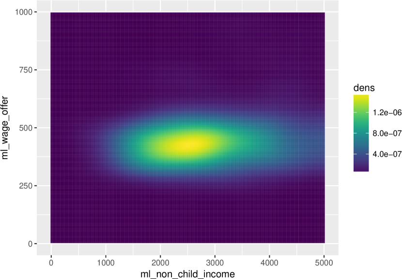
Figure 1: SPS model: original density for boys

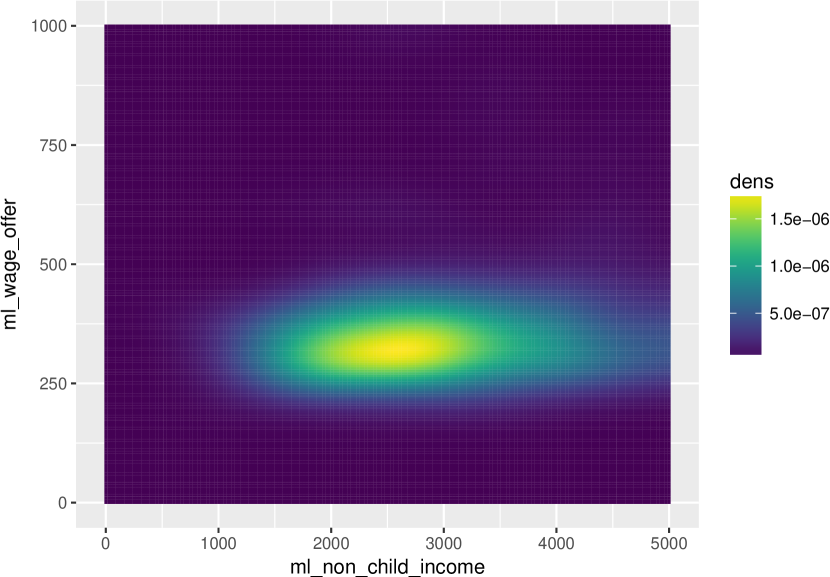
Figure 2: SPS model: counterfactual density for boys

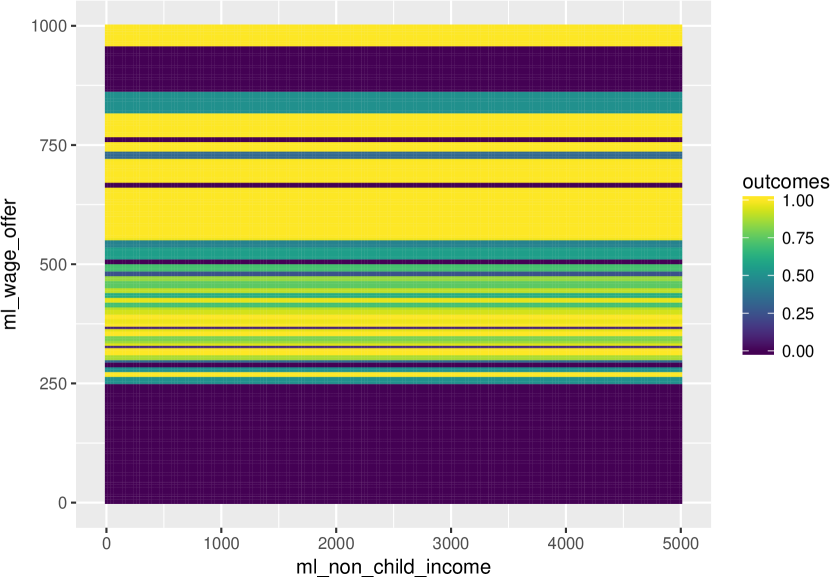
Figure 3: SPS: regression function

Figures 1, 2, and 3 provide some intuition for how SPS works in practice. Figure 1 shows the bivariate density of child wage offers in the held out portion of the control group on the y-axis and non-child income on the x-axis. Figure 2 shows how the model predicts the effect of the TAYSSIR grant. Effective child wage offers decrease, shifting the density down, and non-child income is increased slightly, moving density slightly right.

The impact of this shift depends on the non-parametric regression of enrollment as a function of child wage offer and non-child income in the portion of the control group (non-holdout) available to predictors, which is depicted in Figure 3. The plot shows that non-child income has little association with enrollment conditional on a child’s wage offer. child wage offers do matter, however, particularly in the region where probability mass is being moved.

Table 13 shows that the SPS approach tends to overstate the magnitude of treatment effects. Relative to age-sex based extrapolation from PROGRESA, SPS is only slightly better in cost-adjusted enrollment gain terms than making all children in Morocco eligible for TAYSSIR grants. We think this is because the non-parametric second step is simply too volatile, despite having been regularized by cross validation based bandwidth selection.

5.5 Method 4. Dynamic Parametric Structural

Model

Our Dynamic Parametric Structural (DPS) model is largely based on Attanasio et al. (2012), with a few modifications made to fit data availability and improve in-sample fit in our contexts, following standard practice (see e.g. Wolpin (2013)). The main dynamic features of the model are (1) a finite horizon - children can only be enrolled until age 17 and so can only accumulate subsidies up to this point and (2) persistence of education choices - the flow utility of enrollment is affected by the number of years the child is behind her age-appropriate grade level. Uniquely among our methods, the DPS model allows modeling of the entire subsidy schedule by age.

Flow utility

The in-period utility for child $i$ at age $a$ in school and work are $u^{S}_{ia}$ and $u^{W}_{ia}$, respectively:

$$\begin{array}[]{ l }{u_{ia}^{S}=\gamma\delta g_{ia}+\mu_{i}+\psi^{\prime}z_{ia}+b^{\prime}\cdot\text{yrs\_behind}_{ia}+1\left(p_{ia}=1\right)\beta^{p}x_{ia}^{p}+1\left(s_{ia}=1\right)\beta^{s}x_{ia}^{s}+\varepsilon_{ia}}\\ {u_{ia}^{W}=\delta w_{ia}}\end{array}$$

$g_{ia}$ represents the grant $i$ is entitled to given her completed years of schooling and other characteristics (for example gender). $\mu_{i}$ is a child-specific shifter to the preference for enrollment, drawn from a discrete distribution with $K$ points of support. We will refer to each point of support as an unobserved child “type”. In practice, we estimate the model with three types. $z_{ia}$ includes other observed covariates affecting preference for enrollment. Specifically it includes $a$ and a dummy variable for whether $i$’s father received any formal schooling. $yrs\_behind_{ia}$ is a three-element vector of dummy variables with indicators for being behind grade level by 1 year, 2 years, or $\geq 3$ years. $p_{ia}$ is a dummy variable measuring whether $i$’s years of schooling at age $a$ make her eligible for primary school and $x^{p}_{ia}$ measures distance to school, proxying for cost of attendance. $s_{ia}$ is a dummy variable equal to one if $i$’s years of schooling make her eligible for secondary school and $x^{s}_{ia}$ is a constant. $e_{ia}$ is $i$’s wage offer. $\varepsilon_{ia}$ is an IID idiosyncratic shock to the utility of $i$’s attending school at age $a$, which follows the logistic distribution.

We allow some of the coefficients to vary by $i$’s sex. In particular, $\beta^{s}$ and the component of $\psi$ multiplying age vary by gender. The unobserved type probability also depends on the sex of the child.

Wage offer

Log wage offers are computed according to the same sparse linear regression representation equation described in assumption SPS3 of the SPS model. The only difference is that in the SPS model predicted values from the LASSO regression are treated as estimates of the true wage offer. In the DPS model, agents are assumed to use the same predicted values as the econometrician.

Terminal value

The value of having accumulated $ed_{i18}$ years of school in the terminal period (when the child is 18) is given below.

$$V\left(ed_{i,18}\right)=\frac{\alpha_{1}}{1+\exp\left(-\alpha_{2}ed_{i,18}\right)}+\alpha_{3}\cdot 1\{ed_{i,18}\geq sec\}.$$

$\alpha_{3}$ measures the additional value of having completed secondary school, measured by $ed_{i,18}$ being greater than the last year of secondary school, $sec$.

Value functions

The value of choosing to have $i$ attend school after having completed $ed_{ia}$ years of education by age $a$ is:

$$V_{ia}^{S}\left(ed_{ia}\right)=u_{ia}^{S}+\beta\{p_{a}^{S} \left(ed_{ia}+1\right)\mathbb{E}\,\max\left[V_{i,a+1}^{S}\left(ed_{ia}+1\right),V_{i,a+1}^{\mathrm{W}}\left(ed_{ia}+1\right)\right]$$

$$+\left(1-p_{a}^{S}\left(ed_{it}+1\right)\right)\mathbb{E}\,\max\left[V_{i,a+1}^{S}\left(ed_{ia}\right),V_{i,a+1}^{W}\left(ed_{it}\right)\right]\}.$$ (4)

We implicitly condition on covariates $W_{ia}$ redefined as $W_{ia}\setminus ed_{ia}$ and $\mu_{i}$. $p^{s}_{a}(ed)$ is the probability of successfully passing grade $ed$ at age $a$ conditional on enrolling. We estimate it non-parametrically, outside the model (like the wage offer function). If $i$ successfully passes the grade, she expects to receive the maximum of the value of enrolling or choosing to work in the next year with her education equal to $ed_{ia}+1$. The expectation is taken over possible realizations of the $\varepsilon_{i,a+1}$ shock. If $i$ does not pass, she expects to get the maximum of the value of enrolling/working being one year older and with education still equal to $ed_{ia}$. The term in braces in equation 4 is thus the next-period expected value. From the point of view of this period, the expected value is discounted by $\beta$ which we set equal to 0.95, following AMS. We add the flow utility of being enrolled to complete the definition of the value function when enrolling. The value of having $i$ work this period is simpler since $ed_{ia}$ stays fixed:

$$V_{it}^{W}\left(ed_{ia}\right)=u_{it}^{W}+\beta\mathbb{E}\,\max\left\{V_{i,a+1}^{S}\left(ed_{ia}\right),V_{i,a+1}^{W}\left(ed_{ia}\right)\right\}.$$

Given a set of parameters, we solve for the outputs each value function (enroll, work) for of all possible combinations of age and years of education completed by backward induction, beginning by calculating the terminal value for each set of candidate parameters.

Likelihood

With the value function in hand and the logistic error distribution assumption, it is straightforward to compute the likelihood of each child’s being enrolled given observed characteristics $W_{i}$ and unobserved type $\mu_{i}$: $\Pr(Y_{i}=1|W_{i},\mu_{i}=\mu_{k})$. The full likelihood associated with $Y_{i}=1$ is given by:

$$\Pr(Y_{i}=1|W_{i})=\sum_{k=1}^{K}\frac{1}{1+\exp(V^{W}_{it}(ed_{i}|\mu_{k},W_{i})-V^{S}_{it}(ed_{i}|\mu_{k},W_{i}))}\Pr(\mu_{i}=\mu_{k}|W_{i},\mu_{k}).$$ (5)

Since the utility shock $\varepsilon_{i}$ is IID across time and individuals, we could in principle derive the conditional type probability as a function of the history of characteristics and education decisions of $i$ starting at the age when $i$’s enrollment was first considered ($min\_a$): $(W_{i,a-1},\ldots,W_{i,min\_a})$ and $(Y_{i,a-1},\ldots,Y_{i,min\_a})$ respectively:

$$\Pr(\mu_{i}=\mu_{k}|(Y_{i,a-1},\ldots,Y_{i,min\_a}),(W_{i,a-1},\ldots,W_{i,min\_a}))$$

$$=\frac{\Pr(Y_{ia}|W_{ia},\mu_{i}=\mu_{k})\cdots\Pr(Y_{i,min\_a}|W_{i,\min\_a},\mu_{i}=\mu_{k})\Pr(\mu_{k})}{\sum_{k=1}^{K}\Pr(Y_{ia}|W_{ia},\mu_{i}=\mu_{k})\cdots\Pr(Y_{i,min\_a}|W_{i,\min\_a},\mu_{i}=\mu_{k})\Pr(\mu_{k})}.$$ (6)

Actually estimating (6) is infeasible, however, since it requires knowledge of the full histories $(W_{i,a-1},\ldots,W_{i,min\_a})$ and $(Y_{i,a-1},\ldots,Y_{i,min\_a})$ and, furthermore, would be very high-dimensional.

Following Todd and Wolpin (2006), we instead use a multinomial logit approximation:

$$\Pr(\mu_{i}=\mu_{k}|(Y_{i,a-1},\ldots,Y_{i,min\_a}),(W_{i,a-1},\ldots,W_{i,min\_a}))$$

$$\approx\Pr(\mu_{i}=\mu_{k}|a,ed_{ia},gender,father\_ed)$$

$$\ \ \ \approx\frac{\exp(\beta^{\mu}_{k}\cdot(1,a,ed_{ia},gender,father\_ed))}{1+\sum_{k}\exp(\beta^{\mu}_{k}\cdot(1,a,ed_{ia},gender,father\_ed)},k\in{1\ldots,K-1}$$

Age proxies for the length of the history, $ed_{ia}$ for $(Y_{i,a-1},\ldots,Y_{i,min\_a})$ and $gender$ and $father\_ed$ for $(W_{i,a-1},\ldots,W_{i,min\_a})$ (specifically $W_{i,min\_a}$). Importantly, $ed_{ia}$ is excluded from flow utility so there is independent variation to identify the conditional type probabilities. We estimate the parameters described above, along with the support points $(\mu_{1},\cdots,\mu_{K})$ by maximum likelihood.

5.5.1 Results

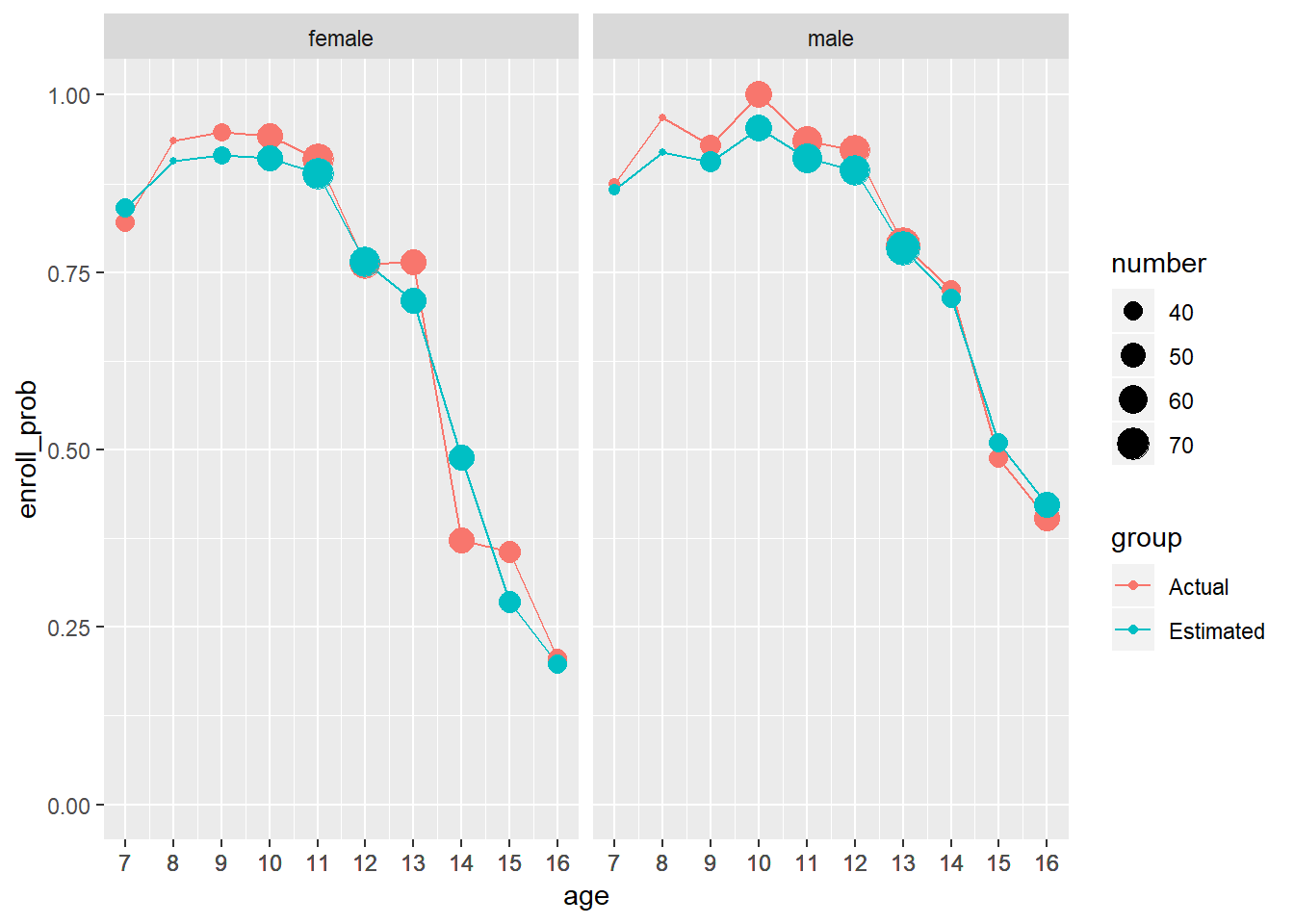
Figure 4: DPS: in-sample fit by age

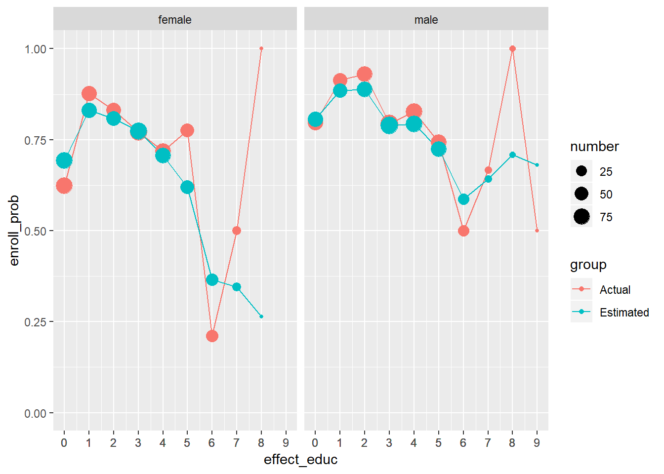
Figure 5: DPS: in-sample fit by years of education completed

Figures 4 and 5 show that the model fits well in the portion of the Moroccan control group made available to predictors. Figure 4 shows the fit to enrollment rates by age. The size of each point on the graph representing the sample size in that age-sex stratum. The model captures delayed entry into school, near-universal enrollment at young ages, and the sharp drop in enrollment for teenagers. Figure 5 illustrates the fit by number of years of education completed. It captures the drop in enrollment at the transition to secondary school (year 7 in Morocco).

Table 14 shows the results from using the DPS model to predict the effect of the TAYSSIR program. For all but a tiny fraction of the Moroccan holdout sample, predicted enrollment gains - while reasonable - are too small to exceed the cost-effectiveness threshold. We show this visually in Figure 6, plotting the CDF of predicted treatment effects due to observables. A key point from Table 14 is how close TAYSSIR is to being non-cost-effective for any child. Age-sex based extrapolation from PROGRESA only provides a small, statistically insignificant increase in welfare relative to DPS’s no-treatment recommendation.

6 Conclusion

We develop a decision-based approach to comparing the relative performance of methods for generating counterfactual predictions that are then used to make policy recommendations. We consider a social planner who is operating in a target context and is seeking recommendations on what policy to choose from a set of feasible options. The richness of the space of policy options determines the nature of the recommendations being sought — e.g., whether a simple up-or-down recommendation to treat everyone or no one, or a more refined recommendation about who should be treated and who not. Recommendations could be based on econometric estimates, whether reduced form or structural, or expert opinions. Our leading application is one where the planner maximizes a linear welfare objective in assigning treatments on the basis of available covariate information. In this case, the success of a method for generating recommendations depends on how accurately it can predict conditional treatment effects in the target context.

We define a welfare contrast to use for conducting an ex post analysis of how well different methods performed with respect to the planner’s goals. We estimate this welfare contrast by using experimental data that reveals how a treatment affects the outcome distribution in the target population. The welfare contrast is straightforward to compute, and it allows us to judge whether one method outperforms another in a manner that is statistically significant.

We provide an empirical illustration that considers a planner seeking a recommendation on how to implement program using conditional cash transfers (CCTs) to boost school enrollment in Morocco. The data available for generating recommendations include a randomized evaluation of CCTs in Mexico as well as data from Moroccan households under the status quo ex ante, in which no CCTs have been applied. We generate recommendations from reduced form methods and structural models. We then perform an ex post evaluation of these methods using data from a randomized evaluation of CCTs in Morocco. We view this toy example as helping build intuition for how to specify methods to evaluate in a full-featured empirical portion of the paper including the contexts from Banerjee et al. (2017) which we will pre-specify.

We see this exercise as making three contributions. First, as our application attempts to show, it provides a clear framework to assess internal validity versus external validity trade-offs. In particular, our application allows us to assess how robust and internally valid estimates from external contexts fare relative to within-context estimates that may be biased due to model misspecification (Pritchett and Sandefur, 2013). Second, it provides a principled basis for assessing the performance of different methods by tying the assessment to welfare considerations. This is important, because different objective functions can imply different rank orderings of methods. Our approach thus forces one to first consider the welfare objective so as to be clear about the relevant objective. Third, we show that each experiment or observational study may contain much more decision-relevant information than would be contained in a single treatment effect estimate.

We are undertaking a number of extensions to what we have done here. Model selection or model averaging approaches based on our welfare criteria may lead to better predictions. We also plan to work with evidence bases that include more external contexts. In doing so, we would want to account for site selection, as per Allcott (2015b) and Gechter and Meager (2018).

Appendix A Proofs

Proof of Proposition 1.

By the weak law of large numbers, Slutsky’s theorem, and conditions C2 and C3, $\hat{\Delta}^{g}_{lm}$ has the same limit as

$$\tilde{\Delta}^{g}_{lm}= \frac{1}{N}\sum_{i=1}^{N}\frac{T_{i}}{p(W_{i})}\left(\pi_{l}(W_{i})-\pi_{m}(W_{i})\right)g(Y^{P}_{i}(1))$$

$$-\frac{1}{N}\sum_{i=1}^{N}\frac{1-T_{i}}{1-p(W_{i})}\left(\pi_{l}(W_{i})-\pi_{m}(W_{i})\right)g(Y^{P}_{i}(0)).$$

Take the first term on the right-hand side. By the weak law of large numbers, iterated expectations, and condition C1,

$$\frac{1}{N}\sum_{i=1}^{N}\frac{T_{i}}{p(W_{i})}\left(\pi_{l}(W_{i})-\pi_{m}(W_{i})\right)g(Y^{P}_{i}(1))$$

$$\overset{p}{\rightarrow}\mathbb{E}\,\left[\mathbb{E}\,[T_{i}|W]\frac{1}{p(W)}\mathbb{E}\,[\left(\pi_{l}(W_{i})-\pi_{m}(W_{i})\right)g(Y^{P}_{i}(1))|W]\right]$$

$$=\mathbb{E}\,\left[\left(\pi_{l}(W_{i})-\pi_{m}(W_{i})\right)g(Y^{P}_{i}(1))\right],$$

and similar for the second term. Thus as $N\rightarrow\infty$, $\mathbb{E}\,[\hat{\Delta}^{g}_{lm}-\Delta^{g}_{lm}]\overset{p}{\rightarrow}0$. Having established that $\hat{\Delta}^{g}_{lm}$ is asymptotically unbiased for $\Delta^{g}_{lm}$, inference follows from the usual generalized method of moments results (Newey and McFadden, 1994; Lunceford and Davidian, 2004). To see this, first note that $\hat{\Delta}^{g}_{lm}=\hat{\delta}_{1}-\hat{\delta}_{0}$ for $(\hat{\delta}_{1},\hat{\delta}_{0})$ that solve the score equations

$$\sum_{i=1}^{N}\psi_{1}(\hat{\delta}_{1})=0 \text{ and }\sum_{i=1}^{N}\psi_{0}(\hat{\delta}_{0})=0,$$

$$\text{where }\psi_{1}(\hat{\delta}_{1})=\frac{T_{i}\left[(\pi_{l}(W_{i})-\pi_{m}(W_{i}))g(Y_{i})-\hat{\delta}_{1}\right]}{p(W_{i})},$$

$$\text{ and }\psi_{0}(\hat{\delta}_{0})=\frac{(1-T_{i})\left[(\pi_{l}(W_{i})-\pi_{m}(W_{i}))g(Y_{i})-\hat{\delta}_{0}\right]}{1-p(W_{i})}.$$

Then, given random sampling, bounded first and second moments, and conditions C1-C2, we have

$$\frac{\sqrt{N}\left(\hat{\Delta}^{g}_{lm}-\Delta^{g}_{lm}\right)}{\sqrt{V_{\Delta^{g}_{lm}}}}\overset{d}{\rightarrow}N(0,1),$$ (7)

where

$$V_{\Delta^{g}_{lm}} =\mathbb{E}\,[\psi_{1}(\delta_{1})^{2}+\psi_{0}(\delta_{0})^{2}]$$

$$=\mathbb{E}\,\left\{\frac{\left[(\pi_{l}(W_{i})-\pi_{m}(W_{i}))g(Y_{i}^{P}(1))-\delta_{1}\right]^{2}}{p(W_{i})}+\frac{\left[(\pi_{l}(W_{i})-\pi_{m}(W_{i}))g(Y_{i}^{P}(0))-\delta_{0}\right]^{2}}{1-p(W_{i})}\right\},$$

with $\delta_{t}=\mathbb{E}\,[(\pi_{l}(W_{i})-\pi_{m}(W_{i}))g(Y_{i}^{P}(t))]$. Then, by the same conditions for which $\hat{\Delta}^{g}_{lm}$ is consistent for $\Delta^{g}_{lm}$, $\hat{V}_{\Delta^{g}_{lm}}$ is consistent for $V_{\Delta^{g}_{lm}}$. ∎

Figure 6: DPS predicted treatment effect, no cost-effectiveness adjustment

Age	Male	Treated	Control	CATE	PEN_ub	PNE_ub
6.00	1.00	0.93	0.91	0.02	0.09	0.07
7.00	1.00	0.96	0.96	-0.00	0.04	0.04
8.00	1.00	0.97	0.96	0.01	0.04	0.03
9.00	1.00	0.98	0.96	0.02	0.04	0.02
10.00	1.00	0.97	0.96	0.01	0.04	0.03
11.00	1.00	0.96	0.93	0.03	0.07	0.04
12.00	1.00	0.91	0.86	0.05	0.14	0.09
13.00	1.00	0.83	0.76	0.07	0.24	0.17
14.00	1.00	0.74	0.60	0.14	0.40	0.26
15.00	1.00	0.53	0.46	0.07	0.53	0.46
16.00	1.00	0.35	0.32	0.03	0.35	0.32
6.00	0.00	0.90	0.89	0.01	0.11	0.10
7.00	0.00	0.95	0.95	0.00	0.05	0.05
8.00	0.00	0.96	0.96	0.00	0.04	0.04
9.00	0.00	0.97	0.95	0.01	0.05	0.03
10.00	0.00	0.97	0.96	0.00	0.04	0.03
11.00	0.00	0.94	0.92	0.03	0.08	0.06
12.00	0.00	0.88	0.79	0.09	0.21	0.12
13.00	0.00	0.74	0.68	0.05	0.32	0.26
14.00	0.00	0.65	0.52	0.13	0.48	0.35
15.00	0.00	0.41	0.35	0.06	0.41	0.35
16.00	0.00	0.33	0.25	0.07	0.33	0.25

Table 1: Age-sex Outcomes for Mexico

Age	Boys treated	Boys control	Girls treated	Girls control
6.00	0.84	0.91	0.82	0.89
7.00	0.87	0.96	0.87	0.95
8.00	0.85	0.96	0.85	0.96
9.00	0.86	0.96	0.85	0.95
10.00	0.83	0.96	0.82	0.96
11.00	0.82	0.93	0.80	0.92
12.00	0.77	0.86	0.75	0.79
13.00	0.70	0.76	0.63	0.68
14.00	0.63	0.60	0.56	0.52
15.00	0.45	0.46	0.35	0.35
16.00	0.30	0.32	0.28	0.25

Table 2: Adjusted Age-sex Outcomes for Mexico

	w/ CE	w/o CE
Share treated (age-sex)	0.126	0.966
Share treated (all)	1.000	1.000
Enrollment difference	-0.035	-0.005
SE enroll. diff.	0.011	0.004
Welfare difference	0.065	-0.002
SE welfare diff.	0.010	0.004

Table 3: Welfare comparison for age-sex extrapolation vs. treat all

Variable	Importance Y1	Importance Y0
ml_base_enrolled	0.21	0.19
ml_age	0.33	0.32
ml_n_child	0.02	0.01
ml_male	0.01	0.01
ml_hh_head_male	0.00	0.00
ml_single_parent	0.00	0.00
ml_al_father	0.00	0.01
ml_al_mother	0.00	0.00
ml_lw_father	0.00	0.00
ml_lw_mother	0.00	0.00
ml_literacy	0.03	0.04
ml_n_total	0.01	0.01
ml_yrs_educ	0.16	0.18
ml_hh_head_edu	0.07	0.07
ml_father_educ	0.05	0.04
ml_mother_educ	0.07	0.08
ml_base_enrolled_mi	0.01	0.01
ml_male_mi	0.00	0.00
ml_al_father_mi	0.00	0.00
ml_al_mother_mi	0.00	0.00
ml_literacy_mi	0.01	0.01
ml_yrs_educ_mi	0.01	0.01
ml_father_educ_mi	0.01	0.00
ml_mother_educ_mi	0.00	0.00
ml_hh_monthly_consump	0.00	0.00
ml_n_child_mi	0.00	0.00
ml_lw_father_mi	0.00	0.00
ml_hh_monthly_consump_mi	0.00	0.00

Table 4: GRF variable importance: no cost-effectiveness adjustment

Variable	Importance Y1	Importance Y0
ml_base_enrolled	0.19	0.19
ml_age	0.28	0.27
ml_n_child	0.02	0.01
ml_male	0.01	0.01
ml_hh_head_male	0.01	0.00
ml_single_parent	0.00	0.00
ml_al_father	0.01	0.01
ml_al_mother	0.03	0.03
ml_lw_father	0.00	0.00
ml_lw_mother	0.01	0.01
ml_literacy	0.03	0.04
ml_n_total	0.01	0.01
ml_yrs_educ	0.16	0.15
ml_hh_head_edu	0.08	0.08
ml_father_educ	0.05	0.04
ml_mother_educ	0.06	0.08
ml_base_enrolled_mi	0.01	0.01
ml_male_mi	0.01	0.00
ml_al_father_mi	0.00	0.00
ml_al_mother_mi	0.00	0.00
ml_literacy_mi	0.01	0.02
ml_yrs_educ_mi	0.01	0.02
ml_father_educ_mi	0.00	0.00
ml_mother_educ_mi	0.01	0.00

Table 5: GRF variable importance: Y1 adjusted for cost-effectiveness

Age	Male	Avg. TE	Min. TE	Max TE	SD TE
6.00	1.00	-0.06	-0.20	0.08	0.06
7.00	1.00	-0.05	-0.18	0.12	0.06
8.00	1.00	0.03	-0.07	0.12	0.04
9.00	1.00	0.06	-0.04	0.16	0.04
10.00	1.00	0.06	-0.10	0.16	0.03
11.00	1.00	0.04	-0.07	0.15	0.03
12.00	1.00	0.05	-0.14	0.18	0.05
13.00	1.00	0.07	-0.19	0.19	0.09
14.00	1.00	0.15	-0.11	0.41	0.08
15.00	1.00	0.20	-0.16	0.45	0.11
16.00	1.00	0.09	-0.26	0.32	0.14

Table 6: GRF CATE predictions for Morocco: Boys, no cost-effectiveness adjustment

Age	Male	Avg. TE	Min. TE	Max TE	SD TE
6.00	1.00	-0.04	-0.21	0.14	0.05
7.00	1.00	-0.02	-0.14	0.12	0.05
8.00	1.00	0.01	-0.09	0.17	0.05
9.00	1.00	0.03	-0.12	0.17	0.06
10.00	1.00	0.03	-0.09	0.14	0.04
11.00	1.00	0.02	-0.08	0.15	0.03
12.00	1.00	0.04	-0.14	0.16	0.04
13.00	1.00	0.05	-0.18	0.19	0.09
14.00	1.00	0.14	-0.08	0.41	0.09
15.00	1.00	0.14	-0.12	0.39	0.13
16.00	1.00	0.06	-0.18	0.38	0.11

Table 7: GRF CATE predictions for Morocco: Girls, no cost-effectiveness adjustment

Age	Male	Avg. Adj. TE	Min. Adj. TE	Max Adj. TE	SD Adj. TE
6.00	1.00	-0.10	-0.22	0.05	0.06
7.00	1.00	-0.08	-0.18	0.06	0.05
8.00	1.00	-0.03	-0.11	0.09	0.03
9.00	1.00	-0.00	-0.07	0.12	0.04
10.00	1.00	-0.02	-0.13	0.09	0.03
11.00	1.00	-0.03	-0.12	0.08	0.03
12.00	1.00	-0.01	-0.16	0.11	0.04
13.00	1.00	0.01	-0.24	0.11	0.07
14.00	1.00	0.07	-0.11	0.26	0.06
15.00	1.00	0.14	-0.17	0.33	0.10
16.00	1.00	0.05	-0.23	0.23	0.11

Table 8: GRF CATE predictions for Morocco: Boys, adjusted for cost-effectiveness

Age	Male	Avg. Adj. TE	Min. Adj. TE	Max Adj. TE	SD Adj. TE
6.00	1.00	-0.08	-0.24	0.06	0.04
7.00	1.00	-0.06	-0.16	0.05	0.04
8.00	1.00	-0.05	-0.17	0.09	0.05
9.00	1.00	-0.04	-0.14	0.11	0.05
10.00	1.00	-0.05	-0.14	0.04	0.03
11.00	1.00	-0.05	-0.13	0.12	0.02
12.00	1.00	-0.03	-0.16	0.05	0.04
13.00	1.00	-0.01	-0.22	0.10	0.07
14.00	1.00	0.07	-0.08	0.28	0.06
15.00	1.00	0.09	-0.12	0.31	0.11
16.00	1.00	0.02	-0.21	0.27	0.09

Table 9: GRF CATE predictions for Morocco: Girls, adjusted for cost-effectiveness

Age	Girls share	Girls treat rate	Boys share	Boys treat rate
6.00	0.05	0.18	0.06	0.17
7.00	0.07	0.28	0.07	0.23
8.00	0.09	0.55	0.08	0.81
9.00	0.08	0.73	0.08	0.94
10.00	0.10	0.86	0.12	0.94
11.00	0.12	0.78	0.12	0.88
12.00	0.13	0.86	0.13	0.91
13.00	0.12	0.71	0.12	0.83
14.00	0.09	0.95	0.10	0.98
15.00	0.09	0.91	0.08	0.94
16.00	0.06	0.80	0.05	0.79

Table 10: GRF treatment rates for Morocco, no cost-effectiveness adjustment

Age	Girls share	Girls treat rate	Boys share	Boys treat rate
6.00	0.05	0.05	0.06	0.04
7.00	0.07	0.09	0.07	0.04
8.00	0.09	0.14	0.08	0.20
9.00	0.08	0.27	0.08	0.41
10.00	0.10	0.09	0.12	0.27
11.00	0.12	0.03	0.12	0.12
12.00	0.13	0.19	0.13	0.39
13.00	0.12	0.51	0.12	0.62
14.00	0.09	0.89	0.10	0.93
15.00	0.09	0.79	0.08	0.91
16.00	0.06	0.58	0.05	0.73

Table 11: GRF treatment rates for Morocco, adjusted for cost-effectiveness

	w/ CE	w/o CE
Share treated (GRF)	0.377	0.772
Share treated (age-sex)	0.126	0.966
Enrollment difference	0.011	-0.002
SE enroll. diff.	0.010	0.008
Welfare difference	-0.018	0.014
SE welfare diff.	0.009	0.008

Table 12: Welfare comparison for GRF vs. age-sex extrapolation

	w/ CE
Share treated (SPS)	0.447
Share treated (age-sex)	0.126
Enrollment difference	-0.018
SE enroll. diff.	0.010
Welfare difference	-0.046
SE welfare diff.	0.009

Table 13: Welfare comparison for SPS vs. age-sex extrapolation

	w/ CE
Share treated (DPS)	0.001
Share treated (age-sex)	0.151
Enrollment difference	-0.017
SE enroll. diff.	0.008
Welfare difference	-0.004
SE welfare diff.	0.008

Table 14: Welfare comparison for DPS vs. age-sex extrapolation

References

- Allcott (2015a) Allcott, H. (2015a). Site Selection Bias in Program Evaluation. Quarterly Journal of Economics 130(3), 1117–1165.
- Allcott (2015b) Allcott, H. (2015b). Site Selection Bias in Program Evaluation. The Quarterly Journal of Economics 130(3), 1117–1165.
- Andrews and Oster (2017) Andrews, I. and E. Oster (2017). WEIGHTING FOR EXTERNAL VALIDITY.
- Aronow and Samii (2017) Aronow, P. M. and C. Samii (2017). Estimating average causal effects under general interference, with application to a social network experiment. Annals of Applied Statistics 11(4), 1912–1947.
- Arrow (1972) Arrow, K. J. (1972). The Value of and Demand for Information. In C. McGuire and R. Radner (Eds.), Decision and Organization. A Volume in Honor of Jacob Marschak (Amsterdam ed.)., Chapter 6, pp. 131–140. North-Holland.
- Athey et al. (2019) Athey, S., J. Tibshirani, and S. Wager (2019). Generalized random forests. The Annals of Statistics 47(2), 1148–1178.
- Athey and Wager (2017) Athey, S. and S. Wager (2017). Efficient Policy Learning.
- Attanasio et al. (2012) Attanasio, O., C. Meghir, and A. Santiago (2012). Education Choices in Mexico: Using a Structural Model and a Randomised Experiment to Evaluate PROGRESA. Review of Economic Studies 79(1), 37–66.
- Banerjee et al. (2016) Banerjee, A., S. Chassang, and E. Snowberg (2016). Decision Theoretic Approaches to Experiment Design and External Validity. In Handbook of Field Experiments, forthcoming.
- Banerjee et al. (2017) Banerjee, A., R. Hanna, G. Kreindler, and B. A. Olken (2017). Debunking the Stereotype of the Lazy Welfare Recipient: Evidence from Cash Transfer Programs Worldwide. The World Bank Research Observer 32(2), 155–184.
- Behrman et al. (2005) Behrman, J. R., P. Sengupta, and P. E. Todd (2005, oct). Progressing through PROGRESA: An Impact Assessment of a School Subsidy Experiment in Rural Mexico. Economic Development and Cultural Change 54(1), 237–275.
- Belloni et al. (2012) Belloni, A., D. Chen, V. Chernozhukov, and C. Hansen (2012). Sparse Models and Methods for Optimal Instruments with an Application to Eminent Domain. Econometrica 80(6), 2369–2429.
- Benhassine et al. (2015) Benhassine, N., F. Devoto, E. Duflo, P. Dupas, and V. Pouliquen (2015). Turning a shove into a nudge? A ”labeled cash transfer” for education. American Economic Journal: Economic Policy 7(3), 1–48.
- Bhattacharya and Dupas (2012) Bhattacharya, D. and P. Dupas (2012). Inferring welfare maximizing treatment assignment under budget constraints. Journal of Econometrics 167(1), 168–196.
- Cox (1958) Cox, D. R. (1958). Planning of Experiments. Wiley.
- De Janvry and Sadoulet (2006) De Janvry, A. and E. Sadoulet (2006, mar). Making conditional cash transfer programs more efficient: designing for maximum effect of the conditionality. The World Bank Economic Review 20(1), 1.
- Dehejia et al. (2016) Dehejia, R., C. Pop-Eleches, and C. Samii (2016). From local to global: External validity in a fertility natural experiment.
- Dehejia et al. (2017) Dehejia, R., C. Pop-Eleches, and C. Samii (2017). From Local to Global: External Validity in a Fertility Natural Experiment. NBER Working Paper 21459.
- Dehejia (2003) Dehejia, R. H. (2003, jan). Was There a Riverside Miracle? A Hierarchical Framework for Evaluating Programs With Grouped Data. Journal of Business and Economic Statistics 21(1), 1–11.
- Dehejia (2005) Dehejia, R. H. (2005, apr). Program evaluation as a decision problem. Journal of Econometrics 125(1-2), 141–173.
- Dehejia (2008) Dehejia, R. H. (2008). When is ATE enough? Risk aversion and inequality aversion in evaluating training programs. Advances in Econometrics 21, 263–287.
- DellaVigna and Pope (2017) DellaVigna, S. and D. Pope (2017). Predicting Experimental Results: Who Knows What? Journal of Political Economy, forthcoming.
- Dhaliwal et al. (2011) Dhaliwal, I., E. Duflo, and R. Glennerster (2011). Comparative Cost-Effectiveness Analysis to Inform Policy in Developing Countries: A General Framework with Applications for Education.
- Diebold (2015) Diebold, F. X. (2015). Comparing Predictive Accuracy, Twenty Years Later: A Personal Perspective on the Use and Abuse of Diebold–Mariano Tests. Journal of Business & Economic Statistics 33(1), 1–1.
- Diebold and Mariano (1995) Diebold, F. X. and R. S. Mariano (1995). Comparing Predictive Accuracy. Journal of Business & Economic Statistics 13(3), 253.
- Duflo et al. (2012) Duflo, E., R. Hanna, and S. Ryan (2012). Incentives work: Getting teachers to come to school. The American Economic Review 102(4), 1241–1278.
- Garber and Phelps (1997) Garber, A. M. and C. E. Phelps (1997). Economic foundations of cost-effectiveness analysis. Journal of Health Economics 16(1), 1–31.
- Garcia and Saavedra (2017) Garcia, S. and J. Saavedra (2017). Educational impacts and cost-effectiveness of conditional cash transfer programs in developing countries: A meta-analysis. NBER Working Paper No. 23594.
- Gechter (2016) Gechter, M. (2016). Generalizing the Results from Social Experiments: Theory and Evidence from Mexico and India. Working Paper.
- Gechter and Meager (2018) Gechter, M. and R. Meager (2018). Incorporating Experimental and Observational Studies in Meta-Analysis. Working Paper.
- Granger and Machina (2006) Granger, C. and M. Machina (2006). Forecasting and decision theory. Handbook of economic forecasting 1(05), 81–98.
- Hansen et al. (2011) Hansen, P. R., A. Lunde, and J. M. Nason (2011). The Model Confidence Set. Econometrica 79(2), 453–497.
- Hayfield and Racine (2008) Hayfield, T. and J. S. Racine (2008). Nonparametric econometrics: The np package. Journal of Statistical Software 27(5).
- Hirano et al. (2003) Hirano, K., G. Imbens, and G. Ridder (2003). Efficient estimation of average treatment effects using the estimated propensity score. Econometrica 71(4), 1161–1189.
- Hirano and Porter (2009) Hirano, K. and J. R. Porter (2009). Asymptotics for Statistical Treatment Rules. Econometrica 77(5), 1683–1701.
- Hirano and Porter (2019) Hirano, K. and J. R. Porter (2019). Statistical Decision Rules in Econometrics. In Handbook of Econometrics, Volume 7.
- Hotz et al. (2005) Hotz, V. J., G. Imbens, and J. Mortimer (2005). Predicting the Efficacy of Future Training Programs Using Past Experiences at Other Locations. Journal of Econometrics 125, 241–270.
- Hudgens and Halloran (2008) Hudgens, M. G. and M. E. Halloran (2008). Toward causal inference with interference. Journal of the American Statistical Association 103(482), 832–842.
- Imai and Strauss (2011) Imai, K. and A. Strauss (2011). Estimation of heterogeneous treatment effects from randomized experiments, with application to the optimal planning of the get-out-the-vote campaign. Political Analysis 19(1), 1–19.
- Imbens and Wooldridge (2009) Imbens, G. W. G. and J. M. Wooldridge (2009). Recent developments in the econometrics of program evaluation. Journal of Economic Literature 47(1), 5–86.
- Keane et al. (2011) Keane, M. P., P. E. Todd, and K. I. Wolpin (2011). The Structural Estimation of Behavioral Models: Discrete Choice Dynamic Programming Methods and Applications. Handbook of Labor Economics, Volume 4 4(2), 331–461.
- Keane and Wolpin (2007) Keane, M. P. and K. I. Wolpin (2007, dec). Exploring the usefulness of a nonrandom holdout sample for model validation: welfare effects on female behavior. International Economic Review 48(4), 1351–1378.
- Kitagawa and Tetenov (2017) Kitagawa, T. and A. Tetenov (2017). Who should be treated? Empirical welfare maximization methods for treatment choice. Econometrica, Forthcoming.
- Lunceford and Davidian (2004) Lunceford, J. K. and M. Davidian (2004). Stratification and weighting via the propensity score in estimation of causal treatment effects: A comparative study. Statistics in Medicine 23(19), 2937–2960.
- Mammen et al. (2012) Mammen, E., C. Rothe, and M. Schienle (2012). Nonparametric regression with nonparametrically generated covariates. Annals of Statistics 40(2), 1132–1170.
- Manski (1996) Manski, C. F. (1996). Learning about Treatment Effects from Experiments with Random Assignment of Treatments. The Journal of Human Resources 31(4), 709.
- Manski (2004) Manski, C. F. (2004, jul). Statistical Treatment Rules for Heterogeneous Populations. Econometrica 72(4), 1221–1246.
- Manski (2011) Manski, C. F. (2011). Choosing Treatment Policies Under Ambiguity. Annual Review of Economics 3(1), 25–49.
- Marschak and Miyasawa (1968) Marschak, J. and K. Miyasawa (1968). Economic Comparability of Information Systems. Internal Economic Review 9(2), 137–174.
- Meager (2016) Meager, R. (2016). Understanding the Impact of Microcredit Expansions: A Bayesian Hierarchical Analysis of 7 Randomised Experiments.
- Montenegro and Patrinos (2014) Montenegro, C. E. and H. A. Patrinos (2014). Comparable Estimates of Returns to Schooling Around the World. World Bank Policy Research Working Paper 7020.
- Newey and McFadden (1994) Newey, W. and D. McFadden (1994). Large sample estimation and hypothesis testing. Handbook of econometrics 4, 2111–2245.
- Parker and Vogl (2018) Parker, S. W. and T. Vogl (2018). Do conditional cash transfers improve economic outcomes in the next generation? Evidence from mexico.
- Pesaran and Skouras (2002) Pesaran, M. and S. Skouras (2002). Decision-Based Methods for Forecast Evaluation. In M. Clements and D. Hendry (Eds.), A Companion to Economic Forecasting. Oxford: Blackwell.
- Pritchett and Sandefur (2013) Pritchett, L. and J. Sandefur (2013). Context Matters for Size: Why External Validity Claims and Development Practice Don’t Mix. Journal of Globalization and Development 4(2), 161–197.
- Rubin (1980) Rubin, D. B. (1980). Randomization analysis of experimental data: The Fisher randomization test comment. Journal of the American Statistical Association 75(371), 591–593.
- Schorfheide and Wolpin (2012) Schorfheide, F. and K. I. Wolpin (2012, may). On the Use of Holdout Samples for Model Selection. American Economic Review 102(3), 477–481.
- Schorfheide and Wolpin (2016) Schorfheide, F. and K. I. Wolpin (2016). To Hold Out or Not To Hold Out. Research in Economics, forthcoming.
- Schultz (2004) Schultz, T. P. (2004, jun). School subsidies for the poor: evaluating the Mexican Progresa poverty program. Journal of Development Economics 74(1), 199–250.
- Tetenov (2012) Tetenov, A. (2012). Statistical treatment choice based on asymmetric minimax regret criteria. Journal of Econometrics 166(1), 157–165.
- Todd and Wolpin (2006) Todd, P. E. and K. I. Wolpin (2006). Assessing the impact of a school subsidy program in Mexico: Using a social experiment to validate a dynamic behavioral model of child schooling and fertility. The American Economic Review 96(5), 1384–1417.
- Todd and Wolpin (2008) Todd, P. E. and K. I. Wolpin (2008). Ex ante evaluation of social programs. Annales d’Economie et de Statistique (91/92), 263–291.
- Vivalt (2016) Vivalt, E. (2016). How Much Can We Generalize From Impact Evaluations? Mimeo.
- Vuong (1989) Vuong, Q. (1989). Likelihood Ratio Tests for Model Selection and Non-Nested Hypotheses. Econometrica 57(2), 307–333.
- West (1996) West, K. (1996). Asymptotic inference about predictive ability. Econometrica 64(5), 1067–1084.
- White (2000) White, H. (2000). A reality check for data snooping. Econometrica 68(5), 1097–1126.
- Wolpin (2007) Wolpin, K. (2007, may). Ex Ante Policy Evaluation, Structural Estimation, and Model Selection. The American economic review 97(2), 48–52.
- Wolpin (2013) Wolpin, K. I. (2013). The Limits of Inference Without Theory. The MIT Press.