Optimization over Nonnegative and Convex Polynomials with and without Semidefinite Programming

Abstract

The problem of optimizing over the cone of nonnegative polynomials is a fundamental problem in computational mathematics, with applications to polynomial optimization, control, machine learning, game theory, and combinatorics, among others. A number of breakthrough papers in the early 2000s showed that this problem, long thought to be out of reach, could be tackled by using sum of squares programming. This technique however has proved to be expensive for large-scale problems, as it involves solving large semidefinite programs (SDPs).

In the first part of this thesis, we present two methods for approximately solving large-scale sum of squares programs that dispense altogether with semidefinite programming and only involve solving a sequence of linear or second order cone programs generated in an adaptive fashion. We then focus on the problem of finding tight lower bounds on polynomial optimization problems (POPs), a fundamental task in this area that is most commonly handled through the use of SDP-based sum of squares hierarchies (e.g., due to Lasserre and Parrilo). In contrast to previous approaches, we provide the first theoretical framework for constructing converging hierarchies of lower bounds on POPs whose computation simply requires the ability to multiply certain fixed polynomials together and to check nonnegativity of the coefficients of their product.

In the second part of this thesis, we focus on the theory and applications of the problem of optimizing over convex polynomials, a subcase of the problem of optimizing over nonnegative polynomials. On the theoretical side, we show that the problem of testing whether a cubic polynomial is convex over a box is NP-hard. This result is minimal in the degree of the polynomial and complements previously-known results on checking convexity of a polynomial globally. We also study norms generated by convex forms and provide an SDP hierarchy for optimizing over them. This requires an extension of a result of Reznick on sum of squares representation of positive definite forms to positive definite biforms. On the application side, we study a problem of interest to robotics and motion planning, which involves modeling complex environments with simpler representations. In this setup, we are interested in containing 3D-point clouds within polynomial sublevel sets of minimum volume. We also study two applications in machine learning: the first is multivariate monotone regression, which is motivated by some applications in pricing; the second concerns a specific subclass of optimization problems called difference of convex (DC) programs, which appear naturally in machine learning problems. We show how our techniques can be used to optimally reformulate DC programs in order to speed up some of the best-known algorithms used for solving them.

June 2018 Professor Amir Ali Ahmadi Operations Research and Financial Engineering

Chapter 1 Introduction

This thesis concerns itself broadly with the problem of optimizing over nonnegative polynomials. In its simplest form, this problem involves (i) decision variables that are the coefficients of a multivariate polynomial of a given degree, (ii) an objective function that is linear in the coefficients, (iii) constraints that are affine in the coefficients, and (iv) a constraint that the multivariate polynomial be nonnegative over a closed basic semialgebraic set, i.e., a set defined by a finite number of polynomial inequalities. We write:

$$\min_{\overrightarrow{p}} c(\overrightarrow{p})$$ (1.1)

subject to $$A(\overrightarrow{p})=b$$

$$p(x)\geq 0,\forall x\text{ such that }g_{i}(x)\geq 0,i=1,\ldots,s,$$

where $\overrightarrow{p}$ here denotes the coefficients of a multivariate polynomial $p:\mathbb{R}^{n}\rightarrow\mathbb{R}$ of some degree $d$, $c$ is a linear functional over the coefficients of $p$, $A$ is a linear map that maps the coefficients of $p$ to $\mathbb{R}^{m}$, $b$ is a vector in $\mathbb{R}^{m}$, and $g_{i},i=1,\ldots,s$, are multivariate polynomials.

This problem appears under different forms in a wide range of applications. One such application is polynomial optimization, which is the problem of minimizing a polynomial function over a closed basic semialgebraic set:

$$\min_{x\in\mathbb{R}^{n}} p(x)$$

subject to $$g_{i}(x)\geq 0,i=1,\ldots,s.$$

Indeed, the optimal value of this problem is equivalent to the largest lower bound on $p$ over the set $\{x\in\mathbb{R}^{n}|~{}g_{i}(x)\leq 0,i=1,\ldots,s\}$. In other words, we can find the optimal value of the problem above by solving the following “dual” problem:

$$\max_{\gamma} \gamma$$

subject to $$p(x)-\gamma\geq 0,\forall x\text{ such that }g_{i}(x)\geq 0,i=1,\ldots,s.$$

This is exactly a problem of optimizing over nonnegative polynomials. Polynomial optimization problems, or POPs, feature in different areas: in power engineering via the optimal power flow problem [99], in discrete and combinatorial optimization [115, 80], in economics and game theory [183], and in distance geometry [146], just to name a few. Other applications of the problem of optimizing over nonnegative polynomials appear in control, in particular for searching for Lyapunov functions for dynamical systems [154, 152, 90, 1], robotics [8], and machine learning and statistics [111], among other areas.

All these applications motivate the question as to whether (1.1) can be solved efficiently. The answer is unfortunately negative in general. In fact, simply testing whether a given polynomial of degree-4 is nonnegative over $\mathbb{R}^{n}$ is NP-hard [143]. Past work has hence focused on replacing the nonnegativity condition in (1.1) with a stronger, but more tractable, condition. The idea is that the optimization problem thus obtained can be efficiently solved and upper bounds on the optimal value of (1.1) can be obtained (note that the set over which we would be optimizing would be an inner approximation of the initial feasible set).

A well-known sufficient condition for (global) nonnegativity of a polynomial $p$ is that it be a sum of squares (sos), i.e., that it have a decomposition of the form

$$p(x)=\sum_{i}q_{i}(x)^{2},$$

where $q_{i}$ are polynomials. Sum of squares polynomials have a long history that dates back at least to the end of the $19^{th}$ century. In 1888, Hilbert showed that not all nonnegative polynomials are sums of squares by proving that these two notions are only equivalent when some conditions on the degree of the polynomial at hand and the number of its variables are met [92]. His proof was not constructive and it would be another 80 years before the first example of a nonnegative but non-sum of squares polynomial would be presented by Motzkin [141]. Hilbert’s research on sum of squares polynomials led him to include a related question in the list of so-called “Hilbert problems”, a famous list of 23 open questions, that Hilbert put forward in the year 1900. His $17^{th}$ problem poses the question as to whether every nonnegative polynomial can be written as the ratio of two sums of squares polynomials. This was answered affirmatively by Artin [19] in 1927.

The beginning of the $21^{st}$ century brought with it a renewed interest in sum of squares polynomials, but from the optimization community this time, rather than the pure mathematics community. This was largely due to the discovery that sum of squares polynomials and semidefinite programming are intimately related [145, 153, 114]. We remind the reader that semidefinite programming (SDP) is a class of optimization problems where one optimizes a linear objective function over the intersection of the cone of positive semidefinite matrices and an affine subspace, i.e., a problem of the type

$$\min_{X\in S^{n\times n}} tr(CX)$$ (1.2)

s.t. $$tr(A_{i}X)=b_{i},i=1,\ldots,m$$

$$X\succeq 0,$$

where $S^{n\times n}$ denotes the set of $n\times n$ symmetric matrices, $tr$ denotes the trace of a matrix, and $C,A_{i},b_{i}$ are input matrices of size respectively $n\times n,n\times n,1\times 1.$ Semidefinite programming comprises a large class of problems (including, e.g., all linear programs), and can be solved to arbitrary accuracy in polynomial time using interior point methods. (For a more detailed description of semidefinite programming and its applications, we refer the reader to [192].) The key result linking semidefinite programming and sos polynomials is the following: a polynomial $p$ of degree $2d$ is sos if and only if it can be written as

$$p(x)=z(x)^{T}Qz(x),$$

for some positive semidefinite matrix $Q$. Here, $z(x)=(1,x_{1},\ldots,x_{n},x_{1}x_{2},\ldots,x_{n}^{d})$ is the vector of standard monomials of degree $\leq d$. Such a matrix $Q$ is sometimes called the Gram matrix of the polynomial $p$ and it is of size $\binom{n+d}{d}$ if $p$ is of degree $2d$ and has $n$ variables. This result implies that one can optimize over the cone of sos polynomials of fixed degree in polynomial time to arbitrary accuracy. Indeed, searching for the coefficients of a polynomial $p$ subject to the constraint that $p$ be sos can be rewritten as the problem of searching for a positive semidefinite matrix $Q$ whose entries can be expressed as linear combinations of the coefficients of $p$ (this is a consequence of the fact that two polynomials are equal everywhere if and only if their coefficients are equal). In other words, any sos program, i.e., a linear optimization problem over the intersection of the cone of sos polynomials with an affine subspace, can be recast as an SDP. (We remark that it is also true that any SDP can be written as an sos program—in fact, this sos program need only involve quadratic polynomials.)

How can sos programs be used to solve problems like (1.1)? It turns out that one can produce certificates of nonnegativity of a polynomial $p$ over a closed basic semialgebraic set

$$S\mathrel{\mathop{:}}=\{x\in\mathbb{R}^{n}|~{}g_{i}(x)\geq 0,i=1,\ldots,s\}$$

via sum of squares polynomials. Such certificates are called Positivstellensätze. We briefly mention one such Positivstellensatz here to illustrate the point we aim to make. Other Positivstellensätze as well as additional context is given in Chapter 4 of this thesis. The following Positivstellensatz is due to Putinar [162]: under a technical assumption slightly stronger than compactness of $S$ (see Theorem 4.1.3 for the exact statement), if $p$ is positive on $S$, then there exist sos polynomials $\sigma_{0},\ldots,\sigma_{s}$ such that

$$p(x)=\sigma_{0}(x)+\sum_{i=1}^{s}\sigma_{i}(x)g_{i}(x).$$

(Conversely, it is clear that if such a representation holds, then $p$ must be nonnegative on $S$.) Hence, one can replace the condition that $p$ be nonnegative over $S$ in (1.1) by a “Putinar certificate” and obtain the following optimization problem:

$$\min_{\overrightarrow{p},\overrightarrow{\sigma_{0}},\ldots,\overrightarrow{\sigma_{s}}} C(\overrightarrow{p})$$ (1.3)

s.t. $$A(\overrightarrow{p})=b$$

$$p(x)=\sigma_{0}(x)+\sum_{i=1}^{s}\sigma_{i}(x)\cdot g_{i}(x)$$

$$\sigma_{i}(x)\text{ sos for }i=0,\ldots,s.$$

Note that when the degrees of the polynomials $\sigma_{i}$ are fixed, this problem is an sos program, which can be recast as an SDP and solved in polynomial time to arbitrary accuracy. This provides an upper bound on the optimal value of (1.1). As the degree of the sos polynomials increases, one obtains a sequence of upperbounds on the optimal value of (1.1) that is nonincreasing. Putinar’s Positivstellensatz tells us that if one keeps increasing the degrees of the sos polynomials, one will eventually (and maybe asymptotically) recover the optimal value of (1.1), the caveat being that the degrees needed to recover this optimal value are not known a priori.

We remark that the semidefinite programs arising in this hierarchy can be quite large, particularly if the number of variables and the degrees of $\sigma_{i}$ are high. Hence, they can be quite slow to solve as semidefinite programs are arguably the most expensive class of convex optimization problems to solve, with a running time that grows quickly with the dimension of the problem [192].

As a consequence, recent research has focused on making sum of squares optimization more scalable. One research direction has focused on exploiting structure in SDPs [46, 56, 72, 168, 191, 201] or developing new solvers that scale more favorably compared to interior point methods [28, 119, 148, 200]. Another direction involves finding cheaper alternatives to semidefinite programming that rely, e.g., on linear programming or second order cone programming. This, as well as methods to derive certificates of positivity over closed basic semialgebraic sets from certificates of global positivity, is the focus of the first part of this thesis. The second part of this thesis focuses on a special case of the problem of optimizing over nonnegative polynomials: that of optimizing over convex polynomials, and applications thereof. In the next section, we describe the contents and contributions of each part of this thesis more precisely.

1.1 Outline of this thesis

Part I: LP, SOCP, and Optimization-Free Approaches to Semidefinite and Sum of Squares Programming.

The first part of this thesis focuses on linear programming, second order cone programming, and optimization-free alternatives to sums of squares (and semidefinite) programming.

Chapter 2 and Chapter 3 are computational in nature and propose new algorithms for approximately solving semidefinite programs. These rely on generating and solving adaptive and improving sequences of linear programs and second order cone programs.

Chapter 4 is theoretical in nature: we show that any inner approximation to the cone of nonnegative homogeneous polynomials that is arbitrarily tight can be turned into a converging hierarchy for general polynomial optimization problems with compact feasible sets. We also use a classical result of Polyá on global positivity of even forms to construct an “optimization-free” converging hierarchy for general polynomial optimization problems (POPs) with compact feasible sets. This hierarchy only requires polynomial multiplication and checking nonnegativity of coefficients of certain fixed polynomials that arise as products.

We emphasize that the goals in Chapters 2, 3, and 4 are different, though they both work with more tractable (but smaller) subclasses of nonnegative polynomials than sum of squares polynomials. For the first two chapters, the goal is to solve in a fast and more efficient manner the sos program given in (1.3) approximately. In the third chapter, the goal is to provide new converging hierarchies for POPs with compact feasible sets that rely on simpler certificates.

Part II: Optimizing over convex polynomials.

The second part of the thesis focuses on an important subcase of the problem of optimizing over the cone of nonnegative polynomials: that of optimizing over the cone of convex polynomials. The relationship between nonnegative polynomials and convex polynomials may not be obvious at first sight but it be seen easily, e.g., as a consequence of the second-order characterization of convexity: a polynomial $p$ is convex if and only if its Hessian matrix $H(x)$ is positive semidefinite for all $x\in\mathbb{R}^{n}$. This is in turn equivalent to requiring that the polynomial $y^{T}H(x)y$ in $2n$ variables $(x,y)$ be nonnegative. Hence, just as the notion of sum of squares was used as a surrogate for nonnegativity, one can define the notion of sum of squares-convexity (sos-convexity), i.e., $y^{T}H(x)y$ be sos, as a surrogate for convexity. One can then replace any constraint requiring that a polynomial be convex, by a requirement that it be sos-convex. The program thus obtained will be an sos program which can be recast as an SDP. Chapters 5, 6, 7, and 8 all present different theoretical and applied questions around this problem.

In Chapter 5, this framework is used for a theoretical study of optimization problems known as difference of convex (dc) programs, i.e., optimization problems where both the objective and the constraints are given as a difference of convex functions. Restricting ourselves to polynomial functions, we are able to show that any polynomial can be written as the difference of two convex polynomial functions and that such a decomposition can be found efficiently. As this decomposition is non-unique, we then consider the problem of finding a decomposition that is optimized for the performance of the most-widely used heuristic for solving dc programs.

In Chapter 6, we are interested in understanding when a homogeneous polynomial $p$ of degree $2d$ generates a norm. We show that the $2d^{th}$ root of any strictly convex polynomial is a norm. Such norms are termed polynomial norms. We show that they can approximate any norm to arbitrary accuracy. We also show that the problem of testing whether a polynomial of degree $4$ gives rise to a polynomial norm is NP-hard. We consequently provide SDP-based hierarchies to test membership to and optimize over the set of polynomial norms. Some applications in statistics and dynamical systems are also discussed.

In Chapter 7, we consider a problem that arises frequently in motion planning and robotics: that of modeling complex objects in an environment with simpler representations. The goal here is to contain a cloud of 3D-points within shapes of minimum volume described by polynomial sublevel sets. A new heuristic for minimizing the volume of these sets is introduced, and by appropriately parametrizing these sublevel sets, one is also able to control their convexity.

In Chapter 8, we consider an important application in statistics and machine learning: that of shape-constrained regression. In this setup, unlike unconstrained regression, we are not solely interested in fitting a (polynomial) regressor to data so as to minimize a convex loss function such as least-squares error. We are also interested in imposing shape constraints, such as monotonicity and convexity to our regressor over a certain region. Motivated by this problem, we study the computational complexity of testing convexity or monotonicity of a polynomial over a box and show that this is NP-hard already for cubic polynomials. The NP-hardness results presented in this chapter are of independent interest, and in the case of convexity are a follow-up result to the main theorem in [12] which shows that it is NP-hard to test whether a quartic polynomial is convex globally. These computational complexity considerations motivate us to further study semidefinite approximations of the notions of monotonicity and convexity. We prove that any $C^{1}$ (resp. $C^{2}$) function with given monotonicity (resp. convexity) properties can be approximated arbitrarily well by a polynomial function with the same properties, whose monotonicity (resp. convexity) are moreover certified via sum of squares proofs.

Finally, we remark that for the convenience of the reader, each chapter is written to be completely self-contained.

1.2 Related publications

The material presented in this thesis is based on the following papers.

Chapter 2.

A. A. Ahmadi, S. Dash, and G. Hall. Optimization over structured subsets of positive semidefinite matrices via column generation (2017). In Discrete Optimization, 24, pp. 129-151.

Chapter 3.

A. A. Ahmadi and G. Hall. Sum of squares basis pursuit with linear and second order cone programming (2016). In Algebraic and Geometric Methods in Discrete Mathematics, Contemporary Mathematics.

Chapter 4.

A. A. Ahmadi and G. Hall. On the construction of converging hierarchies for polynomial optimization based on certificates of global positivity (2017). Under second round of review in Mathematics of Operations Research.

Chapter 5.

A. A. Ahmadi and G. Hall. DC decomposition of nonconvex polynomials with algebraic techniques (2015). In Mathematical Programming, 6, pp.1-26.

Chapter 6.

A. A. Ahmadi, E. de Klerk, and G. Hall. Polynomial norms (2017). Under review. Available at ArXiv:1704.07462.

Chapter 7.

A. A. Ahmadi, G. Hall, A. Makadia, A., and V. Sindhwani. Geometry of 3D environments and sum of squares polynomials (2017). In the proceedings of Robotics: Science and Systems.

Chapter 8.

A. A. Ahmadi, M. Curmei, G. Hall. Nonnegative polynomials and shape-constrained regression (2018). In preparation.

In addition to these papers, the following papers were written during the graduate studies of the author but are not included in this thesis.

A. A. Ahmadi, G. Hall, A. Papachristodoulou, J. Saunderson, and Y. Zheng. Improving efficiency and scalability of sum of squares optimization:recent advances and limitations (2017). In the proceedings of the 56th Conference on Decision and Control.

E. Abbe, A. Bandeira, and G. Hall. Exact recovery in the stochastic block model (2016). In IEEE Transactions on Information Theory, vol. 62, no. 1.

Part I LP, SOCP, and Optimization-Free Approaches to Semidefinite
and Sum of Squares Programming

Chapter 2 Optimization over Structured Subsets of Positive Semidefinite Matrices via Column Generation

2.1 Introduction

Semidefinite programming is a powerful tool in optimization that is used in many different contexts, perhaps most notably to obtain strong bounds on discrete optimization problems or nonconvex polynomial programs. One difficulty in applying semidefinite programming is that state-of-the-art general-purpose solvers often cannot solve very large instances reliably and in a reasonable amount of time. As a result, at relatively large scales, one has to resort either to specialized solution techniques and algorithms that employ problem structure, or to easier optimization problems that lead to weaker bounds. We will focus on the latter approach in this chapter.

At a high level, our goal is to not solve semidefinite programs (SDPs) to optimality, but rather replace them with cheaper conic relaxations—linear and second order cone relaxations to be precise—that return useful bounds quickly. Throughout the chapter, we will aim to find lower bounds (for minimization problems); i.e., bounds that certify the distance of a candidate solution to optimality. Fast, good-quality lower bounds are especially important in the context of branch-and-bound schemes, where one needs to strike a delicate balance between the time spent on bounding and the time spent on branching, in order to keep the overall solution time low. Currently, in commercial integer programming solvers, almost all lower bounding approaches using branch-and-bound schemes exclusively produce linear inequalities. Even though semidefinite cuts are known to be stronger, they are often too expensive to be used even at the root node of a branch-and-bound tree. Because of this, many high-performance solvers, e.g., IBM ILOG CPLEX  [47] and Gurobi [79], do not even provide an SDP solver and instead solely work with LP and SOCP relaxations. Our goal in this chapter is to offer some tools that exploit the power of SDP-based cuts, while staying entirely in the realm of LP and SOCP. We apply these tools to classical problems in both nonconvex polynomial optimization and discrete optimization.

Techniques that provide lower bounds on minimization problems are precisely those that certify nonnegativity of objective functions on feasible sets. To see this, note that a scalar $\gamma$ is a lower bound on the minimum value of a function $f:\mathbb{R}^{n}\rightarrow\mathbb{R}$ on a set $K\subseteq\mathbb{R}^{n},$ if and only if $f(x)-\gamma\geq 0$ for all $x\in K$. As most discrete optimization problems (including those in the complexity class NP) can be written as polynomial optimization problems, the problem of certifying nonnegativity of polynomial functions, either globally or on basic semialgebraic sets, is a fundamental one. A polynomial $p(x)\mathrel{\mathop{:}}=p(x_{1},\ldots,x_{n})$ is said to be nonnegative, if $p(x)\geq 0$ for all $x\in\mathbb{R}^{n}$. Unfortunately, even in this unconstrained setting, the problem of testing nonnegativity of a polynomial $p$ is NP-hard even when its degree equals four. This is an immediate corollary of the fact that checking if a symmetric matrix $M$ is copositive—i.e., if $x^{T}Mx\geq 0,\forall x\geq 0$—is NP-hard. Indeed, $M$ is copositive if and only if the homogeneous quartic polynomial $p(x)=\sum_{i,j}M_{ij}x_{i}^{2}x_{j}^{2}$ is nonnegative.

Despite this computational complexity barrier, there has been great success in using sum of squares (SOS) programming [153], [109], [145] to obtain certificates of nonnegativity of polynomials in practical settings. It is known from Artin’s solution [18] to Hilbert’s 17th problem that a polynomial $p(x)$ is nonnegative if and only if

$$p(x)=\frac{\sum_{i=1}^{t}q_{i}^{2}(x)}{\sum_{i=1}^{r}g_{i}^{2}(x)}\Leftrightarrow(\sum_{i=1}^{r}g_{i}^{2}(x))p(x)=\sum_{i=1}^{t}q_{i}^{2}(x)$$ (2.1)

for some polynomials $q_{1},\ldots,q_{t},g_{1},\ldots,g_{r}$. When $p$ is a quadratic polynomial, then the polynomials $g_{i}$ are not needed and the polynomials $q_{i}$ can be assumed to be linear functions. In this case, by writing $p(x)$ as

$$p(x)=\left(\begin{array}[]{c}1\\ x\end{array}\right)^{T}Q\left(\begin{array}[]{c}1\\ x\end{array}\right),$$

where $Q$ is an $(n+1)\times(n+1)$ symmetric matrix, checking nonnegativity of $p(x)$ reduces to checking the nonnegativity of the eigenvalues of $Q$; i.e., checking if $Q$ is positive semidefinite.

More generally, if the degrees of $q_{i}$ and $g_{i}$ are fixed in (2.1), then checking for a representation of $p$ of the form in (2.1) reduces to solving an SDP, whose size depends on the dimension of $x$, and the degrees of $p,q_{i}$ and $g_{i}$ [153]. This insight has led to significant progress in certifying nonnegativity of polynomials arising in many areas. In practice, the “first level” of the SOS hierarchy is often the one used, where the polynomials $g_{i}$ are left out and one simply checks if $p$ is a sum of squares of other polynomials. In this case already, because of the numerical difficulty of solving large SDPs, the polynomials that can be certified to be nonnegative usually do not have very high degrees or very many variables. For example, finding a sum of squares certificate that a given quartic polynomial over $n$ variables is nonnegative requires solving an SDP involving roughly $O(n^{4})$ constraints and a positive semidefinite matrix variable of size $O(n^{2})\times O(n^{2})$. Even for a handful of or a dozen variables, the underlying semidefinite constraints prove to be expensive. Indeed, in the absence of additional structure, most examples in the literature have less than 10 variables.

Recently other systematic approaches to certifying nonnegativity of polynomials have been proposed which lead to less expensive optimization problems than semidefinite programming problems. In particular, Ahmadi and Majumdar [9], [7] introduce “DSOS and SDSOS” optimization techniques, which replace semidefinite programs arising in the nonnegativity certification problem by linear programs and second-order cone programs. Instead of optimizing over the cone of sum of squares polynomials, the authors optimize over two subsets which they call “diagonally dominant sum of squares” and “scaled diagonally dominant sum of squares” polynomials (see Section 3.2.1 for formal definitions). In the language of semidefinite programming, this translates to solving optimization problems over the cone of diagonally dominant matrices and scaled diagonally dominant matrices. These can be done by LP and SOCP respectively. The authors have had notable success with these techniques in different applications. For instance, they are able to run these relaxations for polynomial optimization problems of degree 4 in 70 variables in the order of a few minutes. They have also used their techniques to push the size limits of some SOS problems in controls; examples include stabilizing a model of a humanoid robot with 30 state variables and 14 control inputs [132], or exploring the real-time applications of SOS techniques in problems such as collision-free autonomous motion planning [8].

Motivated by these results, our goal in this chapter is to start with DSOS and SDSOS techniques and improve on them. By exploiting ideas from column generation in large-scale linear programming, and by appropriately interpreting the DSOS and SDSOS constraints, we produce several iterative LP and SOCP-based algorithms that improve the quality of the bounds obtained from the DSOS and SDSOS relaxations. Geometrically, this amounts to optimizing over structured subsets of sum of squares polynomials that are larger than the sets of diagonally dominant or scaled diagonally dominant sum of squares polynomials. For semidefinite programming, this is equivalent to optimizing over structured subsets of the cone of positive semidefinite matrices. An important distinction to make between the DSOS/SDSOS/SOS approaches and our approach, is that our approximations iteratively get larger in the direction of the given objective function, unlike the DSOS, SDSOS, and SOS approaches which all try to inner approximate the set of nonnegative polynomials irrespective of any particular direction.

In related literature, Krishnan and Mitchell use linear programming techniques to approximately solve SDPs by taking a semi-infinite LP representation of the SDP and applying column generation [105]. In addition, Kim and Kojima solve second order cone relaxations of SDPs which are closely related to the dual of an SDSOS program in the case of quadratic programming [104]; see Section 2.3 for further discussion of these two papers.

The organization of the rest of the chapter is as follows. In the next section, we review relevant notation, and discuss the prior literature on DSOS and SDSOS programming. In Section 2.3, we give a high-level overview of our column generation approaches in the context of a general SDP. In Section 2.4, we describe an application of our ideas to nonconvex polynomial optimization and present computational experiments with certain column generation implementations. In Section 2.5, we apply our column generation approach to approximate a copositive program arising from a specific discrete optimization application (namely the stable set problem). All the work in these sections can be viewed as providing techniques to optimize over subsets of positive semidefinite matrices. We then conclude in Section 2.6 with some future directions, and discuss ideas for column generation which allow one to go beyond subsets of positive semidefinite matrices in the case of polynomial and copositive optimization.

2.2 Preliminaries

Let us first introduce some notation on matrices. We denote the set of real symmetric $n\times n$ matrices by $S_{n}$. Given two matrices $A$ and $B$ in $S_{n}$, we denote their matrix inner product by $A\cdot B:=\sum_{i,j}A_{ij}B_{ij}=\mbox{ Trace}(AB)$. The set of symmetric matrices with nonnegative entries is denoted by $N_{n}$. A symmetric matrix $A$ is positive semidefinite (psd) if $x^{T}Ax\geq 0$ for all $x\in\mathbb{R}^{n}$; this will be denoted by the standard notation $A\succeq 0$, and our notation for the set of $n\times n$ psd matrices is $P_{n}$. A matrix $A$ is copositive if $x^{T}Ax\geq 0$ for all $x\geq 0$. The set of copositive matrices is denoted by $C_{n}$. All three sets $N_{n},P_{n},C_{n}$ are convex cones and we have the obvious inclusion $N_{n}+P_{n}\subseteq C_{n}$. This inclusion is strict if $n\geq 5$ [38], [37]. For a cone $\mathcal{K}$ of matrices in $S_{n}$, we define its dual cone $\mathcal{K}^{*}$ as $\{Y\in\mathcal{S}_{n}:Y\cdot X\geq 0,\ \forall X\in\mathcal{K}\}$.

For a vector variable $x\in\mathbb{R}^{n}$ and a vector $q\in\mathbb{Z}^{n}_{+}$, let a monomial in $x$ be denoted as $x^{q}\mathrel{\mathop{:}}=\Pi_{i=1}^{n}x_{i}^{q_{i}}$, and let its degree be $\sum_{i=1}^{n}q_{i}$. A polynomial is said to be homogeneous or a form if all of its monomials have the same degree. A form $p(x)$ in $n$ variables is nonnegative if $p(x)\geq 0$ for all $x\in\mathbb{R}^{n}$, or equivalently for all $x$ on the unit sphere in $\mathbb{R}^{n}$. The set of nonnegative (or positive semidefinite) forms in $n$ variables and degree $d$ is denoted by $PSD_{n,d}$. A form $p(x)$ is a sum of squares (sos) if it can be written as $p(x)=\sum_{i=1}^{r}q_{i}^{2}(x)$ for some forms $q_{1},\ldots,q_{r}$. The set of sos forms in $n$ variables and degree $d$ is a cone denoted by $SOS_{n,d}$. We have the obvious inclusion $SOS_{n,d}\subseteq PSD_{n,d}$, which is strict unless $d=2$, or $n=2$, or $(n,d)=(3,4)$ [92]. Let $z(x,d)$ be the vector of all monomials of degree exactly $d$; it is well known that a form $p$ of degree $2d$ is sos if and only if it can be written as $p(x)=z^{T}(x,d)Qz(x,d)$, for some psd matrix $Q$ [153], [152]. The size of the matrix $Q$, which is often called the Gram matrix, is ${n+d-1\choose d}\times{n+d-1\choose d}$. At the price of imposing a semidefinite constraint of this size, one obtains the very useful ability to search and optimize over the convex cone of sos forms via semidefinite programming.

2.2.1 DSOS and SDSOS optimization

In order to alleviate the problem of scalability posed by the SDPs arising from sum of squares programs, Ahmadi and Majumdar [9], [7] recently introduced similar-purpose LP and SOCP-based optimization problems that they refer to as DSOS and SDSOS programs. Since we will be building on these concepts, we briefly review their relevant aspects to make our chapter self-contained.

The idea in [9], [7] is to replace the condition that the Gram matrix $Q$ be positive semidefinite with stronger but cheaper conditions in the hope of obtaining more efficient inner approximations to the cone $SOS_{n,d}$. Two such conditions come from the concepts of diagonally dominant and scaled diagonally dominant matrices in linear algebra. We recall these definitions below.

Definition 2.2.1.

A symmetric matrix $A=(a_{ij})$ is diagonally dominant (dd) if $a_{ii}\geq\sum_{j\neq i}|a_{ij}|$ for all $i$. We say that $A$ is scaled diagonally dominant (sdd) if there exists a diagonal matrix $D$, with positive diagonal entries, such that $DAD$ is diagonally dominant.

We refer to the set of $n\times n$ dd (resp. sdd) matrices as $DD_{n}$ (resp. $SDD_{n}$). The following inclusions are a consequence of Gershgorin’s circle theorem:

$$DD_{n}\subseteq SDD_{n}\subseteq P_{n}.$$

We now use these matrices to introduce the cones of “dsos” and “sdsos” forms and some of their generalizations, which all constitute special subsets of the cone of nonnegative forms. We remark that in the interest of brevity, we do not give the original definitions of dsos and sdsos polynomials as they appear in [9] (as sos polynomials of a particular structure), but rather an equivalent characterization of them that is more useful for our purposes. The equivalence is proven in [9].

Definition 2.2.2 ([9, 7]).

Recall that $z(x,d)$ denotes the vector of all monomials of degree exactly $d$. A form $p(x)$ of degree $2d$ is said to be

1. diagonally-dominant-sum-of-squares (dsos) if it admits a representation as
   $p(x)=z^{T}(x,d)Qz(x,d)$, where $Q$ is a dd matrix,

2. scaled-diagonally-dominant-sum-of-squares (sdsos) if it admits a representation as
   $p(x)=z^{T}(x,d)Qz(x,d)$, where $Q$ is an sdd matrix,

3. $r$-diagonally-dominant-sum-of-squares ($r$-dsos) if there exists a positive integer $r$ such that
   $p(x)(\sum_{i=1}^{n}x_{i}^{2})^{r}$ is dsos,

4. $r$-scaled diagonally-dominant-sum-of-squares ($r$-sdsos) if there exists a positive integer $r$ such that
   $p(x)(\sum_{i=1}^{n}x_{i}^{2})^{r}$ is sdsos.

We denote the cone of forms in $n$ variables and degree $d$ that are dsos, sdsos, $r$-dsos, and $r$-sdsos by $DSOS_{n,d}$, $SDSOS_{n,d}$, $rDSOS_{n,d}$, and $rSDSOS_{n,d}$ respectively. The following inclusion relations are straightforward:

$$DSOS_{n,d}\subseteq SDSOS_{n,d}\subseteq SOS_{n,d}\subseteq PSD_{n,d},$$

$$rDSOS_{n,d}\subseteq rSDSOS_{n,d}\subseteq PSD_{n,d},\forall r.$$

The multiplier $(\sum_{i=1}^{n}x_{i}^{2})^{r}$ should be thought of as a special denominator in the Artin-type representation in (2.1). By appealing to some theorems of real algebraic geometry, it is shown in [9] that under some conditions, as the power $r$ increases, the sets $rDSOS_{n,d}$ (and hence $rSDSOS_{n,d}$) fill up the entire cone $PSD_{n,d}.$ We will mostly be concerned with the cones $DSOS_{n,d}$ and $SDSOS_{n,d}$, which correspond to the case where $r=0$. From the point of view of optimization, our interest in all of these algebraic notions stems from the following theorem.

Theorem 2.2.3 ([9, 7]).

For any integer $r\geq 0$, the cone $rDSOS_{n,d}$ is polyhedral and the cone $rSDSOS_{n,d}$ has a second order cone representation. Moreover, for any fixed $d$ and $r$, one can optimize a linear function over $rDSOS_{n,d}$ (resp. $rSDSOS_{n,d}$) by solving a linear program (resp. second order cone program) of size polynomial in $n$.

The “LP part” of this theorem is not hard to see. The equality $p(x)(\sum_{i=1}^{n}x_{i}^{2})^{r}={z^{T}(x,d)}Qz(x,d)$ gives rise to linear equality constraints between the coefficients of $p$ and the entries of the matrix $Q$ (whose size is polynomial in $n$ for fixed $d$ and $r$). The requirement of diagonal dominance on the matrix $Q$ can also be described by linear inequality constraints on $Q$. The “SOCP part” of the statement comes from the fact, shown in [9], that a matrix $A$ is sdd if and only if it can be expressed as

$$A=\sum_{i<j}M_{2\times 2}^{ij},$$

where each $M_{2\times 2}^{ij}$ is an $n\times n$ symmetric matrix with zeros everywhere except for four entries $M_{ii},M_{ij},M_{ji},M_{jj}$, which must make the $2\times 2$ matrix $\begin{bmatrix}M_{ii}&M_{ij}\\ M_{ji}&M_{jj}\end{bmatrix}$ symmetric and positive semidefinite. These constraints are rotated quadratic cone constraints and can be imposed using SOCP [15], [124]:

$$M_{ii}\geq 0,~{}\Bigl{\lvert}\Bigl{\lvert}\begin{pmatrix}2M_{ij}\\ M_{ii}-M_{jj}\end{pmatrix}\Bigl{\lvert}\Bigl{\lvert}\leq M_{ii}+M_{jj}.$$

We refer to optimization problems with a linear objective posed over the convex cones $DSOS_{n,d}$, $SDSOS_{n,d}$, and $SOS_{n,d}$ as DSOS programs, SDSOS programs, and SOS programs respectively. In general, quality of approximation decreases, while scalability increases, as we go from SOS to SDSOS to DSOS programs. Depending on the size of the application at hand, one may choose one approach over the other.
In related work, Ben-Tal and Nemirovski [26] and Vielma, Ahmed and Nemhauser [194] approximate SOCPs by LPs and produce approximation guarantees.

2.3 Column generation for inner approximation of positive semidefinite cones

In this section, we describe a natural approach to apply techniques from the theory of column generation [23], [58] in large-scale optimization to the problem of optimizing over nonnegative polynomials. Here is the rough idea: We can think of all SOS/SDSOS/DSOS approaches as ways of proving that a polynomial is nonnegative by writing it as a nonnegative linear combination of certain “atom” polynomials that are already known to be nonnegative. For SOS, these atoms are all the squares (there are infinitely many). For DSOS, there is actually a finite number of atoms corresponding to the extreme rays of the cone of diagonally dominant matrices (see Theorem 2.3.1 below). For SDSOS, once again we have infinitely many atoms, but with a specific structure which is amenable to an SOCP representation. Now the column generation idea is to start with a certain “cheap” subset of atoms (columns) and only add new ones—one or a limited number in each iteration—if they improve our desired objective function. This results in a sequence of monotonically improving bounds; we stop the column generation procedure when we are happy with the quality of the bound, or when we have consumed a predetermined budget on time.

In the LP case, after the addition of one or a few new atoms, one can obtain the new optimal solution from the previous solution in much less time than required to solve the new problem from scratch. However, as we show with some examples in this chapter, even if one were to resolve the problems from scratch after each iteration (as we do for all of our SOCPs and some of our LPs), the overall procedure is still relatively fast. This is because in each iteration, with the introduction of a constant number $k$ of new atoms, the problem size essentially increases only by $k$ new variables and/or $k$ new constraints. This is in contrast to other types of hierarchies—such as the rDSOS and rSDSOS hierarchies of Definition 3.2.2—that blow up in size by a factor that depends on the dimension in each iteration.

In the next two subsections we make this general idea more precise. While our focus in this section is on column generation for general SDPs, the next two sections show how the techniques are useful for approximation of SOS programs for polynomial optimization (Section 2.4), and copositive programs for discrete optimization (Section 2.5).

2.3.1 LP-based column generation

Consider a general SDP

$$\max_{y\in\mathbb{R}^{m}} \quad b^{T}y$$ (2.2)

s.t. $$\quad C-\sum_{i=1}^{m}y_{i}A_{i}\succeq 0,$$

with $b\in\mathbb{R}^{m},C,A_{i}\in S_{n}$ as input, and its dual

$$\min_{X\in S_{n}} \quad C\cdot X$$ (2.3)

s.t. $$\quad A_{i}\cdot X=b_{i},\ i=1,\ldots,m,$$

$$\quad X\succeq 0.$$

Our goal is to inner approximate the feasible set of (2.2) by increasingly larger polyhedral sets. We consider LPs of the form

$$\max_{y,\alpha} \quad b^{T}y$$ (2.4)

s.t. $$\quad C-\sum_{i=1}^{m}y_{i}A_{i}=\sum_{i=1}^{t}\alpha_{i}B_{i},$$

$$\quad\alpha_{i}\geq 0,\ i=1,\ldots,t.$$

Here, the matrices $B_{1},\ldots,B_{t}\in P_{n}$ are some fixed set of positive semidefinite matrices (our psd “atoms”). To expand our inner approximation, we will continually add to this list of matrices. This is done by considering the dual LP

$$\min_{X\in S_{n}} \quad C\cdot X$$ (2.5)

s.t. $$\quad A_{i}\cdot X=b_{i},\ i=1,\ldots,m,$$

$$\quad X\cdot B_{i}\geq 0,\ i=1,\ldots,t,$$

which in fact gives a polyhedral outer approximation (i.e., relaxation) of the spectrahedral feasible set of the SDP in (2.3). If the optimal solution $X^{*}$ of the LP in (2.5) is already psd, then we are done and have found the optimal value of our SDP. If not, we can use the violation of positive semidefiniteness to extract one (or more) new psd atoms $B_{j}$. Adding such atoms to (2.4) is called column generation, and the problem of finding such atoms is called the pricing subproblem. (On the other hand, if one starts off with an LP of the form (2.5) as an approximation of (2.3), then the approach of adding inequalities to the LP iteratively that are violated by the current solution is called a cutting plane approach, and the associated problem of finding violated constraints is called the separation subproblem.) The simplest idea for pricing is to look at the eigenvectors $v_{j}$ of $X^{*}$ that correspond to negative eigenvalues. From each of them, one can generate a rank-one psd atom $B_{j}=v_{j}v_{j}^{T}$, which can be added with a new variable (“column”) $\alpha_{j}$ to the primal LP in (2.4), and as a new constraint (“cut”) to the dual LP in (2.5). The subproblem can then be defined as getting the most negative eigenvector, which is equivalent to minimizing the quadratic form $x^{T}X^{*}x$ over the unit sphere $\{x|\ ||x||=1\}$. Other possible strategies are discussed later in the chapter.

This LP-based column generation idea is rather straightforward, but what does it have to do with DSOS optimization? The connection comes from the extreme-ray description of the cone of diagonally dominant matrices, which allows us to interpret a DSOS program as a particular and effective way of obtaining $n^{2}$ initial psd atoms.

Let $\mathcal{U}_{n,k}$ denote the set of vectors in $\mathbb{R}^{n}$ which have at most $k$ nonzero components, each equal to $\pm 1$, and define $U_{n,k}\subset S_{n}$ to be the set of matrices

$$U_{n,k}\mathrel{\mathop{:}}=\{uu^{T}:u\in\mathcal{U}_{n,k}\}.$$

For a finite set of matrices $T=\{T_{1},\ldots,T_{t}\}$, let

$$\textup{cone}(T)\mathrel{\mathop{:}}=\{\sum_{i=1}^{t}\alpha_{i}T_{i}:\alpha_{1},\ldots,\alpha_{t}\geq 0\}.$$

Theorem 2.3.1 (Barker and Carlson [22]).

$DD_{n}=\textup{cone}(U_{n,2}).$

This theorem tells us that $DD_{n}$ has exactly $n^{2}$ extreme rays. It also leads to a convenient representation of the dual cone:

$$DD_{n}^{*}=\{X\in S_{n}:v_{i}^{T}Xv_{i}\geq 0,\ \mbox{for all vectors $v_{i}$ with at most 2 nonzero components, each equal to $\pm$1}\}.$$

Throughout the chapter, we will be initializing our LPs with the DSOS bound; i.e., our initial set of psd atoms $B_{i}$ will be the $n^{2}$ rank-one matrices $u_{i}u_{i}^{T}$ in $U_{n,2}$. This is because this bound is often cheap and effective. Moreover, it guarantees feasibility of our initial LPs (see Theorems 2.4.1 and 2.5.1), which is important for starting column generation. One also readily sees that the DSOS bound can be improved if we were to instead optimize over the cone $U_{n,3}$, which has $n^{3}$ atoms. However, in settings that we are interested in, we cannot afford to include all these atoms; instead, we will have pricing subproblems that try to pick a useful subset (see Section 2.4).

We remark that an LP-based column generation idea similar to the one in this section is described in [105], where it is used as a subroutine for solving the maxcut problem. The method is comparable to ours inasmuch as some columns are generated using the eigenvalue pricing subproblem. However, contrary to us, additional columns specific to max cut are also added to the primal. The initialization step is also differently done, as the matrices $B_{i}$ in (2.4) are initially taken to be in $U_{n,1}$ and not in $U_{n,2}$. (This is equivalent to requiring the matrix $C-\sum_{i=1}^{m}y_{i}A_{i}$ to be diagonal instead of diagonally dominant in (2.4).)

Another related work is [179]. In this chapter, the initial LP relaxation is obtained via RLT (Reformulation-Linearization Techniques) as opposed to our diagonally dominant relaxation. The cuts are then generated by taking vectors which violate positive semidefiniteness of the optimal solution as in (2.5). The separation subproblem that is solved though is different than the ones discussed here and relies on an $LU$ decomposition of the solution matrix.

2.3.2 SOCP-based column generation

In a similar vein, we present an SOCP-based column generation algorithm that in our experience often does much better than the LP-based approach. The idea is once again to optimize over structured subsets of the positive semidefinite cone that are SOCP representable and that are larger than the set $SDD_{n}$ of scaled diagonally dominant matrices. This will be achieved by working with the following SOCP

$$\max_{y\in\mathbb{R}^{m},a_{i}^{j}} \quad b^{T}y$$ (2.6)

s.t. $$\quad C-\sum_{i=1}^{m}y_{i}A_{i}=\sum_{i=1}^{t}V_{i}\begin{pmatrix}a_{i}^{1}&a_{i}^{2}\\ a_{i}^{2}&a_{i}^{3}\end{pmatrix}V_{i}^{T},$$

$$\quad\begin{pmatrix}a_{i}^{1}&a_{i}^{2}\\ a_{i}^{2}&a_{i}^{3}\end{pmatrix}\succeq 0,\ i=1,\ldots,t.$$

Here, the positive semidefiniteness constraints on the $2\times 2$ matrices can be imposed via rotated quadratic cone constraints as explained in Section 3.2.1. The $n\times 2$ matrices $V_{i}$ are fixed for all $i=1,\ldots,t$. Note that this is a direct generalization of the LP in (2.4), in the case where the atoms $B_{i}$ are rank-one. To generate a new SOCP atom, we work with the dual of (2.6):

$$\min_{X\in S_{n}} \quad C\cdot X$$ (2.7)

s.t. $$\quad A_{i}\cdot X=b_{i},\ i=1,\ldots,m,$$

$$\quad V_{i}^{T}XV_{i}\succeq 0,\ i=1,\ldots,t.$$

Once again, if the optimal solution $X^{*}$ is psd, we have solved our SDP exactly; if not, we can use $X^{*}$ to produce new SOCP-based cuts. For example, by placing the two eigenvectors of $X^{*}$ corresponding to its two most negative eigenvalues as the columns of an $n\times 2$ matrix $V_{t+1}$, we have produced a new useful atom. (Of course, we can also choose to add more pairs of eigenvectors and add multiple atoms.) As in the LP case, by construction, our bound can only improve in every iteration.

We will always be initializing our SOCP iterations with the SDSOS bound. It is not hard to see that this corresponds to the case where we have ${n\choose 2}$ initial $n\times 2$ atoms $V_{i}$, which have zeros everywhere, except for a 1 in the first column in position $j$ and a 1 in the second column in position $k>j$. We denote the set of all such $n\times 2$ matrices by $\mathcal{V}_{n,2}$.

The first step of our procedure is carried out already in [104] for approximating solutions to QCQPs. Furthermore, the work in [104] shows that for a particular class of QCQPs, its SDP relaxation and its SOCP relaxation (written respectively in the form of (2.3) and (2.7)) are exact.

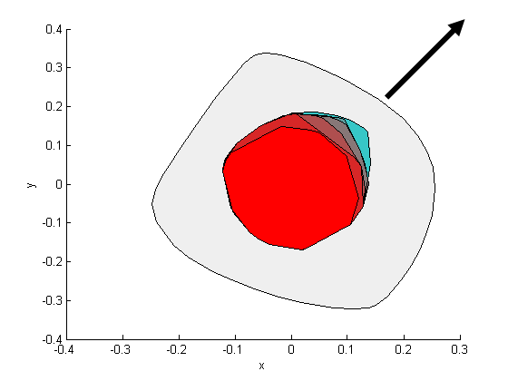
(a) LP starting with DSOS and adding 5 atoms.

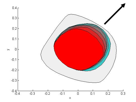
(b) SOCP starting with SDSOS and adding 5 atoms.

Figure 2.1: LP and SOCP-based column generation for inner approximation of a spectrahedron.

Figure 2.1 shows an example of both the LP and SOCP column generation procedures. We produced two $10\times 10$ random symmetric matrices $E$ and $F$. The outer most set is the feasible set of an SDP with the constraint $I+xE+yF\succeq 0.$ (Here, $I$ is the $10\times 10$ identity matrix.) The SDP wishes to maximize $x+y$ over this set. The innermost set in Figure 2.1(a) is the polyhedral set where $I+xE+yF$ is dd. The innermost set in Figure 2.1(b) is the SOCP-representable set where $I+xE+yF$ is sdd. In both cases, we do 5 iterations of column generation that expand these sets by introducing one new atom at a time. These atoms come from the most negative eigenvector (resp. the two most negative eigenvectors) of the dual optimal solution as explained above. Note that in both cases, we are growing our approximation of the positive semidefinite cone in the direction that we care about (the northeast). This is in contrast to algebraic hierarchies based on “positive multipliers” (see the rDSOS and rSDSOS hierarchies in Definition 3.2.2 for example), which completely ignore the objective function.

2.4 Nonconvex polynomial optimization

In this section, we apply the ideas described in the previous section to sum of squares algorithms for nonconvex polynomial optimization. In particular, we consider the NP-hard problem of minimizing a form (of degree $\geq 4$) on the sphere. Recall that $z(x,d)$ is the vector of all monomials in $n$ variables with degree $d$. Let $p(x)$ be a form with $n$ variables and even degree $2d$, and let $\textup{coef}(p)$ be the vector of its coefficients with the monomial ordering given by $z(x,2d)$. Thus $p(x)$ can be viewed as $\textup{coef}(p)^{T}z(x,2d)$. Let $s(x)\mathrel{\mathop{:}}=(\sum_{i=1}^{n}x_{i}^{2})^{d}$. With this notation, the problem of minimizing a form $p$ on the unit sphere can be written as

$$\underset{\lambda}{\max} \lambda$$ (2.8)

s.t. $$p(x)-\lambda s(x)\geq 0,\forall x\in\mathbb{R}^{n}.$$

With the SOS programming approach, the following SDP is solved to get the largest scalar $\lambda$ and an SOS certificate proving that $p(x)-\lambda s(x)$ is nonnegative:

$$\underset{\lambda,Y}{\max} \lambda$$

s.t. $$p(x)-\lambda s(x)=z^{T}(x,d)Yz(x,d),$$

$$Y\succeq 0.$$

The sum of squares certificate is directly read from an eigenvalue decomposition of the solution $Y$ to the SDP above and has the form

$$p(x)-\lambda s(x)\geq\sum_{i}(z^{T}(x,d)u_{i})^{2},$$

where $Y=\sum_{i}u_{i}u_{i}^{T}$. Since all sos polynomials are nonnegative, the optimal value of the SDP in (2.4) is a lower bound to the optimal value of the optimization problem in (2.8). Unfortunately, before solving the SDP, we do not have access to the vectors $u_{i}$ in the decomposition of the optimal matrix $Y$. However, the fact that such vectors exist hints at how we should go about replacing $P_{n}$ by a polyhedral restriction in (2.4): If the constraint $Y\succeq 0$ is changed to

$${Y=\sum_{u\in\mathcal{U}}\alpha_{u}uu^{T},\alpha_{u}\geq 0},$$ (2.10)

where $\mathcal{U}$ is a finite set, then (2.4) becomes an LP. This is one interpretation of Ahmadi and Majumdar’s work in [9, 7] where they replace $P_{n}$ by $DD_{n}$. Indeed, this is equivalent to taking $\mathcal{U}=\mathcal{U}_{n,2}$ in (2.10), as shown in Theorem 2.3.1. We are interested in extending their results by replacing $P_{n}$ by larger restrictions than $DD_{n}$. A natural candidate for example would be obtained by changing $\mathcal{U}_{n,2}$ to $\mathcal{U}_{n,3}$. However, although $\mathcal{U}_{n,3}$ is finite, it contains a very large set of vectors even for small values of $n$ and $d$. For instance, when $n=30$ and $d=4$, $\mathcal{U}_{n,3}$ has over 66 million elements. Therefore we use column generation ideas to iteratively expand $\mathcal{U}$ in a manageable fashion. To initialize our procedure, we would like to start with good enough atoms to have a feasible LP. The following result guarantees that replacing $Y\succeq 0$ with $Y\in DD_{n}$ always yields an initial feasible LP in the setting that we are interested in.

Theorem 2.4.1.

For any form $p$ of degree $2d$, there exists $\lambda\in\mathbb{R}$ such that $p(x)-\lambda(\sum_{i=1}^{n}x_{i}^{2})^{d}$ is dsos.

Proof.

As before, let $s(x)=(\sum_{i=1}^{n}x_{i}^{2})^{d}$. We observe that the form $s(x)$ is strictly in the interior of $DSOS_{n,2d}$. Indeed, by expanding out the expression we see that we can write $s(x)$ as $z^{T}(x,d)Qz(x,d)$, where $Q$ is a diagonal matrix with all diagonal entries positive. So $Q$ is in the interior of $DD_{{n+d-1\choose d}}$, and hence $s(x)$ is in the interior of $DSOS_{n,2d}$. This implies that for $\alpha>0$ small enough, the form

$$(1-\alpha)s(x)+\alpha p(x)$$

will be dsos. Since $DSOS_{n,2d}$ is a cone, the form

$$\frac{(1-\alpha)}{\alpha}s(x)+p(x)$$

will also be dsos. By taking $\lambda$ to be smaller than or equal to $-\frac{1-\alpha}{\alpha}$, the claim is established. ∎

As $DD_{n}\subseteq SDD_{n}$, the theorem above implies that replacing $Y\succeq 0$ with $Y\in SDD_{n}$ also yields an initial feasible SOCP. Motivated in part by this theorem, we will always start our LP-based iterative process with the restriction that $Y\in DD_{n}$. Let us now explain how we improve on this approximation via column generation.

Suppose we have a set $\mathcal{U}$ of vectors in $\mathbb{R}^{n}$, whose outerproducts form all of the rank-one psd atoms that we want to consider. This set could be finite but very large, or even infinite. For our purposes $\mathcal{U}$ always includes $\mathcal{U}_{n,2}$, as we initialize our algorithm with the dsos relaxation. Let us consider first the case where $\mathcal{U}$ is finite: $\mathcal{U}=\{u_{1},\ldots,u_{t}\}.$ Then the problem that we are interested in solving is

$$\underset{\lambda,\alpha_{j}}{\max} \lambda$$

s.t. $$p(x)-\lambda s(x)=z^{T}(x,d)Yz(x,d),$$

$$Y=\sum_{j=1}^{t}\alpha_{j}u_{j}u_{j}^{T},\ \alpha_{j}\geq 0\textup{ for }j=1,\ldots,t.$$

Suppose $z(x,2d)$ has $m$ monomials and let the $i$th monomial in $p(x)$ have coefficient $b_{i}$, i.e., $\textup{coef}(p)=(b_{1},\ldots,b_{m})^{T}$. Also let $s_{i}$ be the $i$th entry in $\textup{coef}(s(x))$. We rewrite the previous problem as

$$\underset{\lambda,\alpha_{j}}{\max} \lambda$$

s.t. $$A_{i}\cdot Y+\lambda s_{i}=b_{i}\textup{ for }i=1,\ldots,m,$$

$$Y=\sum_{j=1}^{t}\alpha_{j}u_{j}u_{j}^{T},\ \alpha_{j}\geq 0\textup{ for }j=1,\ldots,t.$$

where $A_{i}$ is a matrix that collects entries of $Y$ that contribute to the $i^{th}$ monomial in $z(x,2d)$, when $z^{T}(x,d)Yz(x,d)$ is expanded out. The above is equivalent to

$$\underset{\lambda,\alpha_{j}}{\max} \lambda$$

s.t. $$\sum_{j}\alpha_{j}(A_{i}\cdot{u_{j}u_{j}^{T}})+\lambda s_{i}=b_{i}\ \textup{ for }i=1,\ldots,m,$$

$$\alpha_{j}\geq 0\textup{ for }j=1,\ldots,t.$$

The dual problem is

$$\underset{\mu}{\min} \sum_{i=1}^{m}\mu_{i}b_{i}$$

s.t. $$(\sum_{i=1}^{m}\mu_{i}A_{i})\cdot{u_{j}u_{j}^{T}}\geq 0,\ j=1,\ldots,t,$$

$$\sum_{i=1}^{m}\mu_{i}s_{i}=1.$$

In the column generation framework, suppose we consider only a subset of the primal LP variables corresponding to the matrices ${u_{1}u_{1}^{T}},\ldots,{u_{k}u_{k}^{T}}$ for some $k<t$ (call this the reduced primal problem). Let $(\bar{\alpha}_{1},\ldots,\bar{\alpha}_{k})$ stand for an optimal solution of the reduced primal problem and let $\bar{\mu}=(\bar{\mu}_{1},\ldots,\bar{\mu}_{m})$ stand for an optimal dual solution. If we have

$$(\sum_{i=1}^{m}\bar{\mu}_{i}A_{i})\cdot{u_{j}u_{j}^{T}}\geq 0\textup{ for }j=k+1,\ldots,t,$$ (2.12)

then $\bar{\mu}$ is an optimal dual solution for the original larger primal problem with columns $1,\ldots,t$. In other words, if we simply set $\alpha_{k+1}=\cdots=\alpha_{t}=0$, then the solution of the reduced primal problem becomes a solution of the original primal problem. On the other hand, if (2.12) is not true, then suppose the condition is violated for some ${u_{l}u_{l}^{T}}$. We can augment the reduced primal problem by adding the variable $\alpha_{l}$, and repeat this process.

Let $B=\sum_{i=1}^{m}\bar{\mu}_{i}A_{i}$. We can test if (2.12) is false by solving the pricing subproblem:

$$\min_{u\in\mathcal{U}}u^{T}Bu.$$ (2.13)

If $u^{T}Bu<0$, then there is an element $u$ in $\mathcal{U}$ such that the matrix $uu^{T}$ violates the dual constraint written in (2.12). Problem (2.13) may or may not be easy to solve depending on the set $\mathcal{U}.$ For example, an ambitious column generation strategy to improve on dsos (i.e., $\mathcal{U}=\mathcal{U}_{n,2}$), would be to take $\mathcal{U}=\mathcal{U}_{n,n}$; i.e., the set all vectors in $\mathbb{R}^{n}$ consisting of zeros, ones, and minus ones. In this case, the pricing problem (2.13) becomes

$$\min_{u\in\{0,\pm 1\}^{n}}u^{T}Bu.$$

Unfortunately, the above problem generalizes the quadratic unconstrained boolean optimization problem (QUBO) and is NP-hard. Nevertheless, there are good heuristics for this problem (see e.g., [34],[52]) that can be used to find near optimal solutions very fast. While we did not pursue this pricing subproblem, we did consider optimizing over $\mathcal{U}_{n,3}$. We refer to the vectors in $\mathcal{U}_{n,3}$ as “triples” for obvious reasons and generally refer to the process of adding atoms drawn from $U_{n,3}$ as optimizing over “triples”.

Even though one can theoretically solve (2.13) with $\mathcal{U}=\mathcal{U}_{n,3}$ in polynomial time by simple enumeration of $n^{3}$ elements, this is very impractical. Our simple implementation is a partial enumeration and is implemented as follows. We iterate through the triples (in a fixed order), and test to see whether the condition $u^{T}Bu\geq 0$ is violated by a given triple $u$, and collect such violating triples in a list. We terminate the iteration when we collect a fixed number of violating triples (say $t_{1}$). We then sort the violating triples by increasing values of $u^{T}Bu$ (remember, these values are all negative for the violating triples) and select the $t_{2}$ most violated triples (or fewer if less than $t_{2}$ are violated overall) and add them to our current set of atoms. In a subsequent iteration we start off enumerating triples right after the last triple enumerated in the current iteration so that we do not repeatedly scan only the same subset of triples. Although our implementation is somewhat straightforward and can be obviously improved, we are able to demonstrate that optimizing over triples improves over the best bounds obtained by Ahmadi and Majumdar in a similar amount of time (see Section 2.4.2).

We can also have pricing subproblems where the set $\mathcal{U}$ is infinite. Consider e.g. the case $\mathcal{U}=\mathbb{R}^{n}$ in (2.13). In this case, if there is a feasible solution with a negative objective value, then the problem is clearly unbounded below. Hence, we look for a solution with the smallest value of “violation” of the dual constraint divided by the norm of the violating matrix. In other words, we want the expression $u^{T}Bu/\textup{norm}(uu^{T})$ to be as small as possible, where norm is the Euclidean norm of the vector consisting of all entries of $uu^{T}$. This is the same as minimizing $u^{T}Bu/||u||^{2}$. The eigenvector corresponding to the smallest eigenvalue yields such a minimizing solution. This is the motivation behind the strategy described in the previous section for our LP column generation scheme. In this case, we can use a similar strategy for our SOCP column generation scheme. We replace $Y\succeq 0$ by $Y\in SDD_{n}$ in (2.4) and iteratively expand $SDD_{n}$ by using the “two most negative eigenvector technique” described in Section 2.3.2.

2.4.1 Experiments with a 10-variable quartic

We illustrate the behaviour of these different strategies on an example. Let $p(x)$ be a degree-four form defined on 10 variables, where the components of $\textup{coef}(p)$ are drawn independently at random from the normal distribution $\mathcal{N}(0,1)$. Thus $d=2$ and $n=10$, and the form $p(x)$ is ‘fully dense’ in the sense that $\textup{coef}(p)$ has essentially all nonzero components. In Figure 2.2, we show how the lower bound on the optimal value of $p(x)$ over the unit sphere changes per iteration for different methods. The $x$-axis shows the number of iterations of the column generation algorithm, i.e., the number of times columns are added and the LP (or SOCP) is resolved. The $y$-axis shows the lower bound obtained from each LP or SOCP. Each curve represents one way of adding columns. The three horizontal lines (from top to bottom) represent, respectively, the SDP bound, the 1SDSOS bound and the 1DSOS bound. The curve DSOS_k gives the bound obtained by solving LPs, where the first LP has $Y\in DD_{n}$ and subsequent columns are generated from a single eigenvector corresponding to the most negative eigenvalue of the dual optimal solution as described in Section 2.3.1. The LP triples curve also corresponds to an LP sequence, but this time the columns that are added are taken from $U_{n,3}$ and are more than one in each iteration (see the next subsection). This bound saturates when constraints coming from all elements of $U_{n,3}$ are satisfied. Finally, the curve SDSOS_k gives the bound obtained by SOCP-based column generation as explained just above.

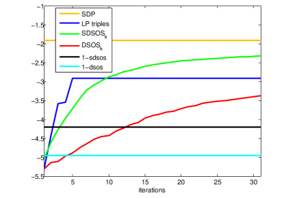
Figure 2.2: Lower bounds for a polynomial of degree 4 in 10 variables obtained via LP and SOCP based column generation

2.4.2 Larger computational experiments

In this section, we consider larger problem instances ranging from 15 variables to 40 variables: these instances are again fully dense and generated in exactly the same way as the $n=10$ example of the previous subsection. However, contrary to the previous subsection, we only apply our “triples” column generation strategy here. This is because the eigenvector-based column generation strategy is too computationally expensive for these problems as we discuss below.

To solve the triples pricing subproblem with our partial enumeration strategy, we set $t_{1}$ to 300,000 and $t_{2}$ to 5000. Thus in each iteration, we find up to 300,000 violated triples, and add up to 5000 of them. In other words, we augment our LP by up to 5000 columns in each iteration. This is somewhat unusual as in practice at most a few dozen columns are added in each iteration. The logic for this is that primal simplex is very fast in reoptimizing an LP when a small number of additional columns are added to an LP whose optimal basis is known. However, in our context, we observed that the associated LPs are very hard for the simplex routines inside our LP solver (CPLEX 12.4) and take much more time than CPLEX’s interior point solver. We therefore use CPLEX’s interior point (“barrier”) solver not only for the initial LP but for subsequent LPs after adding columns. Because interior point solvers do not benefit significantly from warm starts, each LP takes a similar amount of time to solve as the initial LP, and therefore it makes sense to add a large number of columns in each iteration to amortize the time for each expensive solve over many columns.

Table 2.1 is taken from the work of Ahmadi and Majumdar [9], where they report lower bounds on the minimum value of fourth-degree forms on the unit sphere obtained using different methods, and the respective computing times (in seconds).

	n=15		n=20		n=25		n=30		n=40
	bd	t(s)	bd	t(s)	bd	t(s)	bd	t(s)	bd	t(s)
DSOS	-10.96	0.38	-18.012	0.74	-26.45	15.51	-36.85	7.88	-62.30	10.68
SDSOS	-10.43	0.53	-17.33	1.06	-25.79	8.72	-36.04	5.65	-61.25	18.66
1DSOS	-9.22	6.26	-15.72	37.98	-23.58	369.08	NA	NA	NA	NA
1SDSOS	-8.97	14.39	-15.29	82.30	-23.14	538.54	NA	NA	NA	NA
SOS	-3.26	5.60	-3.58	82.22	-3.71	1068.66	NA	NA	NA	NA

Table 2.1: Comparison of optimal values in [9] for lower bounding a quartic form on the sphere for varying dimension, along with run times (in seconds). These results are obtained on a 3.4 GHz Windows computer with 16 GB of memory.

In Table 2.2, we give our bounds for the same problem instances. We report two bounds, obtained at two different times (if applicable). In the first case ( rows labeled R1), the time taken by 1SDSOS in Table 2.1 is taken as a limit, and we report the bound from the last column generation iteration occuring before this time limit; the 1SDSOS bound is the best non-SDP bound reported in the experiments of Ahmadi and Majumdar. In the rows labeled as R2, we take 600 seconds as a limit and report the last bound obtained before this limit. In a couple of instances ($n=15$ and $n=20$), our column generation algorithm terminates before the 600 second limit, and we report the termination time in this case.

	n=15		n=20		n=25		n=30		n=40
	bd	t(s)	bd	t(s)	bd	t(s)	bd	t(s)	bd	t(s)
R1	-6.20	10.96	-12.38	70.70	-20.08	508.63	N/A	N/A	N/A	N/A
R2	-5.57	31.19	-9.02	471.39	-20.08	600	-32.28	600	-35.14	600

Table 2.2: Lower bounds on the optimal value of a form on the sphere for varying degrees of polynomials using Triples on a 2.33 GHz Linux machine with 32 GB of memory.

We observe that in the same amount of time (and even on a slightly slower machine), we are able to consistently beat the 1SDSOS bound, which is the strongest non-SDP bound produced in [9]. We also experimented with the eigenvalue pricing subproblem in the LP case, with a time limit of 600 seconds. For $n=25$, we obtain a bound of $-23.46$ after adding only $33$ columns in 600 seconds. For $n=40$, we are only able to add 6 columns and the lower bound obtained is $-61.49$. Note that this bound is worse than the triples bound given in Table 2.2. The main reason for being able to add so few columns in the time limit is that each column is almost fully dense (the LPs for n=25 have 20,475 rows, and 123,410 rows for $n=40$). Thus, the LPs obtained are very hard to solve after a few iterations and become harder with increasing $n$. As a consequence, we did not experiment with the eigenvalue pricing subproblem in the SOCP case as it is likely to be even more computationally intensive.

2.5 Inner approximations of copositive programs and the maximum stable set problem

Semidefinite programming has been used extensively for approximation of NP-hard combinatorial optimization problems. One such example is finding the stability number of a graph. A stable set (or independent set) of a graph $G=(V,E)$ is a set of nodes of $G$, no two of which are adjacent. The size of the largest stable set of a graph $G$ is called the stability number (or independent set number) of $G$ and is denoted by $\alpha(G).$ Throughout, $G$ is taken to be an undirected, unweighted graph on $n$ nodes. It is known that the problem of testing if $\alpha(G)$ is greater than a given integer $k$ is NP-hard [102]. Furthermore, the stability number cannot be approximated to a factor of $n^{1-\epsilon}$ for any $\epsilon>0$ unless P$=$NP [86]. The natural integer programming formulation of this problem is given by

$$\alpha(G)= \underset{x_{i}}{\max}\sum_{i=1}^{n}x_{i}$$ (2.14)

$$\text{s.t. }x_{i}+x_{j}\leq 1,\forall(i,j)\in E,$$

$$x_{i}\in\{0,1\},\forall i=1,\ldots,n.$$

Although this optimization problem is intractable, there are several computationally-tractable relaxations that provide upper bounds on the stability number of a graph. For example, the obvious LP relaxation of (2.14) can be obtained by relaxing the constraint $x_{i}\in\{0,1\}$ to $x_{i}\in[0,1]$:

$$LP(G)= \underset{x_{i}}{\max}\sum_{i}x_{i}$$ (2.15)

$$\text{s.t. }x_{i}+x_{j}\leq 1,\forall(i,j)\in E,$$

$$x_{i}\in[0,1],\forall i=1,\ldots,n.$$

This bound can be improved upon by adding the so-called clique inequalities to the LP, which are of the form $x_{i_{1}}+x_{i_{2}}+\ldots+x_{i_{k}}\leq 1$ when nodes $(i_{1},i_{2},\ldots,i_{k})$ form a clique in $G$. Let $C_{k}$ be the set of all $k$-clique inequalities in $G$. This leads to a hierarchy of LP relaxations:

$$LP_{k}(G)= \max\sum_{i}x_{i},$$ (2.16)

$$x_{i}\in[0,1],\forall i=1,\ldots,n,$$

$$C_{2},\ldots,C_{k}\text{ are satisfied.}$$

Notice that for $k=2,$ this simply corresponds to (2.15), in other words, $LP_{2}(G)=LP(G)$.

In addition to LPs, there are also semidefinite programming (SDP) relaxations that provide upper bounds to the stability number. The most well-known is perhaps the Lovász theta number $\vartheta(G)$ [128], which is defined as the optimal value of the following SDP:

$$\vartheta(G)\mathrel{\mathop{:}}= \underset{X}{\max}~{}J\cdot X$$ (2.17)

$$\text{s.t. }I\cdot X=1,$$

$$X_{i,j}=0,\forall(i,j)\in E$$

$$X\in P_{n}.$$

Here $J$ is the all-ones matrix and $I$ is the identity matrix of size $n$. The Lovász theta number is known to always give at least as good of an upper bound as the LP in (2.15), even with the addition of clique inequalities of all sizes (there are exponentially many); see, e.g., [116, Section 6.5.2] for a proof. In other words,

$$\vartheta(G)\leq LP_{k}(G),\forall k.$$

An alternative SDP relaxation for stable set is due to de Klerk and Pasechnik. In [55], they show that the stability number can be obtained through a conic linear program over the set of copositive matrices. Namely,

$$\alpha(G)= \min_{\lambda}\lambda$$ (2.18)

$$\text{s.t. }\lambda(I+A)-J\in C_{n},$$

where $A$ is the adjacency matrix of $G$. Replacing $C_{n}$ by the restriction $P_{n}+N_{n}$, one obtains the aforementioned relaxation through the following SDP

$$SDP(G)\mathrel{\mathop{:}}= \min_{\lambda,X}\lambda$$ (2.19)

$$\text{s.t. }\lambda(I+A)-J\geq X,$$

$$X\in P_{n}.$$

This latter SDP is more expensive to solve than the Lovász SDP (2.17), but the bound that it obtains is always at least as good (and sometimes strictly better). A proof of this statement is given in [55, Lemma 5.2], where it is shown that (2.19) is an equivalent formulation of an SDP of Schrijver [174], which produces stronger upper bounds than (2.17).

Another reason for the interest in the copositive approach is that it allows for well-known SDP and LP hierarchies—developed respectively by Parrilo [152, Section 5] and de Klerk and Pasechnik [55]—that produce a sequence of improving bounds on the stability number. In fact, by appealing to Positivstellensatz results of Pólya [158], and Powers and Reznick [160], de Klerk and Pasechnik show that their LP hierarchy produces the exact stability number in $\alpha^{2}(G)$ number of steps [55, Theorem 4.1]. This immediately implies the same result for stronger hierarchies, such as the SDP hierarchy of Parrilo [152], or the rDSOS and rSDSOS hierarchies of Ahmadi and Majumdar [9].

One notable difficulty with the use of copositivity-based SDP relaxations such as (2.19) in applications is scalibility. For example, it takes more than 5 hours to solve (2.19) when the input is a randomly generated Erdós-Renyi graph with 300 nodes and edge probability $p=0.8$. Hence, instead of using (2.19), we will solve a sequence of LPs/SOCPs generated in an iterative fashion. These easier optimization problems will provide upper bounds on the stability number in a more reasonable amount of time, though they will be weaker than the ones obtained via (2.19).

We will derive both our LP and SOCP sequences from formulation (2.18) of the stability number. To obtain the first LP in the sequence, we replace $C_{n}$ by $DD_{n}+N_{n}$ (instead of replacing $C_{n}$ by $P_{n}+N_{n}$ as was done in (2.19)) and get

$$DSOS_{1}(G)\mathrel{\mathop{:}}= \min_{\lambda,X}\lambda$$ (2.20)

$$\text{s.t. }\lambda(I+A)-J\geq X,$$

$$X\in DD_{n}.$$

This is an LP whose optimal value is a valid upper bound on the stability number as $DD_{n}\subseteq P_{n}$.

Theorem 2.5.1.

The LP in (2.20) is always feasible.

Proof.

We need to show that for any $n\times n$ adjacency matrix $A$, there exists a diagonally dominant matrix $D$, a nonnegative matrix $N$, and a scalar $\lambda$ such that

$$\lambda(I+A)-J=D+N.$$ (2.21)

Notice first that $\lambda(I+A)-J$ is a matrix with $\lambda-1$ on the diagonal and at entry $(i,j)$, if $(i,j)$ is an edge in the graph, and with $-1$ at entry $(i,j)$ if $(i,j)$ is not an edge in the graph. If we denote by $d_{i}$ the degree of node $i$, then let us take $\lambda=n-\min_{i}d_{i}+1$ and $D$ a matrix with diagonal entries $\lambda-1$ and off-diagonal entries equal to $0$ if there is an edge, and $-1$ if not. This matrix is diagonally dominant as there are at most $n-\min_{i}d_{i}$ minus ones on each row. Furthermore, if we take $N$ to be a matrix with $\lambda-1$ at the entries $(i,j)$ where $(i,j)$ is an edge in the graph, then (2.21) is satisfied and $N\geq 0$. ∎

Feasibility of this LP is important for us as it allows us to initiate column generation. By contrast, if we were to replace the diagonal dominance constraint by a diagonal constraint for example, the LP could fail to be feasible. This fact has been observed by de Klerk and Pasechnik in [55] and Bomze and de Klerk in [32].

To generate the next LP in the sequence via column generation, we think of the extreme-ray description of the set of diagonally dominant matrices as explained in Section 2.3. Theorem 2.3.1 tells us that these are given by the matrices in $U_{n,2}$ and so we can rewrite (2.20) as

$$DSOS_{1}(G)\mathrel{\mathop{:}}= \min_{\lambda,\alpha_{i}}\lambda$$ (2.22)

$$\text{s.t. }\lambda(I+A)-J\geq X,$$

$$X=\sum_{u_{i}u_{i}^{T}\in{U}_{n,2}}\alpha_{i}u_{i}u_{i}^{T},$$

$$\alpha_{i}\geq 0,\ i=1,\ldots,n^{2}.$$

The column generation procedure aims to add new matrix atoms to the existing set $U_{n,2}$ in such a way that the current bound $DSOS_{1}$ improves. There are numerous ways of choosing these atoms. We focus first on the cutting plane approach based on eigenvectors. The dual of (2.22) is the LP

$$DSOS_{1}(G)\mathrel{\mathop{:}}= \max_{X}J\cdot X,$$ (2.23)

$$\text{s.t. }(A+I)\cdot X=1,$$

$$X\geq 0,$$

$$(u_{i}u_{i}^{T})\cdot X\geq 0,\forall u_{i}u_{i}^{T}\in{U}_{n,2}.$$

If our optimal solution $X^{*}$ to (2.23) is positive semidefinite, then we are obtaining the best bound we can possibly produce, which is the SDP bound of (2.19). If this is not the case however, we pick our atom matrix to be the outer product $uu^{T}$ of the eigenvector $u$ corresponding to the most negative eigenvalue of $X^{*}$. The optimal value of the LP

$$DSOS_{2}(G)\mathrel{\mathop{:}}= \max_{X}J\cdot X,$$ (2.24)

$$\text{s.t. }(A+I)\cdot X=1,$$

$$X\geq 0,$$

$$(u_{i}u_{i}^{T})\cdot X\geq 0,\forall u_{i}u_{i}^{T}\in{U}_{n,2},$$

$$(uu^{T})\cdot X\geq 0$$

that we derive is guaranteed to be no worse than $DSOS_{1}$ as the feasible set of (2.24) is smaller than the feasible set of (2.23). Under mild nondegeneracy assumptions (satisfied, e.g., by uniqueness of the optimal solution to (2.23)), the new bound will be strictly better. By reiterating the same process, we create a sequence of LPs whose optimal values $DSOS_{1},DSOS_{2},\ldots$ are a nonincreasing sequence of upper bounds on the stability number.

Generating the sequence of SOCPs is done in an analogous way. Instead of replacing the constraint $X\in P_{n}$ in (2.19) by $X\in DD_{n}$, we replace it by $X\in SDD_{n}$ and get

$$SDSOS_{1}(G)\mathrel{\mathop{:}}= \min_{\lambda,X}\lambda$$ (2.25)

$$\text{s.t. }\lambda(I+A)-J\geq X,$$

$$X\in SDD_{n}.$$

Once again, we need to reformulate the problem in such a way that the set of scaled diagonally dominant matrices is described as some combination of psd “atom” matrices. In this case, we can write any matrix $X\in SDD_{n}$ as

$$X=\sum_{V_{i}\in\mathcal{V}_{n,2}}V_{i}\begin{pmatrix}a_{i}^{1}&a_{i}^{2}\\ a_{i}^{2}&a_{i}^{3}\end{pmatrix}V_{i}^{T},$$

where $a_{i}^{1},a_{i}^{2},a_{i}^{3}$ are variables making the $2\times 2$ matrix psd, and the $V_{i}$’s are our atoms. Recall from Section 2.3 that the set $\mathcal{V}_{n,2}$ consists of all $n\times 2$ matrices which have zeros everywhere, except for a 1 in the first column in position $j$ and a 1 in the second column in position $k\neq j$. This gives rise to an equivalent formulation of (2.25):

$$SDSOS_{1}(G)\mathrel{\mathop{:}}= \min_{\lambda,a_{i}^{j}}\lambda$$ (2.26)

$$\text{s.t. }\lambda(I+A)-J\geq X$$

$$X=\sum_{V_{i}\in\mathcal{V}_{n,2}}V_{i}\begin{pmatrix}a_{i}^{1}&a_{i}^{2}\\ a_{i}^{2}&a_{i}^{3}\end{pmatrix}V_{i}^{T}$$

$$\begin{pmatrix}a_{i}^{1}&a_{i}^{2}\\ a_{i}^{2}&a_{i}^{3}\end{pmatrix}\succeq 0,\ i=1,\ldots,\binom{n}{2}.$$

Just like the LP case, we now want to generate one (or more) $n\times 2$ matrix $V$ to add to the set $\{V_{i}\}_{i}$ so that the bound $SDSOS_{1}$ improves. We do this again by using a cutting plane approach originating from the dual of (2.26):

$$SDSOS_{1}(G)\mathrel{\mathop{:}}= \max_{X}J\cdot X$$ (2.27)

$$\text{s.t. }(A+I)\cdot X=1,$$

$$X\geq 0,$$

$$V_{i}^{T}\cdot XV_{i}\succeq 0,\ i=1,\ldots,\binom{n}{2}.$$

Note that strong duality holds between this primal-dual pair as it is easy to check that both problems are strictly feasible. We then take our new atom to be

$$V=(w_{1}~{}w_{2}),$$

where $w_{1}$ and $w_{2}$ are two eigenvectors corresponding to the two most negative eigenvalues of $X^{*}$, the optimal solution of (2.27). If $X^{*}$ only has one negative eigenvalue, we add a linear constraint to our problem; if $X^{*}\succeq 0$, then the bound obtained is identical to the one obtained through SDP (2.19) and we cannot hope to improve. Our next iterate is therefore

$$SDSOS_{2}(G)\mathrel{\mathop{:}}= \max_{X}J\cdot X$$ (2.28)

$$\text{s.t. }(A+I)\cdot X=1,$$

$$X\geq 0,$$

$$V_{i}^{T}\cdot XV_{i}\succeq 0,\ i=1,\ldots,\binom{n}{2},$$

$$V^{T}\cdot XV\succeq 0.$$

Note that the optimization problems generated iteratively in this fashion always remain SOCPs and their optimal values form a nonincreasing sequence of upper bounds on the stability number.

To illustrate the column generation method for both LPs and SOCPs, we consider the complement of the Petersen graph as shown in Figure 2.3(a) as an example. The stability number of this graph is 2 and one of its maximum stable sets is designated by the two white nodes. In Figure 2.3(b), we compare the upper bound obtained via (2.19) and the bounds obtained using the iterative LPs and SOCPs as described in (2.24) and (2.28).

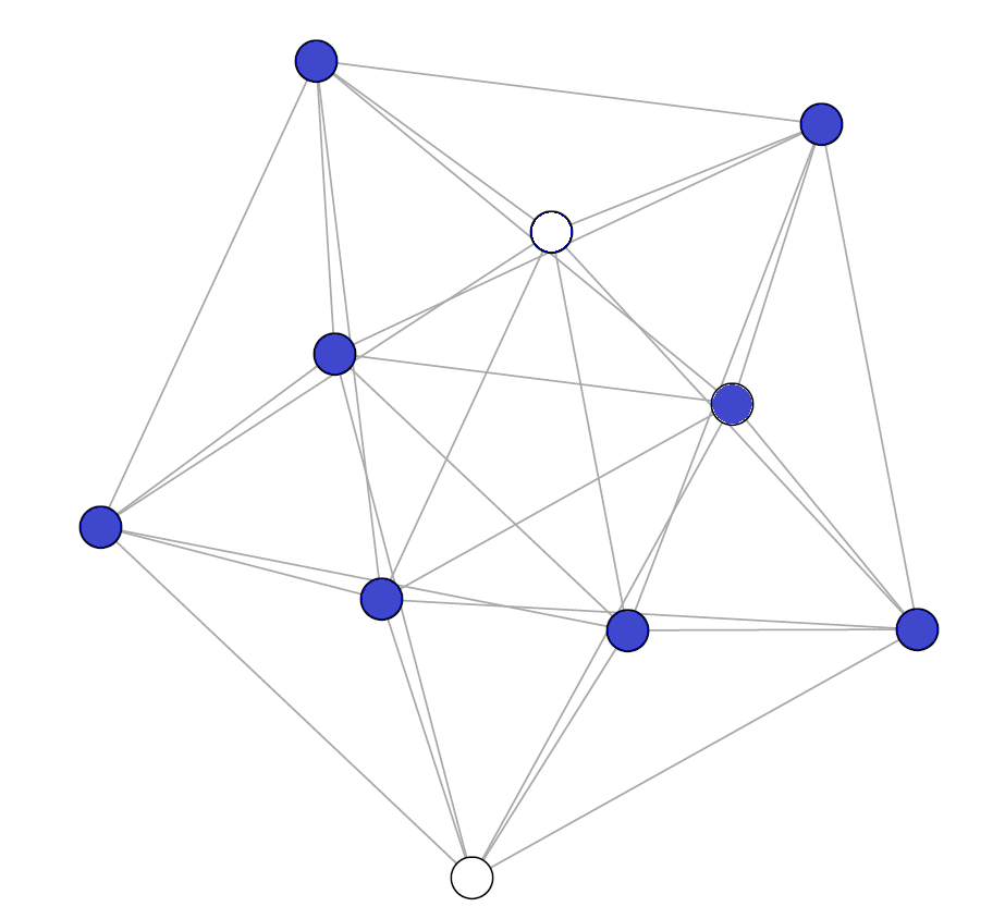
(a) The complement of Petersen Graph

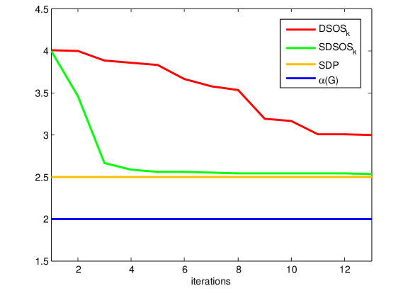
(b) Upper bounds on the stable set number $\alpha(G)$

Figure 2.3: Bounds obtained through SDP (2.19) and iterative SOCPs and LPs for the complement of the Petersen graph.

Note that it takes 3 iterations for the SOCP sequence to produce an upper bound strictly within one unit of the actual stable set number (which would immediately tell us the value of $\alpha$), whereas it takes 13 iterations for the LP sequence to do the same. It is also interesting to compare the sequence of LPs/SOCPs obtained through column generation to the sequence that one could obtain using the concept of $r$-dsos/$r$-sdsos polynomials. Indeed, LP (2.20) (resp. SOCP (2.25)) can be written in polynomial form as

$$DSOS_{1}(G)\text{ (resp. $SDSOS_{1}(G)$)}= \min_{\lambda}\lambda$$ (2.29)

$$\text{s.t. }\begin{pmatrix}x_{1}^{2}\\ \vdots\\ x_{n}^{2}\end{pmatrix}^{T}(\lambda(I+A)-J)\begin{pmatrix}x_{1}^{2}\\ \vdots\\ x_{n}^{2}\end{pmatrix}\text{ is dsos (resp. sdsos).}$$

Iteration $k$ in the sequence of LPs/SOCPs would then correspond to requiring that this polynomial be $k$-dsos or $k$-sdsos. For this particular example, we give the 1-dsos, 2-dsos, 1-sdsos and 2-sdsos bounds in Table 2.3.

Iteration	$r$-dsos bounds	$r$-sdsos bounds
$r=0$	4.00	4.00
$r=1$	2.71	2.52
$r=2$	2.50	2.50

Table 2.3: Bounds obtained through rDSOS and rSDSOS hierarchies.

Though this sequence of LPs/SOCPs gives strong upper bounds, each iteration is more expensive than the iterations done in the column generation approach. Indeed, in each of the column generation iterations, only one constraint is added to our problem, whereas in the rDSOS/rSDSOS hierarchies, the number of constraints is roughly multiplied by $n^{2}$ at each iteration.

Finally, we investigate how these techniques perform on graphs with a large number of nodes, where the SDP bound cannot be found in a reasonable amount of time. The graphs we test these techniques on are Erdös-Rényi graphs $ER(n,p)$; i.e. graphs on $n$ nodes where an edge is added between each pair of nodes independently and with probability $p$. In our case, we take $n$ to be between $150$ and $300$, and $p$ to be either $0.3$ or $0.8$ so as to experiment with both medium and high density graphs.

In Table 2.4, we present the results of the iterative SOCP procedure and contrast them with the SDP bounds. The third column of the table contains the SOCP upper bound obtained through (2.27); the solver time needed to obtain this bound is given in the fourth column. The fifth and sixth columns correspond respectively to the SOCP iterative bounds obtained after 5 mins solving time and 10 mins solving time. Finally, the last two columns chart the SDP bound obtained from (2.19) and the time in seconds needed to solve the SDP. All SOCP and SDP experiments were done using Matlab, the solver MOSEK [140], the SPOTLESS toolbox [137], and a computer with 3.4 GHz speed and 16 GB RAM.

n	p	$SDSOS_{1}$	time (s)	$SDSOS_{k}$ (5 mins)	$SDSOS_{k}$ (10 mins)	$SDP(G)$	time (s)
150	0.3	105.70	1.05	39.93	37.00	20.43	221.13
150	0.8	31.78	1.07	9.96	9.43	6.02	206.28
200	0.3	140.47	1.84	70.15	56.37	23.73	1,086.42
200	0.8	40.92	2.07	12.29	11.60	6.45	896.84
250	0.3	176.25	3.51	111.63	92.93	26.78	4,284.01
250	0.8	51.87	3.90	17.25	15.39	7.18	3,503.79
300	0.3	210.32	5.69	151.71	134.14	29.13	32,300.60
300	0.8	60.97	5.73	19.53	17.24	7.65	20,586.02

Table 2.4: SDP bounds and iterative SOCP bounds obtained on ER(n,p) graphs.

From the table, we note that it is better to run the SDP rather than the SOCPs for small $n$, as the bounds obtained are better and the times taken to do so are comparable. However, as $n$ gets bigger, the SOCPs become valuable as they provide good upper bounds in reasonable amounts of time. For example, for $n=300$ and $p=0.8$, the SOCP obtains a bound that is only twice as big as the SDP bound, but it does so 30 times faster. The sparser graphs don’t do as well, a trend that we will also observe in Table 2.5. Finally, notice that the improvement in the first 5 mins is significantly better than the improvement in the last 5 mins. This is partly due to the fact that the SOCPs generated at the beginning are sparser, and hence faster to solve.

In Table 2.5, we present the results of the iterative LP procedure used on the same instances. All LP results were obtained using a computer with 2.3 GHz speed and 32GB RAM and the solver CPLEX 12.4 [47]. The third and fourth columns in the table contain the LP bound obtained with (2.23) and the solver time taken to do so. Columns 5 and 6 correspond to the LP iterative bounds obtained after 5 mins solving time and 10 mins solving time using the eigenvector-based column generation technique (see discussion around (2.24)). The seventh and eighth columns are the standard LP bounds obtained using (2.16) and the time taken to obtain the bound. Finally, the last column gives bounds obtained by column generation using “triples”, as described in Section 2.4.2. In this case, we take $t_{1}=300,000$ and $t_{2}=500$.

n	p	$DSOS_{1}$	time (s)	$DSOS_{k}$ (5m)	$DSOS_{k}$ (10m)	$LP_{2}$	time (s)	$LP_{triples}$ (10m)
150	0.3	117	$<1$	110.64	110.26	75	$<1$	89.00
150	0.8	46	$<1$	24.65	19.13	75	$<1$	23.64
200	0.3	157	$<1$	147.12	146.71	100	$<1$	129.82
200	0.8	54	$<1$	39.27	36.01	100	$<1$	30.43
250	0.3	194	$<1$	184.89	184.31	125	$<1$	168.00
250	0.8	68	$<1$	55.01	53.18	125	$<1$	40.19
300	0.3	230	$<1$	222.43	221.56	150	$<1$	205.00
300	0.8	78	$<1$	65.77	64.84	150	$<1$	60.00

Table 2.5: LP bounds obtained on the same $ER(n,p)$ graphs.

We note that in this case the upper bound with triples via column generation does better for this range of $n$ than eigenvector-based column generation in the same amount of time. Furthermore, the iterative LP scheme seems to perform better in the dense regime. In particular, the first iteration does significantly better than the standard LP for $p=0.8$, even though both LPs are of similar size. This would remain true even if the 3-clique inequalities were added as in (2.16), since the optimal value of $LP_{3}$ is always at least $n/3$. This is because the vector $(\frac{1}{3},\ldots,\frac{1}{3})$ is feasible to the LP in (2.16) with $k=3$. Note that this LP would have order $n^{3}$ constraints, which is more expensive than our LP. On the contrary, for sparse regimes, the standard LP, which hardly takes any time to solve, gives better bounds than ours.

Overall, the high-level conclusion is that running the SDP is worthwhile for small sizes of the graph. As the number of nodes increases, column generation becomes valuable, providing upper bounds in a reasonable amount of time. Contrasting Tables 2.4 and 2.5, our initial experiments seem to show that the iterative SOCP bounds are better than the ones obtained using the iterative LPs. It may be valuable to experiment with different approaches to column generation however, as the technique used to generate the new atoms seems to impact the bounds obtained.

2.6 Conclusions and future research

For many problems of discrete and polynomial optimization, there are hierarchies of SDP-based sum of squares algorithms that produce provably optimal bounds in the limit [153], [109]. However, these hierarchies can often be expensive computationally. In this chapter, we were interested in problem sizes where even the first level of the hierarchy is too expensive, and hence we resorted to algorithms that replace the underlying SDPs with LPs or SOCPs. We built on the recent work of Ahmadi and Majumdar on DSOS and SDSOS optimization [9], [7], which serves exactly this purpose. We showed that by using ideas from linear programming column generation, the performance of their algorithms is improvable. We did this by iteratively optimizing over increasingly larger structured subsets of the cone of positive semidefinite matrices, without resorting to the more expensive rDSOS and rSDSOS hierarchies.

There is certainly a lot of room to improve our column generation algorithms. In particular, we only experimented with a few types of pricing subproblems and particular strategies for solving them. The success of column generation often comes from good “engineering”, which fine-tunes the algorithms to the problem at hand. Developing warm-start strategies for our iterative SOCPs for example, would be a very useful problem to work on in the future.

Here is another interesting research direction, which for illustrative purposes we outline for the problem studied in Section 2.4; i.e., minimizing a form on the sphere. Recall that given a form $p$ of degree $2d$, we are trying to find the largest $\lambda$ such that $p(x)-\lambda(\sum_{i=1}^{n}x_{i}^{2})^{d}$ is a sum of squares. Instead of solving this sum of squares program, we looked for the largest $\lambda$ for which we could write $p(x)-\lambda$ as a conic combination of a certain set of nonnegative polynomials. These polynomials for us were always either a single square or a sum of squares of polynomials. There are polynomials, however, that are nonnegative but not representable as a sum of squares. Two classic examples [141], [44] are the Motzkin polynomial

$$M(x,y,z)=x^{6}+y^{4}z^{2}+y^{2}z^{4}-3x^{2}y^{2}z^{2},$$

and the Choi-Lam polynomial

$$CL(w,x,y,z)=w^{4}+x^{2}y^{2}+y^{2}z^{2}+x^{2}z^{2}-4wxyz.$$

Either of these polynomials can be shown to be nonnegative using the arithmetic mean-geometric mean (am-gm) inequality, which states that if $x_{1},\ldots,x_{k}\in\mathbb{R}$, then

$$x_{1},\ldots,x_{k}\geq 0\Rightarrow(\sum_{i=1}^{k}x_{i})/k\geq(\Pi_{i=1}^{k}x_{i})^{\frac{1}{k}}.$$

For example, in the case of the Motzkin polynomial, it is clear that the monomials $x^{6},y^{4}z^{2}$ and $y^{2}z^{4}$ are nonnegative for all $x,y,z\in\mathbb{R}$, and letting $x_{1},x_{2},x_{3}$ stand for these monomials respectively, the am-gm inequality implies that

$$x^{6}+y^{4}z^{2}+y^{2}z^{4}\geq 3x^{2}y^{2}z^{2}\mbox{ for all }x,y,z\in\mathbb{R}.$$

These polynomials are known to be extreme in the cone of nonnegative polynomials and they cannot be written as a sum of squares (sos) [165].

It would be interesting to study the separation problems associated with using such non-sos polynomials in column generation. We briefly present one separation algorithm for a family of polynomials whose nonnegativity is provable through the am-gm inequality and includes the Motzkin and Choi-Lam polynomials. This will be a relatively easy-to-solve integer program in itself, whose goal is to find a polynomial $q$ amongst this family which is to be added as our new “nonnegative atom”.

The family of $n$-variate polynomials under consideration consists of polynomials with only $k+1$ nonzero coefficients, with $k$ of them equal to one, and one equal to $-k$. (Notice that the Motzkin and the Choi-Lam polynomials are of this form with $k$ equal to three and four respectively.) Let $m$ be the number of monomials in $p$. Given a dual vector $\mu$ of (2.4) of dimension $m$, one can check if there exists a nonnegative degree $2d$ polynomial $q(x)$ in our family such that $\mu\cdot\textup{coef}(q(x))<0.$ This can be done by solving the following integer program (we assume that $p(x)=\sum_{i=1}^{m}x^{\alpha_{i}}$):

$$\underset{c,y}{\min} \sum_{i=1}^{m}\mu_{i}c_{i}-\sum_{i=1}^{m}k\mu_{i}y_{i}$$ (2.30)

s.t. $$\sum_{i:\alpha_{i}\mbox{ is even}}\alpha_{i}c_{i}=k\sum_{i=1}^{m}\alpha_{i}y_{i},$$

$$\sum_{i=1}^{m}c_{i}=k,$$

$$\sum_{i=1}^{m}y_{i}=1,$$

$$c_{i}\in\{0,1\},y_{i}\in\{0,1\},i=1,\ldots,m,c_{i}=0\mbox{ if }\alpha_{i}\mbox{ is not even.}$$

Here, we have $\alpha_{i}\in\mathbb{N}^{n}$ and the variables $c_{i},y_{i}$ form the coefficients of the polynomial $q(x)=\sum_{i=1}^{m}c_{i}x^{\alpha_{i}}-k\sum_{i=1}^{m}y_{i}x^{\alpha_{i}}$. The above integer program has $2m$ variables, but only $n+2$ constraints (not counting the integer constraints). If a polynomial $q(x)$ with a negative objective value is found, then one can add it as a new atom for column generation. In our specific randomly generated polynomial optimization examples, such polynomials did not seem to help in our preliminary experiments. Nevertheless, it would be interesting to consider other instances and problem structures.

Similarly, in the column generation approach to obtaining inner approximations of the copositive cone, one need not stick to positive semidefinite matrices. It is known that the $5\times 5$ “Horn matrix” [38] for example is extreme in the copositive cone but cannot be written as the sum of a nonnegative and a positive semidefinite matrix. One could define a separation problem for a family of Horn-like matrices and add them in a column generation approach. Exploring such strategies is left for future research.

Chapter 3 Sum of Squares Basis Pursuit with Linear and Second Order Cone Programming

3.1 Introduction

In recent years, semidefinite programming [192] and sum of squares optimization [153, 109, 145] have proven to be powerful techniques for tackling a diverse set of problems in applied and computational mathematics. The reason for this, at a high level, is that several fundamental problems arising in discrete and polynomial optimization [115, 80, 8] or the theory of dynamical systems [152, 90, 1] can be cast as linear optimization problems over the cone of nonnegative polynomials. This observation puts forward the need for efficient conditions on the coefficients $c_{\alpha}\mathrel{\mathop{:}}=c_{\alpha_{1},\ldots,\alpha_{n}}$ of a multivariate polynomial

$$p(x)=\sum_{\alpha}c_{\alpha_{1},\ldots,\alpha_{n}}x_{1}^{\alpha_{1}}\ldots x_{n}^{\alpha_{n}}$$

that ensure the inequality $p(x)\geq 0,$ for all $x\in\mathbb{R}^{n}$. If $p$ is a quadratic function, $p(x)=x^{T}Qx+2c^{T}x+b,$ then nonnegativity of $p$ is equivalent to the $(n+1)\times(n+1)$ symmetric matrix

$$\begin{pmatrix}Q&c\\ c^{T}&b\end{pmatrix}$$

being positive semidefinite and this constraint can be imposed by semidefinite programming. For higher degrees, however, imposing nonnegativity of polynomials is in general an intractable computational task. In fact, even checking if a given quartic polynomial is nonnegative is NP-hard [59]. A particularly popular and seemingly powerful sufficient condition for a polynomial $p$ to be nonnegative is for it to decompose as a sum of squares of other polynomials:

$$p(x)=\sum_{i}q_{i}^{2}(x).$$

This condition is attractive for several reasons. From a computational perspective, for fixed-degree polynomials, a sum of squares decomposition can be checked (or imposed as a constraint) by solving a semidefinite program of size polynomial in the number of variables. From a representational perspective, such a decomposition certifies nonnegativity of $p$ in terms of an easily verifiable algebraic identity. From a practical perspective, the so-called “sum of squares relaxation” is well-known to produce powerful (often exact) bounds on optimization problems that involve nonnegative polynomials; see, e.g., [155]. The reason for this is that constructing examples of nonnegative polynomials that are not sums of squares in relatively low dimensions and degrees seems to be a difficult task, especially when additional structure arising from applications is required.

We have recently been interested in leveraging the attractive features of semidefinite programs (SDPs) and sum of squares (SOS) programs, while solving much simpler classes of convex optimization problems, namely linear programs (LPs) and second order cone programs (SOCPs). Such a research direction can potentially lead to a better understanding of the relative power of different classes of convex relaxations. It also has obvious practical motivations as simpler convex programs come with algorithms that have better scalability and improved numerical conditioning properties. This chapter is a step in this research direction. We present a scheme for solving a sequence of LPs or SOCPs that provide increasingly accurate approximations to the optimal value and the optimal solution of a semidefinite (or a sum of squares) program. With the algorithms that we propose, one can use one of many mature LP/SOCP solvers such as [47, 79, 140], including simplex-based LP solvers, to obtain reasonable approximations to the optimal values of these more difficult convex optimization problems.

The intuition behind our approach is easy to describe with a contrived example. Suppose we would like to show that the degree-4 polynomial

$$\begin{array}[]{lll}p(x)&=&x_{1}^{4}-6x_{1}^{3}x_{2}+2x_{1}^{3}x_{3}+6x_{1}^{2}x_{3}^{2}+9x_{1}^{2}x_{2}^{2}-6x_{1}^{2}x_{2}x_{3}-14x_{1}x_{2}x_{3}^{2}+4x_{1}x_{3}^{3}\\ &&+5x_{3}^{4}-7x_{2}^{2}x_{3}^{2}+16x_{2}^{4}\end{array}$$

has a sum of squares decomposition. One way to do this is to attempt to write $p$ as

$${p(x)=z^{T}(x)Qz(x),}$$

where

$$z(x)=(x_{1}^{2},x_{1}x_{2},x_{2}^{2},x_{1}x_{3},x_{2}x_{3},x_{3}^{2})^{T}$$ (3.1)

is the standard (homogeneous) monomial basis of degree 2 and the matrix $Q$, often called the Gram matrix, is symmetric and positive semidefinite. The search for such a $Q$ can be done with semidefinite programming; one feasible solution e.g. is as follows:

$$Q=\begin{pmatrix}1&-3&0&1&0&2\\ -3&9&0&-3&0&-6\\ 0&0&16&0&0&-4\\ 1&-3&0&2&-1&2\\ 0&0&0&-1&1&0\\ 2&-6&4&2&0&5\end{pmatrix}.$$

Suppose now that instead of the basis $z$ in (3.1), we pick a different basis

$${\tilde{z}(x)=(2x_{1}^{2}-6x_{1}x_{2}+2x_{1}x_{3}+2x_{3}^{2},\quad x_{1}x_{3}-x_{2}x_{3},\quad x_{2}^{2}-\frac{1}{4}x_{3}^{2})^{T}.}$$ (3.2)

With this new basis, we can get a sum of squares decomposition of $p$ by writing it as

$$p(x)=\tilde{z}^{T}(x)\begin{pmatrix}\frac{1}{2}&0&0\\ 0&1&0\\ 0&0&4.\end{pmatrix}\tilde{z}(x).$$

In effect, by using a better basis, we have simplified the Gram matrix and made it diagonal. When the Gram matrix is diagonal, its positive semidefiniteness can be imposed as a linear constraint (diagonals should be nonnegative).

Of course, the catch here is that we do not have access to the magic basis $\tilde{z}(x)$ in (3.2) a priori. Our goal will hence be to “pursue” this basis (or other good bases) by starting with an arbitrary basis (typically the standard monomial basis), and then iteratively improving it by solving a sequence of LPs or SOCPs and performing some efficient matrix decomposition tasks in the process. Unlike the intentionally simplified example we gave above, we will not ever require our Gram matrices to be diagonal. This requirement is too strong and would frequently lead to our LPs and SOCPs being infeasible. The underlying reason for this is that the cone of diagonal matrices is not full dimensional in the cone of positive semidefinite matrices. Instead, we will be after bases that allow the Gram matrix to be diagonally dominant or scaled diagonally dominant (see Definition 5.3.1). The use of these matrices in polynomial optimization has recently been proposed by Ahmadi and Majumdar [9, 7]. We will be building on and improving upon their results in this chapter.

3.1.1 Organization of this chapter

The organization of the rest of the chapter is as follows. In Section 3.2, we introduce some notation and briefly review the concepts of “dsos and sdsos polynomials” which are used later as the first step of an iterative algorithm that we propose in Section 3.3. In this section, we explain how we inner approximate semidefinite (Subsection 3.3.1) and sum of squares (Subsection 3.3.2) cones with LP and SOCP-based cones by iteratively changing bases. In Subsection 3.3.3, we give a different interpretation of our LPs in terms of their corner description as opposed to their facet description. Subsection 3.3.4 is about duality, which is useful for iteratively outer approximating semidefinite or sum of squares cones.

In Section 3.4, we apply our algorithms to the Lovász semidefinite relaxation of the maximum stable set problem. It is shown numerically that our LPs and SOCPs converge to the SDP optimal value in very few iterations and outperform some other well-known LP relaxations on a family of randomly generated examples. In Section 3.5, we consider the partition problem from discrete optimization. As opposed to the stable set problem, the quality of our relaxations here is rather poor. In fact, even the sum of squares relaxation fails on some completely trivial instances. We show this empirically on random instances, and formally prove it on one representative example (Subsection 3.5.1). The reason for this failure is existence of a certain family of quartic polynomials that are nonnegative but not sums of squares.

3.2 Preliminaries

We denote the set of real symmetric $n\times n$ matrices by $S_{n}$. Given two matrices $A$ and $B$ in $S_{n}$, their standard matrix inner product is denoted by $A\cdot B:=\sum_{i,j}A_{ij}B_{ij}=\mbox{ Trace}(AB)$. A symmetric matrix $A$ is positive semidefinite (psd) if $x^{T}Ax\geq 0$ for all $x\in\mathbb{R}^{n}$; this will be denoted by the standard notation $A\succeq 0$, and our notation for the set of $n\times n$ psd matrices is $P_{n}$. We say that $A$ is positive definite (pd) if $x^{T}Ax>0$ for all $x\neq 0$. Any psd matrix $A$ has an upper triangular Cholesky factor $U=\text{chol}(A)$ satisfying $A=U^{T}U$. When $A$ is pd, the Cholesky factor is unique and has positive diagonal entries. For a cone of matrices in $S_{n}$, we define its dual cone $\mathcal{K}^{*}$ as $\{Y\in S_{n}:Y\cdot X\geq 0,\ \forall X\in\mathcal{K}\}$.

For a vector variable $x\in\mathbb{R}^{n}$ and a vector $s\in\mathbb{Z}^{n}_{+}$, let a monomial in $x$ be denoted as $x^{s}=\Pi_{i=1}^{n}x_{i}^{s_{i}}$ which by definition has degree $\sum_{i=1}^{n}s_{i}$. A polynomial is said to be homogeneous or a form if all of its monomials have the same degree. A form $p(x)$ in $n$ variables is nonnegative if $p(x)\geq 0$ for all $x\in\mathbb{R}^{n}$, or equivalently for all $x$ on the unit sphere in $\mathbb{R}^{n}$. The set of nonnegative (or positive semidefinite) forms in $n$ variables and degree $d$ is denoted by $PSD_{n,d}$. A form $p(x)$ is a sum of squares (sos) if it can be written as $p(x)=\sum_{i=1}^{r}q_{i}^{2}(x)$ for some forms $q_{1},\ldots,q_{r}$. The set of sos forms in $n$ variables and degree $d$ is denoted by $SOS_{n,d}$. We have the obvious inclusion $SOS_{n,d}\subseteq PSD_{n,d}$, which is strict unless $d=2$, or $n=2$, or $(n,d)=(3,4)$ [92]. Let $z(x,d)$ be the vector of all monomials of degree exactly $d$; it is well known that a form $p$ of degree $2d$ is sos if and only if it can be written as $p(x)=z^{T}(x,d)Qz(x,d)$, for some psd matrix $Q$ [153, 152]. An SOS optimization problem is the problem of minimizing a linear function over the intersection of the convex cone $SOS_{n,d}$ with an affine subspace. The previous statement implies that SOS optimization problems can be cast as semidefinite programs.

3.2.1 DSOS and SDSOS optimization

In recent work, Ahmadi and Majumdar introduce more scalable alternatives to SOS optimization that they refer to as DSOS and SDSOS programs [9, 7]. Instead of semidefinite programming, these optimization problems can be cast as linear and second order cone programs respectively. Since we will be building on these concepts, we briefly review their relevant aspects to make our chapter self-contained.

The idea in [9, 7] is to replace the condition that the Gram matrix $Q$ be positive semidefinite with stronger but cheaper conditions in the hope of obtaining more efficient inner approximations to the cone $SOS_{n,d}$. Two such conditions come from the concepts of diagonally dominant and scaled diagonally dominant matrices in linear algebra. We recall these definitions below.

Definition 3.2.1.

A symmetric matrix $A$ is diagonally dominant (dd) if $a_{ii}\geq\sum_{j\neq i}|a_{ij}|$ for all $i$. We say that $A$ is scaled diagonally dominant (sdd) if there exists a diagonal matrix $D$, with positive diagonal entries, which makes $DAD$ diagonally dominant.

We refer to the set of $n\times n$ dd (resp. sdd) matrices as $DD_{n}$ (resp. $SDD_{n}$). The following inclusions are a consequence of Gershgorin’s circle theorem [73]:

$$DD_{n}\subseteq SDD_{n}\subseteq P_{n}.$$

Whenever it is clear from the context, we may drop the subscript $n$ from our notation. We now use these matrices to introduce the cones of “dsos” and “sdsos” forms which constitute special subsets of the cone of sos forms. We remark that in the interest of brevity, we do not give the original definition of dsos and sdsos polynomials as it appears in [9] (as sos polynomials of a particular structure), but rather an equivalent characterization of them that is more useful for our purposes. The equivalence is proven in [9].

Definition 3.2.2 ([9, 7]).

Recall that $z(x,d)$ denotes the vector of all monomials of degree exactly $d$. A form $p(x)$ of degree $2d$ is said to be

• diagonally-dominant-sum-of-squares (dsos) if it admits a representation as $p(x)=z^{T}(x,d)Qz(x,d)$, where $Q$ is a dd matrix.

• scaled-diagonally-dominant-sum-of-squares (sdsos) if it admits a representation as $p(x)=z^{T}(x,d)Qz(x,d)$, where $Q$ is an sdd matrix.

The definitions for non-homogeneous polynomials are exactly the same, except that we replace the vector of monomials of degree exactly $d$ with the vector of monomials of degree $\leq d$. We observe that a quadratic form $x^{T}Qx$ is dsos/sdsos/sos if and only if the matrix $Q$ is dd/sdd/psd. Let us denote the cone of forms in $n$ variables and degree $d$ that are dsos and sdsos by $DSOS_{n,d}$, $SDSOS_{n,d}$. The following inclusion relations are straightforward:

$$DSOS_{n,d}\subseteq SDSOS_{n,d}\subseteq SOS_{n,d}\subseteq PSD_{n,d}.$$

From the point of view of optimization, our interest in all of these algebraic notions stems from the following theorem.

Theorem 3.2.3 ([9, 7]).

For any fixed $d$, optimization over the cones $DSOS_{n,d}$ (resp. $SDSOS_{n,d}$) can be done with linear programming (resp. second order cone programming) of size polynomial in $n$.

The “LP part” of this theorem is not hard to see. The equality $p(x)=z^{T}(x,d)Qz(x,d)$ gives rise to linear equality constraints between the coefficients of $p$ and the entries of the matrix $Q$ (whose size is $\sim n^{\frac{d}{2}}\times n^{\frac{d}{2}}$ and hence polynomial in $n$ for fixed $d$). The requirement of diagonal dominance on the matrix $Q$ can also be described by linear inequality constraints on $Q$. The “SOCP part” of the statement comes from the fact, shown in [9], that a matrix $A$ is sdd if and only if it can be expressed as

$$A=\sum_{i<j}M_{2\times 2}^{ij},$$ (3.3)

where each $M_{2\times 2}^{ij}$ is an $n\times n$ symmetric matrix with zeros everywhere except for four entries $M_{ii},M_{ij},M_{ji},M_{jj}$, which must make the $2\times 2$ matrix $\begin{bmatrix}M_{ii}&M_{ij}\\ M_{ji}&M_{jj}\end{bmatrix}$ symmetric and positive semidefinite. These constraints are rotated quadratic cone constraints and can be imposed using SOCP [15, 124]:

$$M_{ii}\geq 0,~{}\Bigl{\lvert}\Bigl{\lvert}\begin{pmatrix}2M_{ij}\\ M_{ii}-M_{jj}\end{pmatrix}\Bigl{\lvert}\Bigl{\lvert}\leq M_{ii}+M_{jj}.$$

We refer to linear optimization problems over the convex cones $DSOS_{n,d}$, $SDSOS_{n,d}$, and $SOS_{n,d}$ as DSOS programs, SDSOS programs, and SOS programs respectively. In general, quality of approximation decreases, while scalability increases, as we go from SOS to SDSOS to DSOS programs. What we present next can be thought of as an iterative procedure for moving from DSOS/SDSOS relaxations towards SOS relaxations without increasing the problem size in each step.

3.3 Pursuing improved bases

Throughout this section, we consider the standard SDP

$$SOS^{*} \mathrel{\mathop{:}}=\min_{X\in S_{n}}C\cdot X$$ (3.4)

$$\text{s.t. }A_{i}\cdot X=b_{i},i=1,\ldots,m,$$

$$\quad\quad\quad\ \ X\succeq 0,$$

which we assume to have an optimal solution. We denote the optimal value by $SOS^{*}$ since we think of a semidefinite program as a sum of squares program over quadratic forms (recall that $PSD_{n,2}=SOS_{n,2}$). This is so we do not have to introduce additional notation to distinguish between degree-2 and higher degree SOS programs. The main goal of this section is to construct sequences of LPs and SOCPs that generate bounds on the optimal value of (3.4). Section 3.3.1 focuses on providing upper bounds on (3.4) while Section 3.3.4 focuses on lower bounds.

3.3.1 Inner approximations of the psd cone

To obtain upper bounds on (3.4), we need to replace the constraint $X\succeq 0$ by a stronger condition. In other words, we need to provide inner approximations to the set of psd matrices.

First, let us define a family of cones

$$DD(U)\mathrel{\mathop{:}}=\{M\in S_{n}~{}|~{}M=U^{T}QU\text{ for some dd matrix }Q\},$$

parametrized by an $n\times n$ matrix $U$. Optimizing over the set $DD(U)$ is an LP since $U$ is fixed, and the defining constraints are linear in the coefficients of the two unknowns $M$ and $Q$. Furthermore, the matrices in $DD(U)$ are all psd; i.e., $\forall U,$ $DD(U)\subseteq P_{n}$.

The iteration number $k$ in the sequence of our LPs consists of replacing the condition $X\succeq 0$ by $X\in DD(U_{k})$:

$$DSOS_{k} \mathrel{\mathop{:}}=\min C\cdot X$$ (3.5)

$$\text{s.t. }A_{i}\cdot X=b_{i},~{}i=1,\ldots,m,$$

$$X\in DD(U_{k}).$$

To define the sequence $\{U_{k}\}$, we assume that an optimal solution $X_{k}$ to (3.5) exists for every iteration. As it will become clear shortly, this assumption will be implied simply by assuming that only the first LP in the sequence is feasible. The sequence $\{U_{k}\}$ is then given recursively by

$$U_{0} =I$$ (3.6)

$$U_{k+1} =\text{chol}(X_{k}).$$

Note that the first LP in the sequence optimizes over the set of diagonally dominant matrices as in the work of Ahmadi and Majumdar [9, 7]. By defining $U_{k+1}$ as a Cholesky factor of $X_{k}$, improvement of the optimal value is guaranteed in each iteration. Indeed, as $X_{k}=U_{k+1}^{T}IU_{k+1}$, and the identity matrix $I$ is diagonally dominant, we see that $X_{k}\in DD(U_{k+1})$ and hence is feasible for iteration $k+1$. This entails that the optimal value at iteration $k+1$ is at least as good as the optimal value at the previous iteration; i.e., $DSOS_{k+1}\leq DSOS_{k}$. Since the sequence $\{DSOS_{k}\}$ is lower bounded by $SOS^{*}$ and monotonic, it must converge to a limit $DSOS^{*}\geq SOS^{*}$. We have been unable to formally rule out the possibility that $DSOS^{*}>SOS^{*}$. In all of our numerical experiments, convergence to $SOS^{*}$ happens (i.e., $DSOS^{*}=SOS^{*}$), though the speed of convergence seems to be problem dependent (contrast e.g. the results of Section 3.4 with Section 3.5). What is easy to show, however, is that if $X_{k}$ is positive definite, then the improvement from step $k$ to $k+1$ is actually strict.

Theorem 3.3.1.

Let $X_{k}$ (resp. $X_{k+1}$) be an optimal solution of iterate $k$ (resp. $k+1$) of (3.5) and assume that $X_{k}$ is pd and $SOS^{*}<DSOS_{k}$. Then,

$$DSOS_{k+1}<DSOS_{k}.$$

Proof.

We show that for some $\lambda\in(0,1)$, the matrix $\hat{X}\mathrel{\mathop{:}}=(1-\lambda)X_{k}+\lambda X^{*}$ is feasible to the LP in iteration number $k+1$. We would then have that

$$DSOS_{k+1}\leq C\cdot\hat{X}=(1-\lambda)C\cdot X_{k}+\lambda C\cdot X^{*}<{DSOS_{k},}$$

as we have assumed that $C\cdot X^{*}=SOS^{*}<DSOS_{k}=C\cdot X_{k}.$ To show feasibility of $\hat{X}$ to LP number $k+1$, note first that as both $X_{k}$ and $X^{*}$ satisfy the affine constraints $A_{i}\cdot X=b_{i}$, then $\hat{X}$ must also. Since $X_{k}=U_{k+1}^{T}U_{k+1}$ and $X_{k}$ is pd, $U_{k+1}$ must have positive diagonal entries and is invertible. Let

$$X_{k+1}^{*}\mathrel{\mathbb{:}}=U_{k+1}^{-T}X^{*}U_{k+1}^{-1}.$$

For $\lambda$ small enough the matrix $(1-\lambda)I+\lambda X_{k+1}^{*}$ will be dd since we know the identity matrix is strictly diagonally dominant. Hence, the matrix

$$\hat{X}=U_{k+1}^{T}((1-\lambda)I+\lambda X_{k+1}^{*})U_{k+1}$$

is feasible to LP number $k+1$. ∎

A few remarks are in order. First, instead of the Cholesky decomposition, we could have worked with some other decompositions such as the LDL decomposition $X_{k}=LDL^{T}$ or the spectral decomposition $X_{k}=H^{T}\Lambda H$ (where $H$ has the eigenvectors of $X_{k}$ as columns). Aside from the efficiency of the Cholesky decomposition, the reason we made this choice is that the decomposition allows us to write $X_{k}$ as $U^{T}IU$ and the identity matrix $I$ is at the analytic center of the set of diagonally dominant matrices [35, Section 8.5.3]. Second, the reader should see that feasibility of the first LP implies that all future LPs are feasible and lower bounded. While in most applications that we know of the first LP is automatically feasible (see, e.g., the stable set problem in Section 3.4), sometimes the problem needs to be modified to make this the case. An example where this happens appears in Section 3.5 (see Theorem 3.5.4), where we apply an SOS relaxation to the partition problem.

Alternatively, one can first apply our iterative procedure to a Phase-I problem

$$\alpha_{k} \mathrel{\mathop{:}}=\min\alpha$$ (3.7)

$$\text{s.t. }A_{i}\cdot X=b_{i},i=1,\ldots,m$$

$$X+\alpha I\in DD(U_{k}),$$

with $U_{k}$ defined as in (3.6). Indeed, for $\alpha$ large enough, the initial problem in (3.7) (i.e., with $U_{0}=I$) is feasible. Thus all subsequent iterations are feasible and continually decrease $\alpha$. If for some iteration $k$ we get $\alpha_{k}\leq 0,$ then we can start the original LP sequence (3.5) with the matrix $U_{k}$ obtained from the last iteration of the Phase-I algorithm.

In an analogous fashion, we can construct a sequence of SOCPs that provide upper bounds on $SOS^{*}$. This time, we define a family of cones

$${SDD(U)\mathrel{\mathop{:}}=\{M\in S_{n}~{}|~{}M=U^{T}QU,\text{ for some sdd matrix }Q\},}$$

parameterized again by an $n\times n$ matrix $U$. For any $U$, optimizing over the set $SDD(U)$ is an SOCP and we have $SDD(U)\subseteq P_{n}$. This leads us to the following iterative SOCP sequence:

$$SDSOS_{k} \mathrel{\mathop{:}}=\min C\cdot X$$ (3.8)

$$\text{s.t. }A_{i}\cdot X=b_{i},i=1,\ldots,m,$$

$$X\in SDD(U_{k}).$$

Assuming existence of an optimal solution $X_{k}$ at each iteration, we can once again define the sequence $\{U_{k}\}$ iteratively as

$$U_{0} =I$$

$$U_{k+1} =\text{chol}(X_{k}).$$

The previous statements concerning strict improvement of the LP sequence as described in Theorem 3.3.1, as well as its convergence carry through for the SOCP sequence. In our experience, our SOCP bounds converge to the SDP optimal value often faster than our LP bounds do. While it is always true that $SDSOS_{0}\leq DSOS_{0}$ (as $DD\subseteq SDD$), the inequality can occasionally reverse in future iterations.

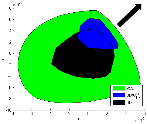
(a) LP inner approximations

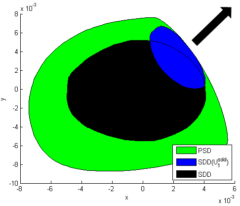
(b) SOCP inner approximations

Figure 3.1: Improvement after one Cholesky decomposition when maximizing the objective function $x+y$

An illustration of both procedures is given in Figure 3.1. We generated two random symmetric matrices $A$ and $B$ of size $10\times 10$. The outermost set is the feasible set of an SDP with the constraint $I+xA+yB\succeq 0$. The goal is to maximize the function $x+y$ over this set. The set labeled $DD$ in Figure 3.1(a) (resp. $SDD$ in Figure 3.1(b)) consists of the points $(x,y)$ for which $I+xA+yB$ is dd (resp. sdd). Let ($x_{dd}^{*},y_{dd}^{*}$) (resp. ($x_{sdd}^{*},y_{sdd}^{*}$)) be optimal solutions to the problem of maximizing $x+y$ over these sets. The set labeled $DD(U_{1}^{dd})$ in Figure 3.1(a) (resp. $SDD(U_{1}^{sdd})$ in Figure 3.1(b)) consists of the points $(x,y)$ for which $I+xA+yB\in DD(U_{1}^{d}d)$ (resp. $\in SDD(U_{1}^{sdd}$)) where $U_{1}^{dd}$ (resp. $U_{1}^{sdd}$) corresponds to the Cholesky decomposition of $I+x_{dd}^{*}A+y_{dd}^{*}B$ (resp. $I+x_{sdd}^{*}A+y_{sdd}^{*}B$). Notice the interesting phenomenon that while the new sets happen to shrink in volume, they expand in the direction that we care about. Already in one iteration, the SOCP gives the perfect bound here.

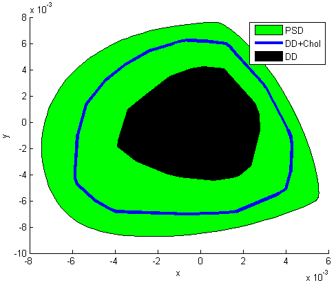
(a) LP inner approximations

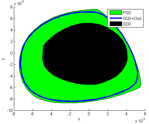
(b) SOCP inner approximations

Figure 3.2: Improvement in all directions after one Cholesky decomposition

In Figure 3.2(a), instead of showing the improvement in just the North-East direction, we show it in all directions. This is done by discretizing a large set of directions $d_{i}=(d_{i,x},d_{i,y})$ on the unit circle and optimizing along them. More concretely, for each $i$, we maximize $d_{i,x}x+d_{i,x}y$ over the set $I+xA+yB\in DD_{n}$. We extract an optimal solution every time and construct a matrix $U_{1,d_{i}}$ from its Cholesky decomposition. We then maximize in the same direction once again but this time over the set $I+xA+yB\in DD(U_{1,d_{i}})$. The set of all new optimal solutions is what is plotted with the thick blue line in the figure. We proceed in exactly the same way with our SOCPs to produce Figure 3.2(b). Notice that both inner approximations after one iteration improve substantially. The SOCP in particular fills up almost the entire spectrahedron.

3.3.2 Inner approximations to the cone of nonnegative polynomials

A problem domain where inner approximations to semidefinite programs can be useful is in sum of squares programming. This is because the goal of SOS optimization is already to inner approximate the cone of nonnegative polynomials. So by further inner approximating the SOS cone, we will get bounds in the same direction as the SOS bounds.

Let $z(x)$ be the vector of monomials of degree up to $d$. Define a family of cones of degree-$2d$ polynomials

$${DSOS(U)\mathrel{\mathop{:}}=\{p~{}|~{}p(x)=z^{T}(x)U^{T}QUz(x),\text{ for some dd matrix }Q\},}$$

parameterized by an $n\times n$ matrix $U$. We can think of this set as the cone of polynomials that are dsos in the basis $Uz(x)$. If an SOS program has a constraint “$p$ sos”, we will replace it iteratively by the constraint $p\in DSOS(U_{k})$. The sequence of matrices $\{U_{k}\}$ is again defined recursively with

$$U_{0} =I$$

$$U_{k+1} =\mbox{chol}(U_{k}^{T}Q_{k}U_{k}),$$

where $Q_{k}$ is an optimal Gram matrix of iteration $k$.

Likewise, let

$${SDSOS(U)\mathrel{\mathop{:}}=\{p~{}|~{}p(x)=z(x)^{T}U^{T}QUz(x),\text{ for some sdd matrix }Q\}.}$$

This set can also be viewed as the set of polynomials that are sdsos in the basis $Uz(x)$. To construct a sequence of SOCPs that generate improving bounds on the sos optimal value, we replace the constraint $p$ sos by $p\in SDSOS(U_{k})$, where $U_{k}$ is defined as above.

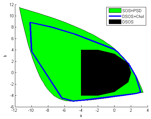
(a) LP inner approximations

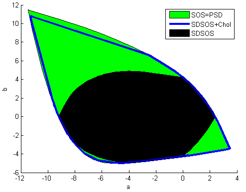
(b) SOCP inner approximations

Figure 3.3: Improvement in all directions after one Cholesky decomposition

In Figure 3.3, we consider a parametric family of polynomials

$$p_{a,b}(x_{1},x_{2})=2x_{1}^{4}+2x_{2}^{4}+ax_{1}^{3}x_{2}+(1-a)x_{2}^{2}x_{2}^{2}+bx_{1}x_{2}^{3}.$$

The outermost set in both figures corresponds to the set of pairs $(a,b)$ for which $p_{a,b}$ is sos. As $p_{a,b}$ is a bivariate quartic, this set coincides with the set of $(a,b)$ for which $p_{a,b}$ is nonnegative. The innermost sets in the two subfigures correspond to $(a,b)$ for which $p_{a,b}$ is dsos (resp. sdsos). The thick blue lines illustrate the optimal points achieved when maximizing in all directions over the sets obtained from a single Cholesky decomposition. (The details of the procedure are exactly the same as Figure 3.2.) Once again, the inner approximations after one iteration improve substantially over the DSOS and SDSOS approximations.

3.3.3 Extreme-ray interpretation of the change of basis

In this section, we present an alternative but equivalent way of expressing the LP and SOCP-based sequences. This characterization is based on the extreme-ray description of the cone of diagonally dominant/scaled diagonally dominant matrices. It will be particularly useful when we consider outer approximations of the psd cone in Section 3.3.4.

Lemma 3.3.2 (Barker and Carlson [22]).

A symmetric matrix $M$ is diagonally dominant if and only if it can be written as

$$M=\sum_{i=1}^{n^{2}}\alpha_{i}v_{i}v_{i}^{T},\alpha_{i}\geq 0,$$

where $\{v_{i}\}$ is the set of all nonzero vectors in $\mathbb{R}^{n}$ with at most $2$ nonzero components, each equal to $\pm 1$.

The vectors $v_{i}$ are the extreme rays of the $DD_{n}$ cone. This characterization of the set of diagonally dominant matrices leads to a convenient description of the dual cone:

$$DD^{*}_{n}=\{X\in{S_{n}}~{}|~{}v_{i}^{T}Xv_{i}\geq 0,i=1,\ldots,n^{2}\},$$ (3.9)

which we will find to be useful in the next subsection. Using Lemma 3.3.2, we can rewrite the sequence of LPs given in (3.5) as

$$DSOS_{k} \mathrel{\mathop{:}}=\min_{X,\alpha_{i}}C\cdot X$$ (3.10)

$$\text{s.t. }A_{i}\cdot X=b_{i},\ i=1,\ldots,m,$$

$$X=\sum_{i=1}^{n^{2}}\alpha_{i}(U_{k}^{T}v_{i})(U_{k}^{T}v_{i})^{T},$$

$${\alpha_{i}\geq 0,i=1,\ldots,n^{2}.}$$

Let $X_{k}$ be an optimal solution to the LP in iteration $k$. The sequence of matrices $\{U_{k}\}$ is defined just as before:

$$U_{0} =I$$

$$U_{k+1} =\text{chol}(X_{k}).$$

In the first iteration, a linear map is sending (or intuitively “rotating”) the extreme rays $\{v_{i}v_{i}^{T}\}$ of the dd cone to a new set of extreme rays $\{(U_{1}^{T}v_{i})(U_{1}^{T}v_{i})^{T}\}$. This procedure keeps repeating itself without ever changing the number of extreme rays.

As the sequence of LPs defined in (3.10) is equivalent to the sequence defined in (3.5), the optimal value of (3.10) improves in each iteration. This can be seen directly: Indeed, $X_{k}$ is feasible for iteration $k+1$ of (3.10) by taking $\alpha_{i}=1$ when $v_{i}$ has exactly one nonzero entry equal to $1$ and $\alpha_{i}=0$ otherwise. This automatically implies that $DSOS_{k+1}\leq DSOS_{k}.$ Moreover, the improvement is strict under the assumptions of Theorem 3.3.1.

The set of scaled diagonally dominant matrices can be described in a similar fashion. In fact, from (3.3), we know that any scaled diagonally dominant matrix $M$ can be written as

$${M=\sum_{i=1}^{{n\choose 2}}V_{i}\Lambda_{i}V_{i}^{T},}$$

where $V_{i}$ is an $n\times 2$ matrix whose columns each contain exactly one nonzero element which is equal to $1,$ and $\Lambda_{i}$ is a $2\times 2$ symmetric psd matrix.

This characterization of $SDD_{n}$ gives an immediate description of the dual cone

$$SDD^{*}_{n}={\left\{X\in S^{n}~{}|~{}V_{i}^{T}XV_{i}\succeq 0,i=1,\ldots,{n\choose 2}\right\}},$$

which will become useful later. Our SOCP sequence in explicit form is then

$$SDSOS_{k} =\min_{X,\Lambda_{i}}C\cdot X$$ (3.11)

$$\text{s.t. }A_{i}\cdot X=b_{i},i=1,\ldots,m,$$

$$X=\sum_{i=1}^{n\choose 2}(U_{k}^{T}V_{i})\Lambda_{i}(U_{k}^{T}V_{i})^{T},$$

$$\Lambda_{i}\succeq 0.$$

If $X_{k}$ is an optimal solution at step $k$, the matrix sequence $\{U_{k}\}$ is defined as before:

$$U_{0} =I$$

$$U_{k+1} =\text{chol}(X_{k}).$$

The interpretation of (3.11) is similar to that of (3.10).

3.3.4 Outer approximations of the psd cone

In Section 3.3.1, we considered inner approximations of the psd cone to obtain upper bounds on (3.4). In many applications, semidefinite programming is used as a “relaxation” to provide outer approximations to some nonconvex sets. This approach is commonly used for relaxing quadratic programs; see, e.g., Section 3.4, where we consider the problem of finding the largest stable set of a graph. In such scenarios, it does not make sense for us to inner approximate the psd cone: to have a valid relaxation, we need to outer approximate it. This can be easily achieved by working with the dual problems, which we will derive explicitly in this section.

Since $P_{n}\subseteq DD^{*}_{n}$, the first iteration in our LP sequence for outer approximation will be

$$DSOSout_{0} \mathrel{\mathop{:}}=\min_{X}C\cdot X$$

$$\text{s.t. }A_{i}\cdot X=b_{i},i=1,\ldots,m,$$

$$X\in DD_{n}^{*}.$$

By the description of the dual cone in (3.9), we know this can be equivalently written as

$$DSOSout_{0} =\min_{X}C\cdot X$$ (3.12)

$$\text{s.t. }A_{i}\cdot X=b_{i},\forall i$$

$$v_{i}^{T}Xv_{i}\geq 0,i=1,\ldots,n^{2},$$

where the $v_{i}$’s are the extreme rays of the set of diagonally dominant matrices as described in Section 3.3.3; namely, all vectors with at most two nonzero elements which are either $+1$ or $-1$. Recall that when we were after inner approximations (Subsection 3.3.1), the next LP in our sequence was generated by replacing the vectors $v_{i}$ by $U^{T}v_{i}$, where the choice of $U$ was dictated by a Cholesky decomposition of an optimal solution of the previous iterate. In the outer approximation setting, we seemingly do not have access to a psd matrix that would provide us with a Cholesky decomposition. However, we can simply get this from the dual of (3.12)

$$DSOSout^{d}_{0} \mathrel{\mathop{:}}=\max_{y,\alpha}b^{T}y$$

$$\text{s.t. }C-\sum_{i=1}^{m}y_{i}A_{i}=\sum_{i=1}^{n^{2}}\alpha_{i}v_{i}v_{i}^{T},$$

$$\alpha_{i}\geq 0,i=1,\ldots,n^{2},$$

by taking $U_{1}=\text{chol}(C-\sum_{i}y_{i}^{*}A_{i})$. We then replace $v_{i}$ by $U_{1}^{T}v_{i}$ in (3.12) to get the next iterate and proceed. In general, the sequence of LPs can be written as

$$DSOSout_{k} =\min_{X}C\cdot X$$

$$\text{s.t. }A_{i}\cdot X=b_{i},i=1,\ldots,m,$$

$$v_{i}^{T}U_{k}XU_{k}^{T}v_{i}\geq 0,$$

where $\{U_{k}\}$ is a sequence of matrices defined recursively as

$$U_{0} =I$$

$$U_{k} =\text{chol}\left(C-\sum_{i}{y_{i}^{(k-1)}}A_{i}\right).$$

The vector $y^{k-1}$ here is an optimal solution to the dual problem at step $k-1$:

$$DSOSout^{d}_{k-1} \mathrel{\mathop{:}}=\max_{y,\alpha}b^{T}y$$

$$\text{s.t. }C-\sum_{i=1}^{m}y_{i}A_{i}=\sum_{i=1}^{n^{2}}\alpha_{i}(U_{k-1}^{T}v_{i})(U_{k-1}^{T}v_{i})^{T},$$

$$\alpha_{i}\geq 0,i=1,\ldots,n^{2}.$$

This algorithm again strictly improves the objective value at each iteration. Indeed, from LP strong duality, we have

$$DSOSout_{k}=DSOSout_{k}^{d}$$

and Theorem 3.3.1 applied to the dual problem states that

$$DSOSout_{k-1}^{d}<DSOSout_{k}^{d}.$$

The sequence of SOCPs for outer approximation can be constructed in an analogous manner:

$$SDSOSout_{k} =\min_{X}C\cdot X$$

$$\text{s.t. }A_{i}\cdot X=b_{i},i=1,\ldots,m,$$

$$V_{i}^{T}U_{k}XU_{k}^{T}V_{i}\succeq 0,i=1,\ldots,{n\choose 2},$$

where $V_{i}$’s are $n\times 2$ matrices containing exactly one 1 in each column, and $\{U_{k}\}$ is a sequence of matrices defined as

$$U_{0} =I$$

$$U_{k} =\text{chol}\left(C-\sum_{i}{y_{i}^{(k-1)}}A_{i}\right)$$

Here again, the vector $y^{(k-1)}$ is an optimal solution to the dual SOCP at step $k-1$:

$$SDSOSout^{d}_{k-1} \mathrel{\mathop{:}}=\max_{y,\Lambda_{i}}b^{T}y$$

$$\text{s.t. }C-\sum_{i=1}^{m}y_{i}A_{i}=\sum_{i=1}^{n\choose 2}(U_{k-1}^{T}v_{i})\Lambda_{i}(U_{k-1}^{T}v_{i})^{T},$$

$$\Lambda_{i}\succeq 0,i=1,\ldots,{n\choose 2},$$

where each $\Lambda_{i}$ is a $2\times 2$ unknown symmetric matrix.

Remark 3.3.3.

Let us end with some concluding remarks about our algorithm. There are other ways of improving the DSOS and SDSOS bounds. For example, Ahmadi and Majumdar [9, 132] propose the requirement that $(\sum_{i=1}^{n}x_{i}^{2})^{r}p(x)$ be dsos or sdsos as a sufficient condition for nonnegativity of $p$. As $r$ increases, the quality of approximation improves, although the problem size also increases very quickly. Such hierarchies are actually commonly used in the sum of squares optimization literature. But unlike our approach, they do not take into account a particular objective function and may improve the inner approximation to the PSD cone in directions that we do not care about. Nevertheless, these hierarchies have interesting theoretical implications. Under some assumptions, one can prove that as $r\rightarrow\infty$, the underlying convex programs succeed in optimizing over the entire set of nonnegative polynomials; see, e.g., [164, 57, 152, 9].

Another approach to improve on the DSOS and SDSOS bounds appears in Chapter LABEL:chap:bp. We show there how ideas from column generation in large-scale integer and linear programming can be used to iteratively improve inner approximations to semidefinite cones. The LPs and SOCPs proposed in that work take the objective function into account and increase the problem size after each iteration by a moderate amount. By contrast, the LPs and SOCPs coming from our Cholesky decompositions in this chapter have exactly the same size in each iteration. We should remark however that the LPs from iteration two and onwards are typically more dense than the initial LP (for DSOS) and slower to solve. A worthwhile future research direction would be to systematically compare the performance of the two approaches and to explore customized solvers for the LPs and the SOCPs that arise in our algorithms.

3.4 The maximum stable set problem

A classic problem in discrete optimization is that of finding the stability number of a graph. The graphs under our consideration in this section are all undirected and unweighted. A stable set (or independent set) of a graph $G=(V,E)$ is a set of nodes of $G$ no two of which are adjacent. The stability number of $G$, often denoted by $\alpha(G)$, is the size of its maximum stable set(s). The problem of determining $\alpha$ has many applications in scheduling (see, e.g., [74]) and coding theory [128]. As an example, the maximum number of final exams that can be scheduled on the same day at a university without requiring any student to take two exams is given by the stability number of a graph. This graph has courses IDs as nodes and an edge between two nodes if and only if there is at least one student registered in both courses. Unfortunately, the problem of testing whether $\alpha(G)$ is greater than a given integer $k$ is well known to be NP-complete [102]. Furthermore, the stability number cannot be approximated within a factor $|V|^{1-\epsilon}$ for any $\epsilon>0$ unless P$=$NP [86].

A straightforward integer programming formulation of $\alpha(G)$ is given by

$$\alpha(G) =\max\sum_{i}x_{i}$$

$$\text{s.t. }x_{i}+x_{j}\leq 1,\text{ if }{\{i,j\}}\in E$$

$$x_{i}\in\{0,1\}.$$

The standard LP relaxation for this problem is obtained by changing the binary constraint $x_{i}\in\{0,1\}$ to the linear constraint $x_{i}\in[0,1]$:

$$LP \mathrel{\mathop{:}}=\max\sum_{i}x_{i}$$ (3.13)

$$\text{s.t. }x_{i}+x_{j}\leq 1,\text{ if }{\{i,j\}}\in E$$

$$x_{i}\in[0,1].$$

Solving this LP results in an upper bound on the stability number. The quality of this upper bound can be improved by adding the so-called clique inequalities. The set of $k$-clique inequalities, denoted by $C_{k}$, is the set of constraints of the type $x_{i_{1}}+x_{i_{2}}+\ldots+x_{i_{k}}\leq 1$, if $(i_{1},\ldots,i_{k})$ form a clique (i.e., a complete subgraph) of $G$. Observe that these inequalities must be satisfied for binary solutions to the above LP, but possibly not for fractional ones. Let us define a family of LPs indexed by $k$:

$$LP^{k} \mathrel{\mathop{:}}=\max\sum_{i}x_{i}$$ (3.14)

$$x_{i}\in[0,1]$$

$$C_{1},\ldots,C_{k}\text{ are satisfied.}$$

Note that $LP=LP^{2}$ by construction and $\alpha(G)\leq LP^{k+1}\leq LP^{k}$ for all $k$. We will be comparing the bound obtained by some of these well-known LPs with those achieved via the new LPs that we propose further below.

A famous semidefinite programming based upper bound on the stability number is due to Lovász [128]:

$$\vartheta(G) \mathrel{\mathop{:}}=\max_{X}J\cdot X$$

$$\text{s.t. }I\cdot X=1$$

$$X_{ij}=0,~{}\forall{\{i,j\}}\in E$$

$$X\succeq 0,$$

where $J$ here is the all ones matrix and $I$ is the identity matrix. The optimal value $\vartheta(G)$ is called the Lovász theta number of the graph. We have the following inequalities

$$\alpha(G)\leq\vartheta(G)\leq LP^{k},\ \forall k.$$

The fact that $\alpha(G)\leq\vartheta(G)$ is easily seen by noting that if $S$ is a stable set of maximum size and $1_{S}$ is its indicator vector, then the rank-one matrix $\frac{1}{|S|}1_{S}1_{S}^{T}$ is feasible to the SDP and gives the objective value $|S|$. The other inequality states that this SDP-based bound is stronger than the aforementioned LP bound even with all the clique inequalities added (there are exponentially many). A proof can be found e.g. in [116, Section 6.5.2].

Our goal here is to obtain LP and SOCP based sequences of upper bounds on the Lovász theta number. To do this, we construct a series of outer approximations of the set of psd matrices as described in Section 3.3.4. The first bound in the sequence of LPs is given by:

$$DSOS_{0}(G) \mathrel{\mathop{:}}=\max_{X}J\cdot X$$

$$\text{s.t. }I\cdot X=1$$

$$X_{ij}=0,~{}\forall{\{i,j\}}\in E$$

$$X\in DD_{n}^{*}.$$

In view of (3.9), this LP can be equivalently written as

$$DSOS_{0}(G) =\max_{X}J\cdot X$$ (3.15)

$$\text{s.t. }I\cdot X=1$$

$$X_{ij}=0,~{}\forall{\{i,j\}}\in E$$

$$v_{i}^{T}Xv_{i}\geq 0,i=1,\ldots,n^{2},$$

where $v_{i}$ is a vector with at most two nonzero entries, each nonzero entry being either $+1$ or $-1$. This LP is always feasible (e.g., with $X=\frac{1}{n}I$). Furthermore, it is bounded above. Indeed, the last constraints in (3.15) imply in particular that for all $i,j$, we must have

$$X_{i,j}\leq\frac{1}{2}(X_{ii}+X_{jj}).$$

This, together with the constraint $I\cdot X=1$, implies that the objective $J\cdot X$ must remain bounded. As a result, the first LP in our iterative sequence will give a finite upper bound on $\alpha$.

To progress to the next iteration, we will proceed as described in Section 3.3.4. The new basis for solving the problem is obtained through the dual of (3.15):

$$DSOS_{0}^{d}(G) \mathrel{\mathop{:}}=\max y$$ (3.16)

$$\text{s.t. }yI+Y-J=\sum_{i=1}^{n^{2}}\alpha_{i}v_{i}v_{i}^{T}$$

$$Y_{ij}=0\text{ if }i=j\text{ or }{\{i,j\}}\notin E$$

$$\alpha_{i}\geq 0,i=1,\ldots,n^{2}.$$

The second constraint in this problem is equivalent to requiring that $yI+Y-J$ be dd. We can define

$$U_{1}=\text{chol}(y_{0}^{*}I+Y_{0}^{*}-J)$$

where $(y_{1}^{*},Y_{1}^{*})$ are optimal solutions to (3.16). We then solve

$$DSOS_{1}(G) \mathrel{\mathop{:}}=\max_{X}J\cdot X$$

$$\text{s.t. }I\cdot X=1$$

$$X_{ij}=0,~{}\forall{\{i,j\}}\in E$$

$$v_{i}^{T}U_{1}XU_{1}^{T}v_{i}\geq 0,i=1,\ldots,n^{2},$$

to obtain our next iterate. The idea remains exactly the same for a general iterate $k$: We construct the dual

$$DSOS_{k}^{d}(G) \mathrel{\mathop{:}}=\max y$$

$$\text{s.t. }yI+Y-J=\sum_{i=1}^{n^{2}}\alpha_{i}U_{k}^{T}v_{i}(U_{k}^{T}v_{i})^{T}$$

$$Y_{ij}=0\text{ if }i=j\text{ or }{\{i,j\}}\notin E$$

$$\alpha_{i}\geq 0,\forall i,$$

and define

$$U_{k+1}\mathrel{\mathop{:}}=\text{chol}(y_{k}^{*}+Y_{k}^{*}-J),$$

where $(y_{k}^{*},Y_{k}^{*})$ is an optimal solution to the dual. The updated primal is then

$$DSOS_{k+1}(G) \mathrel{\mathop{:}}=\max_{X}J\cdot X$$ (3.17)

$$\text{s.t. }I\cdot X=1$$

$$X_{ij}=0,~{}\forall{\{i,j\}}\in E$$

$$v_{i}^{T}U_{k+1}XU_{k+1}^{T}v_{i}\geq 0,i=1,\ldots,n^{2}.$$

As stated in Section 3.3.4, the optimal values of (3.17) are guaranteed to strictly improve as a function of $k$. Note that to get the bounds, we can just work with the dual problems throughout.

An analoguous technique can be used to obtain a sequence of SOCPs. For the initial iterate, instead of requiring that $X\in DD^{*}$ in (3.15), we require that $X\in SDD^{*}$. This problem must also be bounded and feasible as

$$P_{n}\subseteq SDD^{*}\subseteq DD^{*}.$$

Then, for a given iterate $k$, the algorithm consists of solving

$$SDSOS_{k}(G) \mathrel{\mathop{:}}=\max_{X}J\cdot X$$

$$\text{s.t. }I\cdot X=1$$

$$X_{ij}=0,\forall{\{i,j\}}\in E$$

$$V_{i}^{T}U_{k}XU_{k}^{T}V_{i}\succeq 0,i=1,\ldots,{n\choose 2},$$

where as explained in Section 3.3.3 each $V_{i}$ is an $n\times 2$ matrix whose columns contain exactly one nonzero element which is equal to $1$. The matrix $U_{k}$ here is fixed and obtained by first constructing the dual SOCP

$$SDSOS_{k}^{d}(G) \mathrel{\mathop{:}}=\max y$$

$$\text{s.t. }yI+Y-J=\sum_{i=1}^{n\choose 2}U_{k}^{T}V_{i}\Lambda_{i}(U_{k}^{T}V_{i})^{T}$$

$$Y_{ij}=0\text{ if }i=j\text{ or }{\{i,j\}}\notin E$$

$$\Lambda_{i}\succeq 0,\forall i,$$

(each $\Lambda_{i}$ is a symmetric $2\times 2$ matrix decision variable) and then taking

$$U_{k}=\text{chol}(y_{k}^{*}I+Y_{k}^{*}-J).$$

Once again, one can just work with the dual problems to obtain the bounds.

As our first example, we apply both techniques to the problem of finding the stability number of the complement of the Petersen graph (see Figure 3.4(a)). The exact stability number here is 2 and an example of a maximum stable set is illustrated by the two white nodes in Figure 3.4(a). The Lovász theta number is 2.5 and has been represented by the continuous line in Figure 3.4(b). The dashed lines represent the optimal values of the LP and SOCP-based sequences of approximations for 7 iterations. Notice that already within one iteration, the optimal values are within one unit of the true stability number, which is good enough for knowing the exact bound (the stability number is an integer). From the fifth iteration onwards, they differ from the Lovász theta number by only $10^{-2}$.

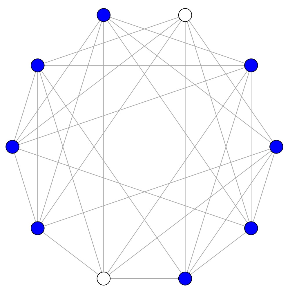
(a) Complement of Petersen graph

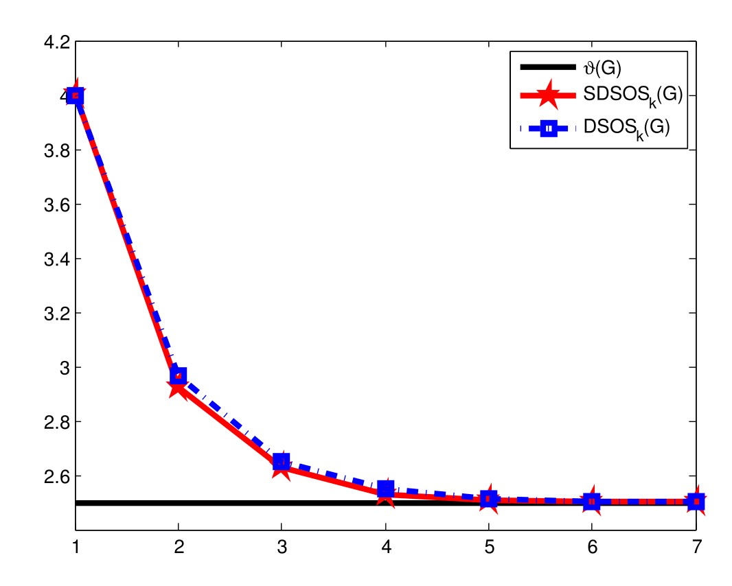
(b) The Lovász theta number and iterative bounds bounds obtained by LP and SOCP

Figure 3.4: Upper bounding the stability number of the complement of the Petersen graph

Finally, in Table 3.1, we have generated 100 instances of 20-node Erdös-Rényi graphs with edge probability $0.5$. For each instance, we compute the bounds from the Lovász SDP, the standard LP in (3.13), the standard LP with all 3-clique inequalities added ($LP^{3}$ in (3.14)), and our LP/SOCP iterative sequences. We focus here on iterations 3,4 and 5 because there is no need to go further. We compare our bounds with the standard LP and the standard LP with 3-clique inequalities because they are LPs of roughly the same size. If any of these bounds are within one unit of the true stable set number, we count this as a success and increment the counter. As can be seen in Table 3.1, the Lovász theta number is always within a unit of the stable set number, and so are our LP and SOCP sequences ($DSOS_{k},SDSOS_{k}$) after four or at most five iterations. If we look just at the bound after 3 iterations, the success rate of SDSOS is noticeably higher than the success rate of DSOS. Also note that the standard LP with or without the three clique inequalities never succeeds in giving a bound within one unit of $\alpha(G)$.

$\vartheta(G)$	$LP$	$LP^{3}$	$DSOS_{3}$	$DSOS_{4}$	$DSOS_{5}$	$SDSOS_{3}$	$SDSOS_{4}$	$SDSOS_{5}$
100%	0%	0%	14%	83%	100%	69%	100%	100%

Table 3.1: Percentage of instances out of 100 where the bound obtained is less than a unit away from the stability number

3.5 Partition

The partition problem is arguably the simplest NP-complete problem to state: Given a list of positive integers $a_{1},\ldots,a_{n}$, is it possible to split them into two sets with equal sums? We say that a partition instance is feasible if the answer is yes (e.g., {5,2,1,6,3,8,5,4,1,1,10}) and infeasible if the answer is no (e.g., {47,20,13,15,36,7,46}). The partition problem is NP-complete but only weakly. In fact, the problem admits a pseudopolynomial time algorithm based on dynamic programming that can deal with rather large problem sizes efficiently. This algorithm has polynomial running time on instances where the bit size of the integers $a_{i}$ are bounded by a polynomial in $\log n$ [71]. In this section, we investigate the performance and mostly limitations of algebraic techniques for refuting feasibility of partition instances.

Feasibility of a partition instance can always be certified by a short proof (the partition itself). However, unless P=co-NP, we do not expect to always have short certificates of infeasibility. Nevertheless, we can try to look for such a certificate through a sum of squares decomposition. Indeed, given an instance $a\mathrel{\mathop{:}}=\{a_{1},\ldots,a_{n}\}$, it is not hard to see that the following equivalence holds:

$${\begin{bmatrix}a\text{ is an infeasible }\\ \text{ partition instance}\end{bmatrix}}\Leftrightarrow p_{a}(x)\mathrel{\mathop{:}}=\sum_{i}(x_{i}^{2}-1)^{2}+(\sum_{i}a_{i}x_{i})^{2}>0,~{}\forall x\in\mathbb{R}^{n}.$$ (3.18)

So if for some $\epsilon>0$ we could prove that $p_{a}(x)-\epsilon$ is nonnegative, we would have refuted the feasibility of our partition instance.

Definition 3.5.1.

An instance of partition $a_{1},\ldots,a_{n}$ is said to be sos-refutable if there exists $\epsilon>0$ such that $p_{a}(x)-\epsilon$ is sos.

Obviously, any instance of partition that is sos-refutable is infeasible. This suggests that we can consider solving the following semidefinite program

$$SOS \mathrel{\mathop{:}}=\max\ \epsilon$$ (3.19)

$$\text{s.t. }q_{a}(x)\mathrel{\mathop{:}}=p_{a}(x)-\epsilon\text{ is sos}$$

and examining its optimal value. Note that the optimal value of this problem is always greater than or equal to zero as $p_{a}$ is sos by construction. If the optimal value is positive, we have succeeded in proving infeasibility of the partition instance $a$.

We would like to define the notions of dsos-refutable and sdsos-refutable instances analogously by replacing the condition $q_{a}(x)$ sos by the condition $q_{a}(x)$ dsos or sdsos. Though (3.19) is guaranteed to always be feasible by taking $\epsilon=0$, this is not necessarily the case for dsos/sdsos versions of (3.19). For example, the optimization problem

$$\max_{\epsilon}\{\epsilon~{}|~{}p_{a}(x)-\epsilon\text{ dsos}\}$$ (3.20)

on the instance $\{1,2,2,1,1\}$ is infeasible. This is a problem for us as we need the first LP to be feasible to start our iterations. We show, however, that we can get around this issue by modeling the partition problem with homogeneous polynomials.

Definition 3.5.2.

Let $p_{a}$ be as in (3.18). An instance of partition $a_{1},\ldots,a_{n}$ is said to be dsos-refutable (resp. sdsos-refutable) if there exists $\epsilon>0$ such that the quartic form

$$q_{a,\epsilon}^{h}(x)\mathrel{\mathop{:}}=p_{a}\left(\frac{x}{\left(\frac{1}{n}\sum_{i}x_{i}^{2}\right)^{1/2}}\right)\left(\frac{1}{n}\sum_{i}x_{i}^{2}\right)^{2}-\epsilon\left(\frac{1}{n}\sum_{i}x_{i}^{2}\right)^{2}$$ (3.21)

is dsos (resp. sdsos).

Notice that $q_{a,\epsilon}^{h}$ is indeed a polynomial as it can be equivalently written as

$$\sum_{i}x_{i}^{4}+\left(\left(\sum_{i}a_{i}x_{i}\right)^{2}-2\sum_{i}x_{i}^{2}\right)\cdot\left(\frac{1}{n}\sum_{i}x_{i}^{2}\right)+(n-\epsilon)\cdot\left(\frac{1}{n}\sum_{i}x_{i}^{2}\right)^{2}.$$

What we are doing here is homogenizing a polynomial that does not have odd monomials by multiplying its lower degree monomials with appropriate powers of $\sum_{i}x_{i}^{2}$. The next theorem tells us how we can relate nonnegativity of this polynomial to feasibility of partition.

Theorem 3.5.3.

A partition instance $a=\{a_{1},\ldots,a_{n}\}$ is infeasible if and only if there exists $\epsilon>0$ for which the quartic form $q_{a,\epsilon}^{h}(x)$ defined in (3.21) is nonnegative.

Proof.

For ease of reference, let us define

$$p_{a}^{h}(x)\mathrel{\mathop{:}}=p_{a}\left(\frac{x}{\left(\frac{1}{n}\sum_{i}x_{i}^{2}\right)^{1/2}}\right)\left(\frac{1}{n}\sum_{i}x_{i}^{2}\right)^{2}.$$ (3.22)

Suppose partition is feasible, i.e, the integers $a_{1},\ldots,a_{n}$ can be placed in two sets $\mathcal{S}_{1}$ and $\mathcal{S}_{2}$ with equal sums. Let $\bar{x}_{i}$=1 if $a_{i}$ is placed in set $\mathcal{S}_{1}$ and $\bar{x}_{i}=-1$ if $a_{i}$ is placed in set $\mathcal{S}_{2}$. Then $||\bar{x}||_{2}^{2}=n$ and $p_{a}(\bar{x})=0$. This implies that

$$p_{a}^{h}(\bar{x})=p_{a}(\bar{x})=0,$$

and hence having $\epsilon>0$ would make

$$q_{a,\epsilon}^{h}(\bar{x})=-\epsilon<0.$$

If partition is infeasible, then $p_{a}(x)>0,~{}\forall x\in\mathbb{R}^{n}$. In view of (3.22) we see that $p_{a}^{h}(x)>0$ on the sphere $\mathbb{S}$ of radius $n$. Since $p_{a}^{h}$ is continuous, its minimum $\hat{\epsilon}$ on the compact set $\mathbb{S}$ is achieved and must be positive. So we must have

$$q_{a,\hat{\epsilon}}^{h}(x)=p_{a}^{h}(x)-\hat{\epsilon}\left(\frac{1}{n}\sum_{i}x_{i}^{2}\right)^{2}\geq 0,\forall x\in\mathbb{S}.$$

By homogeneity, this implies that $q_{a,\hat{\epsilon}}^{h}$ is nonnegative everywhere. ∎

Consider now the LP

$$\max_{\epsilon}\ \epsilon$$ (3.23)

$$\text{s.t. }q_{a,\epsilon}^{h}(x)\ \text{dsos.}$$

Theorem 3.5.4.

The LP in (3.23) is always feasible.

Proof.

Let $h(x)\mathrel{\mathop{:}}=\left(\frac{1}{n}\sum_{i}x_{i}^{2}\right)^{2}$ and recall that $z(x,2)$ denotes the vector of all monomials of degree exactly $2$. We can write

$$h(x)=z^{T}(x,2)Q_{h}z(x,2)$$

where $Q_{h}$ is in the strict interior of the $DD_{n}$ cone (i.e., its entries $q_{ij}$ satisfy $q_{ii}>\sum_{j}|q_{ij}|,\forall i$). Furthermore, let $Q$ be a symmetric matrix such that $p_{a}^{h}(x)=z(x,2)^{T}Qz(x,2).$ Then

$$q_{a,\epsilon}^{h}(x)=p_{a}^{h}(x)-\epsilon h(x)=z(x,2)^{T}(Q-\epsilon Q_{h})z(x,2).$$

As $Q_{h}$ is in the strict interior of $DD_{n}$, $\exists\lambda>0$ such that

$$\lambda Q+(1-\lambda)Q_{h}\text{ is dd.}$$

Taking $\epsilon=-\frac{1-\lambda}{\lambda}$, $Q-\epsilon Q_{h}$ will be diagonally dominant and $q_{a,\epsilon}^{h}$ will be dsos. ∎

As an immediate consequence, the SOCP

$$\max_{\epsilon}\ \epsilon$$ (3.24)

$$\text{s.t. }q_{a,\epsilon}^{h}(x)\text{ sdsos}$$

is also always feasible. We can now define our sequence of LPs and SOCPs as we have guaranteed feasibility of the first iteration. This is done following the strategy and notation of Section 3.3.2:

$$DSOS_{k}\text{ (resp. $SDSOS_{k}$)} \mathrel{\mathop{:}}=\max_{\epsilon}\ \epsilon$$ (3.25)

$$\text{s.t. }q_{a,\epsilon}^{h}(x)\in DSOS(U_{k})\text{ (resp. $SDSOS(U_{k})$)},$$

where $\{U_{k}\}$ is a sequence of matrices recursively defined with $U_{0}=I$ and $U_{k+1}$ defined as the Cholesky factor of an optimal dd (resp. sdd) Gram matrix of the optimization problem in iteration $k$.

We illustrate the performance of these LP and SOCP-based bounds on the infeasible partition instance $\{1,2,2,1,1\}$. The results are in Figure 3.5. We can use the sum of squares relaxation to refute the feasibility of this instance by either solving (3.19) (the “non-homogenized version”) or solving (3.23) with dsos replaced with sos (the “homogenized version”). Both approaches succeed in refuting this partition instance, though the homogenized version gives a slightly better (more positive) optimal value. As a consequence, we only plot the homogeneous bound, denoted by $SOS_{h}$, in Figure 3.5. Notice that the LP and SOCP-based sequences refute the instance from the $6^{th}$ iteration onwards.

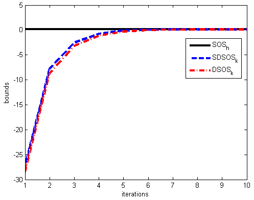
(a) Bounds $SOS_{h}$, $DSOS_{k}$ and $SDSOS_{k}$

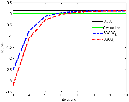
(b) Zoomed-in version of Figure 3.5(a)

Figure 3.5: Bounds obtained on the {1,2,2,1,1} instance of the partition problem using SDP, as well as the LP/SOCP-based sequences

As our final experiment, we generate 50 infeasible instances of partition with 6 elements randomly generated between 1 and 15. These instances are trivially infeasible because we made sure that $a_{1}+\cdots+a_{6}$ is an odd number. In the first column of Table 3.2, we count the number of successes for sos-refutability (non homogeneous version as defined in Definition 3.5.1), where a failure is defined as the optimal value of (3.19) being 0 up to numerical precision. The second column corresponds to the number of successes for sos-refutability (homogeneous version). The last 4 columns show the success rate of the LP and SOCP-based sequences as defined in (3.25), after 20 iterations and 40 iterations.

$SOS$	$SOS_{h}$	$DSOS_{20}$	$DSOS_{40}$	$SDSOS_{20}$	$SDSOS_{40}$
56%	56%	12%	16 %	14%	14%

Table 3.2: Rate of success for refutability of infeasible instances of partition

From the experiments, the homogeneous and non-homogeneous versions of (3.19) have the same performance in terms of their ability to refute feasibility. However, we observe that they both fail to refute a large number of completely trivial instances! We prove why this is the case for one representative instance in the next section. The LP and SOCP-based sequences also perform poorly and their convergence is much slower than what we observed for the maximum stable set problem in Section 3.4.

3.5.1 Failure of the sum of squares relaxation on trivial partition instances.

For complexity reasons, one would expect there to be infeasible instances of partition that are not sos-refutable. What is surprising however is that the sos relaxation is failing on many instances that are totally trivial to refute as the sum of their input integers is odd. We present a proof of this phenomenon on an instance which is arguably the simplest one.

Proposition 3.5.5.

The infeasible partition instance $\{1,1,1,1,1\}$ is not sos-refutable.

Proof.

Let $p_{a}$ be the polynomial defined in (3.18). To simplify notation, we let $p(x)$ represent $p_{a}(x)$ for $a=\{1,1,1,1,1\}$. We will show that $p$ is on the boundary of the SOS cone even though we know it is strictly inside the PSD cone. This is done by presenting a dual functional $\mu$ that vanishes on $p,$ takes a nonnegative value on all quartic sos polynomials, and a negative value on $p(x)-\epsilon$ for any $\epsilon>0.$ (See Figure 3.6 for an intuitive illustration of this.)

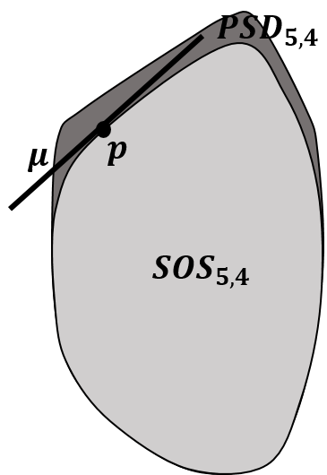
Figure 3.6: The geometric idea behind the proof of Proposition 3.5.5

The polynomial $p$ when expanded out reads

$$p(x)=n-\sum_{i}x_{i}^{2}+2\sum_{i<j}x_{i}x_{j}+\sum_{i}x_{i}^{4}.$$ (3.26)

Consider the vector of coefficients of $p$ with the ordering as written in (3.26):

$$\overrightarrow{p}=\setcounter{MaxMatrixCols}{21}\begin{pmatrix}5&-1&-1&-1&-1&-1&2&2&2&2&2&2&2&2&2&2&-1&-1&-1&-1&-1\end{pmatrix}.$$ (3.27)

This is a reduced representation of the vector of coefficients of $p$, in that there are many zeros associated with all other monomials of degree less than or equal to 4, which we are not writing out.

Our goal is to find a vector $\mu$ that satisfies

$$\langle\mu,\overrightarrow{p}\rangle =0$$

$$\langle\mu,\overrightarrow{q}\rangle \geq 0,\text{ for all $q$ sos of degree 4}.$$ (3.28)

If such a $\mu$ exists and its first element is nonzero (which by rescaling can then be taken to be 1), then $\langle\mu,\overrightarrow{p-\epsilon}\rangle=\langle\mu,\overrightarrow{p}\rangle-\langle\mu,\overrightarrow{\epsilon}\rangle=-\epsilon<0$. This provides us with the required functional that separates $p(x)-\epsilon$ from the set of sos polynomials.

Selecting the same reduced basis as the one used in (3.27), we take

$$\overrightarrow{\mu_{reduced}}=\begin{pmatrix}1&\textbf{1}_{5}^{T}&-\frac{1}{4}\cdot\textbf{1}_{1}^{T}&\textbf{1}_{5}^{T}\end{pmatrix}$$

where $\textbf{1}_{n}$ is the all ones vector of size $n$. The subscript “reduced” denotes the fact that in $\overrightarrow{\mu_{reduced}}$, only the elements of $\mu$ needed to verify $\langle\mu,\overrightarrow{p}\rangle=0$ are presented. Unlike $\overrightarrow{p}$, the entries of $\mu$ corresponding to the other monomials are not all zero. This can be seen from the entries of the matrix $M$ that appears further down.

We now show how (3.28) holds. Consider any sos polynomial $q$ of degree less than or equal to 4. We know that it can be written as

$$q(x)=z^{T}Qz=\mbox{Tr}~{}Q\cdot zz^{T},$$

for some $Q\succeq 0$, and a vector of monomials

$$z^{T}=[1,x_{1},x_{2},\ldots,x_{n},x_{1}^{2},\ldots,x_{n}^{2},x_{1}x_{2},\ldots,x_{n-1}x_{n}].$$

It is not difficult to see that

$$\langle\mu,\overrightarrow{q}\rangle=\mbox{Tr}~{}Q\cdot(zz^{T})|_{\mu}$$

where by $(zz)^{T}|_{\mu}$, we mean a matrix where each monomial in $zz^{T}$ is replaced with the corresponding element of the vector $\mu$. This yields the matrix

$$M=\setcounter{MaxMatrixCols}{21}\begin{pmatrix}1&0&0&0&0&0&1&1&1&1&1&b&b&b&b&b&b&b&b&b&b\\ 0&1&b&b&b&b&0&0&0&0&0&0&0&0&0&0&0&0&0&0&0\\ 0&b&1&b&b&b&0&0&0&0&0&0&0&0&0&0&0&0&0&0&0\\ 0&b&b&1&b&b&0&0&0&0&0&0&0&0&0&0&0&0&0&0&0\\ 0&b&b&b&1&b&0&0&0&0&0&0&0&0&0&0&0&0&0&0&0\\ 0&b&b&b&b&1&0&0&0&0&0&0&0&0&0&0&0&0&0&0&0\\ 1&0&0&0&0&0&1&1&1&1&1&b&b&b&b&b&b&b&b&b&b\\ 1&0&0&0&0&0&1&1&1&1&1&b&b&b&b&b&b&b&b&b&b\\ 1&0&0&0&0&0&1&1&1&1&1&b&b&b&b&b&b&b&b&b&b\\ 1&0&0&0&0&0&1&1&1&1&1&b&b&b&b&b&b&b&b&b&b\\ 1&0&0&0&0&0&1&1&1&1&1&b&b&b&b&b&b&b&b&b&b\\ b&0&0&0&0&0&b&b&b&b&b&1&b&b&b&b&b&b&a&a&a\\ b&0&0&0&0&0&b&b&b&b&b&b&1&b&b&b&a&a&b&b&a\\ b&0&0&0&0&0&b&b&b&b&b&b&b&1&b&a&b&a&b&a&b\\ b&0&0&0&0&0&b&b&b&b&b&b&b&b&1&a&a&b&a&b&b\\ b&0&0&0&0&0&b&b&b&b&b&b&b&a&a&1&b&b&b&b&a\\ b&0&0&0&0&0&b&b&b&b&b&b&a&b&a&b&1&b&b&a&b\\ b&0&0&0&0&0&b&b&b&b&b&b&a&a&b&b&b&1&a&b&b\\ b&0&0&0&0&0&b&b&b&b&b&a&b&b&a&b&b&a&1&b&b\\ b&0&0&0&0&0&b&b&b&b&b&a&b&a&b&b&a&b&b&1&b\\ b&0&0&0&0&0&b&b&b&b&b&a&a&b&b&a&b&b&b&b&1\\ \end{pmatrix},$$

where $a=\frac{3}{8}$ and $b=-\frac{1}{4}$. We can check that $M\succeq 0$. This, together with the fact that $Q\succeq 0,$ implies that (3.28) holds. ∎

3.5.2 Open problems

We showed in the previous subsection that the infeasible partition instance $\{1,1,1,1,1\}$ was not sos-refutable. Many more randomly-generated partition instances that we knew to be infeasible (their sum being odd) also failed to be sos-refutable. This observation motivates the following open problem:

Open Problem 1

Characterize the set of partition instances $\{a_{1},\ldots,a_{n}\}$ that have an odd sum but are not sos-refutable (see Definition 3.5.1).

Our second open problem has to do with the power of higher order sos relaxations for refuting feasibility of partition instances.

Open Problem 2

For a positive integer $r$, let us call a partition instance $\{a_{1},\ldots,a_{n}\}$ $r$-sos-refutable if $\exists\epsilon>0$ such that $(p(x)-\epsilon)(\sum_{i}x_{i}^{2}+1)^{r}$ is sos. Note that this is also a certificate of infeasibility of the instance. Even though the $\{1,1,1,1,1\}$ instance is not sos-refutable, it is $1$-sos-refutable. Furthermore, we have numerically observed that the instance $\{1,1,1,1,1,1,1\}$ (vector of all ones of length 7) is not sos-refutable or $1$-sos-refutable, but it is $2$-sos-refutable. If we consider the instance consisting of $n$ ones with $n$ odd, and define $\tilde{r}$ to be the minimum $r$ such that $\{1,1,\ldots,1\}$ becomes $r$-sos-refutable, is it true that $\tilde{r}$ must grow with $n$?

Chapter 4 On the Construction of Converging Hierarchies for Polynomial Optimization Based on Certificates of Global Positivity

4.1 Introduction

A polynomial optimization problem (POP) is an optimization problem of the form

$$\inf_{x\in\mathbb{R}^{n}} p(x)$$ (4.1)

s.t. $$g_{i}(x)\geq 0,~{}i=1,\ldots,m,$$

where $p,g_{i},~{}i=1,\ldots,m,$ are polynomial functions in $n$ variables $x\mathrel{\mathop{:}}=(x_{1},\ldots,x_{n})$ and with real coefficients. It is well-known that polynomial optimization is a hard problem to solve in general. For example, simply testing whether the optimal value of problem (4.1) is smaller than or equal to some rational number $k$ is NP-hard already when the objective is quadratic and the constraints are linear [151]. Nevertheless, these problems remain topical due to their numerous applications throughout engineering, operations research, and applied mathematics (see, e.g., [111, 30, 8]). In this chapter, we are interested in obtaining lower bounds on the optimal value of problem (4.1). We focus on a class of methods which construct hierarchies of tractable convex optimization problems whose optimal values are lowerbounds on the optimal value of (4.1), with convergence to it as the sequence progresses. This implies that even though the original POP is nonconvex, one can obtain increasingly accurate lower bounds on its optimal value by solving convex optimization problems. One method for constructing these hierarchies of optimization problems that has gained attention in recent years relies on the use of Positivstellensätze (see, e.g., [115] for a survey). Positivstellensätze are algebraic identities that certify infeasibility of a set of polynomial inequalities, or equivalently, positivity of a polynomial on a basic semialgebraic set. (Recall that a basic semialgebraic set is a set defined by finitely many polynomial inequalities.) These Positivstellensätze can be used to prove lowerbounds on POPs. Indeed, if we denote the feasible set of (4.1) by $S$, the optimal value of problem (4.1) is equivalent to

$$\sup_{\gamma} \gamma$$ (4.2)

s.t. $$p(x)-\gamma\geq 0,~{}\forall x\in S.$$

Hence if $\gamma$ is a strict lower bound on (4.1), we have that $p(x)-\gamma>0$ on $S$, a fact that can be certified using Positivstellensätze. At a conceptual level, hierarchies that provide lower bounds on (4.1) are constructed thus: we fix the “size of the certificate” at each level of the hierarchy and search for the largest $\gamma$ such that the Positivstellensätze at hand can certify positivity of $p(x)-\gamma$ over $S$ with a certificate of this size. As the sequence progresses, we increase the size of the certificates allowed, hence obtaining increasingly accurate lower bounds on (4.1).

Below, we present three of the better-known Positivstellensätze, given respectively by Stengle [181], Schmüdgen [173], and Putinar [162]. These all rely on sum of squares certificates. We recall that a polynomial is a sum of squares (sos) if it can be written as a sum of squares of other polynomials. We start with Stengle’s Positivstellensatz, which certifies infeasibility of a set of polynomial inequalities. It is sometimes referred to as “the Positivstellensatz” in related literature as it requires no assumptions, contrarily to Schmüdgen and Putinar’s theorems which can be viewed as refinements of Stengle’s result under additional assumptions.

Theorem 4.1.1 (Stengle’s Positivstellensatz [181]).

The basic semialgebraic set

$$S=\{x\in\mathbb{R}^{n}~{}|~{}g_{1}(x)\geq 0,\ldots,g_{m}(x)\geq 0\}$$

is empty if and only if there exist sum of squares polynomials $s_{0}(x)$,$s_{1}(x)$,$\ldots$, $s_{m}(x)$, $s_{12}(x)$, $s_{13}(x)$,$\ldots$, $s_{123\ldots m}(x)$ such that

$$-1=s_{0}(x)+\sum_{i}s_{i}(x)g_{i}(x)+\sum_{\{i,j\}}s_{ij}(x)g_{i}(x)g_{j}(x)+\ldots+s_{123\ldots m}(x)g_{1}(x)\ldots g_{m}(x).$$

The next two theorems, due to Schmüdgen and Putinar, certify positivity of a polynomial $p$ over a basic semialgebraic set $S$. They impose additional compactness assumptions comparatively to Stengle’s Positivstellensatz.

Theorem 4.1.2 (Schmüdgen’s Positivstellensatz [173]).

Assume that the set

$$S=\{x\in\mathbb{R}^{n}~{}|~{}g_{1}(x)\geq 0,\ldots,g_{m}(x)\geq 0\}$$

is compact. If a polynomial $p$ is positive on $S$, then

$$p(x)=s_{0}(x)+\sum_{i}s_{i}(x)g_{i}(x)+\sum_{\{i,j\}}s_{ij}(x)g_{i}(x)g_{j}(x)+\ldots+s_{123\ldots m}(x)g_{1}(x)\ldots g_{m}(x),$$

where $s_{0}(x)$,$s_{1}(x)$,$\ldots$, $s_{m}(x)$, $s_{12}(x)$, $s_{13}(x)$,$\ldots$, $s_{123\ldots m}(x)$ are sums of squares.

Theorem 4.1.3 (Putinar’s Positivstellensatz [162]).

Let

$$S=\{x\in\mathbb{R}^{n}~{}|~{}g_{1}(x)\geq 0,\ldots,g_{m}(x)\geq 0\}$$

and assume that $\{g_{1},\ldots,g_{m}\}$ satisfy the Archimedean property, i.e., there exists $N\in~{}\mathbb{N}$ such that

$$N-\sum_{i}x_{i}^{2}=\sigma_{0}(x)+\sigma_{1}(x)g_{1}(x)+\ldots+\sigma_{m}(x)g_{m}(x),$$

where $\sigma_{1}(x),\ldots,\sigma_{m}(x)$ are sums of squares. If a polynomial $p$ is positive on $S$, then

$$p(x)=s_{0}(x)+s_{1}(x)g_{1}(x)+\ldots+s_{m}(x)g_{m}(x),$$

where $s_{1}(x),\ldots,s_{m}(x)$ are sums of squares.

Note that these three Positivstellensätze involve in their expressions sum of squares polynomials of unspecified degree. To construct hierarchies of tractable optimization problems for (4.2), we fix this degree: at level $r$, we search for the largest $\gamma$ such that positivity of $p(x)-\gamma$ over $S$ can be certified using the Positivstellensätze where the degrees of all sos polynomials are taken to be less than or equal to $2r$. Solving each level of these hierarchies is then a semidefinite program (SDP). This is a consequence of the fact that one can optimize over (or test membership to) the set of sum of squares polynomials of fixed degree using semidefinite programming [153, 152, 109]. Indeed, a polynomial $p$ of degree $2d$ and in $n$ variables is a sum of squares if and only if there exists a symmetric matrix $Q\succeq 0$ such that $p(x)=z(x)^{T}Qz(x)$, where $z(x)=(1,x_{1},\ldots,x_{n},\ldots,x_{n}^{d})^{T}$ is the standard vector of monomials in $n$ variables and of degree less than or equal to $d$. We remark that the hierarchy obtained from Stengle’s Positivstellensatz was proposed and analyzed by Parrilo in [153]; the hierarchy obtained from Putinar’s Positivstellensatz was proposed and analyzed by Lasserre in [109]. There have been more recent works that provide constructive proofs of Schmüdgen and Putinar’s Positivstellensätze; see [20, 175, 177]. These proofs rely on other Positivstellensätze, e.g., a result by Polyá (see Theorem 4.1.6 below) in [175, 177], and the same result by Polyá, Farkas’ lemma, and Stengle’s Positivstellensatz in [20]. There has further been an effort to derive complexity bounds for Schmüdgen and Putinar’s Positivstellensätze in recent years; see [147, 176].

On a historical note, Stengle, Schmüdgen, and Putinar’s Positivstellensätze were derived in the latter half of the 20th century. As mentioned previously, they all certify positivity of a polynomial over an arbitrary basic semialgebraic set (modulo compactness assumptions). By contrast, there are Positivstellensätze from the early 20th century that certify positivity of a polynomial globally. Perhaps the most well-known Positivstellensatz of this type is due to Artin in 1927, in response to Hilbert’s 17th problem. Artin shows that any nonnegative polynomial is a sum of squares of rational functions. Here is an equivalent formulation of this statement:

Theorem 4.1.4 (Artin [18]).

For any nonnegative polynomial $p$, there exists an sos polynomial $q$ such that $p\cdot q$ is a sum of squares.

To the best of our knowledge, in this area, all converging hierarchies of lower bounds for POPs are based off of Positivstellensätze that certify nonnegativity of a polynomial over an arbitrary basic semialgebraic set. In this chapter, we show that in fact, under compactness assumptions, it suffices to have only global certificates of nonnegativity (such as the one given by Artin) to produce a converging hierarchy for general POPs. As a matter of fact, even weaker statements that apply only to globally positive (as opposed to globally nonnegative) forms are enough to derive converging hierarchies for POPs. Examples of such statements are due to Habicht [81] and Reznick [164]. With such an additional positivity assumption, more can usually be said about the structure of the polynomial $q$ in Artin’s result. Below, we present the result by Reznick.

Theorem 4.1.5 (Reznick [164]).

For any positive definite form $p$, there exists $r\in\mathbb{N}$ such that $p(x)\cdot(\sum_{i}x_{i}^{2})^{r}$ is a sum of squares.

We show in this chapter that this Positivstellensatz also gives rise to a converging hierarchy for POPs with a compact feasible set similarly to the one generated by Artin’s Positivstellensatz.

Through their connections to sums of squares, the two hierarchies obtained using the theorems of Reznick and Artin are semidefinite programming-based. In this chapter, we also derive an “optimization-free” converging hierarchy for POPs with compact feasible sets where each level of the hierarchy only requires that we be able to test nonnegativity of the coefficients of a given fixed polynomial. To the best of our knowledge, this is the first converging hierarchy of lower bounds for POPs which does not require that convex optimization problems be solved at each of its levels. To construct this hierarchy, we use a result of Polyá [158], which just like Artin’s and Reznick’s Positivstellensätze, certifies global positivity of forms. However this result is restricted to even forms. Recall that a form $p$ is even if each of the variables featuring in its individual monomials has an even power. This is equivalent (see [54, Lemma 2]) to $p$ being invariant under change of sign of each of its coordinates, i.e.,

$$p(x_{1},\ldots,x_{n})=p(-x_{1},\ldots,x_{n})=\cdots=p(x_{1},\ldots,-x_{n}).$$

Theorem 4.1.6 (Polyá [158]).

For any positive definite even form $p$, there exists $r\in\mathbb{N}$ such that $p(x)\cdot(\sum_{i}x_{i}^{2})^{r}$ has nonnegative coefficients.

Our aforementioned hierarchy enables us to obtain faster-converging linear programming (LP) and second-order cone programming (SOCP)-based hierarchies for general POPs with compact feasible sets that rely on the concepts of dsos and sdsos polynomials. These are recently introduced inner approximations to the set of sos polynomials that have shown much better scalability properties in practice [9].

As a final remark, we wish to stress the point that the goal of this chapter is first and foremost theoretical, i.e., to provide methods for constructing converging hierarchies of lower bounds for POPs using as sole building blocks certificates of global positivity. We do not make any claims that these hierarchies can outperform the popular existing hierarchies due, e.g., to Lasserre [109] and Parrilo [153]. We do believe however that the optimization-free hierarchy presented in Section 4.4.1 could potentially be of interest in large-scale applications where the convex optimization problems appearing in traditional hierarchies are too cumbersome to solve.

4.1.1 Outline of the chapter

The chapter is structured as follows. In Section 4.2, we show that if one can inner approximate the cone of positive definite forms arbitrarily well (with certain basic properties), then one can produce a converging hierarchy of lower bounds for POPs with compact feasible sets (Theorem 4.2.4). This relies on a reduction (Theorem 4.2.1) that reduces the problem of certifying a strict lower bound on a POP to that of proving positivity of a certain form. In Section 4.3, we see how this result can be used to derive semidefinite programming-based converging hierarchies (Theorems 4.3.2 and 4.3.4) from the Positivstellensätze by Artin (Theorem 6.4.2) and Reznick (Theorem 4.1.5). In Section 4.4, we derive an optimization-free hierarchy (Theorem 4.4.1) from the Positivstellensatz of Polyá (Theorem 4.1.6) as well as LP and SOCP-based hierarchies which rely on dsos/sdsos polynomials (Corollary 4.4.8). We conclude with a few open problems in Section 4.5.

4.1.2 Notation and basic definitions

We use the standard notation $A\succeq 0$ to denote that a symmetric matrix $A$ is positive semidefinite. Recall that a form is a homogeneous polynomial, i.e., a polynomial whose monomials all have the same degree. We denote the degree of a form $f$ by $deg(f)$. We say that a form $f$ is nonnegative (or positive semidefinite) if $f(x)\geq 0$, for all $x\in\mathbb{R}^{n}$ (we write $f\geq 0$). A form $f$ is positive definite (pd) if $f(x)>0,$ for all nonzero $x$ in $\mathbb{R}^{n}$ (we write $f>0$). Throughout the chapter, we denote the set of forms (resp. the set of nonnegative forms) in $n$ variables and of degree $d$ by $H_{n,d}$ (resp $P_{n,d}$). We denote the ball of radius $R$ and centered at the origin by $B(0,R)$ and the unit sphere in $x$-space, i.e., $\{x\in\mathbb{R}^{n}~{}|~{}||x||_{2}=1\}$, by $S_{x}$. We use the shorthand $f(y^{2}-z^{2})$ for $y,z\in\mathbb{R}^{n}$ to denote $f(y_{1}^{2}-z_{1}^{2},\ldots,y_{n}^{2}-z_{n}^{2}).$ We say that a scalar $\gamma$ is a strict lower bound on (4.1) if $p(x)>\gamma,~{}\forall x\in S$. Finally, we ask the reader to carefully read Remark 4.2.3 which contains the details of a notational overwriting occurring before Theorem 4.2.4 and valid from then on throughout the chapter. This overwriting makes the chapter much simpler to parse.

4.2 Constructing converging hierarchies for POP using global certificates of positivity

Consider the polynomial optimization problem in (4.1) and denote its optimal value by $p^{*}$. Let $d$ be such that $2d$ is the smallest even integer larger than or equal to the maximum degree of $p,g_{i},i=1,\ldots,m$. We denote the feasible set of our optimization problem by

$$S=\{x\in\mathbb{R}^{n}~{}|~{}g_{i}(x)\geq 0,i=1,\ldots,m\}$$

and assume that $S$ is contained within a ball of radius $R$. From this, it is easy to provide (possibly very loose) upper bounds on $g_{i}(x)$ over the set $S$: as $S$ is contained in a ball of radius $R$, we have $|x_{i}|\leq R$, for all $i=1,\ldots,n$. We then use this to upper bound each monomial in $g_{i}$ and consequently $g_{i}$ itself. We use the notation $\eta_{i}$ to denote these upper bounds, i.e., $g_{i}(x)\leq\eta_{i}$, for all $i=1,\ldots,m$ and for all $x\in S$. Similarly, we can provide an upperbound on $-p(x)$. We denote such a bound by $\beta$, i.e., $-p(x)\leq\beta,$ $\forall x\in S.$

The goal of this section is to produce a method for constructing converging hierarchies of lower bounds for POPs if we have access to arbitrarily accurate inner approximations of the set of positive definite forms. The first theorem (Theorem 4.2.1) connects lower bounds on (4.1) to positive definiteness of a related form. The second theorem (Theorem 4.2.4) shows how this can be used to derive a hierarchy for POPs.

Theorem 4.2.1.

Consider the general polynomial optimization problem in (4.1) and recall that $d$ is such that $2d$ is the smallest even integer larger than or equal to the maximum degree of $p,g_{i},i=1,\ldots,m$. Suppose $S\subseteq B(0,R)$ for some positive scalar $R$. Let $\eta_{i},i=1,\ldots,m$ (resp. $\beta$) be any finite upper bounds on $g_{i}(x),i=1,\ldots,m$ (resp. $-p(x)$).

Then, a scalar $\gamma$ is a strict lower bound on (4.1) if and only if the homogeneous sum of squares polynomial

$$f_{\gamma}(x,s,y)\mathrel{\mathop{:}}= \left(\gamma y^{2d}-y^{2d}p(x/y)-s_{0}^{2}y^{2d-2}\right)^{2}+\sum_{i=1}^{m}\left(y^{2d}g_{i}(x/y)-s_{i}^{2}y^{2d-2}\right)^{2}$$ (4.3)

$$+\left((R+\sum_{i=1}^{m}\eta_{i}+\beta+\gamma)^{d}y^{2d}-(\sum_{i=1}^{n}x_{i}^{2}+\sum_{i=0}^{m}s_{i}^{2})^{d}-s_{m+1}^{2d}\right)^{2}$$

of degree $4d$ and in $n+m+3$ variables $(x_{1},\ldots,x_{n},s_{0},\ldots,s_{m},s_{m+1},y)$ is positive definite.

Proof.

It is easy to see that $\gamma$ is a strict lower bound on (4.1) if and only if the set

$$T\mathrel{\mathop{:}}=\{x\in\mathbb{R}^{n}~{}|~{}\gamma-p(x)\geq 0;\quad g_{i}(x)\geq 0,i=1,\ldots,m;\quad\sum_{i}x_{i}^{2}\leq R\}$$

is empty. Indeed, if $T$ is nonempty, then there exists a point $\check{x}\in S$ such that $p(\check{x})\leq\gamma$. This implies that $\gamma$ cannot be a strict lower bound on (4.1). Conversely, if $T$ is empty, the intersection of $S$ with $\{x~{}|~{}\gamma-p(x)\geq 0\}$ is empty, which implies that $\forall x\in S$, $p(x)>\gamma$.

We now define the set:

$$T_{s}=\{(x,s)\in\mathbb{R}^{n+m+2}~{}|~{}\gamma-p(x)=s_{0}^{2};\quad g_{i}(x)=s_{i}^{2},i=1,\ldots,m;$$ (4.4)

$$\quad\phantom{\{}(R+\sum_{i=1}^{m}\eta_{i}+\beta+\gamma)^{d}-(\sum_{i=1}^{n}x_{i}^{2}+\sum_{i=0}^{m}s_{i}^{2})^{d}-s_{m+1}^{2d}=0\}.$$

Note that $T_{s}$ is empty if and only if $T$ is empty. Indeed, if $T_{s}$ is nonempty, then there exists $\hat{x}\in\mathbb{R}^{n}$ and $\hat{s}\in\mathbb{R}^{m+2}$ such that the three sets of equations are satisfied. This obviously implies that $\gamma-p(\hat{x})\geq 0$ and that $g_{i}(\hat{x})\geq 0$, for all $i=1,\ldots,m.$ It further implies that $\sum_{i}\hat{x}_{i}^{2}\leq R$ as by assumption, if $\hat{x}\in S$, then $\hat{x}$ is in a ball of radius $R$. Conversely, suppose now that $T$ is nonempty. There exists $\tilde{x}$ such that $\gamma-p(\tilde{x})\geq 0$, $g_{i}(\tilde{x})\geq 0$ for $i=1,\ldots,m$, and $\sum_{i}\tilde{x_{i}}^{2}\leq R.$ Hence, there exist $\tilde{s_{0}},\ldots,\tilde{s_{m}}$ such that

$$\gamma-p(\tilde{x})=\tilde{s_{0}}^{2}\text{ and }g_{i}(\tilde{x})=\tilde{s_{i}}^{2},~{}i=1,\ldots,m.$$

Combining the fact that $\sum_{i}\tilde{x_{i}}^{2}\leq R$ and the fact that $\eta_{i}$, $i=1,\ldots,m$ (resp. $\gamma+\beta$) are upperbounds on $g_{i}$ (resp. $\gamma-p(\tilde{x})$), we obtain:

$$R+\sum_{i=1}^{m}\eta_{i}+\beta+\gamma\geq\sum_{i=1}^{n}\tilde{x_{i}}^{2}+\sum_{i=0}^{m}\tilde{s_{i}}^{2}.$$

By raising both sides of the inequality to the power $d$, we show the existence of $\tilde{s}_{m+1}$.

We now show that $T_{s}$ is empty if and only if $f_{\gamma}(x,s,y)$ is positive definite. Suppose that $T_{s}$ is nonempty, i.e., there exists $(\breve{x},\breve{s})\in\mathbb{R}^{n+m+2}$ such that the equalities given in (4.4) hold. Note then that $f_{\gamma}(\breve{x},\breve{s},1)=0$. As $(\breve{x},\breve{s},1)$ is nonzero, this implies that $f_{\gamma}(\breve{x},\breve{s},\breve{y})$ is not positive definite.

For the converse, assume that $f_{\gamma}(x,s,y)$ is not positive definite. As $f_{\gamma}(x,s,y)$ is a sum of squares and hence nonnegative, this means that there exists nonzero $(\bar{x},\bar{s},\bar{y})$ such that $f(\bar{x},\bar{s},\bar{y})=0$. We proceed in two cases. If $\bar{y}\neq 0$, it is easy to see that $(\bar{x}/\bar{y},\bar{s}/\bar{y})\in T_{s}$ and $T_{s}$ is nonempty. Consider now the case where $\bar{y}=0$. The third square in $f_{\gamma}$ being equal to zero gives us:

$$-(\sum_{i}\bar{x}_{i}^{2}+\sum_{i=0}^{m}\bar{s}_{i}^{2})^{d}=\bar{s}_{m+1}^{2d}.$$

This implies that $\bar{s}_{m+1}=0$ and that $\bar{x}_{1}=\ldots=\bar{x}_{m}=\bar{s_{0}}=\ldots=\bar{s}_{m}=0$ which contradicts the fact that $(\bar{x},\bar{s},\bar{y})$ is nonzero. ∎

Remark 4.2.2.

Note that Theorem 4.2.1 implies that testing feasibility of a set of polynomial inequalities is no harder than checking whether a homogeneous polynomial that is sos has a zero. Indeed, as mentioned before, the basic semialgebraic set

$$\{x~{}|~{}g_{1}(x)\geq 0,\ldots,g_{m}(x)\geq 0\}$$

is empty if and only if $\gamma=0$ is a strict lower bound on the POP

$$\inf_{x} -g_{1}(x)$$

s.t. $$g_{2}(x)\geq 0,\ldots,g_{m}(x)\geq 0.$$

In principle, this reduction can open up new possibilities for algorithms for testing feasibility of a basic semialgebraic set. For example, the work in [2] shows that positive definiteness of a form $f$ is equivalent to global asymptotic stability of the polynomial vector field $\dot{x}=-\nabla f(x).$ One could as a consequence search for Lyapunov functions, as is done in [2, Example 2.1.], to certify positivity of forms. Conversely, simulating trajectories of the above vector field can be used to minimize $f$ and potentially find its nontrivial zeros, which, by our reduction, can be turned into a point that belongs to the basic semialgebraic set at hand.

We further remark that one can always take the degree of the sos form $f_{\gamma}$ in (4.3) whose positivity is under consideration to be equal to four. This can be done by changing the general POP in (4.1) to only have quadratic constraints and a quadratic objective via an iterative introduction of new variables and new constraints in the following fashion: $x_{ij}=x_{i}x_{j}$.

Remark 4.2.3 (Notational remark).

As a consequence of Theorem 4.2.1, we now know that certifying lower bounds on (4.1) is equivalent to proving positivity of the form $f_{\gamma}$ that appears in (4.3). To simplify notation, we take this form to have $n$ variables and be of degree $2d$ from now on (except for our Positivstellensätze in Corollaries 4.3.5 and 4.4.5 which stand on their own). To connect back to problem (4.1) and the original notation, the reader should replace every occurrence of $n$ and $d$ in the future as follows:

$$n\leftarrow n+m+3,\quad d\leftarrow 2d.$$

Recall that $n$ was previously the dimension of the decision variable of problem (4.1), $d$ was such that $2d$ is the smallest even integer larger than or equal to the maximum degree of $g_{i}$ and $p$ in (4.1), and $m$ was the number of constraints of problem (4.1).

Our next theorem shows that, modulo some technical assumptions, if one can inner approximate the set of positive definite forms arbitrarily well (conditions (a) and (b)), then one can construct a converging hierarchy for POPs.

Theorem 4.2.4.

Let $K_{n,2d}^{r}$ be a sequence of sets (indexed by $r$) of homogeneous polynomials in $n$ variables and of degree $2d$ with the following properties:

1. $K_{n,2d}^{r}\subseteq P_{n,2d},\forall r,$ and there exists a pd form $s_{n,2d}\in K_{n,2d}^{0}.$

2. If $p>0$, then $\exists r\in\mathbb{N}$ such that $p\in K_{n,2d}^{r}.$

3. $K_{n,2d}^{r}\subseteq K_{n,2d}^{r+1}$, $\forall r$.

4. If $p\in K_{n,2d}^{r}$, then $\forall\epsilon\in[0,1]$, $p+\epsilon s_{n,d}\in K_{n,2d}^{r}.$

Recall the definition of $f_{\gamma}(z)$ given in (4.3). Consider the hierarchy of optimization problems indexed by $r$:

$$l_{r}\mathrel{\mathop{:}}= \sup_{\gamma} \gamma$$ (4.5)

s.t. $$f_{\gamma}(z)-\frac{1}{r}s_{n,2d}(z)\in K_{n,2d}^{r}.$$

Then, $l_{r}\leq p^{*}$ for all $r$, $\{l_{r}\}$ is nondecreasing, and $\lim_{r\rightarrow\infty}l_{r}=p^{*}.$

Proof.

We first show that the sequence $\{l_{r}\}$ is upperbounded by $p^{*}$. Suppose that a scalar $\gamma$ satisfies

$$f_{\gamma}(z)-\frac{1}{r}s_{n,2d}(z)\in K_{n,2d}^{r}.$$

We then have $f_{\gamma}(z)-\frac{1}{r}s_{n,2d}(z)\in P_{n,2d}$ using (a). This implies that $f_{\gamma}(z)\geq\frac{1}{r}s_{n,2d}(z)$, and hence $f_{\gamma}$ is pd as $s_{n,2d}$ is pd. From Theorem 4.2.1, it follows that $\gamma$ has to be a strict lower bound on (4.1). As any such $\gamma$ satisfies $\gamma<p^{*}$, we have that $l_{r}\leq p^{*}$ for all $r$.

We now show monotonicity of the sequence $\{l_{r}\}$. Let $\gamma$ be such that

$$f_{\gamma}(z)-\frac{1}{r}s_{n,2d}(z)\in K_{n,2d}^{r}.$$

We have the following identity:

$$f_{\gamma}(z)-\frac{1}{r+1}s_{n,2d}(z)=f_{\gamma}(z)-\frac{1}{r}s_{n,2d}(z)+\frac{1}{r(r+1)}s_{n,2d}(z).$$

Now, using the assumption and properties (c) and (d), we conclude that

$$f_{\gamma}(z)-\frac{1}{r+1}s_{n,2d}(z)\in K_{n,2d}^{r+1}.$$

This implies that $\{\gamma~{}|~{}f_{\gamma}(z)-\frac{1}{r}s_{n,2d}(z)\in K_{n,2d}^{r}\}\subseteq\{\gamma~{}|~{}f_{\gamma}(z)-\frac{1}{r+1}s_{n,2d}(z)\in K_{n,2d}^{r+1}\}$ and that $l_{r}\leq l_{r+1}.$

Note that as the sequence $\{l_{r}\}$ is upperbounded and nondecreasing, it converges. Let us show that the limit of this sequence is $p^{*}$. To do this, we show that for any strict lower bound $\gamma$ on (4.1), there exists a positive integer $r$ such that $f_{\gamma}(z)-\frac{1}{r}s_{n,2d}(z)\in K_{n,2d}^{r}$. By Theorem 4.2.1, as $\gamma$ is a strict lower bound, $f_{\gamma}(z)$ is positive definite. Hence, by continuity, there exists a positive integer $r^{\prime}$ such that $f_{\gamma}(z)-\frac{1}{r^{\prime}}s_{n,2d}(z)$ is positive definite. Using (b), this implies that there exists a positive integer $r^{\prime\prime}$ such that

$$f_{\gamma}(z)-\frac{1}{r^{\prime}}s_{n,2d}(z)\in K_{n,2d}^{r^{\prime\prime}}.$$ (4.6)

We now proceed in two cases. If $r^{\prime\prime}\leq r^{\prime}$, we take $r=r^{\prime}$ and use property (c) to conclude. If $r^{\prime}\leq r^{\prime\prime}$, we have

$$f_{\gamma}(z)-\frac{1}{r^{\prime\prime}}s_{n,2d}(z)=f_{\gamma}(z)-\frac{1}{r^{\prime}}s_{n,2d}(z)+\frac{r^{\prime\prime}-r^{\prime}}{r^{\prime}\cdot r^{\prime\prime}}s_{n,2d}(z).$$

We take $r=r^{\prime\prime}$ and use (4.6) and properties (c) and (d) to conclude. ∎

Remark 4.2.5.

Note that condition (d) is subsumed by the more natural condition that $K_{n,d}^{r}$ be a convex cone for any $n,d,$ and $r$. However, there are interesting and relevant cones which we cannot prove to be convex though they trivially satisfy condition (d) (see Theorem 4.3.2 for an example).

4.3 Semidefinite programming-based hierarchies obtained from Artin’s and Reznick’s Positivstellensätze

In this section, we construct two different semidefinite programming-based hierarchies for POPs using Positivstellensätze derived by Artin (Theorem 6.4.2) and Reznick (Theorem 4.1.5). To do this, we introduce two sets of cones that we call the Artin and Reznick cones.

Definition 4.3.1.

We define the Reznick cone of level $r$ to be

$$R_{n,2d}^{r}\mathrel{\mathop{:}}=\{p\in H_{n,2d}~{}|~{}p(x)\cdot\left(\sum_{i=1}^{n}x_{i}^{2}\right)^{r}\text{ is sos}\}.$$

Similarly, we define the Artin cone of level $r$ to be

$$A_{n,2d}^{r}\mathrel{\mathop{:}}=\{p\in H_{n,2d}~{}|~{}p(x)\cdot q(x)\text{ is sos for some sos form $q$ of degree $2r$}\}.$$

We show that both of these cones produce hierarchies of the type discussed in Theorem 4.2.4. Recall that $p^{*}$ is the optimal value of problem (4.1) and that $f_{\gamma}$ is defined as in (4.3) with the change of notation discussed in Remark 4.2.3.

Theorem 4.3.2.

Consider the hierarchy of optimization problems indexed by $r$:

$$l_{r}\mathrel{\mathop{:}}= \sup_{\gamma} \gamma$$ (4.7)

s.t. $$f_{\gamma}(z)-\frac{1}{r}(\sum_{i=1}^{n}z_{i}^{2})^{d}\in R_{n,2d}^{r}.$$

Then, $l_{r}\leq p^{*}$ for all $r$, $\{l_{r}\}$ is nondecreasing, and $\lim_{r\rightarrow\infty}l_{r}=p^{*}.$

Proof.

It suffices to show that the Reznick cones $R_{n,2d}^{r}$ satisfy properties (a)-(d) in Theorem 4.2.4. The result will then follow from that theorem. For property (a), it is clear that, as $(\sum_{i}x_{i}^{2})^{r}>0$ and $p(x)\cdot(\sum_{i}x_{i}^{2})^{r}$ is a sum of squares and hence nonnegative, $p(x)$ must be nonnegative, so $R_{n,2d}^{r}\subseteq P_{n,2d}.$ Furthermore, the form $s_{n,2d}\mathrel{\mathop{:}}=(\sum_{i}x_{i}^{2})^{d}$ belongs to $R_{n,2d}^{0}$ and is positive definite. Property (b) is verified as a consequence of Theorem 4.1.5. For (c), note that if $p(x)\cdot(\sum_{i}x_{i}^{2})^{r}$ is sos, then $p(x)\cdot(\sum_{i}x_{i}^{2})^{r+1}$ is sos since the product of two sos polynomials is sos. Finally, for property (d), note that $R_{n,2d}^{r}$ is a convex cone. Indeed, for any $\lambda\in[0,1]$,

$$(\lambda p(x)+(1-\lambda)q(x))\cdot(\sum_{i}x_{i}^{2})^{r}=\lambda p(x)(\sum_{i}x_{i}^{2})^{r}+(1-\lambda)q(x)(\sum_{i}x_{i}^{2})^{r}$$

is sos if $p$ and $q$ are in $R_{n,2d}^{r}$. Combining the fact that $R_{n,2d}^{r}$ is a convex cone and the fact that $(\sum_{i}x_{i}^{2})^{d}\in R_{n,d}^{r}$, we obtain (d). ∎

Remark 4.3.3.

To solve a fixed level $r$ of the hierarchy given in Theorem 4.3.2, one must proceed by bisection on $\gamma.$ Bisection here would produce a sequence of upper bounds $\{U_{k}\}$ and lower bounds $\{L_{k}\}$ on $l_{r}$ as follows. At iteration $k$, we test whether $\gamma=\frac{U_{k}+L_{k}}{2}$ is feasible for (4.7). If it is, then we take $L_{k+1}=\frac{U_{k}+L_{k}}{2}$ and $U_{k+1}=U_{k}$. If it is not, we take $U_{k+1}=\frac{U_{k}+L_{k}}{2}$ and $L_{k+1}=L_{k}$. We stop when $|U_{k_{\epsilon}}-L_{k_{\epsilon}}|<\epsilon$, where $\epsilon$ is a prescribed accuracy, and the algorithm returns $l_{r,\epsilon}=L_{k_{\epsilon}}.$ Note that $l_{r}-\epsilon\leq l_{r,\epsilon}\leq l_{r}$ and that to obtain $l_{r,\epsilon}$, one needs to take a logarithmic (in $\frac{1}{\epsilon}$) number of steps using this method.

Hence, solving the $r^{th}$ level of this hierarchy using bisection can be done by semidefinite programming. Indeed, for a fixed $r$ and $\gamma$ given by the bisection algorithm, one simply needs to test membership of

$$\left(f_{\gamma}(z)-\frac{1}{r}(\sum_{i}z_{i}^{2})^{d}\right)\cdot(\sum_{i}z_{i}^{2})^{r}$$

to the set of sum of squares polynomials. This amounts to solving a semidefinite program. We remark that all semidefinite programming-based hierarchies available only produce an approximate solution to the optimal value of the SDP solved at level $r$ in polynomial time. This is independent of whether they use bisection (e.g., such as the hierarchy given in Theorem 4.3.2 or the one based on Stengle’s Positivstellensatz) or not (e.g., the Lasserre hierarchy).

Our next theorem improves on our previous hierarchy by freeing the multiplier $(\sum_{i=1}^{n}z_{i}^{2})^{r}$ and taking advantage of our ability to search for an optimal multiplier using semidefinite programming.

Theorem 4.3.4.

Recall the definition of Artin cones from Definition 4.3.1. Consider the hierarchy of optimization problems indexed by $r$:

$$l_{r}\mathrel{\mathop{:}}= \sup_{\gamma,q} \gamma$$ (4.8)

s.t. $$f_{\gamma}(z)-\frac{1}{r}(\sum_{i=1}^{n}z_{i}^{2})^{d}\in A_{n,2d}^{r}.$$

Then, $l_{r}\leq p^{*}$ for all $r$, $\{l_{r}\}$ is nondecreasing, and $\lim_{r\rightarrow\infty}l_{r}=p^{*}.$

Proof.

Just as the previous theorem, it suffices to show that the Artin cones $A_{n,2d}^{r}$ satisfy properties (a)-(d) of Theorem 4.2.4. The proof of property (a) follows the proof given for Theorem 4.3.2. Property (b) is satisfied as a (weaker) consequence of Artin’s result (see Theorem 6.4.2). For (c), we have that if $p(x)\cdot q(x)$ is sos for some sos polynomial of degree $2r$, then $p(x)\cdot q(x)\cdot(\sum_{i}x_{i}^{2})$ is sos, and $q(x)\cdot(\sum_{i}x_{i}^{2})$ has degree $2(r+1)$. Finally, for (d), suppose that $p\in A_{n,2d}^{r}$. Then there exists an sos form $q$ such that $p(x)\cdot q(x)$ is sos. We have

$$\left(p(x)+\epsilon(\sum_{i}x_{i}^{2})^{d}\right)\cdot q(x)=p(x)\cdot q(x)+\epsilon(\sum_{i}x_{i}^{2})^{d}\cdot q(x),$$

which is sos as the product (resp. sum) of two sos polynomials is sos. ∎

Note that again, for any fixed $r$, the level $r$ of the hierarchy can be solved using bisection which leads to a sequence of semidefinite programs.

Our developments in the past two sections can be phrased in terms of a Positivstellensatz.

Corollary 4.3.5 (A new Positivstellensatz).

Consider the basic semialgebraic set

$$S\mathrel{\mathop{:}}=\{x\in\mathbb{R}^{n}~{}|~{}g_{i}(x)\geq 0,i=1,\ldots,m\}$$

and a polynomial $p\mathrel{\mathop{:}}=p(x)$. Suppose that $S$ is contained within a ball of radius $R$. Let $\eta_{i}$ and $\beta$ be any finite upperbounds on $g_{i}(x)$ and, respectively, $-p(x)$ over the set $S$. Let $d$ be such that $2d$ is the smallest integer larger than or equal to the maximum degree of $p,g_{i},i=1,\ldots,m$. Then, $p(x)>0$ for all $x\in S$ if and only if there exists a positive integer $r$ such that

$$\left(h(x,s,y)-\frac{1}{r}\left(\sum_{i=1}^{n}x_{i}^{2}+\sum_{j=0}^{m+1}s_{j}^{2}+y^{2}\right)^{2d}\right)\cdot\left(\sum_{i=1}^{n}x_{i}^{2}+\sum_{j=0}^{m+1}s_{j}^{2}+y^{2}\right)^{r}$$

is a sum of squares, where the form $h$ in variables $(x_{1},\ldots,x_{n},s_{0},\ldots,s_{m+1},y)$ is as follows:

$$h(x,s,y)\mathrel{\mathop{:}}= \left(y^{2d}p(x/y)+s_{0}^{2}y^{2d-2}\right)^{2}+\sum_{i=1}^{m}\left(y^{2d}g_{i}(x/y)-s_{i}^{2}y^{2d-2}\right)^{2}$$

$$+\left((R+\sum_{i=1}^{m}\eta_{i}+\beta)^{d}y^{2d}-(\sum_{i=1}^{n}x_{i}^{2}+\sum_{i=0}^{m}s_{i}^{2})^{d}-s_{m+1}^{2d}\right)^{2}.$$

Proof.

This is an immediate corollary of arguments given in the proof of Theorem 4.2.1 and in the proof of Theorem 4.3.2 for the case where $\gamma=0.$ ∎

4.4 Polyá’s theorem and hierarchies for POPs that are optimization-free, LP-based, and SOCP-based

In this section, we use a result by Polyá on global positivity of even forms to obtain new hierarchies for polynomial optimization problems. In Section 4.4.1, we present a hierarchy that is optimization-free, in the sense that each level of the hierarchy only requires multiplication of two polynomials and checking if the coefficients of the resulting polynomial are nonnegative. In Section 4.4.2, we use the previous hierarchy to derive linear programming and second-order cone programming-based hierarchies with faster convergence. These rely on the recently developed concepts of dsos and sdsos polynomials (see Definition 4.4.7 and [9]), which are alternatives to sos polynomials that have been used in diverse applications to improve scalability; see [9, Section 4].

4.4.1 An optimization-free hierarchy of lower bounds for POPs

The main theorem in this section presents an optimization-free hierarchy of lower bounds for general POPs with compact feasible sets:

Theorem 4.4.1.

Recall the definition of $f_{\gamma}(z)$ as given in (4.3), with $z\in\mathbb{R}^{n}$ and $deg(f_{\gamma})=2d.$ Let $(v,w)\in\mathbb{R}^{2n}$ and define

$$Pol_{n,2d}^{r}\mathrel{\mathop{:}}= \{p\in H_{n,2d}~{}|~{}\left(p(v^{2}-w^{2})+\frac{1}{2r}(\sum_{i=1}^{n}(v_{i}^{4}+w_{i}^{4}))^{d}\right)\cdot(\sum_{i}v_{i}^{2}+\sum_{i}w_{i}^{2})^{r^{2}}\phantom{\}}$$ (4.9)

$$\phantom{\{}\text{ has nonnegative coefficients }\}.$$

Consider the hierarchy of optimization problems indexed by $r$:

$$l_{r}\mathrel{\mathop{:}}= \sup_{\gamma} \gamma$$ (4.10)

s.t. $$f_{\gamma}(z)-\frac{1}{r}(\sum_{i=1}^{n}z_{i}^{2})^{d}\in Pol_{n,2d}^{r}.$$

Let $m_{r}=\max_{i=1,\ldots,r}l_{i}$. Then $m_{r}\leq p^{*}$ for all $r$, $\{m_{r}\}$ is nondecreasing, and $\lim_{r\rightarrow\infty}m_{r}=p^{*}$.

As before, we use bisection to obtain the optimal value $l_{r}$ of the $r^{th}$ level of the hierarchy up to a fixed precision $\epsilon$ (see Remark 4.3.3). At each step of the bisection algorithm, one simply needs to multiply two polynomials together and check nonnegativity of the coefficients of the resulting polynomial to proceed to the next step. As a consequence, this hierarchy is optimization-free as we do not need to solve (convex) optimization problems at each step of the bisection algorithm. To the best of our knowledge, no other converging hierarchy of lower bounds for general POPs dispenses altogether with the need to solve convex subprograms. We also provide a Positivstellensatz counterpart to the hierarchy given above (see Corollary 4.4.5). This corollary implies in particular that one can always certify infeasibility of a basic semialgebraic set by recursively multiplying polynomials together and simply checking nonnegativity of the coefficients of the resulting polynomial.

We now make a few remarks regarding the techniques used in the proof of Theorem 4.4.1. Unlike Theorems 4.3.2 and 4.3.4, we do not show that $Pol_{n,d}^{r}$ satisfies properties (a)-(d) as given in Theorem 4.2.4 due to some technical difficulties. It turns out however that we can avoid showing properties (c) and (d) by using a result by Reznick and Powers [160] that we present below. Regarding properties (a) and (b), we show that a slightly modified version of (a) holds and that (b), which is the key property in Theorem 4.2.4, goes through as is. We note though that obtaining (b) from Polyá’s result (Theorem 4.1.6) is not as immediate as obtaining (b) from Artin’s and Reznick’s results. Indeed, unlike the theorems by Artin and Reznick (see Theorems 6.4.2 and 4.1.5) which certify global positivity of any form, Polyá’s result only certifies global positivity of even forms. To make this latter result a statement about general forms, we work in an appropriate lifted space. This is done by replacing any form $p(z)$ in variables $z\in\mathbb{R}^{n}$ by the even form $p(v^{2}-w^{2})$ in variables $(v,w)\in\mathbb{R}^{2n}$. This lifting operation preserves nonnegativity, but unfortunately it does not preserve positivity: even if $p(z)$ is pd, $p(v^{2}-w^{2})$ always has zeros (e.g., when $v=w$). Hence, though we now have access to an even form, we still cannot use Polyá’s property as $p(v^{2}-w^{2})$ is not positive. This is what leads us to consider the slightly more complicated form $p(v^{2}-w^{2})+\frac{1}{2r}(\sum_{i}v_{i}^{4}+w_{i}^{4})^{d}$ in (4.9).

Theorem 4.4.2 (Powers and Reznick [160]).

Let $\alpha=(\alpha_{1},\ldots,\alpha_{n})\in\mathbb{N}^{n}$, $x^{\alpha}=x_{1}^{\alpha_{1}}\ldots x_{n}^{\alpha_{n}}$, and write $|\alpha|=\alpha_{1}+\ldots+\alpha_{n}.$ Denote the standard simplex by $\Delta_{n}$. Assume that $f$ is a form of degree $2d$ that is positive on $\Delta_{n}$ and let

$$\lambda=\lambda(f)\mathrel{\mathop{:}}=\min_{x\in\Delta_{n}}f(x).$$

Define $c(\alpha)=\frac{(2d)!}{\alpha_{1}!\ldots\alpha_{n}!}.$ We have:

$$f(x)=\sum_{|\alpha|=2d}a_{\alpha}x^{\alpha}=\sum_{|\alpha|=2d}b_{\alpha}c(\alpha)x^{\alpha}.$$

Let $||f(x)||\mathrel{\mathop{:}}=\max_{|\alpha|=2d}|b_{\alpha}|$.

Then, the coefficients of

$$f(x_{1},\ldots,x_{n})\cdot(x_{1}+\ldots+x_{n})^{N}$$

are nonnegative for $N>d(2d-1)\frac{||f(x)||}{\lambda}-2d$.

Note that here the bound is given in the case where one considers the alternative (but equivalent) formulation of Polyá’s Positivstellensatz to the one given in Theorem 4.1.6, i.e., when one is concerned with positivity of a form over the simplex. The result can easily be adapted to the formulation where one considers global positivity of an even form as shown below.

Lemma 4.4.3.

Let $p\mathrel{\mathop{:}}=p(x)$ be an even form of degree $2d$ that is positive definite. Let $\beta>0$ be its minimum on $S_{x}$. Then,

$$p(x_{1},\ldots,x_{n})\cdot(\sum_{i}x_{i}^{2})^{N}$$

has nonnegative coefficients for $N>d(2d-1)\frac{||p(\sqrt{x})||}{\beta}-2d$.

Proof.

Let $f(x_{1},\ldots,x_{n})=p(\sqrt{x_{1}},\ldots,\sqrt{x_{n}})$. Since $p(x)\geq\beta$ on $S_{x}$, then $f(x)\geq\beta$ on $\Delta_{n}.$ Indeed, by contradiction, suppose that there exists $\hat{x}\in\Delta_{n}$ such that $f(\hat{x})=\beta-\epsilon$ (where $\epsilon>0$) and let $y=\sqrt{\hat{x}}$. Note that as $\sum_{i}\hat{x}_{i}=1$, we have $\sum_{i}y_{i}^{2}=1$. Furthermore, $p(y)=f(\hat{x})=\beta-\epsilon$ which contradicts the assumption. Hence, using Theorem 6.4.3, we have that when $N>d(2d-1)\frac{||p(\sqrt{x})||}{\beta}-2d$,

$$f(x)(\sum_{i}x_{i})^{N}$$

has nonnegative coefficients. Hence,

$$f(y^{2})(\sum_{i}y_{i}^{2})^{N}=p(y)(\sum_{i}y_{i}^{2})^{N}$$

also has nonnegative coefficients. ∎

Before we proceed with the proof of Theorem 4.4.1, we need the following lemma.

Lemma 4.4.4.

Let

$$p_{\gamma,r}(v,w)\mathrel{\mathop{:}}=f_{\gamma}(v^{2}-w^{2})-\frac{1}{r}(\sum_{i=1}^{n}(v_{i}^{2}-w_{i}^{2})^{2})^{d}+\frac{1}{2r}(\sum_{i=1}^{n}(v_{i}^{4}+w_{i}^{4}))^{d},$$ (4.11)

where $f_{\gamma}$ is defined as in (4.3) and let

$$N(r)=d(2d-1)\cdot\frac{||p_{\gamma,r}(\sqrt{v},\sqrt{w})||}{\min_{S_{v,w}}p_{\gamma,r}(v,w)}-2d.$$

If $f_{\gamma}(z)$ is positive definite, there exists $\hat{r}$ such that $r^{2}\geq N(r)$, for all $r\geq\hat{r}$.

Proof.

As $f_{\gamma}(z)$ is positive definite, there exists a positive integer $r_{0}$ such that $f_{\gamma}(z)-\frac{1}{r}(\sum_{i}z_{i}^{2})^{d}$ is positive definite for all $r\geq r_{0}$ and hence

$$f_{\gamma}(v^{2}-w^{2})-\frac{1}{r}(\sum_{i}(v_{i}^{2}-w_{i}^{2})^{2})^{d}$$ (4.12)

is nonnegative for all $r\geq r_{0}$. Recall now that $||x||_{p}=(\sum_{i}x_{i}^{p})^{1/p}$ is a norm for $p\geq 1$ and that

$$||x||_{2}\leq\sqrt{n}||x||_{4}.$$

This implies that

$$(\sum_{i}v_{i}^{4}+\sum_{i}w_{i}^{4})^{d}\geq\frac{1}{(2n)^{2d}}(\sum_{i}v_{i}^{2}+\sum_{i}w_{i}^{2})^{2d}$$

and hence in view of (4.12) and the definition of $p_{\gamma,r}$, we have

$$p_{\gamma,r}(v,w)\geq\frac{1}{2^{2d+1}n^{2d}r}(\sum_{i}v_{i}^{2}+\sum_{i}w_{i}^{2})^{2d},\forall r\geq r_{0}.$$

This enables us to conclude that

$$\min_{S_{v,w}}p_{\gamma,r}(v,w)\geq\frac{1}{2^{2d+1}n^{2d}r},\text{ for any }r\geq r_{0}.$$ (4.13)

Further, notice that using properties of the norm, we have the following chain of inequalities for any positive integer $r$:

$$||p_{\gamma,r}(\sqrt{v},\sqrt{w})|| \leq||f_{\gamma}(v-w)||+\frac{1}{r}||(\sum_{i}(v_{i}-w_{i})^{2})^{d}||+\frac{1}{2r}||(\sum_{i}(v_{i}^{2}+w_{i}^{2}))^{d}||$$

$$\leq||f_{\gamma}(v-w)||+||(\sum_{i}(v_{i}-w_{i})^{2})^{d}||+||(\sum_{i}v_{i}^{2}+w_{i}^{2})^{d}||=\mathrel{\mathop{:}}c_{\gamma}.$$

As a consequence, combining this with the definition of $N(r)$ and (4.13), we have

$$N(r)\leq d(2d-1)2^{{2d+1}}rn^{2d}c_{\gamma},~{}\forall r\geq r_{0}.$$

Now taking $\hat{r}=\max(r_{0},\lceil d(2d-1)2^{{2d+1}}n^{2d}c_{\gamma}\rceil)$, we have $r^{2}\geq N(r),\forall r\geq\hat{r}.$ ∎

We now proceed with the proof of Theorem 4.4.1.

Proof.

(Proof of Theorem 4.4.1) By definition, the sequence $\{m_{r}\}$ is nondecreasing. We show that it is upperbounded by $p^{*}$ by showing that if $\gamma$ is such that

$$f_{\gamma}(z)-\frac{1}{r}(\sum_{i}z_{i}^{2})^{d}\in Pol_{n,2d}^{r},$$

for some $r$, then $f_{\gamma}$ must be positive definite. Then Theorem 4.2.1 gives us that $\gamma$ is a strict lower bound on (4.1). As $p^{*}>\gamma$ for any such $\gamma$, we have that $l_{r}\leq p^{*},\forall r$ and hence $m_{r}\leq p^{*},\forall r.$

Assume that $\gamma$ is such that

$$f_{\gamma}(z)-\frac{1}{r}(\sum_{i}z_{i}^{2})^{d}\in Pol_{n,2d}^{r}$$

for some $r$. By definition of $Pol_{n,2d}^{r}$ and as $(\sum_{i}v_{i}^{2}+\sum_{i}w_{i}^{2})^{r^{2}}$ is nonnegative, we get that the form

$$f_{\gamma}(v^{2}-w^{2})-\frac{1}{r}(\sum_{i}(v_{i}^{2}-w_{i}^{2})^{2})^{d}+\frac{1}{2r}(\sum_{i}v_{i}^{4}+w_{i}^{4})^{d}$$

is nonnegative. This implies that

$$f_{\gamma}(v^{2}-w^{2})-\frac{1}{r}(\sum_{i}(v_{i}^{2}-w_{i}^{2})^{2})^{d}\geq-\frac{1}{2r}\text{ for }(v,w)\in\{(v,w)~{}|~{}\sum_{i}v_{i}^{4}+\sum_{i}w_{i}^{4}=1\},$$ (4.14)

which gives

$$f_{\gamma}(z)-\frac{1}{r}(\sum_{i}z_{i}^{2})^{d}\geq-\frac{1}{2r},~{}\forall z\in S_{z}.$$ (4.15)

Indeed, suppose that there exists $\hat{z}\in S_{z}$ such that (4.15) does not hold. Then, let $\hat{z}^{+}=\max(\hat{z},0)$ and $\hat{z}^{-}=\max(-\hat{z},0)$. Note that both $\hat{z}^{+}$ and $\hat{z}^{-}$ are nonnegative so we can take $\hat{v}=\sqrt{\hat{z}^{+}}$ and $\hat{w}=\sqrt{\hat{z}^{-}}.$ We further have that as $\hat{z}\in S_{z}$ and $\hat{z}=\hat{v}^{2}-\hat{w}^{2}$, $\sum_{i}\hat{v}_{i}^{4}+\sum_{i}\hat{w}_{i}^{4}=1$. Substituting $\hat{z}$ by $\hat{v}^{2}-\hat{w}^{2}$ in (4.15) then violates (4.14). Using (4.15), we conclude that

$$f_{\gamma}(z)\geq\frac{1}{2r},~{}\forall z\in S_{z}$$

and that $f_{\gamma}$ is positive definite.

We now show that the hierarchy converges, i.e., that $\lim_{r\rightarrow\infty}m_{r}=p^{*}$. To do this, we show that if $\gamma$ is a strict lower bound on (4.1), or equivalently from Theorem 4.2.1, if $f_{\gamma}(z)$ is positive definite, then there exists $r^{\prime}$ such that

$$f_{\gamma}(z)-\frac{1}{r^{\prime}}(\sum_{i}z_{i}^{2})^{d}\in Pol_{n,2d}^{r^{\prime}}.$$

Since $f_{\gamma}$ is pd, there exists a positive integer $r_{0}$ such that $f_{\gamma}(z)-\frac{1}{r}(\sum_{i=1}^{n}z_{i}^{2})^{d}$ is pd for any $r\geq r_{0}$. This implies that $f_{\gamma}(v^{2}-w^{2})-\frac{1}{r}(\sum_{i}(v_{i}^{2}-w_{i}^{2})^{2})^{d}$ is nonnegative and

$$f_{\gamma}(v^{2}-w^{2})-\frac{1}{r}(\sum_{i}(v_{i}^{2}-w_{i}^{2})^{2})^{d}+\frac{1}{2r}(\sum_{i}(v_{i}^{4}+w_{i}^{4}))^{d}$$

is positive definite for $r\geq r_{0}$. Using Lemma 4.4.3 and the definition of $N(r)$ in Lemma 4.4.4, for any $r\geq r_{0}$, we have that

$$\left(f_{\gamma}(v^{2}-w^{2})-\frac{1}{r}(\sum_{i}(v_{i}^{2}-w_{i}^{2})^{2})^{d}+\frac{1}{2r}(\sum_{i}(v_{i}^{4}+w_{i}^{4}))^{d}\right)\cdot(\sum_{i}v_{i}^{2}+\sum_{i}w_{i}^{2})^{\lceil N(r)\rceil}$$

has nonnegative coefficients. From Lemma 4.4.4, there exists $\hat{r}$ such that $r\geq\hat{r}$ implies $r^{2}\geq N(r).$ Taking $r^{\prime}=\max\{r_{0},\hat{r}\}$ and considering $p_{\gamma,r^{\prime}}$ as defined in (4.11), we get that

$$p_{\gamma,r^{\prime}}(v,w)(\sum_{i}v_{i}^{2}+\sum_{i}w_{i}^{2})^{r^{\prime 2}}$$

$$=p_{\gamma,r^{\prime}}(v,w)(\sum_{i}v_{i}^{2}+\sum_{i}w_{i}^{2})^{\lceil N(r^{\prime})\rceil}\cdot(\sum_{i}v_{i}^{2}+\sum_{i}w_{i}^{2})^{r^{\prime 2}-\lceil N(r^{\prime})\rceil}$$

has nonnegative coefficients, which is the desired result. This is because

$$p_{\gamma,r^{\prime}}(v,w)(\sum_{i}v_{i}^{2}+\sum_{i}w_{i}^{2})^{\lceil N(r^{\prime})\rceil}$$

has nonnegative coefficients as $r^{\prime}\geq r_{0}$, and

$$(\sum_{i}v_{i}^{2}+\sum_{i}w_{i}^{2})^{r^{\prime 2}-\lceil N(r^{\prime})\rceil}$$

has nonnegative coefficients as $r^{\prime}\geq\hat{r}$, and that the product of two polynomials with nonnegative coefficients has nonnegative coefficients. ∎

Corollary 4.4.5 (An optimization-free Positivstellensatz).

Consider the basic semialgebraic set

$$S\mathrel{\mathop{:}}=\{x\in\mathbb{R}^{n}~{}|~{}g_{i}(x)\geq 0,i=1,\ldots,m\}$$

and a polynomial $p\mathrel{\mathop{:}}=p(x)$. Suppose that $S$ is contained within a ball of radius $R$. Let $\eta_{i}$ and $\beta$ be any finite upperbounds on $g_{i}(x)$ and, respectively, $-p(x)$ over the set $S$. Let $d$ be such that $2d$ is the smallest even integer larger than or equal to the maximum degree of $p,g_{i},i=1,\ldots,m$. Then, $p(x)>0$ for all $x\in S$ if and only if there exists a positive integer $r$ such that

$$\left(h(v^{2}-w^{2})-\frac{1}{r}(\sum_{i=1}^{n+m+3}(v_{i}^{2}-w_{i}^{2})^{2})^{d}+\frac{1}{2r}(\sum_{i=1}^{n+m+3}(v_{i}^{4}+w_{i}^{4}))^{d}\right)$$

$$\cdot\left(\sum_{i=1}^{n+m+3}v_{i}^{2}+\sum_{i=1}^{{n+m+3}}w_{i}^{2}\right)^{r^{2}}$$

has nonnegative coefficients, where the form $h\mathrel{\mathop{:}}=h(z)$ in variables

$$(z_{1},\ldots,z_{n+m+3})\mathrel{\mathop{:}}=(x_{1},\ldots,x_{n},s_{0},\ldots,s_{m+1},y)$$

is as follows:

$$h(x,s,y)\mathrel{\mathop{:}}= \left(y^{2d}p(x/y)+s_{0}^{2}y^{2d-2}\right)^{2}+\sum_{i=1}^{m}\left(y^{2d}g_{i}(x/y)-s_{i}^{2}y^{2d-2}\right)^{2}$$

$$+\left((R+\sum_{i=1}^{m}\eta_{i}+\beta)^{d}y^{2d}-(\sum_{i=1}^{n}x_{i}^{2}+\sum_{i=0}^{m}s_{i}^{2})^{d}-s_{m+1}^{2d}\right)^{2}.$$

Proof.

This is an immediate corollary of arguments given in the proof of Theorem 4.2.1 and in the proof of Theorem 4.4.1 for the case where $\gamma=0.$ ∎

4.4.2 Linear programming and second-order cone programming-based hierarchies for POPs

In this section, we present a linear programming and a second-order cone programming-based hierarchy for general POPs which by construction converge faster than the hierarchy presented in Section 4.4.1. These hierarchies are based on the recently-introduced concepts of dsos and sdsos polynomials [9] which we briefly revisit below to keep the presentation self-contained.

Definition 4.4.6.

A symmetric matrix $M$ is said to be

• diagonally dominant (dd) if $M_{ii}\geq\sum_{j\neq i}|M_{ij}|$ for all $i$.

• scaled diagonally dominant (sdd) if there exists a diagonal matrix $D,$ with positive diagonal entries, such that $DAD$ is dd.

We have the following implications as a consequence of Gershgorin’s circle theorem:

$$\text{M }dd\Rightarrow\text{M }sdd\Rightarrow\text{M }\succeq 0.$$ (4.16)

Requiring $M$ to be dd (resp. sdd) can be encoded via a linear program (resp. a second-order cone program) (see [9] for more details). These notions give rise to the concepts of dsos and sdsos polynomials.

Definition 4.4.7 ([9]).

Let $z(x)=(x_{1}^{d},x_{1}^{d-1}x_{2},\ldots,x_{n}^{d})^{T}$ be the vector of monomials in $(x_{1},\ldots,x_{n})$ of degree $d$. A form $p\in H_{n,2d}$ is said to be

• diagonally-dominant-sum-of-squares (dsos) if it admits a representation

  $$p(x)=z^{T}(x)Qz(x),\text{ where $Q$ is a dd matrix.}$$

• scaled-diagonally-dominant-sum-of-squares (sdsos) if it admits a representation

  $$p(x)=z^{T}(x)Qz(x),\text{ where $Q$ is a sdd matrix.}$$

The following implications are a consequence of (5.10):

$$p(x)\text{ dsos}\Rightarrow p(x)\text{ sdsos}\Rightarrow p(x)\text{ sos}\Rightarrow p(x)\text{ nonnegative}.$$ (4.17)

Given the fact that our Gram matrices and polynomials are related to each other via linear equalities, it should be clear that optimizing over the set of dsos (resp. sdsos) polynomials is an LP (resp. SOCP).

We now present our LP and SOCP-based hierarchies for POPs.

Corollary 4.4.8.

Recall the definition of $f_{\gamma}(z)$ as given in (4.3), with $z\in\mathbb{R}^{n}$ and $deg(f)=2d$, and let $p_{\gamma,r}$ be as in (4.11). Consider the hierarchy of optimization problems indexed by $r$:

$$l_{r}\mathrel{\mathop{:}}= \sup_{\gamma,q} \gamma$$ (4.18)

s.t. $$p_{\gamma,r}(v,w)\cdot q(v,w)\text{ is s/dsos}$$

$$q(v,w)\text{ is s/dsos and of degree $2r^{2}$}.$$

Let $m_{r}=\max_{i=1,\ldots,r}l_{i}$. Then, $m_{r}\leq p^{*}$ for all $r$, $\{m_{r}\}$ is nondecreasing, and we have $\lim_{r\rightarrow\infty}m_{r}=p^{*}$.

Proof.

This is an immediate consequence of the fact that any even form $p\in H_{n,2d}$ with nonnegative coefficients can be written as $p(x)=z(x)^{T}Qz(x)$ where $Q$ is diagonal and has nonnegative (diagonal) entries. As such a $Q$ is dd (and also sdd), we conclude that $p$ is dsos (and also sdsos). The corollary then follows from Theorem 4.4.1. ∎

Note that similarly to our previous hierarchies, one must proceed by bisection on $\gamma$ to solve the level $r$ of the hierarchy. At each step of the hierarchy, we solve a linear program (resp. second-order cone program) that searches for the coefficients of $q$ that make $q$ dsos (resp. sdsos) and $p_{\gamma,r}\cdot q$ dsos (resp. sdsos).

There is a trade-off between the hierarchies developed in this subsection and the one developed in the previous subsection: the hierarchy of Section 4.4.1 is optimization-free whereas those of Section 4.4.2 use linear or second-order cone programming. Hence the former hierarchy is faster to run at each step. However, the latter hierarchies could potentially take fewer levels to converge. This is similar to the trade-off observed between the hierarchies presented in Theorems 4.3.2 and 4.3.4.

4.5 Open problems

To conclude, we present two open problems spawned by the writing of this chapter. The first one concerns the assumptions needed to construct our hierarchies.

Open problem 1

Theorems 4.2.1 and 4.2.4 require that the feasible set $S$ of the POP given in (4.1) be contained in a ball of radius $R$. Can these theorems be extended to the case where there is no compactness assumption on $S$?

The second open problem is linked to the Artin and Reznick cones presented in Definition 4.3.1.

Open problem 2

As mentioned before, Reznick cones $R_{n,2d}^{r}$ are convex for all $r$. We are unable to prove however that Artin cones $A_{n,2d}^{r}$ are convex (even though they satisfy properties (a)-(d) of Theorem 4.2.4 like Reznick cones do). Are Artin cones convex for all $r$? We know that they are convex for $r=0$ and for $r$ large enough as they give respectively the sos and psd cones (see [126] for the latter claim). However, we do not know the answer already for $r=1$.

Part II Optimizing over Convex Polynomials

Chapter 5 DC Decomposition of Nonconvex Polynomials with Algebraic Techniques

5.1 Introduction

A difference of convex (dc) program is an optimization problem of the form

$$\min f_{0}(x)$$ (5.1)

$$\text{s.t. }f_{i}(x)\leq 0,i=1,\ldots,m,$$

where $f_{0},\ldots,f_{m}$ are difference of convex functions; i.e.,

$$f_{i}(x)=g_{i}(x)-h_{i}(x),i=0,\ldots,m,$$ (5.2)

and $g_{i}:\mathbb{R}^{n}\rightarrow\mathbb{R},~{}h_{i}:\mathbb{R}^{n}\rightarrow\mathbb{R}$ are convex functions. The class of functions that can be written as a difference of convex functions is very broad containing for instance all functions that are twice continuously differentiable [85], [94]. Furthermore, any continuous function over a compact set is the uniform limit of a sequence of dc functions; see, e.g., reference [98] where several properties of dc functions are discussed.

Optimization problems that appear in dc form arise in a wide range of applications. Representative examples from the literature include machine learning and statistics (e.g., kernel selection [17], feature selection in support vector machines [95], sparse principal component analysis [123], and reinforcement learning [157]), operations research (e.g., packing problems and production-transportation problems [189]), communications and networks [16],[127], circuit design [123], finance and game theory [76], and computational chemistry [66]. We also observe that dc programs can encode constraints of the type $x\in\{0,1\}$ by replacing them with the dc constraints $0\leq x\leq 1,x-x^{2}\leq 0$. This entails that any binary optimization problem can in theory be written as a dc program, but it also implies that dc problems are hard to solve in general.

As described in [184], there are essentially two schools of thought when it comes to solving dc programs. The first approach is global and generally consists of rewriting the original problem as a concave minimization problem (i.e., minimizing a concave function over a convex set; see [190], [188]) or as a reverse convex problem (i.e., a convex problem with a linear objective and one constraint of the type $h(x)\geq 0$ where $h$ is convex). We refer the reader to [187] for an explanation on how one can convert a dc program to a reverse convex problem, and to [93] for more general results on reverse convex programming. These problems are then solved using branch-and-bound or cutting plane techniques (see, e.g., [189] or [98]). The goal of these approaches is to return global solutions but their main drawback is scalibility. The second approach by contrast aims for local solutions while still exploiting the dc structure of the problem by applying the tools of convex analysis to the two convex components of a dc decomposition. One such algorithm is the Difference of Convex Algorithm (DCA) introduced by Pham Dinh Tao in [185] and expanded on by Le Thi Hoai An and Pham Dinh Tao. This algorithm exploits the duality theory of dc programming [186] and is popular because of its ease of implementation, scalability, and ability to handle nonsmooth problems.

In the case where the functions $g_{i}$ and $h_{i}$ in (5.2) are differentiable, DCA reduces to another popular algorithm called the Convex-Concave Procedure (CCP) [107]. The idea of this technique is to simply replace the concave part of $f_{i}$ (i.e., $-h_{i}$) by a linear overestimator as described in Algorithm 1. By doing this, problem (5.1) becomes a convex optimization problem that can be solved using tools from convex analysis. The simplicity of CCP has made it an attractive algorithm in various areas of application. These include statistical physics (for minimizing Bethe and Kikuchi free energy functions [198]), machine learning [123],[70],[40], and image processing [196], just to name a few. In addition, CCP enjoys two valuable features: (i) if one starts with a feasible solution, the solution produced after each iteration remains feasible, and (ii) the objective value improves in every iteration, i.e., the method is a descent algorithm. The proof of both claims readily comes out of the description of the algorithm and can be found, e.g., in [123, Section 1.3.], where several other properties of the method are also laid out. Like many iterative algorithms, CCP relies on a stopping criterion to end. This criterion can be chosen amongst a few alternatives. For example, one could stop if the value of the objective does not improve enough, or if the iterates are too close to one another, or if the norm of the gradient of $f_{0}$ gets small.

Algorithm 1 CCP

1:$x_{0},~{}f_{i}=g_{i}-h_{i},i=0,\ldots,m$

2:$k\leftarrow 0$

3:while stopping criterion not satisfied do

4:     Convexify: $f_{i}^{k}(x)\mathrel{\mathop{:}}=g_{i}(x)-(h_{i}(x_{k})+\nabla h_{i}(x_{k})^{T}(x-x_{k})),~{}i=0,\ldots,m$

5:     Solve convex subroutine: $\min f_{0}^{k}(x)$, s.t. $f_{i}^{k}(x)\leq 0,i=1,\ldots,m$

6:     $x_{k+1}\mathrel{\mathop{:}}=\underset{f_{i}^{k}(x)\leq 0}{\text{argmin}}f_{0}^{k}(x)$

7:     $k\leftarrow k+1$

8:end while

9:$x_{k}$

Convergence results for CCP can be derived from existing results found for DCA, since CCP is a subcase of DCA as mentioned earlier. But CCP can also be seen as a special case of the family of majorization-minimization (MM) algorithms. Indeed, the general concept of MM algorithms is to iteratively upperbound the objective by a convex function and then minimize this function, which is precisely what is done in CCP. This fact is exploited by Lanckriet and Sriperumbudur in [107] and Salakhutdinov et al. in [170] to obtain convergence results for the algorithm, showing, e.g., that under mild assumptions, CCP converges to a stationary point of the optimization problem (5.1).

5.1.1 Motivation and organization of the chapter

Although a wide range of problems already appear in dc form (5.2), such a decomposition is not always available. In this situation, algorithms of dc programming, such as CCP, generally fail to be applicable. Hence, the question arises as to whether one can (efficiently) compute a difference of convex decomposition (dcd) of a given function. This challenge has been raised several times in the literature. For instance, Hiriart-Urruty [94] states “All the proofs [of existence of dc decompositions] we know are “constructive” in the sense that they indeed yield [$g_{i}$] and [$h_{i}$] satisfying (5.2) but could hardly be carried over [to] computational aspects”. As another example, Tuy [189] writes: “The dc structure of a given problem is not always apparent or easy to disclose, and even when it is known explicitly, there remains for the problem solver the hard task of bringing this structure to a form amenable to computational analysis.”

Ideally, we would like to have not just the ability to find one dc decomposition, but also to optimize over the set of valid dc decompositions. Indeed, dc decompositions are not unique: Given a decomposition $f=g-h$, one can produce infinitely many others by writing $f=g+p-(h+p),$ for any convex function $p$. This naturally raises the question whether some dc decompositions are better than others, for example for the purposes of CCP.

In this chapter we consider these decomposition questions for multivariate polynomials. Since polynomial functions are finitely parameterized by their coefficients, they provide a convenient setting for a computational study of the dc decomposition questions. Moreover, in most practical applications, the class of polynomial functions is large enough for modeling purposes as polynomials can approximate any continuous function on compact sets with arbitrary accuracy. It could also be interesting for future research to explore the potential of dc programming techniques for solving the polynomial optimization problem. This is the problem of minimizing a multivariate polynomial subject to polynomial inequalities and is currently an active area of research with applications throughout engineering and applied mathematics. In the case of quadratic polynomial optimization problems, the dc decomposition approach has already been studied [33],[96].

With these motivations in mind, we organize the chapter as follows. In Section 5.2, we start by showing that unlike the quadratic case, the problem of testing if two given polynomials $g,h$ form a valid dc decomposition of a third polynomial $f$ is NP-hard (Proposition 5.2.2). We then investigate a few candidate optimization problems for finding dc decompositions that speed up the convex-concave procedure. In particular, we extend the notion of an undominated dc decomposition from the quadratic case [33] to higher order polynomials. We show that an undominated dcd always exists (Theorem 5.2.6) and can be found by minimizing a certain linear function of one of the two convex functions in the decomposition. However, this optimization problem is proved to be NP-hard for polynomials of degree four or larger (Proposition 5.2.7). To cope with intractability of finding optimal dc decompositions, we propose in Section 5.3 a class of algebraic relaxations that allow us to optimize over subsets of dcds. These relaxations will be based on the notions of dsos-convex, sdsos-convex, and sos-convex polynomials (see Definition 5.3.3), which respectively lend themselves to linear, second order cone, and semidefinite programming. In particular, we show that a dc decomposition can always be found by linear programming (Theorem 5.3.5). Finally, in Section 5.4, we perform some numerical experiments to compare the scalability and performance of our different algebraic relaxations.

5.2 Polynomial dc decompositions and their complexity

To study questions around dc decompositions of polynomials more formally, let us start by introducing some notation. A multivariate polynomial $p(x)$ in variables $x\mathrel{\mathop{:}}=(x_{1},\ldots,x_{n})^{T}$ is a function from $\mathbb{R}^{n}$ to $\mathbb{R}$ that is a finite linear combination of monomials:

$$p(x)=\sum_{\alpha}c_{\alpha}x^{\alpha}=\sum_{\alpha_{1},\ldots,\alpha_{n}}c_{\alpha_{1},\ldots,\alpha_{n}}x_{1}^{\alpha_{1}}\cdots x_{n}^{\alpha_{n}},$$ (5.3)

where the sum is over $n$-tuples of nonnegative integers $\alpha_{i}$. The degree of a monomial $x^{\alpha}$ is equal to $\alpha_{1}+\cdots+\alpha_{n}$. The degree of a polynomial $p(x)$ is defined to be the highest degree of its component monomials. A simple counting argument shows that a polynomial of degree $d$ in $n$ variables has $\binom{n+d}{d}$ coefficients. A homogeneous polynomial (or a form) is a polynomial where all the monomials have the same degree. An $n$-variate form $p$ of degree $d$ has $\binom{n+d-1}{d}$ coefficients. We denote the set of polynomials (resp. forms) of degree $2d$ in $n$ variables by $\tilde{\mathcal{H}}_{n,2d}$ (resp. $\mathcal{H}_{n,2d}$).

Recall that a symmetric matrix $A$ is positive semidefinite (psd) if $x^{T}Ax\geq 0$ for all $x\in\mathbb{R}^{n}$; this will be denoted by the standard notation $A\succeq 0.$ Similarly, a polynomial $p(x)$ is said to be nonnegative or positive semidefinite if $p(x)\geq 0$ for all $x\in\mathbb{R}^{n}$. For a polynomial $p$, we denote its Hessian by $H_{p}$. The second order characterization of convexity states that $p$ is convex if and only if $H_{p}(x)\succeq 0$, $\forall x\in\mathbb{R}^{n}.$

Definition 5.2.1.

We say a polynomial $g$ is a dcd of a polynomial $f$ if $g$ is convex and $g-f$ is convex.

Note that if we let $h\mathrel{\mathop{:}}=g-f$, then indeed we are writing $f$ as a difference of two convex functions $f=g-h.$ It is known that any polynomial $f$ has a (polynomial) dcd $g$. A proof of this is given, e.g., in [196], or in Section 5.3.2, where it is obtained as corollary of a stronger theorem (see Corollary 5.3.6). By default, all dcds considered in the sequel will be of even degree. Indeed, if $f$ is of even degree $2d$, then it admits a dcd $g$ of degree $2d$. If $f$ is of odd degree $2d-1$, it can be viewed as a polynomial $\tilde{f}$ of even degree $2d$ with highest-degree coefficients which are 0. The previous result then remains true, and $\tilde{f}$ admits a dcd of degree $2d$.

Our results show that such a decomposition can be found efficiently (e.g., by linear programming); see Theorem 5.3.7. Interestingly enough though, it is not easy to check if a candidate $g$ is a valid dcd of $f$.

Proposition 5.2.2.

Given two $n$-variate polynomials $f$ and $g$ of degree 4, with $f\neq g$, it is strongly NP-hard to determine whether $g$ is a dcd of $f$.

Proof.

We will show this via a reduction from the problem of testing nonnegativity of biquadratic forms, which is already known to be strongly NP-hard [122], [10]. A biquadratic form $b(x,y)$ in the variables $x=(x_{1},\ldots,x_{n})^{T}$ and $y=(y_{1},\ldots,y_{m})^{T}$ is a quartic form that can be written as

$$b(x;y)=\sum_{i\leq j,k\leq l}a_{ijkl}x_{i}x_{j}y_{k}y_{l}.$$

Given a biquadratic form $b(x;y)$, define the $n\times n$ polynomial matrix $C(x,y)$ by setting $[C(x,y)]_{ij}\mathrel{\mathop{:}}=\frac{\partial b(x;y)}{\partial x_{i}\partial y_{j}},$ and let $\gamma$ be the largest coefficient in absolute value of any monomial present in some entry of $C(x,y)$. Moreover, we define

$$r(x;y)\mathrel{\mathop{:}}=\frac{n^{2}\gamma}{2}\sum_{i=1}^{n}x_{i}^{4}+\sum_{i=1}^{n}y_{i}^{4}+\sum_{1\leq i<j\leq n}x_{i}^{2}x_{j}^{2}+\sum_{1\leq i<j\leq n}y_{i}^{2}y_{j}^{2}.$$

It is proven in [10, Theorem 3.2.] that $b(x;y)$ is nonnegative if and only if

$$q(x,y)\mathrel{\mathop{:}}=b(x;y)+r(x,y)$$

is convex. We now give our reduction. Given a biquadratic form $b(x;y)$, we take $g=q(x,y)+r(x,y)$ and $f=r(x,y)$. If $b(x;y)$ is nonnegative, from the theorem quoted above, $g-f=q$ is convex. Furthermore, it is straightforward to establish that $r(x,y)$ is convex, which implies that $g$ is also convex. This means that $g$ is a dcd of $f$. If $b(x;y)$ is not nonnegative, then we know that $q(x,y)$ is not convex. This implies that $g-f$ is not convex, and so $g$ cannot be a dcd of $f$. ∎

Unlike the quartic case, it is worth noting that in the quadratic case, it is easy to test whether a polynomial $g(x)=x^{T}Gx$ is a dcd of $f(x)=x^{T}Fx$. Indeed, this amounts to testing whether $F\succeq 0$ and $G-F\succeq 0$ which can be done in $O(n^{3})$ time.

As mentioned earlier, there is not only one dcd for a given polynomial $f$, but an infinite number. Indeed, if $f=g-h$ with $g$ and $h$ convex then any convex polynomial $p$ generates a new dcd $f=(g+p)-(h+p)$. It is natural then to investigate if some dcds are better than others, e.g., for use in the convex-concave procedure.

Recall that the main idea of CCP is to upperbound the non-convex function $f=g-h$ by a convex function $f^{k}$. These convex functions are obtained by linearizing $h$ around the optimal solution of the previous iteration. Hence, a reasonable way of choosing a good dcd would be to look for dcds of $f$ that minimize the curvature of $h$ around a point. Two natural formulations of this problem are given below. The first one attempts to minimize the average curvature of $h$ at a point $\bar{x}$ over all directions:

$$\min_{g}\mbox{Tr }H_{h}(\bar{x})$$ (5.4)

$$\text{s.t. }f=g-h,g,h\text{ convex}.$$

The second one attempts to minimize the worst-case curvature of $h$ at a point $\bar{x}$ over all directions:

$$\min_{g}\lambda_{\max}H_{h}(\bar{x})$$ (5.5)

$$\text{s.t. }f-g-h,g,h\text{ convex}.$$

A few numerical experiments using these objective functions will be presented in Section 5.4.2.

Another popular notion that appears in the literature and that also relates to finding dcds with minimal curvature is that of undominated dcds. These were studied in depth by Bomze and Locatelli in the quadratic case [33]. We extend their definition to general polynomials here.

Definition 5.2.3.

Let $g$ be a dcd of $f$. A dcd $g^{\prime}$ of $f$ is said to dominate $g$ if $g-g^{\prime}$ is convex and nonaffine. A dcd $g$ of $f$ is undominated if no dcd of $f$ dominates $g$.

Arguments for chosing undominated dcds can be found in [33], [62, Section 3]. One motivation that is relevant to CCP appears in Proposition 5.2.4. Essentially, the proposition shows that if we were to start at some initial point and apply one iteration of CCP, the iterate obtained using a dc decomposition $g$ would always beat an iterate obtained using a dcd dominated by $g$.

Proposition 5.2.4.

Let $g$ and $g^{\prime}$ be two dcds of $f$. Define the convex functions $h\mathrel{\mathop{:}}=g-f$ and $h^{\prime}\mathrel{\mathop{:}}=g^{\prime}-f$, and assume that $g^{\prime}$ dominates $g$. For a point $x_{0}$ in $\mathbb{R}^{n}$, define the convexified versions of $f$

$$f_{g}(x)\mathrel{\mathop{:}}=g(x)-(h(x_{0})+\nabla h(x_{0})^{T}(x-x_{0})),$$

$$f_{g^{\prime}}(x)\mathrel{\mathop{:}}=g^{\prime}(x)-(h^{\prime}(x_{0})+\nabla h^{\prime}(x_{0})^{T}(x-x_{0})).$$

Then, we have

$$f_{g}^{\prime}(x)\leq f_{g}(x),\forall x.$$

Proof.

As $g^{\prime}$ dominates $g$, there exists a nonaffine convex polynomial $c$ such that $c=g-g^{\prime}$. We then have $g^{\prime}=g-c$ and $h^{\prime}=h-c$, and

$$f_{g}^{\prime}(x) =g(x)-c(x)-h(x_{0})+c(x_{0})-\nabla h(x_{0})^{T}(x-x_{0})+\nabla c(x_{0})^{T}(x-x_{0})$$

$$=f_{g}(x)-(c(x)-c(x_{0})-\nabla c(x_{0})^{T}(x-x_{0})).$$

The first order characterization of convexity of $c$ then gives us

$$f_{g^{\prime}}(x)\leq f_{g}(x),\forall x.$$

∎

In the quadratic case, it turns out that an optimal solution to (5.4) is an undominated dcd [33]. A solution given by (5.5) on the other hand is not necessarily undominated. Consider the quadratic function

$$f(x)=8x_{1}^{2}-2x_{2}^{2}-8x_{3}^{2}$$

and assume that we want to decompose it using (5.5). An optimal solution is given by $g^{*}(x)=8x_{1}^{2}+6x_{2}^{2}$ and $h^{*}(x)=8x_{2}^{2}+8x_{3}^{2}$ with $\lambda_{\max}H_{h}=8.$ This is clearly dominated by $g^{\prime}(x)=8x_{1}^{2}$ as $g^{*}(x)-g^{\prime}(x)=6x_{2}^{2}$ which is convex.

When the degree is higher than 2, it is no longer true however that solving (5.4) returns an undominated dcd. Consider for example the degree-4 polynomial

$$f(x)=x^{12}-x^{10}+x^{6}-x^{4}.$$

A solution to (5.4) with $\bar{x}=0$ is given by $g(x)=x^{12}+x^{6}$ and $h(x)=x^{10}+x^{4}$ (as $\mbox{Tr}H_{h}(0)=0$). This is dominated by the dcd $g(x)=x^{12}-x^{8}+x^{6}$ and $h(x)=x^{10}-x^{8}+x^{4}$ as $g-g^{\prime}=x^{8}$ is clearly convex.

It is unclear at this point how one can obtain an undominated dcd for higher degree polynomials, or even if one exists. In the next theorem, we show that such a dcd always exists and provide an optimization problem whose optimal solution(s) will always be undominated dcds. This optimization problem involves the integral of a polynomial over a sphere which conveniently turns out to be an explicit linear expression in its coefficients.

Proposition 5.2.5 ([67]).

Let $S^{n-1}$ denote the unit sphere in $\mathbb{R}^{n}$. For a monomial $x_{1}^{\alpha_{1}}\ldots x_{n}^{\alpha_{n}}$, define $\beta_{j}\mathrel{\mathop{:}}=\frac{1}{2}(\alpha_{j}+1)$. Then

$$\int_{S^{n-1}}x_{1}^{\alpha_{1}}\ldots x_{n}^{\alpha_{n}}d\sigma=\begin{cases}0&\text{ if some $\alpha_{j}$ is odd},\\ \frac{2\Gamma(\beta_{1})\ldots\Gamma(\beta_{n})}{\Gamma(\beta_{1}+\ldots+\beta_{n})}&\text{ if all $\alpha_{j}$ are even,}\end{cases}$$

where $\Gamma$ denotes the gamma function, and $\sigma$ is the rotation invariant probability measure on $S^{n-1}.$

Theorem 5.2.6.

Let $f\in\tilde{\mathcal{H}}_{n,2d}.$ Consider the optimization problem

$$\min_{g\in\tilde{\mathcal{H}}_{n,2d}} \frac{1}{\mathcal{A}_{n}}\int_{S^{n-1}}\mbox{Tr }H_{g}d\sigma$$ (5.6)

s.t. $$g\text{ convex},$$

$$g-f\text{ convex},$$

where $\mathcal{A}_{n}=\frac{2\pi^{n/2}}{\Gamma(n/2)}$ is a normalization constant which equals the area of $S^{n-1}$. Then, an optimal solution to (5.6) exists and any optimal solution is an undominated dcd of $f$.

Note that problem (5.6) is exactly equivalent to (5.4) in the case where $n=2$ and so can be seen as a generalization of the quadratic case.

Proof.

We first show that an optimal solution to (5.6) exists. As any polynomial $f$ admits a dcd, (5.6) is feasible. Let $\tilde{g}$ be a dcd of $f$ and define $\gamma\mathrel{\mathop{:}}=\int_{S^{n-1}}\mbox{Tr }H_{\tilde{g}}d\sigma.$ Consider the optimization problem given by (5.6) with the additional constraints:

$$\min_{g\in\tilde{\mathcal{H}}_{n,2d}} \frac{1}{\mathcal{A}_{n}}\int_{S^{n-1}}\mbox{Tr }H_{g}d\sigma$$ (5.7)

s.t. $$g\text{ convex and with no affine terms}$$

$$g-f\text{ convex},$$

$$\int_{S^{n-1}}\mbox{Tr }H_{g}d\sigma\leq\gamma.$$

Notice that any optimal solution to (5.7) is an optimal solution to (5.6). Hence, it suffices to show that (5.7) has an optimal solution. Let $\mathcal{U}$ denote the feasible set of (5.7). Evidently, the set $\mathcal{U}$ is closed and $g\rightarrow\int_{S^{n-1}}\mbox{Tr }H_{g}d\sigma$ is continuous. If we also show that $\mathcal{U}$ is bounded, we will know that the optimal solution to (5.7) is achieved. To see this, assume that $\mathcal{U}$ is unbounded. Then for any $\beta$, there exists a coefficient $c_{g}$ of some $g\in\mathcal{U}$ that is larger than $\beta$. By absence of affine terms in $g$, $c_{g}$ features in an entry of $H_{g}$ as the coefficient of a nonzero monomial. Take $\bar{x}\in S^{n-1}$ such that this monomial evaluated at $\bar{x}$ is nonzero: this entails that at least one entry of $H_{g}(\bar{x})$ can get arbitrarily large. However, since $g\rightarrow\mbox{Tr }H_{g}$ is continuous and $\int_{S^{n-1}}\mbox{Tr }H_{g}d\sigma\leq\gamma$, $\exists\bar{\gamma}$ such that $\mbox{Tr }H_{g}(x)\leq\bar{\gamma}$, $\forall x\in S^{n-1}$. This, combined with the fact that $H_{g}(x)\succeq 0~{}\forall x$, implies that $||H_{g}(x)||\leq\bar{\gamma},~{}\forall x\in S^{n-1}$, which contradicts the fact that an entry of $H_{g}(\bar{x})$ can get arbitrarily large.

We now show that if $g^{*}$ is any optimal solution to (5.6), then $g^{*}$ is an undominated dcd of $f$. Suppose that this is not the case. Then, there exists a dcd $g^{\prime}$ of $f$ such that $g^{*}-g^{\prime}$ is nonaffine and convex. As $g^{\prime}$ is a dcd of $f$, $g^{\prime}$ is feasible for (5.6). The fact that $g^{*}-g^{\prime}$ is nonaffine and convex implies that

$$\int_{S^{n-1}}\mbox{Tr }H_{g^{*}-g^{\prime}}d\sigma>0\Leftrightarrow\int_{S^{n-1}}\mbox{Tr}H_{g^{*}}d\sigma>\int_{S^{n-1}}\mbox{Tr }H_{g^{\prime}}d\sigma,$$

which contradicts the assumption that $g^{*}$ is optimal to (5.6). ∎

Although optimization problem (5.6) is guaranteed to produce an undominated dcd, we show that unfortunately it is intractable to solve.

Proposition 5.2.7.

Given an n-variate polynomial $f$ of degree 4 with rational coefficients, and a rational number $k$, it is strongly NP-hard to decide whether there exists a feasible solution to (5.6) with objective value $\leq k$.

Proof.

We give a reduction from the problem of deciding convexity of quartic polynomials. Let $q$ be a quartic polynomial. We take $f=q$ and $k=\frac{1}{\mathcal{A}_{n}}\int_{S^{n-1}}\mbox{Tr }H_{q}(x)$. If $q$ is convex, then $g=q$ is trivially a dcd of $f$ and

$$\frac{1}{\mathcal{A}_{n}}\int_{S^{n-1}}\mbox{Tr }H_{g}d\sigma\leq k.$$ (5.8)

If $q$ is not convex, assume that there exists a feasible solution $g$ for (5.6) that satisfies (5.8). From (5.8) we have

$$\int_{S^{n-1}}\mbox{Tr }H_{g}(x)\leq\int_{S^{n-1}}\mbox{Tr }H_{f}d\sigma\Leftrightarrow\int_{S^{n-1}}\mbox{Tr }H_{f-g}d\sigma\geq 0.$$ (5.9)

But from (5.6), as $g-f$ is convex, $\int_{S^{n-1}}\mbox{Tr }H_{g-f}d\sigma\geq 0.$ Together with (5.9), this implies that

$$\int_{S^{n-1}}\mbox{Tr }H_{g-f}d\sigma=0$$

which in turn implies that $H_{g-f}(x)=H_{g}(x)-H_{f}(x)=0$. To see this, note that $\mbox{Tr}(H_{g-f})$ is a nonnegative polynomial which must be identically equal to $0$ since its integral over the sphere is $0$. As $H_{g-f}(x)\succeq 0,\forall x$, we get that $H_{g-f}=0.$ Thus, $H_{g}(x)=H_{f}(x),~{}\forall x$, which is not possible as $g$ is convex and $f$ is not. ∎

We remark that solving (5.6) in the quadratic case (i.e., $2d=2$) is simply a semidefinite program.

5.3 Alegbraic relaxations and more tractable subsets of the set of convex polynomials

We have just seen in the previous section that for polynomials with degree as low as four, some basic tasks related to dc decomposition are computationally intractable. In this section, we identify three subsets of the set of convex polynomials that lend themselves to polynomial-time algorithms. These are the sets of sos-convex, sdsos-convex, and dsos-convex polynomials, which will respectively lead to semidefinite, second order cone, and linear programs. The latter two concepts are to our knowledge new and are meant to serve as more scalable alternatives to sos-convexity. All three concepts certify convexity of polynomials via explicit algebraic identities, which is the reason why we refer to them as algebraic relaxations.

5.3.1 DSOS-convexity, SDSOS-convexity, SOS-convexity

To present these three notions we need to introduce some notation and briefly review the concepts of sos, dsos, and sdsos polynomials.

We denote the set of nonnegative polynomials (resp. forms) in $n$ variables and of degree $d$ by $\tilde{PSD}_{n,d}$ (resp. $PSD_{n,d}$). A polynomial $p$ is a sum of squares (sos) if it can be written as $p(x)=\sum_{i=1}^{r}q_{i}^{2}(x)$ for some polynomials $q_{1},\ldots,q_{r}$. The set of sos polynomials (resp. forms) in $n$ variables and of degree $d$ is denoted by $\tilde{SOS}_{n,d}$ (resp. $SOS_{n,d}$). We have the obvious inclusion $\tilde{SOS}_{n,d}\subseteq\tilde{PSD}_{n,d}$ (resp. $SOS_{n,d}\subseteq PSD_{n,d}$), which is strict unless $d=2$, or $n=1$, or $(n,d)=(2,4)$ (resp. $d=2$, or $n=2$, or $(n,d)=(3,4)$) [92], [165].

Let $\tilde{z}_{n,d}(x)$ (resp. $z_{n,d}(x)$) denote the vector of all monomials in $x=(x_{1},\ldots,x_{n})$ of degree up to (resp. exactly) $d$; the length of this vector is $\binom{n+d}{d}$ (resp. $\binom{n+d-1}{d}$). It is well known that a polynomial (resp. form) $p$ of degree $2d$ is sos if and only if it can be written as $p(x)=\tilde{z}^{T}_{n,d}(x)Q\tilde{z}_{n,d}(x)$ (resp. $p(x)=z_{n,d}^{T}(x)Qz_{n,d}(x)$), for some psd matrix $Q$ [153], [152]. The matrix $Q$ is generally called the Gram matrix of $p$. An SOS optimization problem is the problem of minimizing a linear function over the intersection of the convex cone $SOS_{n,d}$ with an affine subspace. The previous statement implies that SOS optimization problems can be cast as semidefinite programs.

We now define dsos and sdsos polynomials, which were recently proposed by Ahmadi and Majumdar [9], [7] as more tractable subsets of sos polynomials. When working with dc decompositions of $n$-variate polynomials, we will end up needing to impose sum of squares conditions on polynomials that have $2n$ variables (see Definition 5.3.3). While in theory the SDPs arising from sos conditions are of polynomial size, in practice we rather quickly face a scalability challenge. For this reason, we also consider the class of dsos and sdsos polynomials, which while more restrictive than sos polynomials, are considerably more tractable. For example, Table 5.2 in Section 5.4.2 shows that when $n=14$, dc decompositions using these concepts are about 250 times faster than an sos-based approach. At $n=18$ variables, we are unable to run the sos-based approach on our machine. With this motivation in mind, let us start by recalling some concepts from linear algebra.

Definition 5.3.1.

A symmetric matrix $M$ is said to be diagonally dominant (dd) if $m_{ii}\geq\sum_{j\neq i}|m_{ij}|$ for all $i$, and strictly diagonally dominant if $m_{ii}>\sum_{j\neq i}|m_{ij}|$ for all $i$. We say that $M$ is scaled diagonally dominant (sdd) if there exists a diagonal matrix $D,$ with positive diagonal entries, such that $DAD$ is dd.

We have the following implications from Gershgorin’s circle theorem

$$\text{M }dd\Rightarrow\text{M }sdd\Rightarrow\text{M }psd.$$ (5.10)

Furthermore, notice that requiring $M$ to be dd can be encoded via a linear program (LP) as the constraints are linear inequalities in the coefficients of $M$. Requiring that $M$ be sdd can be encoded via a second order cone program (SOCP). This follows from the fact that $M$ is sdd if and only if

$$M=\sum_{i<j}M^{ij}_{2\times 2},$$

where each $M^{ij}_{2\times 2}$ is an $n\times n$ symmetric matrix with zeros everywhere except four entries $M_{ii},M_{ij},M_{ji},M_{jj}$ which must make the $2\times 2$ matrix $\begin{pmatrix}M_{ii}&M_{ij}\\ M_{ji}&M_{jj}\end{pmatrix}$ symmetric positive semidefinite [9]. These constraints are rotated quadratic cone constraints and can be imposed via SOCP [15].

Definition 5.3.2 ([9]).

A polynomial $p\in\tilde{\mathcal{H}}_{n,2d}$ is said to be

• diagonally-dominant-sum-of-squares (dsos) if it admits a representation $p(x)=\tilde{z}^{T}_{n,d}(x)Q\tilde{z}_{n,d}(x)$, where $Q$ is a dd matrix.

• scaled-diagonally-dominant-sum-of-squares (sdsos) it it admits a representation $p(x)=\tilde{z}^{T}_{n,d}(x)Q\tilde{z}_{n,d}(x),$ where $Q$ is an sdd matrix.

Identical conditions involving $z_{n,d}$ instead of $\tilde{z}_{n,d}$ define the sets of dsos and sdsos forms.

The following implications are again straightforward:

$$p(x)\text{ dsos}\Rightarrow p(x)\text{ sdsos}\Rightarrow p(x)\text{ sos}\Rightarrow p(x)\text{ nonnegative}.$$ (5.11)

Given the fact that our Gram matrices and polynomials are related to each other via linear equalities, it should be clear that optimizing over the set of dsos (resp. sdsos, sos) polynomials is an LP (resp. SOCP, SDP).

Let us now get back to convexity.

Definition 5.3.3.

Let $y=(y_{1},\ldots,y_{n})^{T}$ be a vector of variables. A polynomial $p\mathrel{\mathop{:}}=p(x)$ is said to be

• dsos-convex if $y^{T}H_{p}(x)y$ is dsos (as a polynomial in $x$ and $y$).

• sdsos-convex if $y^{T}H_{p}(x)y$ is sdsos (as a polynomial in $x$ and $y$).

• sos-convex if $y^{T}H_{p}(x)y$ is sos (as a polynomial in $x$ and $y$).

We denote the set of dsos-convex (resp. sdsos-convex, sos-convex, convex) forms in $\mathcal{H}_{n,2d}$ by $\Sigma_{D}C_{n,2d}$ (resp. $\Sigma_{S}C_{n,2d}$, $\Sigma C_{n,2d}$, $C_{n,2d}$). Similarly, $\tilde{\Sigma}_{D}C_{n,2d}$ (resp. $\tilde{\Sigma}_{S}C_{n,2d}$, $\tilde{\Sigma}C_{n,2d}$, $\tilde{C}_{n,2d}$) denote the set of dsos-convex (resp. sdsos-convex, sos-convex, convex) polynomials in $\tilde{\mathcal{H}}_{n,2d}$.

The following inclusions

$$\Sigma_{D}C_{n,2d}\subseteq\Sigma_{S}C_{n,2d}\subseteq\Sigma C_{n,2d}\subseteq C_{n,2d}$$ (5.12)

are a direct consequence of (5.11) and the second-order necessary and sufficient condition for convexity which reads

$$p(x)\text{ is convex }\Leftrightarrow H_{p}(x)\succeq 0,\forall x\in\mathbb{R}^{n}\Leftrightarrow y^{T}H_{p}(x)y\geq 0,\forall x,y\in\mathbb{R}^{n}.$$

Optimizing over $\Sigma_{D}C_{n,2d}$ (resp. $\Sigma_{S}C_{n,2d}$, $\Sigma C_{n,2d}$) is an LP (resp. SOCP, SDP). The same statements are true for $\tilde{\Sigma}_{D}C_{n,2d}$, $\tilde{\Sigma}_{S}C_{n,2d}$ and $\tilde{\Sigma}C_{n,2d}$.

Let us draw these sets for a parametric family of polynomials

$$p(x_{1},x_{2})=2x_{1}^{4}+2x_{2}^{4}+ax_{1}^{3}x_{2}+bx_{1}^{2}x_{2}^{2}+cx_{1}x_{2}^{3}.$$ (5.13)

Here, $a,b$ and $c$ are parameters. It is known that for bivariate quartics, all convex polynomials are sos-convex; i.e., $\Sigma C_{2,4}=C_{2,4}.$ To obtain Figure 5.1, we fix $c$ to some value and then plot the values of $a$ and $b$ for which $p(x_{1},x_{2})$ is s/d/sos-convex. As we can see, the quality of the inner approximation of the set of convex polynomials by the sets of dsos/sdsos-convex polynomials can be very good (e.g., $c=0$) or less so (e.g., $c=1$).

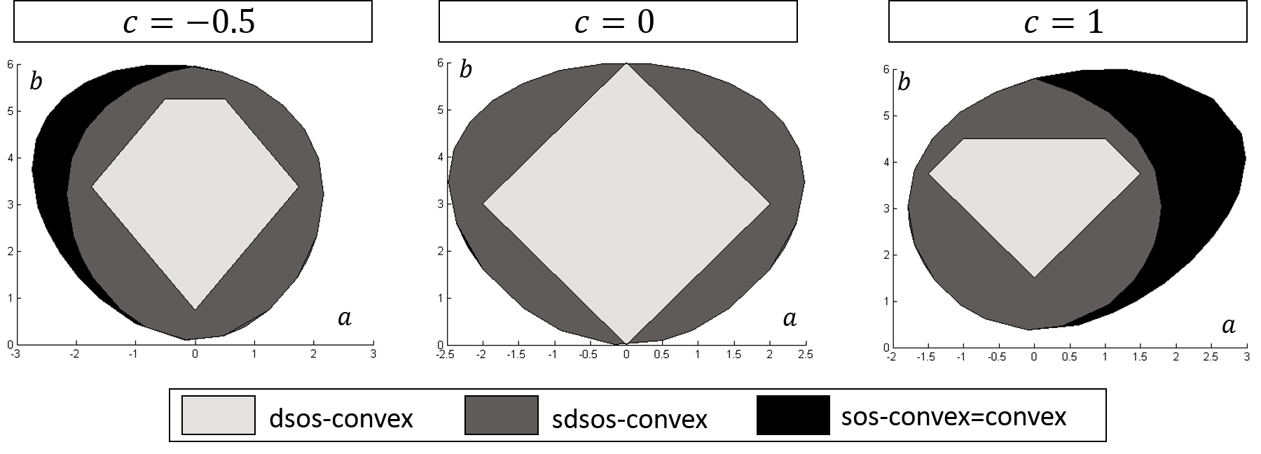
Figure 5.1: The sets $\Sigma_{D}C_{n,2d},\Sigma_{S}C_{n,2d}$ and $\Sigma C_{n,2d}$ for the parametric family of polynomials in (5.13)

5.3.2 Existence of difference of s/d/sos-convex decompositions of polynomials

The reason we introduced the notions of s/d/sos-convexity is that in our optimization problems for finding dcds, we would like to replace the condition

$$f=g-h,~{}g,h\text{ convex}$$

with the computationally tractable condition

$$f=g-h,~{}g,h\text{ s/d/sos-convex.}$$

The first question that needs to be addressed is whether for any polynomial such a decomposition exists. In this section, we prove that this is indeed the case. This in particular implies that a dcd can be found efficiently.

We start by proving a lemma about cones.

Lemma 5.3.4.

Consider a vector space $E$ and a full-dimensional cone $K\subseteq E$. Then, any $v\in E$ can be written as $v=k_{1}-k_{2},$ where $k_{1},k_{2}\in K.$

Proof.

Let $v\in E$. If $v\in K$, then we take $k_{1}=v$ and $k_{2}=0$. Assume now that $v\notin K$ and let $k$ be any element in the interior of the cone $K$. As $k\in int(K)$, there exists $0<\alpha<1$ such that $k^{\prime}\mathrel{\mathop{:}}=(1-\alpha)v+\alpha k\in K.$ Rewriting the previous equation, we obtain

$$v=\frac{1}{1-\alpha}k^{\prime}-\frac{\alpha}{1-\alpha}k.$$

By taking $k_{1}\mathrel{\mathop{:}}=\frac{1}{1-\alpha}k^{\prime}$ and $k_{2}\mathrel{\mathop{:}}=\frac{\alpha}{1-\alpha}k$, we observe that $v=k_{1}-k_{2}$ and $k_{1},k_{2}\in K$. ∎

The following theorem is the main result of the section.

Theorem 5.3.5.

Any polynomal $p\in\tilde{\mathcal{H}}_{n,2d}$ can be written as the difference of two dsos-convex polynomials in $\tilde{\mathcal{H}}_{n,2d}.$

Corollary 5.3.6.

Any polynomial $p\in\tilde{\mathcal{H}}_{n,2d}$ can be written as the difference of two sdsos-convex, sos-convex, or convex polynomials in $\tilde{\mathcal{H}}_{n,2d}$.

Proof.

This is straightforward from the inclusions

$$\tilde{\Sigma}_{D}C_{n,2d}\subseteq\tilde{\Sigma}_{S}C_{n,2d}\subseteq\tilde{\Sigma}C_{n,2d}\subseteq\tilde{C}_{n,2d}.\ \$$

∎

In view of Lemma 5.3.4, it suffices to show that $\tilde{\Sigma}_{D}C_{n,2d}$ is full dimensional in the vector space $\tilde{\mathcal{H}}_{n,2d}$ to prove Theorem 5.3.5. We do this by constructing a polynomial in $int(\tilde{\Sigma}_{D}C_{n,2d})$ for any $n,d$.

Recall that $z_{n,d}$ (resp. $\tilde{z}_{n,d}$) denotes the vector of all monomials in $x=(x_{1},\ldots,x_{n})$ of degree exactly (resp. up to) $d$. If $y=(y_{1},\ldots,y_{n})$ is a vector of variables of length $n$, we define

$$w_{n,d}(x,y)\mathrel{\mathop{:}}=y\cdot z_{n,d}(x),$$

where $y\cdot z_{n,d}(x)=(y_{1}z_{n,d}(x),\ldots,y_{n}z_{n,d}(x))^{T}.$ Analogously, we define

$$\tilde{w}_{n,d}(x,y)\mathrel{\mathop{:}}=y\cdot\tilde{z}_{n,d}(x).$$

Theorem 5.3.7.

For all $n,d$, there exists a polynomial $p\in\tilde{\mathcal{H}}_{n,2d}$ such that

$$y^{T}H_{p}(x)y=\tilde{w}^{T}_{n,d-1}(x,y)Q\tilde{w}_{n,d-1}(x,y),$$ (5.14)

where $Q$ is strictly dd.

Any such polynomial will be in $int(\tilde{\Sigma}_{D}C_{n,2d})$. Indeed, if we were to pertub the coefficients of $p$ slightly, then each coefficient of $Q$ would undergo a slight perturbation. As $Q$ is strictly dd, $Q$ would remain dd, and hence $p$ would remain dsos-convex.

We will prove Theorem 5.3.7 through a series of lemmas. First, we show that this is true in the homogeneous case and when $n=2$ (Lemma 5.3.8). By induction, we prove that this result still holds in the homogeneous case for any $n$ (Lemma 5.3.9). We then extend this result to the nonhomogeneous case.

Lemma 5.3.8.

For all $d$, there exists a polynomial $p\in\tilde{\mathcal{H}}_{2,2d}$ such that

$$y^{T}H_{p}(x)y=w^{T}_{2,d-1}(x,y)Qw_{2,d-1}(x,y),$$ (5.15)

for some strictly dd matrix $Q$.

We remind the reader that Lemma 5.3.8 corresponds to the base case of a proof by induction on $n$ for Theorem 5.3.7.

Proof.

In this proof, we show that there exists a polynomial $p$ that satisfies (5.15) for some strictly dd matrix $Q$ in the case where $n=2$, and for any $d\geq 1.$

First, if $2d=2$, we simply take $p(x_{1},x_{2})=x_{1}^{2}+x_{2}^{2}$ as $y^{T}H_{p}(x)y=2y^{T}Iy$ and the identity matrix is strictly dd. Now, assume $2d>2$. We consider two cases depending on whether $d$ is divisible by $2$.

In the case that it is, we construct $p$ as

$$p(x_{1},x_{2})\mathrel{\mathop{:}}=a_{0}x_{1}^{2d}+a_{1}x_{1}^{2d-2}x_{2}^{2}+a_{2}x_{1}^{2d-4}x_{2}^{4}+\ldots+a_{d/2}x_{1}^{d}x_{2}^{d}+\ldots+a_{1}x_{1}^{2}x_{2}^{2d-2}+a_{0}x_{2}^{2d},$$

with the sequence $\{a_{k}\}_{k=0,\ldots,\frac{d}{2}}$ defined as follows

$$a_{1} =1$$ (5.16)

$$a_{k+1} =\left(\frac{2d-2k}{2k+2}\right)a_{k},~{}k=1,\ldots,\frac{d}{2}-1\text{ (for }2d>4)$$

$$a_{0} =\frac{1}{d}+\frac{d}{2(2d-1)}a_{\frac{d}{2}}.$$

Let

$$\beta_{k} =a_{k}(2d-2k)(2d-2k-1),k=0,\ldots,\frac{d}{2}-1,$$ (5.17)

$$\gamma_{k} =a_{k}\cdot 2k(2k-1),k=1,\ldots,\frac{d}{2},$$

$$\delta_{k} =a_{k}(2d-2k)\cdot 2k,k=1,\ldots,\frac{d}{2}.$$

We claim that the matrix $Q$ defined as

is strictly dd and satisfies (5.15) with $w_{2,d-1}(x,y)$ ordered as

$$\begin{pmatrix}y_{1}x_{1}^{d-1},y_{1}x_{1}^{d-2}x_{2},\ldots,y_{1}x_{1}x_{2}^{d-2},y_{1}x_{2}^{d-1},y_{2}x_{1}^{d-1},y_{2}x_{1}^{d-2}x_{2},\ldots,y_{2}x_{1}x_{2}^{d-2},y_{2}x_{2}^{d-1}\end{pmatrix}^{T}.$$

To show (5.15), one can derive the Hessian of $p$, expand both sides of the equation, and verify equality. To ensure that the matrix is strictly dd, we want all diagonal coefficients to be strictly greater than the sum of the elements on the row. This translates to the following inequalities

$$\beta_{0} >\delta_{1}+\delta_{\frac{d}{2}}$$

$$\beta_{k} >\delta_{k+1},\forall k=1,\ldots,\frac{d}{2}-2$$

$$\beta_{\frac{d}{2}-1} >0,\gamma_{1}>0$$

$$\gamma_{k+1} >\delta_{k},\forall k=1,\ldots,\frac{d}{2}-1.$$

Replacing the expressions of $\beta_{k},\gamma_{k}$ and $\delta_{k}$ in the previous inequalities using (5.17) and the values of $a_{k}$ given in (5.16), one can easily check that these inequalities are satisfied.

We now consider the case where $d$ is not divisable by 2 and take

$$p(x_{1},x_{2})\mathrel{\mathop{:}}=a_{0}x_{1}^{2d}+a_{1}x_{1}^{2d-2}x_{2}^{2}+\ldots+a_{(d-1)/2}x_{1}^{d+1}x_{2}^{d-1}+a_{(d-1)/2}x_{1}^{d-1}x_{2}^{d+1}+\ldots+a_{1}x_{1}^{2}x_{2}^{2d-2}+a_{0}x_{2}^{2d},$$

with the sequence $\{a_{k}\}_{k=0,\ldots,\frac{d-1}{2}}$ defined as follows

$$a_{1} =1$$ (5.18)

$$a_{k+1} =\left(\frac{2d-2k}{2k+2}\right)a_{k},~{}k=1,\ldots,\frac{d-3}{2}$$

$$a_{0} =1+\frac{2(2d-2)}{2d(2d-1)}.$$

Again, we want to show existence of a strictly dd matrix $Q$ that satisfies (5.15). Without changing the definitions of the sequences $\{\beta_{k}\}_{k=1,\ldots,\frac{d-3}{2}}$,$\{\gamma_{k}\}_{k=1,\ldots,\frac{d-1}{2}}$ and $\{\delta_{k}\}_{k=1,\ldots,\frac{d-1}{2}}$, we claim this time that the matrix $Q$ defined as

satisfies (5.15) and is strictly dd. Showing (5.15) amounts to deriving the Hessian of $p$ and checking that the equality is verified. To ensure that $Q$ is strictly dd, the inequalities that now must be verified are

$$\beta_{k} >\delta_{k+1},\forall k=0,\ldots,\frac{d-1}{2}-1$$

$$\gamma_{k} >\delta_{k-1},\forall k=2,\ldots,\frac{d-1}{2}$$

$$\gamma_{1} >0.$$

These inequalities can all be shown to hold using (5.18).

∎

Lemma 5.3.9.

For all $n,d,$ there exists a form $p_{n,2d}\in\mathcal{H}_{n,2d}$ such that

$$y^{T}H_{p_{n,2d}}(x)y=w^{T}_{n,d-1}(x,y)Q_{p_{n,2d}}w_{n,d-1}(x,y)$$

and $Q_{p_{n,2d}}$ is a strictly dd matrix.

Proof.

We proceed by induction on $n$ with fixed and arbitrary $d$. The property is verified for $n=2$ by Lemma 5.3.8. Suppose that there exists a form $p_{n,2d}\in\mathcal{H}_{n,2d}$ such that

$$y^{T}H_{p_{n,2d}}y=w^{T}_{n,d-1}(x,y)Q_{p_{n,2d}}w_{n,d-1}(x,y),$$ (5.19)

for some strictly dd matrix $Q_{p_{n,2d}}.$ We now show that

$$p_{n+1,2d}\mathrel{\mathop{:}}=q+\alpha v$$

with

$$q \mathrel{\mathop{:}}=\sum_{\{i_{1},\ldots,i_{n}\}\in\{1,\ldots,n+1\}^{n}}p_{n,2d}(x_{i_{1}},\ldots,x_{i_{n}})$$ (5.20)

$$v \mathrel{\mathop{:}}=\sum_{2i_{1}+\ldots 2i_{n+1}=2d,i_{1},\ldots,i_{n+1}>0}x_{1}^{2i_{1}}x_{2}^{2i_{2}}\ldots x_{n+1}^{2i_{n+1}},$$

and $\alpha>0$ small enough, verifies

$$y^{T}H_{p_{n+1,2d}}y=w^{T}_{n+1,d-1}(x,y)Q_{p_{n+1,2d}}w_{n+1,d-1}(x,y),$$ (5.21)

for some strictly dd matrix $Q_{p_{n+1,2d}}$. Equation (5.21) will actually be proved using an equivalent formulation that we describe now. Recall that

$$w_{n+1,d-1}(x,y)=y\cdot z_{n+1,d-1},$$

where $z_{n+1,d-1}$ is the standard vector of monomials in $x=(x_{1},\ldots,x_{n+1})$ of degree exactly $d-1$. Let $\hat{w}_{n}$ be a vector containing all monomials from $w_{n+1,d-1}$ that include up to $n$ variables in $x$ and $\hat{w}_{n+1}$ be a vector containing all monomials from $w_{n+1,d-1}$ with exactly $n+1$ variables in $x$. Obviously, $w_{n+1,d-1}$ is equal to

$$\hat{w}\mathrel{\mathop{:}}=\begin{pmatrix}\hat{w}_{n}\\ \hat{w}_{n+1}\end{pmatrix}$$

up to a permutation of its entries. If we show that there exists a strictly dd matrix $\hat{Q}$ such that

$$y^{T}H_{p_{n+1,2d}}(x)y=\hat{w}^{T}(x,y)\hat{Q}\hat{w}(x,y)$$ (5.22)

then one can easily construct a strictly dd matrix $Q_{p_{n+1,2d}}$ such that (5.21) will hold by simply permuting the rows of $\hat{Q}$ appropriately.

We now show the existence of such a $\hat{Q}$. To do this, we claim and prove the following:

• Claim 1: there exists a strictly dd matrix $\hat{Q}_{q}$ such that

  $$y^{T}H_{q}(x)y=\begin{pmatrix}\hat{w}_{n}\\ \hat{w}_{n+1}\end{pmatrix}^{T}\begin{pmatrix}\hat{Q}_{q}&0\\ 0&0\end{pmatrix}\begin{pmatrix}\hat{w}_{n}\\ \hat{w}_{n+1}\end{pmatrix}.$$ (5.23)

• Claim 2: there exist a symmetric matrix $\hat{Q}_{v}$, and $q_{1},\ldots,q_{m}>0$ (where $m$ is the length of $\hat{w}_{n+1}$) such that

  $$y^{T}H_{v}(x)y=\begin{pmatrix}\hat{w}_{n}\\ \hat{w}_{n+1}\end{pmatrix}^{T}\begin{pmatrix}\hat{Q}_{v}&0\\ 0&\text{diag}(q_{1},\ldots,q_{m})\end{pmatrix}\begin{pmatrix}\hat{w}_{n}\\ \hat{w}_{n+1}\end{pmatrix}.$$ (5.24)

Using these two claims and the fact that $p_{n+1,2d}=q+\alpha v$, we get that

$$y^{T}H_{p_{n+1,2d}}(x)y=y^{T}H_{q}(x)y+\alpha y^{T}H_{v}(x)y=\hat{w}^{T}(x,y)\hat{Q}\hat{w}(x,y)$$

where

$$\hat{Q}=\begin{pmatrix}\hat{Q}_{q}+\alpha\hat{Q}_{v}&0\\ 0&\alpha\text{ diag}(q_{1},\ldots,q_{m})\end{pmatrix}.$$

As $\hat{Q}_{q}$ is strictly dd, we can pick $\alpha>0$ small enough such that $\hat{Q}_{q}+\alpha\hat{Q}_{v}$ is strictly dd. This entails that $\hat{Q}$ is strictly dd, and (5.22) holds.

It remains to prove the two claims to be done.

Proof of Claim 1: Claim 1 concerns the polynomial $q$, defined as the sum of polynomials $p_{n,2d}(x_{i_{1}},\ldots,x_{i_{n}})$. Note from (5.19) that the Hessian of each of these polynomials has a strictly dd Gram matrix in the monomial vector $w_{n,d-1}.$ However, the statement of Claim 1 involves the monomial vector $\hat{w}_{n}$. So, we start by linking the two monomial vectors. If we denote by

$$M=\mathop{\cup}_{(i_{1},\ldots,i_{n})\in\{1,\ldots,n+1\}^{n}}\{\text{monomials in }w_{n,d-1}(x_{i_{1}},\ldots,x_{i_{n}},y)\},$$

then $M$ is exactly equal to $\hat{M}=\{\text{monomials in }\hat{w}_{n}(x,y)\}$ as the entries of both are monomials of degree 1 in $y$ and of degree $d-1$ and in $n$ variables of $x=(x_{1},\ldots,x_{n+1}).$

By definition of $q$, we have that

$$y^{T}H_{q}y=\sum_{(i_{1},\ldots,i_{n})\in\{1,\ldots,n+1\}^{n}}w_{n,d-1}(x_{i_{1}},\ldots,x_{i_{n}},y)^{T}Q_{p_{n,2d}(x_{i_{1}},\ldots,x_{i_{n}})}w_{n,d-1}(x_{i_{1}},\ldots,x_{i_{n}},y)$$

We now claim that there exists a strictly dd matrix $\hat{Q}_{q}$ such that

$$y^{T}H_{q}y=\hat{w}_{n}^{T}\hat{Q}_{q}\hat{w}_{n}.$$

This matrix is constructed by padding the strictly dd matrices $Q_{p_{n,2d}(x_{i_{1}},\ldots,x_{i_{n}})}$ with rows of zeros and then adding them up. The sum of two rows that verify the strict diagonal dominance condition still verifies this condition. So we only need to make sure that there is no row in $\hat{Q}_{q}$ that is all zero. This is indeed the case because $\hat{M}\subseteq M.$

Proof of Claim 2: Let $I\mathrel{\mathop{:}}=\{i_{1},\ldots,i_{n}~{}|~{}i_{1}+\ldots+i_{n+1}=d,i_{1},\ldots,i_{n+1}>0\}$ and $\hat{w}_{n+1}^{i}$ be the $i^{th}$ element of $\hat{w}_{n+1}$. To prove (5.24), we need to show that

$$y^{T}H_{v}(x)y=\sum_{i_{1},\ldots,i_{n}\in I}\sum_{k=1}^{n+1}2i_{k}(2i_{k}-1)x_{1}^{2i_{1}}\ldots x_{k}^{2i_{k}-2}\ldots x_{n+1}^{2i_{n+1}}y_{k}^{2}$$ (5.25)

$$+4\sum_{i_{1},\ldots,i_{m}\in I}\sum_{j\neq k}i_{k}i_{j}x_{1}^{2i_{1}}\ldots x_{j}^{2i_{j}-1}\ldots x_{k}^{2i_{k}-1}\ldots x_{n+1}^{2i_{n+1}}y_{j}y_{k}.$$

can equal

$$\hat{w}_{n}^{T}(x,y)\hat{Q}_{v}\hat{w}_{n}^{T}(x,y)+\sum_{i=1}^{m}q_{i}(\hat{w}_{n+1}^{i})^{2}$$ (5.26)

for some symmetric matrix $\hat{Q}_{v}$ and positive scalars $q_{1},\ldots,q_{m}$. We first argue that all monomials contained in $y^{T}H_{v}(x)y$ appear in the expansion (5.26). This means that we do not need to use any other entry of the Gram matrix in (5.24). Since every monomial appearing in the first double sum of (5.25) involves only even powers of variables, it can be obtained via the diagonal entries of $Q_{v}$ together with the entries $q_{1},\ldots,q_{m}.$ Moreover, since the coefficient of each monomial in this double sum is positive and since the sum runs over all possible monomials consisting of even powers in $n+1$ variables, we conclude that $q_{i}>0$, for $i=1,\ldots,m.$

Consider now any monomial contained in the second double sum of (5.25). We claim that any such monomial can be obtained from off-diagonal entries in $\hat{Q}_{v}.$ To prove this claim, we show that it can be written as the product of two monomials $m^{\prime}$ and $m^{\prime\prime}$ with $n$ or fewer variables in $x=(x_{1},\ldots,x_{n+1})$. Indeed, at least two variables in the monomial must have degree less than or equal to $d-1$. Placing one variable in $m^{\prime}$ and the other variable in $m^{\prime\prime}$ and then filling up $m^{\prime}$ and $m^{\prime\prime}$ with the remaining variables (in any fashion as long as the degrees at $m^{\prime}$ and $m^{\prime\prime}$ equal $d-1$) yields the desired result.

∎

of Theorem 5.3.7.

Let $p_{n,2k}\in\mathcal{H}_{n,2k}$ be the form constructed in the proof of Lemma 5.3.9 which is in the interior of $\Sigma_{D}C_{n,2k}.$ Let $Q_{k}$ denote the strictly diagonally dominant matrix which was constructed to satisfy

$$y^{T}H_{p_{n,2k}}y=w_{n,2k}^{T}(x,y)Q_{k}w_{n,2k}.$$

To prove Theorem 5.3.7, we take

$$p\mathop{\mathrel{:}}=\sum_{k=1}^{d}p_{n,2k}\in\tilde{\mathcal{H}}_{n,2d}.$$

We have

$$y^{T}H_{p}(x)y =\begin{pmatrix}w_{n,1}(x,y)\\ \vdots\\ w_{n,d-1}(x,y)\end{pmatrix}^{T}\begin{pmatrix}Q_{1}&&\\ &\ddots&\\ &&Q_{d}\end{pmatrix}\begin{pmatrix}w_{n,1}(x,y)\\ \vdots\\ w_{n,d-1}(x,y)\end{pmatrix}$$

$$=\tilde{w}_{n,d-1}(x,y)^{T}Q\tilde{w}_{n,d-1}(x,y).$$

We observe that $Q$ is strictly dd, which shows that $p\in int(\tilde{\Sigma}_{D}C_{n,2d}).$ ∎

Remark 5.3.10.

If we had only been interested in showing that any polynomial in $\tilde{\mathcal{H}}_{n,2d}$ could be written as a difference of two sos-convex polynomials, this could have been easily done by showing that $p(x)=\left(\sum_{i}x_{i}^{2}\right)^{d}\in int(\Sigma C_{n,2d})$. However, this form is not dsos-convex or sdsos-convex for all $n,d$ (e.g., for $n=3$ and $2d=8$). We have been unable to find a simpler proof for existence of sdsos-convex dcds that does not go through the proof of existence of dsos-convex dcds.

Remark 5.3.11.

If we solve problem (5.6) with the convexity constraint replaced by a dsos-convexity (resp. sdsos-convexity, sos-convexity) requirement, the same arguments used in the proof of Theorem 5.2.6 now imply that the optimal solution $g^{*}$ is not dominated by any dsos-convex (resp. sdsos-convex, sos-convex) decomposition.

5.4 Numerical results

In this section, we present a few numerical results to show how our algebraic decomposition techniques affect the convex-concave procedure. The objective function $p\in\tilde{\mathcal{H}}_{n,2d}$ in all of our experiments is generated randomly following the ensemble of [155, Section 5.1.]. This means that

$$p(x_{1},\ldots,x_{n})=\sum_{i=1}^{n}x_{i}^{2d}+g(x_{1},\ldots,x_{n}),$$

where $g$ is a random polynomial of total degree $\leq 2d-1$ whose coefficients are random integers uniformly sampled from $[-30,30].$ An advantage of polynomials generated in this fashion is that they are bounded below and that their minimum $p^{*}$ is achieved over $\mathbb{R}^{n}.$ We have intentionally restricted ourselves to polynomials of degree equal to $4$ in our experiments as this corresponds to the smallest degree for which the problem of finding a dc decomposition of $f$ is hard, without being too computationally expensive. Experimenting with higher degrees however would be a worthwhile pursuit in future work. The starting point of CCP was generated randomly from a zero-mean Gaussian distribution.

One nice feature of our decomposition techniques is that all the polynomials $f_{i}^{k},i=0,\ldots,m$ in line 4 of Algorithm 1 in the introduction are sos-convex. This allows us to solve the convex subroutine of CCP exactly via a single SDP [53, Remark 3.4.], [110, Corollary 2.3.]:

$$\min\gamma$$ (5.27)

$$\text{s.t. }f_{0}^{k}-\gamma=\sigma_{0}+\sum_{j=1}^{m}\lambda_{j}f_{j}^{k}$$

$$\sigma_{0}\text{ sos},~{}\lambda_{j}\geq 0,j=1,\ldots,m.$$

The degree of $\sigma_{0}$ here is taken to be the maximum degree of $f_{0}^{k},\ldots,f_{m}^{k}$. We could have also solved these subproblems using standard descent algorithms for convex optimization. However, we are not so concerned with the method used to solve this convex problem as it is the same for all experiments. All of our numerical examples were done using MATLAB, the polynomial optimization library SPOT [137], and the solver MOSEK [140].

5.4.1 Picking a good dc decomposition for CCP

In this subsection, we consider the problem of minimizing a random polynomial $f_{0}\in\tilde{\mathcal{H}}_{8,4}$ over a ball of radius $R$, where $R$ is a random integer in $[20,50].$ The goal is to compare the impact of the dc decomposition of the objective on the performance of CCP. To monitor this, we decompose the objective in 4 different ways and then run CCP using the resulting decompositions. These decompositions are obtained through different SDPs that are listed in Table 5.1.

Feasibility	$\lambda_{\max}H_{h}(x_{0})$	$\lambda_{\max,B}H_{h}$	Undominated
	$\min t$	$\min_{g,h}t$
$\min 0$	$\text{s.t. }f_{0}=g-h,$	$\text{s.t. }f_{0}=g-h,$	$\min\frac{1}{\mathcal{A}_{n}}\int\mbox{Tr}H_{g}d\sigma$
$\text{s.t. }f_{0}=g-h,$	$g,h$ sos-convex	$g,h$ sos-convex	$\text{s.t. }f_{0}=g-h,$
$g,h$ sos-convex	$tI-H_{h}(x_{0})\succeq 0$	$y^{T}(tI-H_{h}(x)+f_{1}\tau(x))y$ sos	$g,h$ sos-convex
		$y^{T}\tau(x)y$ sos

Table 5.1: Different decomposition techniques using sos optimization

The first SDP in Table 5.1 is simply a feasibility problem. The second SDP minimizes the largest eigenvalue of $H_{h}$ at the initial point $x_{0}$ inputed to CCP. The third minimizes the largest eigenvalue of $H_{h}$ over the ball $B$ of radius $R$. Indeed, let $f_{1}\mathrel{\mathop{:}}=\sum_{i}x_{i}^{2}-R^{2}.$ Notice that $\tau(x)\succeq 0,\forall x$ and if $x\in B$, then $f_{1}(x)\leq 0$. This implies that $tI\succeq H_{h}(x),\forall x\in B.$ The fourth SDP searches for an undominated dcd.

Once $f_{0}$ has been decomposed, we start CCP. After $4$ mins of total runtime, the program is stopped and we recover the objective value of the last iteration. This procedure is repeated on 30 random instances of $f_{0}$ and $R$, and the average of the results is presented in Figure 5.2.

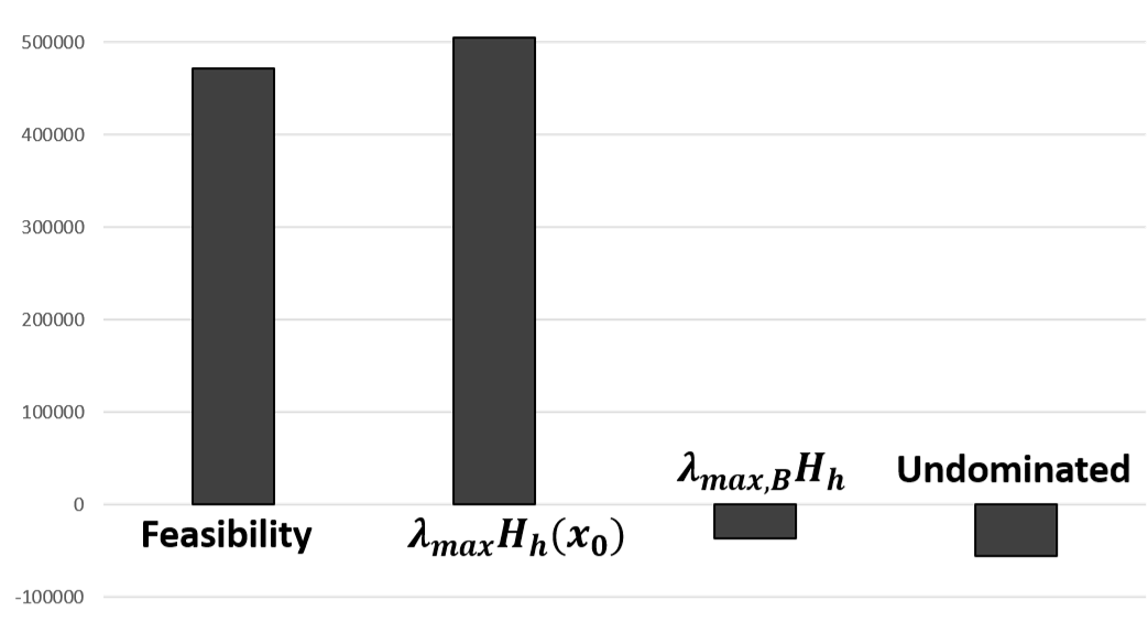
Figure 5.2: Impact of choosing a good dcd on CCP ($n=8,2d=4$)

From the figure, we can see that the choice of the initial decomposition impacts the performance of CCP considerably, with the region formulation of $\lambda_{\max}$ and the undominated decomposition giving much better results than the other two. It is worth noting that all formulations have gone through roughly the same number of iterations of CCP (approx. 400). Furthermore, these results seem to confirm that it is best to pick an undominated decomposition when applying CCP.

5.4.2 Scalibility of s/d/sos-convex dcds and the multiple decomposition CCP

While solving the last optimization problem in Table 5.1 usually gives very good results, it relies on an sos-convex dc decomposition. However, this choice is only reasonable in cases where the number of variables and the degree of the polynomial that we want to decompose are low. When these become too high, obtaining an sos-convex dcd can be too time-consuming. The concepts of dsos-convexity and sdsos-convexity then become interesting alternatives to sos-convexity. This is illustrated in Table 5.2, where we have reported the time taken to solve the following decomposition problem:

$$\min\frac{1}{\mathcal{A}_{n}}\int_{S^{n-1}}\mbox{Tr }H_{g}d\sigma$$ (5.28)

$$\text{s.t. }f=g-h,g,h\text{ s/d/sos-convex}$$

In this case, $f$ is a random polynomial of degree $4$ in $n$ variables. We also report the optimal value of (5.28) (we know that (5.28) is always guaranteed to be feasible from Theorem 5.3.7).

	n=6		n=10		n=14		n=18
	Time	Value	Time	Value	Time	Value	Time	Value
dsos-convex	$<1s$	62090	$<$1s	168481	2.33s	136427	6.91s	48457
sdsos-convex	$<1s$	53557	1.11 s	132376	3.89s	99667	12.16s	32875
sos-convex	$<1s$	11602	44.42s	18346	800.16s	9828	30hrs+	——

Table 5.2: Time and optimal value obtained when solving (5.28)

Notice that for $n=18$, it takes over 30 hours to obtain an sos-convex decomposition, whereas the run times for s/dsos-convex decompositions are still in the range of 10 seconds. This increased speed comes at a price, namely the quality of the decomposition. For example, when $n=10$, the optimal value obtained using sos-convexity is nearly 10 times lower than that of sdsos-convexity.

Now that we have a better quantitative understanding of this tradeoff, we propose a modification to CCP that leverages the speed of s/dsos-convex dcds for large $n$. The idea is to modify CCP in such a way that one would compute a new s/dsos-convex decomposition of the functions $f_{i}$ after each iteration. Instead of looking for dcds that would provide good global decompositions (such as undominated sos-convex dcds), we look for decompositions that perform well locally. From Section 5.2, candidate decomposition techniques for this task can come from formulations (5.4) and (5.5) that minimize the maximum eigenvalue of the Hessian of $h$ at a point or the trace of the Hessian of $h$ at a point. This modified version of CCP is described in detail in Algorithm 2. We will refer to it as multiple decomposition CCP.

We compare the performance of CCP and multiple decomposition CCP on the problem of minimizing a polynomial $f$ of degree 4 in $n$ variables, for varying values of $n$. In Figure 5.3, we present the optimal value (averaged over 30 instances) obtained after 4 mins of total runtime. The “SDSOS” columns correspond to multiple decomposition CCP (Algorithm 2) with sdsos-convex decompositions at each iteration. The “SOS” columns correspond to classical CCP where the first and only decomposition is an undominated sos-convex dcd. From Figure 5.2, we know that this formulation performs well for small values of $n$. This is still the case here for $n=8$ and $n=10$. However, this approach performs poorly for $n=12$ as the time taken to compute the initial decomposition is too long. In contrast, multiple decomposition CCP combined with sdsos-convex decompositions does slightly worse for $n=8$ and $n=10$, but significantly better for $n=12$.

Algorithm 2 Multiple decomposition CCP ($\lambda_{\max}$ version)

1:$x_{0},~{}f_{i},i=0,\ldots,m$

2:$k\leftarrow 0$

3:while stopping criterion not satisfied do

4:     Decompose: $\forall i$ find $g_{i}^{k},h_{i}^{k}$ s/d/sos-convex that min. $t$, s.t. $tI-H_{h_{i}^{k}}(x_{k})$ s/ddand $f_{i}=g_{i}^{k}-h_{i}^{k}$

5:     Convexify: $f_{i}^{k}(x)\mathrel{\mathop{:}}=g_{i}^{k}(x)-(h_{i}^{k}(x_{k})+\nabla h_{i}^{k}(x_{k})^{T}(x-x_{k})),~{}i=0,\ldots,m$

6:     Solve convex subroutine: $\min f_{0}^{k}(x)$, s.t. $f_{i}^{k}(x)\leq 0,i=1,\ldots,m$

7:     $x_{k+1}\mathrel{\mathop{:}}=\underset{f_{i}^{k}(x)\leq 0}{\text{argmin}}f_{0}^{k}(x)$

8:     $k\leftarrow k+1$

9:end while

10:$x_{k}$

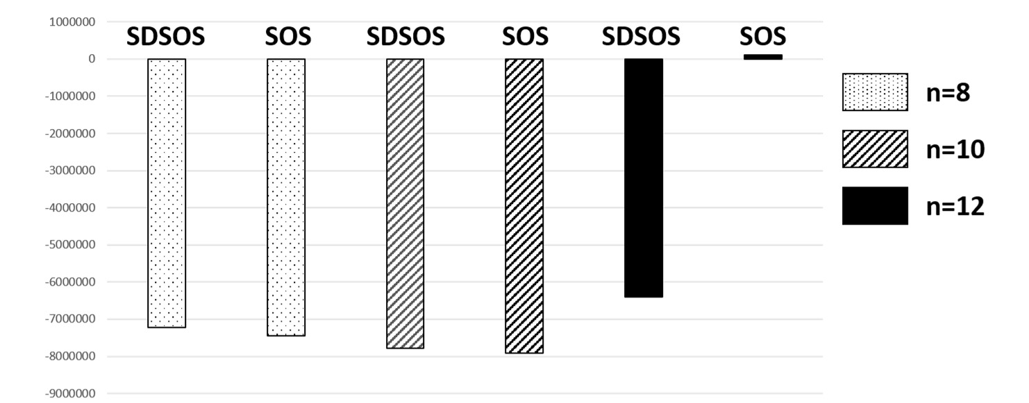
Figure 5.3: Comparing multiple decomposition CCP using sdsos-convex decompositions against CCP with a single undominated sos-convex decomposition

In conclusion, our overall observation is that picking a good dc decomposition noticeably affects the perfomance of CCP. While optimizing over all dc decompositions is intractable for polynomials of degree greater or equal to $4$, the algebraic notions of sos-convexity, sdsos-convexity and dsos-convexity can provide valuable relaxations. The choice among these options depends on the number of variables and the degree of the polynomial at hand. Though these classes of polynomials only constitute subsets of the set of convex polynomials, we have shown that even the smallest subset of the three contains dcds for any polynomial.

Chapter 6 Polynomials Norms

6.1 Introduction

A function $f:\mathbb{R}^{n}\rightarrow\mathbb{R}$ is a norm if it satisfies the following three properties:

1. positive definiteness: $f(x)>0,~{}\forall x\neq 0,$ and $f(0)=0$.

2. $1$-homogeneity: $f(\lambda x)=|\lambda|f(x),~{}\forall x\in\mathbb{R}^{n},~{}\forall\lambda\in\mathbb{R}$.

3. triangle inequality: $f(x+y)\leq f(x)+f(y),~{}\forall x,y\in\mathbb{R}^{n}.$

Some well-known examples of norms include the $1$-norm, $f(x)=\sum_{i=1}^{n}|x_{i}|$, the $2$-norm, $f(x)=\sqrt{\sum_{i=1}^{n}x_{i}^{2}}$, and the $\infty$-norm, $f(x)=\max_{i}|x_{i}|.$ Our focus throughout this chapter is on norms that can be derived from multivariate polynomials. More specifically, we are interested in establishing conditions under which the $d^{th}$ root of a homogeneous polynomial of degree $d$ is a norm, where $d$ is an even number. We refer to the norm obtained when these conditions are met as a polynomial norm. It is easy to see why we restrict ourselves to $d^{th}$ roots of degree-$d$ homogeneous polynomials. Indeed, nonhomogeneous polynomials cannot hope to satisfy the homogeneity condition and homogeneous polynomials of degree $d>1$ are not 1-homogeneous unless we take their $d^{th}$ root. The question of when the square root of a homogeneous quadratic polynomial is a norm (i.e., when $d=2$) has a well-known answer (see, e.g., [35, Appendix A]): a function $f(x)=\sqrt{x^{T}Qx}$ is a norm if and only if the symmetric $n\times n$ matrix $Q$ is positive definite. In the particular case where $Q$ is the identity matrix, one recovers the $2$-norm. Positive definiteness of $Q$ can be checked in polynomial time using for example Sylvester’s criterion (positivity of the $n$ leading principal minors of $Q$). This means that testing whether the square root of a quadratic form is a norm can be done in polynomial time. A similar characterization in terms of conditions on the coefficients are not known for polynomial norms generated by forms of degree greater than 2. In particular, it is not known whether one can efficiently test membership or optimize over the set of polynomial norms.

Outline and contributions.

In this chapter, we study polynomial norms from a computational perspective. In Section 6.2, we give two different necessary and sufficient conditions under which the $d^{th}$ root of a degree-$d$ form $f$ will be a polynomial norm: namely, that $f$ be strictly convex (Theorem 6.2.2), or (equivalently) that $f$ be convex and postive definite (Theorem 6.2.1). Section 6.3 investigates the relationship between general norms and polynomial norms: while many norms are polynomial norms (including all $p$-norms with $p$ even), some norms are not (consider, e.g., the $1$-norm). We show, however, that any norm can be approximated to arbitrary precision by a polynomial norm (Theorem 6.3.1). In Section 6.4, we move on to complexity results and show that simply testing whether the $4^{th}$ root of a quartic form is a norm is strongly NP-hard (Theorem 6.4.1). We then provide a semidefinite programming-based test for checking whether the $d^{th}$ root of a degree $d$ form is a norm (Theorem 6.4.4) and a semidefinite programming-based hierarchy to optimize over a subset of the set of polynomial norms (Theorem 6.4.20). The latter is done by introducing the concept of $r$-sum of squares-convexity (see Definition 6.4.6). We show that any form with a positive definite Hessian is $r$-sos-convex for some value of $r$, and present a lower bound on that value (Theorem 6.4.7). We also show that the level $r$ of the semidefinite programming hierarchy cannot be bounded as a function of the number of variables and the degree only (Theorem 6.4.18). Finally, we cover a few applications of polynomial norms in statistics and dynamical systems in Section 6.5. In Section 6.5.1, we compute approximations of two different types of norms, polytopic gauge norms and $p$-norms with $p$ noneven, using polynomial norms. The techniques described in this section can be applied to norm regression. In Section 6.5.2, we use polynomial norms to prove stability of a switched linear system, a task which is equivalent to computing an upperbound on the joint spectral radius of a family of matrices.

6.2 Two equivalent characterizations of polynomial norms

We start this section with two theorems that provide conditions under which the $d^{th}$ root of a degree-$d$ form is a norm. These will be useful in Section 6.4 to establish semidefinite programming-based approximations of polynomial norms. Note that throughout this chapter, $d$ is taken to be an even positive integer.

Theorem 6.2.1.

The $d^{th}$ root of a degree-$d$ form $f$ is a norm if and only if $f$ is convex and positive definite.

Proof.

If $f^{1/d}$ is a norm, then $f^{1/d}$ is positive definite, and so is $f$. Furthermore, any norm is convex and the $d^{th}$ power of a nonnegative convex function remains convex.

Assume now that $f$ is convex and positive definite. We show that $f^{1/d}$ is a norm. Positivity and homogeneity are immediate. It remains to prove the triangle inequality. Let $g\mathrel{\mathop{:}}=f^{1/d}$. Denote by $S_{f}$ and $S_{g}$ the 1-sublevel sets of $f$ and $g$ respectively. It is clear that

$$S_{g}=\{x~{}|~{}f^{1/d}(x)\leq 1\}=\{x~{}|~{}f(x)\leq 1\}=S_{f},$$

and as $f$ is convex, $S_{f}$ is convex and so is $S_{g}$. Let $x,y\in\mathbb{R}^{n}.$ We have that $\frac{x}{g(x)}\in S_{g}$ and $\frac{y}{g(y)}\in S_{g}$. From convexity of $S_{g}$,

$$g\left(\frac{g(x)}{g(x)+g(y)}\cdot\frac{x}{g(x)}+\frac{g(y)}{g(x)+g(y)}\cdot\frac{y}{g(y)}\right)\leq 1.$$

Homogeneity of $g$ then gives us

$$\frac{1}{g(x)+g(y)}g(x+y)\leq 1$$

which shows that triangle inequality holds. ∎

Theorem 6.2.2.

The $d^{th}$ root of a degree-$d$ form $f$ is a norm if and only if $f$ is strictly convex, i.e.,

$$f(\lambda x+(1-\lambda)y)<\lambda f(x)+(1-\lambda)f(y),~{}\forall x\neq y,~{}\forall\lambda\in(0,1).$$

Proof.

We will show that a degree-d form $f$ is strictly convex if and only $f$ is convex and positive definite. The result will then follow from Theorem 6.2.1.

Suppose $f$ is strictly convex, then the first-order characterization of strict convexity gives us that

$$f(y)>f(x)+\nabla f(x)^{T}(y-x),~{}\forall y\neq x.$$

For $x=0$, the inequality becomes $f(y)>0,~{}\forall y\neq 0$, as $f(0)=0$ and $\nabla f(0)=0$. Hence, $f$ is positive definite. Of course, a strictly convex function is also convex.

Suppose now that $f$ is convex, positive definite, but not strictly convex, i.e., there exists $\bar{x},\bar{y}\in\mathbb{R}^{n}$ with $\bar{x}\neq\bar{y}$, and $\gamma\in(0,1)$ such that

$$f\left(\gamma\bar{x}+(1-\gamma)\bar{y}\right)=\gamma f(\bar{x})+(1-\gamma)f(\bar{y}).$$

Let $g(\alpha)\mathrel{\mathop{:}}=f(\bar{x}+\alpha(\bar{y}-\bar{x})).$ Note that $g$ is a restriction of $f$ to a line and, consequently, $g$ is a convex, positive definite, univariate polynomial in $\alpha$. We now define

$$h(\alpha)\mathrel{\mathop{:}}=g(\alpha)-(g(1)-g(0))\alpha-g(0).$$ (6.1)

Similarly to $g$, $h$ is a convex univariate polynomial as it is the sum of two convex univariate polynomials. We also know that $h(\alpha)\geq 0,\forall\alpha\in(0,1)$. Indeed, by convexity of $g$, we have that $g(\alpha x+(1-\alpha)y)\geq\alpha g(x)+(1-\alpha)g(y),\forall x,y\in\mathbb{R}$ and $\alpha\in(0,1)$. This inequality holds in particular for $x=1$ and $y=0$, which proves the claim. Observe now that $h(0)=h(1)=0$. By convexity of $h$ and its nonnegativity over $(0,1)$, we have that $h(\alpha)=0$ on $(0,1)$ which further implies that $h=0$. Hence, from (6.1), $g$ is an affine function. As $g$ is positive definite, it cannot be that $g$ has a nonzero slope, so $g$ has to be a constant. But this contradicts that $\lim_{\alpha\rightarrow\infty}g(\alpha)=\infty.$ To see why this limit must be infinite, we show that $\lim_{||x||\rightarrow\infty}f(x)=\infty.$ As $\lim_{\alpha\rightarrow\infty}||\bar{x}+\alpha(\bar{y}-\bar{x})||=\infty$ and $g(\alpha)=f(\bar{x}+\alpha(\bar{y}-\bar{x}))$, this implies that $\lim_{\alpha\rightarrow\infty}g(\alpha)=\infty.$ To show that $\lim_{||x||\rightarrow\infty}f(x)=\infty$, let

$$x^{*}=\underset{||x||=1}{\text{argmin }}f(x).$$

By positive definiteness of $f$, $f(x^{*})>0.$ Let $M$ be any positive scalar and define $R\mathrel{\mathop{:}}=(M/f(x^{*}))^{1/d}$. Then for any $x$ such that $||x||=R$, we have

$$f(x)\geq\min_{||x||=R}f(x)\geq R^{d}f(x^{*})=M,$$

where the second inequality holds by homogeneity of $f.$ Thus $\lim_{||x||\rightarrow\infty}f(x)=\infty$. ∎

6.3 Approximating norms by polynomial norms

It is easy to see that not all norms are polynomial norms. For example, the 1-norm $||x||_{1}=\sum_{i=1}^{n}|x_{i}|$ is not a polynomial norm. Indeed, all polynomial norms are differentiable at all but one point (the origin) whereas the 1-norm is nondifferentiable whenever one of the components of $x$ is equal to zero. In this section, we show that, though not every norm is a polynomial norm, any norm can be approximated to arbitrary precision by a polynomial norm (Theorem 6.3.1). The proof of this theorem is inspired from a proof by Ahmadi and Jungers in [3, 6]. A related result is given by Barvinok in [24]. In that chapter, he shows that any norm can be approximated by the $d$-th root of a nonnegative degree-$d$ form, and quantifies the quality of the approximation as a function of $n$ and $d$. The form he obtains however is not shown to be convex. In fact, in a later work [25, Section 2.4], Barvinok points out that it would be an interesting question to know whether any norm can be approximated by the $d^{th}$ root of a convex form with the same quality of approximation as for $d$-th roots of nonnegative forms. The result below is a step in that direction though no quantitative result on the quality of approximation is given. Throughout, $S^{n-1}$ denotes the unit sphere in $\mathbb{R}^{n}.$

Theorem 6.3.1.

Let $||\cdot||$ be any norm on $\mathbb{R}^{n}.$ For any $\epsilon>0$, there exist an even integer $d$ and a convex positive definite form $f$ of degree $d$ such that

$$\max_{x\in S^{n-1}}|~{}f^{1/d}(x)-||x||~{}|\leq\epsilon.$$

Note that, from Theorem 6.2.1, $f^{1/d}$ is a polynomial norm as $f$ is a convex positive definite form. To show this result, we start with the following lemma.

Lemma 6.3.2.

Let $||\cdot||$ be any norm on $\mathbb{R}^{n}$. For any $\epsilon>0$, there exist an even integer $d$ and an $n$-variate convex positive definite form $f$ of degree $d$ such that

$$||x||\leq f^{1/d}(x)\leq(1+\epsilon)||x||,~{}\forall x\in\mathbb{R}^{n}.$$ (6.2)

Proof.

Throughout, we let $B_{\alpha}\mathrel{\mathop{:}}=\{x~{}|~{}||x||\leq\alpha\}.$ When $\alpha=1$, we drop the subscript and simply denote by $B$ the unit ball of $||\cdot||$. We will also use the notation $\partial S$ to denote the boundary of a set $S$ and $int(S)$ to denote its interior. Let $\bar{\epsilon}\mathrel{\mathop{:}}=\frac{\epsilon}{1+\epsilon}$. The crux of the proof lies in proving that there exists an integer $d$ and a positive definite convex form $f$ of degree $d$ such that

$$B_{1-\bar{\epsilon}}\subseteq\{x~{}|~{}f(x)\leq 1\}\subseteq B.$$ (6.3)

If we prove this, then Lemma 6.3.2 can be obtained as follows. Let $x\in\mathbb{R}^{n}.$ To show the first inequality in (6.2), we proceed by contradiction. Suppose that $||x||>f^{1/d}(x)$. If $f^{1/d}(x)\neq 0$, then $||x/f^{1/d}(x)||>1$ while $f(x/f^{1/d}(x))=1$. (If $f^{1/d}(x)=0$ then $x=0$ and the inequality holds.) Hence,

$$x/f^{1/d}(x)\in\{x~{}|~{}f(x)\leq 1\}$$

but $x/f^{1/d}(x)\notin B$ which contradicts (6.3). To prove the second inequality in (6.2), note that the first inclusion of $(\ref{eq:level.set.incl})$ gives us $f^{1/d}((1-\bar{\epsilon})x/||x||)\leq 1$, which is equivalent to $f^{1/d}(x/||x||)\leq\frac{1}{1-\bar{\epsilon}}=1+\epsilon.$ Multiplying by $||x||$ on both sides gives us the result.

We now focus on showing the existence of a positive definite convex form $f$ that satisfies (6.3). The proof is a simplification of the proof of Theorem 3.2. in [3, 6] with some modifications.

Let $x\in\partial B_{1-\bar{\epsilon}/2}$. To any such $x$, we associate a dual vector $v(x)$ orthogonal to a supporting hyperplane of $B_{1-\bar{\epsilon}/2}$ at $x$. By definition of a supporting hyperplane, we have that $v(x)^{T}y\leq v(x)^{T}x$, $\forall y\in B_{1-\bar{\epsilon}/2}$, and, as $B_{1-\bar{\epsilon}}\subset B_{1-\bar{\epsilon}/2}$, we have

$$v(x)^{T}y<v(x)^{T}x,\forall y\in B_{1-\bar{\epsilon}}.$$ (6.4)

Let

$$S(x)\mathrel{\mathop{:}}=\{y~{}|~{}v(x)^{T}y>v(x)^{T}x\text{ and }||y||=1\}.$$

It is easy to see that $S(x)$ is an open subset of the boundary $\partial B$ of $B$. Futhermore, since $x\in int(B)$, $x/||x||\in S(x)$ which implies that $S(x)$ is nonempty and that the family of sets $S(x)$ (as $x$ ranges over $\partial B_{1-\bar{\epsilon}/2})$ is a covering of $\partial B$. As $\{S(x)\}_{x\in\partial B_{1-\bar{\epsilon}/2}}$ is an open covering of the compact set $\partial B$, there exists a finite covering of $\partial B$, i.e., one can choose $x_{1},\ldots,x_{N}\in\partial B_{1-\bar{\epsilon}/2}$ in such a way that $\cup_{i=1}^{N}S(x_{i})=\partial B.$

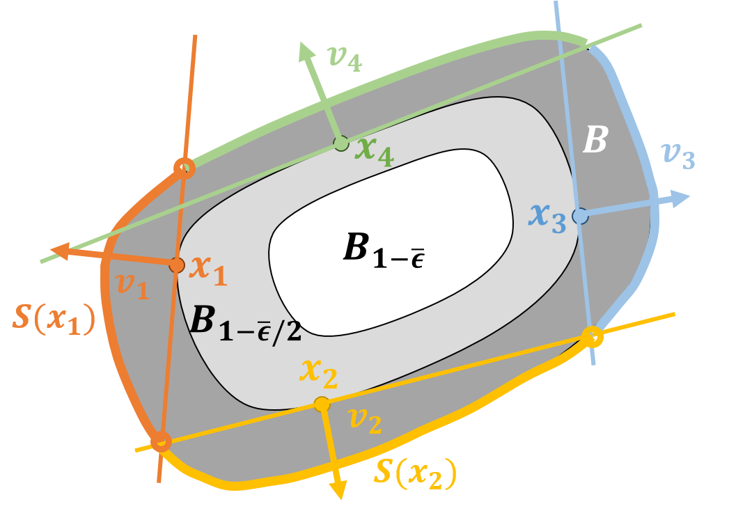
Figure 6.1: An illustration of the construction of the open covering of $\partial B$.

For ease of notation, we now let $v_{i}\mathrel{\mathop{:}}=v(x_{i})$ for all $i=1,\ldots,N$. From (6.4), we have that $\frac{v_{i}^{T}y}{v_{i}^{T}x_{i}}<1$ for any $i$ and for any $y\in B_{1-\bar{\epsilon}}$. Since $B_{1-\bar{\epsilon}}$ is compact, we get $\max_{i}\max_{y\in B_{1-\bar{\epsilon}}}\left(\frac{v_{i}^{T}y}{v_{i}^{T}x_{i}}\right)<1$. Hence, there exists an integer $d$ such that

$$\left(\max_{i}\max_{y\in B_{1-\bar{\epsilon}}}\left(\frac{v_{i}^{T}y}{v_{i}^{T}x_{i}}\right)\right)^{d}<\frac{1}{N}.$$ (6.5)

We now define

$$f(y)\mathrel{\mathop{:}}=\sum_{i=1}^{N}\left(\frac{v_{i}^{T}y}{v_{i}^{T}x_{i}}\right)^{d},$$ (6.6)

where $d$ is any integer satisfying (6.5). The form $f$ is convex as a sum of even powers of linear forms. Let

$$\mathcal{L}\mathrel{\mathop{:}}=\{y~{}|~{}f(y)\leq 1\}.$$

By (6.5), it is straightforward to see that $B_{1-\bar{\epsilon}}\subseteq\mathcal{L}.$

We now show that $\mathcal{L}\subseteq int(B).$ Let $y\in\mathcal{L}$, then $f(y)\leq 1.$ If a sum of nonnegative terms is less than or equal to 1, then each term has to be less than or equal to $1$, which implies that $\frac{v_{i}^{T}y}{v_{i}^{T}x_{i}}\leq 1$, for all $i=1,\ldots,N.$ From this, we deduce that $y\notin\partial B$. Indeed, if $y\in\partial B$, there exists $i\in\{1,\ldots,N\}$ such that $y\in S(x_{i})$ as $\{S(x_{i})\}_{i}$ is a cover of $\partial B$. But, by definition of $S(x_{i})$, we would have $v_{i}^{T}y>v_{i}^{T}x_{i}$ which contradicts the previous statement. We have that $\partial B\cap\mathcal{L}=\emptyset$ as a consequence. However, as $\mathcal{L}$ and $B$ both contain the zero vector, this implies that $\mathcal{L}\subseteq int(B).$ Note that the previous inclusion guarantees positive definiteness of $f$. Indeed, if $f$ were not positive definite, $\mathcal{L}$ would be unbounded and could not be a subset of $B$ (which is bounded). ∎

Proof of Theorem 6.3.1.

Let $\epsilon>0$ and denote by $\alpha\mathrel{\mathop{:}}=\max_{x\in S^{n-1}}||x||$. By Lemma 6.3.2, there exists an integer $d$ and a convex form $f$ such that

$$||x||\leq f^{1/d}(x)\leq\left(1+\frac{\epsilon}{\alpha}\right)||x||,~{}\forall x.$$

This is equivalent to

$$0\leq f^{1/d}(x)-||x||\leq\frac{\epsilon}{\alpha}||x||,\forall x.$$

For $x\in S^{n-1}$, as $||x||/\alpha\leq 1$, this inequality becomes

$$0\leq f^{1/d}(x)-||x||\leq\epsilon.$$

∎

Remark 6.3.3.

We remark that the polynomial norm constructed in Theorem 6.3.1 is the $d^{th}$-root of an sos-convex polynomial. Hence, one can approximate any norm on $\mathbb{R}^{n}$ by searching for a polynomial norm using semidefinite programming. To see why the polynomial $f$ in (6.6) is sos-convex, observe that linear forms are sos-convex and that an even power of an sos-convex form is sos-convex.

6.4 Semidefinite programming-based approximations of polynomial norms

6.4.1 Complexity

It is natural to ask whether testing if the $d^{th}$ root of a given degree-$d$ form is a norm can be done in polynomial time. In the next theorem, we show that, unless $P=NP$, this is not the case even when $d=4$.

Theorem 6.4.1.

Deciding whether the $4^{th}$ root of a quartic form is a norm is strongly NP-hard.

Proof.

The proof of this result is adapted from a proof in [10]. Recall that the CLIQUE problem can be described thus: given a graph $G=(V,E)$ and a positive integer $k$, decide whether $G$ contains a clique of size at least $k$. The CLIQUE problem is known to be NP-hard [71]. We will give a reduction from CLIQUE to the problem of testing convexity and positive definiteness of a quartic form. The result then follows from Theorem 6.2.1. Let $\omega(G)$ be the clique number of the graph at hand, i.e., the number of vertices in a maximum clique of $G$. Consider the following quartic form

$$b(x;y)\mathrel{\mathop{:}}=-2k\sum_{i,j\in E}x_{i}x_{j}y_{i}y_{j}-(1-k)\left(\sum_{i}x_{i}^{2}\right)\left(\sum_{i}y_{i}^{2}\right).$$

In [10], using in part a result in [122], it is shown that

$$\omega(G)\leq k\Leftrightarrow b(x;y)+\frac{n^{2}\gamma}{2}\left(\sum_{i=1}^{n}x_{i}^{4}+\sum_{i=1}^{n}y_{i}^{4}+\sum_{1\leq i<j\leq n}(x_{i}^{2}x_{j}^{2}+y_{i}^{2}y_{j}^{2})\right)$$ (6.7)

is convex and $b(x;y)$ is positive semidefinite. Here, $\gamma$ is a positive constant defined as the largest coefficient in absolute value of any monomial present in some entry of the matrix $\left[\frac{\partial^{2}b(x;y)}{\partial x_{i}\partial y_{j}}\right]_{i,j}$. As $\sum_{i}x_{i}^{4}+\sum_{i}y_{i}^{4}$ is positive definite and as we are adding this term to a positive semidefinite expression, the resulting polynomial is positive definite. Hence, the equivalence holds if and only if the quartic on the righthandside of the equivalence in (6.7) is convex and positive definite. ∎

Note that this also shows that strict convexity is hard to test for quartic forms (this is a consequence of Theorem 6.2.2). A related result is Proposition 3.5. in [10], which shows that testing strict convexity of a polynomial of even degree $d\geq 4$ is hard. However, this result is not shown there for forms, hence the relevance of the previous theorem.

Theorem 6.4.1 motivates the study of tractable sufficient conditions to be a polynomial norm. The sufficient conditions we consider next are based on semidefinite programming.

6.4.2 Sum of squares polynomials and semidefinite programming review

We start this section by reviewing the notion of sum of squares polynomials and related concepts such as sum of squares-convexity. We say that a polynomial $f$ is a sum of squares (sos) if $f(x)=\sum_{i}q_{i}^{2}(x)$, for some polynomials $q_{i}$. Being a sum of squares is a sufficient condition for being nonnegative. The converse however is not true, as is exemplified by the Motzkin polynomial

$$M(x,y)=x^{4}y^{2}+x^{2}y^{4}−3x^{2}y^{2}+1$$ (6.8)

which is nonnegative but not a sum of squares [141]. The sum of squares condition is a popular surrogate for nonnegativity due to its tractability. Indeed, while testing nonnegativity of a polynomial of degree greater or equal to 4 is a hard problem, testing whether a polynomial is a sum of squares can be done using semidefinite programming. This comes from the fact that a polynomial $p$ of degree $d$ is a sum of squares if and only if there exists a positive semidefinite matrix $Q$ such that $f(x)=z(x)^{T}Qz(x)$, where $z(x)$ is the standard vector of monomials of degree up to $d$ (see, e.g., [152]). As a consequence, any optimization problem over the coefficients of a set of polynomials which includes a combination of affine constraints and sos constraints on these polynomials, together with a linear objective can be recast as a semidefinite program. These type of optimization problems are known as sos programs.

Though not all nonnegative polynomials can be written as sums of squares, the following theorem by Artin [18] circumvents this problem using sos multipliers.

Theorem 6.4.2 (Artin [18]).

For any nonnegative polynomial $f$, there exists an sos polynomial $q$ such that $q\cdot f$ is sos.

This theorem in particular implies that if we are given a polynomial $f$, then we can always check its nonnegativity using an sos program that searches for $q$ (of a fixed degree). However, the condition does not allow us to optimize over the set of nonnegative polynomials using an sos program (as far as we know). This is because, in that setting, products of decision varibles arise from multiplying polymomials $f$ and $q$, whose coefficients are decision variables.

By adding further assumptions on $f$, Reznick showed in [164] that one could further pick $q$ to be a power of $\sum_{i}x_{i}^{2}$.

Theorem 6.4.3 (Reznick [164]).

Let $f$ be a positive definite form of degree $d$ in $n$ variables and define

$$\epsilon(f)\mathrel{\mathop{:}}=\frac{\min\{f(u)~{}|~{}u\in S^{n-1}\}}{\max\{f(u)~{}|~{}u\in S^{n-1}\}}.$$

If $r\geq\frac{nd(d-1)}{4\log(2)\epsilon(f)}-\frac{n+d}{2}$, then $(\sum_{i=1}^{n}x_{i}^{2})^{r}\cdot f$ is a sum of squares.

Motivated by this theorem, the notion of $r$-sos polynomials can be defined: a polynomial $f$ is said to be $r$-sos if $(\sum_{i}x_{i}^{2})^{r}\cdot f$ is sos. Note that it is clear that any $r$-sos polynomial is nonnegative and that the set of $r$-sos polynomials is included in the set of $(r+1)$-sos polynomials. The Motzkin polynomial in (6.8) for example is $1$-sos although not sos.

To end our review, we briefly touch upon the concept of sum of squares-convexity (sos-convexity), which we will build upon in the rest of the section. Let $H_{f}$ denote the Hessian matrix of a polynomial $f$. We say that $f$ is sos-convex if $y^{T}H_{f}(x)y$ is a sum of squares (as a polynomial in $x$ and $y$). As before, optimizing over the set of sos-convex polynomials can be cast as a semidefinite program. Sum of squares-convexity is obviously a sufficient condition for convexity via the second-order characterization of convexity. However, there are convex polynomials which are not sos-convex (see, e.g., [11]). For a more detailed overview of sos-convexity including equivalent characterizations and settings in which sos-convexity and convexity are equivalent, refer to [12].

Notation

Throughout, we will use the notation $H_{n,d}$ (resp. $P_{n,d}$) to denote the set of forms (resp. positive semidefinite, aka nonnegative, forms) in $n$ variables and of degree $d$. We will futhermore use the falling factorial notation $(t)_{0}=1$ and $(t)_{k}=t(t-1)\ldots(t-(k-1))$ for a positive integer $k$.

6.4.3 A test for validity of polynomial norms

In this subsection, we assume that we are given a form $f$ of degree $d$ and we would like to test whether $f^{1/d}$ is a norm using semidefinite programming.

Theorem 6.4.4.

Let $f$ be a degree-$d$ form. Then $f^{1/d}$ is a polynomial norm if and only if there exist $c>0$, $r\in\mathbb{N}$, and an sos form $q(x,y)$ such that $q(x,y)\cdot y^{T}H_{f}(x,y)y$ is sos and $\left(f(x)-c(\sum_{i}x_{i}^{2})^{d/2}\right)(\sum_{i}x_{i}^{2})^{r}$ is sos. Furthermore, this condition can be checked using semidefinite programming.

Proof.

It is immediate to see that if there exist such a $c$, $r$, and $q$, then $f$ is convex and positive definite. From Theorem 6.2.1, this means that $f^{1/d}$ is a polynomial norm.

Conversely, if $f^{1/d}$ is a polynomial norm, then, by Theorem 6.2.1, $f$ is convex and positive definite. As $f$ is convex, the polynomial $y^{T}H_{f}(x)y$ is nonnegative. Using Theorem 6.4.2, we conclude that there exists an sos polynomial $q(x,y)$ such that $q(x,y)\cdot y^{T}H_{f}(x)y$ is sos. We now show that, as $f$ is positive definite, there exist $c>0$ and $r\in\mathbb{N}$ such that $\left(f(x)-c(\sum_{i}x_{i}^{2})^{d/2}\right)(\sum_{i}x_{i}^{2})^{r}$ is sos. Let $f_{min}$ denote the minimum of $f$ on the sphere. As $f$ is positive definite, $f_{min}>0.$ We take $c\mathrel{\mathop{:}}=\frac{f_{min}}{2}$ and consider $g(x)\mathrel{\mathop{:}}=f(x)-c(\sum_{i}x_{i}^{2})^{d/2}$. We have that $g$ is a positive definite form: indeed, if $x$ is a nonzero vector in $\mathbb{R}^{n}$, then

$$\frac{g(x)}{||x||^{d}}=\frac{f(x)}{||x||^{d}}-c=f\left(\frac{x}{||x||}\right)-c>0,$$

by homogeneity of $f$ and definition of $c$. Using Theorem 6.4.3, $\exists r\in\mathbb{N}$ such that $g(x)(\sum_{i}x_{i}^{2})^{r}$ is sos.

For fixed $r$, a given form $f$, and a fixed degree $d$, one can search for $c>0$ and an sos form $q$ of degree $d$ such that $q(x,y)\cdot y^{T}H_{f}(x,y)y$ is sos and $\left(f(x)-c(\sum_{i}x_{i}^{2})^{d/2}\right)(\sum_{i}x_{i}^{2})^{r}$ is sos using semidefinite programming. This is done by solving the following semidefinite feasibility problem:

$$q(x,y)\text{ sos}$$ (6.9)

$$c\geq 0$$

$$q(x,y)\cdot y^{T}H_{f}(x,y)y\text{ sos}$$

$$\left(f(x)-c\left(\sum_{i}x_{i}^{2}\right)^{d/2}\right)\left(\sum_{i}x_{i}^{2}\right)^{r}\text{ sos},$$

where the unknowns are the coefficients of $q$ and the real number $c$. ∎

Remark 6.4.5.

We remark that we are not imposing $c>0$ in the semidefinite program above. This is because, in practice, especially if the semidefinite program is solved with interior point methods, the solution returned by the solver will be in the interior of the feasible set, and hence $c$ will automatically be positive. One can slightly modify (6.9) however to take the constraint $c>0$ into consideration explicitely. Indeed, consider the following semidefinite feasibility problem where both the degree of $q$ and the integer $r$ are fixed:

$$q(x,y)\text{ sos}$$

$$\gamma\geq 0$$

$$q(x,y)\cdot y^{T}H_{f}(x,y)y\text{ sos}$$

$$\left(\gamma f(x)-\left(\sum_{i}x_{i}^{2}\right)^{d/2}\right)\left(\sum_{i}x_{i}^{2}\right)^{r}\text{ sos}.$$ (6.10)

It is easy to check that (6.10) is feasible with $\gamma\geq 0$ if and only if the last constraint of (6.9) is feasible with $c>0$. To see this, take $c=1/\gamma$ and note that $\gamma$ can never be zero.

To the best of our knowledge, we cannot use the approach described in Theorem 6.4.4 to optimize over the set of polynomial norms with a semidefinite program. This is because of the product of decision variables in the coefficients of $f$ and $q$. The next subsection will address this issue.

6.4.4 Optimizing over the set of polynomial norms

In this subsection, we consider the problem of optimizing over the set of polynomial norms. To do this, we introduce the concept of $r$-sos-convexity. Recall that the notation $H_{f}$ references the Hessian matrix of a form $f$.

Positive definite biforms and r-sos-convexity

Definition 6.4.6.

For an integer $r$, we say that a polynomial $f$ is $r$-sos-convex if $y^{T}H_{f}(x)y\cdot(\sum_{i}x_{i}^{2})^{r}$ is sos.

Observe that, for fixed $r$, the property of $r$-sos-convexity can be checked using semidefinite programming (though the size of this SDP gets larger as $r$ increases). Any polynomial that is $r$-sos-convex is convex. Note that the set of $r$-sos-convex polynomials is a subset of the set of $(r+1)$-sos-convex polynomials and that the case $r=0$ corresponds to the set of sos-convex polynomials.

It is natural to ask whether any convex polynomial is $r$-sos-convex for some $r$. Our next theorem shows that this is the case under a mild assumption.

Theorem 6.4.7.

Let $f$ be a form of degree $d$ such that $y^{T}H_{f}(x)y>0$ for $(x,y)\in S^{n-1}\times S^{n-1}$. Let

$$\eta(f)\mathrel{\mathop{:}}=\frac{\min\{y^{T}H_{f}(x)y~{}|~{}(x,y)\in S^{n-1}\times S^{n-1}\}}{\max\{y^{T}H_{f}(x)y~{}|~{}(x,y)\in S^{n-1}\times S^{n-1}\}}.$$

If $r\geq\frac{n(d-2)(d-3)}{4\log(2)\eta(f)}-\frac{n+d-2}{2}-d$, then $f$ is $r$-sos-convex.

Remark 6.4.8.

Note that $\eta(f)$ can also be interpreted as

$$\eta(f)=\frac{\min_{x\in S^{n-1}}\lambda_{\min}(H_{f}(x))}{\max_{x\in S^{n-1}}\lambda_{\max}(H_{f}(x))}=\frac{1}{\max_{x\in S^{n-1}}\|H^{-1}_{f}(x)\|_{2}\cdot\max_{x\in S^{n-1}}\|H_{f}(x)\|_{2}}.$$

Remark 6.4.9.

Theorem 6.4.7 is a generalization of Theorem 6.4.3 by Reznick. Note though that this is not an immediate generalization. First, $y^{T}H_{f}(x)y$ is not a positive definite form (consider, e.g., $y=0$ and any nonzero $x$). Secondly, note that the multiplier is $(\sum_{i}x_{i}^{2})^{r}$ and does not involve the $y$ variables. (As we will see in the proof, this is essentially because $y^{T}H_{f}(x)y$ is quadratic in $y$.)

Remark 6.4.10.

Theorem 6.4.7 can easily be adapted to biforms of the type $\sum_{j}f_{j}(x)g_{j}(y)$ where $f_{j}$’s are forms of degree $d$ in $x$ and $g_{j}$’s are forms of degree $\tilde{d}$ in $y$. In this case, there exist integers $s,r$ such that

$$\sum_{j}f_{j}(x)g_{j}(y)\cdot(\sum_{i}x_{i}^{2})^{r}\cdot(\sum_{i}y_{i}^{2})^{s}$$

is sos. For the purposes of this chapter however and the connection to polynomial norms, we will show the result in the particular case where the biform of interest is $y^{T}H_{f}(x)y.$

We associate to any form $f\in H_{n,d}$, the $d$-th order differential operator $f(D)$, defined by replacing each occurence of $x_{j}$ with $\frac{\partial}{\partial x_{j}}$. For example, if $f(x_{1},\ldots,x_{n})\mathrel{\mathop{:}}=\sum_{i}c_{i}x_{1}^{a_{1}^{i}}\ldots x_{n}^{a_{i}^{n}}$ where $c_{i}\in\mathbb{R}$ and $a_{j}^{i}\in\mathbb{N}$, then its differential operator will be

$$f(D)=\sum_{i}c_{i}\frac{\partial^{a_{1}^{i}}}{\partial x_{1}^{a_{1}^{i}}}\ldots\frac{\partial^{a_{n}^{i}}}{\partial x_{n}^{a_{n}^{i}}}.$$

Our proof will follow the structure of the proof of Theorem 6.4.3 given in [164] and reutilize some of the results given in the chapter which we quote here for clarity of exposition.

Proposition 6.4.11 ([164], see Proposition 2.6).

For any nonnegative integer $r$, there exist nonnegative rationals $\lambda_{k}$ and integers $\alpha_{kl}$ such that

$$(x_{1}^{2}+\ldots+x_{n}^{2})^{r}=\sum_{k}\lambda_{k}(\alpha_{k1}x_{1}+\ldots+\alpha_{kn}x_{n})^{2r}.$$

For simplicity of notation, we will let $\alpha_{k}\mathrel{\mathop{:}}=(\alpha_{k1},\ldots,\alpha_{kl})^{T}$ and $x\mathrel{\mathop{:}}=(x_{1},\ldots,x_{n})^{T}$. Hence, we will write $\sum_{k}\lambda_{k}(\alpha_{k}^{T}x)^{2r}$ to mean $\sum_{k}\lambda_{k}(a_{k1}x_{1}+\ldots+a_{kn}x_{n})^{2r}$.

Proposition 6.4.12 ([164], see Proposition 2.8).

If $g\in H_{n,e}$ and $h=\sum_{k}\lambda_{k}(\alpha_{k}^{T}x)^{d+e}\in H_{n,d+e}$, then

$$g(D)h=(d+e)_{e}\sum_{k}\lambda_{k}g(\alpha_{k})(\alpha_{k}^{T}x)^{d}.$$

Proposition 6.4.13 ([164], see Theorem 3.7 and 3.9).

For $f\in H_{n,d}$ and $s\geq d$, we define $\Phi_{s}(f)\in H_{n,d}$ by

$$f(D)(x_{1}^{2}+\ldots+x_{n}^{2})^{s}=\mathrel{\mathop{:}}\Phi_{s}(f)(x_{1}^{2}+\ldots+x_{n}^{2})^{s-d}.$$ (6.11)

The inverse $\Phi_{s}^{-1}(f)$ of $\Phi_{s}(f)$ exists and this is a map verifying $\Phi_{s}(\Phi_{s}^{-1}(f))=f.$

Proposition 6.4.14 ([164], see Theorem 3.12 ).

Suppose $f$ is a positive definite form in $n$ variables and of degree $d$ and let

$$\epsilon(f)=\frac{\min\{f(u)~{}|~{}u\in S^{n-1}\}}{\max\{f(u)~{}|~{}u\in S^{n-1}\}}.$$

If $s\geq\frac{nd(d-1)}{4\log(2)\epsilon(f)}-\frac{n-d}{2}$, then $\Phi^{-1}_{s}(f)\in P_{n,d}.$

We will focus throughout the proof on biforms of the following structure

$$F(x;y)\mathrel{\mathop{:}}=\sum_{1\leq i,j\leq n}y_{i}y_{j}p_{ij}(x),$$ (6.12)

where $p_{ij}(x)\in H_{n,d}$, for all $i,j$, and some even integer $d$. Note that the polynomial $y^{T}H_{f}(x)y$ (where $f$ is some form) has this structure. We next present three lemmas which we will then build on to give the proof of Theorem 6.4.7.

Lemma 6.4.15.

For a biform $F(x;y)$ of the structure in (6.12), define the operator $F(D;y)$ as

$$F(D;y)=\sum_{ij}y_{i}y_{j}p_{ij}(D).$$

If $F(x;y)$ is positive semidefinite (i.e., $F(x;y)\geq 0,~{}\forall x,y$), then, for any $s\geq 0$, the biform

$$F(D;y)(x_{1}^{2}+\ldots+x_{n}^{2})^{s}$$

is a sum of squares.

Proof.

Using Proposition 6.4.11, we have

$$(x_{1}^{2}+\ldots+x_{n}^{2})^{s}=\sum_{l}\lambda_{l}(\alpha_{l1}x_{1}+\ldots\alpha_{ln}x_{n})^{2s},$$

where $\lambda_{l}\geq 0$ and $\alpha_{l}\in\mathbb{Z}^{n}.$ Hence, applying Proposition 6.4.12, we get

$$F(D;y)(x_{1}^{2}+\ldots+x_{n}^{2})^{s} =\sum_{i,j}y_{i}y_{j}(p_{ij}(D)(x_{1}^{2}+\ldots+x_{n}^{2})^{s})$$

$$=\sum_{i,j}y_{i}y_{j}\left((2s)_{d}\sum_{l}\lambda_{l}p_{ij}(\alpha_{l})(\alpha_{l}^{T}x)^{2s-d}\right)$$

$$=(2s)_{d}\sum_{l}\lambda_{l}(\alpha_{l}^{T}x)^{2s-d}\sum_{i,j}y_{i}y_{j}p_{ij}(\alpha_{l}).$$ (6.13)

Notice that $\sum_{i,j}y_{i}y_{j}p_{ij}(\alpha_{l})$ is a quadratic form in $y$ which is positive semidefinite by assumption, which implies that it is a sum of squares (as a polynomial in $y$). Furthermore, as $\lambda_{l}\geq 0~{}\forall l$ and $(\alpha_{l}^{T}x)^{2s-d}$ is an even power of a linear form, we have that $\lambda_{l}(\alpha_{l}^{T}x)^{2s-d}$ is a sum of squares (as a polynomial in $x$). Combining both results, we get that (6.13) is a sum of squares. ∎

We now extend the concept introduced by Reznick in Proposition 6.4.13 to biforms.

Lemma 6.4.16.

For a biform $F(x;y)$ of the structure as in (6.12), we define the biform $\Psi_{s,x}(F(x;y))$ as

$$\Psi_{s,x}(F(x;y))\mathrel{\mathop{:}}=\sum_{i,j}y_{i}y_{j}\Phi_{s}(p_{ij}(x)),$$

where $\Phi_{s}$ is as in (6.11). Define

$$\Psi_{s,x}^{-1}(F(x;y))\mathrel{\mathop{:}}=\sum_{i,j}y_{i}y_{j}\Phi_{s}^{-1}(p_{ij}(x)),$$

where $\Phi_{s}^{-1}$ is the inverse of $\Phi_{s}$. Then, we have

$$F(D;y)(x_{1}^{2}+\ldots+x_{n}^{2})^{s}=\Psi_{s,x}(F)(x_{1}^{2}+\ldots+x_{n}^{2})^{s-d}$$ (6.14)

and

$$\Psi_{s,x}(\Psi_{s,x}^{-1}(F))=F.$$ (6.15)

Proof.

We start by showing that (6.14) holds:

$$F(D;y)(x_{1}^{2}+\ldots+x_{n}^{2})^{s} =\sum_{i,j}y_{i}y_{j}p_{ij}(D)(x_{1}^{2}+\ldots+x_{n}^{2})^{s}$$

$$\underset{\text{using (\ref{eq:def.Phi})}}{=}\sum_{i,j}y_{i}y_{j}\Phi_{s}(p_{ij}(x))(x_{1}^{2}+\ldots x_{n}^{2})^{s-d}$$

$$=\Psi_{s,x}(F)(x_{1}^{2}+\ldots+x_{n}^{2})^{s-d}.$$

We now show that (6.15) holds:

$$\Psi_{s,x}(\Psi_{s,x}^{-1}(F))=\Psi_{s,x}\left(\sum_{i,j}y_{i}y_{j}\Phi_{s}^{-1}(p_{ij}(x))\right)=\sum_{i,j}y_{i}y_{j}\Phi_{s}\Phi_{s}^{-1}(p_{ij})=\sum_{i,j}y_{i}y_{j}p_{ij}=F.$$

∎

Lemma 6.4.17.

For a biform $F(x;y)$ of the structure in (6.12), which is positive on the bisphere, let

$$\eta(F)\mathrel{\mathop{:}}=\frac{\min\{F(x;y)~{}|~{}(x,y)\in S^{n-1}\times S^{n-1}\}}{\max\{F(x;y)~{}|~{}(x,y)\in S^{n-1}\times S^{n-1}\}}.$$

If $s\geq\frac{nd(d-1)}{4\log(2)\eta(F)}-\frac{n-d}{2}$, then $\Psi_{s,x}^{-1}(F)$ is positive semidefinite.

Proof.

Fix $y\in S^{n-1}$ and consider $F_{y}(x)=F(x;y)$, which is a positive definite form in $x$ of degree $d$. From Proposition 6.4.14, if

$$s\geq\frac{nd(d-1)}{4\log(2)\epsilon(F_{y})}-\frac{n-d}{2},$$

then $\Phi^{-1}_{s}(F_{y})$ is positive semidefinite. As $\eta(F)\leq\epsilon(F_{y})$ for any $y\in S^{n-1}$, we have that if

$$s\geq\frac{nd(d-1)}{4\log(2)\eta(F)}-\frac{n-d}{2},$$

then $\Phi_{s}^{-1}(F_{y})$ is positive semidefinite, regardless of the choice of $y.$ Hence, $\Psi_{s,x}^{-1}(F)$ is positive semidefinite (as a function of $x$ and $y$).

∎

Proof of Theorem 6.4.7.

Let $F(x;y)=y^{T}H_{f}(x)y$, let $r\geq\frac{n(d-2)(d-3)}{4\log(2)\eta(f)}-\frac{n+d-2}{2}-d$, and let

$$G(x;y)=\Psi_{r+d,x}^{-1}(F).$$

We know by Lemma 6.4.17 that $G(x;y)$ is positive semidefinite. Hence, using Lemma 6.4.15, we get that

$$G(D,y)(x_{1}^{2}+\ldots+x_{n}^{2})^{r+d}$$

is sos. Lemma 6.4.16 then gives us:

$$G(D;y)(x_{1}^{2}+\ldots+x_{n}^{2})^{r+d} \underset{\text{using }(\ref{eq:def.Phi.s.x})}{=}\Psi_{r+d,x}(G)(x_{1}^{2}+\ldots+x_{n}^{2})^{r}$$

$$\underset{\text{using }(\ref{eq:Phi.s.x.inv})}{=}F(x;y)(x_{1}^{2}+\ldots+x_{n}^{2})^{r}.$$

As a consequence, $F(x;y)(x_{1}^{2}+\ldots+x_{n}^{2})^{r}$ is sos.

∎

The last theorem of this section shows that one cannot bound the integer $r$ in Theorem 6.4.7 as a function of $n$ and $d$ only.

Theorem 6.4.18.

For any integer $r\geq 0$, there exists a form $f$ in 3 variables and of degree 8 such that $H_{f}(x)\succ 0,\forall x\neq 0$, but $f$ is not $r$-sos-convex.

Proof.

Consider the trivariate octic:

$$f(x_{1},x_{2},x_{3}) =32x_{1}^{8}+118x_{1}^{6}x_{2}^{2}+40x_{1}^{6}x_{3}^{2}+25x_{1}^{4}x_{2}^{2}x_{3}^{2}-35x_{1}^{4}x_{3}^{4}+3x_{1}^{2}x_{2}^{4}x_{3}^{2}-16x_{1}^{2}x_{2}^{2}x_{3}^{4}+24x_{1}^{2}x_{3}^{6}$$

$$+16x_{2}^{8}+44x_{2}^{6}x_{3}^{2}+70x_{2}^{4}x_{3}^{4}+60x_{2}^{2}x_{3}^{6}+30x_{3}^{8}.$$

It is shown in [11] that $f$ has positive definite Hessian, and that the $(1,1)$ entry of $H_{f}(x)$, which we will denote by $H_{f}^{(1,1)}(x)$, is 1-sos but not sos. We will show that for any $r\in\mathbb{N}$, one can find $s\in\mathbb{N}\backslash\{0\}$ such that

$$g_{s}(x_{1},x_{2},x_{3})=f(x_{1},sx_{2},sx_{3})$$

satisfies the conditions of the theorem.

We start by showing that for any $s$, $g_{s}$ has positive definite Hessian. To see this, note that for any $(x_{1},x_{2},x_{3})\neq 0,(y_{1},y_{2},y_{3})\neq 0$, we have:

$$(y_{1},y_{2},y_{3})H_{g_{s}}(x_{1},x_{2},x_{3})(y_{1},y_{2},y_{3})^{T}=(y_{1},sy_{2},sy_{3})H_{f}(x_{1},sx_{2},sx_{3})(y_{1},sy_{2},sy_{3})^{T}.$$

As $y^{T}H_{f}(x)y>0$ for any $x\neq 0,y\neq 0$, this is in particular true when $x=(x_{1},sx_{2},sx_{3})$ and when $y=(y_{1},sy_{2},sy_{3})$, which gives us that the Hessian of $g_{s}$ is positive definite for any $s\in\mathbb{N}\backslash\{0\}.$

We now show that for a given $r\in\mathbb{N}$, there exists $s\in\mathbb{N}$ such that $(x_{1}^{2}+x_{2}^{2}+x_{3}^{2})^{r}y^{T}H_{g_{s}}(x)y$ is not sos. We use the following result from [166, Theorem 1]: for any positive semidefinite form $p$ which is not sos, and any $r\in\mathbb{N}$, there exists $s\in\mathbb{N}\backslash\{0\}$ such that $(\sum_{i=1}^{n}x_{i}^{2})^{r}\cdot p(x_{1},sx_{2},\ldots,sx_{n})$ is not sos. As $H_{f}^{(1,1)}(x)$ is 1-sos but not sos, we can apply the previous result. Hence, there exists a positive integer $s$ such that

$$(x_{1}^{2}+x_{2}^{2}+x_{3}^{2})^{r}\cdot H_{f}^{(1,1)}(x_{1},sx_{2},sx_{3})=(x_{1}^{2}+x_{2}^{2}+x_{3}^{2})^{r}\cdot H_{g_{s}}^{(1,1)}(x_{1},x_{2},x_{3})$$

is not sos. This implies that $(x_{1}^{2}+x_{2}^{2}+x_{3}^{2})^{r}\cdot y^{T}H_{g_{s}}(x)y$ is not sos. Indeed, if $(x_{1}^{2}+x_{2}^{2}+x_{3}^{2})^{r}\cdot y^{T}H_{g_{s}}(x)y$ was sos, then $(x_{1}^{2}+x_{2}^{2}+x_{3}^{2})^{r}\cdot y^{T}H_{g_{s}}(x)y$ would be sos with $y=(1,0,0)^{T}.$ But, we have

$$(x_{1}^{2}+x_{2}^{2}+x_{3}^{2})^{r}\cdot(1,0,0)H_{g_{s}}(x)(1,0,0)^{T}=(x_{1}^{2}+x_{2}^{2}+x_{3}^{2})^{r}\cdot H_{g_{s}}^{(1,1)}(x),$$

which is not sos. Hence, $(x_{1}^{2}+x_{2}^{2}+x_{3}^{2})^{r}\cdot y^{T}H_{g_{s}}(x)y$ is not sos, and $g$ is not $r$-sos-convex. ∎

Remark 6.4.19.

Any form $f$ with $H_{f}(x)\succ 0,\forall x\neq 0$ is strictly convex but the converse is not true.

To see this, note that any form $f$ of degree $d$ with a positive definite Hessian is convex (as $H_{f}(x)\succeq 0,\forall x$) and positive definite (as, from a recursive application of Euler’s theorem on homogeneous functions, $f(x)=\frac{1}{d(d-1)}x^{T}H_{f}(x)x$). From the proof of Theorem 6.2.2, this implies that $f$ is strictly convex.

To see that the converse statement is not true, consider the strictly convex form $f(x_{1},x_{2})\mathrel{\mathop{:}}=x_{1}^{4}+x_{2}^{4}$. We have

$$H_{f}(x)=12\cdot\begin{bmatrix}x_{1}^{2}&0\\ 0&x_{2}^{2}\end{bmatrix}$$

which is not positive definite e.g., when $x=(1,0)^{T}$.

Optimizing over a subset of polynomial norms with $r$-sos-convexity

In the following theorem, we show how one can efficiently optimize over the set of forms $f$ with $H_{f}(x)\succ 0$, $\forall x\neq 0.$ Comparatively to Theorem 6.4.4, this theorem allows us to impose as a constraint that the $d^{th}$ root of a form be a norm, rather than simply testing whether it is. This comes at a cost however: in view of Remark 6.4.19 and Theorem 6.2.2, we are no longer considering all polynomial norms, but a subset of them whose $d^{th}$ power has a positive definite Hessian.

Theorem 6.4.20.

Let $f$ be a degree-$d$ form. Then $H_{f}(x)\succ 0,\forall x\neq 0$ if and only if $\exists c>0,r\in\mathbb{N}$ such that $f(x)-c(\sum_{i}x_{i}^{2})^{d/2}$ is $r$-sos-convex. Furthermore, this condition can be imposed using semidefinite programming.

Proof.

If there exist $c>0,r\in\mathbb{N}$ such that $g(x)=f(x)-c(\sum_{i}x_{i}^{2})^{d/2}$ is $r$-sos-convex, then $y^{T}H_{g}(x)y\geq 0$, $\forall x,y.$ As the Hessian of $(\sum_{i}x_{i}^{2})^{d/2}$ is positive definite for any nonzero $x$ and as $c>0$, we get $H_{f}(x)\succ 0$, $\forall x\neq 0.$

Conversely, if $H_{f}(x)\succ 0$, $\forall x\neq 0$, then $y^{T}H_{f}(x)y>0$ on the bisphere (and conversely). Let

$$f_{\min}\mathrel{\mathop{:}}=\min_{||x||=||y||=1}y^{T}H_{f}(x)y.$$

We know that $f_{\min}$ is attained and is positive. Take $c\mathrel{\mathop{:}}=\frac{f_{\min}}{2d(d-1)}$ and consider

$$g(x)\mathrel{\mathop{:}}=f(x)-c(\sum_{i}x_{i}^{2})^{d/2}.$$

Then

$$y^{T}H_{g}(x)y=y^{T}H_{f}(x)y-c\cdot\left(d(d-2)(\sum_{i}x_{i}^{2})^{d/2-2}(\sum_{i}x_{i}y_{i})^{2}+d\sum_{i}(x_{i}^{2})^{d/2-1}(\sum_{i}y_{i}^{2})\right).$$

Note that, by Cauchy-Schwarz, we have $(\sum_{i}x_{i}y_{i})^{2}\leq||x||^{2}||y||^{2}$. If $||x||=||y||=1$, we get

$$y^{T}H_{g}(x)y\geq y^{T}H_{f}(x)y-c(d(d-1))>0.$$

Hence, $H_{g}(x)\succ 0,\forall x\neq 0$ and there exists $r$ such that $g$ is $r$-sos-convex from Theorem 6.4.7.

For fixed $r$, the condition that there be $c>0$ such that $f(x)-c(\sum_{i}x_{i}^{2})^{d/2}$ is $r$-sos-convex can be imposed using semidefinite programming. This is done by searching for coefficients of a polynomial $f$ and a real number $c$ such that

$$y^{T}H_{f-c(\sum_{i}x_{i}^{2})^{d/2}}y\cdot(\sum_{i}x_{i}^{2})^{r}\text{ sos}$$ (6.16)

$$c\geq 0.$$

Note that both of these conditions can be imposed using semidefinite programming. ∎

Remark 6.4.21.

Note that we are not imposing $c>0$ in the above semidefinite program. As mentioned in Section 6.4.3, this is because in practice the solution returned by interior point solvers will be in the interior of the feasible set.

In the special case where $f$ is completely free (i.e., when there are no additional affine conditions on the coefficients of $f$), one can take $c\geq 1$ in (6.16) instead of $c\geq 0$. Indeed, if there exists $c>0$, an integer $r$, and a polynomial $f$ such that $f-c(\sum_{i}x_{i}^{2})^{d/2}$ is $r$-sos-convex, then $\frac{1}{c}f$ will be a solution to (6.16) with $c\geq 1$ replacing $c\geq 0$.

6.5 Applications

6.5.1 Norm approximation and regression

In this section, we study the problem of approximating a (non-polynomial) norm by a polynomial norm. We consider two different types of norms: $p$-norms with $p$ noneven (and greater than 1) and gauge norms with a polytopic unit ball. For $p$-norms, we use as an example $||(x_{1},x_{2})^{T}||=(|x_{1}|^{7.5}+|x_{2}|^{7.5})^{1/7.5}$. For our polytopic gauge norm, we randomly generate an origin-symmetric polytope and produce a norm whose 1-sublevel corresponds to that polytope. This allows us to determine the value of the norm at any other point by homogeneity (see [35, Exercise 3.34] for more information on gauge norms, i.e., norms defined by convex, full-dimensional, origin-symmetric sets). To obtain our approximations, we proceed in the same way in both cases. We first sample $N=200$ points $x_{1},\ldots,x_{N}$ on the sphere $S$ that we denote by $x_{1},\ldots,x_{N}$. We then solve the following optimization problem with $d$ fixed:

$$\min_{f\in H_{2,d}} \sum_{i=1}^{N}(||x_{i}||^{d}-f(x_{i}))^{2}$$ (6.17)

s.t. $$f\text{ sos-convex}.$$

Problem (6.17) can be written as a semidefinite program as the objective is a convex quadratic in the coefficients of $f$ and the constraint has a semidefinite representation as discussed in Section 6.4.2. The solution $f$ returned is guaranteed to be convex. Moreover, any sos-convex form is sos (see [89, Lemma 8]), which implies that $f$ is nonnegative. One can numerically check to see if the optimal polynomial is in fact positive definite (for example, by checking the eigenvalues of the Gram matrix of a sum of squares decomposition of $f$). If that is the case, then, by Theorem 6.2.1, $f^{1/d}$ is a norm. Futhermore, note that we have

$$\left(\sum_{i=1}^{N}(||x_{i}||^{d}-f(x_{i}))^{2}\right)^{1/d} \geq\frac{N^{1/d}}{N}\sum_{i=1}^{N}(||x_{i}||^{d}-f(x_{i}))^{2/d}$$

$$\geq\frac{N^{1/d}}{N}\sum_{i=1}^{N}(||x_{i}||-f^{1/d}(x_{i}))^{2},$$

where the first inequality is a consequence of concavity of $z\mapsto z^{1/d}$ and the second is a consequence of the inequality $|x-y|^{1/d}\geq||x|^{1/d}-|y|^{1/d}|$. This implies that if the optimal value of (6.17) is equal to $\epsilon$, then the sum of the squared differences between $||x_{i}||$ and $f^{1/d}(x_{i})$ over the sample is less than or equal to $N\cdot(\frac{\epsilon}{N})^{1/d}$.

It is worth noting that in our example, we are actually searching over the entire space of polynomial norms of a given degree. Indeed, as $f$ is bivariate, it is convex if and only if it is sos-convex [12]. In Figure 6.2, we have drawn the 1-level sets of the initial norm (either the $p$-norm or the polytopic gauge norm) and the optimal polynomial norm obtained via (6.17) with varying degrees $d$. Note that when $d$ increases, the approximation improves.

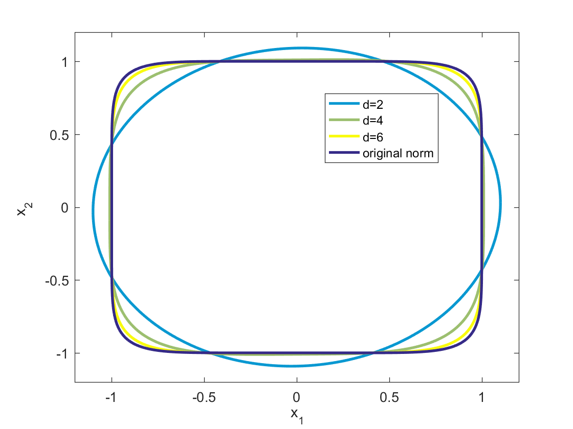
(a) p-norm approximation

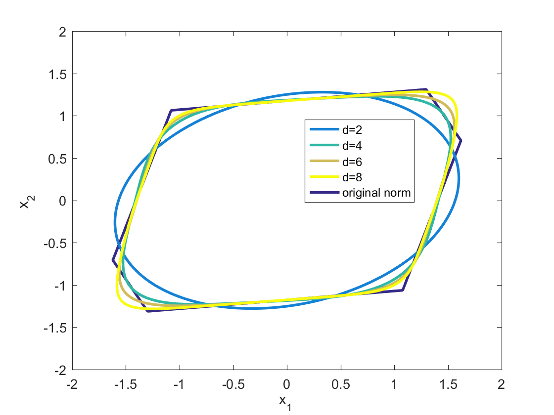
(b) Polytopic norm approximation

Figure 6.2: Approximation of non-polynomial norms by polynomial norms

A similar method could be used for norm regression. In this case, we would have access to data points $x_{1},\ldots,x_{N}$ corresponding to noisy measurements of an underlying unknown norm function. We would then solve the same optimization problem as the one given in (6.17) to obtain a polynomial norm that most closely approximates the noisy data.

6.5.2 Joint spectral radius and stability of linear switched systems

As a second application, we revisit a result from Ahmadi and Jungers from [3, 6] on upperbounding the joint spectral radius of a finite set of matrices. We first review a few notions relating to dynamical systems and linear algebra. The spectral radius $\rho$ of a matrix $A$ is defined as

$$\rho(A)=\lim_{k\rightarrow\infty}||A^{k}||^{1/k}.$$

The spectral radius happens to coincide with the eigenvalue of $A$ of largest magnitude. Consider now the discrete-time linear system $x_{k+1}=Ax_{k}$, where $x_{k}$ is the $n\times 1$ state vector of the system at time $k$. This system is said to be asymptotically stable if for any initial starting state $x_{0}\in\mathbb{R}^{n}$, $x_{k}\rightarrow 0,$ when $k\rightarrow\infty.$ A well-known result connecting the spectral radius of a matrix to the stability of a linear system states that the system $x_{k+1}=Ax_{k}$ is asymptotically stable if and only if $\rho(A)<1$.

In 1960, Rota and Strang introduced a generalization of the spectral radius to a set of matrices. The joint spectral radius (JSR) of a set of matrices $\mathcal{A}\mathrel{\mathop{:}}=\{A_{1},\ldots,A_{m}\}$ is defined as

$$\rho(\mathcal{A})\mathrel{\mathop{:}}=\lim_{k\rightarrow\infty}\max_{\sigma\in\{1,\ldots,m\}^{k}}||A_{\sigma_{k}}\ldots A_{\sigma_{1}}||^{1/k}.$$ (6.18)

Analogously to the case where we have just one matrix, the value of the joint spectral radius can be used to determine stability of a certain type of system, called a switched linear system. A switched linear system models an uncertain and time-varying linear system, i.e., a system described by the dynamics

$$x_{k+1}=A_{k}x_{k},$$

where the matrix $A_{k}$ varies at each iteration within the set $\mathcal{A}$. As done previously, we say that a switched linear system is asymptotically stable if $x_{k}\rightarrow\infty$ when $k\rightarrow\infty$, for any starting state $x_{0}\in\mathbb{R}^{n}$ and any sequence of products of matrices in $\mathcal{A}$. One can establish that the switched linear system $x_{k+1}=A_{k}x_{k}$ is asymtotically stable if and only if $\rho(\mathcal{A})<1$ [101].

Though they may seem similar on many points, a key difference between the spectral radius and the joint spectral radius lies in difficulty of computation: testing whether the spectral radius of a matrix $A$ is less than equal (or strictly less) than $1$ can be done in polynomial time. However, already when $m=2$, the problem of testing whether $\rho(A_{1},A_{2})\leq 1$ is undecidable [31]. An active area of research has consequently been to obtain sufficient conditions for the JSR to be strictly less than one, which, for example, can be checked using semidefinite programming. The theorem that we revisit below is a result of this type. We start first by recalling a Theorem linked to stability of a linear system.

Theorem 6.5.1 (see, e.g., Theorem 8.4 in [91]).

Let $A\in\mathbb{R}^{n\times n}$. Then, $\rho(A)<1$ if and only if there exists a contracting quadratic norm; i.e., a function $V:\mathbb{R}^{n}\rightarrow\mathbb{R}$ of the form $V(x)=\sqrt{x^{T}Qx}$ with $Q\succ 0$, such that $V(Ax)<V(x),\forall x\neq 0.$

The next theorem (from [3, 6]) can be viewed as an extension of Theorem 6.5.1 to the joint spectral radius of a finite set of matrices. It is known that the existence of a contracting quadratic norm is no longer necessary for stability in this case. This theorem show however that the existence of a contracting polynomial norm is.

Theorem 6.5.2 (adapted from [3, 6], Theorem 3.2 ).

Let $\mathcal{A}\mathrel{\mathop{:}}=\{A_{1},\ldots,A_{m}\}$ be a family of $n\times n$ matrices. Then, $\rho(A_{1},\ldots,A_{m})<1$ if and only if there exists a contracting polynomial norm; i.e., a function $V(x)=f^{1/d}(x)$, where $f$ is an n-variate convex and positive definite form of degree $d$, such that $V(A_{i}x)<V(x),~{}\forall x\neq 0$ and $\forall i=1,\ldots,m.$

We remark that in [5], Ahmadi and Jungers show that the degree of $f$ cannot be bounded as a function of $m$ and $n$. This is expected from the undecidability result mentioned before.

Example 6.5.3.

We consider a modification of Example 5.4. in [4] as an illustration of the previous theorem. We would like to show that the joint spectral radius of the two matrices

$$A_{1}=\frac{1}{3.924}\begin{bmatrix}-1&-1\\ 4&0\end{bmatrix},\quad A_{2}=\frac{1}{3.924}\begin{bmatrix}3&3\\ -2&1\end{bmatrix}$$

is strictly less that one.

To do this, we search for a nonzero form $f$ of degree $d$ such that

$$f-(\sum_{i=1}^{n}x_{i}^{2})^{d/2}\text{ sos-convex}$$ (6.19)

$$f(x)-f(A_{i}x)-(\sum_{i=1}^{n}x_{i}^{2})^{d/2}\text{ sos},\text{ for }i=1,2.$$

If problem (6.19) is feasible for some $d$, then $\rho(A_{1},A_{2})<1$. A quick computation using the software package YALMIP [125] and the SDP solver MOSEK [140] reveals that, when $d=2$ or $d=4$, problem (6.19) is infeasible. When $d=6$ however, the problem is feasible and we obtain a polynomial norm $V=f^{1/d}$ whose 1-sublevel set is the outer set plotted in Figure 6.3. We also plot on Figure 6.3 the images of this 1-sublevel set under $A_{1}$ and $A_{2}$. Note that both sets are included in the 1-sublevel set of $V$ as expected. From Theorem 6.5.2, the existence of a polynomial norm implies that $\rho(A_{1},A_{2})<1$ and hence, the pair $\{A_{1},A_{2}\}$ is asymptotically stable.

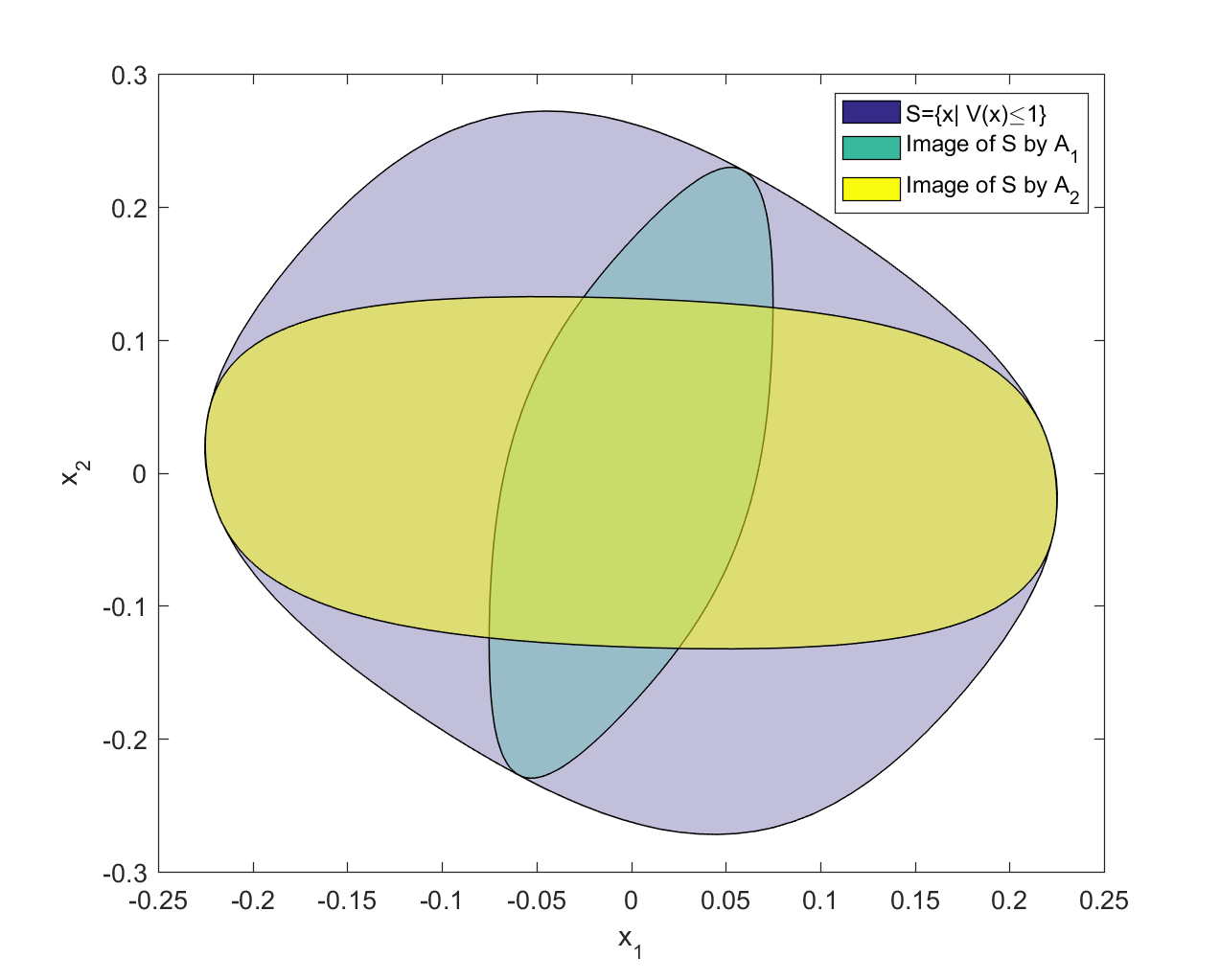
Figure 6.3: Image of the sublevel set of $V$ under $A_{1}$ and $A_{2}$

Remark 6.5.4.

As mentioned previously, problem (6.19) is infeasible for $d=4$. Instead of pushing the degree of $f$ up to 6, one could wonder whether the problem would have been feasible if we had asked that $f$ of degree $d=4$ be $r$-sos-convex for some fixed $r\geq 1$. As mentioned before, in the particular case where $n=2$ (which is the case at hand here), the notions of convexity and sos-convexity coincide; see [12]. As a consequence, one can only hope to make problem (6.19) feasible by increasing the degree of $f$.

6.6 Future directions

In this chapter, we provided semidefinite programming-based conditions under which we could test whether the $d^{th}$ root of a degree-$d$ form is a polynomial norm (Section 6.4.3), and semidefinite programming-based conditions under which we could optimize over the set of forms with positive definite Hessians (Section 6.4.4). A clear gap emerged between forms which are strictly convex and those which have a positive definite Hessian, the latter being a sufficient (but not necessary) condition for the former. This leads us to consider the following two open problems.

Open Problem 6.6.1.

We have given a semidefinite programming hierarchy for optimizing over a subset of polynomial norms. Is there a semidefinite programming hierarchy that optimizes over all polynomial norms?

Open Problem 6.6.2.

Helton and Nie have shown in [89] that sublevel sets of forms that have positive definite Hessians are SDP-representable. This means that we can optimize linear functions over these sets using semidefinite programming. Is the same true for sublevel sets of all polynomial norms?

On the application side, it might be interesting to investigate how one can use polynomial norms to design regularizers in machine learning applications. Indeed, a very popular use of norms in optimization is as regularizers, with the goal of imposing additional structure (e.g., sparsity or low-rankness) on optimal solutions. One could imagine using polynomial norms to design regularizers that are based on the data at hand in place of more generic regularizers such as the 1-norm. Regularizer design is a problem that has already been considered (see, e.g., [21, 39]) but not using polynomial norms. This can be worth exploring as we have shown that polynomial norms can approximate any norm with arbitrary accuracy, while remaining differentiable everywhere (except at the origin), which can be beneficial for optimization purposes.

Chapter 7 Geometry of 3D Environments and Sum of Squares Polynomials

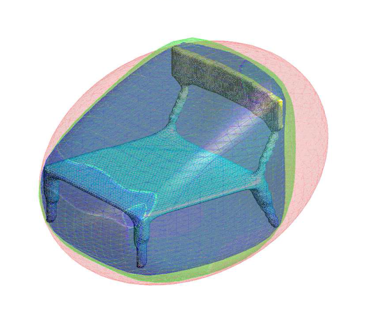
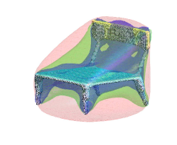
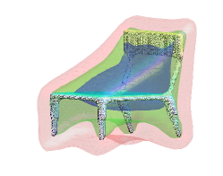
Figure 7.1: Sublevel sets of sos-convex polynomials of increasing degree (left); sublevel sets of sos polynomials of increasing nonconvexity (middle); growth and shrinkage of an sos-body with sublevel sets (right)

7.1 Introduction

A central problem in robotics, computer graphics, virtual and augmented reality (VR/AR), and many applications involving complex physics simulations is the accurate, real-time determination of proximity relationships between three-dimensional objects [64] situated in a cluttered environment. In robot navigation and manipulation tasks, path planners need to compute a dynamically feasible trajectory connecting an initial state to a goal configuration while avoiding obstacles in the environment. In VR/AR applications, a human immersed in a virtual world may wish to touch computer generated objects that must respond to contacts in physically realistic ways. Likewise, when collisions are detected, 3D gaming engines and physics simulators (e.g., for molecular dynamics) need to activate appropriate directional forces on interacting entities. All of these applications require geometric notions of separation and penetration between representations of three-dimensional objects to be continuously monitored.

A rich class of computational geometry problems arises in this context, when 3D objects are outer approximated by convex or nonconvex bounding volumes [75, 134, 108]. In the case where the bounding volumes are convex, the Euclidean distance between them can be computed very precisely, providing a reliable certificate of safety for the objects they enclose. In the case where the bounding volumes are nonconvex, distance computation can be done either approximately via convex decomposition heuristics [120, 133] which cover the volumes by a finite union of convex shapes, or exactly by using more elaborate algebraic optimization hierarchies that we discuss in this chapter. When 3D objects overlap, quantitative measures of degree of penetration are needed in order to optimally resolve collisions, e.g., by a gradient-based trajectory optimizer. Multiple such measures have been proposed in the literature. The penetration depth is the minimum magnitude translation that brings the overlapping objects out of collision. The growth distance [150] is the minimum shrinkage of the two bodies required to reduce volume penetration down to merely surface touching. Efficient computation of penetration measures is also a problem of interest to this chapter.

7.1.1 Contributions and organization of the chapter

In this work, we propose to represent the geometry of a given 3D environment comprising multiple static or dynamic rigid bodies using sublevel sets of polynomials. The chapter is organized as follows: In Section 7.2, we provide an overview of the algebraic concepts of sum of squares (sos) and sum of squares-convex (sos-convex) polynomials as well as their relation to semidefinite programming and polynomial optimization. In Section 7.3, we consider the problem of containing a cloud of 3D points with tight-fitting convex or nearly convex sublevel sets of polynomials. In particular, we propose and justify a new volume minimization heuristic for these sublevel sets which empirically results in tighter fitting polynomials than previous proposals [130], [113]. Additionally, we give a procedure for explicitly tuning the extent of convexity imposed on these sublevel set bounding volumes using sum of squares optimization techniques. If convexity is imposed, we refer to them as sos-convex bodies; if it is not, we term them simply as sos-bodies. (See Section 7.2 for a more formal definition.) We show that the bounding volumes we obtain are highly compact and adapt to the shape of the data in more flexible ways than canned convex primitives typically used in standard bounding volume hierarchies; see Table 7.1. The construction of our bounding volumes involves small-scale semidefinite programs (SDPs) that can fit, in an offline preprocessing phase, 3D meshes with tens of thousands of data points in a few seconds. In Section 7.4, we give sum of squares algorithms for measuring notions of separation or penetration, including Euclidean distance and growth distance [150], of two bounding volumes representing obstacles. We show that even when convexity is lacking, we can efficiently compute (often tight) lower bounds on these measures. In Section 7.5, we consider the problem of grouping several obstacles (i.e., bounding volumes) within one, with the idea of making a map of the 3D environment with a lower level of resolution. A semidefinite programming based algorithm for this purpose is proposed and demonstrated via an example.

7.1.2 Preview of some experiments

Figure 7.1 gives a preview of some of the methods developed in this chapter using as an example a 3D chair point cloud. On the left, we enclose the chair within the 1-sublevel set of three sos-convex polynomials with increasing degree ($2$, $4$ and $6$) leading to correspondingly tighter fits. The middle plot presents the 1-sublevel set of three degree-6 sos polynomials with increasing nonconvexity showing how tighter representations can be obtained by relaxing convexity. The right plot shows the 2, 1, and 0.75 sublevel sets of a single degree-6 sos polynomial; the 1-sublevel set colored green encloses the chair, while greater or lower values of the level set define grown and shrunk versions of the object. The computation of Euclidean distances and sublevel-based measures of separation and penetration can be done in a matter of milliseconds with techniques described in this chapter.

7.2 Sum of squares and sos-convexity

In this section, we briefly review the notions of sum of squares polynomials, sum of squares-convexity, and polynomial optimization which will all be central to the geometric problems we discuss later. We refer the reader to the recent monograph [112] for a more detailed overview of the subject.

Throughout, we will denote the set of $n\times n$ symmetric matrices by $S^{n\times n}$ and the set of degree-$2d$ polynomials with real coefficients by $\mathbb{R}_{2d}[x]$. We say that a polynomial $p(x_{1},\ldots,x_{n})\in\mathbb{R}_{2d}[x]$ is nonnegative if $p(x_{1},\ldots,x_{n})\geq 0,\forall x\in\mathbb{R}^{n}$. In many applications (including polynomial optimization that we will cover later), one would like to constrain certain coefficients of a polynomial so as to make it nonnegative. Unfortunately, even testing whether a given polynomial (of degree $2d\geq 4$) is nonnegative is NP-hard. As a consequence, we would like to replace the intractable condition that $p$ be nonnegative by a sufficient condition for it that is more tractable. One such condition is for the polynomial to have a sum of squares decomposition. We say that a polynomial $p$ is a sum of squares (sos) if there exist polynomials $q_{i}$ such that $p=\sum_{i}q_{i}^{2}$. From this definition, it is clear that any sos polynomial is nonnegative, though not all nonnegative polynomials are sos; see, e.g., [165],[115] for some counterexamples. Furthermore, requiring that a polynomial $p$ be sos is a computationally tractable condition as a consequence of the following characterization: A polynomial $p$ of degree $2d$ is sos if and only if there exists a positive semidefinite matrix $Q$ such that $p(x)=z(x)^{T}Qz(x),$ where $z(x)$ is the vector of all monomials of degree up to $d$ [152]. The matrix $Q$ is sometimes called the Gram matrix of the sos decomposition and is of size $\binom{n+d}{d}\times\binom{n+d}{d}$. (Throughout the chapter, we let $N\mathcal{\mathop{:}}=\binom{n+d}{d}.$) The task of finding a positive semidefinite matrix $Q$ that makes the coefficients of $p$ all equal to the coefficients of $z(x)^{T}Qz(x)$ is a semidefinite programming problem, which can be solved in polynomial time to arbitrary accuracy [192].

The concept of sum of squares can also be used to define a sufficient condition for convexity of polynomials known as sos-convexity. We say that a polynomial $p$ is sos-convex if the polynomial $y^{T}\nabla^{2}p(x)y$ in $2n$ variables $x$ and $y$ is a sum of squares. Here, $\nabla^{2}p(x)$ denotes the Hessian of $p$, which is a symmetric matrix with polynomial entries. For a polynomial of degree $2d$ in $n$ variables, one can check that the dimension of the Gram matrix associated to the sos-convexity condition is $\tilde{N}\mathcal{\mathop{:}}=n\cdot\binom{n+d-1}{d-1}$. It follows from the second order characterization of convexity that any sos-convex polynomial is convex, as $y^{T}\nabla^{2}p(x)y$ being sos implies that $\nabla^{2}p(x)\succeq 0,~{}\forall x.$ The converse however is not true, though convex but not sos-convex polynomials are hard to find in practice; see [12]. Through its link to sum of squares, it is easy to see that testing whether a given polynomial is sos-convex is a semidefinite program. By contrast, testing whether a polynomial of degree $2d\geq 4$ is convex is NP-hard [10].

A polynomial optimization problem is a problem of the form

$$\min_{x\in K}p(x),$$ (7.1)

where the objective $p$ is a (multivariate) polynomial and the feasible set $K$ is a basic semialgebraic set; i.e., a set defined by polynomial inequalities:

$$K:=\{x~{}|~{}g_{i}(x)\geq 0,i=1,\ldots,m\}.$$

It is straightforward to see that problem (7.1) can be equivalently formulated as that of finding the largest constant $\gamma$ such that $p(x)-\gamma\geq 0,\forall x\in K.$ It is known that, under mild conditions (specifically, under the assumption that $K$ is Archimedean [115]), the condition $p(x)-\gamma>0,\forall x\in K$, is equivalent to the existence of sos polynomials $\sigma_{i}(x)$ such that $p(x)-\gamma=\sigma_{0}(x)+\sum_{i=1}^{m}\sigma_{i}(x)g_{i}(x)$. Indeed, it is at least clear that if $x\in K$, i.e., $g_{i}(x)\geq 0$, then $\sigma_{0}(x)+\sum_{i=1}^{m}\sigma_{i}(x)g_{i}(x)\geq 0$ which means that $p(x)-\gamma\geq 0$. The converse is less trivial and is a consequence of the Putinar Positivstellensatz [162]. Using this result, problem (7.1) can be rewritten as

$$\underset{\gamma,\sigma_{i}}{\max}~{}\gamma$$

$$\text{s.t. }p(x)-\gamma=\sigma_{0}+\sum_{i=1}^{m}\sigma_{i}(x)g_{i}(x),$$ (7.2)

$$\sigma_{i}\text{ sos, }i=0,\ldots,m.$$

For any fixed upper bound on the degrees of the polynomials $\sigma_{i}$, this is a semidefinite programming problem which produces a lower bound on the optimal value of (7.1). As the degrees of $\sigma_{i}$ increase, these lower bounds are guaranteed to converge to the true optimal value of (7.1). Note that we are making no convexity assumptions about the polynomial optimization problem and yet solving it globally through a sequence of semidefinite programs.

Sum of squares and polynomial optimization in robotics. We remark that sum of squares techniques have recently found increasing applications to a whole host of problems in robotics, including constructing Lyapunov functions [13], locomotion planning [106], design and verification of provably safe controllers [131, 132], grasping and manipulation [50, 159, 202], robot-world calibration [88], and inverse optimal control [156], among others.

We also remark that a different use of sum of squares optimization for finding minimum bounding volumes that contain semialgebraic sets has been considered in [49, 48] along with some interesting control applications (see Section 7.5 for a brief description).

7.3 3D point cloud containment

Throughout this section, we are interested in finding a body of minimum volume, parametrized as the 1-sublevel set of a polynomial of degree $2d$, which encloses a set of given points $\{x_{1},\ldots,x_{m}\}$ in $\mathbb{R}^{n}$.

7.3.1 Convex sublevel sets

We focus first on finding a convex bounding volume. Convexity is a common constraint in the bounding volume literature and it makes certain tasks (e.g., distance computation among the different bodies) simpler. In order to make a set of the form $\{x\in\mathbb{R}^{3}|\ p(x)\leq 1\}$ convex, we will require the polynomial $p$ to be convex. (Note that this is a sufficient but not necessary condition.) Furthermore, to have a tractable formulation, we will replace the convexity condition with an sos-convexity condition as described previously. Even after these relaxations, the problem of minimizing the volume of our sublevel sets remains a difficult one. The remainder of this section discusses several heuristics for this task.

The Hessian-based approach

In [130], Magnani et al. propose the following heuristic to minimize the volume of the 1-sublevel set of an sos-convex polynomial:

$$\min_{p\in\mathbb{R}_{2d}[x],H\in S^{\tilde{N}\times\tilde{N}}}-\log\det(H)$$ (7.3)

s.t. $$p\text{ sos},$$

$$y^{T}\nabla^{2}p(x)y=w(x,y)^{T}Hw(x,y),~{}H\succeq 0,$$

$$p(x_{i})\leq 1,i=1,\ldots,m,$$

where $w(x,y)$ is a vector of monomials in $x$ and $y$ of degree $1$ in $y$ and $d-1$ in $x$. This problem outputs a polynomial $p$ whose 1-sublevel set corresponds to the bounding volume that we are interested in. A few remarks on this formulation are in order:

• The last constraint simply ensures that all the data points are within the 1-sublevel set of $p$ as required.

• The second constraint imposes that $p$ be sos-convex. The matrix $H$ is the Gram matrix associated with the sos condition on $y^{T}\nabla^{2}p(x)y$.

• The first constraint requires that the polynomial $p$ be sos. This is a necessary condition for boundedness of (7.3) when $p$ is parametrized with affine terms. To see this, note that for any given positive semidefinite matrix $Q$, one can always pick the coefficients of the affine terms in such a way that the constraint $p(x_{i})\leq 1$ for $i=1,\ldots,m$ be trivially satisfied. Likewise one can pick the remaining coefficients of $p$ in such a way that the sos-convexity condition is satisfied. The restriction to sos polynomials, however, can be done without loss of generality. Indeed, suppose that the minimum volume sublevel set was given by $\{x~{}|~{}p(x)\leq 1\}$ where $p$ is an sos-convex polynomial. As $p$ is convex and nonaffine, $\exists\gamma\geq 0$ such that $p(x)+\gamma\geq 0$ for all $x$. Define now $q(x)\mathrel{\mathop{:}}=\frac{p(x)+\gamma}{1+\gamma}.$ We have that $\{x~{}|~{}p(x)\leq 1\}=\{x~{}|~{}q(x)\leq 1\}$, but here, $q$ is sos as it is sos-convex and nonnegative [89, Lemma 8].

The objective function of the above formulation is motivated in part by the degree $2d=2$ case. Indeed, when $2d=2$, the sublevel sets of convex polynomials are ellipsoids of the form $\{x~{}|~{}x^{T}Px+b^{T}x+c\leq 1\}$ and their volume is given by $\frac{4}{3}\pi\cdot\sqrt{\det(P^{-1})}$. Hence, by minimizing $-\log\det(P)$, we would exactly minimize volume. As the matrix $P$ above is none other than the Hessian of the quadratic polynomial $x^{T}Px+b^{T}x+c$ (up to a multiplicative constant), this partly justifies the formulation given in [130]. Another justification for this formulation is given in [130] itself and relates to curvature of the polynomial $p$. Indeed, the curvature of $p$ at a point $x$ along a direction $y$ is proportional to $y^{T}\nabla^{2}p(x)y$. By imposing that $y^{T}\nabla^{2}p(x)y=w(x,y)^{T}Hw(x,y),$ with $H\succeq 0$, and then maximizing $\log(\det(H))$, this formulation seeks to increase the curvature of $p$ along all directions so that its 1-sublevel set can get closer to the points $x_{i}$. Note that curvature maximization in all directions without regards to data distribution can be counterproductive in terms of tightness of fit, particularly in regions where the data geometry is flat (an example of this is given in Figure 7.3).

A related minimum volume heuristic that we will also experiment with replaces the $\log\det$ objective with a linear one. More specifically, we introduce an extra decision variable $V\in S^{\tilde{N}\times\tilde{N}}$ and minimize $\mbox{trace}(V)$ while adding an additional constraint $\begin{bmatrix}V&I\\ I&H\end{bmatrix}\succeq 0.$ Using the Schur complement, the latter constraint can be rewritten as $V\succeq H^{-1}$. As a consequence, this trace formulation minimizes the sum of the inverse of the eigenvalues of $H$ whereas the $\log\det$ formulation described in (7.3) minimizes the product of the inverse of the eigenvalues.

Our approach

We propose here an alternative heuristic for obtaining a tight-fitting convex body containing points in $\mathbb{R}^{n}.$ Empirically, we validate that it tends to consistently return convex bodies of smaller volume than the ones obtained with the methods described above (see Figure 7.3 below for an example). It also generates a relatively smaller convex optimization problem. Our formulation is as follows:

$$\min_{p\in\mathbb{R}_{2d}[x],P\in S^{N\times N}}-\log\det(P)$$

s.t.

$$p(x)=z(x)^{T}Pz(x),P\succeq 0,$$

$$p\text{ sos-convex},$$ (7.4)

$$p(x_{i})\leq 1,i=1,\ldots,m.$$

One can also obtain a trace formulation of this problem by replacing the $\log\det$ objective by a trace one as it was done in the previous paragraph.

Note that the main difference between (7.3) and (7.4) lies in the Gram matrix chosen for the objective function. In (7.3), the Gram matrix comes from the sos-convexity constraint, whereas in (7.4), the Gram matrix is generated by the sos constraint.

In the case where the polynomial is quadratic and convex, we saw that the formulation (7.3) is exact as it finds the minimum volume ellipsoid containing the points. It so happens that the formulation given in (7.4) is also exact in the quadratic case, and, in fact, both formulations return the same optimal ellipsoid. As a consequence, the formulation given in (7.4) can also be viewed as a natural extension of the quadratic case.

To provide more intuition as to why this formulation performs well, we interpret the 1-sublevel set

$$S\mathrel{\mathop{:}}=\{x~{}|~{}p(x)\leq 1\}$$

of $p$ as the preimage of some set whose volume is being minimized. More precisely, consider the set

$$T_{1}=\{z(x)\in\mathbb{R}^{N}~{}|~{}x\in\mathbb{R}^{n}\}$$

which corresponds to the image of $\mathbb{R}^{n}$ under the monomial map $z(x)$ and the set

$$T_{2}=\{y\in\mathbb{R}^{N}~{}|~{}y^{T}Py\leq 1\},$$

for a positive semidefinite matrix $P$ such that $p(x)=z(x)^{T}Pz(x).$ Then, the set $S$ is simply the preimage of the intersection of $T_{1}$ and $T_{2}$ through the mapping $z$. Indeed, for any $x\in S$, we have $p(x)=z(x)^{T}Pz(x)\leq 1$. The hope is then that by minimizing the volume of $T_{2}$, we will minimize volume of the intersection $T_{1}\cap T_{2}$ and hence that of its preimage through $z$, i.e., the set $S.$

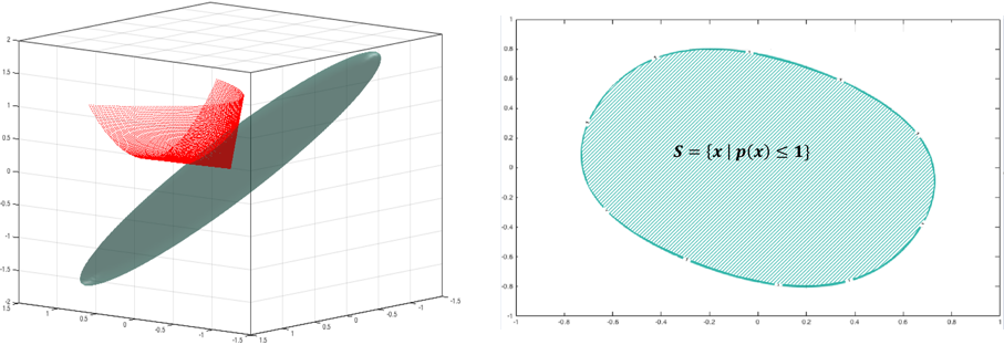
Figure 7.2: An illustration of the intuition behind the approach in Section 7.3.1: the sets $T_{1}$ and $T_{2}$ (left) and $S$ (right)

We illustrate this idea in Figure 7.2. Here, we have generated a random $3\times 3$ positive semidefinite matrix $P$ and a corresponding bivariate degree-4 sos polynomial $p(x_{1},x_{2})=z(x_{1},x_{2})^{T}Pz(x_{1},x_{2})$, where $z(x_{1},x_{2})=(x_{1}^{2},x_{1}x_{2},x_{2}^{2})^{T}$ is a map from $\mathbb{R}^{2}$ to $\mathbb{R}^{3}$. We have drawn in red the image of $\mathbb{R}^{2}$ under $z$ and in green the ellipsoid $\{y\in\mathbb{R}^{3}~{}|~{}y^{T}Py\leq 1\}.$ The preimage of the intersection of both sets seen in Figure 7.2 on the right corresponds to the 1-sublevel set of $p.$

7.3.2 Relaxing convexity

Though containing a set of points with a convex sublevel set has its advantages, it is sometimes necessary to have a tighter fit than the one provided by a convex body, particularly if the object of interest is highly nonconvex. One way of handling such scenarios is via convex decomposition methods [120, 133], which would enable us to represent the object as a union of sos-convex bodies. Alternatively, one can aim for problem formulations where convexity of the sublevel sets is not imposed. In the remainder of this subsection, we first review a recent approach from the literature to do this and then present our own approach which allows for controlling the level of nonconvexity of the sublevel set.

The inverse moment approach

In very recent work [113], Lasserre and Pauwels propose an approach for containing a cloud of points with sublevel sets of polynomials (with no convexity constraint). Given a set of data points $x_{1},\ldots,x_{m}\in\mathbb{R}^{n}$, it is observed in that paper that the sublevel sets of the degree $2d$ sos polynomial

$$p_{\mu,d}(x)\mathrel{\mathop{:}}=z(x)^{T}M_{d}(\mu(x_{1},\ldots,x_{m}))^{-1}z(x),$$ (7.5)

tend to take the shape of the data accurately. Here, $z(x)$ is the vector of all monomials of degree up to $d$ and $M_{d}(\mu(x_{1},\ldots,x_{m}))$ is the moment matrix of degree $d$ associated with the empirical measure $\mu\mathrel{\mathop{:}}=\frac{1}{m}\sum_{i=1}^{m}\delta_{x_{i}}$ defined over the data. This is an $\binom{n+d}{d}\times\binom{n+d}{d}$ symmetric positive semidefinite matrix which can be cheaply constructed from the data $x_{1},\ldots,x_{m}\in\mathbb{R}^{n}$ (see [113] for details). One very nice feature of this method is that to construct the polynomial $p_{\mu,d}$ in (7.5) one only needs to invert a matrix (as opposed to solving a semidefinite program as our approach would require) after a single pass over the point cloud. The approach however does not a priori provide a particular sublevel set of $p_{\mu,d}$ that is guaranteed to contain all data points. Hence, once $p_{\mu,d}$ is constructed, one could slowly increase the value of a scalar $\gamma$ and check whether the $\gamma$-sublevel set of $p_{\mu,d}$ contains all points.

Our approach and controlling convexity

An advantage of our proposed formulation (7.4) is that one can easily drop the sos-convexity assumption in the constraints and thereby obtain a sublevel set which is not necessarily convex. This is not an option for formulation (7.3) as the Gram matrix associated to the sos-convexity constraint intervenes in the objective.

Note that in neither this formulation nor the inverse moment approach of Lasserre and Pauwels, does the optimizer have control over the shape of the sublevel sets produced, which may be convex or far from convex. For some applications, it is useful to control in some way the degree of convexity of the sublevel sets obtained by introducing a parameter which when increased or decreased would make the sets more or less convex. This is what our following proposed optimization problem does via the parameter $c$, which corresponds in some sense to a measure of convexity:

$$\min_{p\in\mathbb{R}_{2d}[x],P\in S^{N\times N}}-\log\det(P)$$

s.t.

$$p=z(x)^{T}Pz(x),P\succeq 0$$ (7.6)

$$p(x)+c(\sum_{i}x_{i}^{2})^{d}\text{ sos-convex}.$$

$$p(x_{i})\leq 1,i=1,\ldots,m.$$

Note that when $c=0$, the problem we are solving corresponds exactly to (7.4) and the sublevel set obtained is convex. When $c>0$, we allow for nonconvexity of the sublevel sets. Note that this is a consequence of $(\sum_{i}x_{i}^{2})^{d}$ being a strictly convex function, which can offset the nonconvexity of $p$. As we decrease $c$ towards zero, we obtain sublevel sets which get progressively more and more convex.

7.3.3 Bounding volume numerical experiments

Figure 7.1 (left) shows the 1-sublevel sets of sos-convex bodies with degrees $2$, $4$, and $6$. A degree-$6$ polynomial gives a much tighter fit than an ellipsoid (degree 2). In the middle figure, we freeze the degree to be $6$ and increase the convexity parameter $c$ in the relaxed convexity formulation of problem (7.6); the 1-sublevel sets of the resulting sos polynomials with $c=0,10,100$ are shown. It can be seen that the sublevel sets gradually bend to better adapt to the shape of the object. The right figure shows the $2,1,$ and $0.75$ sublevel sets of a degree-$6$ polynomial obtained by fixing $c=10$ in problem (7.6): the shape is retained as the body is expanded or contracted.

Figure 7.3 shows 1-sublevel sets of two degree-6 sos-convex polynomials. In red, we have plotted the sublevel set corresponding to maximizing curvature as explained in Section 7.3.1. In green, we have plotted the sublevel set generated by our approach as explained in Section 7.3.1. Note that our method gives a tighter-fitting sublevel set, which is in part a consequence of the flat data geometry for which the maximum curvature heuristic does not work as well.

Figure 7.3: Comparison of degree-6 bounding volumes: our approach as described in Section 7.3.1 (green sublevel set) produces a tighter fitting bounding volume than the approach given in [130] and reviewed in Section 7.3.1 (red sublevel set).

In Table 7.1, we provide a comparison of various bounding volumes on Princeton Shape Benchmark datasets [180]. It can be seen that sos-convex bodies generated by higher degree polynomials provide much tighter fits than spheres or axis-aligned bounding boxes (AABB) in general. The proposed minimum volume heuristic of our formulation in (7.4) works better than that proposed in [130] (see (7.3)). In both formulations, typically, the log-determinant objective outperforms the trace objective. The convex hull is the tightest possible convex body. However, for smooth objects like the vase, the number of vertices describing the convex hull can be a substantial fraction of the original number of points in the point cloud. When convexity is relaxed, a degree-6 sos polynomial compactly described by just $84$ coefficients gives a tighter fit than the convex hull. For the same degree, solutions to our formulation (7.6) with a positive value of $c$ outperform the inverse moment construction of [113].

The bounding volume construction times are shown in Figure 7.4 for sos-convex chair models. In comparison to the volume heuristics of [130], our heuristic runs noticeably faster as soon as degree exceeds $6$. We believe that this may come from the fact that the decision variable featuring in the objective in our case is a matrix of size $N\times N$, where $N=\binom{n+d}{d}$, whereas the decision variable featuring in the objective of [130] is of size $\tilde{N}\times\tilde{N},$ where $\tilde{N}=n\cdot\binom{n+d-1}{d-1}>N.$ Our implementation uses YALMIP [125] with the splitting conic solver (SCS) [149] as its backend SDP solver (run for 2500 iterations). Note that the inverse moment approach of [113] is the fastest as it does not involve any optimization and makes just one pass over the point cloud. However, this approach is not guaranteed to return a convex body, and for nonconvex bodies, tighter fitting polynomials can be estimated using log-determinant or trace objectives on our problem (7.6).

	Object (id in [180])		Human (10)	Chair (101)	Hand (181)	Vase (361)	Octopus (121)
	$\#$ points/vertices in cvx hull		9508/364	8499/320	7242/ 652	14859/1443	5944/414
Section	Bounding Body $\downarrow$	Objective fcn $\downarrow$	Volume $\downarrow$
	Convex-Hull		0.29	0.66	0.36	0.91	0.5
	Sphere		3.74	3.73	3.84	3.91	4.1
	AABB		0.59	1.0	0.81	1.73	1.28
	sos-convex ($2d=2$)	$logdet$	0.58	1.79	0.82	1.16	1.30
		$trace$	0.97	1.80	1.40	1.2	1.76
	sos-convex ($2d=4$)	$logdet(\mathbf{H}^{-1})$	0.57	1.55	0.69	1.13	1.04
		$trace(\mathbf{H}^{-1})$	0.56	2.16	1.28	1.09	3.13
		$logdet(\mathbf{P}^{-1})$	0.44	1.19	0.53	1.05	0.86
7.3.1		$trace(\mathbf{P}^{-1})$	0.57	1.25	0.92	1.09	1.02
	sos-convex ($2d=6$)	$logdet(\mathbf{H}^{-1})$	0.57	1.27	0.58	1.09	0.93
		$trace(\mathbf{H}^{-1})$	0.56	1.30	0.57	1.09	0.87
		$logdet(\mathbf{P}^{-1})$	0.41	1.02	0.45	0.99	0.74
		$trace(\mathbf{P}^{-1})$	0.45	1.21	0.48	1.03	0.79
	Inverse-Moment ($2d=2$)		4.02	1.42	2.14	1.36	1.74
	Inverse-Moment ($2d=4$)		1.53	0.95	0.90	1.25	0.75
7.3.2	Inverse-Moment ($2d=6$)		0.48	0.54	0.58	1.10	0.57
	sos ($2d=4,c=10$)	$logdet(\mathbf{P}^{-1})$	0.38	0.72	0.42	1.05	0.63
		$trace(\mathbf{P}^{-1})$	0.51	0.78	0.48	1.11	0.71
	sos ($2d=6,c=10$)	$logdet(\mathbf{P}^{-1})$	0.35	0.49	0.34	0.92	0.41
		$trace(\mathbf{P}^{-1})$	0.37	0.56	0.39	0.99	0.54
	sos ($2d=4,c=100$)	$logdet(\mathbf{P}^{-1})$	0.36	0.64	0.39	1.05	0.46
7.3.2		$trace(\mathbf{P}^{-1})$	0.42	0.74	0.46	1.10	0.54
	sos ($2d=6,c=100$)	$logdet(\mathbf{P}^{-1})$	0.21	0.21	0.26	0.82	0.28
		$trace(\mathbf{P}^{-1})$	0.22	0.30	0.29	0.85	0.37

Table 7.1: Comparison of the volume of various bounding bodies obtained from different techniques

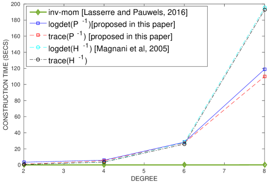
Figure 7.4: Bounding volume construction times

7.4 Measures of separation and penetration

7.4.1 Euclidean distance

In this section, we are interested in computing the Euclidean distance between two basic semialgebraic sets

$$\mathcal{S}_{1}\mathcal{\mathop{:}}=\{x\in\mathbb{R}^{n}~{}|~{}g_{1}(x)\leq 1,\ldots,g_{m}\leq 1\},$$

and

$$\mathcal{S}_{2}\mathcal{\mathop{:}}=\{x\in\mathbb{R}^{n}~{}|~{}h_{1}(x)\leq 1,\ldots,h_{r}\leq 1\}$$

(where $g_{1},\ldots,g_{m}$ and $h_{1},\ldots,h_{r}$ are polynomials). This can be written as the following polynomial optimization problem:

$$\min_{x\in\mathcal{S}_{1},y\in\mathcal{S}_{2}}||x-y||_{2}^{2}.$$ (7.7)

We will tackle this problem by applying the sos hierarchy described at the end of Section 7.2. This will take the form of the following hierarchy of semidefinite programs

$$\max_{\gamma\in\mathbb{R},\tau_{i},\xi_{j}}\gamma$$ (7.8)

$$||x-y||_{2}^{2}-\gamma-\sum_{i=1}^{m}\tau_{i}(x,y)(1-g_{i}(x))$$

$$\hskip 56.9055pt-\sum_{j=1}^{r}\xi_{j}(x,y)(1-h_{j}(y))\text{ sos},$$

$$\tau_{i}(x,y),~{}\xi_{j}(x,y)\text{ sos },\forall i,\forall j,$$

where in the $d$-th level of the hierarchy, the degree of all polynomials $\tau_{i}$ and $\xi_{j}$ is upper bounded by $d$. Observe that the optimal value of each SDP produces a lower bound on (7.7) and that when $d$ increases, this lower bound can only improve.

Amazingly, in all examples we tried (independently of convexity of $\mathcal{S}_{1}$ and $\mathcal{S}_{2}$), the 0-th level of the hierarchy was already exact (though we were unable to prove this). By this we mean that the optimal value of (7.8) exactly matched that of (7.7), already when the degree of the polynomials $\tau_{i}$ and $\xi_{j}$ was zero; i.e., when $\tau_{i}$ and $\xi_{j}$ were nonnegative scalars. An example of this phenomenon is given in Figure 7.5 where the green bodies are each a (highly nonconvex) sublevel set of a quartic polynomial.

When our SDP relaxation is exact, we can recover the points $x^{*}$ and $y^{*}$ where the minimum distance between sets is achieved from the eigenvector corresponding to the zero eigenvalue of the Gram matrix associated with the first sos constraint in (7.8). This is what is done in Figure 7.5.

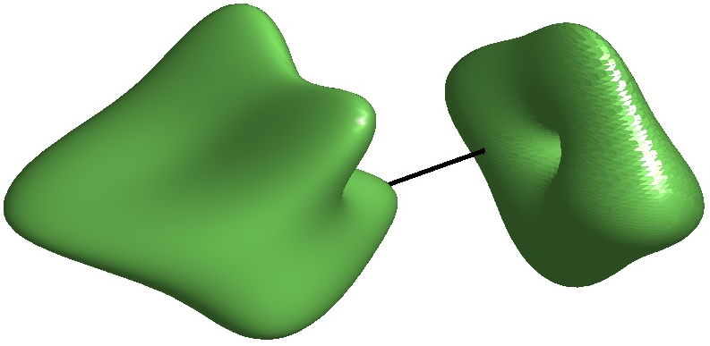
Figure 7.5: Minimum distance between two (nonconvex) sublevel sets of degree-4 polynomials

The sos-convex case. One important special case where we know that the 0-th level of the sos hierarchy in (7.8) is guaranteed to be exact is when the defining polynomials $g_{i}$ and $h_{i}$ of $\mathcal{S}_{1}$ and $\mathcal{S}_{2}$ are sos-convex. This is a corollary of the fact that the 0-th level sos relaxation is known to be tight for the general polynomial optimization problem in (7.1) if the polynomials $p$ and $-g_{i}$ involved in the description of $K$ there are sos-convex; see [110]. An example of the computation of the minimum distance between two degree-6 sos-convex bodies enclosing human and chair 3D point clouds is given below, together with the points achieving the minimum distance.

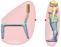
Figure 7.6: Minimum distance between two convex sublevel sets of degree-6 polynomials

Using MATLAB’s fmincon active-set solver, the time required to compute the distance between two sos-convex bodies ranges from around 80 milliseconds to 340 milliseconds seconds as the degree is increased from $2$ to $8$; see Table 7.2. We believe that the execution time can be improved by an order of magnitude with more efficient polynomial representations, warm starts for repeated queries, and reduced convergence tolerance for lower-precision results.

degree	2	4	6	8
time (secs)	0.08	0.083	0.13	0.34

Table 7.2: Euclidean distance query times for sos-convex sets.

7.4.2 Penetration measures for overlapping bodies

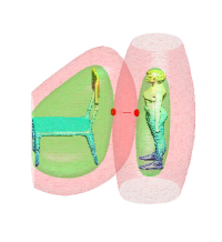
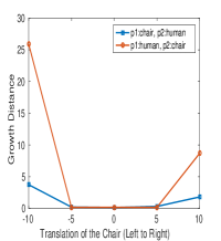
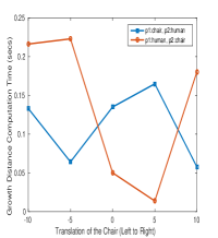
Figure 7.7: Growth distances for separated (left) or overlapping (second-left) sos-convex bodies; growth distance as a function of the position of the chair (second-right); time taken to solve (7.9) with warm-start (right)

As another application of sos-convex polynomial optimization problems, we discuss a problem relevant to collision avoidance. Here, we assume that our two bodies $\mathcal{S}_{1}$, $\mathcal{S}_{2}$ are of the form $\mathcal{S}_{1}\mathrel{\mathop{:}}=\{x~{}|~{}p_{1}(x)\leq 1\}$ and $\mathcal{S}_{2}\mathrel{\mathop{:}}=\{x~{}|~{}p_{2}(x)\leq 1\},$ where $p_{1},p_{2}$ are sos-convex. As shown in Figure 7.1 (right), by varying the sublevel value, we can grow or shrink the sos representation of an object. The following convex optimization problem, with optimal value denoted by $d(p_{1}||p_{2})$, provides a measure of separation or penetration between the two bodies:

$$d(p_{1}||p_{2})=\min p_{1}(x)$$

$$\text{s.t. }p_{2}(x)\leq 1.$$ (7.9)

Note that the measure is asymmetric, i.e., $d(p_{1}||p_{2})\neq d(p_{2}||p_{1})$. It is clear that

$$p_{2}(x)\leq 1\Rightarrow p_{1}(x)\geq d(p_{1}||p_{2}).$$

In other words, the sets $\{x~{}|~{}p_{2}(x)\leq 1\}$ and $\{x~{}|~{}p_{1}(x)\leq d(p_{1}||p_{2})\}$ do not overlap. As a consequence, the optimal value of (7.9) gives us a measure of how much we need to shrink the level set defined by $p_{1}$ to eventually move out of contact of the set $\mathcal{S}_{2}$ assuming that the “seed point”, i.e., the minimum of $p_{1}$, is outside ${\cal S}_{2}$. It is clear that,

• if $d(p_{1}||p_{2})>1$, the bounding volumes are separated.

• if $d(p_{1}||p_{2})=1$, the bounding volumes touch.

• if $d(p_{1}||p_{2})<1$, the bounding volumes overlap.

These measures are closely related to the notion of growth models and growth distances [150]. Note that similarly to what is described for the sos-convex case in Section 7.4.1, the optimal solution $d(p_{1}||p_{2})$ to (7.9) can be computed exactly using semidefinite programming, or using a generic convex optimizer. The two leftmost subfigures of Figure 7.7 show a chair and a human bounded by 1-sublevel sets of degree 6 sos-convex polynomials (in green). In both cases, we compute $d(p_{1}||p_{2})$ and $d(p_{2}||p_{1})$ and plot the corresponding minimizers. In the first subfigure, the level set of the chair needs to grow in order to touch the human and vice-versa, certifying separation. In the second subfigure, we translate the chair across the volume occupied by the human so that they overlap. In this case, the level sets need to contract. In the third subfigure, we plot the optimal value of the problem in (7.9) as the chair is translated from left to right, showing how the growth distances dip upon penetration and rise upon separation. The final subfigure shows the time taken to solve (7.9) when warm started from the previous solution. The time taken is of the order of 150 milliseconds without warm starts to 10 milliseconds with warm starts.

7.5 Containment of polynomial sublevel sets

In this section, we show how the sum of squares machinery can be used in a straightforward manner to contain polynomial sublevel sets (as opposed to point clouds) with a convex polynomial level set. More specifically, we are interested in the following problem: Given a basic semialgebraic set

$$\mathcal{S}\mathrel{\mathop{:}}=\{x\in\mathbb{R}^{n}|\ g_{1}(x)\leq 1,\ldots,g_{m}(x)\leq 1\},$$ (7.10)

find a convex polynomial $p$ of degree $2d$ such that

$$\mathcal{S}\subseteq\{x\in\mathbb{R}^{n}|\ p(x)\leq 1\}.$$ (7.11)

Moreover, we typically want the unit sublevel set of $p$ to have small volume. Note that if we could address this question, then we could also handle a scenario where the unit sublevel set of $p$ is required to contain the union of several basic semialgebraic sets (simply by containing each set separately). For the 3D geometric problems under our consideration, we have two applications of this task in mind:

• Convexification: In some scenarios, one may have a nonconvex outer approximation of an obstacle (e.g., obtained by the computationally inexpensive inverse moment approach of Lasserre and Pauwels as described in Section 7.3.2) and be interested in containing it with a convex set. This would e.g. make the problem of computing distances among obstacles more tractable; cf. Section 7.4.

• Grouping multiple obstacles: For various navigational tasks involving autonomous agents, one may want to have a mapping of the obstacles in the environment in varying levels of resolution. A relevant problem here is therefore to group obstacles: this would lead to the problem of containing several polynomial sublevel sets with one.

In order to solve the problem laid out above, we propose the following sos program:

$$\min_{p\in\mathbb{R}_{2d}[x],\tau_{i}\in\mathbb{R}_{2\hat{d}}[x],P\in S^{N\times N}}-\log\det(P)$$

s.t. $$p(x)=z(x)^{T}Pz(x),P\succeq 0,$$

$$p(x)\quad\text{sos-convex,}$$ (7.12)

$$1-p(x)-\sum_{i=1}^{m}\tau_{i}(x)(1-g_{i}(x))\quad\text{sos,}$$ (7.13)

$$\tau_{i}(x)\quad\text{sos,}\quad i=1,\ldots,m.$$ (7.14)

It is straightforward to see that constraints (7.13) and (7.14) imply the required set containment criterion in (7.11). As usual, the constraint in (7.12) ensures convexity of the unit sublevel set of $p$. The objective function attempts to minimize the volume of this set. A natural choice for the degree $2\hat{d}$ of the polynomials $\tau_{i}$ is $2\hat{d}=2d-\min_{i}deg(g_{i})$, though better results can be obtained by increasing this parameter.

An analoguous problem is discussed in recent work by Dabbene, Henrion, and Lagoa [48, 49]. In the paper, the authors want to find a polynomial $p$ of degree $d$ whose 1-superlevel set $\{x~{}|~{}p(x)\geq 1\}$ contains a semialgebraic set $\mathcal{S}$ and has minimum volume. Assuming that one is given a set $B$ containing $\mathcal{S}$ and over which the integrals of polynomials can be efficiently computed, their method involves searching for a polynomial $p$ of degree $d$ which minimizes $\int_{B}p(x)dx$ while respecting the constraints $p(x)\geq 1$ on $\mathcal{S}$ and $p(x)\geq 0$ on $B$. Note that the objective is linear in the coefficients of $p$ and that these last two nonnegativity conditions can be made computationally tractable by using the sum of squares relaxation. The advantage of such a formulation lies in the fact that when the degree of the polynomial $p$ increases, the objective value of the problem converges to the true volume of the set $\mathcal{S}$.

Example. In Figure 7.8, we have drawn in black three random ellipsoids and a degree-4 convex polynomial sublevel set (in yellow) containing the ellipsoids. This degree-4 polynomial was the output of the optimization problem described above where the sos multipliers $\tau_{i}(x)$ were chosen to have degree $2$.

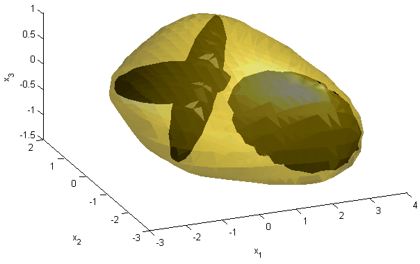
Figure 7.8: Containment of 3 ellipsoids using a sublevel set of a convex degree-4 polynomial

We end by noting that the formulation proposed here is backed up theoretically by the following converse result.

Theorem 7.5.1.

Suppose the set $\mathcal{S}$ in (7.10) is Archimedean and that $\mathcal{S}\subset\{x\in\mathbb{R}^{n}|\ p(x)\leq 1\}.$ Then there exists an integer $\hat{d}$ and sum of squares polynomials $\tau_{1},\ldots,\tau_{m}$ of degree at most $\hat{d}$ such that

$$1-p(x)-\sum_{i=1}^{m}\tau_{i}(x)(1-g_{i}(x))$$ (7.15)

is a sum of squares.

Proof.

The proof follows from a standard application of Putinar’s Positivstellensatz [162] and is omitted. ∎

Chapter 8 Nonnegative polynomials and shape-constrained regression

Unlike the other chapters in this thesis, the paper on which this chapter is based is still in preparation. We recommend that future readers read the submitted version of this chapter if it is available at the time of reading.

8.1 Introduction

Regression is a key problem in statistics and machine learning. Its goal is to estimate relationships between an explained variable (e.g., the price of a second-hand car) and a vector of explanatory variables (e.g., the make, brand, mileage, power, or age of this car). In many applications, one can observe a monotonous dependency between the explained variable and the explanatory variables. Examples arise in many different areas, including medicine, e.g., loss of hippocampus gray matter with respect to age [100] or survival rate with respect to white blood cell count in patients fighting leukemia [171]; biology and environmental engineering, e.g., frequency of occurrence of a specific plant as a function of environment pollution [142]; electrical and computer engineering, e.g., failure rate of software as a function of number of bugs [139]; economics, e.g., production output of a competitive firm as a function of its inputs, [14]; and civil engineering, e.g., total shaded area on the floor of a room as a function of length of a blind over the window in that room [41], to name a few.

In addition or in parallel to monotonicity, one may also wish to impose convexity or concavity constraints on the regressor. Examples where such a need arises are given, e.g., in [197]. They include geometric programming [35], computed tomography [161], target reconstruction [117], circuit design [83], queuing theory [42], and utility function estimation in economics [138].

In the following, we refer to the problem of fitting a convex or monotonous regressor to data as shape-constrained regression. As evidenced above, this problem appears ubiquitously in applications and has consequently been widely studied. We review prior literature on both monotone and convex regression below. We focus on polynomial regression as this will be the subject of interest throughout this chapter.

Prior work on monotone regression.

Past work on monotonically-constrained polynomial regression has by and large focused on univariate polynomials. Methods that enforce monotonicity include specific parametrizations of polynomial families (see [63] and [136]) or iterative algorithms that leverage geometric properties of univariate polynomials (in [87] for example, the derivative of the polynomial is constrained to be zero at inflection points). Extensions to multivariate polynomials involve adding univariate polynomials together to get a (separable) multivariate polynomial, which ignores interactions between explanatory variables (see [136]). Furthermore, all the methods considered in this paragraph impose monotonicity of the regressor globally, as opposed to over a given set, which may be too restrictive.

Another way of obtaining monotonous (but not necessarily polynomial) predictive models is via the use of artificial neural networks (ANNs). The easiest way to guarantee that an ANN outputs an increasing function with respect to all features is to keep the edge weights in the neural net nonnegative, see [195, 103, 60, 61, 199]. However, it has been shown in [51] that in order for a neural network with nonnegative weights to approximate any monotonically increasing function in $n$ features arbitrarily well, the ANN must have $n$ fully connected hidden layers, which can lead to computational limitations and requires a large training dataset.

Interpolated look-up tables are another popular approach to monotone regression (see, e.g., [78]). Here, the feature space is discretized into different cells, and each point in the feature space $x$ is associated to a vector of linear interpolation weights $\phi(x)$, which reflects the distance of $x$ to each vertex of the specific cell it belongs to. The function we wish to learn is then given by a linear combination of $\phi(x)$, i.e., $f(x)=\theta^{T}\phi(x)$, and the parameter $\theta$ is obtained by solving $\min_{\theta}l(y_{i},\theta^{T}\phi(x_{i}))$, where $l$ is a convex loss function. If the entries of $\theta$ satisfy some pairwise constraints, then the function $f$ is guaranteed to be monotonous. We remark that in this approach, the size of $\theta$, and so the number of variables, is exponential in the number of features.

Finally, we mention two other research directions which also involve breaking down the feature domain into smaller subsets. These are regression trees and isotonic regression. In the first, the feature domain is recursively partitioned into smaller subdomains, where interactions between features are more manageable. On each subdomain, a fit to the data is computed, and to obtain a function over the whole domain, the subdomain fits are aggregated, via, e.g., gradient boosting; see [36, 68, 167, 69]. To obtain monotone regressors, one enforces monotonicity on each subregion, as aggregation maintains this structural property [43, 97]. In the second method, a piecewise constant function $f$ is fitted to the data in such a way that $f(x_{i})\leq f(x_{j})$ if $x_{i}$ and $x_{j}$ are breakpoints of the function and $x_{i}\succeq x_{j}$, where $\succeq$ is some partial or total ordering. Both of these methods present some computational challenges in the sense that, much like interpolated look-up tables, they scale poorly in the number of features. In the case of the second method, the function produced also lacks some desirable analytic properties, such as smoothness and differentiability.

Prior work on convex regression.

The work by Magnani, Lall, and Boyd in [130] is the closest to what is presented in this chapter. Similarly to what is done here, a sum of squares approach to impose convexity of their polynomial regressor is used in that reference. However, contrarily to us, convexity is imposed globally, and not locally. Furthermore, our focus in this chapter is on approximation results and computational complexity analysis, which is not a focus of their work. Other methods for computationally efficient convex regression involve fitting a piecewise linear model to data. This is done, e.g., in [84, 129]. Other related work in the area consider convex regression from a more statistical viewpoint. The reference in [77] for example, studies maximum likelihood estimation for univariate convex regression whereas [178], [121], and more recently [135] study the multivariate case. In particular, the first two papers show consistency of the maximum likelihood estimator whereas the latter paper provides a more efficient and scalable framework for its computation.

8.1.1 Outline

The outline of the chapter is as follows. In Section 8.2, we specify our problem formulation in more detail. In particular, we define the notion of monotonicity profile (which encodes how the polynomial regressor varies depending on each variable) in Definition 8.2.3. In Section 8.3, we show that both the problem of testing whether a polynomial has a certain monotonicity profile over a box and the problem of testing whether a polynomial is convex over a box are NP-hard already for cubic polynomials (Theorems 8.3.1 and 8.3.2). This motivates our semidefinite programming-based relaxations for fitting a polynomial that is constrained to be monotone or convex to data. These are presented in Section 8.4. Among other things, we show that any monotone (resp. convex) function can be approximated to arbitrary accuracy by monotone (resp. convex) polynomials, with sum of squares certificates of these properties (Theorems 8.4.1 and 8.4.6). In Section 8.5, we show how our methods perform on synthetic regression problems as well as real-world problems (namely predicting interest rates for personal loans and predicting weekly wages). In particular, we show that in both real-world problems, the shape-constrained regressor provides a lower root mean squared error on testing data than the unconstrained regressor.

8.1.2 Notation

We briefly introduce some notation that will be used in the rest of the chapter. A matrix $M$ is said to be positive semidefinite (psd) if $x^{T}Mx\geq 0$ for all $x\in\mathbb{R}^{n}.$ We write $M\succeq 0$ to signify that $M$ is psd. We will denote by $\lambda_{\max}(M)$ (resp. $\lambda_{\min}(M)$) the largest (resp. smallest) eigenvalue of $M$. Given positive integers $m$ and $n$, we let $0_{m\times n}$ and $1_{m\times n}$ be the matrices of dimension $m\times n$ which contain respectively all zeros, or all ones. We will write $I$ for the identity matrix and $e_{j}$ for the $j^{th}$ basis vector, i.e., a vector in $\mathbb{R}^{n}$ of all zeros, except for the $j^{th}$ component which is equal to 1. Finally, we denote the Hessian matrix of a twice continuously differentiable function $f$ by $H_{f}$.

8.2 Problem formulation

In this chapter, we consider the problem of polynomial regression, i.e., the problem of fitting a polynomial function $p:\mathbb{R}^{n}\rightarrow\mathbb{R}$ to data points $(x_{i},y_{i})$, $i=1,\ldots,m$. Here, $x_{i}$ is a vector in $\mathbb{R}^{n}$, often called the feature vector or vector of explanatory variables, and $y_{i}$ is a scalar corresponding to the response. To obtain our regressor $p$, we fix its degree and search for its coefficients such that $p$ minimizes some convex loss function. This could be, e.g., the least squares error,

$$\min_{p}\sum_{i=1}^{m}(y_{i}-p(x_{i}))^{2},$$

or, the least absolute deviation error,

$$\min_{p}\sum_{i=1}^{m}|y_{i}-p(x_{i})|.$$

In our setting, we would additionally like to add shape constraints to our regressor, such as monotonicity or convexity. More specifically, we consider the model we outline next. We assume that $y_{i}$ is a measurement of an underlying unknown (not necessarily polynomial) function $f:\mathbb{R}^{n}\mapsto\mathbb{R}$ at point $x_{i}$ corrupted by some noise $\epsilon_{i}$. In other words, we have

$$y_{i}=f(x_{i})+\epsilon_{i},~{}\forall i=1,\ldots,m.$$ (8.1)

We further assume that we possess prior knowledge regarding the shape of $f$, e.g., increasing in variable $j$ or convex over a certain region. We would then like our regressor $p$ to have the same attributes. This is a very natural problem when considering applications such as those discussed in the introduction of this chapter.

Throughout the chapter, we assume that our feature vectors $x_{i}$ belong to a box

$$B\mathrel{\mathop{:}}=[b_{1}^{-},b_{1}^{+}]\times\cdots\times[b_{n}^{-},b_{n}^{+}],$$ (8.2)

where $b_{1}^{-},b_{1}^{+},\ldots,b_{n}^{-},b_{n}^{+}$ are real numbers satisfying $b_{i}^{-}\leq b_{i}^{+},\forall i=1,\ldots,n$. In practice, this is often, if not always, the case, as features are generally known to lie within certain ranges. We would like to mention nevertheless that the techniques presented in this chapter can be extended to any feature domain that is basic semialgebraic, i.e., defined by a finite number of polynomial equalities and inequalities. The shape constraints we define next are assumed to hold over this box: they are, respectively, monotonicity over $B$ with respect to a feature and convexity over $B$.

Definition 8.2.1 (Monotonicity over a box with respect to a variable).

We say that a function $f:\mathbb{R}^{n}\rightarrow\mathbb{R}$ is monotonically increasing over a box $B$ with respect to a variable $x_{j}$ if

$$f(x_{1},\ldots,x_{j},\ldots,x_{n})\leq f(x_{1},\ldots,y_{j},\ldots,x_{n})$$

for any fixed $(x_{1},\ldots,x_{j},\ldots,x_{n})$, $(x_{1},\ldots,y_{j},\ldots,x_{n})\in B$ with $x_{j}\leq y_{j}$. Similarly, we say that $f$ is monotonically decreasing over $B$ with respect to variable $x_{j}$ if

$$f(x_{1},\ldots,x_{j},\ldots,x_{n})\geq f(x_{1},\ldots,y_{j},\ldots,x_{n})$$

for any fixed $(x_{1},\ldots,x_{j},\ldots,x_{n})$, $(x_{1},\ldots,y_{j},\ldots,x_{n})\in B$ with $x_{j}\leq y_{j}$.

For differentiable functions, an equivalent definition of monotonicity with respect to a variable—and one we will use more frequently—is given below.

Lemma 8.2.2.

A differentiable function $f$ is monotonically increasing (resp. decreasing) over a box $B$ with respect to a variable $x_{j}$ if and only if $\frac{\partial f(x)}{\partial x_{j}}\geq 0$ (resp. $\frac{\partial f(x)}{\partial x_{j}}\leq 0$) for all $x\in B.$

Proof.

We prove the increasing version of the theorem as the decreasing version is analogous. Suppose that $f$ is monotonically increasing with respect to variable $x_{j}$. This implies that for any fixed $(x_{1},\ldots,x_{n})\in B$ and for any $\epsilon>0$ with $x_{j}+\epsilon e_{j}\in B$, we have

$$f(x_{1},\ldots,x_{j},\ldots,x_{n})\leq f(x_{1},\ldots,x_{j}+\epsilon e_{j},\ldots,x_{n}),$$

which is equivalent to

$$\frac{1}{\epsilon}\left(f(x_{1},\ldots,x_{j}+\epsilon e_{j},\ldots,x_{n})-f(x_{1},\ldots,x_{j},\ldots,x_{n})\right)\geq 0.$$

By taking the limit as $\epsilon\rightarrow 0$, we obtain that $\frac{\partial f(x)}{\partial x_{j}}\geq 0$ for all $x\in B.$

Suppose now that $\frac{\partial f(x)}{\partial x_{j}}\geq 0$ for all $x\in B.$ Fix any point $x=(x_{1},\ldots,x_{n})\in B$. There exists $\epsilon\geq 0$ such that $x_{\epsilon}=x+\epsilon e_{j}\in B.$ By Taylor’s formula with an integral remainder, we have

$$f(x_{\epsilon})=f(x)+\int_{t=0}^{1}\nabla f(x+t(x_{\epsilon}-x))^{T}(x_{\epsilon}-x)dt,$$

which is equivalent to

$$f(x_{\epsilon})=f(x)+\epsilon\int_{t=0}^{1}\frac{\partial f(x+\epsilon te_{j})}{\partial x_{j}}dt.$$

Since $x_{\epsilon}\in B$ and $B$ is a box, $x+\epsilon te_{j}\in B$ for any $t\in[0,1]$. Hence

$$\frac{\partial f(x+\epsilon te_{j})}{\partial x_{j}}\geq 0,\forall t\in[0,1].$$

As we are integrating a nonnegative integrand, we get that $f(x_{\epsilon})-f(x)\geq 0$ for any nonnegative $\epsilon$. This concludes our proof as $y_{j}\geq x_{j}$ implies that $y_{j}=x_{j}+\epsilon$ for some $\epsilon\geq 0$. ∎

We now define a notion that encapsulates how a differentiable function varies with respect to each of its variables.

Definition 8.2.3 (Monotonicity profile).

For any differentiable function $f$, its monotonicity profile over a box $B$ is a vector in $\mathbb{R}^{n}$ with entries defined as follows:

$$\rho_{j}=\begin{cases}1\text{ if $f$ is monotonically increasing over $B$ with respect to $x_{j}$}\\ -1\text{ if $f$ is monotonically decreasing over $B$ with respect to $x_{j}$}\\ 0\text{ if there are no monotonicity requirements on $f$ with respect to $x_{j}$.}\end{cases}$$

When we assume that we have prior knowledge with respect to monotonicity of our underlying function $f$ in (8.1), we in fact mean that we have access to the monotonicity profile of $f$.

We now consider another type of shape constraint that we are interested in: convexity over a box.

Definition 8.2.4 (Convexity over a box).

We say that a function $f:\mathbb{R}^{n}\rightarrow\mathbb{R}$ is convex over a box $B$ if

$$f(\lambda x+(1-\lambda)y)\leq\lambda f(x)+(1-\lambda)f(y),\forall x,y\in B,\forall\lambda\in(0,1).$$

Proposition 8.2.5.

A twice-differentiable function $f$ is convex over a box $B$ if and only if $H_{f}(x)\succeq 0$ for all $x\in B$.

The proof of this proposition readily follows from the proof of the analogous proposition for global convexity; see, e.g., Theorem 22.5 in [45].

8.3 Computational complexity results

As mentioned previously, we would like to optimize some convex loss function over the set of polynomial regressors constrained to be convex or monotonous over a box $B$. In this section, we show that, unless P=NP, one has no hope of doing this in a tractable fashion as even the problem of testing if a given polynomial has these properties is NP-hard.

Theorem 8.3.1.

Given a cubic polynomial $p$, a box $B$, and a monotonicity profile $\rho$, it is NP-hard to test whether $p$ has profile $\rho$ over $B$.

Proof.

We provide a reduction from the MAX-CUT problem, which is well known to be NP-hard [71]. Consider an unweighted undirected graph $G=(V,E)$ with no self-loops. A cut in $G$ is a partition of the $n$ nodes of the graph into two sets, $S$ and $\bar{S}$. The size of the cut is the number of edges connecting a node in $S$ to a node in $\bar{S}$. MAX-CUT is the following decision problem: given a graph $G$ and an integer $k$, test whether $G$ has a cut of size at least $k$. We denote the adjacency matrix of the graph $G$ by $A$, i.e., $A$ is an $n\times n$ matrix such that $A_{ij}=1$ if $\{i,j\}\in E$ and $A_{ij}=0$ otherwise. We let

$$\gamma\mathrel{\mathop{:}}=\max(0,\max_{i}\{A_{ii}+\sum_{j\neq i}|A_{ij}|\}).$$

Note that $\gamma$ is an integer and an upper bound on the largest eigenvalue of $A$ from Gershgorin’s circle theorem [73].

We will show that testing whether $G$ has a cut of size at least $k$ is equivalent to testing whether the polynomial

$$p(x_{1},\ldots,x_{n})= \frac{1}{4}\sum_{j=2}^{n}x_{1}^{2}A_{1j}x_{j}+\frac{1}{2}x_{1}\cdot(\sum_{1<i<j\leq n}x_{i}A_{ij}x_{j})-\frac{\gamma}{12}x_{1}^{3}-\frac{\gamma}{4}x_{1}\sum_{i=2}^{n}x_{i}^{2}$$

$$+x_{1}\cdot\left(k+\frac{n\gamma}{4}-\frac{1}{4}e^{T}Ae\right)$$

has monotonicity profile $\rho=(1,0,\ldots,0)^{T}$ over $B=[-1,1]^{n}$.

First, note that $p$ has profile $\rho$ over $B$ if and only if

$$\frac{\partial{p}(x)}{\partial x_{1}}\geq 0,~{}\forall x\in B.$$

We have

$$\frac{\partial{p}(x)}{\partial x_{1}} =\frac{1}{2}\sum_{j=2}^{n}x_{1}A_{1j}x_{j}+\frac{1}{2}\sum_{1<i<j\leq n}x_{i}A_{ij}x_{j}-\frac{\gamma}{4}x_{1}^{2}-\frac{\gamma}{4}\sum_{i=2}^{n}x_{i}^{2}+(k+\frac{n\gamma}{4}-\frac{1}{4}e^{T}Ae)$$

$$=\frac{1}{4}\sum_{i,j}x_{i}A_{ij}x_{j}-\frac{\gamma}{4}\sum_{i=1}^{n}x_{i}^{2}+(k+\frac{n\gamma}{4}-\frac{1}{4}e^{T}Ae)$$

$$=\frac{1}{4}x^{T}(A-\gamma I)x+(k+\frac{n\gamma}{4}-\frac{1}{4}e^{T}Ae).$$

Hence, testing whether $p$ has profile $\rho$ over $B$ is equivalent to testing whether the optimal value of the quadratic program

$$\min_{x\in\mathbb{R}^{n}} \frac{1}{4}x^{T}(A-\gamma I)x$$ (8.3)

s.t. $$x\in[-1,1]^{n}$$

is greater or equal to $\frac{1}{4}e^{T}Ae-k-\frac{n\gamma}{4}$. As $\gamma$ is an upperbound on the maximum eigenvalue of $A$, we have $A-\gamma I\preceq 0$, which implies that $x^{T}(A-\gamma I)x$ is a concave function. It is straightforward to show (see, e.g., [27, Property 12]) that the minimum of a concave function over a compact set is attained at an extreme point of the set. As a consequence, one can rewrite (8.3) as

$$\min_{x\in\mathbb{R}^{n}} \frac{1}{4}x^{T}(A-\gamma I)x$$

s.t. $$x_{i}\in\{-1,1\},\forall i=1,\ldots,n.$$

As $x^{T}x=n$ when $x\in\{-1,1\}^{n}$, testing whether $p$ has profile $\rho$ over $B$ is in fact equivalent to testing whether

$$p^{*}\mathrel{\mathop{:}}= \min_{x\in\mathbb{R}^{n}} \frac{1}{4}x^{T}Ax$$ (8.4)

s.t. $$x_{i}\in\{-1,1\},\forall i=1,\ldots,n,$$

is greater or equal to $\frac{1}{4}e^{T}Ae-k-\frac{n\gamma}{4}+\frac{n\gamma}{4}=\frac{1}{4}e^{T}Ae-k$.

It is easy to check that the size of the maximum cut in $G$ is equal to $\frac{1}{4}e^{T}Ae-p^{*}$. Testing whether $G$ contains a cut of size at least $k$ is hence equivalent to testing whether

$$p^{*}\geq\frac{1}{4}e^{T}Ae-k.$$

As shown above, this is exactly equivalent to testing whether $p$ has profile $\rho$ over $B$, which concludes the proof.

∎

We remark that this theorem is minimal in the degree of the polynomial in the sense that testing whether a quadratic polynomial $q$ has a given monotonicity profile $\rho$ over a box $B$ is a computationally tractable problem. Indeed, this simply amounts to testing whether the linear function $\rho_{i}\frac{\partial q(x)}{\partial x_{i}}$ is nonnegative over $B$ for all $i=1,\ldots,n.$ This can be done by solving a sequence of linear programs (in polynomial time) indexed by $i$—where the objective is $\rho_{i}\frac{\partial q(x)}{\partial x_{i}}$ and the constraints are given by the box—and testing if the optimal value is negative for some $i$.

Theorem 8.3.2.

Given a cubic polynomial $p$ and a box $B$, it is NP-hard to test whether $p$ is convex over $B$.

The proof of this theorem will use the following result of Nemirovskii [144].

Lemma 8.3.3 (cf. proof of Proposition 2.1. in [144]).

Given a positive integer $m$ and an $m$-dimensional vector $a$ with rational positive entries and with $||a||_{2}\leq 0.1$, let $A=(I_{m}-aa^{T})^{-1}$ and $\mu=m-d(a)^{-2},$ where $d(a)$ is the smallest common denominator of all entries of $a$. Then, it is NP-hard to decide whether

$$L(x)\mathrel{\mathop{:}}=\begin{bmatrix}A&x\\ x^{T}&\mu\end{bmatrix}\succeq 0,\text{ for all }x\in\mathbb{R}^{m}\text{ with }||x||_{\infty}\leq 1.$$ (8.5)

Furthermore, for any vector $a$, either (8.5) holds (i.e., $x^{T}A^{-1}x\leq m-d^{-2}(a)$, $\forall||x||_{\infty}\leq 1$) or there exists $x\in\mathbb{R}^{m}$ with $||x||_{\infty}\leq 1$ such that $x^{T}A^{-1}x\geq m.$

Proof of Theorem 8.3.2.

We show this result via a reduction from the NP-hard problem given in Lemma 8.3.3. Let $m$ be a positive integer and $a$ be an $m$-dimensional vector with rational entries. Let $L(x)$ to be an $(m+1)\times(m+1)$ matrix as defined in (8.5) and set $H(y)$ to be the $m\times(m+1)$ matrix of mixed partial derivatives of the cubic polynomial $y^{T}L(x)y$, i.e.,

$$H_{ij}(y)=\frac{\partial^{2}y^{T}L(x)y}{\partial x_{i}\partial y_{j}},~{}\forall i=1,\ldots,m,~{}\forall j=1,\ldots,m+1.$$

Note that the entries of $H(y)$ are linear in $y$. Consider now the matrix $H(y)^{T}H(y)$, which is a symmetric matrix with entries quadratic in $y$, i.e., its $(i,j)$-entry is given by $y^{T}Q_{ij}y$, where $Q_{ij}$, for all $i,j$, is an $(m+1)\times(m+1)$ matrix. Denote by $q_{ij}$ the maximum entry in absolute value of the matrix $Q_{ij}$ and set

$$n\mathrel{\mathop{:}}=m+1,$$ (8.6)

$$\alpha\mathrel{\mathop{:}}=\max_{i}\{q_{ii}+\sum_{j\neq i}q_{ij}\}\cdot 4d^{2}(a)(1+m)n$$

$$\gamma\mathrel{\mathop{:}}=\frac{1}{2}\cdot\frac{1}{d^{2}(a)(1+m)}.$$

Consider the cubic polynomial

$$f(x,y)=\frac{1}{2}y^{T}L(x)y+\frac{n^{2}\alpha}{2}x^{T}x+\frac{\gamma}{6}\sum_{i=1}^{n}y_{i}^{3},$$

and the box

$$B\mathrel{\mathop{:}}=\left\{(x,y)\in\mathbb{R}^{m}\times\mathbb{R}^{n}~{}|~{}x\in[-1,1]^{m},y\in\left[\frac{1}{n},1\right]^{n}\right\}.$$

We will show that $f(x,y)$ is convex over $B$ if and only if $L(x)\succeq 0$ for all $x\in\tilde{B}\mathrel{\mathop{:}}=[-1,1]^{m}.$ Note that the Hessian of $f$ is given by

$$H_{f}(x,y)=\begin{bmatrix}n^{2}\alpha I_{m}&H(y)\\ H(y)^{T}&L(x)+\gamma\cdot\text{diag}(y)\end{bmatrix},$$

where $\text{diag}(y)$ is an $n\times n$ diagonal matrix with the vector $y$ on its diagonal. Hence, we need to show that $H_{f}(x,y)\succeq 0$ over $B$ if and only if $L(x)\succeq 0$ over $\tilde{B}.$

We start by showing that if $L(x)$ is not positive semidefinite over $\tilde{B}$, then $H_{f}(x,y)$ is not positive semidefinite over $B$. As $L(x)$ is not positive semidefinite over $\tilde{B}$, from Lemma 8.3.3, there exists $x_{0}\in\tilde{B}$ such that $x_{0}^{T}A^{-1}x_{0}\geq m.$ Let $y_{0}=1_{n\times 1}$ and observe that $(x_{0},y_{0})\in B.$ Let

$$z=\frac{1}{||(-A^{-1}x_{0},1)^{T}||_{2}}\begin{pmatrix}0_{m\times 1}\\ -A^{-1}x_{0}\\ 1\end{pmatrix}.$$

We have

$$z^{T}H_{f}(x_{0},y_{0})z =\frac{1}{1+||A^{-1}x_{0}||_{2}^{2}}\cdot\begin{bmatrix}-A^{-1}x_{0}\\ 1\end{bmatrix}^{T}(L(x_{0})+\gamma\cdot\text{diag}(y_{0}))\begin{bmatrix}-A^{-1}x_{0}\\ 1\end{bmatrix}$$ (8.7)

$$=\frac{1}{1+||A^{-1}x_{0}||_{2}^{2}}\left(\mu-x_{0}^{T}A^{-1}x_{0}+\gamma(1+||A^{-1}x_{0}||_{2}^{2})\right)$$

$$=\frac{\mu-x_{0}^{T}A^{-1}x_{0}}{1+||A^{-1}x_{0}||_{2}^{2}}+\gamma.$$

Since $x_{0}^{T}A^{-1}x_{0}\geq m$ and $\mu=m-d^{-2}(a)$, we have

$$-\frac{1}{d^{2}(a)}\geq\mu-x_{0}^{T}A^{-1}x_{0}.$$ (8.8)

Furthermore,

$$1+||A^{-1}x_{0}||_{2}^{2} \leq 1+x_{0}^{T}(I_{m}-aa^{T})^{2}x_{0}$$

$$=1+x_{0}^{T}(I_{m}-2aa^{T}+||a||_{2}^{2}aa^{T})x_{0}$$

$$=1+||x_{0}||^{2}-2||a^{T}x_{0}||_{2}^{2}+||a||_{2}^{2}||a^{T}x_{0}||^{2}$$

$$\leq 1+m||x_{0}||_{\infty}^{2}$$

$$\leq 1+m,$$

where we have used in the last two inequalities the facts that $||a||_{2}\leq 0.1,$ $||x_{0}||_{\infty}\leq 1$, and $||x_{0}||_{2}\leq\sqrt{m}||x_{0}||_{\infty}$. Combining this with (8.7) and (8.8), we get

$$z^{T}H_{f}(x_{0},y_{0})z\leq-\frac{1}{d^{2}(a)\cdot(1+m)}+\gamma.$$

Replacing $\gamma$ by its expression in (8.6), we obtain:

$$z^{T}H_{f}(x_{0},y_{0})z\leq-\frac{1}{2}\cdot\frac{1}{d^{2}(a)\cdot(1+m)}<0,$$

and conclude that $H_{f}(x,y)$ is not positive semidefinite over $B$.

Suppose now that $L(x)\succeq 0$ for all $x\in\tilde{B}.$ We will show that $H_{f}(x,y)\succeq 0$ for all $(x,y)\in B.$ As $\alpha>0$, we equivalently show, using the Schur complement, that

$$L(x)+\gamma\cdot\text{diag}(y)-\frac{1}{n^{2}\alpha}H(y)^{T}H(y)\succeq 0,\text{ for all }(x,y)\in B.$$

As $L(x)\succeq 0$ for any $x\in\tilde{B}$, it remains to show that

$$\gamma\cdot\text{diag}(y)-\frac{1}{n^{2}\alpha}H(y)^{T}H(y)\succeq 0$$

for all $y\in[\frac{1}{n},1]^{n}.$ Fix $y\in[\frac{1}{n},1]^{n}$. Note that

$$\gamma\cdot\text{diag}(y)\succeq\gamma\cdot\frac{1}{n}I=\frac{1}{2d^{2}(a)(1+m)n}I$$

and that $H(y)^{T}H(y)\succeq 0$. Recall that entry $(i,j)$ of $H(y)^{T}H(y)$ is given by $y^{T}Q_{ij}y$ and that $q_{ij}$ is the maximum entry in absolute value of $Q_{ij}$. Simple algebra and the fact that $y\in[1/n,1]^{n}$ show that $|y^{T}Q_{ij}y|\leq q_{ij}n^{2}$. We then have

$$\lambda_{\max}(H(y)^{T}H(y)) \leq\max_{i}\{y^{T}Q_{ii}y+\sum_{j\neq i}y^{T}Q_{ij}y\}$$

$$\leq\max_{i}\{q_{ii}n^{2}+\sum_{j\neq i}q_{ij}n^{2}\}$$

$$=n^{2}\cdot\max_{i}\{q_{ii}+\sum_{j\neq i}q_{ij}\},$$

where the first inequality is a consequence of Gershgorin’s circle theorem [73]. We deduce that

$$\gamma\cdot\text{diag}(y)-\frac{1}{n^{2}\alpha}H(y)^{T}H(y)\succeq\left(\frac{1}{2d^{2}(a)(1+m)n}-\frac{1}{\alpha}\cdot\max_{i}\{q_{ii}+\sum_{j\neq i}q_{ij}\}\right)I.$$

Replacing $\alpha$ by its expression given in (8.6), we get that

$$\gamma\cdot\text{diag}(y)-\frac{1}{n^{2}\alpha}H(y)^{T}H(y)\succeq\frac{1}{4d^{2}(a)(1+m)n}I\succeq 0,$$

which concludes the proof. ∎

Note that again this theorem is minimal in the degree of the polynomial. Indeed testing whether a quadratic polynomial is convex over a box is equivalent to testing if a quadratic form is convex over $\mathbb{R}^{n}$ (this is a consequence of the Hessian being constant). The latter condition can be tested by checking if its (constant) Hessian matrix is positive semidefinite. This can be done in polynomial time [143].

Independently of shape-constrained regression, we would like to remark that Theorem 8.3.2 is interesting in its own right. It has been shown in [10] that testing whether a quartic polynomial is convex over $\mathbb{R}^{n}$ is an NP-hard problem. One could wonder if this problem would get any easier over a region. This theorem answers the question in the negative, and shows that this problem is hard even for lower-degree polynomials. This is particularly relevant as subroutines of some optimization software (e.g., BARON [169]) involve testing convexity of functions over a set (typically a box). The result presented here shows that efficient algorithms for testing convexity over a box are very unlikely to always return the correct answer.

8.4 Semidefinite programming-based relaxations

In light of the previous hardness results, we provide tractable relaxations of the previous concepts, i.e., monotonocity over a box and convexity over a box, involving semidefinite programming. These relaxations are based on the notion of sum of squares polynomials, which we provide a brief exposition of below.

8.4.1 Review of sum of squares polynomials

A polynomial $p$ is a sum of squares (sos) if it can be written as a sum of squares of other polynomials, i.e., $p(x)=\sum_{i}q_{i}(x)^{2},$ where $q_{i}(x)$ are some polynomials. Being a sum of squares is obviously a sufficient condition for nonnegativity. It is not however necessary, as the Motzkin polynomial (which is nonnegative but not sos) can attest to [141]. Sum of squares polynomials are widely used as a surrogate for nonnegative polynomials as one can optimize over the set of sos polynomials using semidefinite programming (SDP) contrarily to nonnegative polynomials, which form an intractable set to optimize over. The fact that one can optimize over the set of sos polynomials using semidefinite programming is the consequence of the following theorem: a polynomial $p$ of degree $2d$ is a sum of squares if and only if there exists a positive semidefinite matrix $Q$ such that $p(x)=z(x)^{T}Qz(x)$, where $z(x)=(1,x_{1},\ldots,x_{n},x_{1}x_{2}\ldots,x_{n}^{d})$ is the vector of standard monomials of degree $\leq d$. We say that an $m\times m$ polynomial matrix $M(x)$ is an sos-matrix if there exists a polynomial matrix $V(x)$ of size $q\times m$, where $q$ is some integer, such that $M(x)=V(x)^{T}V(x)$. This is equivalent to the polynomial $y^{T}M(x)y$ in $2n$ variables $(x,y)$ being a sum of squares.

8.4.2 Relaxations and approximation results

In this section, we revisit the task of fitting a polynomial function $p$ to data $(x_{i},y_{i})\in\mathbb{R}^{n}\times\mathbb{R}$ generated from noisy measurements of a function $f$:

$$y_{i}=f(x_{i})+\epsilon_{i},~{}i=1,\ldots,m.$$ (8.9)

With no constraints on the regressor, this fit can be obtained by minimizing some convex loss function such as the least squares error $\sum_{i=1}^{m}(p(x_{i})-y_{i})^{2}.$ Here, we consider two different cases of constrained regression, corresponding to two shape constraints on the function $f$ in (8.9) that generates the data. For concreteness, we will throughout use the least squares error as our convex loss function, though our algorithms can be extended to hold for other convex loss functions such as the least absolute deviation function or any sos-convex polynomial loss function.

Monotonically-constrained polynomial regression

We assume that the monotonicity profile $\rho$ of $f$ in (8.9) as well as a box $B$ which contains the feature vectors are given. We wish to fit a polynomial $p$ to data $(x_{i},y_{i}),~{}i=1,\ldots,m$ generated using $f$, such that $p$ also has monotonicity profile $\rho$ over $B$. In other words, we are interested in solving the following optimization problem:

$$f_{mon}\mathrel{\mathop{:}}= \inf_{p\text{ of degree }d} \sum_{i=1}^{m}(p(x_{i})-y_{i})^{2}$$ (8.10)

s.t. $$\rho_{j}\frac{\partial p(x)}{\partial x_{j}}\geq 0,~{}\forall j=1,\ldots,n\text{ and for all }x\in B.$$

Theorem 8.3.1 suggests that this problem cannot be solved efficiently unless $P=NP$. We present here a relaxation of this problem with some formal guarantees.

Theorem 8.4.1.

Let $f$ be a $C^{1}$ function with monotonicity profile $\rho$ over a box

$$B=\{(u_{1},\ldots,u_{n})\in\mathbb{R}^{n}~{}|~{}(b_{i}^{+}-u_{i})(u_{i}-b_{i}^{-})\geq 0,\forall i=1,\ldots,n\}.$$ (8.11)

For any $\epsilon>0$, there exists an integer $d$ and a polynomial $p$ of degree $d$ such that

$$\max_{x\in B}|f(x)-p(x)|<\epsilon$$

and such that $p$ has same monotonicity profile $\rho$ over $B$. Furthermore, this monotonicity profile can be certified using sums of squares certificates.

Note that the definition of the box given here is slightly different to the one given in (8.2). The way the feature box is described actually comes into play in the structure of the certificate of nonnegativity of the derivative of $p$ which we wish to obtain for Theorem 8.4.1. A similar result to the one given above can be obtained using the definition of the box given in (8.2). We will discuss this distinction further in Remark 8.4.4.

The proof of this theorem uses Putinar’s Positivstellensatz [162], which we repeat for completeness after the following lemma.

Lemma 8.4.2.

Let $m$ be a nonnegative integer and assume that $f\in C^{m}(\mathbb{R}^{n})$, i.e., $f$ has continuous derivatives of order up to $m$. Let $k=(k_{1},\ldots,k_{n})$ be a multi-index such that $\sum_{i=1}^{n}|k_{i}|\leq m$ and let

$$\partial^{k}f\mathrel{\mathop{:}}=\frac{\partial^{k}f(x)}{\partial x_{1}^{k_{1}}\ldots\partial x^{k_{n}}}.$$

Then, for any $\epsilon>0$, there exists a positive integer $d$ and a polynomial $p$ of degree $d$ such that for any $k$, with $\sum_{i=1}^{n}|k_{i}|\leq m$, we have

$$\max_{x\in B}|\partial^{k}p(x)-\partial^{k}f(x)|<\epsilon.$$

Proof.

This lemma is a straightforward consequence of Theorem 6.7 in [65],or equivalently, Theorem 4 in [193]. These theorems state that under the assumptions of the lemma, for any $k$ such that $\sum_{i=1}^{n}|k_{i}|\leq m$, we have

$$\max_{x\in[0,1]^{n}}|\partial^{k}B_{f,d}(x)-\partial^{k}f(x)|\underset{d\rightarrow\infty}{\rightarrow}0,$$

where $B_{f,d}(x)$ is the Bernstein polynomial approximation to $f$ of order $d$, defined over $[0,1]^{n}$. This is the following polynomial

$$B_{f,d}(x)=\sum_{j_{1},\ldots,j_{n}=0}^{n}f\left(\frac{j_{1}}{d},\ldots,\frac{j_{n}}{d}\right)C_{d}^{j_{1}}\ldots C_{d}^{j_{n}}x_{1}^{j_{1}}(1-x_{1})^{d-j_{1}}\ldots x_{n}^{j_{n}}(1-x_{n})^{d-j_{n}},$$

where

$$C_{d}^{j_{i}}=\frac{d!}{j_{i}!(d-j_{i})!}.$$

To obtain the lemma, we let $d_{0}=\max_{i}d_{i}$, where $nd_{i}$ is the degree of the Bernstein polynomial needed to obtain $\max_{x\in[0,1]^{n}}|\partial^{k^{i}}B_{f,d}(x)-f(x)|<\epsilon$ when $k^{i}$ is a given set of indices. The result then follows by translating and scaling the variables that define the multivariate Bernstein polynomial so that it is defined over the box $B$ rather than $[0,1]^{n}$. ∎

Theorem 8.4.3 (Putinar’s Positivstellensatz [162]).

Let

$$S=\{x\in\mathbb{R}^{n}~{}|~{}g_{1}(x)\geq 0,\ldots,g_{m}(x)\geq 0\}$$

and define by

$$M(g)=\{\sigma_{0}(x)+\sum_{i}\sigma_{i}(x)g_{i}(x)~{}|~{}\sigma_{i}\text{ sos},~{}\forall i=0,\ldots,m\}.$$

Assume that $\{g_{1},\ldots,g_{m}\}$ satisfy the Archimedean property, i.e., that there exists $N\in~{}\mathbb{N}$ such that

$$N-\sum_{i}x_{i}^{2}\in M(g).$$

If a polynomial $p$ is positive on $S$, then $p(x)\in M(g).$

We now prove Theorem 8.4.1 using these results.

Proof of Theorem 8.4.1.

Let $f$ be a function in $C^{1}$, $B$ be a box as in (8.11), and $\epsilon>0.$ Without loss of generality, we will assume that $\rho=(1,0,\ldots,0)^{T}$, i.e.,

$$\frac{\partial f(x)}{\partial x_{1}}\geq 0,\forall x\in B.$$

The same results can be obtained for any other monotonicity profile.

Let $C\mathrel{\mathop{:}}=\max_{x\in B}|x_{1}|.$ From Theorem 8.4.2, there must exist a polynomial $q$ of degree $d$ such that

$$\max_{x\in B}|f(x)-q(x)|\leq\frac{\epsilon}{2(1+2C)}$$

and

$$\max_{x\in B}\left|\frac{\partial f(x)}{\partial x_{i}}-\frac{\partial q(x)}{\partial x_{i}}\right|\leq\frac{\epsilon}{2(1+2C)},~{}\forall i=1,\ldots,n.$$

Let $p(x)\mathrel{\mathop{:}}=q(x)+\frac{\epsilon}{1+2C}\cdot x_{1}.$ For all $x\in B$, we have

$$|f(x)-p(x)| \leq|f(x)-q(x)|+|q(x)-p(x)|$$

$$\leq\frac{\epsilon}{2(1+2C)}+\frac{\epsilon}{(1+2C)}\cdot C$$

$$=\frac{\epsilon/2+C\epsilon}{1+2C}$$

$$=\frac{\epsilon}{2}<\epsilon.$$

Furthermore, as $\frac{\partial f(x)}{\partial x_{1}}\geq 0$, we have

$$\frac{\partial p(x)}{\partial x_{1}} =\frac{\partial p(x)}{\partial x_{1}}-\frac{\partial q(x)}{\partial x_{1}}+\frac{\partial q(x)}{\partial x_{1}}-\frac{\partial f(x)}{\partial x_{1}}+\frac{\partial f(x)}{\partial x_{1}}$$

$$\geq\frac{\epsilon}{1+2C}-\frac{\epsilon}{2(1+2C)}$$

$$=\frac{\epsilon}{2(1+2C)}>0,$$

for all $x\in B$. Hence, there exists a polynomial $p$ with the same monotonicity profile as $f$ such that $\max_{x\in B}|f(x)-p(x)|<\epsilon.$

Furthermore, as $\frac{\partial p(x)}{\partial x_{1}}>0$ over $B$, there exists an integer $r$ and sum of squares polynomials $s_{0},\ldots,s_{n}$ of degree $r$ such that

$$\frac{\partial p(x)}{\partial x_{1}}=s_{0}(x)+\sum_{i=1}^{n}s_{i}(x)(b_{i}^{+}-x_{i})(x_{i}-b_{i}^{-}).$$ (8.12)

This is a consequence of Theorem 8.4.3 as $B$ as defined is Archimedean. Indeed,

$$(b_{i}^{+})^{2}+(b_{i}^{-})^{2}-x_{i}^{2}=(x_{i}-(b_{i}^{+}+b_{i}^{-}))^{2}+2(b_{i}^{+}-x_{i})(x_{i}-b_{i}^{-})\in M(g),$$

hence, if $N=\lceil\sum_{i}(b_{i}^{+})^{2}+\sum_{i}(b_{i}^{-})^{2}\rceil$, we get that

$$N-\sum_{i}x_{i}^{2}=N-\sum_{i}(b_{i}^{+})^{2}-\sum_{i}(b_{i}^{-})^{2}+\sum_{i}((b_{i}^{+})^{2}+(b_{i}^{-})^{2}-x_{i}^{2})\in M(g).$$

$$\frac{\partial p(x)}{\partial x_{1}}=s_{0}(x)+\sum_{i=1}^{n}s_{i}(x)(b_{i}^{+}-x_{i})(x_{i}-b_{i}^{-}).$$

∎

Remark 8.4.4.

The format of the sum of squares certificate of positivity of $p$ over the box $B$ depends on the representation that one uses to represent the box. If the box had been defined instead as

$$B=\{x\in\mathbb{R}^{n}~{}|b_{i}^{-}\leq x_{i}\leq b_{i}^{+}\},$$

then we would have had

$$p(x)=s_{0}(x)+\sum_{i=1}^{n}s_{i}(x)(b_{i}^{+}-x_{i})+\sum_{i=1}^{n}t_{i}(x)(x_{i}-b_{i}^{-}),$$ (8.13)

where $s_{1}(x),\ldots,s_{n}(x)$ and $t_{1}(x),\ldots,t_{n}(x)$ are sos. Indeed the set of polynomials

$$\{x_{i}-b_{i}^{-},b_{i}^{+}-x_{i}\}$$

satisfy the Archimdean property as well. To see this assume wlog that $b_{i}^{+}\geq b_{i}^{-}\geq 0$ and note that:

$$b_{i}^{+}+x_{i}=(x_{i}-b_{i}^{-})+(b_{i}^{+}+b_{i}^{-})\in M(g)$$

and hence

$$(b_{i}^{+})^{2}-x_{i}^{2}=(b_{i}^{+}-x_{i})\frac{(b_{i}^{+}+x_{i})^{2}}{2b_{i}^{+}}+(b_{i}^{+}+x_{i})\frac{(b_{i}^{+}-x_{i})^{2}}{2b_{i}^{+}}\in M(g).$$

If $N=\lceil\sum_{i}(b_{i}^{+})^{2}\rceil$, we then have

$$N-\sum_{i}x_{i}^{2}=N-\sum_{i}(b_{i}^{+})^{2}+\sum_{i}((b_{i}^{+})^{2}-x_{i}^{2})\in M(g).$$

We have chosen to use the formulation given in (8.12) rather than the one in (8.13) as one need only search for $n$ sos polynomials in (8.12) rather than $2n$, in (8.13).

Corollary 8.4.5.

Recall the definition of $f_{mon}$ as given in (8.10). Consider the following hierarchy of semidefinite programs indexed by $r$:

$$f_{mon}^{r}\mathrel{\mathop{:}}= \inf_{p\text{ of degree }d,~{}\sigma_{j}^{k}}\sum_{i=1}^{m}(p(x_{i})-y_{i})^{2}$$ (8.14)

$$\text{s.t. }\rho_{j}\frac{\partial p(x)}{\partial x_{j}}=\sigma_{j}^{0}(x)+\sum_{k=1}^{n}\sigma_{j}^{k}(x)(b^{+}_{k}-x_{k})(x_{k}-b^{-}_{k}),\forall j=1,\ldots,n$$

$$\sigma_{j}^{k}\text{ are sos and have degree }r.$$

We have

$$f_{mon}^{r}\rightarrow f_{mon}\text{ as }r\rightarrow\infty.$$

Proof.

As $\{f^{r}_{mon}\}_{r}$ is decreasing and lower bounded by $f_{mon}$, it converges to some constant $c\geq f_{mon}$. Suppose by way of contradiction that $c=f_{mon}+\epsilon$ for some $\epsilon>0.$ By definition of $f_{mon}$ in (8.10), there exists $q$ of degree $d$ such that

$$f_{mon}\leq\sum_{i=1}^{m}(q(x_{i})-y_{i})^{2}<f_{mon}+\epsilon/2.$$

Consider the continuous function

$$g(\alpha)=\alpha^{2}(\sum_{i=1}^{m}\rho^{T}x_{i})^{2}+2\alpha\sum_{i=1}^{m}\rho^{T}x_{i}\cdot(q(x_{i})-y_{i})$$

and note that $g(0)=0$ and $\lim_{\alpha\rightarrow\infty}g(\alpha)=+\infty$. Hence there exists $\alpha_{0}>0$ such that $g(\alpha_{0})=\epsilon/2$. Similarly to the proof of Theorem 8.4.1, we now define

$$p(x)=q(x)+\alpha_{0}\rho^{T}x.$$

We have, for all $j=1,\ldots,m$,

$$\rho_{j}\frac{\partial p(x)}{\partial x_{j}}=\rho_{j}\frac{\partial q(x)}{\partial x_{j}}+\alpha_{0}\rho_{j}^{2}>0,\forall x\in B,$$

which implies from Theorem 8.4.3 that $p$ is feasible for (8.14). But we have

$$\sum_{i=1}^{m}(p(x_{i})-y_{i})^{2} =\sum_{i=1}^{m}(q(x_{i})-y_{i})^{2}+\alpha_{0}^{2}(\sum_{i=1}^{m}\rho^{T}x_{i})^{2}+2\alpha_{0}\sum_{i=1}^{m}\rho^{T}x_{i}\cdot(q(x_{i})-y_{i})$$

$$<f_{mon}+\epsilon/2+\epsilon/2=f_{mon}+\epsilon,$$

which contradicts the fact that $c=f_{mon}+\epsilon$. ∎

Polynomial regressors constrained to be convex

In this section, we assume that it is known that $f$ is convex over a box $B$, which is given to us. The goal is then to fit a polynomial $p$ to the data $(x_{i},y_{i}),i=1,\ldots,m$ such that $p$ is also convex over $B$. In other words, we wish to solve the following optimization problem:

$$f_{c}\mathrel{\mathop{:}}= \inf_{p\text{ of degree }d} \sum_{i=1}^{m}(p(x_{i})-y_{i})^{2}$$ (8.15)

s.t. $$H_{p}(x)\succeq 0,\forall x\in B.$$

Again, Theorem 8.3.2 suggests that this problem cannot be solved efficiently unless $P=NP.$

Theorem 8.4.6.

Let $f$ be a $C^{2}$ function which is convex over a box

$$B=\{(u_{1},\ldots,u_{n})\in\mathbb{R}^{n}~{}|~{}(b_{i}^{+}-u_{i})(u_{i}-b_{i}^{-})\geq 0,\forall i=1,\ldots,n\}.$$ (8.16)

For any $\epsilon>0$, there exists an integer $d$ and a polynomial $p$ of degree $d$ such that

$$\max_{x\in B}|f(x)-p(x)|<\epsilon$$

and such that $p$ is also convex over $B$. Furthermore, convexity of $p$ over $B$ can be certified using a sum of squares certificate.

This proof uses the following lemma, which is a generalization of Putinar’s Positivstellensatz for matrices.

Lemma 8.4.7 (Theorem 2 in [172]).

Let

$$S=\{x\in\mathbb{R}^{n}~{}|~{}g_{1}(x)\geq 0,\ldots,g_{m}(x)\geq 0\}$$

and assume that $\{g_{1},\ldots,g_{m}\}$ satisfy the Archimedean property (see Theorem 8.4.3). If the symmetric-valued polynomial matrix $H(x)$ is positive definite on $S$, then there exist sos-matrices $S_{0}(x),\ldots,S_{m}(x)$ such that

$$H(x)=S_{0}(x)+\sum_{i=1}^{m}S_{i}(x)g_{i}(x).$$

Proof of Theorem 8.4.6.

Let $f$ be a function in $C^{2}$, $B$ be a box as in (8.16), and $\epsilon>0.$ Assume that

$$H_{f}(x)\succeq 0,\forall x\in B$$

and let $C\mathrel{\mathop{:}}=\max_{x\in B}\frac{1}{2}\sum_{i=1}^{n}x_{i}^{2}.$ From Lemma 8.4.2, we know that there exists a polynomial $q$ of degree $d$ such that

$$\max_{x\in B}|f(x)-q(x)|\leq\frac{\epsilon}{2(1+2nC)}$$

and

$$\max_{x\in B}\left|\frac{\partial^{2}f(x)}{\partial x_{i}\partial x_{j}}-\frac{\partial^{2}q(x)}{\partial x_{i}\partial x_{j}}\right|\leq\frac{\epsilon}{2(1+2nC)},\forall i,j=1,\ldots,n.$$ (8.17)

We denote by $M(x)=H_{q}(x)-H_{f}(x).$ As $f$ and $q$ are in $C^{2}$, the entries of $M(x)$ are continuous in $x$. This implies that

$$x\mapsto\lambda_{\min}(M(x))$$

is continuous since the minimum eigenvalue of a matrix is continuous with respect to its entries [29, Corollary VI.1.6]. Let

$$\Lambda\mathrel{\mathop{:}}=\min_{x\in B}\lambda_{\min}(M(x))$$

and note that $M(x)\succeq\Lambda I$, for all $x\in B.$ As the minimum is attained over $B$, there exists $x_{0}\in B$ such that $\Lambda=\lambda_{\min}M(x_{0}).$ From (8.17), we know that the absolute value of each entry of $M(x_{0})$ is upperbounded by $\frac{\epsilon}{2(1+2nC)}.$ Recalling that for a matrix $A$ with entries $a_{ij}$, $||A||_{\max}=\max_{i,j}|a_{ij}|$, this implies that

$$||M(x_{0})||_{\max}\leq\frac{\epsilon}{2(1+2nC)}.$$

By equivalence of norms, we have

$$||M(x_{0})||_{2}\leq n||M(x_{0})||_{\max}\leq\frac{n\epsilon}{2(1+2nC)},$$

and as $||M(x_{0})||_{2}=\max\{|\lambda_{\min}(M(x_{0}))|,|\lambda_{\max}(M(x_{0}))|\},$ we deduce that

$$\max\{|\lambda_{\min}(M(x_{0}))|,|\lambda_{\max}(M(x_{0}))|\}\leq\frac{n\epsilon}{2(1+2nC)}.$$

This implies that

$$-\frac{n\epsilon}{2(1+2nC)}\leq\Lambda\leq\frac{n\epsilon}{2(1+2nC)}$$

and so $M(x)\succeq-\frac{n\epsilon}{2(1+2nC)}$ for all $x\in B.$ Let

$$p(x)=q(x)+\frac{n\epsilon}{2(1+2nC)}x^{T}x.$$

We have, for any $x\in B$,

$$|f(x)-p(x)| \leq|f(x)-q(x)|+|q(x)-p(x)|$$

$$\leq\frac{\epsilon}{2(1+2nC)}+\frac{n\epsilon}{2(1+2nC)}\cdot 2C$$

$$=\frac{\epsilon}{2}<\epsilon.$$

As $M(x)\succeq\Lambda I$, $\Lambda\geq-\frac{n\epsilon}{2(1+2nC)}$, and $H_{f}(x)\succeq 0$, we also have

$$H_{p}(x) =H_{p}(x)-H_{q}(x)+H_{q}(x)-H_{f}(x)+H_{f}(x)$$

$$\succeq\frac{2n\epsilon}{2(1+2nC)}I-\frac{n\epsilon}{2(1+2nC)}I$$

$$\succeq\frac{n\epsilon}{2(1+2nC)}\succ 0.$$

We conclude that there exists a polynomial $p$ which is convex over $B$ and such that

$$\max_{x\in B}|f(x)-p(x)|<\epsilon.$$

Furthermore, from Lemma 8.4.7, this implies that there exist sum of squares polynomials $\sigma_{k}(x,y)$, $k=1,\ldots,n$ of degree $r$ in $x$ and quadratic in $y$ such that

$$y^{T}H_{p}(x)y=\sigma_{0}(x,y)+\sum_{k=1}^{n}\sigma_{k}(x,y)(b_{k}^{+}-x_{k})(x_{k}-b_{k}^{-}).$$

∎

Corollary 8.4.8.

Recall the definition of $f_{c}$ as given in (8.15). Consider the following hierarchy of semidefinite programs indexed by $r$:

$$f_{c}^{r}\mathrel{\mathop{:}}= \inf_{p\text{ of degree }d,~{}\sigma_{k}}\sum_{i=1}^{m}(p(x_{i})-y_{i})^{2})$$ (8.18)

$$\text{s.t. }y^{T}H_{p}(x)y=\sigma_{0}(x,y)+\sum_{k=1}^{n}\sigma_{k}(x,y)(b_{k}^{+}-x_{k})(x_{k}-b_{k}^{-})$$

$$\sigma_{k}\text{ are sos, and of degree }\leq r\text{ in }x\text{ and }2\text{ in }y.$$

We have

$$f_{c}^{r}\rightarrow f_{c}\text{ as }r\rightarrow\infty.$$

Proof.

The proof of this theorem is analogous to that of Corollary 8.4.5 and hence left to the reader. ∎

8.4.3 Cases where the semidefinite programming-based relaxations are exact

In Corollaries 8.4.5 and 8.4.8, we have replaced the original problem of finding polynomial regressors which are convex or monotone over $B$ with sum of squares-based relaxations. In both cases, we have asymptotic guarantees on the quality of these relaxations, i.e., we are guaranteed to recover the solutions of (8.10) and (8.15) if the degree of the sos polynomials involved is arbitrarily high. (We remark that no explicit bound on this degree can be given as a function of the number of variables and the degree only [164].) In two particular cases (which we cover below), one can in fact come up with semidefinite programming-based relaxations which are exact: this means that the degree of the sum of squares polynomials needed to recover the true solution is explicitly known. Hence, one can write a semidefinite program that exactly solves (8.10) and (8.15). We review these two cases below.

The quadratic case

In this particular case, we wish to solve (8.10) and (8.15) with $d=2$.

We first consider the case where we would like to constrain $p$ to have a certain monotonicity profile, i.e., we would like to solve (8.10). As $p$ is quadratic, each of its partial derivatives is a linear function. Requiring that a linear function be nonnegative over a box can be done using the following lemma, which is a variant of the Farkas lemma.

Lemma 8.4.9 (See, e.g., Proposition I.1 in [82]).

Let $K$ be a bounded polyhedron with nonempty interior defined by $\beta_{i}\geq 0,i=1,\ldots,s$, where $\beta_{i}=\alpha_{i}^{T}x+\gamma_{i}$ are linear forms ($\alpha_{i}\in\mathbb{R}^{n}$ and $\gamma_{i}\in\mathbb{R}$). If $\beta$ is a linear form, nonnegative over $K$, then there exist nonnegative scalars $\lambda_{1},\ldots,\lambda_{s}$ such that

$$\beta=\sum_{i=1}^{s}\lambda_{i}\beta_{i}.$$

From this lemma, it follows that, when $p$ is quadratic, solving (8.10) is exactly equivalent to solving

$$f_{m}^{r}\mathrel{\mathop{:}}= \inf_{p\text{ of degree }2,~{}\lambda_{j}^{k},~{}\tau_{j}^{k}}\sum_{i=1}^{m}(p(x_{i})-y_{i})^{2}$$

$$\text{s.t. }\rho_{j}\frac{\partial p(x)}{\partial x_{j}}=\lambda_{j}^{0}+\sum_{k=1}^{n}\lambda_{j}^{k}(b^{+}_{k}-x_{k})+\sum_{k=1}^{n}\tau_{j}^{k}(x_{k}-b^{-}_{k}),\forall j=1,\ldots,n,\forall x\in\mathbb{R}^{n},$$

$$\lambda_{j}^{k}\geq 0,k=0,\ldots,n,~{}\tau_{j}^{k}\geq 0,k=1,\ldots,n,$$

which is a convex quadratic program.

In the case where we would like to solve (8.15), note that the Hessian of any quadratic function is constant. Hence, as written, problem (8.15) is a semidefinite program.

The separable case

Recall that a function $f:\mathbb{R}^{n}\rightarrow\mathbb{R}$ is said to be separable if

$$f(x)=\sum_{i=1}^{n}f_{i}(x_{i})$$

for some univariate functions $f_{i}:\mathbb{R}\mapsto\mathbb{R}.$

We first consider the case where we would like to solve (8.10), assuming that $p$ is separable, i.e., $p(x)=\sum_{i=1}^{n}p_{i}(x_{i})$. Note that we have

$$\frac{\partial p(x)}{\partial x_{j}}=p_{j}^{\prime}(x_{j}).$$

In other words, one can replace (8.10) by

$$f_{mon}\mathrel{\mathop{:}}= \inf_{p\text{ separable of degree }d} \sum_{i=1}^{m}(p(x_{i})-y_{i})^{2}$$

s.t. $$\rho_{j}p_{j}^{\prime}(x_{j})\geq 0,\forall x_{j}\in[b_{j}^{-},b_{j}^{+}],j=1,\ldots,n.$$

where $x_{j}\mapsto p_{j}^{\prime}(x_{j})$ is a univariate polynomial. We then use the following lemma.

Lemma 8.4.10 (Theorem 3.72 in [30]).

Let $a<b$. Then the univariate polynomial $p(x)$ is nonnegative over $[a,b]$ if and only if it can be written as

$$\begin{cases}&p(x)=s(x)+(x-a)\cdot(b-x)\cdot t(x),\text{ if $deg(p)$ is even}\\ &p(x)=s(x)\cdot(x-a)+t(x)\cdot(b-x),\text{ if $deg(p)$ is odd},\end{cases}$$

where $t(x),s(x)$ are sum of squares polynomials. In the first case, we have $deg(p)=2d$ and $deg(t)\leq 2d-2$ and $deg(s)\leq 2d$. In the second case, we have $deg(p)=2d+1$ and $deg(t)\leq 2d$ and $deg(s)\leq 2d.$

Depending on the degrees of $p_{i}$, we use Lemma 8.4.10 to rewrite the previous optimization problem as a semidefinite program. For example, in the case where the degrees of $p_{i}$ are all odd and equal to $d=2d^{\prime}+1$, we would get:

$$f_{m}\mathrel{\mathop{:}}= \inf_{p\text{ separable and of degree }d}\sum_{i=1}^{m}(p(x_{i})-y_{i})^{2}$$

$$\text{s.t. }\rho_{j}p_{j}^{\prime}(x_{j})=s_{j}(x)+(x_{j}-b_{j}^{-})(b_{j}^{+}-x_{)}\cdot t_{j}(x),~{}j=1,\ldots,n,$$

$$s_{j}\text{ sos and of degree }\leq 2d^{\prime},~{}t_{j}\text{ sos and of degree }\leq 2d^{\prime}-2.$$

To illustrate this, we have generated data $(x_{i},y_{i})\in[-2,2]\times\mathbb{R}$ with $i=1,\ldots,40$ which we would like to fit a univariate polynomial $p$ of degree $3$ to. (Note that the univariate case is a special case of the separable case.) For visualization purposes, we restrict ourselves to a parametric family of polynomials whose coefficients are indexed by $a$ and $b$:

$$p_{a,b}(x)=a\cdot x^{3}+b\cdot x^{2}+(a+2b)\cdot x+\frac{1}{2}.$$ (8.19)

We have plotted in Figure 8.1 the values of $a$ and $b$ for which:

1. $\sum_{i=1}^{40}(p_{a,b}(x_{i})-y_{i})^{2}\leq 250$ in dark gray,

2. $\sum_{i=1}^{40}(p_{a,b}(x_{i})-y_{i})^{2}\leq 250$ and $p_{a,b}$ is nondecreasing over $[-2,2]$ in light gray.

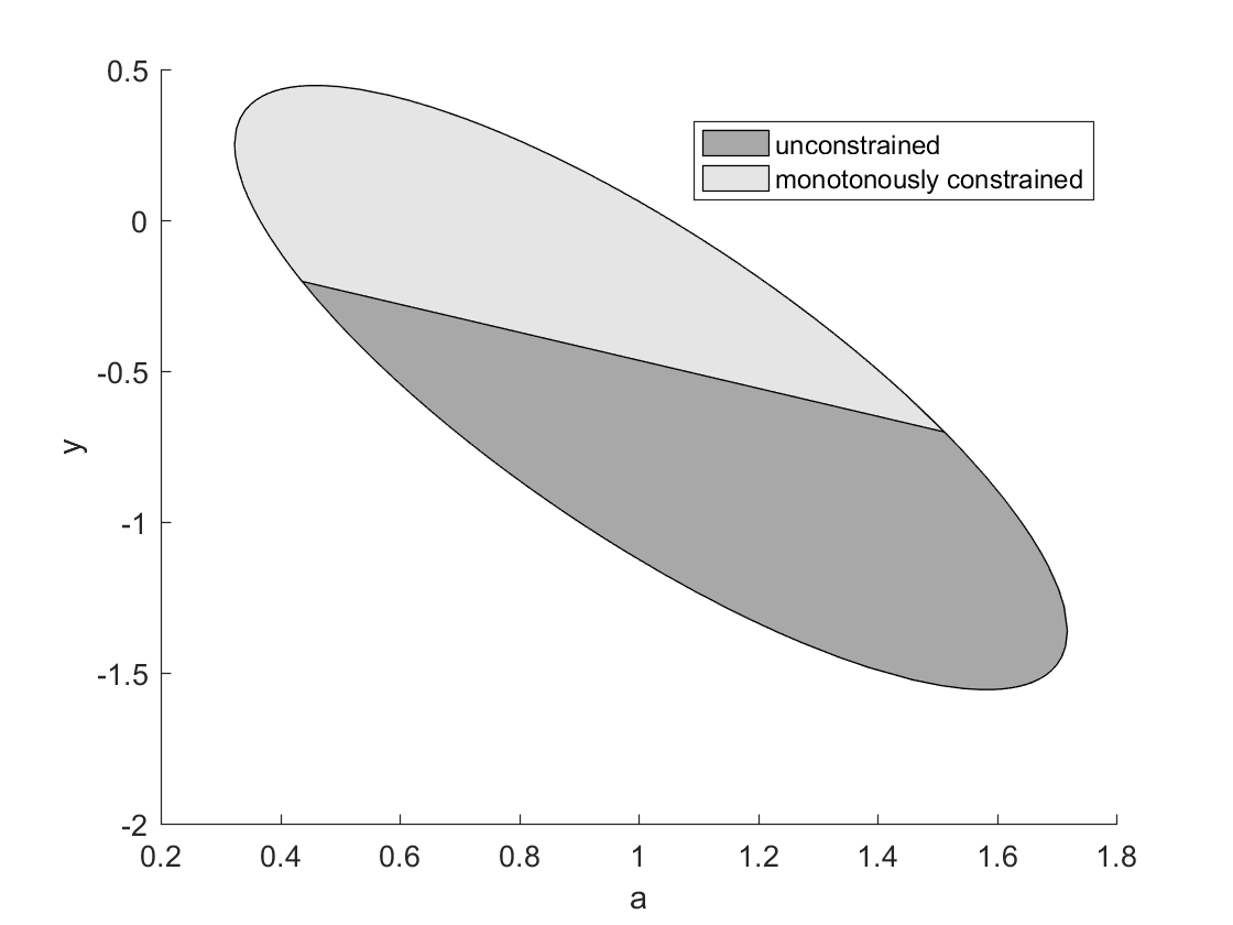
Figure 8.1: Values of $a$ and $b$ for which $p_{a,b}(x)$ in (8.19) has mean squared error less than 250 in the unconstrained and the monotonically-constrained settings

As a sanity check, we plot in Figure 8.2 the fits that we obtain when $(a,b)=(1.6,-1.5)$ and when $(a,b)=(0.6,0)$. Note that the first fit is not monotonous, whereas the second one is, which is what we expect from Figure 8.1.

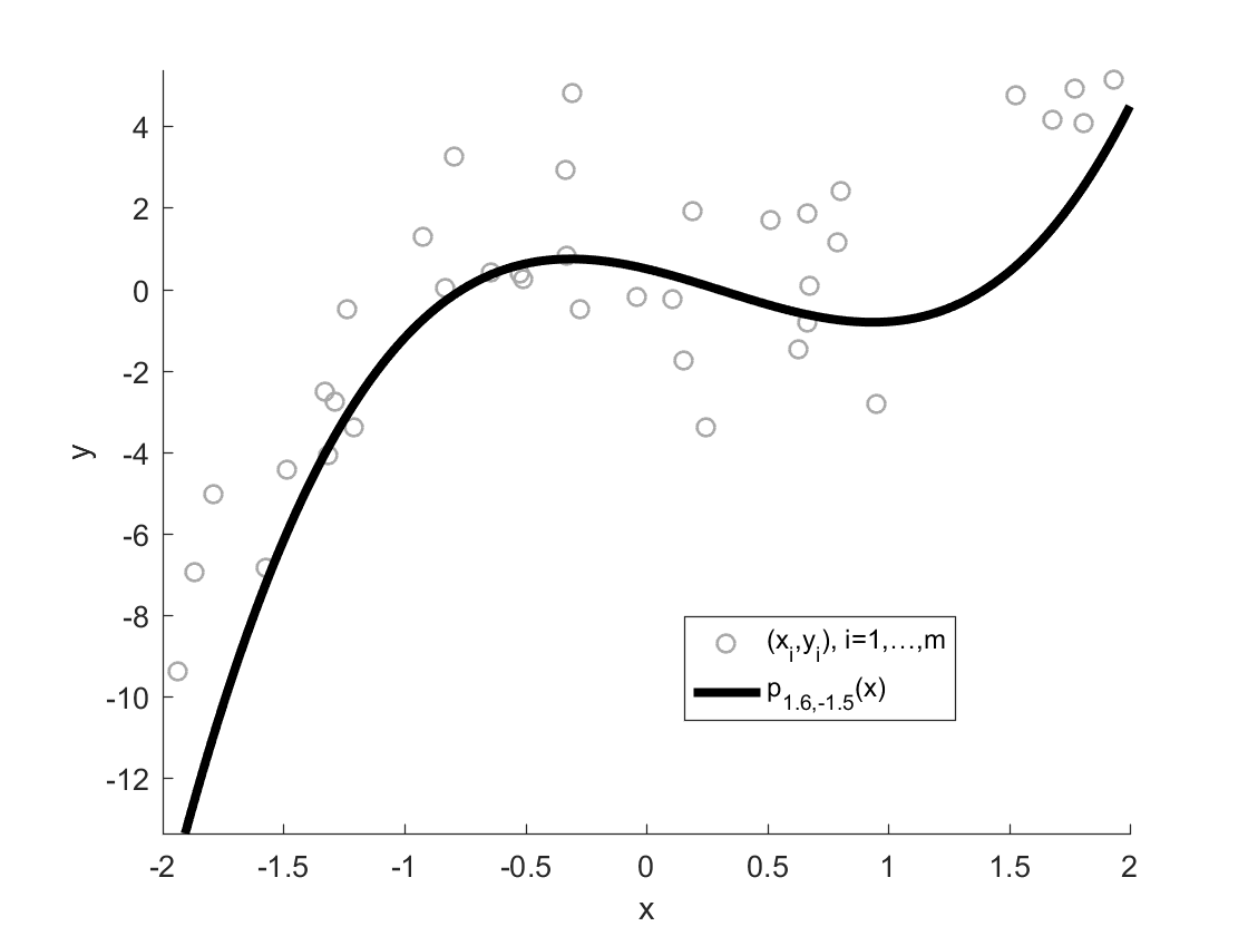
(a) Fit for $(a,b)=(1.6,-1.5)$

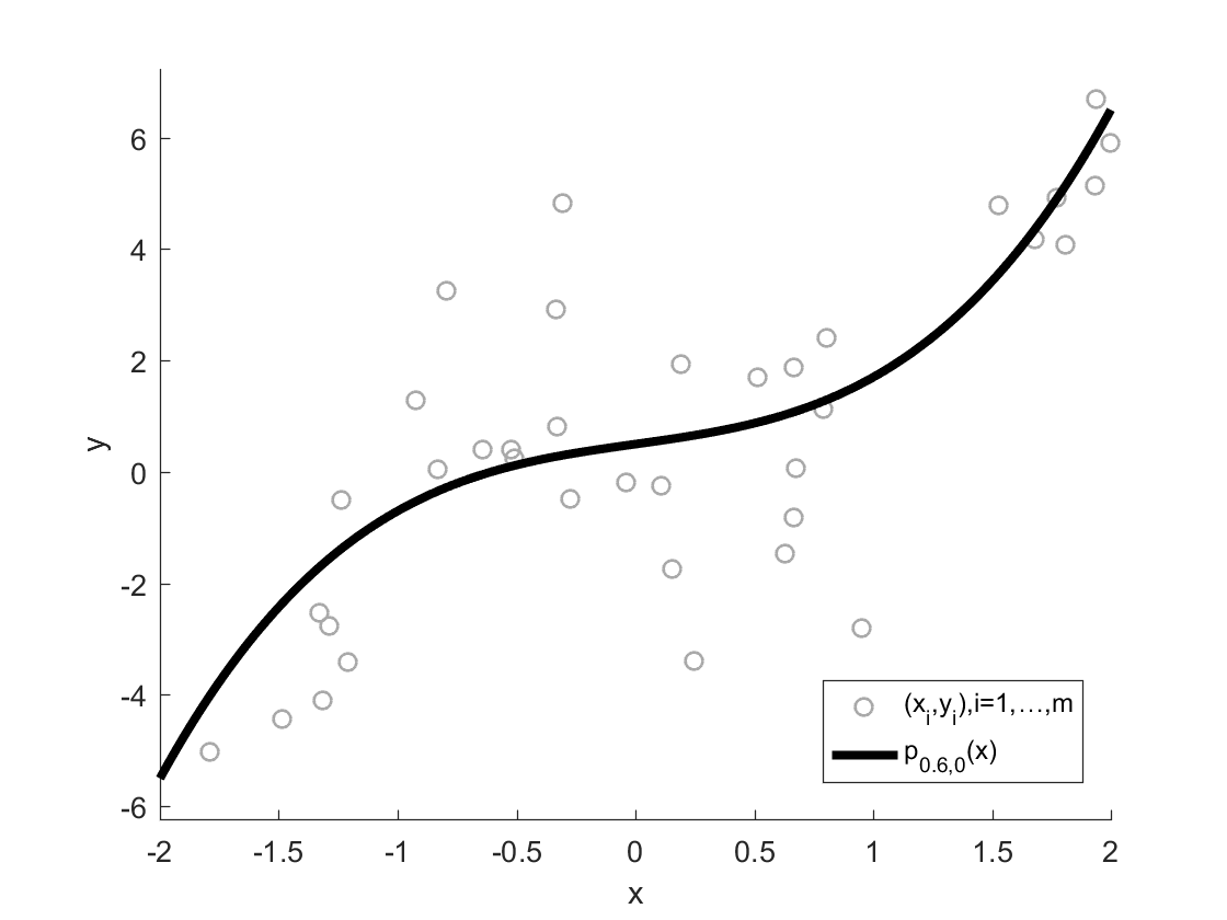
(b) Fit for $(a,b)=(0.6,0)$

Figure 8.2: Plots of the polynomial $p_{a,b}$ in (8.19) for different values of $(a,b)$ in the monotonous case

We now consider the case where we would like to solve (8.15), i.e., where we constrain $p$ to be convex over $B$. We assume that we are searching over the set of separable polynomials of degree $d$. Note here that if $p(x)=\sum_{i=1}^{n}p_{i}(x_{i})$, then $H_{p}(x)$ is a diagonal matrix with diagonal entry $i$ corresponding to $p_{i}^{\prime\prime}(x_{i}).$ Hence, the condition $H_{p}(x)\succeq 0,\forall x\in B$ is equivalent to requiring that $p_{i}^{\prime\prime}(x_{i})\geq 0$, for all $x_{i}\in[b_{i}^{-},b_{i}^{+}]$, $i=1,\ldots,n$. Once again, we use Lemma 8.4.10 to rewrite the previous optimization problem as a semidefinite program. For example, in the case where the degrees of $p_{i}$ are all even and equal to $d=2d^{\prime}$, we get

$$f_{m}\mathrel{\mathop{:}}= \inf_{p\text{ separable of degree }d}\sum_{i=1}^{m}(p(x_{i})-y_{i})^{2}$$

$$\text{s.t. }p_{j}^{\prime\prime}(x_{j})=s_{j}(x)+(x_{j}-b_{j}^{-})(b_{j}^{+}-x_{)}\cdot t_{j}(x),~{}j=1,\ldots,n,$$

$$s_{j}\text{ sos and of degree }\leq 2d^{\prime}-2,~{}t_{j}\text{ sos and of degree }\leq 2d^{\prime}-4.$$

To illustrate these results, we have generated data $(x_{i},y_{i})\in[-2,2]\times\mathbb{R}$ with $i=1,\ldots,40$ which we would like to fit a univariate polynomial $p$ of degree $4$ to. (Note again that the univariate case is a special case of the separable case.) For visualization purposes, we restrict ourselves again to a parametric family of polynomials whose coefficients are indexed by $a$ and $b$:

$$p_{a,b}(x)=\frac{1}{10}x^{4}+a\cdot x^{3}+b\cdot x^{2}-(a+b)\cdot x-\frac{2}{10}.$$ (8.20)

We have plotted in Figure 8.3 the values of $a$ and $b$ for which:

1. $\sum_{i=1}^{40}(p_{a,b}(x_{i})-y_{i})^{2}\leq 7$ in dark gray,

2. $\sum_{i=1}^{40}(p_{a,b}(x_{i})-y_{i})^{2}\leq 7$ and $p_{a,b}$ is convex over $[-2,2]$ in light gray.

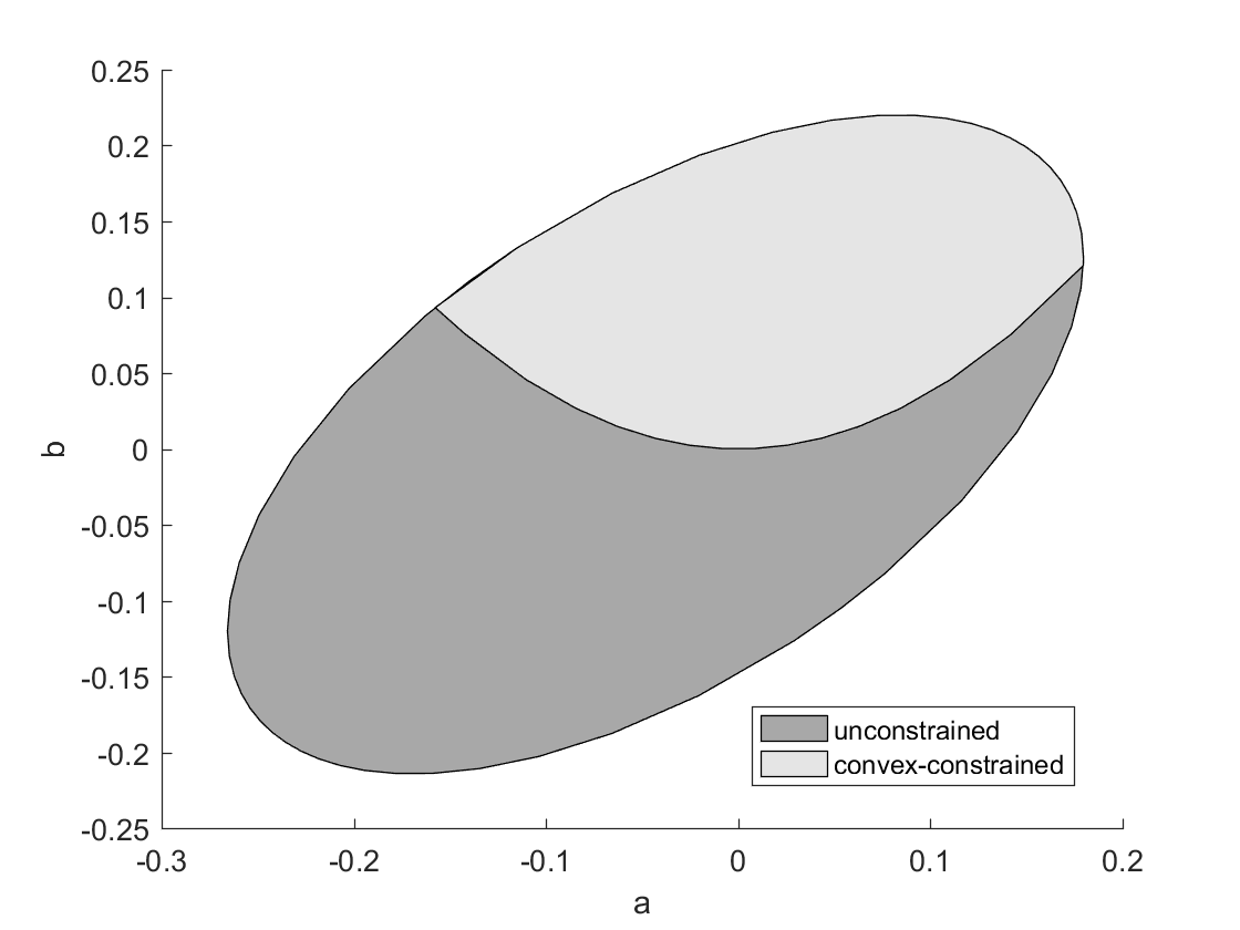
Figure 8.3: Values of $a$ and $b$ for which $p_{a,b}(x)$ in (8.20) has mean squared error less than 7 in the unconstrained and the convexity-constrained settings

As a sanity check, we plot in Figure 8.4 the fits that we obtain when $(a,b)=(-0.2,-0.1)$ and when $(a,b)=(0.15,0.1)$. Note that the first fit is not convex, whereas the second one is, which is what we expect from Figure 8.3.

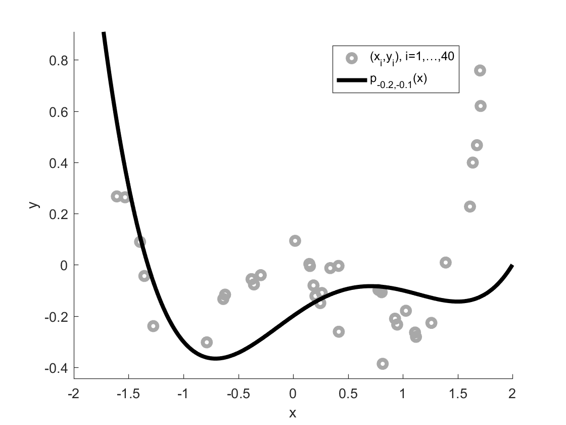
(a) Fit for $(a,b)=(-0.2,-0.1)$

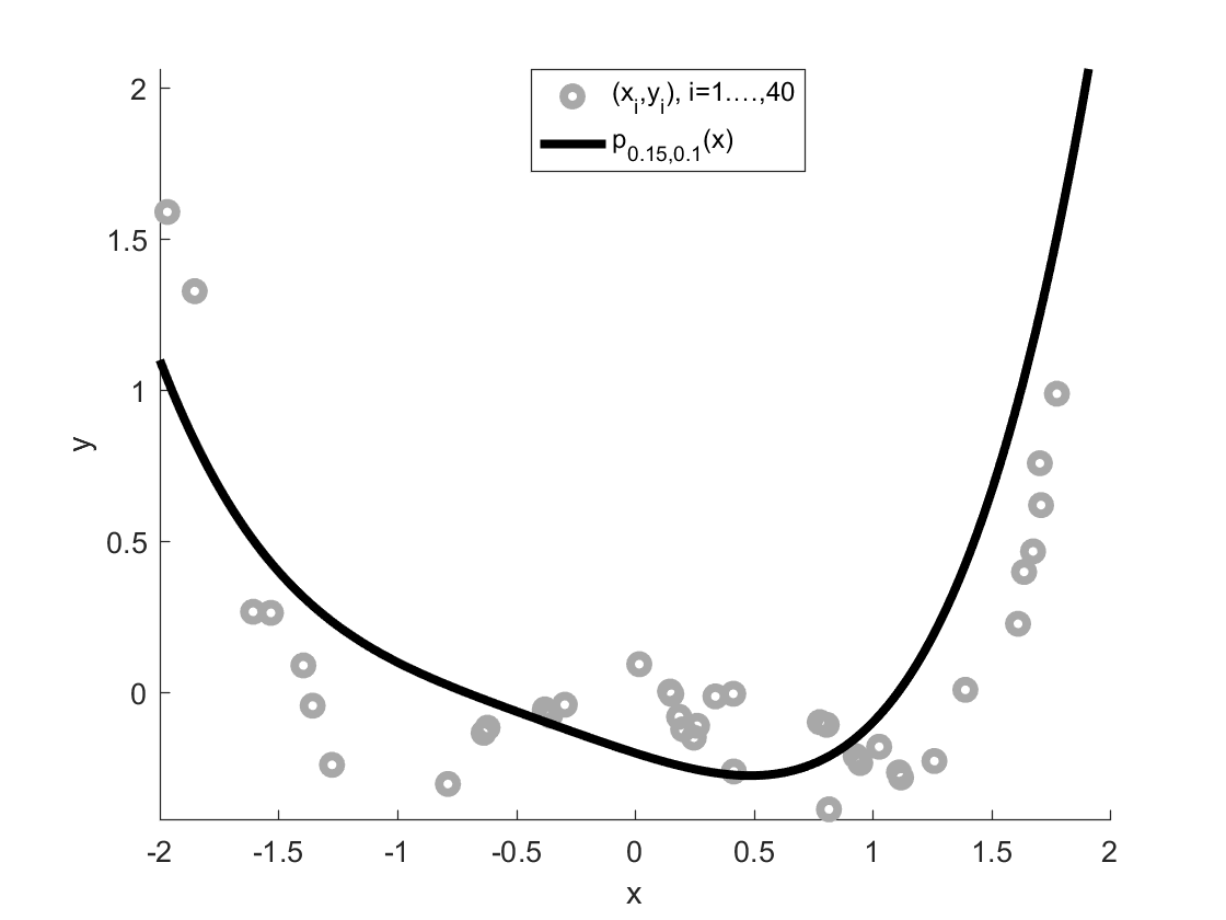
(b) Fit for $(a,b)=(0.15,0.1)$

Figure 8.4: Plot of the polynomial $p_{a,b}$ in (8.20) for different values of $(a,b)$

8.5 Experimental results

We now provide some illustrations of our methods on different datasets. In the first part of this section, we consider synthetic datasets. This will enable us to compare the advantages and limitations of our relaxations in terms of performance metrics such as training and testing accuracy, robustness, flexibility and scalability. In the second part of this section, we look at how our methods perform on real-life datasets.

8.5.1 Synthetic regression problems

For the synthetic experiments, we analyze the performance of 4 different algorithms: UPR, which corresponds to unconstrained polynomial regression, MCPR, which corresponds to polynomial regression with monotonicity constraints, CCPR which corresponds to polynomial regression with convexity constraints, and MCPR+CCPR, which corresponds to polynomial regression with both monotonicity and convexity constraints. The underlying function for this experiment as described in (8.9) is a multivariate exponential:

$$f(x)=e^{\left\|x\right\|_{2}}$$

The function $f:\mathbb{R}^{n}\rightarrow\mathbb{R}$ is monotonically increasing in all directions, thus, it has a monotonicity profile $\rho_{i}=1,\forall i$. Furthermore, $f$ is convex.

Data Generation

We denote by $X$ the feature matrix, i.e., the matrix obtained by concatenating the $m$ feature vectors $x_{i}$ of length $n$. Each column or $X$ corresponds to a feature and each row is an observation of all the $n$ features. Hence, $X$ is an $m\times n$ matrix. For our synthetic datasets, we generate each entry of $X$ uniformly at random in an interval $[b^{-},b^{+}]$, where $b^{-}=0.5$ and $b^{+}=2$. The feature domain in this case is taken to be

$$B=\{x\in\mathbb{R}^{n}~{}|~{}b^{-}\leq x_{i}\leq b^{+},\ i=1,\ldots,n\}.$$

We compute the response variable $y_{i}$ by evaluating $f$ at each column $x_{i}$ of $X$, which we corrupt by some noise, whose scaling $\epsilon$ we vary in order to test for robustness. As a consequence, if we denote by $y$ the $m\times 1$ vector containing $y_{1},\ldots,y_{m}$ and by $f(X)$ the $m\times 1$ vector obtained by applying $f$ to each row of $X$, we have $y=f(X)+\epsilon,$ where $\epsilon$ is a vector with each entry taken to be iid and Gaussian of mean zero and standard deviation $\alpha\sqrt{var(f(X))}$. Here $var(f(X))$ is the variance of the set of random points obtained when varying the input $X$ to $f$ and $\alpha$ is a fixed constant, which we use to parametrize noise (e.g., $\alpha=1$ is low noise, whereas $\alpha=10$ is high noise).

In the following, we wish to fit a polynomial $p$ of degree $d$ to the data, such that the mean squared error (which is a normalization of the least squared error)

$$\frac{1}{m}||p(X)-y||^{2}$$

is minimized.

Comparative performance

One of the biggest drawbacks of unconstrained polynomial regression is the algorithmic instability to noise. Here we want to compare the four algorithms listed above with respect to robustness to noise. To do this, we fit polynomials of varying degrees to the data in both high-noise ($\alpha=10$ as described previously) and low-noise ($\alpha=1$) settings. We then compare the Root Mean Squared Error (RMSE)

$$RMSE(X,y)=\sqrt{\frac{||p(X)-y||^{2}}{m}}$$

on the testing and training samples. The results are given in Figure 8.5. Note that the thin light blue constant line listed as “Reference” is the reference RMSE, i.e., the value obtained when one computes the RMSE for the function $f$ itself.

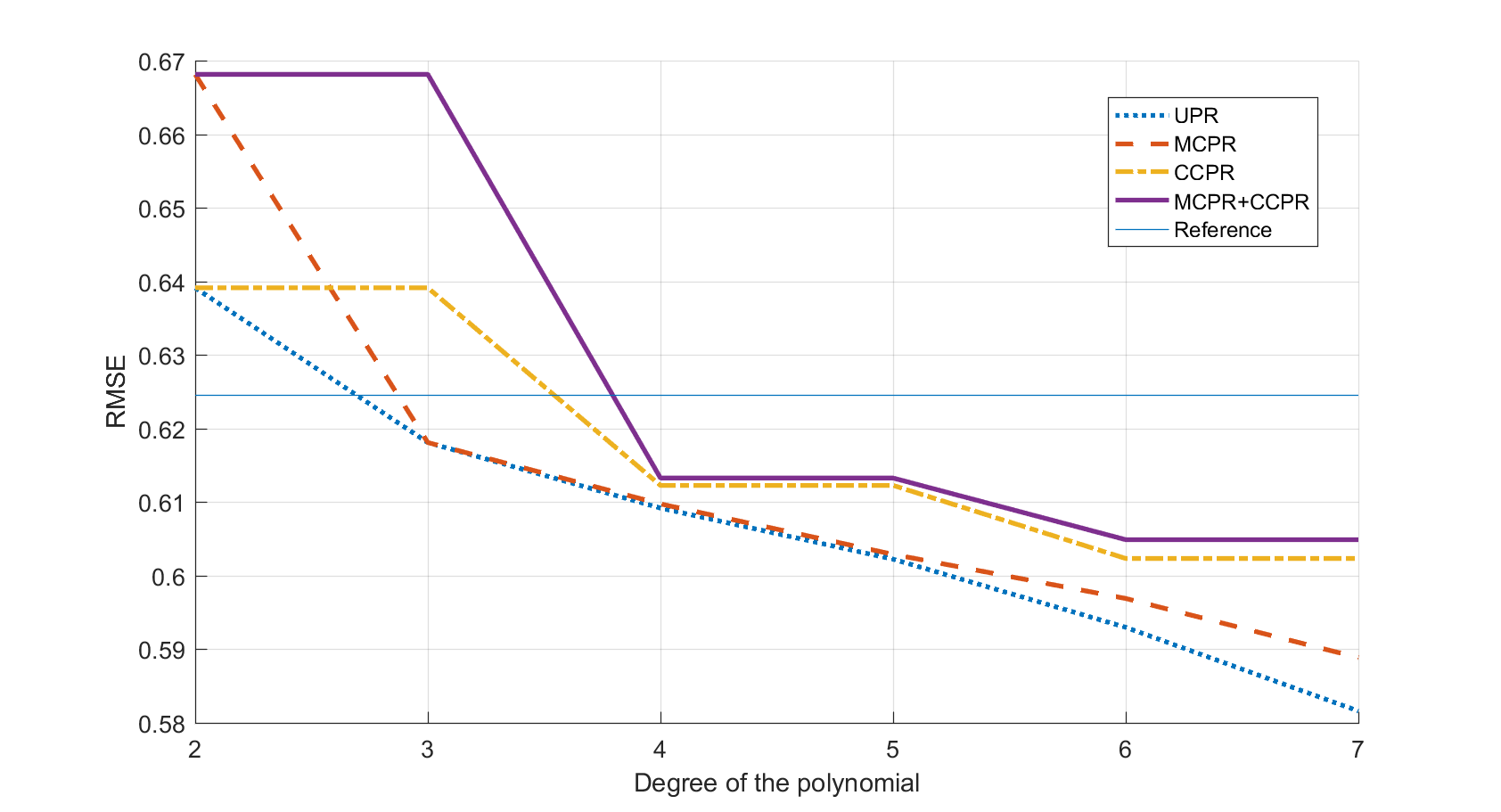
(a) Comparison of RMSE on the training set in a low noise setting

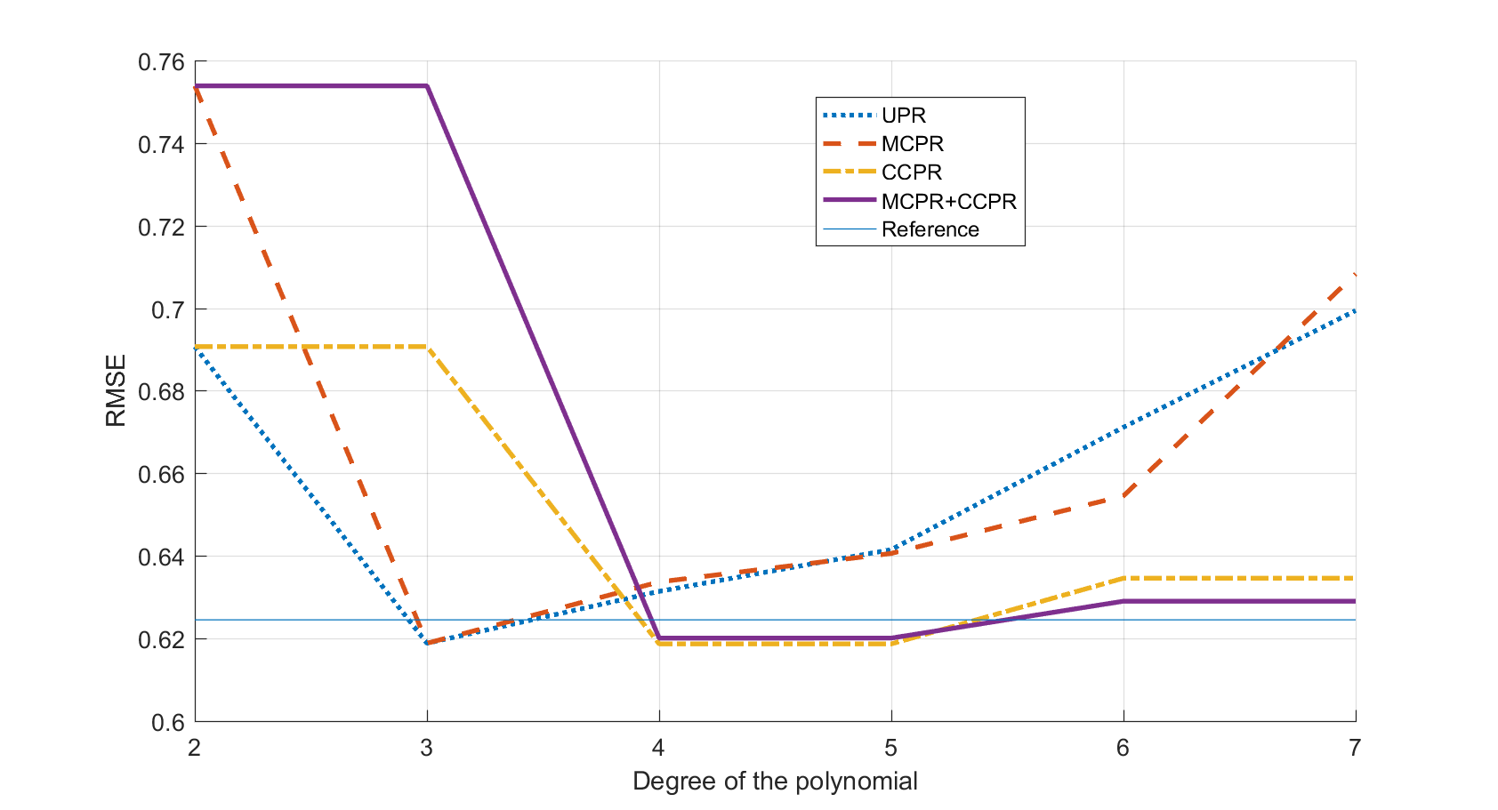
(b) Comparison of RMSE on the testing set in a low noise setting

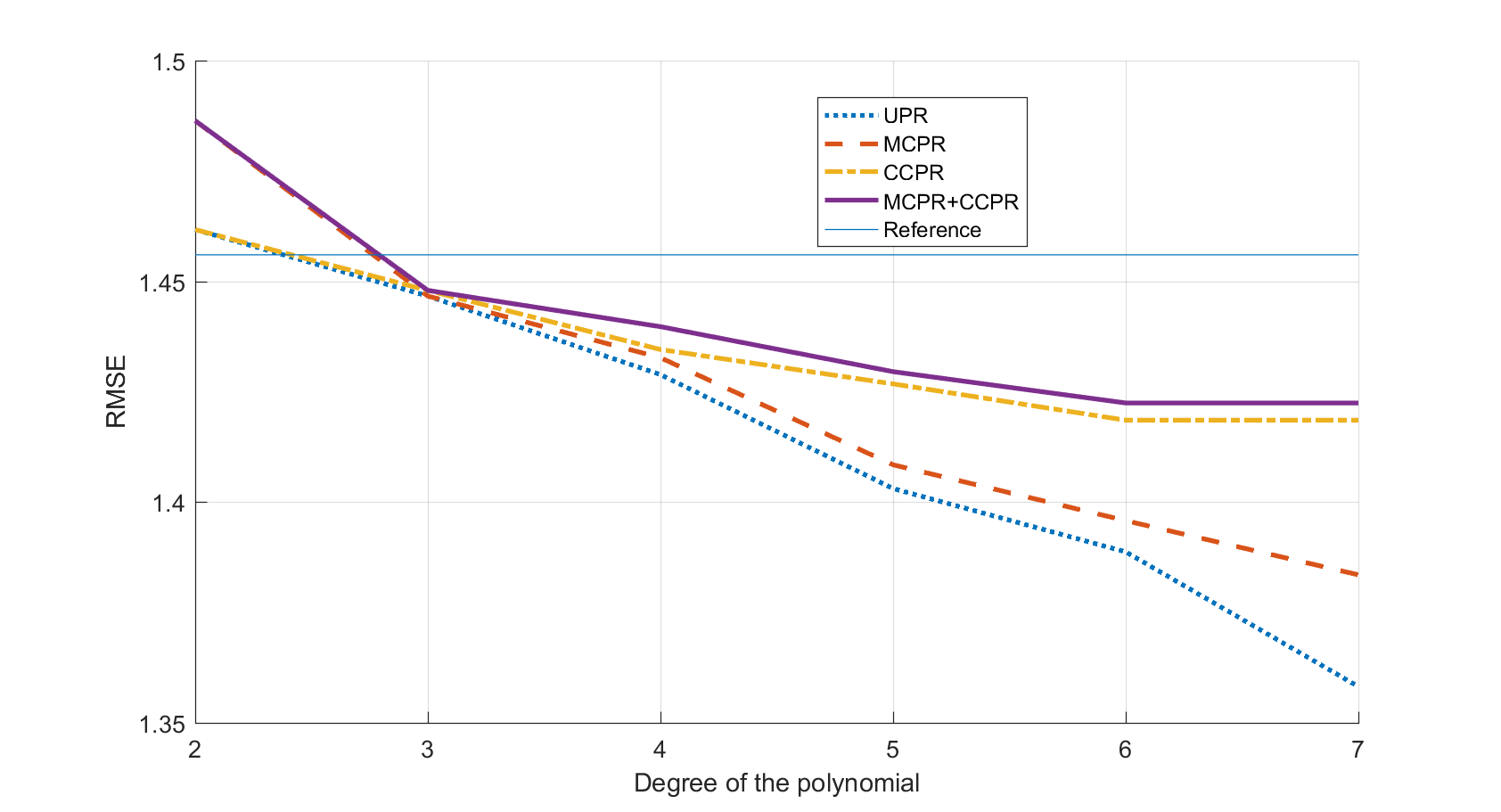
(c) Comparison of RMSE on the training set in a high noise setting

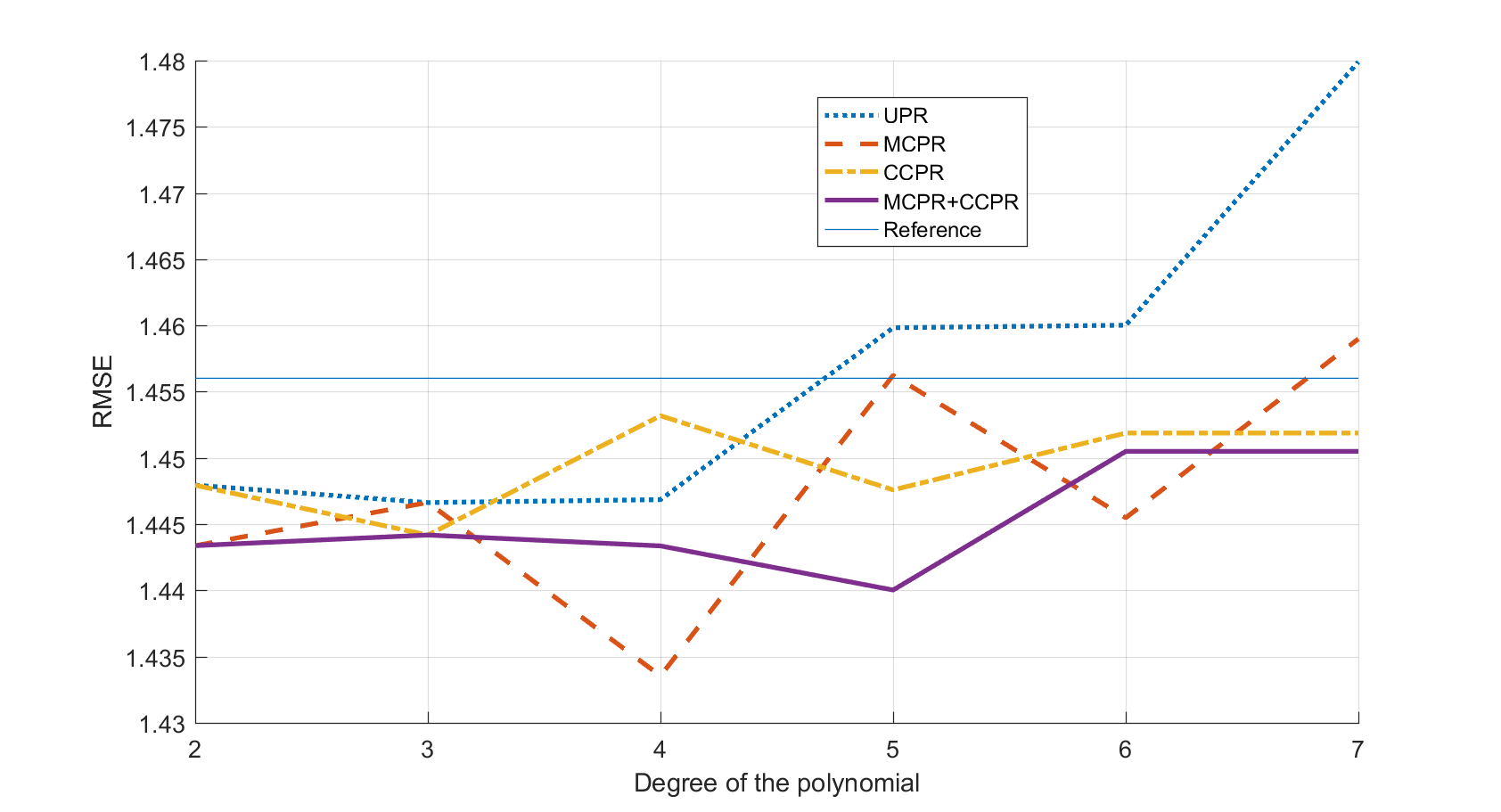
(d) Comparison of RMSE on the testing set in a high noise setting

Figure 8.5: RMSEs of the fitted functions for different noise scaling factors and polynomial degrees

As expected, from Figure 8.5, we see that UPR tends to overfit. This can be observed by comparing the RMSE of UPR to the Reference RMSE: anything below the reference can be considered to be overfitting. Note that for both training sets, and particularly when the degree of the polynomials is high, the data points corresponding to UPR are well below those given by the Reference. Introducing monotonicity or convexity constraints improves both the accuracy on the test data as well as robustness to noise, in the sense that the RMSE of these algorithms remains moderate, even in high noise environments. When both monotonicity and convexity are imposed, the benefits compound. Indeed, MCPR+CCPR has similar performance for both the testing and the training data, and the RMSE obtained with this algorithm is the closest to the reference line. Note that MCPR+CCPR performs well both in low noise as well as high noise settings, which indicates the ability to robustly learn the true underlying distribution.

Lastly we compare qualitatively the robustness of UCR, MCPR, CCPR, and MCPR+CCPR with respect to the true underlying function. The plots in Figure 8.6 are obtained by projecting the 4 fitted functions and the underlying function onto one of the features (this is done by fixing all the other features to some arbitrary values in their range). We consider the case where the polynomials are of degree $4$ and of degree $7$.

(a) Projections of degree 4 fits and the underlying function in a low noise setting

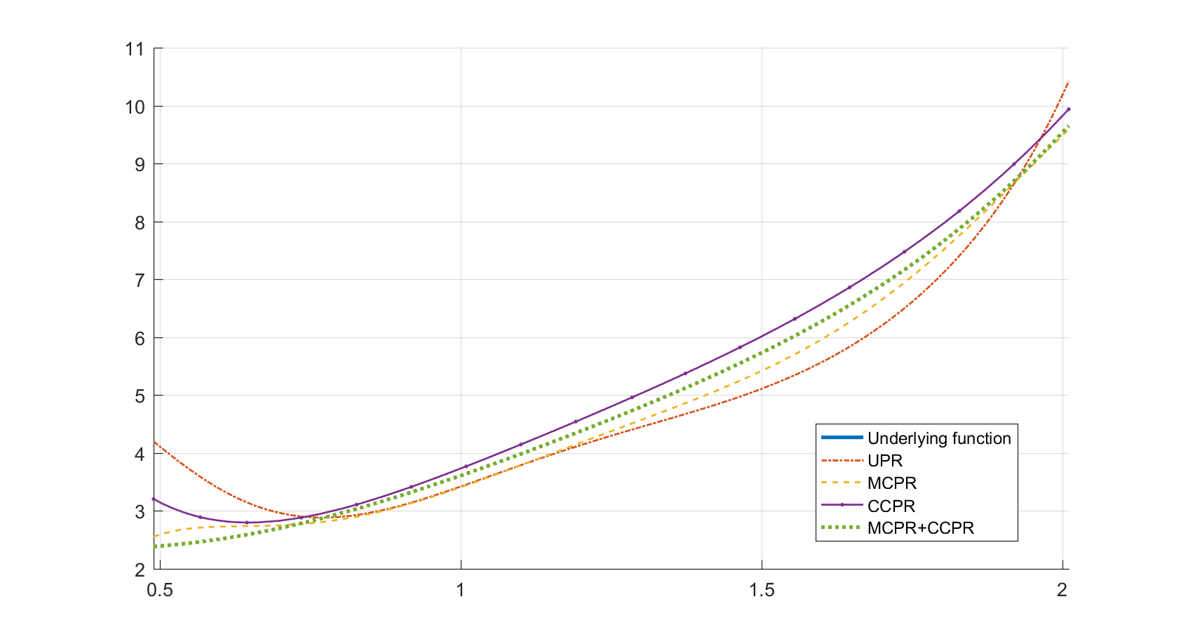
(b) Projections of degree 7 fits and the underlying function in a low noise setting

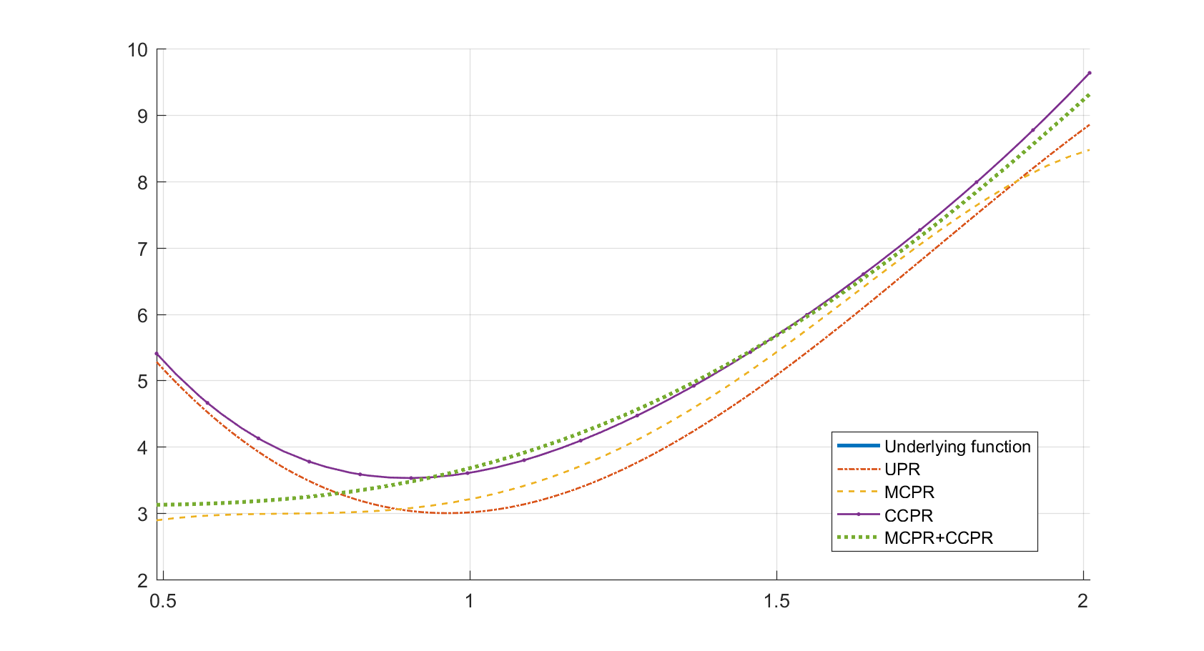
(c) Projections of degree 4 fits and the underlying function in a high noise setting

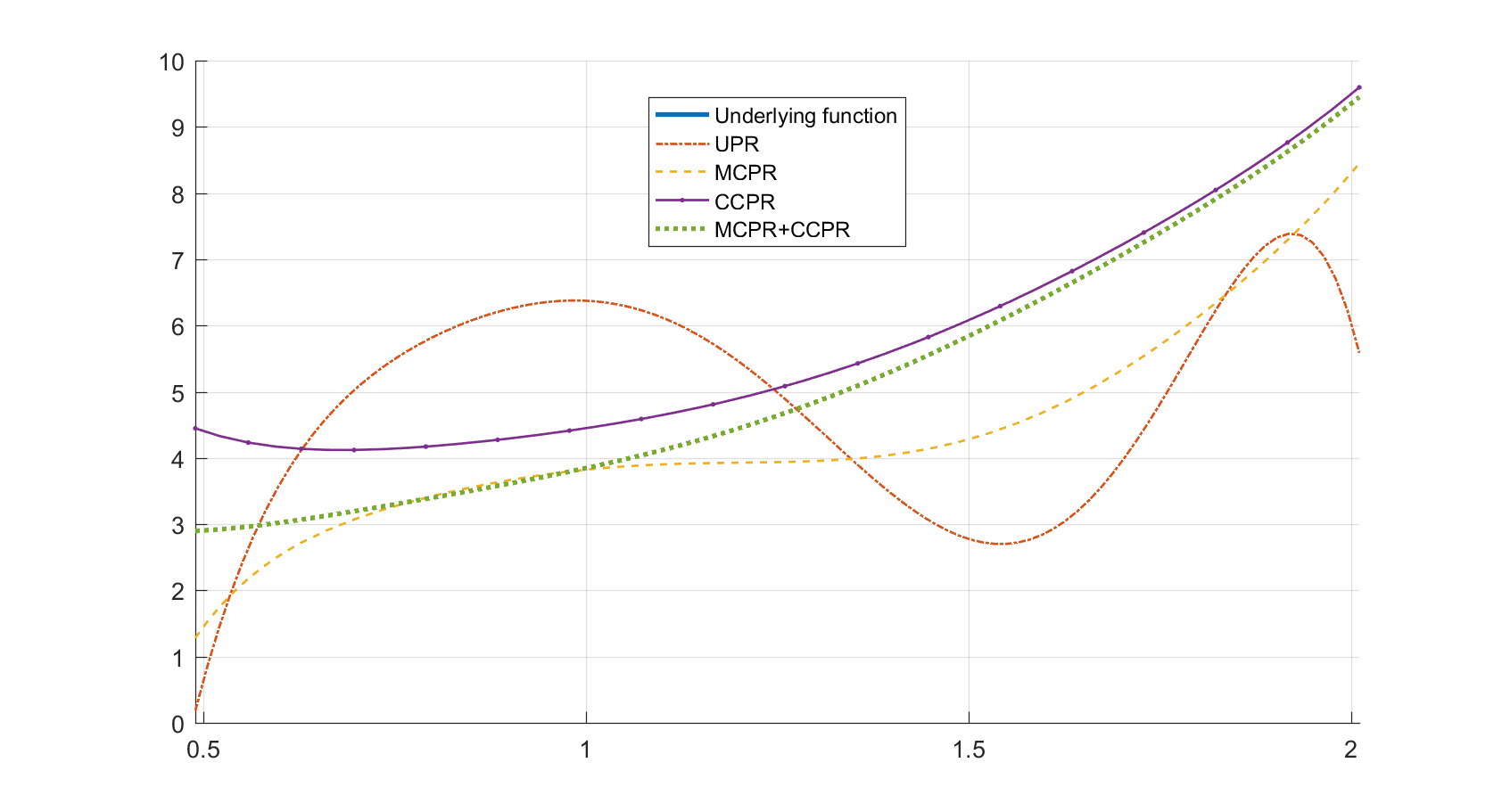
(d) Projections of degree 7 fits and the underlying function in a high noise setting

Figure 8.6: The projection of the fitted functions for different noise scaling factors and polynomial degrees

The results obtained confirm our previous observations. First, UPR tends to overfit, particularly when the noise scaling factor is high and when the degree of the polynomial fit is large (this is because, as the degree increases, the polynomials gain in expressiveness). Having monotonicity and convexity constraints proves to be a very efficient way of regularizing the polynomial fit, even in high noise settings: the fits obtained are very close to the true function. Furthermore, though their performance does deteriorate slightly in the high noise and high degree regime, the overall shape of the projection stays close to that of the underlying function, and that of lower degrees. This in contrast to the unconstrained fit whose shape is very unstable when the degree and the noise varies.

8.5.2 Applications to real regression problems

In this section we present two applications of our methods to real datasets. Our first example uses monotonically constrained polynomial regression (MPCR) to predict interest rates for personal loans. The second example is a hybrid regression setting with a mixture of monotonicity and convexity constraints which is used to predict weekly wages from a set of features.

8.5.3 Predicting interest rates for personal loans

In this subsection, we study data for loans issued between the years 2007-2011 by Lending Club [118]. We decided to focus on the particular category of home loans so as to avoid having to deal with categorical variables such as loan type. The updated dataset has $N=3707$ observations and 32 numerical features. Though the MCPR algorithm has run time polynomial in the number of features, we encounter issues with memory for too large a number of features. Hence, some data preprocessing is necessary to reduce the number of features. This was done by eliminating highly correlated covariates and running some canonical feature selection procedures. In the end, we consider six features. The response variable in this case is the interest rate on home loans. The features along with their monotonicity signs and their descriptions are presented below:

• dti:+1 - Ratio of the borrower’s total monthly debt payments an the self-reported monthly income. A borrower with high dti is perceived to be riskier, which typically corresponds to higher interest rates.

• delinq_2yrs:+1 - The number of past-due delinquencies in the past 2 years. The interest rate is monotonically increasing with respect to the number of delinquencies.

• pub_rec:+1 - Number of derogatory public records. The interest rate is monotonically increasing with respect to this feature.

• out_prncp:+1 - Remaining outstanding principal. This feature has a monotonically increasing relationship with the interest rate.

• total_rec_prncp:-1 - Principal received to date with a monotonically decreasing dependency.

• total_rec_int:-1 - Interest received to date. The interest rate is monotonically decreasing with respect to this feature.

We compute the average RMSE for testing and training sets through a 10-fold cross validation. We compare in Figure 8.7 the results for fitting polynomials of different degrees in both the unconstrained and monotonically constrained settings.

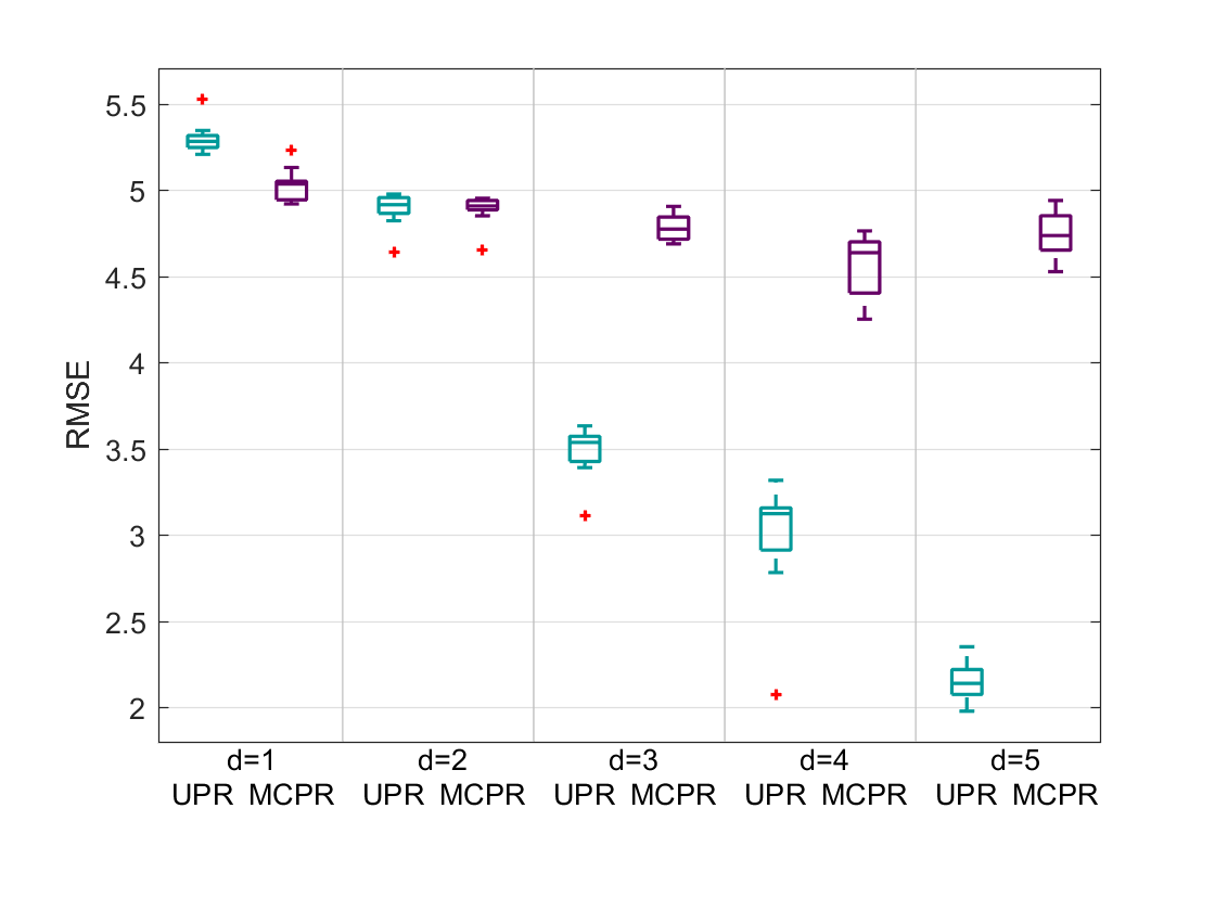
(a) Values taken by the RMSE on training data

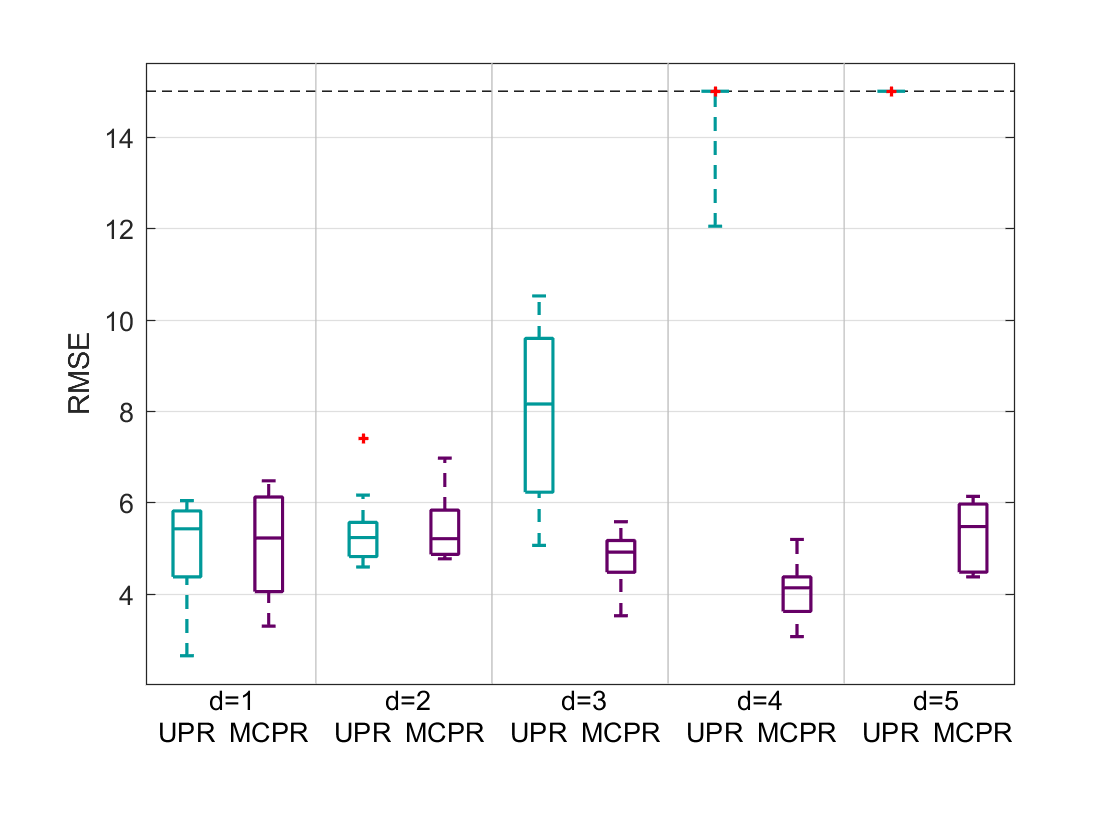
(b) Values taken by the RMSE on testing data

Figure 8.7: Comparative performance of testing and training sets for 10 fold cross validation.

The best performance was achieved by a degree 4, monotonically constrained polynomial regression with average RMSE of $4.09$ and standard error of $0.20$. Already for degree $5$, the unconstrained regression runs into numerical problems as it becomes rank deficient, i.e., the number of coefficients that needs to be determined is larger than the number of data points. Therefore, monotonicity constraints can be an efficient way of ensuring robustness in settings where the number of datapoints is relatively small, but the relationship between the covariates is complex.

8.5.4 Predicting weekly wages

In this section, we analyze data from the 1988 Current Population Survey. This data is freely available under the name ex1029 in the Sleuth2 R package [163]. The data contains $N=25361$ observations and 2 numerical features: years of experience and years of education. We expect wages to increase with respect to years of education and be concave with respect to years of experience. We compare the performance of this hybrid constrained regression problem with the unconstrained case, as well as the CAP algorithm proposed by Hannah [84]. Similarly to the previous example we compute the RMSEs with 10-fold cross validation. In addition we time our algorithm in order to compare the runtimes with the CAP algorithm. The results are presented in Figure 8.8.

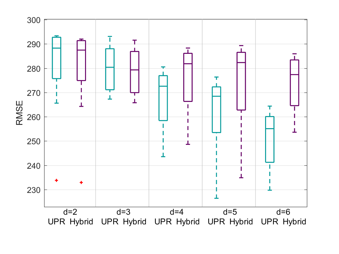
(a) Values taken by the RMSE on training data

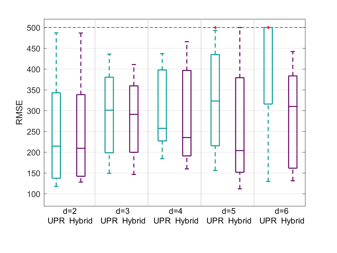
(b) Values taken by the RMSE on testing data

Figure 8.8: Comparative performance of testing and training sets for 10 fold cross validation.

The best performing algorithm is the monotonically and convexly constrained degree 2 polynomial with average test RMSE: $250.0$ and standard error $39.2$. The algorithm with the smallest standard error, therefore the one with the most consistent performance is the degree 3 hybrid polynomial with test RMSE: $285.0\pm 29.9$. In comparison, the CAP and Fast CAP algorithm have test RMSE: $385.7\pm 20.8$. Our algorithm does not only perform better in terms of RMSE, it also has a better runtime performance. For the degree 2 hybrid regression, the run time is $0.24\pm 0.01$ seconds, and for degree 3, the hybrid regresion runtime is $0.26\pm 0.01$ seconds. In contrast, the CAP algorithm takes $12.8\pm 0.8$ seconds and the Fast CAP algorithm takes $1.9\pm 0.2$ seconds.

References

- [1] A. A. Ahmadi. Algebraic relaxations and hardness results in polynomial optimization and Lyapunov analysis. PhD thesis, Massachusetts Institute of Technology, September 2011. Available at http://aaa.princeton.edu/publications.
- [2] A. A. Ahmadi. On the difficulty of deciding asymptotic stability of cubic homogeneous vector fields. In Proceedings of the American Control Conference, 2012.
- [3] A. A. Ahmadi and R. Jungers. SOS-convex Lyapunov functions with applications to nonlinear switched systems. In Proceedings of the IEEE Conference on Decision and Control, 2013.
- [4] A. A. Ahmadi, R. Jungers, P. A. Parrilo, and M. Roozbehani. Analysis of the joint spectral radius via lyapunov functions on path-complete graphs. In Proceedings of the 14th international conference on Hybrid systems: computation and control, pages 13–22. ACM, 2011.
- [5] A. A. Ahmadi and R. M. Jungers. Lower bounds on complexity of Lyapunov functions for switched linear systems. Nonlinear Analysis: Hybrid Systems, 21:118–129, 2016.
- [6] A. A. Ahmadi and R. M. Jungers. SOS-convex Lyapunov functions and stability of nonlinear difference inclusions. 2017. To appear. Available at arXiv:1803.02070.
- [7] A. A. Ahmadi and A. Majumdar. DSOS and SDSOS optimization: LP and SOCP-based alternatives to sum of squares optimization. In Proceedings of the 48th Annual Conference on Information Sciences and Systems. Princeton University, 2014.
- [8] A. A. Ahmadi and A. Majumdar. Some applications of polynomial optimization in operations research and real-time decision making. Optimization Letters, 10(4):709–729, 2016.
- [9] A. A. Ahmadi and A. Majumdar. DSOS and SDSOS: more tractable alternatives to sum of squares and semidefinite optimization. To appear. Available at arXiv:1706.02586, 2017.
- [10] A. A. Ahmadi, A. Olshevsky, P. A. Parrilo, and J. N. Tsitsiklis. NP-hardness of deciding convexity of quartic polynomials and related problems. Mathematical Programming, 137(1-2):453–476, 2013.
- [11] A. A. Ahmadi and P. A. Parrilo. A convex polynomial that is not sos-convex. Mathematical Programming, 135(1-2):275–292, 2012.
- [12] A. A. Ahmadi and P. A. Parrilo. A complete characterization of the gap between convexity and SOS-convexity. SIAM Journal on Optimization, 23(2):811–833, 2013.
- [13] A. A. Ahmadi and P. A. Parrilo. Towards scalable algorithms with formal guarantees for lyapunov analysis of control systems via algebraic optimization. In Decision and Control (CDC), 2014 IEEE 53rd Annual Conference on, pages 2272–2281. IEEE, 2014.
- [14] Y. Ait-Sahalia and J. Duarte. Nonparametric option pricing under shape restrictions. Journal of Econometrics, 116(1-2):9–47, 2003.
- [15] F. Alizadeh and D. Goldfarb. Second-order cone programming. Mathematical Programming, 95(1):3–51, 2003.
- [16] A. Alvarado, G. Scutari, and J.S. Pang. A new decomposition method for multiuser DC-programming and its applications. Signal Processing, IEEE Transactions on, 62(11):2984–2998, 2014.
- [17] A. Argyriou, R. Hauser, C. A. Micchelli, and M. Pontil. A DC-programming algorithm for kernel selection. In Proceedings of the 23rd international conference on Machine learning, pages 41–48. ACM, 2006.
- [18] E. Artin. Über die Zerlegung Definiter Funktionen in Quadrate. Hamb. Abh., 5:100–115, 1927.
- [19] Emil Artin. Über die Zerlegung definiter Funktionen in Quadrate. In Abhandlungen aus dem mathematischen Seminar der Universität Hamburg, volume 5, pages 100–115. Springer, 1927.
- [20] G. Averkov. Constructive proofs of some Positivstellensätze for compact semialgebraic subsets of . Journal of Optimization Theory and Applications, 158(2):410–418, 2013.
- [21] F. Bach, R. Jenatton, J. Mairal, G. Obozinski, et al. Optimization with sparsity-inducing penalties. Foundations and Trends in Machine Learning, 4(1):1–106, 2012.
- [22] G. Barker and D. Carlson. Cones of diagonally dominant matrices. Pacific Journal of Mathematics, 57(1):15–32, 1975.
- [23] C. Barnhart, E. L. Johnson, G. L. Nemhauser, M. W. P. Savelsbergh, and Pamela. H. Vance. Branch-and-price: Column generation for solving huge integer programs. Operations research, 46(3):316–329, 1998.
- [24] A. Barvinok. Approximating a norm by a polynomial. In Geometric Aspects of Functional Analysis, pages 20–26. Springer, 2003.
- [25] A. Barvinok and E. Veomett. The computational complexity of convex bodies. arXiv preprint math/0610325, 2006.
- [26] A. Ben-Tal and A. Nemirovski. On polyhedral approximations of the second-order cone. Mathematics of Operations Research, 26(2):193–205, 2001.
- [27] H.P. Benson. Concave Minimization: Theory, Applications and Algorithms. In R. Horst and P.M. Pardalos, editors, Handbook of Global Optimization, chapter 3, pages 43–148. Springer, Boston, MA, 1995.
- [28] D. Bertsimas, R. M. Freund, and X. A. Sun. An accelerated first-order method for solving SOS relaxations of unconstrained polynomial optimization problems. Optimization Methods and Software, 28(3):424–441, 2013.
- [29] R. Bhatia. Matrix Analysis, volume 169. Springer Science & Business Media, 2013.
- [30] G. Blekherman, P. A. Parrilo, and R. R. Thomas. Semidefinite Optimization and Convex Algebraic Geometry. SIAM, 2012.
- [31] V. D. Blondel and J. N. Tsitsiklis. The boundedness of all products of a pair of matrices is undecidable. Systems and Control Letters, 41:135–140, 2000.
- [32] I. M. Bomze and E. de Klerk. Solving standard quadratic optimization problems via linear, semidefinite and copositive programming. Journal of Global Optimization, 24(2):163–185, 2002.
- [33] I.M. Bomze and M. Locatelli. Undominated DC decompositions of quadratic functions and applications to branch-and-bound approaches. Computational Optimization and Applications, 28(2):227–245, 2004.
- [34] E. Boros, P.L. Hammer, and G. Tavares. Local search heuristics for quadratic unconstrained binary optimization (qubo). Journal of Heuristics, 13(2):99–132, 2007.
- [35] S. Boyd and L. Vandenberghe. Convex Optimization. Cambridge University Press, 2004.
- [36] L. Breiman, J. Friedman, C. J. Stone, and R. 0.A Olshen. Classification and regression trees. CRC press, 1984.
- [37] S. Burer. Copositive programming. In Handbook on semidefinite, conic and polynomial optimization, pages 201–218. Springer, 2012.
- [38] S. Burer, K. M. Anstreicher, and M. Dür. The difference between 5 5 doubly nonnegative and completely positive matrices. Linear Algebra and its Applications, 431(9):1539–1552, 2009.
- [39] V. Chandrasekaran, B. Recht, P. A. Parrilo, and A. S. Willsky. The convex geometry of linear inverse problems. Foundations of Computational Mathematics, 12(6):805–849, 2012.
- [40] O. Chapelle, C. B. Do, C. H. Teo, Q. V. Le, and A. J. Smola. Tighter bounds for structured estimation. In Advances in Neural Information Processing Systems, pages 281–288, 2009.
- [41] V. Charpentier, S. Adriaenssens, F. Meggers, and O. Baverel. Comfort driven optimization and control for adaptive shading applications. Building Information and Research, 2017.
- [42] Y. Chen and R. J. Samworth. Generalized additive and index models with shape constraints. Journal of the Royal Statistical Society: Series B (Statistical Methodology), 78(4):729–754, 2016.
- [43] H. A. Chipman, E. I. George, R. E. McCulloch, and T. S. Shively. High-dimensional nonparametric monotone function estimation using BART. arXiv preprint arXiv:1612.01619, 2016.
- [44] M. D. Choi and T. Y. Lam. Extremal positive semidefinite forms. Math. Ann., 231:1–18, 1977.
- [45] E. K. P. Chong and S. H. Zak. An Introduction to Optimization, volume 76. John Wiley & Sons, 2013.
- [46] D. Cifuentes and P. A. Parrilo. Exploiting chordal structure in polynomial ideals: a Gröbner bases approach. SIAM Journal on Discrete Mathematics, 30(3):1534–1570, 2016.
- [47] CPLEX. V12. 4: Users manual for CPLEX. International Business Machines Corporation, 46(53):157.
- [48] F. Dabbene and D. Henrion. Set approximation via minimum-volume polynomial sublevel sets. Proceedings of the European Control Conference, Zurich, Switzerland, July 2013.
- [49] F. Dabbene, D. Henrion, and C. Lagoa. Simple approximations of semialgebraic sets and their applications to control. Automatica, 78:110–118, 2017.
- [50] H. Dai, A. Majumdar, and R. Tedrake. Synthesis and optimization of force closure grasps via sequential semidefinite programming. In International Symposium on Robotics Research. Citeseer, 2015.
- [51] H. Daniels and M. Velikova. Monotone and partially monotone neural networks. IEEE Transactions on Neural Networks, 21(6):906–917, 2010.
- [52] S. Dash. A note on QUBO instances defined on Chimera graphs. arXiv preprint arXiv:1306.1202, 2013.
- [53] E. de Klerk and M. Laurent. On the Lasserre hierarchy of semidefinite programming relaxations of convex polynomial optimization problems. Available at http://www.optimization-online.org/DB-FILE/2010/11/2800.pdf, 2010.
- [54] E. de Klerk, M. Laurent, and P. Parrilo. On the equivalence of algebraic approaches to the minimization of forms on the simplex. Positive Polynomials in Control, pages 580–580, 2005.
- [55] E. de Klerk and D. Pasechnik. Approximation of the stability number of a graph via copositive programming. SIAM Journal on Optimization, 12(4):875–892, 2002.
- [56] E. De Klerk and R. Sotirov. Exploiting group symmetry in semidefinite programming relaxations of the quadratic assignment problem. Mathematical Programming, 122(2):225, 2010.
- [57] J. A. de Loera and F. Santos. An effective version of Pólya’s theorem on positive definite forms. Journal of Pure and Applied Algebra, 108(3):231–240, 1996.
- [58] G. Desaulniers, J. Desrosiers, and M. M. Solomon. Column generation, volume 5. Springer Science & Business Media, 2006.
- [59] P.J.C. Dickinson and L. Gijben. On the computational complexity of membership problems for the completely positive cone and its dual. Available at http://www.optimization-online.org/DB-FILE/2011/05/3041.pdf, 2011.
- [60] C. Dugas, Y. Bengio, F. Bélisle, C. Nadeau, and R. Garcia. Incorporating second-order functional knowledge for better option pricing. Advances in neural information processing systems, pages 472–478, 2001.
- [61] C. Dugas, Y. Bengio, F. Bélisle, C. Nadeau, and R. Garcia. Incorporating functional knowledge in neural networks. Journal of Machine Learning Research, 10(Jun):1239–1262, 2009.
- [62] M. Dür. A parametric characterization of local optimality. Mathematical Methods of Operations Research, 57(1):101–109, 2003.
- [63] CD Elphinstone. A target distribution model for nonparametric density estimation. Communications in Statistics-Theory and Methods, 12(2):161–198, 1983.
- [64] C. Ericson. Real-time Collision Detection. Morgan Kaufmann Series in Interactive 3-D Technology, 2004.
- [65] A. Fellhauer. Approximation of smooth functions using Bernstein polynomials in multiple variables. arXiv preprint arXiv:1609.01940, 2016.
- [66] C.A. Floudas and P.M. Pardalos. Optimization in computational chemistry and molecular biology: local and global approaches, volume 40. Springer Science & Business Media, 2013.
- [67] G.B. Folland. How to integrate a polynomial over a sphere. American Mathematical Monthly, pages 446–448, 2001.
- [68] Y. Freund, R. Schapire, and N. Abe. A short introduction to boosting. Journal-Japanese Society For Artificial Intelligence, 14(771-780):1612, 1999.
- [69] J. H. Friedman. Greedy function approximation: a gradient boosting machine. Annals of statistics, pages 1189–1232, 2001.
- [70] G. Fung and O.L. Mangasarian. Semi-supervised support vector machines for unlabeled data classification. Optimization methods and software, 15(1):29–44, 2001.
- [71] M. R. Garey and D. S. Johnson. Computers and Intractability. W. H. Freeman and Co., San Francisco, Calif., 1979.
- [72] K. Gatermann and P. A. Parrilo. Symmetry groups, semidefinite programs, and sums of squares. Journal of Pure and Applied Algebra, 192:95–128, 2004.
- [73] S. A. Gershgorin. Über die Abgrenzung der Eigenwerte einer Matrix. Bulletin de l’Académie des Sciences de l’URSS. Classe des sciences mathématiques et na, (6):749–754, 1931.
- [74] M. C. Golumbic. Algorithmic graph theory and its applications. In Graph Theory, Combinatorics and Algorithms, pages 41–62. Springer, 2005.
- [75] S. Gottschalk, M. C. Lin, and D. Manocha. Obbtree: A hierarchical structure for rapid interference detection. In Proceedings of the 23rd annual conference on Computer graphics and interactive techniques, pages 171–180. ACM, 1996.
- [76] N. Gulpinar, L. T. Hoai An, and M. Moeini. Robust investment strategies with discrete asset choice constraints using DC programming. Optimization, 59(1):45–62, 2010.
- [77] A. Guntuboyina and B. Sen. Global risk bounds and adaptation in univariate convex regression. Probability Theory and Related Fields, 163(1-2):379–411, 2015.
- [78] M. R. Gupta, A. Cotter, J. Pfeifer, K. Voevodski, K. Canini, A. Mangylov, W. Moczydlowski, and A. Van Esbroeck. Monotonic calibrated interpolated look-up tables. Journal of Machine Learning Research, 17(109):1–47, 2016.
- [79] Gurobi optimizer reference manual. URL: http://www. gurobi. com, 2012.
- [80] N. Gvozdenović and M. Laurent. Semidefinite bounds for the stability number of a graph via sums of squares of polynomials. Mathematical Programming, 110(1):145–173, 2007.
- [81] W. Habicht. Über die Zerlegung strikte definiter Formen in Quadrate. Commentarii Mathematici Helvetici, 12(1):317–322, 1939.
- [82] D. Handelman. Representing polynomials by positive linear functions on compact convex polyhedra. Pacific Journal of Mathematics, 132(1):35–62, 1988.
- [83] L. Hannah and D. Dunson. Ensemble methods for convex regression with applications to geometric programming based circuit design. arXiv preprint arXiv:1206.4645, 2012.
- [84] L. A. Hannah and D. B. Dunson. Multivariate convex regression with adaptive partitioning. The Journal of Machine Learning Research, 14(1):3261–3294, 2013.
- [85] P. Hartman. On functions representable as a difference of convex functions. Pacific J. Math, 9(3):707–713, 1959.
- [86] J. Håstad. Clique is hard to approximate within . In Proceedings of the 37th Annual Symposium on Foundations of Computer Science, pages 627–636. IEEE, 1996.
- [87] D. M. Hawkins. Fitting monotonic polynomials to data. Computational Statistics, 9(3):233, 1994.
- [88] J. Heller, D. Henrion, and T. Pajdla. Hand-eye and robot-world calibration by global polynomial optimization. In Robotics and Automation (ICRA), 2014 IEEE International Conference on, pages 3157–3164. IEEE, 2014.
- [89] J. W. Helton and J. Nie. Semidefinite representation of convex sets. Mathematical Programming, 122(1):21–64, 2010.
- [90] D. Henrion and A. Garulli, editors. Positive polynomials in control, volume 312 of Lecture Notes in Control and Information Sciences. Springer, 2005.
- [91] J. P. Hespanha. Linear systems theory. Princeton University Press, 2009.
- [92] D. Hilbert. Über die Darstellung Definiter Formen als Summe von Formenquadraten. Math. Ann., 32, 1888.
- [93] R.J. Hillestad and S.E. Jacobsen. Reverse convex programming. Applied Mathematics and Optimization, 6(1):63–78, 1980.
- [94] J.-B. Hiriart-Urruty. Generalized differentiability, duality and optimization for problems dealing with differences of convex functions. In Convexity and duality in optimization, pages 37–70. Springer, 1985.
- [95] L. T. Hoai An, H. M. Le, P. D. Tao, et al. A DC programming approach for feature selection in support vector machines learning. Advances in Data Analysis and Classification, 2(3):259–278, 2008.
- [96] L. T. Hoai An and P. D. Tao. Solving a class of linearly constrained indefinite quadratic problems by dc algorithms. Journal of Global Optimization, 11(3):253–285, 1997.
- [97] B. Hofner. Boosting in structured additive models. PhD thesis, LMU, 2011.
- [98] R. Horst and N.V. Thoai. DC programming: overview. Journal of Optimization Theory and Applications, 103(1):1–43, 1999.
- [99] M Huneault and FD Galiana. A survey of the optimal power flow literature. IEEE Transactions on Power Systems, 6(2):762–770, 1991.
- [100] T. L. Jernigan, S. L. Archibald, C. Fennema-Notestine, A. C. Gamst, J. C. Stout, J. Bonner, and J. R. Hesselink. Effects of age on tissues and regions of the cerebrum and cerebellum. Neurobiology of aging, 22(4):581–594, 2001.
- [101] R. Jungers. The joint spectral radius: theory and applications, volume 385 of Lecture Notes in Control and Information Sciences. Springer, 2009.
- [102] R. M. Karp. Reducibility among combinatorial problems. Springer, 1972.
- [103] H. Kay and L. H. Ungar. Estimating monotonic functions and their bounds. AIChE Journal, 46(12):2426–2434, 2000.
- [104] S. Kim and M. Kojima. Exact solutions of some nonconvex quadratic optimization problems via sdp and socp relaxations. Computational Optimization and Applications, 26(2):143–154, 2003.
- [105] K. Krishnan and J. E. Mitchell. A semidefinite programming based polyhedral cut and price approach for the maxcut problem. Computational Optimization and Applications, 33(1):51–71, 2006.
- [106] S. Kuindersma, R. Deits, M. Fallon, A. Valenzuela, H. Dai, F. Permenter, T. Koolen, P. Marion, and R. Tedrake. Optimization-based locomotion planning, estimation, and control design for the atlas humanoid robot. Autonomous Robots, 40(3):429–455, 2016.
- [107] G.R. Lanckriet and B.K. Sriperumbudur. On the convergence of the concave-convex procedure. In Advances in neural information processing systems, pages 1759–1767, 2009.
- [108] E. Larsen, S. Gottschalk, M. C. Lin, and D. Manocha. Fast distance queries with rectangular swept sphere volumes. In IEEE International Conference on Robotics and Automation, volume 4, pages 3719–3726. IEEE, 2000.
- [109] J. B. Lasserre. Global optimization with polynomials and the problem of moments. SIAM Journal on Optimization, 11(3):796–817, 2001.
- [110] J. B Lasserre. Convexity in semialgebraic geometry and polynomial optimization. SIAM Journal on Optimization, 19(4):1995–2014, 2009.
- [111] J. B. Lasserre. Moments, Positive Polynomials and their Applications, volume 1. World Scientific, 2009.
- [112] J. B. Lasserre. Introduction to Polynomial and Semi-Algebraic Optimization. Cambridge University Press, 2015.
- [113] J. B. Lasserre and E. Pauwels. Sorting out typicality with the inverse moment matrix SOS polynomial. arXiv preprint arXiv:1606.03858, 2016.
- [114] J.B. Lasserre. Global optimization with polynomials and the problem of moments. SIAM Journal on Optimization, 11(3):796–817, 2001.
- [115] M. Laurent. Sums of squares, moment matrices and optimization over polynomials. In Emerging applications of algebraic geometry, pages 157–270. Springer, 2009.
- [116] M. Laurent and F. Vallentin. Lecture Notes on Semidefinite Optimization. 2012.
- [117] A. S. Lele, S. R. Kulkarni, and A. S. Willsky. Convex-polygon estimation from support-line measurements and applications to target reconstruction from laser-radar data. JOSA A, 9(10):1693–1714, 1992.
- [118] LendingClub-Corporation. Lending club statistics. https://www.lendingclub.com/info/download-data.action.
- [119] X.-D. Li, D. Sun, and K.-C. Toh. QSDPNAL: A two-phase proximal augmented lagrangian method for convex quadratic semidefinite programming. arXiv preprint arXiv:1512.08872, pages 1–35, 2015.
- [120] J. M. Lien and N. M. Amato. Approximate convex decomposition. Proc. ACM Symp. Comput. Geom., June 2004.
- [121] E. Lim and P. W. Glynn. Consistency of multidimensional convex regression. Operations Research, 60(1):196–208, 2012.
- [122] C. Ling, J. Nie, L. Qi, and Y. Ye. Biquadratic optimization over unit spheres and semidefinite programming relaxations. SIAM Journal on Optimization, 20(3):1286–1310, 2009.
- [123] T. Lipp and S. Boyd. Variations and extension of the convex–concave procedure, 2016.
- [124] M. S. Lobo, L. Vandenberghe, S. Boyd, and H. Lebret. Applications of second-order cone programming. Linear algebra and its applications, 284(1):193–228, 1998.
- [125] J. Löfberg. Yalmip : A toolbox for modeling and optimization in MATLAB. In Proceedings of the CACSD Conference, 2004. Available from http://control.ee.ethz.ch/~joloef/yalmip.php.
- [126] H. Lombardi, D. Perrucci, and M.-F. Roy. An elementary recursive bound for effective Positivstellensatz and Hilbert 17-th problem. arXiv preprint arXiv:1404.2338, 2014.
- [127] Y. Lou, S. Osher, and J. Xin. Computational aspects of constrained minimization for compressive sensing. In Modelling, Computation and Optimization in Information Systems and Management Sciences, pages 169–180. Springer, 2015.
- [128] L. Lovász. On the Shannon capacity of a graph. Information Theory, IEEE Transactions on, 25(1):1–7, 1979.
- [129] A. Magnani and S. P. Boyd. Convex piecewise-linear fitting. Optimization and Engineering, 10(1):1–17, 2009.
- [130] A. Magnani, S. Lall, and S. Boyd. Tractable fitting with convex polynomials via sum-of-squares. IEEE Conference on Decision and Control and European Control Conference, 2005.
- [131] A. Majumdar, A. A. Ahmadi, and R. Tedrake. Control design along trajectories with sums of squares programming. In Robotics and Automation (ICRA), 2013 IEEE International Conference on, pages 4054–4061. IEEE, 2013.
- [132] A. Majumdar, A. A. Ahmadi, and R. Tedrake. Control and verification of high-dimensional systems with DSOS and SDSOS programming. In Decision and Control (CDC), 2014 IEEE 53rd Annual Conference on, pages 394–401. IEEE, 2014.
- [133] K. Mammou and F. Ghorbel. A simple and efficient approach for 3D mesh approximate convex decomposition. IEEE International Conference on Image Processing, 2009.
- [134] D. Manocha and M. C. Lin. Collision and proximity queries., 2004.
- [135] R. Mazumder, A. Choudhury, G. Iyengar, and B. Sen. A computational framework for multivariate convex regression and its variants. Journal of the American Statistical Association, (just-accepted), 2017.
- [136] C. S. McKay and S. K. Ghosh. A variable selection approach to monotonic regression with Bernstein polynomials. Journal of Applied Statistics, 38(5):961–976, 2011.
- [137] A. Megretski. SPOT: systems polynomial optimization tools. 2013.
- [138] R. F. Meyer and J. W. Pratt. The consistent assessment and fairing of preference functions. IEEE Transactions on Systems Science and Cybernetics, 4(3):270–278, 1968.
- [139] D. R. Miller and A. Sofer. Completely monotone regression estimates of software failure rates. In Proceedings of the 8th international conference on Software engineering, pages 343–348. IEEE Computer Society Press, 1985.
- [140] MOSEK reference manual, 2013. Version 7. Latest version available at http://www.mosek.com/.
- [141] T. S. Motzkin. The arithmetic-geometric inequality. In Inequalities (Proc. Sympos. Wright-Patterson Air Force Base, Ohio, 1965), pages 205–224. Academic Press, New York, 1967.
- [142] C. Mulder and A. M. Breure. Impact of heavy metal pollution on plants and leaf-miners. Environmental Chemistry Letters, 4(2):83–86, 2006.
- [143] K. G. Murty and S. N. Kabadi. Some NP-complete problems in quadratic and nonlinear programming. Mathematical Programming, 39:117–129, 1987.
- [144] A. Nemirovskii. Several NP-hard problems arising in robust stability analysis. Mathematics of Control, Signals, and Systems, 6:99–105, 1993.
- [145] Yu. Nesterov. Squared functional systems and optimization problems. In High performance optimization, volume 33 of Appl. Optim., pages 405–440. Kluwer Acad. Publ., Dordrecht, 2000.
- [146] J. Nie. Sum of squares method for sensor network localization. Computational Optimization and Applications, 43(2):151–179, 2009.
- [147] J. Nie and M. Schweighofer. On the complexity of Putinar’s Positivstellensatz. Journal of Complexity, 23(1):135–150, 2007.
- [148] J. Nie and L. Wang. Regularization methods for SDP relaxations in large-scale polynomial optimization. SIAM Journal on Optimization, 22(2):408–428, 2012.
- [149] B. O’Donoghue, E. Chu, N. Parikh, and S. Boyd. Conic optimization via operator splitting and homogeneous self-dual embedding. Journal of Optimization Theory and Applications, 169(3), 2016.
- [150] C. J. Ong and E. G. Gilbert. Growth distances: New measures of object separation and penetration. IEEE Transactions on Robotics and Automation, December 1996.
- [151] P. M. Pardalos and S. A. Vavasis. Quadratic programming with one negative eigenvalue is NP-hard. Journal of Global Optimization, 1(1):15–22, 1991.
- [152] P. A. Parrilo. Structured semidefinite programs and semialgebraic geometry methods in robustness and optimization. PhD thesis, California Institute of Technology, May 2000.
- [153] P. A. Parrilo. Semidefinite programming relaxations for semialgebraic problems. Mathematical Programming, 96(2, Ser. B):293–320, 2003.
- [154] P. A. Parrilo and A. Jadbabaie. Approximation of the joint spectral radius using sum of squares. Linear Algebra and its Applications, 428(10):2385–2402, 2008.
- [155] P. A. Parrilo and B. Sturmfels. Minimizing polynomial functions. Algorithmic and Quantitative Real Algebraic Geometry, DIMACS Series in Discrete Mathematics and Theoretical Computer Science, 60:83–99, 2003.
- [156] E. Pauwels, D. Henrion, and J. B. Lasserre. Inverse optimal control with polynomial optimization. In Decision and Control (CDC), 2014 IEEE 53rd Annual Conference on, pages 5581–5586. IEEE, 2014.
- [157] B. Piot, M. Geist, and O. Pietquin. Difference of convex functions programming for reinforcement learning. In Advances in Neural Information Processing Systems, pages 2519–2527, 2014.
- [158] G. Pólya. Über positive Darstellung von Polynomen. Vierteljschr. Naturforsch. Ges. Zürich, 73:141–145, 1928.
- [159] M. Posa, M. Tobenkin, and R. Tedrake. Stability analysis and control of rigid-body systems with impacts and friction. IEEE Transactions on Automatic Control, 61(6):1423–1437, 2016.
- [160] V. Powers and B. Reznick. A new bound for Pólya’s theorem with applications to polynomials positive on polyhedra. Journal of Pure and Applied Algebra, 164(1):221–229, 2001.
- [161] J. L. Prince and A. S. Willsky. Reconstructing convex sets from support line measurements. IEEE Transactions on Pattern Analysis and Machine Intelligence, 12(4):377–389, 1990.
- [162] M. Putinar. Positive polynomials on compact semi-algebraic sets. Indiana University Mathematics Journal, 42(3):969–984, 1993.
- [163] F.L. Ramsey and D.W. Schafer. Sleuth2: Data Sets from Ramsey and Schafer’s ”Statistical Sleuth (2nd Ed)”, 2016. R package version 2.0-4.
- [164] B. Reznick. Uniform denominators in Hilbert’s 17th problem. Math Z., 220(1):75–97, 1995.
- [165] B. Reznick. Some concrete aspects of Hilbert’s 17th problem. In Contemporary Mathematics, volume 253, pages 251–272. American Mathematical Society, 2000.
- [166] B. Reznick. On the absence of uniform denominators in Hilbert’s seventeenth problem. Proc. Amer. Math. Soc., 133:2829–2834, 2005.
- [167] G. Ridgeway. The state of boosting. Computing Science and Statistics, pages 172–181, 1999.
- [168] C. Riener, T. Theobald, L. J. Andrén, and J. B. Lasserre. Exploiting symmetries in SDP-relaxations for polynomial optimization. Mathematics of Operations Research, 38(1):122–141, 2013.
- [169] N.V. Sahinidis. BARON: A general purpose global optimization software package. Journal of global optimization, 8(2):201–205, 1996.
- [170] R. Salakhutdinov, S. Roweis, and Z. Ghahramani. On the convergence of bound optimization algorithms. In Proceedings of the Nineteenth conference on Uncertainty in Artificial Intelligence, pages 509–516. Morgan Kaufmann Publishers Inc., 2002.
- [171] M. J. Schell and B. Singh. The reduced monotonic regression method. Journal of the American Statistical Association, 92(437):128–135, 1997.
- [172] C. W. Scherer and C. W. J. Hol. Matrix sum-of-squares relaxations for robust semi-definite programs. Mathematical programming, 107(1):189–211, 2006.
- [173] K. Schmüdgen. The k-moment problem for compact semi-algebraic sets. Mathematische Annalen, 289(1):203–206, 1991.
- [174] A. Schrijver. A comparison of the Delsarte and Lovász bounds. Information Theory, IEEE Transactions on, 25(4):425–429, 1979.
- [175] M. Schweighofer. An algorithmic approach to Schmüdgen’s Positivstellensatz. Journal of Pure and Applied Algebra, 166(3):307–319, 2002.
- [176] M. Schweighofer. On the complexity of Schmüdgen’s Positivstellensatz. Journal of Complexity, 20(4):529–543, 2004.
- [177] M. Schweighofer. Optimization of polynomials on compact semialgebraic sets. SIAM Journal on Optimization, 15(3):805–825, 2005.
- [178] E. Seijo, B. Sen, et al. Nonparametric least squares estimation of a multivariate convex regression function. The Annals of Statistics, 39(3):1633–1657, 2011.
- [179] H.D. Sherali and B.M.P. Fraticelli. Enhancing RLT relaxations via a new class of semidefinite cuts. Journal of Global Optimization, 22(1-4):233–261, 2002.
- [180] P. Shilane, P. Min, M. Kazhdan, and T. Funkhouser. The Princeton Shape Benchmark. In Shape modeling applications, 2004. Proceedings, pages 167–178. IEEE, 2004.
- [181] G. Stengle. A Nullstellensatz and a Positivstellensatz in semialgebraic geometry. Mathematische Annalen, 207(2):87–97, 1974.
- [182] J. Sturm. SeDuMi version 1.05, October 2001. Latest version available at http://sedumi.ie.lehigh.edu/.
- [183] Bernd Sturmfels. Solving systems of polynomial equations. Number 97. American Mathematical Soc., 2002.
- [184] L. T. Tao, P. D.and Hoai An. Convex analysis approach to DC programming: Theory, algorithms and applications. Acta Mathematica Vietnamica, 22(1):289–355, 1997.
- [185] P. D. Tao. Duality in DC (difference of convex functions) optimization. Subgradient methods. In Trends in Mathematical Optimization, pages 277–293. Springer, 1988.
- [186] J.F. Toland. On subdifferential calculus and duality in non-convex optimization. Mémoires de la Société Mathématique de France, 60:177–183, 1979.
- [187] H. Tuy. A general deterministic approach to global optimization via DC programming. North-Holland Mathematics Studies, 129:273–303, 1986.
- [188] H. Tuy. Global minimization of a difference of two convex functions. In Nonlinear Analysis and Optimization, pages 150–182. Springer, 1987.
- [189] H. Tuy. DC optimization: theory, methods and algorithms. In Handbook of global optimization, pages 149–216. Springer, 1995.
- [190] H. Tuy and R. Horst. Convergence and restart in branch-and-bound algorithms for global optimization. Application to concave minimization and DC optimization problems. Mathematical Programming, 41(1-3):161–183, 1988.
- [191] F. Vallentin. Symmetry in semidefinite programs. Linear Algebra and its Applications, 430(1):360–369, 2009.
- [192] L. Vandenberghe and S. Boyd. Semidefinite programming. SIAM review, 38(1):49–95, 1996.
- [193] A. Y. Veretennikov and E. V. Veretennikova. On partial derivatives of multivariate bernstein polynomials. Siberian Advances in Mathematics, 26(4):294–305, 2016.
- [194] J.P. Vielma, S. Ahmed, and G. Nemhauser. Mixed-integer models for nonseparable piecewise-linear optimization: unifying framework and extensions. Operations research, 58(2):303–315, 2010.
- [195] S. Wang. Neural network techniques for monotonic nonlinear models. Computers & operations research, 21(2):143–154, 1994.
- [196] S. Wang, A. Schwing, and R. Urtasun. Efficient inference of continuous markov random fields with polynomial potentials. In Advances in Neural Information Processing Systems, pages 936–944, 2014.
- [197] M. Xu, M. Chen, and J. Lafferty. Faithful variable screening for high-dimensional convex regression. The Annals of Statistics, 44(6):2624–2660, 2016.
- [198] A.L. Yuille and A. Rangarajan. The concave-convex procedure (CCCP). Advances in neural information processing systems, 2:1033–1040, 2002.
- [199] H. Zhang and Z. Zhang. Feedforward networks with monotone constraints. In Neural Networks, 1999. IJCNN’99. International Joint Conference on, volume 3, pages 1820–1823. IEEE, 1999.
- [200] X.-Y. Zhao, D. Sun, and K.-C. Toh. A Newton-CG augmented Lagrangian method for semidefinite programming. SIAM Journal on Optimization, 20(4):1737–1765, 2010.
- [201] Y. Zheng, G. Fantuzzi, A. Papachristodoulou, P. Goulart, and A. Wynn. Fast ADMM for semidefinite programs with chordal sparsity. In American Control Conference, 2017, pages 3335–3340. IEEE, 2017.
- [202] J. Zhou, R. Paolini, J. A. Bagnell, and M. T. Mason. A convex polynomial force-motion model for planar sliding: Identification and application. In Robotics and Automation (ICRA), 2016 IEEE International Conference on, pages 372–377. IEEE, 2016.