Emergence of Metachronal Waves in Active Microtubule Arrays

Abstract

The physical mechanism behind the spontaneous formation of metachronal waves in microtubule arrays in a low Reynolds number fluid has been of interest for the past several years, yet is still not well understood. We present a model implementing the hydrodynamic coupling hypothesis from first principles, and use this model to simulate kinesin-driven microtubule arrays and observe their emergent behavior. The results of simulations are compared to known experimental observations by Sanchez et al.Sanchez et al. (2011); Sanchez and Dogic (2013). By varying parameters, we determine regimes in which the metachronal wave phenomenon emerges, and categorize other types of possible microtubule motion outside these regimes.

Metachronal waves refer to the synchronization of thin, flexible appendages that result in large-scale wavelike formations. These appear in biological systems at the macroscopic scale (e.g. the motion of millipede legs) and at the microscopic scale (e.g. cilia in air pathways). On the microscopic level, metachronal waves are essential components of several critical biological processes, from motility in microorganisms to mucus clearance in human bronchial tubes Afzelius (2004); Okada et al. (2005). If cilia are unable to effectively move and synchronize, the results are often severe – especially if the disorder is genetic Afzelius (2004). Research into physical explanations for cilia beating Brokaw (1975), and of spontaneous metachronal behavior in cilia is ongoing and still not well understood Camalet et al. (1999); Lindemann and Lesich (2010), although many have suggested that this phenomenon can be explained from hydrodynamic coupling between cilia Sleigh (1969, 1974); Gheber and Priel (1989); Gueron et al. (1997).

Recently, in some remarkable experiments, Sanchez et al. demonstrated metachronal wave behavior in an in vitro systemSanchez et al. (2011); Sanchez and Dogic (2013). Microtubules (MTs) aggregated into bundles of length $10-100\mu\mathrm{m}$ due to the addition of polyethylene glycol Needleman et al. (2004). Many of these bundles attached at one end to a fixed boundary forming dense arrays. When exposed to a solution containing clusters of kinesin and ATP, sustained metachronal wave behavior between MT bundles (similar to that displayed by cilia and flagella) was observed. MT bundles were constrained to move between two glass slides. It is surprising that a system with such few ingredients could develop complex behavior that so closely resembles biological systems, which are made up from a much more complicated machinery. Proteomic analysis indicate that eukaryotic cilia are composed of many hundreds of proteins Pazour et al. (2005).

Some important details of this in vitro system are still unclear, most notably whether the MTs in this experiment are unipolar or of mixed polarity. Opposite polarity MTs will move past each other, causing separation into unipolar bundles Kruse and Jülicher (2000); Liverpool and Marchetti (2003). We present analytical and numerical arguments for unipolarity in S-IV. The surprising mechanism for the motion of unipolar bundles described here, has not previously been given Sanchez et al. (2011); Sanchez and Dogic (2013), and we believe that the agreement between our model and experiments provides further evidence to support our proposed explanation.

The general mechanism proposed is quite similar to the model used to describe and simulate cytoplasmic streaming in Drosophila oocytes, and the fact that it can be adapted as such is in many ways a testament to its predictive power. A fair amount of attention has been paid in recent years to the understanding of how metachronal waves form in such arrays Lagomarsino et al. (2003); Guirao and Joanny (2007); Elgeti and Gompper (2013); Niedermayer et al. (2008). However, such models often rely on assumptions about individual MT (or cilia) beat patterns and/or on phenomenology. The model we propose makes no such assumptions (beyond some minor simplifications), relying on first-principles fluid mechanics calculations. This is important, as it is not clear why one would want additionally to impose oscillatory behavior on individual MTs given the lack of a well defined internal structure.

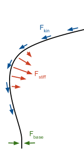
Figure 1: Conceptual illustration of forces acting on a single polymer that are not due to hydrodynamic interactions. The blue vectors indicate the buckling forces due to kinesin walkers (tangent to polymer), the red vectors show the direction and relative magnitude of stiffness forces (in the direction of $d^{4}\mathbf{r}/ds^{4}$), and the green arrows indicate a restorative force keeping the base of the polymer approximately perpendicular to the binding surface.

We now present a model for the simulation of the Sanchez et al. system. A similar method has been used successfully to simulate cytoplasmic streaming in Drosophila oocytesMonteith et al. (2016), and is based on theoretical work completed several decades ago regarding the calculation of Stokes flows created by a point force (stokeslet) near no-slip boundariesBlake (1971); Liron and Mochon (1976). A conceptual explanation of this mechanism is given below, and further details regarding theory and implementation are given in supplementary materials S-II and S-III.

An illustration of how MT bundles are simulated is given in Fig. 1. Each MT bundle is modeled as a chain of monomers (i.e. polymer) which are held an approximately fixed distance from one another by a spring force. The base of each polymer is anchored to a single point, and the polymer at the base is kept roughly perpendicular to the anchoring surface. Let the polymer be described by the curve $\mathbf{r}(s)$, where $\mathbf{r}(0)$ is the location of the polymer base, and $s$ is the arc length. We give the polymer a stiffness by implementing an energetic cost of bending proportional to curvature squared, which implies a local force at $s$ proportional to $d^{4}\mathbf{r}/ds^{4}$. Additionally, monomers feel a “buckling” force due to the drag from the walking kinesin $F_{kin}=-f_{k}d\mathbf{r}/ds$, which is parallel to the polymer and toward the polymer base. $f_{k}$ will depend linearly on the speed of the kinesin and the solvent viscosity. This force continually adds energy to the system (making it active), and has been shown to be a good representation of the average drag force due to kinesin walking along the microtubule away from the polymer base Monteith et al. (2016).

This kind of model for a single chain was first employed to understand glide assay dynamics in two dimensions Bourdieu et al. (1995). In three dimensions, periodic waves develop whose dynamics have been analyzed in detail Monteith et al. (2016), and related theoretical work has recently also been performed De Canio et al. (2017). However, scaling can be used to get the relevant length and timescales Bourdieu et al. (1995). The average radius of curvature depends on the strength of the buckling force $f_{k}$, and the elastic constant of a filament characterizing its stiffness $k_{stiff}$. The radius of curvature over quite a wide range of parameters can be shown to be $R=(k_{stiff}/(\beta f_{k}))^{1/3}$, where $\beta\approx 0.05$. Likewise, the angular frequency is $\omega=f_{k}/(\nu R)$, where $\nu$ is the hydrodynamic drag coefficient per unit length. Although there is a fairly large experimental uncertainty in parameters used to model a Drosophila oocyte, this model finds quite good agreement with the experimental time and length scales. $R$ was predicted to be $25-54\mu$m, close to the $16.3\pm 2.2\mu$m observed. Likewise, the time scale was predicted to be $203-1094$s, which is in the observed range of $370\pm 42$s. It is interesting that the length and time scales observed by Sanchez et al. are also quite close to these numbers, and that the frequency of biological cilia beating is often three orders of magnitude higher than this.

Polymers also feel hydrodynamic forces. As the force from the kinesin causes the polymers to buckle, we begin to see complex motion. Each monomer acts as a point force (stokeslet) in the surrounding fluid. This force, that a monomer exerts on the fluid, is simply the sum of all of the other forces on the monomer: because the Reynolds number is nearly zero, there are no inertial terms, meaning the force is transferred perfectly from the monomer to the fluid. As this is a Stokes flow, the flow contributions from all stokeslets add linearly, and we can (in principle) calculate the flow everywhere. However, we only need to calculate the fluid velocity at points with monomers. Therefore, the evolution can be calculated via a pairwise sum over all monomers (see the supplemental materials S-II.

We also assume all polymer motion is two dimensional with a constant value of $z$, which is physically sensible when considering the geometry of the Sanchez et al. experiments. In this experiment, MT bundles were observed between glass slides, with a height $H$, of approximately $10\mu$m, creating a narrow channel for which fluid can flow. For this reason, we adopt a two dimensional geometry. In addition, the no-slip boundaries of the plates have a large impact on the hydrodynamic forces between monomersBlake (1971); Liron and Mochon (1976), which we give explicitly in the supplemental materials S-II. Other close-range contact forces were also used (repulsion from anchoring surface, monomer-monomer repulsion), and these are explained in the supplementary materials S-III.

We can now address at the qualitative level the mechanism by which we propose the metachronal waves observed by Sanchez et al. form. As kinesin walk away from the polymer bases, the polymers will tend to buckle. If a polymer is isolated, this buckling will lead to corkscrew motion or periodic wavesMonteith et al. (2016). When placed in an array, however, nearby polymers will exert hydrodynamic forces on one another that tend to synchronize their motion. If these hydrodynamic forces are sufficiently strong, this can cause a transition from disordered motion to aligned MTs and correlated motion.

Despite the fact that this model was developed to explain and simulate cytoplasmic streaming, its mechanism can be easily adapted for related biological phenomena. Indeed, when the conditions of the Sanchez et al. experiment are simulated in the same way, we observe metachronal waves. It is not clear if this is formally a transition or a more continuous crossover effect, but the results found make strong predictions that should be testable experimentally. In the following, we present the results of these simulations and discuss the required conditions for metachronal wave formation.

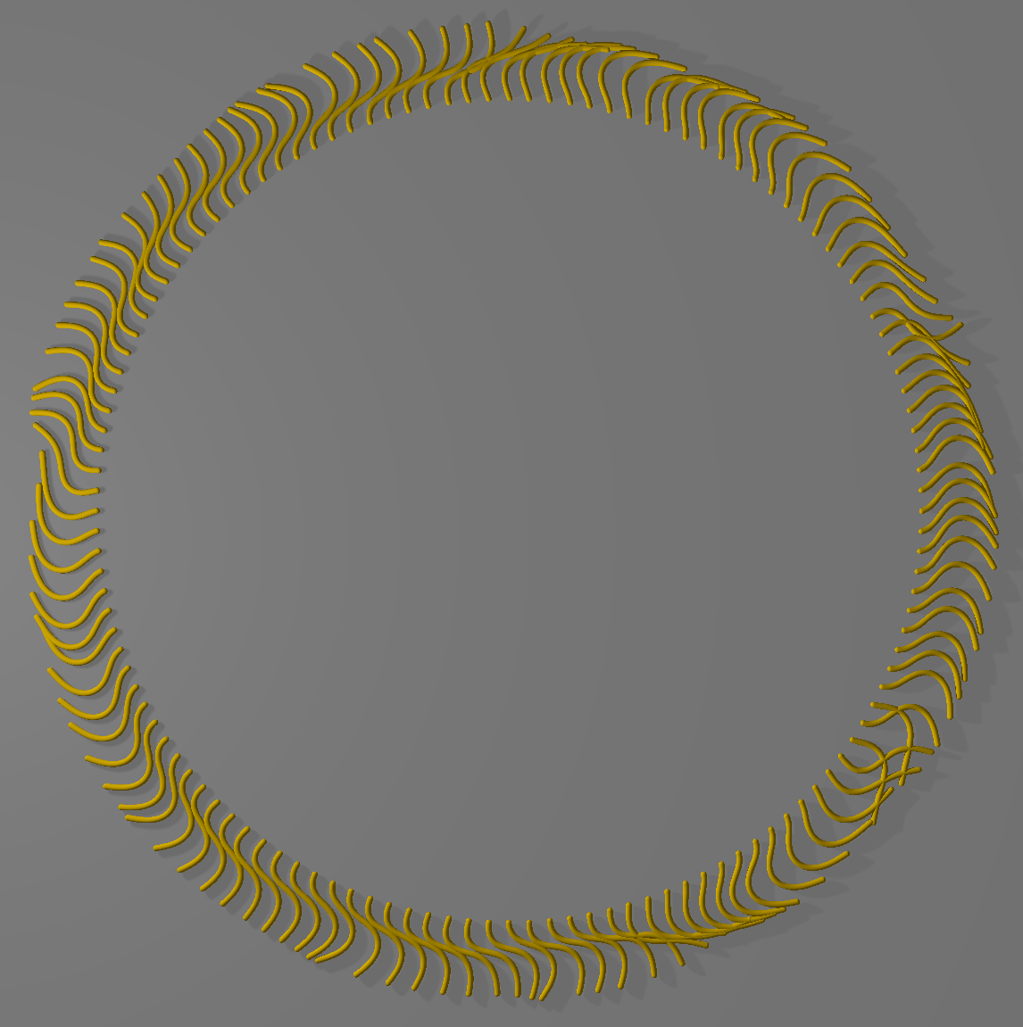
(a)

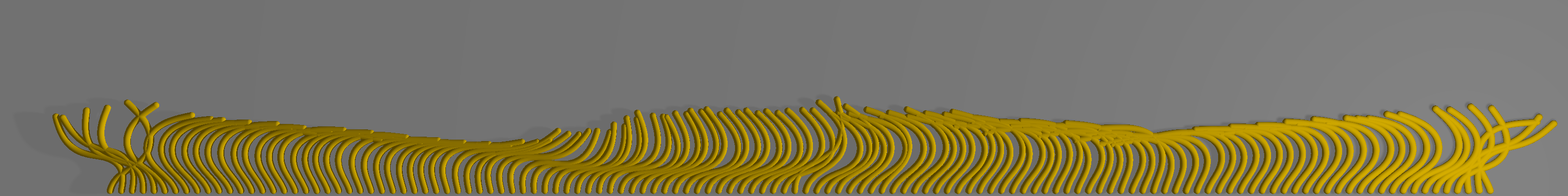
(b)

Figure 2: Simulated metachronal wave formation for 128-polymer arrays in (a) circular and (b) planar geometries. In both cases, $k_{oseen}=0.1$, $k_{stiff}=10.0$, $H=1$.

Videos of select simulations are included in the Supplementary Materials. Fig. 2 shows some still frames of simulated arrays demonstrating metachronal wave behavior in both the planar and circular geometries.

We characterize the behavior of each system using the correlation function for the chain ends $x(i,t)$,

$$C(\Delta i,\Delta t)=\langle\Delta x(i+\Delta i,t+\Delta t)\Delta x(i,t)\rangle,$$ (1)

where

$$\Delta x(i,t)=x(i,t)-\langle x(i,t)\rangle.$$

The average is performed over all chain indices $i$, and time $t$, after a period of equilibration. Figs. 3, 4, and 5 show correlation functions for planar and a circular geometries (for the circular geometry, the polar angle $\theta$ is the position variable rather than $x$). In the following, we will discuss these and examine how the system responds to changes in the strength of the interaction tensor, $k_{oseen}$, $k_{stiff}$, and height $H$. It should be noted that changes in the viscosity or kinesin velocity and density (that affect $f_{k}$), can be absorbed into a rescaling of time, and of $k_{stiff}$.

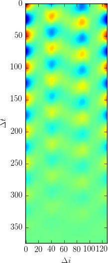
(a)

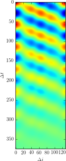
(b)

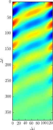
(c)

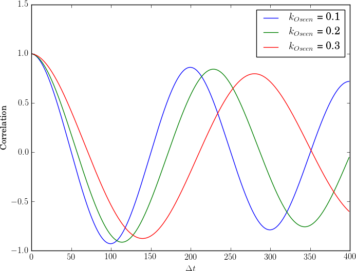
(d)

Figure 3: Full correlation functions for circular geometry with $H=1$ and $k_{stiff}=10$, with $k_{oseen}=$ 0.1, 0.2, and 0.3 (a-c, respectively). The correlation function at $\Delta i=0$ for all of these values of $k_{oseen}$ are shown in (d).

$k_{oseen}$, has a dramatic effect on the type of wave behavior seen, or whether it is observed at all. This strength is a function of the hydrodynamic effects of kinesin walking along microtubules, and will depend on their density and speed, as explained in detail in Ref. Monteith et al. (2016). Fig. 3 shows the correlation results of three 128-polymer simulations in the same circular geometry shown in Fig. 2(a) for three different values of $k_{oseen}$. There is an overall strengthening of the metachronal behavior as $k_{oseen}$ is increased from $0.1$ to $0.2$. The sign of the slope reflects the initial conditions of the system. Long lived waves travel predominantly in a single direction over long times scales resulting in a slope of the crests of the correlation function that can either be positive or negative. Similar crests are seen in the analysis of the real experimental data Sanchez et al. (2011). With this circular geometry, the correlation function must be periodic, which is why it rises again when $i$ becomes large.

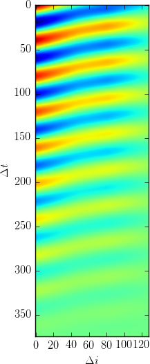
(a)

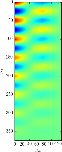
(b)

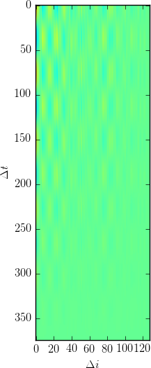
(c)

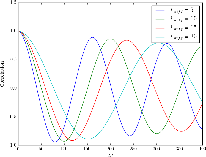
(d)

Figure 4: Full correlation functions for planar geometry with $H=1$ and $k_{oseen}=0.1$, with $k_{stiff}=$ 5.0, 10.0, and 20.0 (a-c, respectively). The correlation function at $\Delta i=0$ for all of these values of $k_{stiff}$ are shown in (d).

The polymer stiffness $k_{stiff}$ also has an interesting effect on metachronal wave formation. Fig. 4 shows the correlation functions for $k_{stiff}=$ 5.0, 10.0, and 20.0 in a planar geometry. While Figs. 4(a-b) are qualitatively similar, we do see an apparent decrease in the metachronal wavelength. Figs. 4(c-d) show that if the polymer is made too stiff, no metachronal behavior is observed at all. In general, planar geometry appears to cause more coherence in the motion of the different bundles, and the correlation function is dominated by motion at the longest lengths and time scales.

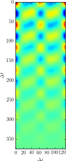
(a)

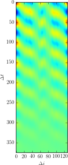
(b)

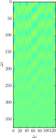
(c)

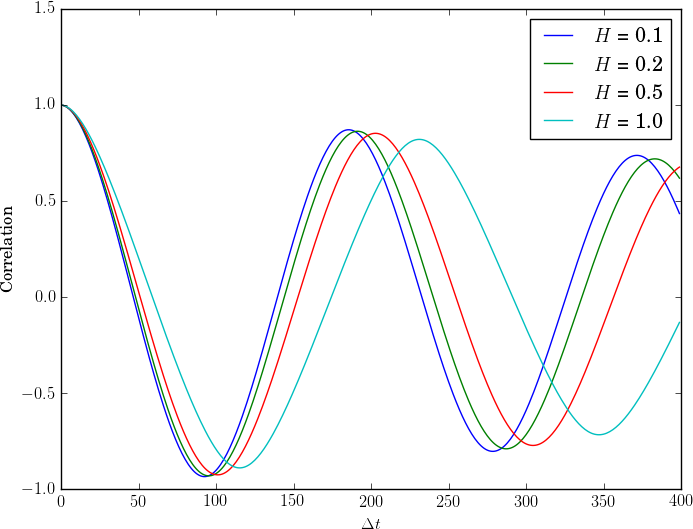
(d)

Figure 5: Full correlation functions for circular geometry with $k_{stiff}=10$, $k_{oseen}=0.2$, and $H$ = 1.0, 0.5, and 0.1 (a-c, respectively). The correlation function at $\Delta i=0$ for all of these values of $H$ are shown in (d).

The distance between plates, $H$, has a considerable effect on the dynamics as well. Longer range, more coherent motion is observed when $H$ is larger, and short range, less coherent motion when $H$ is small. See Fig. 5. This is to be expected due to the strong screening effect that these boundary conditions impose. Smaller $H$ reduces the hydrodynamic coupling, causing a decrease in coherence.

When comparing these results to those of Sanchez et al., we find that the basic features agree. The videos included in the supplemental materials qualitatively mimic the experimental videos, and the experimental correlation analysis agrees quite well with the simulations. More importantly, this agreement between theory and experiment was reached from first principles. We only use a handful of forces in our simulations, and each force has a physical justification for being used.

There are potential shortcomings of this model that may result in some differences between experiment and theory. The first is that the experiments observe bundles of microtubules that taper away from their base. The hydrodynamics are not expected to be uniform along the length of a chain. In addition these bundles will, for short enough times, behave like rigid material, but for longer times, because they are connected through walking kinesin molecules, will behave more as individual mictrotubules with a greatly reduced elastic constant. On the time scales of the motion, we expect to be in the latter regime. However the details of the hydrodynamics and elasticity in these bundles is still not understood experimentally. In fact, as we mentioned earlier, the polarity of individual MT’s is not known experimentally, and arguments for their unipolarity are given in the supplementary information, S-IV. But still, the basic mechanism of dynamic buckling due to kinesin drag, and metachronal waves being generated by hydrodynamic coupling, is robust over a wide parameter range, so we believe that these complications, aside from unipolarity, will not alter the basics of our explanation.

At a more technical level, there are other things that may make a slight difference to the results here. The bundles are constrained to move only in the $xy$-plane, and while it is true that MT motion is nearly 2-dimensional, there is some room in the $z-$direction that MT bundles can occupy. Additionally, this model does not account for the fluid boundary condition at the anchoring surface. This may introduce some errors if a monomer becomes close ($\sim H$) to the anchoring plane. However, because of the screening effects of the plates, this should not alter the behavior at distances large compared to the plate separation. We have tested for this by adding image charges to the planar case, and found that their effects on correlations are small, as expected.

In conclusion, we have developed a model for the spontaneous formation of wavelike behavior in active polymer arrays that only requires two ingredients: semi-flexible chains tethered to a surface, and motors walking from their bases to their tips. The hydrodynamics in their confined geometry gives rise to metachronal waves that appear remarkably similar to what is observed experimentally Sanchez et al. (2011); Sanchez and Dogic (2013). There is no need to posit additional mechanisms that force individual bundles to oscillate. This all happens as a consequence of Newton’s laws and fluid mechanics, allowing us to gain a better understanding of how metachronal waves form with considerable predictive power. As such, we have examined new parameter spaces and have demonstrated boundaries between different types of metachronal behavior and regimes in which no metachronal behavior exists. It would be of great interest to test these predictions experimentally. Given the simplicity and robust nature of this mechanism, and the ubiquity of microtubules and kinesin in cells, it gives one further impetus to look for other places in biology where this kind of behavior can be found.

J.M.D. thanks Bill Saxton, Itamar Kolvin, Alex Tayar, and Zvonimir Dogic for useful discussions. S.E.M. was partially supported by the ARCS Foundation. This work was also supported by the Foundational Questions Institute <http://fqxi.org>.

References

- Sanchez et al. (2011) T. Sanchez, D. Welch, D. Nicastro, and Z. Dogic, Science 333, 456 (2011).
- Sanchez and Dogic (2013) T. Sanchez and Z. Dogic, in Methods in enzymology, Vol. 524 (Elsevier, 2013) pp. 205–224.
- Afzelius (2004) B. A. Afzelius, J. Pathol. 204, 470 (2004).
- Okada et al. (2005) Y. Okada, S. Takeda, Y. Tanaka, J., C. I. Belmonte, and N. Hirokawa, Cell 121, 633 (2005).
- Brokaw (1975) C. J. Brokaw, Proceedings of the National Academy of Sciences 72, 3102 (1975).
- Camalet et al. (1999) S. Camalet, F. Jülicher, and J. Prost, Physical Review Letters 82, 1590 (1999).
- Lindemann and Lesich (2010) C. B. Lindemann and K. A. Lesich, J Cell Sci 123, 519 (2010).
- Sleigh (1969) M. A. Sleigh, Int. Rev. Cytol. 25, 31 (1969).
- Sleigh (1974) M. A. Sleigh, ed., Cilia and Flagella (Academic Press, 1974).
- Gheber and Priel (1989) L. Gheber and Z. Priel, Biophys. J. 55, 183 (1989).
- Gueron et al. (1997) S. Gueron, K. Levit-Gurevich, N. Liron, and J. J. Blum, Prot. Natl. Acad. Sci. USA 94, 6001 (1997).
- Needleman et al. (2004) D. J. Needleman, M. A. Ojeda-Lopez, U. Raviv, K. Ewert, J. B. Jones, H. P. Miller, L. Wilson, and C. R. Safinya, Physical review letters 93, 198104 (2004).
- Pazour et al. (2005) G. J. Pazour, N. Agrin, J. Leszyk, and G. B. Witman, J Cell Biol 170, 103 (2005).
- Kruse and Jülicher (2000) K. Kruse and F. Jülicher, Physical Review Letters 85, 1778 (2000).
- Liverpool and Marchetti (2003) T. B. Liverpool and M. C. Marchetti, Physical Review Letters 90, 138102 (2003).
- Lagomarsino et al. (2003) M. C. Lagomarsino, P. Jona, and B. Bassetti, Phys. Rev. E 68, 021908 (2003).
- Guirao and Joanny (2007) B. Guirao and J.-F. Joanny, Biophysical journal 92, 1900 (2007).
- Elgeti and Gompper (2013) J. Elgeti and G. Gompper, Proceedings of the National Academy of Sciences 110, 4470 (2013).
- Niedermayer et al. (2008) T. Niedermayer, B. Eckhardt, and P. Lenz, Chaos: An Interdisciplinary Journal of Nonlinear Science 18, 037128 (2008).
- Monteith et al. (2016) C. E. Monteith, M. E. Brunner, I. Djagaeva, A. M. Bielecki, J. M. Deutsch, and W. M. Saxton, Biophys. J. 110, 2053 (2016).
- Blake (1971) J. R. Blake, Mathematical Proceedings of the Cambridge Philosophical Society 70, 303 (1971).
- Liron and Mochon (1976) N. Liron and S. Mochon, Journal of Engineering Mathematics 10, 287 (1976).
- Bourdieu et al. (1995) L. Bourdieu, T. Duke, M. Elowitz, D. Winkelmann, S. Leibler, and A. Libchaber, Physical Review Letters 75, 176 (1995).
- De Canio et al. (2017) G. De Canio, E. Lauga, and R. E. Goldstein, Journal of The Royal Society Interface 14, 20170491 (2017).