A MODEL-INDEPENDENT TEST OF COSMIC ISOTROPY WITH LOW-Z PANTHEON SUPERNOVAE

Abstract

The assumption of homogeneity and isotropy on large scales is one of the main hypothesis of the standard cosmological model. In this paper, we revisit a test of cosmological isotropy using type Ia supernova (SN Ia) distances provided by the latest SN Ia compilation available, namely, the Pantheon compilation. We perform a model-independent analysis by selecting low-redshift subsamples lying in two redshift intervals, i.e., $z\leq 0.10$ and $z\leq 0.20$. By mapping the directional asymmetry of cosmological parameters across the sky, we show that the current SN Ia data favours the hypothesis of cosmic isotropy, as the anisotropy found in the maps can be mostly ascribed to the non-uniform sky coverage of the data rather than an actual cosmological signal. These results confirm that there is null evidence against the cosmological principle in the low-redshift universe.

1 Introduction

The assumption of cosmological homogeneity and isotropy, i.e., the Cosmological Principle (CP), constitutes a fundamental pillar of modern Cosmology (see, e.g., Goodman 1995; Clarkson & Maartens 2010) and implies that cosmic distances and ages can be directly derived from the Friedmann-Lemaître-Robertson-Walker (FLRW) metric. Given that any violation of the CP would have major consequences to our description of the Universe, it is of crucial importance to determine whether it actually holds true in light of observational data. If not, the current concordance model of Cosmology ($\Lambda$CDM), for instance, would need to be profoundly revised and reformulated.

One of the most direct ways to probe isotropy is through the angular dependence of the Type Ia Supernovae (SN Ia) Hubble diagram. Using this information, we can assess how the best-fit cosmological parameters vary across the sky. Any hint of large-scale departure from isotropy would be revealed if these maps disagree with synthetic data-sets based on the concordance model, or idealised sky distribution of data points. Thus far, most of analyses performed with SNe Ia data showed good agreement with the isotropy assumption (Kolatt & Lahav, 2001; Schwarz & Weinhorst, 2007; Antoniou & Perivolaropoulos, 2010; Colin et al., 2011; Cai & Tuo, 2012; Kalus et al., 2013; Cai et al., 2013; Appleby et al., 2015; Bengaly et al., 2015; Javanmardi et al., 2015; Lin et al., 2016; Bengaly, 2016; Andrade et al., 2018; Deng & Wei, 2018a, b; Sun & Wang, 2018a, b). Nevertheless, potential indications of isotropy departure were found at CMB latest data (Planck Collaboration et al., 2016; Schwarz et al., 2016), as well as in the dipole anisotropy of radio source number counts (Singal, 2011; Bengaly et al., 2018). Hence, further investigations on this subject are still needed.

In this work, we revisit the isotropy test with cosmic distances, as performed in (Bengaly et al., 2015; Bengaly, 2016), with the latest SN Ia compilation, the so-called Pantheon compilation (Scolnic et al., 2018). Some recent analyses confirmed previous results, i.e., null evidence for isotropy violation from these data (Sun & Wang, 2018b; Deng & Wei, 2018b). However, these works assumed a priori the concordance model to describe the SN Ia distances, thus testing consistency with it. We perform our analyses in a low-$z$ range instead, which allows us to do it in a model-independent way using a cosmographic approach (Visser, 2004). We found that the celestial anisotropy of cosmographic parameters is mostly due to the non-uniform distribution of SN Ia data points, and that it displays excellent concordance with Monte Carlo simulations based on the concordance model.

Figure 1: Left panel: The sky distribution of Pantheon SN Ia at $z\leq 0.10$. Right panel: The number of objects encompassed in each hemisphere selected for our analyses (see text for description).

Figure 2: Same as Figure 1, but for the SN Ia lying in the $z\leq 0.20$ interval instead.

2 Observational data and method

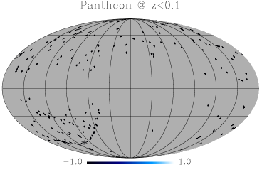
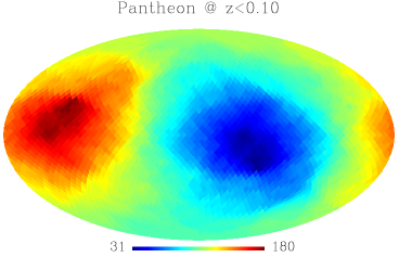
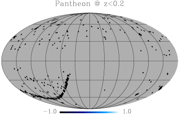
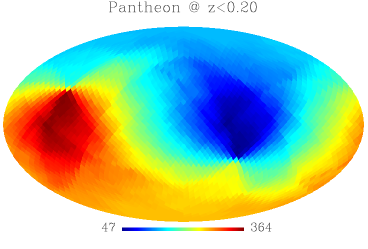
In our analysis, we adopt the Pantheon SN Ia compilation, which consists of the largest and most complete SN data-set at the present moment, i.e., 1049 objects lying in the interval $0.01<z<2.30$ compiled from the PanSTARRS1 Medium Deep Survey, SDSS, SNLS, in addition to many low-$z$ and HST data points. As we will focus on a model-independent analysis, we will only select objects at $z\leq 0.10$ and $z\leq 0.20$, thus reducing our sample to 211 and 411 data points, respectively. The sky distribution of the selected SN Ia at $z\leq 0.10$ can be visualized on the left panel of Fig. 1, whereas the left panel of Fig. 2 shows the SNe Ia at $z\leq 0.20$. On the other hand, the right panel of both figures display the asymmetry in the number of SN Ia in hemispheres whose symmetry axes coincide pixel centers defined according to HEALPix (Górski et al., 2005) $N_{\rm side}=16$ grid resolution. Then, we can note how non-uniform are the SN celestial distributions at both redshift ranges, as the number of objects varies from 31 to 180 across the sky at $z\leq 0.10$, and from 47 to 384 at $z\leq 0.20$.

Assuming that the FLRW metric holds true, one can expand the scale factor around the present time, and then measure distances regardless of the Universe dynamics. This is the well-known cosmographic approach (see, e.g. Weinberg (1972)). The luminosity distance reads

$$D_{\rm L}(z)=3000h^{-1}_{0}\left[z+(1-q_{0})(z^{2}/2)+O(z^{3})\right]\;,$$ (1)

where $z$ is the redshift observed in the comoving rest frame with respect to the expansion of the Universe, $h_{0}$ and $q_{0}$ are the dimensionless Hubble constant and decelerating parameter at present time, respectively, for $D_{\rm L}(z)$ given in Mpc. In order to avoid the issue of divergences up to higher redshifts, we parametrize the redshift variable by $y\equiv z/(1+z)$ (Cattoen & Visser, 2007). Therefore, we can rewrite the luminosity distance in terms of $y$ such as

$$D_{\rm L}(y)=3000h^{-1}_{0}\left[y+(3-q_{0})(y^{2}/2)+O(y^{3})\right]\;.$$ (2)

Therefore, the distance modulus can be written as

$$\mu(y)=5\log_{10}\left({D_{\rm L}(y)/\rm{Mpc}}\right)+25\;.$$ (3)

As shown in Eq. 2, the luminosity distance depends only on $h_{0}$ and $q_{0}$ up to the second order in redshift. Therefore, we restrict our analysis up to that order. As shown in Bengaly et al. (2015), this truncation does not bias $\mu$ in the interval $z\lesssim 0.2$.

We probe the isotropy of the Pantheon SN Ia distances by mapping the directional dependence of $h_{0}$ and $q_{0}$ and considering two redshift intervals, i.e., $z\leq 0.10$ and $z\leq 0.20$, similarly to previous analyses in the literature (Kolatt & Lahav, 2001; Schwarz & Weinhorst, 2007; Antoniou & Perivolaropoulos, 2010; Kalus et al., 2013; Bengaly et al., 2015; Javanmardi et al., 2015; Bengaly, 2016). This is done by defining hemispheres whose symmetry axes are given by HEALPix (Górski et al., 2005) pixel centers at $N_{\rm side}=16$ grid resolution, and then estimating the $h_{0}$ and $q_{0}$ best-fits for all SN Ia enclosed in such hemispheres. To do so, we minimize the following quantity

$$\chi^{2}=\sum_{i}\left[(\mu^{\rm th}(\mathbf{p},y_{\rm i})-\mu^{\rm obs}_{\rm i})^{2}/\sigma_{\rm i}\right]^{2}\;,$$ (4)

when fitting each parameter $\mathbf{p}$, being $\mathbf{p}=h_{0}$ or $q_{0}$ in our analysis. In the above equation, $i$ represents the $i$-th data point belonging to each hemisphere, $\mu^{\rm obs}_{\rm i}$ denotes its distance modulus, $\sigma^{2}_{\rm i}$ corresponds to its respective uncertainty, and $\mu^{\rm th}(\mathbf{p},y_{\rm i})$ is the theoretically expected distance modulus calculated according to Eq. (3). We only use the statistical errors for $\mu^{\rm obs}_{\rm i}$ in our analyses, as the full covariance matrix would significantly degrade the constraints at such low-$z$ ranges. Hence, we obtain $3072$ values of $h_{0}$ and $q_{0}$ across the entire sky, which will be hereafter referred to as Hubble-maps and $q$-maps, respectively.

The statistical significance of these maps is computed from two sets of 1000 Monte Carlo (MC) realizations according to the following prescriptions:

• MC-iso: The SN original positions in the sky are changed according to an isotropic distribution;

• MC-lcdm: The SN original distance moduli are changed according to a value drawn from a normal distribution $\mathcal{N}(\mu_{\rm fid},\sigma)$, i.e., a distribution centered at $\mu_{\rm fid}$, which is fixed at a fiducial Cosmology following $h_{0}=0.678$ and $q_{0}=-0.574$, and whose standard deviation is given by the original distance modulus uncertainty, $\sigma$.

We quantify the level of anisotropy in the data and the MCs by defining

$$\Delta p\equiv p^{\rm max}_{0}-p^{\rm min}_{0}$$ (5)

being $p^{\rm max}_{0}$ and $p^{\rm min}_{0}$, respectively, the maximum and minimum best fits for $p\rightarrow h_{0}$ or $q_{0}$ obtained across the entire celestial sphere.

Thus, we compare the $\Delta h$ and $\Delta q$ between the real data and these 1000 MCs by computing the fraction of realizations with $\Delta h$ or $\Delta q$ at least as great as the observed one, hence defined as our $p$-value. If we find less than $5\%$ of agreement between them, we can state that its anisotropy can be either ascribed to the non-uniform celestial distribution of SN Ia (for the MC-iso), or to a departure of the concordance model (for the MC-lcdm).

3 Results

Figure 3: The hubble-map of Pantheon SN at $z\leq 0.10$ (left panel), and the q-map at the same redshift range (right panel). We note that $h_{0}$ ranges from $0.685$ to $0.711$ in the left panel, while $q_{0}$ ranges from $-0.22$ to $1.23$ in the central one,

Figure 4: The same as Fig. (3) for the $z\leq 0.20$ SN Ia instead. We note that $h_{0}$ ranges from $0.676$ to $0.700$, $q_{0}$ ranges from $-0.85$ to $-0.18$.

Figure 5: The $\Delta h$ values of the MC-lcdm (pink histogram) and MC-iso (blue histogram) realizations compared to the actual data for $z\leq 0.1$ (left panel) and $z\leq 0.20$ (right panel), respectively. The vertical line corresponds to the real data result.

Figure 6: The same as Fig. 5 for $\Delta q$.

		hubble-map
$z$ range	$\Delta h$	MC-iso $p$-value (%)	MC-lcdm $p$-value (%)
$z\leq 0.10$	$0.026$	$0.3$	$7.3$
$z\leq 0.20$	$0.024$	$<0.1$	$7.1$
		q-map
$z$ range	$\Delta q$	MC-iso $p$-value (%)	MC-lcdm $p$-value (%)
$z\leq 0.10$	$1.440$	$37.4$	$47.9$
$z\leq 0.20$	$0.670$	$0.1$	$12.5$

Table 1: Respectively: The redshift range, $\Delta h$, as defined in Eq. (5), and the $p$-values for each MC data-set. Below are shown the same quantities for the $q$-maps.

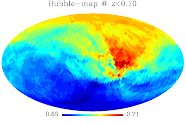
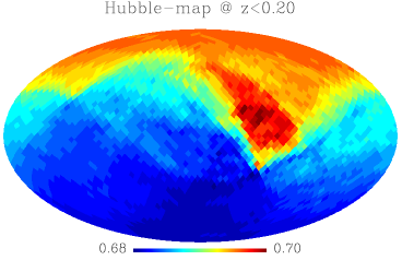
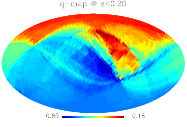
We show the hubble-maps for both $z\leq 0.10$ and $z\leq 0.20$ in the left panels of Figures 3 and 4, respectively. In the central panels of the same figures, we display the results for the $q$-maps in the same redshift intervals. As presented in Table 1, the hubble-maps are in excellent agreement with previous results, such as $\Delta h=0.030$ obtained by Kalus et al. (2013) using the Constitution compilation for $z\leq 0.20$, as well as $\Delta h=0.023$ from Union2.1 for $z\leq 0.10$, as reported by Bengaly (2016). If we allow for the $1\sigma$ error-bars in both $h^{\rm max}_{0}$ and $h^{\rm min}_{0}$ values, we then obtain $\Delta h=0.026\pm 0.086$ ($z\leq 0.10$) and $\Delta h=0.024\pm 0.058$ ($z\leq 0.20$), which is fully compatible with the $h_{0}$ uncertainty due to cosmic variance, that is, $\Delta_{h_{0}}=0.015$ according to Camarena & Marra (2018) (see also Ben-Dayan et al. 2014). Regarding the $q$-maps, we find $\Delta q=1.440$ at $z\leq 0.10$, and $\Delta q=0.670$ at $z\leq 0.20$. Allowing again for the $1\sigma$ error-bars in $q^{\rm max}_{0}$ and $q^{\rm min}_{0}$, we obtain $\Delta q=1.440\pm 0.617$ and $\Delta q=0.670\pm 0.228$, respectively, at $z\leq 0.10$ and $z\leq 0.20$ redshift ranges. We can clearly see that the highest $h_{0}$ and $q_{0}$ regions coincide with those hemispheres with the lowest SN Ia counts, as shown in Figures 1 and 2. This potentially indicates a bias in both hubble- and $q$-maps due to it.

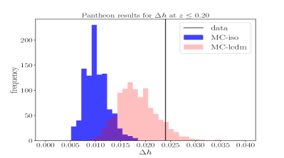
We show the results of the MC analyses in Fig. 5 for the hubble-maps in both redshift intervals, whereas Fig. 6 exhibits the results for the $q$-maps. For the hubble-maps, we can readily note that the MC-lcdm shows stronger agreement with the actual $\Delta h$ than the MC-iso realizations for both cases. This result shows that the $\Delta h$ obtained from the data is not unexpected in the $\Lambda$CDM scenario, and that its value is mostly due to the non-uniform celestial distribution of SN Ia, as suggested in the right panels of Figures 3 and 4. This is also reflected in the $p$-values shown in the third and fourth columns of Table 1, as very few isotropic MCs ($p$-value $<1$%) gave $\Delta h\geq 0.026$, yet the $p$-value increases to $\sim 7$% for the MC-lcdm case. Similar conclusions can be drawn for the q-maps, since the $p$-values significantly increase in the MC-lcdm realizations compared to the MC-iso ones, as depicted in both panels of Fig. 6, and in the last two columns of the lower part of Table 1. In fact, the agreement between the real and simulated data-sets for the q-map is stronger than the hubble-map case at all redshift ranges. These results are also compatible with previous works, such as Bengaly et al. (2015); Bengaly (2016), in which the anisotropy found in the cosmological parameters were stronger than expected from simulations assuming a perfectly uniform distribution of objects. Hence, we conclude that there is null evidence for anomalous anisotropy in cosmic distances since most of the $\Delta h$ and $\Delta q$ are due to the high asymmetry of data points in the sky, and that they fully agree with simulations that assume the concordance model given the uncertainties of the real data.

4 Final Remarks

Following previous analyses (Bengaly et al., 2015; Bengaly, 2016) we tested the cosmological isotropy using the recently released SN Ia compilation, i.e., the Pantheon data set. As in those analyses, we looked for signatures of isotropy departure by mapping the cosmographic parameters $h_{0}$ and $q_{0}$ across the sky, namely the hubble- and $q$-maps, and by estimating their statistical significance with MC simulations as well. For this purpose, we produced two sets of MCs: one that redistributes the SN in an uniform way, MC-iso, and another that assumes the cosmic distances to be given by the $\Lambda$CDM model within the error bars of the original data, MC-lcdm. We obtained $\Delta h=0.026\pm 0.086$ ($z\leq 0.10$) and $\Delta h=0.024\pm 0.058$ ($z\leq 0.20$), besides $\Delta q=1.440\pm 0.617$ and $\Delta q=0.670\pm 0.228$, also at $z\leq 0.10$ and $z\leq 0.20$, respectively. We found excellent agreement between the Pantheon results and previous analyses using older SN Ia compilations for $\Delta h$, whose value is also compatible with the cosmic variance estimative. Moreover, the MC-lcdm shows much stronger agreement with real data compared to the MC-iso for both hubble- and $q$-maps.

Finally, it is important to emphasize that the anisotropies herein reported are mostly due to non-uniform angular distribution of SN Ia, thus a selection effect, rather than a real departure of the concordance model. Therefore, the FLRW Universe can describe low-$z$ SN Ia observations very well, which guarantees the validity of the CP. In future works, different methods to test the cosmological isotropy assumption, as those presented in (Marinucci & Peccati, 2011; Jun & Genton, 2012; Hitczenko & Stein, 2012; Guinness & Fuentes, 2016; Sahoo et al., 2017), can be readily envisaged and performed in light of larger, more homogeneous cosmological data sets, that will be provided in the years to come. Among potential applications, we list the SN Ia sample from LSST (LSST Science Collaboration et al., 2009), luminosity distance measurements from standard sirens with next-generation gravitational wave experiments (Cai et al., 2018; Lin et al., 2018), besides large-area galaxy surveys such as SKA (Schwarz et al., 2015). Given all these observational data and statistical machinery available, we should be able to definitely underpin the validity of CP at large scales.

References

- LSST Science Collaboration et al. (2009) LSST Science Collaboration, Abell, P. A., Allison, J., et al. 2009, arXiv:0912.0201
- Planck Collaboration et al. (2016) Planck Collaboration, Ade, P. A. R., Aghanim, N., et al. 2016, A&A, 594, A16
- Andrade et al. (2018) Andrade, U., Bengaly, C. A. P., Alcaniz, J. S., & Santos, B. 2018, Phys. Rev. D, 97, 083518
- Antoniou & Perivolaropoulos (2010) Antoniou, I., & Perivolaropoulos, L. 2010, J. Cosmology Astropart. Phys, 12, 012
- Appleby et al. (2015) Appleby, S., Shafieloo, A., & Johnson, A. 2015, ApJ, 801, 76
- Ben-Dayan et al. (2014) Ben-Dayan, I., Durrer, R., Marozzi, G., & Schwarz, D. J. 2014, Phys. Rev. Lett., 112, 221301
- Bengaly et al. (2015) Bengaly, C. A. P., Bernui, A., & Alcaniz, J. S. 2015, ApJ, 808, 39
- Bengaly (2016) Bengaly, C. A. P., 2016, J. Cosmology Astropart. Phys, 4, 036
- Bengaly et al. (2018) Bengaly, C. A. P., Maartens, R., & Santos, M. G. 2018, J. Cosmology Astropart. Phys, 4, 031
- Cai & Tuo (2012) Cai, R.-G., & Tuo, Z.-L. 2012, J. Cosmology Astropart. Phys, 2, 004
- Cai et al. (2013) Cai, R.-G., Ma, Y.-Z., Tang, B., & Tuo, Z.-L. 2013, Phys. Rev. D, 87, 123522
- Cai et al. (2018) Cai, R.-G., Liu, T.-B., Liu, X.-W., Wang, S.-J., & Yang, T. 2018, Phys. Rev. D, 97, 103005
- Camarena & Marra (2018) Camarena, D., & Marra, V. 2018, arXiv:1805.09900
- Cattoen & Visser (2007) Cattoen, C., & Visser, M. 2007, arXiv:gr-qc/0703122
- Chang et al. (2018) Chang, Z., Lin, H.-N., Sang, Y., & Wang, S. 2018, MNRAS,
- Clarkson & Maartens (2010) Clarkson, C., & Maartens, R. 2010, Classical and Quantum Gravity, 27, 124008
- Colin et al. (2011) Colin, J., Mohayaee, R., Sarkar, S., & Shafieloo, A. 2011, MNRAS, 414, 264
- Deng & Wei (2018a) Deng, H.-K., & Wei, H. 2018, Phys. Rev. D, 97, 123515
- Deng & Wei (2018b) Deng, H.-K., & Wei, H. 2018, arXiv:1806.02773
- Gonçalves et al. (2018) Gonçalves, R. S., Carvalho, G. C., Bengaly, C. A. P., Jr., et al. 2018, MNRAS, 475, L20
- Goodman (1995) Goodman, J. 1995, Phys. Rev. D, 52, 1821
- Górski et al. (2005) Górski, K. M., Hivon, E., Banday, A. J., et al. 2005, ApJ, 622, 759
- Guinness & Fuentes (2016) Guinness, J. & Fuentes, M. 2016, Journal of Multivariate Analysis, 143, 143
- Hitczenko & Stein (2012) Hitczenko, M. & Stein, L. M. 2012, Statistical Methodology, 9, 1, 211
- Javanmardi et al. (2015) Javanmardi, B., Porciani, C., Kroupa, P., & Pflamm-Altenburg, J. 2015, ApJ, 810, 47
- Jun & Genton (2012) Jun, M. & Genton, M. G. 2012, Statistica Sinica 22, 1737
- Kalus et al. (2013) Kalus, B., Schwarz, D. J., Seikel, M., & Wiegand, A. 2013, A&A, 553, A56
- Kolatt & Lahav (2001) Kolatt, T. S., & Lahav, O. 2001, MNRAS, 323, 859
- Lin et al. (2016) Lin, H.-N., Wang, S., Chang, Z., & Li, X. 2016, MNRAS, 456, 1881
- Lin et al. (2018) Lin, H.-N., Li, J., & Li, X. 2018, European Physical Journal C, 78, 356
- Marinucci & Peccati (2011) Marinucci, D. & Peccati, G. 2011, Random Fields on the Sphere: Representation, Limit Theorems and Cosmological Applications, pp. 356. ISBN 0521175615, 9780521175616, Cambridge University Press
- Ntelis et al. (2017) Ntelis, P., Hamilton, J.-C., Le Goff, J.-M., et al. 2017, J. Cosmology Astropart. Phys, 6, 019
- Sahoo et al. (2017) Sahoo, I., Guinness, J., Reich, B. J., et al. 2017, arXiv:1711.04092
- Schwarz & Weinhorst (2007) Schwarz, D. J., & Weinhorst, B. 2007, A&A, 474, 717
- Schwarz et al. (2015) Schwarz, D. J., Bacon, D., Chen, S., et al. 2015, Advancing Astrophysics with the Square Kilometre Array (AASKA14), 32
- Schwarz et al. (2016) Schwarz, D. J., Copi, C. J., Huterer, D., & Starkman, G. D. 2016, Classical and Quantum Gravity, 33, 184001
- Scolnic et al. (2018) Scolnic, D. M., Jones, D. O., Rest, A., et al. 2018, ApJ, 859, 101
- Singal (2011) Singal, A. K. 2011, ApJ, 742, L23
- Sun & Wang (2018a) Sun, Z. Q., & Wang, F. Y. 2018, arXiv:1804.05191
- Sun & Wang (2018b) Sun, Z. Q., & Wang, F. Y. 2018, MNRAS, 478, 5153
- Visser (2004) Visser, M. 2004, Classical and Quantum Gravity, 21, 2603
- Weinberg (1972) Weinberg, S. 1972, Gravitation and Cosmology: Principles and Applications of the General Theory of Relativity, by Steven Weinberg, pp. 688. ISBN 0-471-92567-5. Wiley-VCH , July 1972., 688